Parametrization of approximate algebraic surfaces by lines

Theoretical Computer Science 315 (2004) 627–650www.elsevier.com/locate/tcs

Parametrization of approximate algebraiccurves by lines�

Sonia P(erez-D(+aza , Juana Sendrab , J. Rafael Sendraa ;∗aDepartamento de Matem�aticas, Universidad de Alcal�a, Facultad de Ciencias, Apartado de Correos 20,

E-28871 Madrid, SpainbDepartamento de Matem�aticas, Universidad Carlos III, E-28911 Madrid, Spain

Abstract

It is well known that irreducible algebraic plane curves having a singularity of maximummultiplicity are rational and can be parametrized by lines. In this paper, given a tolerance �¿ 0and an �-irreducible algebraic plane curve C of degree d having an �-singularity of multiplicityd−1, we provide an algorithm that computes a proper parametrization of a rational curve that isexactly parametrizable by lines. Furthermore, the error analysis shows that under certain initialconditions that ensures that points are projectively well de4ned, the output curve lies within theo5set region of C at distance at most 2

√2�1=(2d) exp(2).

c© 2004 Elsevier B.V. All rights reserved.

Keywords: Approximate algebraic curves; Rational parametrization; Hibrid symbolic-numeric methods

1. Introduction

Over the past several years, many authors have approached computer algebra prob-lems by means of symbolic-numeric techniques. For instance, among others, methodsfor computing greatest common divisors of approximate polynomials (see [6,9,15,29]),for determining functional decomposition (see [10]), for testing primality (see [21]),for 4nding zeros of multivariate systems (see [9,16,18]), for factoring approximatepolynomials (see [11,20,30,31]), or for numerical computation of GrCobner basis (see[28,36]) have been developed.

� Authors partially supported by BMF2002-04402-C02-01, HU2001-0002 and GAIA II (IST-2002-35512).∗ Corresponding author.E-mail addresses: [email protected] (S. P(erez-D(+az), [email protected] (J. Sendra),

[email protected] (J.R. Sendra).

0304-3975/$ - see front matter c© 2004 Elsevier B.V. All rights reserved.doi:10.1016/j.tcs.2004.01.010

mailto:[email protected]



628 S. P�erez-D�)az et al. / Theoretical Computer Science 315 (2004) 627–650

Similarly, hybrid (i.e. symbolic and numeric) methods for the algorithmic treatmentof algebraic curves and surfaces have been presented. For instance, computation ofsingularities have been treated in [3,5,13,22,26], implicitization methods have been pro-posed in [12,14], and the numerical condition of implicitly given algebraic curves andsurfaces have been analyzed (see [17]). Also, piecewise parametrizations are provided(see [11,23,19]) by means of combination of both algebraic and numerical techniquesfor solving di5erential equations and rational B-spline manipulations.

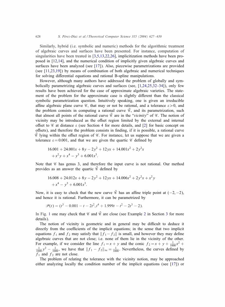
However, although many authors have addressed the problem of globally and sym-bolically parametrizing algebraic curves and surfaces (see, [1,24,25,32–34]), only fewresults have been achieved for the case of approximate algebraic varieties. The state-ment of the problem for the approximate case is slightly di5erent than the classicalsymbolic parametrization question. Intuitively speaking, one is given an irreducibleaIne algebraic plane curve C, that may or not be rational, and a tolerance �¿0, andthe problem consists in computing a rational curve JC, and its parametrization, suchthat almost all points of the rational curve JC are in the “vicinity” of C. The notion ofvicinity may be introduced as the o5set region limited by the external and internalo5set to C at distance � (see Section 4 for more details, and [2] for basic concept ono5sets), and therefore the problem consists in 4nding, if it is possible, a rational curveJC lying within the o5set region of C. For instance, let us suppose that we are given atolerance �= 0:001, and that we are given the quartic C de4ned by

16:001 + 24:001x + 8y − 2y2 + 12yx + 14:001x2 + 2y2x

+ x2y + x4 − y3 + 6:001x3:

Note that C has genus 3, and therefore the input curve is not rational. Our methodprovides as an answer the quartic JC de4ned by

16:008 + 24:012x + 8y − 2y2 + 12yx + 14:006x2 + 2y2x + x2y

+ x4 − y3 + 6:001x3:

Now, it is easy to check that the new curve JC has an aIne triple point at (−2;−2),and hence it is rational. Furthermore, it can be parametrized by

P(t) = (t3 − 0:001 − t − 2t2; t4 + 1:999t − t2 − 2t3 − 2):

In Fig. 1 one may check that C and JC are close (see Example 2 in Section 3 for moredetails).

The notion of vicinity is geometric and in general may be diIcult to deduce itdirectly from the coeIcients of the implicit equations; in the sense that two implicitequations f1 and f2 may satisfy that ‖f1 −f2‖ is small, and however they may de4nealgebraic curves that are not close; i.e. none of them lie in the vicinity of the other.For example, if we consider the line f1 = x + y and the conic f2 = x + y + 1

1000x2 +

11000y

2 − 11000 , we have that ‖f1 − f2‖∞ = 1

1000 . Nevertheless, the curves de4ned byf1 and f2 are not close.

The problem of relating the tolerance with the vicinity notion, may be approachedeither analyzing locally the condition number of the implicit equations (see [17]) or

S. P�erez-D�)az et al. / Theoretical Computer Science 315 (2004) 627–650 629

Fig. 1. Curve C (left) and curve JC (right).

studying whether for almost every point P on the original curve, there exists a pointQ on the output curve such that the Euclidean distance of P and Q is signi4cantlysmaller than the tolerance. In this paper our error analysis will be based on the secondapproach. From this fact, and using [17], one may derive upper bounds for the distanceof the o5set region.

In [4], the problem described above is studied for the case of approximate irreducibleconics, rational cubics and quadrics, and the error analysis for the conic case is pre-sented. In this paper, although we do not give an answer for the general case, we extendthe results in [4] by showing how to solve the question for the special case of curvesparametrizable by lines. More precisely, we provide an algorithm that parametrizesapproximate irreducible algebraic curves of degree d having an �-singularity of multi-plicity d−1 (see Section 2). We illustrate the results by some examples (see Section 3),and we analyze the numerical error showing that the output rational curve lies withinthe o5set region of the input perturbated curve at distance at most 2

√2�1=(2d) exp(2)

(see Section 4).

2. Numerical parametrization by lines

It is well known that irreducible algebraic curves having a singularity of maximummultiplicity are rational, and that they can be parametrized by lines. Examples of curvesparametrizable by lines are irreducible conics, irreducible cubics with a double point,irreducible quartics with a triple point, etc. In this section, we show that this property isalso true if one considers approximate irreducible algebraic curves that “almost” havea singularity of maximum multiplicity.

Before describing the method for the approximate case, and for reasons of com-pleteness, we brieQy recall here the algorithmic approach for symbolically parametrize


curves having a singularity of maximum multiplicity. The geometric idea for these typeof curves is to consider a pencil of lines passing through the singular point if the curvehas degree bigger than 2, or through a simple point if the curve is a conic. In thissituation, all but 4nitely many lines in the pencil intersect the original curve exactlyat two di5erent points: the base point of the pencil and a free point on the curve.The free intersection point depends rationally on the parameter de4ning the line, and ityields a rational parametrization of the curve. More precisely, the symbolic algorithmfor parametrizing curves by lines (where the trivial case of lines is excluded) can beoutlined as follows (see [33,34] for details):Symbolic parametrization by lines• Given an irreducible polynomial f(x; y) ∈K[x; y] (K is an algebraically closed 4eld

of characteristic zero), de4ning an irreducible aIne algebraic plane curve C ofdegree d¿1, with a (d− 1)-fold point if d¿3.

• Compute a rational parametrization P(t) = (p1(t); p2(t)) of C.1. If d= 2 take a point P on C, else determine the (d− 1)-fold point P of C.2. If P is at in4nity, consider a linear change of variables such that P is transformed

into an aIne point. Let P= (a; b).3. Compute

A(x; y; t) =

@(d−1)f@(d−1)x

1(d− 1)!

+@(d−1)f@(d−2)x@y

t(d− 2)!

+ · · · +t(d−1)

(d− 1)!@(d−1)f@(d−1)y

@df@dx

1d!

+@ df

@(d−1)x@yt

(d− 1)!+ · · · +

t d

d!@ df@dy

:

and return

P(t) = (−A(P; t) + a;−tA(P; t) + b):

Remark. The parametrization can also be obtained as

P(t) =(−gd−1(1; t)

gd(1; t)+ a;

−tgd−1(1; t)gd(1; t)

+ b);

where gd(x; y) and gd−1(x; y) are the homogeneous components of g(x; y) =f(x + a;y + b) of degree d and d − 1, respectively. Observe that both components of P(t)have the same denominator.

Now, we proceed to describe the method to parametrize by lines approximate alge-braic curves. For this purpose, we distinguish between the conic case and the generalcase. The main di5erence between these two cases is that in the case of conics, ifthe approximate curve is irreducible, the rationality is preserved. As we will see, theresults obtained for conics are similar to those presented in [4]. Afterwards, the ideasfor the 2-degree case will be generalized to any degree and therefore results in [4]will be extended. Throughout this section, we 4x a tolerance �¿0 and we will use thepolynomial ∞-norm; i.e if p(x; y) =

∑i; j∈I ai; jx

iy j ∈C[x; y] then ‖p(x; y)‖ is de4nedas max{|ai; j|=i; j∈ I}. In particular if p(x; y) is a constant coeIcient ‖p(x; y)‖ willdenote its module.


2.1. Parametrization of approximate conics

Let C be a conic de4ned by an �-irreducible (over C) polynomial f(x; y) ∈C[x; y];that is f(x; y) cannot be expressed as f(x; y) = g(x; y)h(x; y) + E(x; y) where g; h;E∈ C[x; y] and ‖E(x; y)‖¡�‖f(x; y)‖ (see for instance [11]). In particular, this impliesthat f(x; y) is irreducible and therefore C is rational. Thus, one may try to apply thesymbolic parametrization algorithm to C. In order to do that one has to compute asimple point on C. Furthermore, one may check whether the simple point can be takenover R and, if possible, compute it. This can be done either symbolically, for instanceintroducing algebraic numbers with the techniques presented in [35], or numericallyby root 4nding methods. If one works symbolically then the direct application ofthe algorithm will provide an exact answer. Let us assume that the simple point isapproximated. For this purpose, we introduce the notion of �-point.

De�nition 1. We say that JP= ( Ja; Jb) ∈C2 is an �-aIne point of an algebraic planecurve C de4ned by a polynomial f(x; y) ∈C[x; y] if it holds that

|f( JP)|‖f(x; y)‖ ¡ �;

that is, JP is a simple point on C computed under 4xed precision �‖f(x; y)‖.

Note that we required the relative error w.r.t ‖f(x; y)‖ because for any non-zerocomplex number � the polynomial �f(x; y) also de4nes C.

In this situation, let JP= ( Ja; Jb) be an �-aIne point of C, and let us consider theconic JC de4ned by the polynomial

Jf(x; y) = f(x; y) − f( JP):

Now, JP is really a point on JC. Furthermore, JC is irreducible. Indeed, if Jf factorsas Jf= Jg Jh then f= Jg Jh + f( JP) and |f( JP)|¡�‖f(x; y)‖, that is f is not �-irreducible,which is impossible. Therefore, we have constructed a rational conic, namely JC onwhich we know a simple point, namely JP. Hence, we may directly apply the symbolicalgorithm to C to get the rational parametrization

JP(t) = (−A( JP; t) + Ja;−tA( JP; t) + Jb);

where

A(x; y; t) =@f=@x + t(@f=@y)

(@2f=@2x)1=2! + t (@2f=@x@y) + (t2=2!)@2f=@2y:

2.2. Parametrization of approximate curves

In this subsection we deal with approximate curves of degree bigger than 2. In thiscase, the main diIculty is that the given approximate algebraic curve is, in general,non-rational even though it might correspond to the perturbation of a rational curve.The idea to solve the problem is to generalize the construction done for conics. For


this purpose, we observe that the output curve in the 2-degree case is the originalpolynomial minus its Taylor expansion up to order 1 at the �-point, i.e. the evaluationof the polynomial at the point. We will see that for curves of degree d having “almost”a singularity of multiplicity d−1 one may subtract to the original polynomial its Taylorexpansion up to order d− 1 at the quasi-singularity to get a rational curve close to thegiven one.

To be more precise, we 4rst introduce the notion of �-singularity.

De�nition 2. We say that JP= ( Ja; Jb) ∈C2 is an �-aIne singularity of multiplicity r ofan algebraic plane curve de4ned by a polynomial f(x; y) ∈C[x; y] if, for 06i+j6r−1,it holds that

‖(@i+jf=@ix@jy) ( JP)‖‖f(x; y)‖ ¡ �:

Note that an �-singularity of multiplicity 1 is an �-point on the curve. Similarly, onemay introduce the corresponding notion for �-singularities at in4nity. However, here wewill work only with �-aIne singularities taking into account that the user can alwaysprepare the input, by means of a suitable linear change of coordinates, in order to bein the aIne case. Alternatively, one may also use the method described in [9].

In this situation, we denote by L d� the set of all �-irreducible (over C) real algebraic

curves of degree d having an �-singularity of multiplicity d − 1, that we assume isreal. In the previous subsection we have seen how to parametrize by lines elements inL2� . In the following, we assume that d¿2 and we show that also elements in L d

�can be parametrized by lines.

In order to check whether a given curve C of degree d, de4ned by a polynomialf(x; y), belongs to L d

� , one has to check the �-irreducibility of f(x; y) as well asthe existence of an �-singularity of multiplicity d − 1. For this purpose, to analyzethe �-irreducibility, one may use any of the existing algorithms (e.g. [11,21,20,31]).The algorithm given in [11] has polynomial complexity. However, although the algo-rithm given in [21] has exponential complexity, in practice has very good performance.Furthermore, algorithms in [20,31] provide improvements to the methods describedin [21].

For checking the existence and computation of �-singularities of multiplicity d − 1one has to solve the system of algebraic equations:

@i+jf@ix@jy

(x; y) = 0; i + j = 0; : : : ; d− 2;

under 4xed precision � ·‖f(x; y)‖, by applying root 4nding techniques (see [9,22,26,27]).Nevertheless, one may accelerate the computation by reducing the number of equationsand degrees involved in the system. More precisely, for some i0; j0; i1; j1, such thati0 + j0 = i1 + j1 =d− 2, one computes the solutions of the system

@i0+j0f@i0x@j0y

(x; y) =@i1+j1f@i1x@j1y

(x; y) = 0;


Fig. 2. Real part of the curve C.

under 4xed precision �‖f(x; y)‖. Note that the two equations involved are quadratic.For this purpose, one may use well known methods (see for instance [9,22,26,27]).Once these solutions have been approximated, one may proceed as follows: if any ofthe roots obtained above, say JP, satis4es that∣∣∣∣

∣∣∣∣ @i+jf@ix@jy( JP)∣∣∣∣∣∣∣∣6 �‖f(x; y)‖; i + j = 0; : : : ; d− 3;

then JP is an �-singularity of multiplicity d−1; otherwise, C does not have �-singularitiesof multiplicity d− 1.

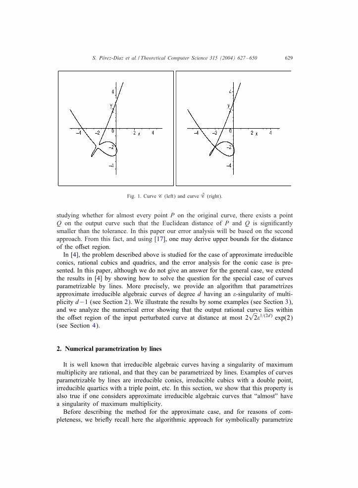
As an example (see Example 3 in Section 3), let �= 0:001, and let C be the real�-irreducible quartic de4ned by

f(x; y) = x4 + 2y4 + 1:001x3 + 3x2y − y2x − 3y3 + 0:00001y2

− 0:001x − 0:001y − 0:001:

Applying the process described above one gets that C has a 3-fold �-singularity atJP= (−0:1248595915 10−6; 0:1249844199 10−6). In Fig. 2 appears the plot of the realpart of C, and one sees that JP is “almost” a triple point of the curve.

Alternatively to the approach described above one may use the techniques presentedin [5] in combination with the Gap Theorem (see [8]), and the Test Criterion.

Now, in order to parametrize the approximate algebraic curve C∈L d� we consider

a pencil of lines Ht passing through the �-singularity JP= ( Ja; Jb) of multiplicity d− 1.That is, Ht is de4ned by the polynomial

Ht(x; y; t) = y − tx − Jb+ Jat:

If JP had been really a singularity, then the above symbolic algorithm would haveoutput the parametrization ( Jp1(t); Jp2(t)) ∈R(t)2, where Jp1(t) is the root in R(t) of


the polynomial

f(x; tx + Jb− Jat)(x − Ja)d−1

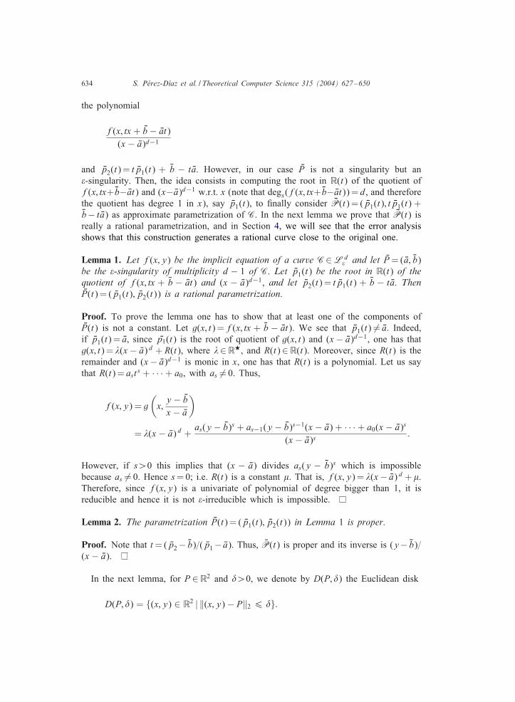
and Jp2(t) = t Jp1(t) + Jb − t Ja. However, in our case JP is not a singularity but an�-singularity. Then, the idea consists in computing the root in R(t) of the quotient off(x; tx+Jb− Jat) and (x− Ja)d−1 w.r.t. x (note that degx(f(x; tx+Jb− Jat)) =d, and thereforethe quotient has degree 1 in x), say Jp1(t), to 4nally consider JP(t) = ( Jp1(t); t Jp1(t) +Jb− t Ja) as approximate parametrization of C. In the next lemma we prove that JP(t) isreally a rational parametrization, and in Section 4, we will see that the error analysisshows that this construction generates a rational curve close to the original one.

Lemma 1. Let f(x; y) be the implicit equation of a curve C∈L d� and let JP= ( Ja; Jb)

be the �-singularity of multiplicity d − 1 of C. Let Jp1(t) be the root in R(t) of thequotient of f(x; tx + Jb − Jat) and (x − Ja)d−1, and let Jp2(t) = t Jp1(t) + Jb − t Ja. ThenJP(t) = ( Jp1(t); Jp2(t)) is a rational parametrization.

Proof. To prove the lemma one has to show that at least one of the components ofJP(t) is not a constant. Let g(x; t) =f(x; tx + Jb − Jat). We see that Jp1(t) �= Ja. Indeed,if Jp1(t) = Ja, since Jp1(t) is the root of quotient of g(x; t) and (x− Ja)d−1, one has thatg(x; t) = �(x − Ja) d + R(t), where �∈R?, and R(t) ∈R(t). Moreover, since R(t) is theremainder and (x− Ja)d−1 is monic in x, one has that R(t) is a polynomial. Let us saythat R(t) = ast s + · · · + a0, with as �= 0. Thus,

f(x; y) = g(x;y − Jbx − Ja

)

= �(x − Ja) d +as(y − Jb)s + as−1(y − Jb)s−1(x − Ja) + · · · + a0(x − Ja)s

(x − Ja)s:

However, if s¿0 this implies that (x − Ja) divides as(y − Jb)s which is impossiblebecause as �= 0. Hence s= 0; i.e. R(t) is a constant �. That is, f(x; y) = �(x− Ja) d+�.Therefore, since f(x; y) is a univariate of polynomial of degree bigger than 1, it isreducible and hence it is not �-irreducible which is impossible.

Lemma 2. The parametrization JP(t) = ( Jp1(t); Jp2(t)) in Lemma 1 is proper.

Proof. Note that t= ( Jp2 − Jb)=( Jp1 − Ja). Thus, JP(t) is proper and its inverse is (y− Jb)=(x − Ja).

In the next lemma, for P ∈R2 and �¿0, we denote by D(P; �) the Euclidean disk

D(P; �) = {(x; y) ∈ R2 | ‖(x; y) − P‖2 6 �}:


Lemma 3. Let C be an a:ne algebraic curve, de;ned by a polynomial f(x; y) ∈R[x; y], having a real �-singularity JP of multiplicity r. Then, there exists �¿0 suchthat any point Q∈D( JP; �) is also an �-singularity of multiplicity r of C.

Proof. We denote by fi; j the partial derivative @i+jf=@ix@jy. Since JP is an�-singularity of multiplicity r, for i+j= 1; : : : ; r−1, it holds that |fi; j( JP)|¡�‖f(x; y)‖.Let us denote |fi; j( JP)| = �i; j for i+j= 1; : : : ; r−1. Then, for each �i; j there exist �i; j¿0such that

�i; j = �‖f(x; y)‖ − �i;j ¡ �‖f(x; y)‖:

We consider �= min{�i; j, i + j= 1; : : : ; r − 1} (note that �¿0). On the other hand,since all partial derivatives are continuous, let M bound all partial derivatives up toorder r in the compact set D( JP; �), and let � be strictly smaller than min{�=(2M); �};note that M¿0 since otherwise it would imply that C contains a disk of points whichis impossible. Now, take Q∈D( JP; �). Then, by applying the Mean Value Theorem, wehave that for i + j= 1; : : : ; r − 1

|fi; j(Q)| 6 |fi; j( JP)| + |fi; j( JP) − fi; j(Q)| 6 �i; j + |∇(fi; j(!i; j)) · ( JP − Q)T |;

where !i; j is on the segment joining Q and JP. Then, one concludes that

|fi; j(Q)| 6 �‖f(x; y)‖ − �i; j + 2�M 6 �‖f(x; y)‖ − �+ 2�M ¡ �‖f(x; y)‖:

Therefore, Q is an �-singularity of multiplicity r of C.

Now, let C∈L d� be de4ned by the polynomial f(x; y). Then by Lemma 3, one

deduces that C has in4nitely many (d − 1)-fold �-singularities. For our purposes, weare interested in choosing the singularity appropriately. More precisely, we say thatJP= ( Ja; Jb) is a proper (d− 1)-fold �-singularity of C if the polynomial

d∑j1+j2=d−1

@j1+j2f@j1x@j2y

( JP)(x − Ja)j1 (y − Jb)j21

j1!j2!;

is irreducible over C. Note that this is always possible because a small perturbation ofthe coeIcients of a polynomial transforms it onto an irreducible polynomial.

The following theorem shows that the implicit equation of the rational curve de4nedby the parametrization generated by the above process can be obtained also, as in theconic case, by Taylor expansions at the �-singularity. In fact, the theorem includes asa particular case the result for conics. This result will avoid quotient computations andwill be used to analyze the error.

Theorem 1. Let f(x; y) be the implicit equation of a curve C∈L d� and let JP= ( Ja; Jb)

be a proper �-singularity of multiplicity d − 1 of C. Let Jp1(t) be the root in R(t)of the quotient of f(x; tx + Jb − Jat) and (x − Ja)d−1, and let Jp2(t) = t Jp1(t) + Jb − t Ja.Then the implicit equation of the rational curve JC de;ned by the parametrization


JP(t) = ( Jp1(t); Jp2(t)) is

Jf(x; y) = f(x; y) − T (x; y);

where T (x; y) is the Taylor expansion up to order d− 1 of f(x; y) at JP.

Proof. Let

f(x; y) = f( JP) +d∑

j1+j2=1

@j1+j2f@j1x@j2y

( JP)(x − Ja)j1 (y − Jb)j21

j1!j2!

be the Taylor expansion of f(x; y) at JP. Thus,

f(x; tx + Jb− t Ja) =f( JP) +d∑

j1+j2=1

@j1+j2f@j1x@j2y

( JP)(x − Ja)j1+j2 tj21

j1!j2!

= (x − Ja)d−1

(d∑

j1+j2=d−1

@j1+j2f@j1x@j2y

( JP)(x − Ja)j1+j2−d+1tj21

j1!j2!

)

+

(f( JP) +

d−2∑j1+j2=1

@j1+j2f@j1x@j2y

( JP)(x − Ja)j1+j2 tj21

j1!j2!

)

= (x − Ja)d−1M (x; t) + N (x; t);

where

N (x; t) = T (x; tx + Jb− t Ja); M (x; t) =S(x; tx + Jb− t Ja)

(x − Ja)d−1

and S(x; y) is the Taylor expansion from order d− 1 up to order d at JP. We observethat degx(M) = 1, and degx(N )6d − 2. On the other hand, let U (x; t) and V (x; t) bethe quotient and the remainder of f(x; tx+ Jb− t Ja) and (x− Ja)d−1 w.r.t. x, respectively.Then,

f(x; tx + Jb− t Ja) = (x − Ja)d−1U (x; t) + V (x; t)

with degx(V )6d− 2. Therefore,

(x − Ja)d−1(M (x; t) − U (x; t)) =V (x; t) − N (x; t):

Thus, since the degree w.r.t. x of V − N is smaller or equal d − 2, and (x − Ja)d−1

divides V − N , one gets that M =U and V =N . In this situation,

Jf( JP(t)) =f( JP(t)) − T ( JP(t)) = f( Jp1(t); t Jp1(t) + Jb− t Ja) − T ( JP(t))

= ( Jp1(t) − Ja)d−1U ( Jp1(t); t) + N ( Jp1(t); t) − T ( JP(t))

= T ( JP(t)) − T ( JP(t)) = 0:

Moreover, since JP is a proper �-singularity of multiplicity d− 1 of C, one has that Jfis irreducible, and thus JP(t) parametrizes JC.


This result can be applied to derive a similar algorithm for parametrizing approximatealgebraic curves by lines similar to the symbolic algorithm.

Numerical parametrization by lines• Given the de4ning polynomial f(x; y) of C∈L d

� , d¿2.• Compute a rational parametrization JP(t) of a rational curve JC close to C.

1. If d= 2 compute an aIne �-point JP of C, else compute a proper �-singularityJP of C of multiplicity d− 1.

2. Compute Jf(x; y) =f(x; y) − T (x; y) where T (x; y) is the Taylor expansion off(x; y) up to order d− 1 at JP.

3. Apply step 3 of the symbolic algorithm to Jf and JP.

3. Examples

In this section, we illustrate the numerical parametrization algorithm developed inSection 2 by some examples where one can check that the output rational curve JCis close to the original curve C. This behavior will be clari4ed in the error analysissection.

We give an example in detail, where we explain how the algorithm is performed,and we summarize seven other examples in di5erent tables. In these tables we showthe input curve C, the tolerance � considered, the �-singularity, the output curve JC, theoutput parametrization JP(t) de4ning the curve JC, and a 4gure representing C and JC.

Example 1. We consider �= 0:001 and the curve C of degree 6 de4ned by the poly-nomial

f(x; y) = y6 + x6 + 2:yx4 − 2:y4x + 10−3x + 10−3y + 2 · 10−3 + 10−3x4:

First of all, by applying the algorithm developed in [11], we observe that the polyno-mial f(x; y) is �-irreducible. Now, we apply the 4rst step of the Algorithm NumericalParametrization by Lines, and we compute the �-singularity. For this purpose, we de-termine the solutions of the system (see [9,27])

@4f@4x

(x; y) =@4f@4y

(x; y) = 0;

under 4xed precision �‖f(x; y)‖ = 0:002. We get four solutions

JP1 = (−0:06650062380 + 0:1157587268I; 0:06683312414 + 0:1154704132I);JP2 = (−0:06650062380 − 0:1157587268I; 0:06683312414 − 0:1154704132I);JP3 = (0:1875000000 · 10−5;−0:50000002 · 10−3);JP4 = (0:1329993725;−0:1331662483):

Only the root JP3, satis4es that∣∣∣∣∣∣∣∣ @i+jf@ix@jy

( JP3)∣∣∣∣∣∣∣∣6 0:002; i + j = 0; : : : ; 3:


Then JP= JP3 = (0:1875000000 · 10−5;−0:50000002 · 10−3) is an �-singularity of multi-plicity 5, and therefore C∈L6

0:001.Applying the second step of the Algorithm Numerical Parametrization by Lines, we

compute

Jf(x; y) = f(x; y) − T (x; y);

where T (x; y) is the Taylor expansion of f(x; y) up to order 5 at JP,T (x; y) = 0:001000000000x + 0:0010000000000y + 0:1000000173 · 10−8yx +0:1300000000 · 10−10x4 + 0:7500000034 · 10−8x3 − 0:2499999700 · 10−8y3 +0:4000000160 · 10−2xy3 + 0:1500000000 · 10−4x3y − 0:2109375027 · 10−13x2 +0:3000000000 · 10−12y4 − 0:2812500001 · 10−11y2 − 0:4218750000 · 10−10yx2 +0:3000000240 · 10−5y2x + 0:2000000000 · 10−2:One gets the curve JC de4ned byJf(x; y) = −0:1250000464 · 10−12x+ 0:1125000100 · 10−14y+ 0:9999999873 · 10−3x4 +

2:yx4−2:y4x−0:1000000173·10−8yx+y6 +x6−0:7500000036·10−8x3 +0:2499999700·10−8y3 + 0:2109375029 ·10−13x2 −0:3000000180 ·10−12y4 + 0:2812500000 ·10−11y2 −0:1500000000 · 10−4x3y − 0:4000000160 · 10−2xy3 − 0:3000000240 · 10−5y2x +0:4218750000 · 10−10yx2 + 0:1562500311 · 10−18:

Now, we apply step 3 of the symbolic algorithm to Jf and JP. Thus, we compute

A(x; y; t) =

@5 Jf@5x

15!

+@5 Jf@4x@y

t4!

+ · · · +t5

5!@5 Jf@5y

@6 Jf@6x

16!

+@6 Jf@5x@y

t5!

+ · · · +t6

6!@6 Jf@6y

=6x + 2:000000000t − 2:000000000t4 + 6yt5

1 + t6

and we return

P(t) = (−A( JP; t) + 0:1875000000 · 10−5;−tA( JP; t) − 0:50000002 · 10−3)

= ( Jp1(t); Jp2(t));

where

Jp1(t) =−2:000000000t + 0:3000000120 · 10−2t5 + 0:1875000000 · 10−5t6

1 + t6

+2:000000000t4 − 0:9375000000 · 10−5

1 + t6

and

Jp2(t) =−0:4887500200 · 10−3 − 2:000000000t4 − 0:3000000120 · 10−2t5

1 + t6

+2:000000000t − 0:5000000200 · 10−3t6

1 + t6:

See Fig. 3 to compare the input curve and the rational output curve.


Fig. 3. Input curve C (left) and output curve JC (right).

Example 2.

Input curve C16:001 + 24:001x + 8y − 2y2 + 12yx + 14:001x2

+ 2y2x + x2y + x4 − y3 + 6:001x3

Tolerance � 0:001

�-Singularity (−2; −2)

Output curve JC16:008 + 24:012x + 8y − 2y2 + 12yx

+14:006x2 + 2y2x + x2y + x4 − y3 + 6:001x3

ParametrizationJP(t) = ( Jp1(t); Jp2(t))

Jp1 = t3 − 0:001 − t − 2t2; Jp2 = t4 + 1:999t − t2 − 2t3 − 2

FiguresCurve C(left)Curve JC(right)


Example 3.

Input curve Cx4 + 2y4 + 1:001x3 + 3x2y − y2x − 3y3 + 0:00001y2

− 0:001x − 0:001y − 0:001

Tolerance � 0:001

�-Singularity (−0:1248595915 10−6; 0:1249844199 · 10−6)

Output curve JC

x4 + 2:y4 + 1:001x3 + 3:x2y − y2x − 3:y3 + 10−6y2

− 0:6243761996 · 10−13x − 0:6260915576 · 10−13y+ 0:9744187291 · 10−23 − 0:3522924910 · 10−16x2

+ 0:9991263887 · 10−6xy


Jp1 = −0:487671 · 2:0526−2:05055t2+6:15167t+0:512063·10−6t4−6:15167t3

1+2:t4 ;

Jp2 = 0:487671 · −2:05260t+2:05055t3−6:15167t2+6:15167t4+0:256287·10−6

1+2:t4 :


Example 4.

Input curve Cy5 + x5 + x4 + 0:001x + 0:001y + 0:002 + 0:001x2

+ 0:005y2 + 0:001x3

Tolerance � 0:01

�-Singularity (− 0:0002501; 0)

Output curve JCy5 + x5 + x4 + 0:6255863298·10−10x + 0:9999998183·10−3x3

+ 0:3912115701 · 10−14 + 0:3751562603 · 10−6x2

ParametrizationJP(t) = ( Jp1(t); Jp2(t)) Jp1 = − 41902244·10−6· 2384119+597t5

1+t5 ; Jp2 = −0:9987492180 t1+t5 :

FiguresCurve C (left)Curve JC (right)


Example 5.

Input curve C

−10:x + 2:y + xy4 + 862:x4y − 359:x3y2 + 3:099

− 859:967x3y + 39:x2y3 + 299:011x2y2

+ 52:x2y − 3:xy3 + 5:xy2 − 7:901xy + 687:x4

− 642:x5 − 67:989x3 + 14:x2 − 9:989y4 + y5 − 4:y3 − y2

Tolerance � 0:1

�-Singularity (0:999067678; 1:99734)

Output curve JC

10:12701492x + 1:548607302y + xy4 + 862:x4y

− 359:x3y2 − 859:9670000x3y + 39:x2y3

+ 299:0110000x2y2 + 52:18519488x2y − 3:xy3

+ 4:626307400xy2 − 7:063248589xy − 642:x5

− 67:98172465x3 + 13:33333837x2 − 9:989000000y4 + y5

− 3:999974822y3 − 0:9012712980y2 + 687:x4 + 3:247948193


Jp1 = 0:22545229 · 0:69592866·103−0:128422685·104t+0:0102:t4+4:4313t5

t5+t4+862:t+39:t3−642−359:t2

+ 0:22545229 · 0:81893515·103t2−0:19495476·103t3

t5+t4+862:t+39:t3−642−359:t2 ;

Jp2 = 0:22545229 · 0:111775629·105t−0:82845609·104t2+4:4380666t5

t5+t4+862:t+39:t3−642−359:t2

+ 0:22545229 · 0:27553162·104t3−0:35891982·103t4−0:56876434·104

t5+t4+862:t+39:t3−642−359:t2



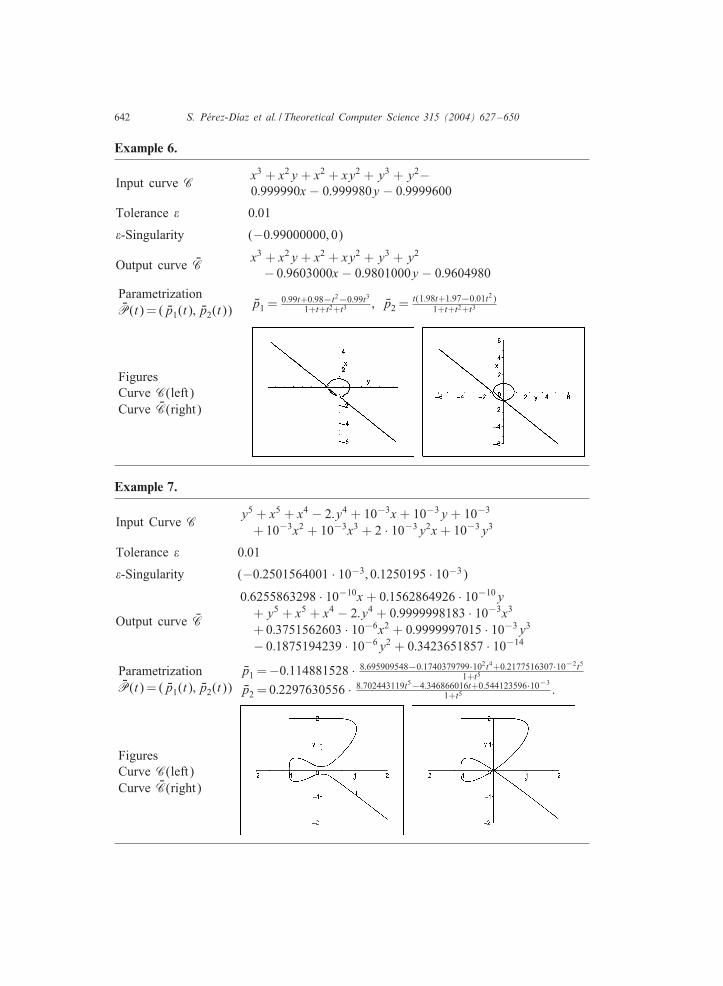
Example 6.

Input curve Cx3 + x2y + x2 + xy2 + y3 + y2−0:999990x − 0:999980y − 0:9999600

Tolerance � 0:01

�-Singularity (−0:99000000; 0)

Output curve JCx3 + x2y + x2 + xy2 + y3 + y2

− 0:9603000x − 0:9801000y − 0:9604980

ParametrizationJP(t) = ( Jp1(t); Jp2(t)) Jp1 = 0:99t+0:98−t2−0:99t3

1+t+t2+t3 ; Jp2 = t(1:98t+1:97−0:01t2)1+t+t2+t3


Example 7.

Input Curve Cy5 + x5 + x4 − 2:y4 + 10−3x + 10−3y + 10−3

+ 10−3x2 + 10−3x3 + 2 · 10−3y2x + 10−3y3

Tolerance � 0:01

�-Singularity (−0:2501564001 · 10−3; 0:1250195 · 10−3)

Output curve JC

0:6255863298 · 10−10x + 0:1562864926 · 10−10y+y5 + x5 + x4 − 2:y4 + 0:9999998183 · 10−3x3

+ 0:3751562603 · 10−6x2 + 0:9999997015 · 10−3y3

− 0:1875194239 · 10−6y2 + 0:3423651857 · 10−14


Jp1 = −0:114881528 · 8:695909548−0:1740379799·102t4+0:2177516307·10−2t5

1+t5

Jp2 = 0:2297630556 · 8:702443119t5−4:346866016t+0:544123596·10−3

1+t5 :



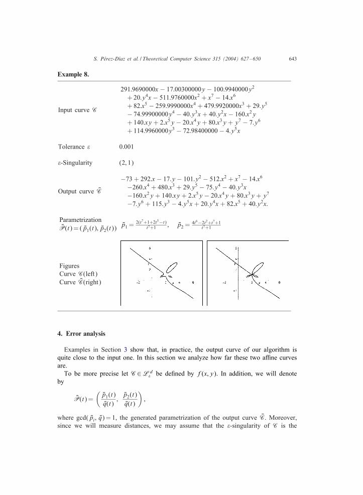
Example 8.

Input curve C

291:9690000x − 17:00300000y − 100:9940000y2

+ 20:y4x − 511:9760000x2 + x7 − 14:x6

+ 82:x5 − 259:9990000x4 + 479:9920000x3 + 29:y5

− 74:99900000y4 − 40:y3x + 40:y2x − 160:x2y+ 140:xy + 2:x5y − 20:x4y + 80:x3y + y7 − 7:y6

+ 114:9960000y3 − 72:98400000 − 4:y5x

Tolerance � 0:001

�-Singularity (2; 1)

Output curve JC

−73 + 292:x − 17:y − 101:y2 − 512:x2 + x7 − 14:x6

−260:x4 + 480:x3 + 29:y5 − 75:y4 − 40:y3x−160:x2y + 140:xy + 2:x5y − 20:x4y + 80:x3y + y7

−7:y6 + 115:y3 − 4:y5x + 20:y4x + 82:x5 + 40:y2x:

ParametrizationJP(t) = ( Jp1(t); Jp2(t)) Jp1 = 2(t7+1+2t5−t)

t7+1 ; Jp2 = 4t6−2t2+t7+1t7+1


4. Error analysis

Examples in Section 3 show that, in practice, the output curve of our algorithm isquite close to the input one. In this section we analyze how far these two aIne curvesare.

To be more precise let C∈L d� be de4ned by f(x; y). In addition, we will denote

by

JP(t) =(

Jp1(t)Jq(t)

;Jp2(t)Jq(t)

);

where gcd( Jpi; Jq) = 1, the generated parametrization of the output curve JC. Moreover,since we will measure distances, we may assume that the �-singularity of C is the


origin, otherwise one can apply a translation such that it is moved to the origin anddistances are preserved. Also we assume that ‖f(x; y)‖ = 1, otherwise we considerf(x; y)=‖f(x; y)‖. If one does not normalize the input polynomial f(x; y), a similartreatment with relative errors can be done.

In this situation, the general strategy we will follow is to show that almost any aInereal point on JC is at small distance of an aIne real point on C. For this purpose, weobserve that JP(t) is an exact parametrization of JC obtained by lines, and therefore allaIne real points on JC are obtained as the intersection of a line of the form y= tx, fort real, with JC. Then, if one intersects the curve C with the same line one gets d pointson C, counted properly, and we show that at least one of these intersection points onC is close to the initial point on JC. Also, we observe that it is enough to reason withslope parameter values of t in the interval [−1; 1] because if |t|¿1 one may apply asimilar strategy intersecting with lines of the form x= ty. Therefore, let t0 ∈R be suchthat |t0|61 and Jq(t0) �= 0. Then, the corresponding point JQ on JC is JQ= JP(t0). Let usexpressed JQ as

JQ = ( Ja; Jb) =(

Ja1

Jc;

Jb1

Jc

);

where Ja1 = Jp1(t0), Ja2 = Jp2(t0) and Jc= Jq(t0). Observe that, since we are cutting withthe line y= t0x, it holds that Jb= t0 Ja. Thus, if we write the aIne point JQ projectivelyone has that ( Ja1 : t0 Ja1 : Jc). Now, observe that if | Ja1| and | Jc| are simultaneously verysmall, i.e. very close to �, this point is not well de4ned as an element in P2(R). Forthis reason, we will assume that either | Ja1| or | Jc| is bigger than a certain bound thatdepends on the tolerance. In fact, for our error analysis, we 4x that

| Ja1|¿ �1=d or | Jc|¿ �1=d:

Furthermore, we observe that the de4ning polynomials of JC and C have the samehomogeneous form of maximum degree, and hence both curves have the same pointsat in4nity.

Now, let Q= (a; b) be any aIne point in C∩{y= t0x}; note that here it also holdsthat b= t0a. We want to compute the Euclidean distance between JQ and Q. In orderto do that, we observe that

‖ JQ − Q‖2 =√

( Ja− a)2 + ( Jb− b)2 =√

( Ja− a)2(1 + t20) 6√

2| Ja− a|:

Therefore, we focus on the problem of computing a good bound for | Ja− a|. For thispurpose we 4rst prove two di5erent lemmas that will be used as general strategies inour reasonings.

Lemma 2. It holds that

| Ja− a| 6 � · C;


where

C =

∑d−2j1+j2=0 | Ja|j1+j2 |t0|j21=j1!j2!

| Ja|d−1| Jc| :

Proof. First of all, we note that Ja is a root of the univariate polynomial Jf(x; t0x) = xd−1

( Jcx − Ja1), and that a is a root of the univariate polynomial

f(x; t0x) = xd−1( Jcx − Ja1) +d−2∑

j1+j2=0

@j1+j2f@j1x@j2y

(0; 0)xj1 (t0x)j21

j1!j2!:

Since (0; 0) is the (d− 1)-fold �-singularity of JC it holds that

‖f(x; t0x) − Jf(x; t0x)‖ = maxj1+j2=0;:::;d−2

{∣∣∣∣ @j1+j2f@j1x@j2y

(0; 0)∣∣∣∣ |t0|j2 1

j1!j2!

}

6 maxj1+j2=0;:::;d−2

{∣∣∣∣ @j1+j2f@j1x@j2y

(0; 0)∣∣∣∣}¡ �‖f(x; y)‖ = �

and thus Jf(x; t0x) can be written as

Jf(x; t0x) = f(x; t0x) + R(x) where R ∈ R[x] and ‖R(x)‖¡ �:

Therefore, by applying standard numerical techniques to measure | Ja− a| by means ofthe condition number (see for instance [7, p. 303]), one deduces that

| Ja− a| 6 � · C;where

C =

∑d−2j1+j2=0 | Ja|j1+j2 |t0|j21=j1!j2!

|@ Jf=@x( Ja; t0 Ja)| =

∑d−2j1+j2=0 | Ja|j1+j2 |t0|j21=j1!j2!

| Ja|d−1| Jc| :

Lemma 3. Let

h(x) = cn∏i=1

(x − ci) ∈ C[x] with deg(h) = n

and let �∈C be such that |h(�)|6�. Then, there exists a root ci0 of h(x) such that

|�− ci0 | 6(�|c|)1=n

:

Proof. Let us assume that for i= 1; : : : ; n, |�− ci|¿(�=|c|)1=n. Then,

|h(�)| = |c|n∏i=1

|�− ci|¿ �;

which contradicts that |h(�)|6�.


Now, we proceed to analyze | Ja−a| by using the previous lemmas. For this purpose,we distinguish di5erent cases depending on the values of | Ja1| and | Jc|:

Lemma 4. Let | Jc|¿1. Then, it holds that:1. If | Ja|¿1, then | Ja− a|6� exp(2).2. If | Ja|61, then | Ja− a|6(� exp(2))1=d.

Proof.1. If | Ja|¿1, we have that the constant C in Lemma 2 can be bounded as

C =

∑d−2j1+j2=0 | Ja|j1+j2 |t0|j2 1=j1!j2!

| Ja|d−1| Jc| =∑d−2k=0 (| Ja| + | Ja‖t0|)k =k!

| Ja|d−1| Jc|

6d−2∑k=0

(1 + |t0|)kk!| Ja|d−1−k 6

d−2∑k=0

(1 + |t0|)kk!

6 exp(1 + |t0|) 6 exp(2):

Therefore, by Lemma 2 we deduce that

| Ja− a| 6 � exp(2):

2. If | Ja|61, we have that

|f( Ja; Jat0)| =

∣∣∣∣∣ Jf( Ja; Jat0) +d−2∑

j1+j2=0

@j1+j2f@j1x@j2y

(0; 0) Jaj1 (t0 Ja)j21

j1!j2!

∣∣∣∣∣=

∣∣∣∣∣d−2∑

j1+j2=0

@j1+j2f@j1x@j2y

(0; 0) Jaj1 (t0 Ja)j21

j1!j2!

∣∣∣∣∣6

d−2∑j1+j2=0

∣∣∣∣ @j1+j2f@j1x@j2y

(0; 0)∣∣∣∣ | Ja|j1 |t0|j2 | Ja|j2 1

j1!j2!6 � exp(| Ja|(1 + |t0|))

6 � exp(2):

In this situation, by Lemma 3 we deduce that there exists a root of the univariatepolynomial f(x; t0x), that we can assume w.l.o.g. that is a, such that

| Ja− a| 6(� exp(2)

| Jc|)1=d

6 (� exp(2))1=d:

Lemma 5. Let | Jc|¡1 and | Ja1|¿1. Then, it holds that | Ja− a|6� exp(2).


Proof. Since | Jc|¡1 and | Ja1|¿1, we have that the constant C in Lemma 2 can bebounded as

C =

∑d−2j1+j2=0 | Ja|j1+j2 |t0|j21=j1!j2!

| Ja|d−1| Jc| =∑d−2k=0 (| Ja1| + | Ja1‖t0|)k | Jc|(d−2−k)=k!

| Ja1|d−1

6d−2∑k=0

(1 + |t0|)kk!| Ja1|d−1−k 6

d−2∑k=0

(1 + |t0|)kk!

6 exp(1 + |t0|) 6 exp(2):


| Ja− a| 6 � exp(2):

Finally, it only remains to analyze the case where | Jc|¡1 and | Ja1|¡1. In order todo that, we recall that we have assumed that either | Ja1| or | Jc| is bigger than �1=d. Inthe next lemma, we study these cases.

Lemma 6. It holds that:1. If | Jc|¡1 and �1=d¡| Ja1|¡1, then | Ja− a|6�1=d exp(2).2. If | Ja1|¡1 and �1=d¡| Jc|¡1, then | Ja− a|6(�1=2 exp(2))1=d.

Proof.1. If | Jc|¡1 and | Ja1|¿�1=d, we have that the constant C in Lemma 2 can be bounded

as

C =

∑d−2j1+j2=0 | Ja|j1+j2 |t0|j21=j1!j2!

| Ja|d−1| Jc| =

∑d−2j1+j2=0 | Ja1|j1+j2−d+1|t0|j21=j1!j2!

| Jc|j1+j2−d+2

=

∑d−2j1+j2=0 | Jc|d−j1−j2−2|t0|j21=j1!j2!

| Ja1|d−j1−j2−1

6

∑d−2j1+j2=0 |t0|j21=j1!j2!

| Ja1|d−1 6exp(2)| Ja1|d−1 6 exp(2) �−1+1=d


| Ja− a| 6 �1=d exp(2):

2. Let �1=d¡| Jc|¡1 and | Ja1|¡1. First we assume that | Ja1|6�1=d. Otherwise we wouldreason as in [1]. Thus, one has that | Ja1|6�1=d¡| Jc|¡1. In these conditions, we deducethat

|f( Ja; Jat0)| =

∣∣∣∣∣ Jf( Ja; Jat0) +d−2∑

j1+j2=0

@j1+j2f@j1x@j2y

(0; 0) Jaj1 (t0 Ja)j21

j1!j2!

∣∣∣∣∣=

∣∣∣∣∣d−2∑

j1+j2=0

@j1+j2f@j1x@j2y

(0; 0) Jaj1 (t0 Ja)j21

j1!j2!

∣∣∣∣∣


6d−2∑

j1+j2=0

∣∣∣∣ @j1+j2f@j1x@j2y

(0; 0)∣∣∣∣ | Ja|j1 |t0|j2 | Ja|j2 1

j1!j2!

6 � exp(| Ja|(1 + |t0|)) 6 � exp(2):

Now, by Lemma 3 we deduce that there exists a root of the univariate polynomialf(x; t0x), that we can assume w.l.o.g. that is a, such that

| Ja− a|6(� exp(2)

| Jc|)1=d

= (� · exp(2))1=d 1| Jc|1=d 6 (� exp(2))1=d 1

�1=d2

6 (� exp(2))1=d 1�1=2d

= (�1=2 exp(2))1=d:

From the previous lemmas, one deduces the following theorem.

Theorem 2. For almost all a:ne real point JQ∈ JC there exists an a:ne real pointQ∈C such that

‖ JQ − Q‖26√

2�1=2d exp(2):

Proof. Applying Lemmas 4–6 one deduces that

‖ JQ − Q‖2 =√

( Ja− a)2 + ( Jb− b)2 =√

( Ja− a)2(1 + t20)

6√

2| Ja− a| 6√

2�1=2d exp(2):

Now, let JQ= ( Ja; Jb) be a regular point on JC such that there exists Q= (a; b) ∈Cwith ‖ JQ − Q‖26

√2�1=2d exp(2) (see Theorem 2). In this situation, we consider the

tangent line to JC at JQ; i.e. T (x; y) = nx(x− Ja)+ny(y− Jb), where (nx; ny) is the unitarynormal vector to JC at JQ. Then, we bound the value ‖T (Q)‖:

‖T (Q)‖6 ‖nx‖ · |a− Ja| + ‖ny‖ · |b− Jb| 6 ‖ JQ − Q‖2(‖nx‖ + ‖ny‖)

6 2√

2�1=2d exp(2):

Therefore, reasoning as in Section 2.2 of [17] one deduces the following theorem.

Theorem 3. C is contained in the o<set region of JC at distance 2√

2�1=2d exp(2):

References

[1] S. Abhyankar, C. Bajaj, Automatic parametrization of rational curves and surfaces III: algebraic planecurves, Comput. Aided Geom. Des. 5 (1988) 321–390.

[2] E. Arrondo, J. Sendra, J.R. Sendra, Parametric generalized o5sets to hypersurfaces, J. Simbolic Comput.23 (1997) 267–285.


[3] C. Bajaj, C.M. Ho5mann, J.E. Hopcroft, R.E. Lynch, Tracing surface intersections, Comput. AidedGeom. Des. 5 (1988) 285–307.

[4] C. Bajaj, A. Royappa, Parameterization in 4nite precision, Algorithmica 27 (1) (2000) 100–114.[5] C. Bajaj, G. Xu, Piecewise approximations of real algebraic curves, J. Comput. Math. 15 (1) (1997)

55–71.[6] B. Beckermann, G. Labahn, When are two polynomials relatively prime? J. Symbolic Comput. 26

(1998) 677–689.[7] R. Bulirsch, J. Stoer, Introduction to Numerical Analysis, Springer, New York, 1993.[8] J. Canny, The complexity of robot motion planning, ACM Doctoral Dissertation Award, The MIT Press,

Cambridge, MA, 1987.[9] R.M. Corless, P.M. Gianni, B.M. Trager, S.M. Watt, The singular value decomposition for polynomial

systems, Proceedings of the ISSAC 1995, ACM Press, New York, 1995, pp. 195–207.[10] R.M. Corless, M.W. Giesbrecht, D.J. Je5rey, S.M. Watt, Approximate polynomial decomposition, in:

S.S. Dooley (Ed.), Proceedings of the ISSAC 1999, Vancouver, Canada, ACM Press, New York, 1999,pp. 213–220.

[11] R.M. Corless, M.W. Giesbrecht, I.S. Kotsireas, M. van Hoeij, S.M. Watt, Towards factoringbivariate approximate polynomials, Proceedings of the ISSAC 2001, Bernard Mourrain, London, 2001,pp. 85–92.

[12] R.M. Corless, M.W. Giesbrecht, I. Kotsireas, S.M. Watt, Numerical implicitization of parametrichypersurfaces with linear algebra. Proceedings of the Arti4cial Intelligence with Symbolic Computation(AISC 2000), Lecture Notes in Arti4cal Intelligence, Springer, Berlin, 1930, pp. 174–183.

[13] J. Demmel, D. Manocha, Algorithms for intersecting parametric and algebraic curves II: multipleintersections, Graphical Models and Image Processing: GMIP 57 (2) (1995) 81–100.

[14] T. Dokken, Approximate implicitization, in: T. Lyche, L.L. Schumakes (Eds.), Mathematical Methodsfor Curves and Surfaces in GAGD, Oslo 2000, Innovations in Applied Mathematical Series, VanderbiltUniversity Press, 2001, pp. 81–102.

[15] I.Z. Emiris, A. Galligo, H. Lombardi, Certi4ed approximate univariate GCDs, J. Pure Appl. Algebra117 and 118 (1997) 229–251.

[16] I.Z. Emiris, Pan, Y. Victor, Symbolic and numeric methods for exploiting structure in constructingresultant matrices, J. Symbolic Comput. 33(4) 2002 393–413.

[17] R.T. Farouki, V.T. Rajan, On the numerical condition of algebraic curves and surfaces. 1: Implicitequations, Comput. Aided Geom. Des. 5 (1988) 215–252.

[18] Fortune, Polynomial root-4nding using iterated eigenvalue computation, Proceedings of the ISSAC 2001,ACM Press, New York, pp. 121–128.

[19] J. Gahleitner, B. JCuttler, J. Schicho, Approximate parameterization of planar cubic curve segments,Proceedings of the Fifth International Conference on Curves and Surfaces, Saint-Malo, 2002, NashboroPress, Nashville, TN, 2002, pp. 1–13.

[20] A. Galligo, D. Rupprech, Irreducible decomposition of curves, J. Symbolic Comput. 33 (2002)661–677.

[21] A. Galligo, S.M. Watt, in: W. Kuchlin (Ed.), A Numerical Absolute Primality test for BivariatePolynomials, ISSAC 1997, Maui, USA, ACM, New York, 1997, pp. 217–224.

[22] G.H. Golub, C.F. Van Loan, Matrix Computations, The Johns Hopkins University Press, Baltimore andLondon, 1989.

[23] E. Hartmann, Numerical parameterization of curves and surfaces, Comput. Aided Geom. Des. 17 (2000)251–266.

[24] M. van Hoeij, Computing parametrizations of rational algebraic curves, in: J. von zur Gathen (Ed.),Proceedings of the ISSAC94, ACM Press, New York, pp. 187–190.

[25] M. van Hoeij, Rational parametrizations of curves using canonical divisors, J. Symbolic Comput. 23(1997) 209–227.

[26] C.M. Ho5mann, Geometric and Solid Modeling, Morgan Kaufmann Publ., Inc., Los Altos, CA, 1993.[27] S. Krishnan, D. Manocha, Solving algebraic systems using matrix computations, Sigsam Bull. ACM.

30 (4) (1996) 4–21.[28] H.M. MColler, GrCobner bases and numerical analysis, in: B. Buchberger, F. Winkler (Eds.), GrCobner

Bases and Applications, Lecture Notes in Statistics, Vol. 251, Springer, Berlin, 1998, pp. 159–178.


[29] V.Y. Pan, Numerical computation of a polynomial GCD and extensions, Tech. report, N. 2969,Sophia-Antipolis, France, 1996.

[30] V.Y. Pan, Univariate polynomials: nearly optimal algorithms for factorization and root4nding, ISSAC2001, London, Ont., Canada, ACM Press, New York, NY, USA, 2001, pp. 253–267.

[31] T. Sasaki, Approximate multivariate polynomial factorization based on zero-sum relations, Proceedingsof the ISSAC 2001, ACM Press, New York, NY, USA, 2001, pp. 284–291.

[32] J. Schicho, Rational parametrization of surfaces, J. Symbolic Comput. 26 (1998) 1–9.[33] J.R. Sendra, F. Winkler, Symbolic parametrization of curves, J. Symbolic Comput. 12 (1991) 607–631.[34] J.R. Sendra, F. Winkler, Parametrization of algebraic curves over optimal 4eld extension, J. Symbolic

Comput. 23 (1997) 191–207.[35] J.R. Sendra, F. Winkler, Algorithms for rational real algebraic curves, Fund. Inform. 39 (1999)

211–228.[36] H. Stetter, Stabilization of polynomial systems solving with Groebner bases, Proceedings of ISSAC 97,

1997, pp. 117–124.

Parametrization of approximate algebraic surfaces by lines

Documents

Transcript of Parametrization of approximate algebraic surfaces by lines