Approximate Methods for Analyzing Queueing Network ...

Approximate Methods for Analyzing Queueing Network Models of Computing Systems

K. MANI CHANDY CHARLES H. SAUER

Computer Sciences Department, Unwers~ty of Texas at Austin, Austtn, Texas 78712

The two primary issues in choosing a computing system model are credibility of the model and cost of developing and solving the model Credibility is determined by 1) the experience and biases of the persons using the model, 2) the extent to which the model represents system features, and 3) the accuracy of the solution technique. Queuemg network models are widely used because they have proven effective and are inexpensive to solve. However, most queuemg network models make strong assumptions to assure an exact numerical solution. When such assumptions severely affect credibility, slmulatmn or other approaches are used, in spite of their relatively high cost. It is the contention of this paper tha t queueing network models with credible assumptions can be solved approximately to provide credible performance estimates at low cost This contention is supported by examples of approximate solutions of queueing network models. Two major approaches to approximate solution, aggregation (decompositmn) and diffusion, are discussed

Keywords and Phrases: performance evaluatmn, queuemg networks, approximate solutions, hierarchical modeling

CR Categories" 3.81, 3.89, 4.32, 4 6, 6.20, 8 1

INTRODUCTION

Computer systems analysts use models to gain insight into the behavior of systems and to aid in systems design. The analyst has several tools (programs) at his disposal to aid in estimating the performance of systems. These include queueing models, random-number or trace-driven simulations, and statistical models. The specific tool that an analyst uses depends upon the amount of error he can tolerate, the speed with which he wishes to get results, and perhaps most importantly, the amount of faith he has in the tool. In our experience computer center managers and systems analysts generally rank tools in increasing order of credibility in the following sequence: queueing models, discrete-event random

number simulations, trace-driven simulations, monitoring systems running syn- thetic jobs, and measurements of a real workload on a real system. Unfortunately, the above ranking is generally also a ranking of tools in increasing order of cost {i.e., time used by the analyst and time used by the solution technique).

We will frame our discussion of our approximations in the context of analysts choosing between competing predictive tools, focusing attention on the three crite- ria of: 1) time used by the solution technique (speed), 2) credibility, and 3) degree of accuracy required for the problem at hand. Credibility is a subjective criterion; it varies from analyst to analyst. Yet it is crucial to the understanding of how tools are used. In particular, it is fundamental to

Permission to copy without fee all or part of this material is granted provided that the copies are not made or distributed for direct commercial advantage, the ACM copyright notice and the title of the puhhcahon and its date appear, and notme is gwen that copymg is by permission of the Association for Computing Machinery. To copy otherwise, or to republish, requires a fee and/or specific permission © 1978 ACM 0010-4892/78/0900-0281 $00 75

Computing Surveys, Vol. 10, No. 3, September 1978

282 K. M. Chandy and C. H. Sauer

CONTENTS

INTRODUCTION ! TRACTABLE QUEUEING NETWORK MODELS 2 EXAMPLES OF SYSTEMS THAT ARE ANALYZED

VIA APPROXIMATION Dmtnbutiotm and Dtsclp|mes Multiple Resource Holding Blocking Schedulers Parallehsrs. Forks and Joins Routing Summary

3 AGGREGATION (DECOMPOSITION) APPROXIMATIONS Flow-Eqmvalent Methods Passive Queue Flow-Eqmvalents Flow-Equivalents with Non-Exponentml Distributions General Closed Networks (Multiple Chains) Flow-Equivalents m Simulation Justdicatlon of Aggregation Summary

4 IMPROVEMENTS OF FLOW-EQUIVALENCE An Overwew of the Approaches Iteration Methods General Closed Queuemg Networks A Case Study for VM/370 Using Iteratlve Methods An Iteratwe Scheme for Open Network Models of Packet-

Switching Systems Product Form Methods Summary

5. FLOW-EQUIVALENT SYSTEMS AND THE MANAGEMENT OF MODELING PROJECTS

6 DIFFUSION APPROXIMATION Why Bother with Diffusion Processes ~ Mapping Between Queuemg and Dtffusmn Processes Networks Other Applications of the Dtffnslon Approxtrnatlon

an Example 7, CONCLUSION

Core Ideas A Comparmon of Analysis Techmques The Authors' Bumes APPENDIX An Example of a Complex Flow-Equivalent

Queue REFERENCES

A

the basic issue of this paper: How can approximation methods be commonly used by systems analysts in the field?

In keeping with most of the queueing network literature, we adopt the stochastic approach to approximation methods. All the systems considered in this paper are assumed to attain equilibrium; furthermore, we restrict attention (with a few ex- ceptions) to predicting the performance of systems at equilibrium. In our experience systems analysts rarely use tools to predict transient behavior; however, this situation may change as tools become increasingly flexible.

By analyzing a model we mean running a computer program that estimates queue- length distributions for one or more queues in the model. Device utilizations, mean response times, and throughputs may be de- rived from the queue length distribution. We usually ignore the problem of computing response time distributions. The problems of estimating response time distributions and their moments other than the mean are very difficult. The successful solutions have been limited to systems consisting of a single queue or a very restricted network of queues.

We generally ignore the software aspects of queueing network modeling, even though software is of critical importance. Rarely will an analyst implement a special purpose program for a specific model. Rather, the analyst will rely on existing software, perhaps adding modifications or a #pecialized user interface. Reiser and Sauer discuss queueing network software with emphasis on solution techniques [REIs78]. Sauer and MacNair survey significant queueing software with a comprehensive view of the requirements specifically associated with queueing software [SAUE78]. In this paper we only discuss software of special signifi- cance.

We put queueing network models into three categories:

1) Tractable: those which can be analyzed to give exact (as opposed to approximate) solutions in an "adequately" short time. ("Adequately" is a subjective term that will be defined later in this section.) It should be em-

Computing Surveys, Vo|. 10, No. 3, September 1978

Approximate Methods 283

phasized that tractable models often do not represent reality faithfully; the analyst should not be lulled into false security by the exactness of the solution.

2) Intolerably slow: those which can be analyzed to get exact results but which cannot be analyzed in an adequately short time.

3) Unsolved: those for which there is no known method of analysis guaranteed to give exact results.

The vast majority of queueing network models used for estimating and predicting computer system performance are of the tractable category. Rather than attempting to use a queueing network model of the second or third categories, most analysts would resort to simulation. However, constructing a simulation model with a conventional language may require a large amount of effort, and running a simulation may be computationally expensive. Thus there is a significant cost gap between queueing models and simulation models in the credibility sequence described above.

There have been three major approaches to bridging this gap:

1) Using approximate solution techniques;

2) Using a simple, tractable model to obtain bounds for performance measures of a more complex model; and

3) Using simulation tools specifically designed for solution of complex queueing models.

The following example will help to clarify these terms and approaches. Consider a model of a CDC 6000 series machine; this model consists of a central server with a queue for Peripheral Processors (PPs) ahead of the disk queues (Figure 1). To carry out an I/O operation, a job needs both a peripheral processor and a disk. When a job completes a CPU service it joins the PP queue. Only after securing a PP does the job enter one of the disk queues. The PP is held while the job is waiting in the disk queue and while the job is being serviced by the disk. After completion of disk service the job relinquishes its PP; the relinquished PP is immediately assigned to a job in the PP queue, or, if the

~o ooo, . / ' I

FIGURE 1. Central server model with peripheral processors.

PP queue is empty, the relinquished PP joins the pool of available PPs.

Consider a system with five disks, four PPs, and a level of multiprogramming of five. Assume that the PP and disk queues have a first come first served (FCFS) queueing discipline and that the CPU has a processor sharing (PS) discipline. (PS is defined as the limiting case of a no overhead round-robin discipline as the quantum goes to zero. It is used in queueing models because it is much more mathematically tractable than round-robin.) Assume the CPU service time distribution is hyperexponential and that the I/O service time distributions are exponential. (Service time distributions have a key impact on the tractability of queueing models. In Section 1 we will discuss distribution representations for those readers unfamiliar with this subject.)

This model can be represented as a Mar- kov process and an exact numerical solution can be obtained [KELL76]. (Markov processes are essential to the stochastic approach to queueing networks. This is especially true of exact solutions and specialized simulation techniques and less true of the aspects of approximation we discuss here. Section I gives a brief introduction to Mar- kov processes.) However, the time required to obtain this solution on a CDC 6600 is in the order of several minutes. We must conclude that this model falls into the category of intolerably slow models because most analysts would prefer to use alternative methods or models. If the service time distributions were arbitrary, and thus less tractable than hyperexponential and exponential forms, then this model would fall into the category of unsolved models.

Approximate solution methods can be applied to the 4 PP model [KELL76]. There is no assurance, besides empirical results, that an approximation will give satisfactory

Coraputmg Surveys, VoL 10, No. 3, September 1978


answers, but an approximation may give values very close to the exact values in less than a second of processor time. Thus the approximate solution is very attractive. Ap- proximations usually use heuristic solution techniques. The philosophy is very similar to that of artificial intelligence search strato egies: The methods are reasonable but, in general, it cannot be rigorously proven that the methods provide the desired solutions.

Consider this model with five rather than four PPs. Since the degree of multiprogramming is equal to the number of PPs, a job will never wait for a PP. Hence we can remove PPs from the model. The resulting model can be analyzed in less than a second on a CDC 6600, since the model satisfies product form (Section 1). This model falls into the tractable category.

It is possible to approximate the 4 PP system by a 5 PP tractable model because we know from experience that the 5 PP model provides a tight upper bound to the throughput of the 4 PP system. This is an instance of a complex model being analyzed by obtaining bounds for performance measures from a simpler model [SEvc77a]. Such an approach is extremely useful. How- ever, we do not consider such approaches in this paper because a general theory un- derlying such approaches is yet to be developed; cases have to be treated individ- ually. A general theory in this area would be a breakthrough in systems modeling. One must proceed cautiously; for instance, it is tempting to hypothesize that systems with more regular arrival processes (i.e., processes with smaller coefficients of variation of interarrival times, where the coefficient of variation is the standard deviation divided by the mean) may be analyzed to obtain lower bounds on the mean wait times of systems with more variable arrival processes, but this hypothesis is invalid [WOLF77].

Queueing network tools such as QSIM [FosT74] and RESQ [REIS78, SAtTE77c] allow the user to easily specify and simulate complex queueing models of the intolerably slow and unsolved categories. (RESQ also provides numerical solutions for most models of the tractable category.) A simulation of the 4 PP model above would re-

quire considerably less than a minute to obtain satisfactory results. Thus simulation would be a more reasonable method than exact numerical solution of that model.

Thus one can conclude that both approximation and simulation are viable approaches to solving this model. Though the approximation has a definite computational advantage, one must consider factors such as credibility and availability of software. For other models we may not have a choice; only one technique is viable. Our object here is to survey approximation methods for intolerably slow and unsolved models. There is no known rule for choosing between simulation and approximation methods, nor is there one for choosing among approximations. However, we feel it is important to bring approximations to the attention of a larger audience.

Before proceeding with approximations we should say a little about simulation. Simulations could be considered an approximation technique, since simulations do not provide exact results, but this is an unusual view. To clarify this point, consider a simulation of a queueing network that has a tractable numerical solution. The numerical solution is exact--if a mean response time is estimated, then that value is correct for the queueing network (though not necessarily correct for the modeled computer system). A simulation estimate of mean response time will, hopefully, be near the correct value but will usually not be equal to the correct value. Two of the principal problems with simulation are: determining how close simulation estimates are to the correct values (for the model, not the modeled system), and determining how long to run the simulation in order to obtain estimates near the correct values. These problems are still difficult for arbitrary sim- nlations, but much progress has been made toward their solution for simulations of queueing networks.

A general approach to the first problem is the estimation of confidence intervals. If a simulation run produces an estimate R for mean response time, then we produce a confidence interval estimate [R - ~, R + $] and say that the correct mean response time is in this interval with a certain


level of confidence, e.g., 90%. Suppose we run the same simulation model many times with different random number streams for each run, and estimate confidence intervals for mean response time on each run. Infor- mally, we could expect the fraction of runs with confidence interval including the correct value, to be equal to the level of confidence. Note that we are not saying that 90% (or whatever the level of confidence) of the response times are in the interval; this is a common misinterpretation of the confidence interval.

Though estimation of confidence intervals is difficult for arbitrary simulations, much progress has been made in rigorous estimation of confidence intervals for stochastic systems in equilibrium, e.g., queueing networks. The most rigorous approach is the regenerative method. Laven- berg and Slutz give an excellent introduction to this method [LAVE75], Iglehart gives a thorough survey of it [IGLE78], and Sauer and MacNair illustrate application of the method to general queueing networks [SAUE77C]. The regenerative method is not always practical; Kobayashi [KOBA78] and Sauer [SAUE77a] discuss alternative methods for queueing models.

The second problem can be handled by sequential stopping rules applied in con- junction with confidence interval estimation [LAVE77]. In brief, a sequential stopping rule allows the simulation to run for a while (a "sampling period") and then ex- amines the confidence intervals. If the intervals are "sufficiently narrow" then the simulation stops. Otherwise, additional sampling periods are run, with confidence intervals estimated after each period, until the intervals are sufficiently narrow. APLOMB, the simulation component of RESQ, provides several confidence interval methods and a sequential stopping rule.

The remainder of the paper discusses approximations. Section 1 informally describes the tractable category of models. Section 2 give examples of system models that are not in the tractable category but have been solved by approximations. Sec- tion 3 describes approximations based on aggregation of submodel results. Section 4 considers techniques for improving the ac-


curacy of aggregation approximations. Sec- tion 5 briefly discusses use of aggregation in the management of modeling projects. Section 6 describes diffusion approximations. Section 7 is an overview of approximation techniques.

1. TRACTABLE QUEUEING NETWORK MODELS

Before giving a characterization of tractable models we informally review the concepts of arrival processes, service time distributions, and Markov processes. A more thorough introduction is given by Drake [DRAK67].

Mathematicians have tried to make the representation of queueing systems as simple as possible for the sake of tractability. They then studied more complex queueing systems because they are more represent- ative of actual systems, and because they are more mathematically interesting. To keep our discussion simple we will avoid unnecessary mathematics and therefore sacrifice some rigor and general applicabil- ity.

First consider the arrival of jobs at a queue, a queue not connected to other queues. The simplest representation of the arrivals assumes that the arrivals are strictly independent of each other. To be more precise, we define a Poisson process for the arrivals: 1) observations of the arrivals during non-overlapping intervals of time are mutually independent; and 2) if we look at small enough intervals of time there will be at most one arrival per interval, and the probability of an arrival during the interval is equal to the overall rate of arrival times the length of the interval. The advantage of the Poisson representation of arrivals is that it is memoryless because of the first part of the definition; the probability of an arrival during a sufficiently small interval of time is totally independent of arrivals or lack of arrivals in the preced- ing intervals. The Poisson process is often a realistic representation of actual arrival processes but is usually chosen for queueing models because of the resulting tractability. Corresponding to the process of arrivals during a time interval, there is a distribu-



tion of times between arrivals. For the Pois- son process the corresponding interarrival time distribution is the exponential distribution; "Poisson arrivals'and "independent identically distributed exponential arrivals" are equivalent. The exponential distribution also has a memoryless property; the probability distribution for the time until the next arrival is independent of the time elapsed since the last arrival. Statements about arrivals and interarrival times can be applied to service completions and inter- departure times, respectively.

Now consider a single isolated queue with FCFS discipline. It is not reasonable to describe the queue as a whole as memoryless; even if the arrival and service processes are memoryless, the response time a job experiences will be dependent on the number of other jobs ahead of it. A Markov process has a limited amount of memory. This memory consists of distinct disjoint states. The time the process spends in a state is exponential; the memory consists only of the state distinctions. (We are con- sidering continuous time processes only, as is usually the case. Analogous statements can be made if time is represented as discrete units.)

For the queue we have just described, the Markov states are uniquely determined by the number of jobs at the queue. The queue changes from one state to another when a job arrives or departs. To obtain a solution for this process means to solve for the equilibrium probabilities of each state. This is done by solving a set of linear equations (balance equations) equating the rate at which the process leaves each state to the rate at which it enters the state. (A distinction is sometimes made between global and local balance equations. The equations just described are the global balance equations. Local balance equations ignore some of the terms of the global balance equations without affecting the solution. This is only possible for special kinds of Markov processes.)

Before returning to queueing networks, let us consider generalization of service time distributions. The same approach may be used with interarrival time distributions, but this is not often done with queueing

networks. In addition to the memoryless property, the exponential distribution also has the characteristic that the standard deviation is equal to the mean. If we want to represent a distribution with standard deviation greater than the mean but still retain as little memory as possible, we can use the hyperexponential form of Figure 2. An individual service time will be exponentially distributed with mean S~ with probability pl and exponentially distributed with mean $2 with probabilityp2. The figure represents a special case of the hyperexponential distribution; it will have coefficient of variation greater than one if pl ~ p2. S is the mean service time.

On the other hand, if we want to represent a distribution with coefficient of variation less than one, we can use the hypoexponential form of Figure 3. In this case a service time consists of the sum of several exponential service times. Both the hyperexponential and hypoexponential forms are special cases of the method of (exponential) stages [Cox55]. The method of stages allows us to closely represent most service time distributions with the only memory introduced being the distribution stage of a service time in progress. For example, if we substitute a hyperexponential service time in our single queue example, then we distin- guish Markov states of the process by the distribution stage of the job in service as well as by the number of jobs at the queue. For a discussion of equivalence of various forms of the method of stages, problems with low coefficient of variation, and a heu-

$1 : S..//(2p I)

S 2 = S//(2 p2 )

FIGURE 2. Hyperexponential form.

5d " S/D i- / 7 d '~ '

! !

u.._ .]

FIGURE 3. Hypoexponential form.


ristic solution to those problems see [SAUE75a]. For most of the remainder of the paper we assume time distributions represented by the method of stages.

Having discussed the necessary back- ground, we now characterize tractable queueing networks. A queueing network will have a tractable solution if one or more of the following conditions are met:

1) State Space Size: The balance equations can be mechanically generated and numerically solved in an adequately short amount of time.

2) State Transition Structure: The state transitions are such that recursive techniques may be used to obtain the probabilities of a few states, and then the queue length distributions can be expressed in terms of these states [Herz75, SAUE75a].

3) Product Form: The equilibrium state probability distribution consists of factors representing the states of the individual queues, i.e., P(S~ . . . . . S~) ffi (l/G) P(S~) . . . P (SK) where P(S,) is the probability that the ith queue is in state S, and P(S1 . . . . . SK) is the probability that the network is in state ( $1, . . . ,SK). ( G is a normalizing constant chosen so that the probabilities sum to one.)

Though in all three cases we can obtain performance measures such as throughput from the state probabilities, this is usually computationally inappropriate. For example, throughput can be obtained directly from normalizing constants without explicit consideration of state probabilities [DENN78a]. (See pp. 225-261, this issue.) With each of these conditions one can as- sociate programs written to solve networks meeting that condition.

The best known program corresponding to the first condition is RQA [WALL66]. Experience with this program indicates that it is useful with models having not more than a few thousand states. Unfortu- nately, many models will have much larger, perhaps infinite, state spaces. Though there have been recent results on generating balance equations [GAVE76] and on numerical methods for this problem [STEW78], there is no indication that significantly larger


state spaces will be accommodated. Note that the generality of the technique is limited only by algorithm complexity and machine resources.

The method of [HERZ75] corresponding to the second condition has only been applied to cyclic queue models (Figure 4) consisting of two queues with a fixed population of jobs. This technique is attractive because exact answers may be obtained rapidly for a variety of interesting queueing disciplines [SAUE75a]. A drawback is that a different procedure is required for each combination of queueing disciplines in the recursive method (as opposed to RQA). On the whole, this method is beneficial and is the basis of some of the approximations in Section 3. It has also been used directly in the parametric analysis of multiprocessing systems [SAuE77b].

The most important tractable models are those corresponding to the third condition, i.e., those having a product form solution. The exponential networks of [GORD67 and JACK63] have such a solution. Recent efforts [BASK75, CHAN72, DENN78, REIS75] have shown that many other networks have a product form solution. Programs such as ASQ [KELL73] and RESQ [REIs78] can analyze large product form networks in an adequately short time. In the remainder of this section we describe an important subset of the networks with product form solutions. The reader should be aware that this description is incomplete and should refer to the cited original works for formal and complete descriptions.

A queueing network of this subset consists of a set of jobs, a set of queues, an infinite source of jobs, a sink, and a set of routing rules. The jobs are partitioned into groups called "routing chains," or simply, "chains," by the routing rules. All jobs of a

CPU I/O

FIGURE 4. Cyclic queue model.



given chain are identical in their behavior. A chain is open if it is connected to the source and sink, and closed if it is not connected to these. (Thus a closed chain has a fixed population of jobs.) A network is mixed if it has both kinds of chains. The arrival process of jobs from the source is Poisson.

A queue consists of a set of devices, a queueing discipline, and a set of "local" classes. Two alternate, functionally equivalent representations of job classes have appeared in the literature. One considers classes to be global in the sense that a job belongs to that class unless it explicitly changes class. The other approach, the one we adopt, consists of classes local to queues and explicitly partitioned by routing chains. This representation facilitates implementation of solution packages [REIS78] and is often more convenient for model formulation. Global classes must also be partitioned into chains for non-simulation solutions; this is often ignored.

We will use Figure 5 to illustrate the concept of chains, local classes, and global

I class ~ II0 Device 2 I

FICuRE 5. Single routing chain with fodr classes.

Terminals c l a s s ~

classes. This figure shows three queues and four local classes. The four classes form a single routing chain because a job of one class will eventually join any other class. If we represented this network using global classes, we would need two global classes. For example, let global class A consist of local classes 1 and 2 and let global class B consist of local classes 3 and 4. When a job leaves device 1 it changes from (global) class A to class B; a job leaving device 2 changes from class B to class A.

If a job of a certain chain is to be routed to a given queue, then that queue must have one or more classes associated with the chain. The different classes of a queue may have distinct routing and, under conditions described below, may have distinct service time distributions. However, different priorities may not be assigned to the classes if a network is to retain a product form solution.

Consider the example of Figures 6, 7, and 8. They represent a computer system serving a set of terminals and also supporting a

Source Sink

Disk Queue

FIGURE 7 Open chain (batch load).

Disk Oueue

/_,, fcl ass 2 '~ ~ss.~2 ~/ Drum Oueue \

. . . . 2

FICURE 6. Closed chain (terminal load).


01sk Queue

1 2 f x 6 I i

FIGURE 8. Central server model with terminal and batch loads.

batch workload. There are two routing chains: a closed chain representing the interactive load and consisting of classes 1 through 4, and an open chain representing the batch load and consisting of classes 5, 6, and 7. Assume the closed chain population is equal to the number of terminals. As this example illustrates, we consider the routing to be from class to class rather than from queue to queue. Where alternate rout- ings are possible we must specify the relative frequency associated with each path.

For a certain class of queueing disciplines, which we shall call product form disciplines [CHAN77], different classes of a queue may have different service time distributions. The two most common in- stances of product form disciplines are 1) processor sharing, and 2) when the number of jobs at the device never exceeds the number of devices (the "infinite server" queue). The service time distributions at queues with product form disciplines may be non-exponential.

If a queue has a FCFS queueing discipline (and fewer devices than the possible queue length) then all classes of the queue must have the same exponential service time distribution. The service times may be "load (queue length) dependent.

2. EXAMPLES OF SYSTEMS THAT ARE ANALYZED VIA APPROXIMATION

We have attempted to motivate the reader to consider the use of approximations (In- troduction) and we have outlined the class of models that can be analyzed without resorting to approximations. Models that require the use of approximation techniques usually represent reality more faithfully than models that do not. The question

Approximate Methods • 289

is--which is preferable: approximate solutions to relatively faithful models, or exact solutions to relatively unfaithful (tractable) models? The question cannot be answered without empirical evidence. However, if a model ignores the existence of a resource, that model cannot be used to design or schedule the ignored resource. For example, if peripheral processors are ignored in a central server model, we cannot use that model to determine the effect of the number of PPs on performance, and then approximations, simulation, or measurement are the only alternatives.

In this section we discuss problems that force the use of approximations, because tractable models fail to represent key aspects of these problems. Our goal in this section is to introduce the reader to a wide variety of such problems and to the literature describing successful approximate solutions to these problems.

Distributions and Disciplines

If service time distributions in a model have high coefficients of variation, and if the corresponding queueing disciplines are not product form disciplines (for example, FCFS), then the values of performance measures obtained from the model may be substantially different from values obtained assuming product form [SAUE75a]. For example, consider a cyclic queue model (Fig- ure 4) with a single CPU, a single I/O device, and three jobs. If the mean CPU service is 40 ms., the coefficient of variation of CPU service time 5, and the mean I/O service time 40 ms. with an exponential distribution, then the CPU utilization with FCFS queueing at the CPU will be 64.9%. If we assume a product form CPU queueing discipline, e.g., PS, then the utilization will be 75.0%--a relative error of 15.6%.

Priority queueing disciplines usually give significantly different results than FCFS and PS. Networks of queues with priority disciplines have been solved approximately [CHAN75b, REIS76, SAUE75b, SEVC77a].

Multiple Resource Holding

A job may hold more than one resource at a time as in the peripheral processor ex-

Computing Surveys, Voi. 10, No 3, September 1978

290 • K. M. Chandy and C. H. Sauer

ample. In the example in the Introduction, a PP does not have a service time associated with it; the length of time that a PP is held depends upon other devices such as disks. Main memory is another example of an important resource that does not have a service time associated with it, though jobs need main memory to use other devices such as the CPU. Resources that do not have service times associated with them, but limit the population of jobs that may utilize other devices, are called passive resources [FoST74]. Busses and switches in multiprocessing architectures are examples of critical resources that are passive. Models with passive resources have been analyzed approximately [BRow77, BRow75, D~,NN76, KELL76, SEKI71].

Blocking

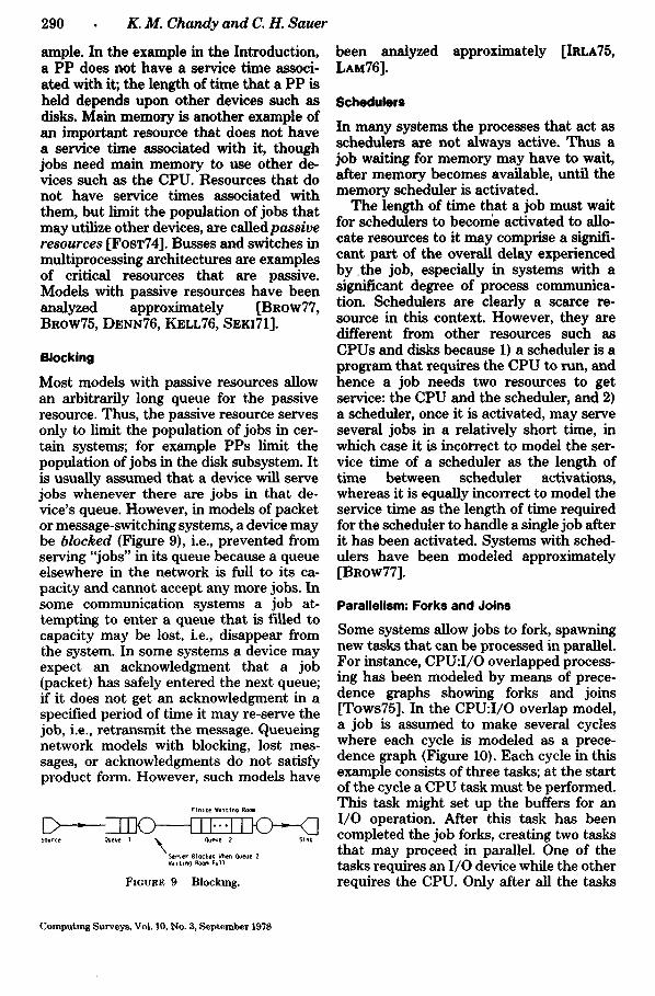
Most models with passive resources allow an arbitrarily long queue for the passive resource. Thus, the passive resource serves only to limit the population of jobs in certain systems; for example PPs limit the population of jobs in the disk subsystem. It is usually assumed that a device will serve jobs whenever there are jobs in that device's queue. However, in models of packet or message-switching systems, a device may be blocked (Figure 9), i.e., prevented from serving "jobs" in its queue because a queue elsewhere in the network is full to its capacity and cannot accept any more jobs. In some communication systems a job attempting to enter a queue that is filled to capacity may be lost, i.e., disappear from the system. In some systems a device may expect an acknowledgment that a job (packet) has safely entered the next queue; if it does not get an acknowledgment in a specified period of time it may re-serve the job, i.e., retransmit the message. Queueing network models with blocking, lost mes- sages, or acknowledgments do not satisfy product form. However, such models have

Finite t~altin 9 Roo~

D - iJJ...li -C} Source Queue 1 ~ Queue 2 Sink

\ Server 8locked When Queue 2 ~elttn9 RO0~ Full

FIGURE 9 Blocking.

been analyzed approximately [IRLA75, LAM76].

Schedulers

In many systems the processes that act as schedulers are not always active. Thus a job waiting for memory may have to wait, after memory becomes available, until the memory scheduler is activated.

The length of time that a job must wait for schedulers to become activated to allocate resources to it may comprise a significant part of the overall delay experienced by ,the job, especially in systems with a significant degree of process communication. Schedulers are clearly a scarce resource in this context. However, they are different from other resources such as CPUs and disks because 1) a scheduler is a program that requires the CPU to run, and hence a job needs two resources to get service: the CPU and the scheduler, and 2) a scheduler, once it is activated, may serve several jobs in a relatively short time, in which case it is incorrect to model the service time of a scheduler as the length of time between scheduler activations, whereas it is equally incorrect to model the service time as the length of time required for the scheduler to handle a single job after it has been activated. Systems with schedulers have been modeled approximately [BROW77].

Parallelism: Forks and Joins

Some systems allow jobs to fork, spawning new tasks that can be processed in parallel. For instance, CPU:I/O overlapped process- ing has been modeled by means of precedence graphs showing forks and joins [Tows75]. In the CPU:I/O overlap model, a job is assumed to make several cycles where each cycle is modeled as a precedence graph (Figure 10). Each cycle in this example consists of three tasks; at the start of the cycle a CPU task must be performed. This task might set up the buffers for an I/O operation. After this task has been completed the job forks, creating two tasks that may proceed in parallel. One of the tasks requires an I/O device while the other requires the CPU. Only after all the tasks


I/0 Task

FIGURE 10. model.

. s t a r t of cycle

CPU Task

~ CPU Task

? doin

Precedence graph for CPU. I /O oveNap

in a cycle have been completed can the next cycle be initiated. This model does not satisfy product form. Relatively complex overlap models have been solved by approximation methods [Tows75]. Similar problems appear in communication networks [SAuE77C].

Routing

Most queueing network models assume that the frequency at which a job will join class j after leaving class i is a constant qu, independent of the state of the system. However, there are systems in which the route that a job takes through a network of queues is designed to depend upon the state of the system. For instance, a job requiring the use of a computing system in a multi- computer network may be allowed to use any one of a pool of computers. In this case a reasonable scheduling policy is to direct the job towards that computer with the least expected delay; thus the job's path depends upon the relative congestion at different computers. Such load balancing models do not generally satisfy product form.

However, Towsley has defined a class of load balancing strategies for closed networks that do satisfy product form [Tows75]. Foschini has studied load balancing (also called dynamic routing) by means of diffusion approximations [Fosc77]. A general approach to approxi-

A p p r o x i m a t e M e t h o d s • 291

mation methods for dynamic job routing is yet to be devised.

Summary

The above problems are some of the characteristics that preclude tractable solutions. They are discussed in roughly descending order of importance, based on the amount of attention each has received in the computing literature. We do not believe a strict ordering can be given; importance of these characteristics varies from system to system. For example, it is generally assumed that CPU:I/O overlap is not significant, but individual systems may have a high degree of overlap, sufficient to make overlap more important than distributions, disciplines, or multiple resource holding.

3. AGGREGATION (DECOMPOSITION) APPROXIMATIONS

Perhaps the most important approximation strategy in queueing networks is that of aggrega t ion: one solves portions of the model in isolation ("offline") and gathers the results together ("online") to produce a solution of the whole model. This approach has also been referred to as decom- pos i t i on . One can view the strategy alter- nately as decomposition of the whole model or as aggregation of portions of the model. The choice of terminology is primarily a matter of emphasis and personal taste. Sim- ilar methods have been used for a long time in combinatorics, systems theory, and artificial intelligence. Indeed, the motivation for such methods in queueing networks came from similar approaches in general systems theory and in electrical networks.

These methods can be shown to give exact solutions for queueing networks with product form solutions [CHAN75a]. Though aggregation is computationally advanta- geous in parametric analysis of product form networks [CHAN75a], our interest will be in networks without tractable solutions. In these cases the strategy wi l l cause s o m e error because the aggregation process does not totally capture the interaction between the individual portions. The bulk of this section will be concerned with the representation of interfaces between portions.



There is another very important justification for the aggregation strategy [COUR75, COUR77]: loose coupling of subnetworks. This is in addition to the justification based on results for product form networks. We will discuss the loosely coupled justification later in this section.

Flow-Equivalent Methods

A basic approach is to replace a subnetwork of queues by a single ("composite") queue which is flow-equivalent to the subnetwork, i.e., the job flow through the composite queue is equal to the job flow through the subnetwork. This can be done repeatedly, replacing subnetworks (including those with composite queues) by flow-equivalents until the solution of the resulting network is tractable. There may be additional con- straints on the aggregation process, e.g., if we need to find performances measures for a particular queue, this queue should appear explicitly in the network after aggregation.

Determination of the flow-equivalent is not obvious. In this section we will discuss exact flow-equivalents and approximations based on variations on exact flow-equivalents proposed for other networks. In Sec- tion 4 we discuss methods for estimating the amount of error introduced and taking appropriate corrective action.

We assume, for the time being, that the subnetwork has a single routing chain and that there is a single input path to the subnetwork and a single output path from the subnetwork. We primarily discuss closed networks since most of the research and application of fiow-equivalent methods has concerned closed networks. (It should be pointed out that flow-equivalents also apply to open and mixed networks.)

First we must determine the mean service time for the composite queue. One obvious estimate would be the expected time spent in service in the subnetwork. However, this estimate may be much too low if all jobs in the composite queue receive parallel service; if only one composite queue job receives service the estimate is high if several jobs may be in service simultaneously in the subnetwork. Thus we must let the composite queue service times

be load dependent (dependent on the queue length of the composite queue).

A method for determining composite queue service times that gives exact results for product form networks [CHAN75a] is the following: Consider the subnetwork with the output fed back to the input, i.e., consider the subnetwork offline. Determine the throughput, X(n), along this feedback path for each possible job population size n in the subnetwork. Set S(n), the mean service time of the composite queue given n jobs in the queue, to 1/X(n). In other words, if the network satisfies product form, then the online behavior of the subnetwork is identical to its offline behavior.

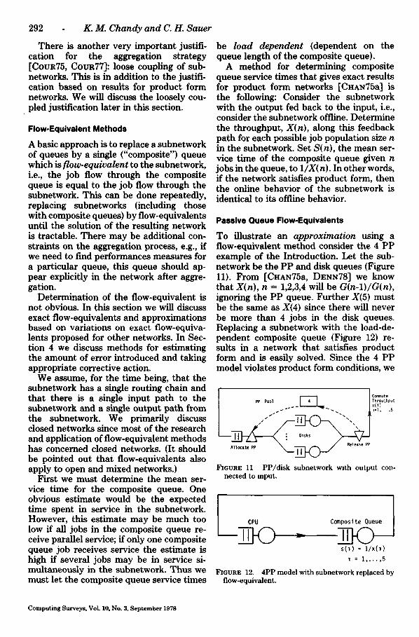
Passive Queue Flow-Equivalents

To illustrate an approximation using a flow-equivalent method consider the 4 PP example of the Introduction. Let the subnetwork be the PP and disk queues (Figure 11). From [CHAN75a, DENI~78] we know that X(n), n = 1,2,3,4 will be G(n-1)/G(n), ignoring the PP queue. Further X(5) must be the same as X(4) since there will never be more than 4 jobs in the disk queues. Replacing a subnetwork with the load-dependent composite queue (Figure 12) results in a network that satisfies product form and is easily solved. Since the 4 PP model violates product form conditions, we

~11ocate PP ~ ~ Release PP

FIGURE 11 PP/disk subnetwork with output connected to input.

CPU Composite Queue

s(1) = l/x(1) I = I , . . . ,5

FIGURE 12. 4PP model with subnetwork replaced by flow-equivalent.



f Hem°rY P°°l I I " I % I I

[ ' :

t 1 t '

~ Allocate CPU Allocate ~ ~ Release Release ~ - J Hemory pp ,,m ~ pp Hemory

Tenni nal s

FIOURE 13 PP models with memory and terminals.

cannot expect performance measures of the network of Figure 12 to be the same as the corresponding measures of the original network. But the difference is very small [KELL76], and the aggregation is both reasonable and economical.

As a numerical example, consider a PP model with parameters chosen for ease of solution and exposition. Let there be a degree of multiprogramming of 3, 2 PPs, and 2 disks. Let the mean service time at the CPU and each disk be exponential with mean 40 ms. Assume all queueing disciplines are FCFS. The routing frequencies to each disk are equal. {Remember that this network does not satisfy product form.)

The exact value for CPU utilization is 82.6% [KELL76]. If we consider the PP-disk subnetwork offiine with the output fed back to the input, we find X(1), the completion rate with 1 job in the offline system, to be 25 jobs per second. X(2) is 33.3 jobs per second and X(3) is also 33.3 since at most 2 jobs can be in the disk queues. (Without this restriction X(3) would be 37.5.) Substi- tuting this offline behavior in the CPU- composite queue network we give the composite queue a mean service time of 40 ms. with load (queue length) 1 and 30 ms. with load 2 or 3. Solving this two queue (product form) network for CPU utilization we get a value of 83.0%. Thus the error in this case is small. If we solve a similar model with 3 PPs to get an upper bound on CPU utilization, this bound would be 84.6%.

Note that this replacement of subnetworks by flow-equivalents may be repeated.

9[

Allocate /~mory CPU PP/DlSkS Releise ffemory

FIGURE 14 Network to be replaced with flow-eqmvalent

Consider the model of Figure 13. Here the 4 PP model is embedded in a network also representing memory contention and terminal think times. After making the above aggregation of the PP and disk queues, we can construct a flow-equivalent of the memory, CPU, and composite PP/disk queue in a similar manner (Figure 14). We are assuming that each job has the same fixed memory requirement. The more realistic case in which jobs require variable amounts of memory has been treated using flow- equivalents [BRow77].

Flow-Equivalents with Non-Exponential Distributions

As mentioned earlier, another situation where approximations succeed is the case of FCFS queues with non-exponential distributions. The 4 PP model had processor sharing as the CPU queueing discipline, but now suppose it was FCFS. Since the CPU service time distribution was given as hyperexponential, the model corresponding to Figure 12 would not be solvable by product form methods. However, the recursive method of [HERz75] (the second condition in Section 1) is well suited to this new two



queue model, and again we get results close to the correct solution with little computational effort [KELL76].

Let us now consider a traditional central server model (without peripheral processors) in which all service times may be non- exponential and all queueing disciplines are FCFS. Again a reasonable approach is to isolate the I /O queues and try to find a flow-equivalent composite queue representation. Pictorially this would correspond to Figures 1, 11, and 12 without the passive queues. As we explain below, the solution of the I /O subnetwork and the composite queue representation are more difficult issues than with the 4 PP network that was similar to a product form network. Though this problem has received considerable attention, the known approaches must be considered heuristic, since they are supported primarily by intuition and empirical studies rather than rigorous proofs.

Presumably we still want to use a load- dependent queue as an approximate flow- equivalent of the I /O subnetwork because it represents reality more realistically. Three key issues must be faced:

1) How do we estimate the mean service times S(n) for the (approximately) flow-equivalent system? This seems to be the most crucial issue. There are several ways of estimating the throughputs in the subnetwork; unfortunately, the better the estimation, the more expensive the method.

2) How do we choose the service time distributions in the flow-equivalent system? The emphasis in this work has been on selecting variances [SAUE75b, SEvc77b], though there has been an increasing realization that percentiles are very important [Bux77, LAZO77].

3) How do we select the queueing discipline in the flow equivalent system?

Issue 1: Selecting mean service times S(n) for the flow-equivalent system. (All of the following methods extend to general networks.)

Method 1: Figure 15 shows the network obtained by feeding the output of the I /O system back on itself. This corresponds to

taking the I /O system "offiine." If any one of the I /Os has non-exponential service times, it does not satisfy the conditions of product form, and therefore the system may be very time-consuming to analyze. However, the most accurate solution is to model this subnetwork as a discrete-state Markov process and to then determine steady-state probabilities numerically, and thus compute the exact mean service times of the flow-equivalent.

Method 2: [ZAHO77] If there are many I /Os then the number of states in the Mar- kov model of the subnetwork may be so large as to make the problem intractable. Suppose we have a technique to determine, relatively rapidly, the steady state probabilities for a network with J I/O devices. We may determine the approximate flow- equivalent composite I /O in several steps.

S tep 1: We may group together the first J I /O devices and represent this group by a flow-equivalent system with exact rather than approximate service rates. We may then group together the next J devices and determine the flow-equivalent system for this group and so on. We may choose to have exponential or non-exponential service times for the flow-equivalent system.

S tep 2: If the flow-equivalent systems in the first step are given non-exponential service times, in the second step we may determine the flow-equivalent for a group of J flow-equivalent systems obtained in the first step; thus in the second step we determine the approximate flow-equivalent for j2 devices, and we proceed in this fashion until we have an approximate flow- equivalent for the entire I /O system. This process takes logjM steps, where M is the number of I/Os.

If the flow-equivalents obtained in the first step are given exponential service

I1[ FmvnE 15 I / O subnetwork.


times,, in the second step we have a network of systems each of which satisfies product form conditions, and hence we may determine the approximate flow-equivalent for the entire' I /O system in two steps. This method will usually be less accurate than the previous method.

Method 3: We may make the assumption that all I /O devices have exponential service times, in which case the subnetwork has product form, allowing us to compute the subnetwork throughputs and the mean service rates in the approximate flow-equivalent directly. This method is very quick but probably not very accurate.

I s sue 2: Selecting service time distributions for the flow-equivalent system.

The emphasis has been on selecting the most appropriate second moment. There has been no work on the potentially valua- ble method of using percentiles of the individual service distributions to determine the percentiles of the service distribution of the composite system.

The simplest solution is to assume that the service times of the composite system are exponential (as in Method 3 above). However, this solution can result in considerable error. A more realistic solution is to estimate the second moment of the composite system from the second moments of its component parts.

Let C V be the coefficient of variation of the service time, and let a -- CV2-1. Thus a is negative for hypoexponentials, positive for hyperexponentials, and zero for exponentials. Use the subscript C for the composite system and the subscript i for the ith I /O device. Let p, be the routing frequency for a job entering the I/O system going to the ith I /O device. Sauer and Chandy propose the following heuristic formula for the coefficient of variation of the composite system [SAUE75b]:

e v e ffi Z p, CV,.

Sevcik, et al. propose a more accurate formula [SEvc77b]:

ac ffi Z P, 2a,

for heavy load conditions and also the following complex, but more accurate, equation:

A p p r o x i m a t e M e t h o d s 295

2

where M, is the mean service time of the ith I /O device and Mc the mean time a job is in service in the subnetwork.

The general problem of estimating second moments of job inter-arrival times at different points in general networks has received considerable attention, though the focus has been on networks with a single chain of jobs, one job class per queue, and FCFS queueing disciplines. Considerable work remains to be done in the area of networks with priority and other multi- class disciplines. Sevcik, et al. [SEvc77b] has the most comprehensive treatment of this issue, based in part, on earlier work [DISN74, GELE76, KOBA74, REIS74].

A summary of the results in [SEvc77b] is presented in Figures 16, 17, and 18. Once

Branch

Total ~ ~ ~ R o u t i n g Frequency P

a(Branch) = p.a(TOTAL)

FIGURE 16. Estimating second moment ofspilt flow.

Departure

Arrival v [ , , ~

/ Service

a(Departure) = Ut111zation 2 • a(Service) + ( l -Ut i l izat ion 2) • a(Arrival)

FIGURE 17 Estimatmg second moment of interde- parture times.

Branch ~ / a(t~rge)

Merqed Flow

B r a n c h 2 ~ ~ i ~ ' p - Pl = (Branch I Flow)/(Merqed Flow)

a(Merqe) = Z Pl 2 a(Branch l) FIGURE 18. Estima~ng second moment of merged

flow

Computing Surveys, Vol 10, No. 3, Sepzember 1978


the coefficient of variation is computed, the conventional approach is to represent the service time as a sequence of exponential stages (see Section 1).

Issue 3: Queueing disciplines. The queueing discipline of the composite

system does affect performance measures in the CPU-composite I/O network. Unfor- tunately, there has been very little work in the area of selecting queueing disciplines. Queueing disciplines have been selected more to reduce computational complexity than to better model the composite system. If there are many chains in the network, the assumption of processor sharing at each queue results in the simplest state-transition diagram. Usually, PS gives the same results for non-exponential distributions as exponentials, thus discarding efforts to characterize distribution form. Processor sharing allows a job to enter the I /O subsystem after another job B, but to leave before B leaves. For this reason we might choose a FCFS discipline for the flow- equivalent system for a sequence of FCFS queues in series. However, it must be emphasized that such arguments are merely educated guesses, and much empirical work needs to be done in this area.

In summary, the specification of flow- equivalent systems is still an art. However, empirical simulation work and case studies of real systems are leading to a better understanding of this problem.

General Closed Networks (Multiple Chains)

So far we have been assuming a single routing chain. The approximation techniques can be extended to multiple chains, but relatively little has been done in this area. The ease or difficulty of the extension depends on the similarity between the chains and on the number of chains.

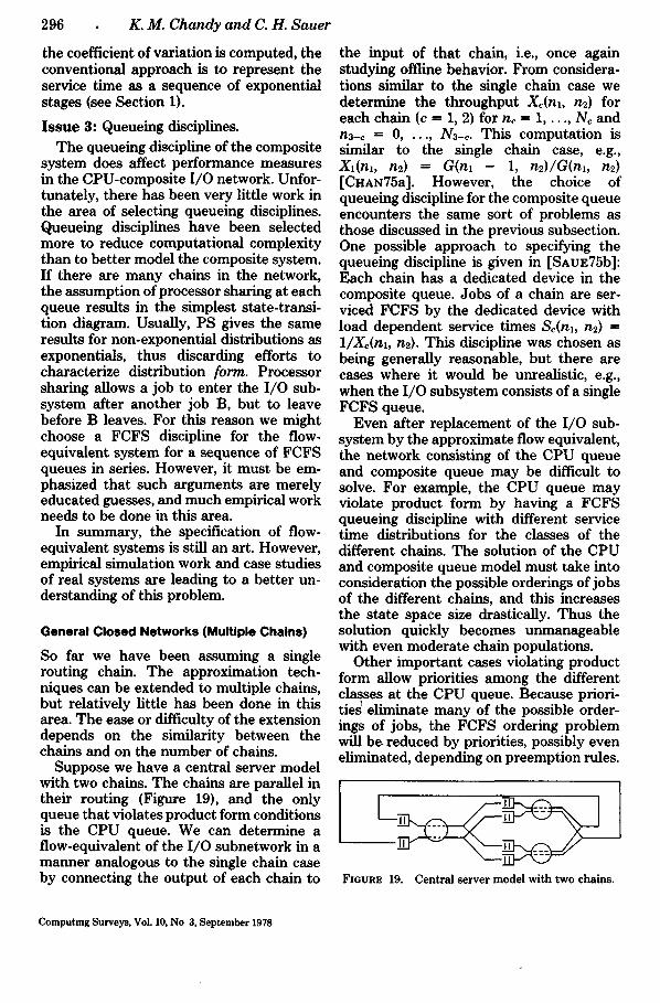
Suppose we have a central server model with two chains. The chains are parallel in their routing (Figure 19), and the only queue that violates product form conditions is the CPU queue. We can determine a flow-equivalent of the I/O subnetwork in a manner analogous to the single chain case by connecting the output of each chain to

the input of that chain, i.e., once again studying offline behavior. From considerations similar to the single chain case we determine the throughput Xc(nl, n 2 ) for each chain (c ffi 1, 2) for nc = 1 . . . . , Nc and n 3 - c = 0 . . . . , N3-~. This computation is similar to the single chain case, e.g., Xl(nl, n2) ffi G(nl - 1, n2)/G(nl, n2) [CHAN75a]. However, the choice of queueing discipline for the composite queue encounters the same sort of problems as those discussed in the previous subsection. One possible approach to specifying the queueing discipline is given in [SAUE75b]: Each chain has a dedicated device in the composite queue. Jobs of a chain are serviced FCFS by the dedicated device with load dependent service times SAn1, n2) = 1/X~(nl, n2). This discipline was chosen as being generally reasonable, but there are cases where it would be unrealistic, e.g., when the I /O subsystem consists of a single FCFS queue.

Even after replacement of the I/O subsystem by the approximate flow equivalent, the network consisting of the CPU queue and composite queue may be difficult to solve. For example, the CPU queue may violate product form by having a FCFS queueing discipline with different service time distributions for the classes of the different chains. The solution of the CPU and composite queue model must take into consideration the possible orderings of jobs of the different chains, and this increases the state space size drastically. Thus the solution quickly becomes unmanageable with even moderate chain populations.

Other important cases violating product form allow priorities among the different classes at the CPU queue. Because priori- tie~ eliminate many of the possible orderings of jobs, the FCFS ordering problem will be. reduced by priorities, possibly even eliminated, depending on preemption rules.

~ - - - i i_j - J ~ _ 1

FXGURE 19. C e n t r a l s e r v e r m o d e l w i t h two cha ins .

Computmg Surveys, VoL 10, No 3, September 1978

But these cases also become unmanageable with moderate numbers of chains (e.g., five).

When the CPU-composite queue network becomes unmanageable because of chain populations and/or numbers of chains, one can attempt aggregation of chains as well as aggregation of queues. In aggregation of queues one replaces several queues by a composite queue that is approximately flow-equivalent as far as the remaining jobs are concerned. In aggregation of chains one replaces several chains by a single chain that is approximately equivalent as far as the remaining jobs are concerned. The approach used in [SAuE75b) is first to solve a central server model identical to the given model, except that the CPU queue with disciplines violating product form is treated as a processor- sharing queue. The service times at the I/O queues are the same for all chains, assuming FCFS disciplines at those queues. For the chain-dependent values (the CPU service time distributions and the routing frequencies) the "composite chain" values are determined as a weighted sum of those values for the componen t chains. The weights used in [SAuE75b] are the throughputs of the component chains divided by the sum of the throughputs of the component chains. Other weights may be used, e.g., the number of jobs of the component chains divided by the total population of the component chains [MAcN75].

These techniques extend to networks with more complex routing structures than the central server model; the appendix con- tains an example.

Flow-Equivalents in Simulation

Some of the subsystem flow-equivalents could be constructed from simulations, i.e., by simulating a subnetwork. We could also use simulation to analyze the model with the flow-equivalents. Note that flow-equivalent methods are totally general because the technique used in constructing flow- equivalents (e.g., simulation, queueing theory, regression analysis) is left unspecified. See [CHIU78, SAUE76, and SCHW78] for further discussion of this approach.


Justification of Aggregation

We informally described the class of product form networks in Section 1. At the beginning of this section we stated that aggregation was exact for product form networks, i.e., one can determine the flow- equivalent of a product form subnetwork and use the flow-equivalent in a product form network as if it were the given subnetwork. This should be plausible to the reader, since the state of a product form network factors into components representing the states of the queues of the network. Informally, aggregation of the queues corresponds to association of the factors. For a more formal discussion see [CHAN75a].

The primary justification we have im- plicitly used for aggregation approximation is the exact aggregation of product form networks. This justification becomes less credible as the network to be solved becomes "less similar" to a product form network. Examples include the number of queues violating product form conditions (e.g., distributions and disciplines) increasing, an individual queue tending to deviate greatly from product form conditions (e.g., service times at an FCFS queue having very small or very large coefficients of variation), and conditions such as multiple resource holding becoming dominant. There is another justification, loosely coupled subnetworks [CouR75, COUR77], which is independent of product form conditions. The product form justification holds regardless of the degree of coupling of subnetworks; the loosely coupled justification holds regardless of product form conditions.

We illustrate degree of coupling by an example. Consider a closed queueing network with two subnetworks A] and A2 (Fig- ure 20). A job leaving a subnetwork is fed back to the input of the same subnetwork with frequency p, and goes to the other

FmURE 20. Two loosely coupled subnetworks, p ffi 1.



subnetwork with frequency 1 - p. Consider the limiting behavior of this network as p tends to 1, but p < 1. The rate of flow of jobs between the subnetworks decreases as p increases, which implies that the times between subnetwork interactions (job transitions) increase. In the limiting case of p arbitrarily close to but less than 1, each subnetwork may be assumed to reach equilibrium between subnetwork interactions. This key idea will be developed further.

If p = 1 the network decouples into two closed networks BI a n d B2 (Figure 21) where B,, i = 1,2 is the network obtained by feeding the output of A, back to its input (Figure 20). Let there be C chains in the network and let Xc(nl, . . . , nc) be the equilibrium throughput of chain c jobs in Be when the population of B2 is n], ..., nc for chains 1 . . . . , C, respectively. Suppose we wish to study the detailed behavior of jobs within A]. Then we may replace A2 by a composite queue that has a mean service time of 1/((1 - p)Xc(n] . . . . . nc)) for class c jobs (at a device dedicated to class c) when the queue population is nl . . . . , nc. (The service distributions may be set to the in- terdeparture distribution in B2. It can be shown that as p approaches one the inter- departure distribution becomes exponential.) Decoupling works as p tends to 1.

Summary

The key concept in aggregation is to replace a subnetwork by a simpler one, ignoring the interactions of subnetwork components not of interest to us. In the terminology of Denning and Buzen [DENN78], we are assuming that the subnetwork's offline behavior is identical to its online behavior. The basic problem is to 1) develop a frame- work for characterizing the offline behavior, 2) solve the subnetwork to estimate these characteristics, and 3) aggregate the behav-

FIGURE 21. Decoupled subnetworks.

ior of subnetworks until we obtain a network with a tractable solution. We have assumed the concept of flow-equivalence as a solution to the first part of the problem and have illustrated approaches to the second and third parts by examples.

4. IMPROVEMENTS OF FLOW- EQUIVALENCE

The goal of flow-equivalence approximations is to simplify network analysis by replacing a subnetwork by a single composite queue that behaves in approximately the same way as the subnetwork. Further- more, the composite queue must have simple queueing disciplines and distributions to keep the computation manageable. In this section we shall survey methods that attempt to reduce the inaccuracies resulting from simplistic representations of subnetworks. Rather than attempting to represent a subnetwork accurately, these methods carry out the computation assuming simplistic subnetwork representation and later attempt to correct for the inac- curacy in subnetwork representation. We survey two such methods: iteration and product form. We next discuss the common aspects of these methods and then discuss the methods in detail. The key concepts used in the two methods can be combined.

An Overview of the Approaches

We partition a network A into subsystems S1 . . . . . S• in some suitable manner. Since we analyze each subsystem in turn, we would like to keep the number M of subsystems small. On the other hand, we do not want a subsystem to be so complex that analyzing it by itself becomes an unmanageable problem. We analyze each subsystem S,, i = 1, ..., M in the following way. Define (7,, the complement of S,, to be the subnetwork obtained by removing S~ from network A. C, is the system "seen" by S,. Represent each system C, by a single composite queue F,. Analyze the network consisting of S, and F, by some suitable method; the specific method selected depends upon the complexity of S, and F,. If a simple service rate structure (such as


rates proportional to the number of jobs in the system) is assumed for the flow-equivalent system, it may be possible to get exact closed form formulas for the performance measures of the F, - S~ network; indeed, such simple solutions are the motivation for simple (approximate) rate structures for F,. For general service rate structures, the F, - S, network may be modeled as a Mar- kov process and analyzed by a recursive method, by sparse matrix techniques, or by simulation. Since the F, are approximations to the C,, the results of the analyses of the F, - S, networks will generally be inaccurate; informally speaking, the less accurate the representation of the C, by the single queues F,, the greater the error.

One consequence of this error is that the estimates of the performance measures for Sl, . . . , SM computed from the F, - S, analyses may not be compatible with each other. For instance, assume that we compute the rate of flow of jobs through each subsystem S, by analyzing the F, - S, network. By multiplying the flow rate through S, by the probability that a job leaving S, will enter S~, we compute the rate of job flow from S, to Sj. We may now compute the total flow entering Sj by summing the flows over all paths into Sj. If the analysis were free from error the flow rate into Sj must equal the flow rate through S~. How- ever due to the approximations inherent in the analysis of each subsystem, the computed flow rates into S~ may not equal the computed flow rates through Sj.

We can use several rules to check the compatibility of the computed performance measures for S~, ..., SM. The more checks we use, the greater will be our faith in the compatibility of the results. However we may not wish to spend a great deal of computing time on the checking process. It must be emphasized that even though the computed subsystem performance measures satisfy some compatibility tests, there may still be errors in the computed measures.

The fundamental problem with computing performance measures for S~, ..., SM by the method discussed above is that the independent subsystem analyses emphasize the local view; i.e., the subsystem itself is


modeled in detail while everything else is modeled in a gross fashion. The compatibility checks take a global network view. Product form methods attempt to correct for the local views emphasized in the independent subsystem analyses by taking the specific global network view discussed next. Let p,(s~) be the value computed for the equilibrium probability that subsystem S, is in state s~ by analyzing the F, - S, network; note that thep,(s,) are probabilities local to subsystem S, - - the rest of the network is ignored. Letp(s l , . . . , SM) be the equilibrium that subsystem S, is in state s, for i ffi 1, .... M; note that p(sl . . . . , SM) takes a global network view because it is concerned with all the subsystems in the network. Product form methods assume that

1 p(s, . . . . . SM) = ~ n p,(s,) all s, . . . . . SM

where G is a normalizing constant. Thus the local subsystem analyses are forced into the global mold of the product form. Per- formance measures are now computed from the network probabilities, p(s l . . . . . SM) rather than from the subsystem probabilities p,(s,).

Product form methods are often combined with iterative methods; examples are provided later.

Iteration methods take the global view by making compatibility checks of the re- suits of subsystem analyses. If the checks are not satisfied, the single queue models (iv,) of the complements (C,) are modified; the specific method of modification depends upon the specific iteration method used. In the next iteration, the improved single queue models are used in the F, - S, analyses. The process of making compatibility checks and modifying composite queue models is repeated until the compatibility checks are satisfied.

There are two difficulties with this method. First, satisfying the compatibility checks is no guarantee of the correctness of the results. Second, there is no guarantee that the iterations will terminate. Yet, (perhaps surprisingly) iteration methods seem to work satisfactorily much of the time [CHAN75b, LAM76]. We discuss some specific iteration methods next.

Computing Surveys, Vol. 10, No 3, September 1978

300 K. M . C h a n d y a n d C. H . S a u e r

Iteration Methods

The questions we shall focus attention on are

• What are the subsystems that a network is decomposed into?

# What laws are used to check whether the subsystem analyses are compatible?

• What flow-equivalent models are used? • How are the independent subsystem

analyses adjusted if the results from these analyses are incompatible?

The laws that we use in checking the compatibility of the computed subsystem measures are called i n v a r i a n t s . We now discuss three different cases where iterative methods have been used.

General Closed Queueing Networks

We summarize the method described in [CHAN75b]. Two invariants are used in this method.

1) The rate of flow of chain c jobs into a subsystem must equal the rate of flow of chain c jobs out of that subsystem.

2) If chain c is a closed chain, the sum of the mean number of chain c jobs in subsystem S,, summed over all i, must equal the total number of chain c jobs in the network.

We now present some details of the algorithm assuming a closed network with a single closed chain of jobs. Extending the method to multiple job chains is straightforward. {Examples of a closed network with two job chains and of an open network are presented later in this section.) Let it, be the mean queue length of queue i. Com- pute a set of numbers y,, which we call relative throughputs, where

M yj ffi ~ Y,q,J

t m l

Note that the y, are unique up to a normalizing constant. Let tj be the throughput through the j th queue. Since the flow into queue j is equal to the flow out of queue j,

tj = ~, t,q,j. Invariant I; Flow Invariant 1

Hence we have t j f a y ~ for allj,

where a is a constant. Set t / ffi t f f yj ;

we refer to the t / as the n o r m a l i z e d throughputs. An equivalent formula for the first invariant is

t]' ffi t2' ffi . . . ffi tM' ffi t' Flow Invariant

where t ' = Z t , ' / M

i

is the average value of the normalized throughput computed by analyzing all the queues independently.

The second invariant is

Y~ ri, ffi N Invariant lI; Population Invariant I

where N is the population of jobs.

T h e C o m p o s i t e Q u e u e F,

We construct F, in the following way. Ideally, we would like F, to be the flow- equivalent of C,. However, to determine the flow-equivalent for C, we have to analyze C,. Analyzing C, may be a very expensive computational procedure if C, does not satisfy product form. Hence, we are forced to settle for making F, an a p p r o x i m a t m n to the flow-equivalent of C,. This approximation is obtained by computing the flow- equivalent for C, a s s u m i n g (generally in- correctly) that C~ satisfies product form.

Note that we use two levels of approximation here. First, the F~ are not the true flow-equivalents. Second, even if the F, are the true flow-equivalents for C,, this heuristic may not yield correct answers.

I t e r a t i o n

On the kth iteration the service rates of F, are set equal to the service rates of the flow-equivalent of the complement of queue i in an auxiliary network S ~k). The auxiliary network is identical to the given network except that:

1) The service rates in the auxiliary network are different; and

2) The queueing disciplines in the auxiliary network are such that the network satisfies product form. Hence the flow-equivalents for the complement of any queue in the network can be readily computed.

The goal of the iteration is to adjust the

Comput ing Surveys , Vol 10, No 3, S e p t e m b e r 1978

flow rates of the auxiliary network (which results in adjustments to the F~ and consequent changes in queue statistics), so as to force the individual queue statistics towards satisfying the invariants. The details of this adjustment are not presented here; they may be found in [CHAN75b]. If the invariants are not satisfied the results of the iterative method are incorrect; however, if the invariants are satisfied it does not necessarily mean that the solutions are correct. Nevertheless, this approach has been validated by comparing the results obtained by this method with results obtained from simulations for several cases. Networks with several chains of jobs and a variety of queueing disciplines (including priority disciplines) were analyzed by this method. For details regarding the algorithm, its accuracy, and execution times, the reader is referred to [CHAN75b].

A Case Study for VM/370 Using IteraUve Methods

We next discuss an iterative scheme proposed for modeling scheduling strategies for interactive computers [BARD77]. This work is important for several reasons. The scheme itself is very simple, and therefore appealing. Furthermore, the method has been used to model the effects of workload and configuration changes for a widely used complex interactive operating system, VM/ 370. It has been incorporated into a performance package for configuring VM/370 systems as discussed in [BARD78] (See pp. 333-342, this issue).

We shall summarize the results in [BARD77], restricting attention to the prin- ciples of constructing an iterative method.

A user is assumed to make transitions between states in a cyclic fashion: THINK - MEMORY-WAIT - ACTIVE- THINK-. . . , or equivalently 1, 2, 3, 1 . . . . .

For purposes of exposition assume that there are only two job chains:

Chain 1: trivial jobs Chain 2: non-trivial jobs.

A trivial job is assumed to be immediately admitted to service, i.e., it is assumed to spend no time in the MEMORY-WAIT state. Thus its state transitions are


THINK-ACTIVE-THINK, ..., or 1,2,1, . . . . A non-trivial job may have to spend time in the MEMORY-WAIT state. The diagram for the overall system is shown in Figure 22.

Model inputs: We are given the number of jobs N, in chain i; the mean main memory requirement (resident set size) W, for jobs in chain i; T,, 1, the mean think time (i.e., time in state 1 for chain i jobs), and S, the total amount of main memory available. We are also given details regarding the visit counts and mean service times at the CPU and I/O devices for both chains.

Model outputs: We are required to compute T,, 2 and 7',,3, the mean times spent by chain i jobs in state 2 (MEMORY-WAIT) and state 3 (AC- TIVE). We shall also compute N,.k, the average number of chain i jobs in state k, k = 1, 2, 3, and St the mean amount of main store occupied by all the chain i jobs together.

Aggrega t ion : The model is analyzed into two stages. In the first stage the computer subsystems representing jobs in the active state (Figure 23) is analyzed. The mean time T,. 3 spent by chain i jobs in the active state is computed from this submodel (see below).

The overall model is analyzed in the second stage (Figure 24). Note that in this stage, the computer subsystem is represented as a flow-equivalent server with in- finitely many servers, which is equivalent to a delay of T~, 3 time units.

Invariants: The probability P~k that a random chain i job (i = 1, 2 for trivial, non- trivial) is in state k (k ffi 1, 2, 3 for think, memory-wait, and active) is proportional to the time spent by that job in that state, i.e.,

T~,k P,k = for all ~, k

T~.I+ T,.2+ T~,3

Hence the mean number of chain i jobs in state k is

Invariant 1

N,.kffiN, P ,h fN , T,,~+ T,,~+ T,,3"

Computing Surveys, Vol 10, No. 3, September 1978


THINK STATES

Chain 2:

Non- Trivial Jobs

Chain 1:

Memory Wait Queue

, F I

Tr i v i a l Jobs!

: Svstem~'~l I ' '

i_ _J

I A1 locate Memory

J Rel ease Memory

FICURE 22. Interactive system.

FmURE 23. Computer subsystem.

lnvariant 2 T h e mean amount of main storage used

by chain i jobs (S,) is the product of the average number of chain i jobs in main storage (N,, 3) and the average amount of main storage required per job (W,).

S, ffi N,,3. W,.

Note tha t T~, 2, the t ime spent by a trivial job in the memory-wa i t state, is 0 {zero). Hence

Tl, a $1 ffi Wl Nl. T1.1+ T1,3"

Note tha t we are given N1, W1 and T~, 1. If we are given T~, 3 then we may compute S~

from the above equation. If $1 -< S then there is enough main store to accommodate trivial jobs, and our assumption of T1, 2 = 0 is reasonable; if $1 :> S the system is satu- ra ted by trivial jobs, and we must stop our analysis.

T h e above arguments are not strictly correct because they are based entirely on mean values, ra ther than distributions. Strict ly speaking, a trivial job will experience memory-wa i t if all of main storage is filled with o ther trivial jobs; the only case when this si tuation will never occur is when

NI W I ~ S

ra the r than N1,3 Wl <-- S.

However, the goal here is not to come up with a mathemat ica l model but ra ther to develop a heuristic program tha t seems to work most of the time. Th e only test for such heuristics is validation.

We may develop a similar invariant for chain 2 jobs. If we assume T2, 2 ffi 0, i.e., the

Computing Surveys, Vol 10, No 3, September 1978

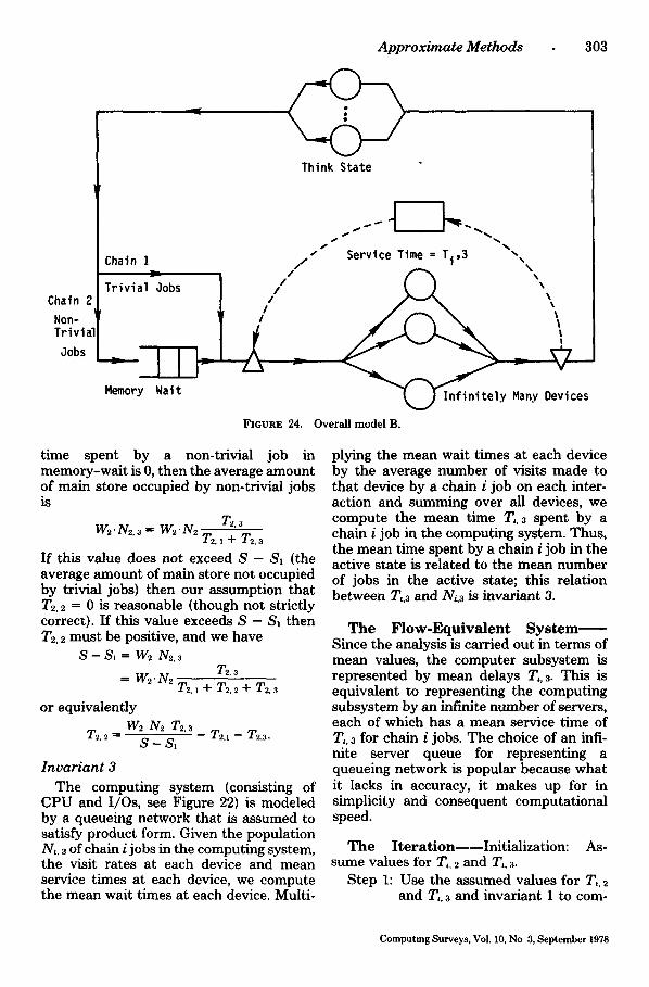
Chain 1 /

Trivial Jobs I / Chain / Non- Trivial

Jobs J[ =-

Memory Wait

FIGURE 24.

A p p r o x i m a t e M e t h o d s

Think State

, s s

Service Time = Ti,3 x x

~..~) In f in i te ly Many Devices

Overall model B.

303

time spent by a non-trivial job in memory-wait is 0, then the average amount of main store occupied by non-trivial jobs is

T2,3 W2.N2,3 ffi W2.N2 T2.1 + T2.3

If this value does not exceed S - S~ (the average amount of main store not occupied by trivial jobs) then our assumption that T2, 2 = 0 is reasonable (though not strictly correct). If this value exceeds S - S~ then T2, 2 must be positive, and we have

S - S 1 = W2 N2,3

ffi W2"N2 T2,3 T~ , l+ T2.2+ T2.3

or equivalently W2 N2 T2, 3

T~. 2 = T2,1 -- T~,3. S - $1

I n v a r i a n t 3

The computing system (consisting of CPU and I/Os, see Figure 22) is modeled by a queueing network that is assumed to satisfy product form. Given the population N,, 3 of chain i jobs in the computing system, the visit rates at each device and mean service times at each device, we compute the mean wait times at each device. Multi-

plying the mean wait times at each device by the average number of visits made to that device by a chain i job on each interaction and summing over all devices, we compute the mean time T,, 3 spent by a chain i job in the computing system. Thus, the mean time spent by a chain i job in the active state is related to the mean number of jobs in the active state; this relation between T,,3 and Ni,3 is invariant 3.

The F low-Equiva len t Sys tem Since the analysis is carried out in terms of mean values, the computer subsystem is represented by mean delays T,. 3. This is equivalent to representing the computing subsystem by an infinite number of servers, each of which has a mean service time of T,, 3 for chain i jobs. The choice of an infinite server queue for representing a queueing network is popular because what it lacks in accuracy, it makes up for in simplicity and consequent computational speed.

The Iteration----Initialization: As- sume values for T,, 2 and T~, 3.

Step 1: Use the assumed values for T,, 2 and T,, 3 and invariant 1 to corn-


304

Step 2:

Step 3:

Step 4:

K. M. Chandy and C. H. Sauer

pute N,, 3, which is the job population assumed in the computer subsystem. Use the N,. 3 obtained in step 1 with invariant 3 to recompute T~,3. Use T,, z obtained in step 2 with invariant 2 to recompute T,. 2. Return to step 1 with new values for T,. 2 and T,. 3, if there is a significant difference between the old and new values. Other- wise, stop.

This method has been validated and is in use. It cannot be overemphasized that the credibility of a heuristic technique rests on empirical validation rather than on logical rigor. Bard's method [BARD77] is credible because it has worked for several practical cases, even though there is no guarantee of convergence and the analysis is informal, being based on mean values. Systems analysts are also more likely to have faith in a model, such as Bard's, that considers key parameters, such as amount of main memory, memory scheduling, different kinds of users, and the complex queueing structure of I/O channels. The method has a computation time favorable to that of other methods (such as simulation) and satisfactory accuracy. There is no point in developing an algorithm that invests a great deal of computer time in obtaining a degree of accuracy that is greater than is required for making the decisions at hand.

An IteraUve Scheme for Open Network Models of Packet-Switching Systems

We now discuss the use of iteration techniques in the analysis of communication networks [LAM76]. This discussion is important for three reasons. First, communication systems are important in themselves. Second, this section illustrates the use of heuristic approaches in modeling finite waiting rooms. Third, this section provides an example of approximation methods usecl to analyze open queueing network models. (See also [WONG78] pp. 343-351, this issue.)

A job in this context is a "packet," which is a basic unit of communication. The system accepts packets at sources, routes them

through communication lines and switches, and delivers packets to destinations. The resources in the system are communication lines, the switches which route packets along appropriate paths, and the memory (store and forward buffer) at each switch in which packets are stored until they can be shipped out along appropriate communication lines. The servers in the queueing network model are the communication lines and the switches. However, since the actual service time of a switch is small compared to the service time at a communication line, we shall ignore switch service times.

Associated with each packet is a source node and a destination node. A packet moves through the network from the source node to the destination node along a fixed route. The ith node of the network has a finite number N, of store and forward buffers, i.e., it has a finite waiting room. If there are N, packets in the ~th node when another node k tries to send one more packet J to the ith node, then the ith node refuses to accept J, and J must be retrans- mitted by node k. In other words, a server at node k serves J, and if at the instant at which J completes service the waiting room for node i is full, then the server repeats J 's service, until eventually there is a vacant position in i's waiting room.

Figure 25 is a queueing model of one node of the network {node i). This node is assumed to communicate directly with I other nodes, ~1, . . . , il. We also use one "dummy" node, /0, to represent users who send and receive packets directly from node i. We assume that all lines are full-duplex, i.e., that packets can be transmitted in both directions simultaneously. There are I + 1 parallel servers associated with node i, and the j th such server, j ffi 0, 1 . . . . , I models the communication line from r, ode i to node ij; this server serves those packets in the node i waiting room that have to go to node ij. Even if all service times are assumed to be independent exponential random variables, this queueing network does not satisfy product form because of the finite waiting room and the consequent retransmis- sion (re-serving) of jobs. Hence we shall resort to iterative approximation methods.

The network is partitioned into subsystems, one subsystem for each node. We


source


flow rejectant by i.~j due actual flow to to blockina _ ~ node ij

flow a c c e p ~ by node i 7 "

/ ~ . channel from i to ij

Dr~I~Y Bifl!w rejected

", FIGURE 25. Network model for node t.

next discuss the key questions which arise in iterative methods.

I n v a r i a n t s : Let hu be the apparent flow rate of packets (i.e., not including retransmissions) from node i to node ij. We can compute the hu from the rate at which packets enter the network and the routes taken by packets as they travel from the source to the destination. Let r,j be the actual flow rate of packets (i.e., the apparent flow plus retransmissions) from node i to node ij Let Bj be the probability that the waiting room at node ij is full. Then r u. (fraction of time the node j

waiting room is not full) = ,k,~

i.e., r u = ~u/(1 - B~) Invartant 1

Let gu be the service rate of the channel from node i to node ij. Assume product form for the queue length distribution of each channel. This assumption is invalid due to the finite waiting rooms. However, we make this assumption to make the corn-

putation manageable. The probability tha t there are qu packets at node i waiting to be shipped to node j is:

Pu(q,~) = Pu(0) ' (r,Jpu)qu

Now assume product form for the entire tth node. This is also an invalid assumption tha t is made to make the problem manageable. Then, the equilibrium probability tha t there are q,j packets at node t going to node ij, j - 0, 1 . . . . . I i s

P,(q,o . . . . . q,l) = H p,J(q,J) Invariant 2 y

Thus Invariant 2 is a relationship between actual flow rates and node state probabilities.

I n v a r i a n t 3

The probability B, tha t the node i waiting room is full is the sum of the probabilities P, (q,.0, . . . , q,, ~) over all states with q,.0 + . . . + q,.~ = N,.

Thus the blocking probability B, depends upon (Invariant 3) the state probabilities p,, which depend upon (Invariant 2) the



actual flow rates r,j, which depend upon (Invariant 1) the blocking probabilities Bj. In this formulation, the flow-equivalent of node i is defined in terms of the blocking probability B, and the flows ~j, and ~ , j into and out of i.

I t e ra t ion : A simple iterative scheme is to assume a set of blocking probabilities Bj and to then use Invariants 1, 2, and 3 in that order to get a new set of blocking probabilities. This iteration is repeated until successive iterations do not produce a significant change in blocking probabilities.

The networks described here may en- counter deadlocks. In this case the equilibrium throughput is 0 (zero) and the above analysis is wrong. However, the results computed by the iterative method proposed here are meaningful (though not mathematically correct) if the probability of deadlock is low. In this case, the performance measures predicted by the model should be taken to be the values that occur after the network has been in deadlock-free operation for a long time.

Product Form Methods

Reiser and Kobayashi [REIs74] use product form approximations; their method is discussed in Section 6 in connection with diffusion approximations.

Shum and Buzen [SHUM77] couple the product form method with an iterative scheme in an interesting fashion. Their goal is to analyze closed queueing networks with general service time distributions and FCFS queueing disciplines. We shall discuss their technique in the same format as other iterative techniques.

Aggrega t ion : Each queue is analyzed independently. The complement C, of the ith queue is represented by a single queue F, with a load independent service rate and exponential service times. This is obviously a very simplistic model for the complement. However, the product form and iterative prodecures attempt to correct for the inac- curacy in subsystem representation.

As in all product form methods, the equilibrium state probabilities for the entire network are computed by taking the product of the state probabilities for each queue

that are computed from analysis of the S, - F, networks. Performance measures are computed from the state probabilities of the entire network (rather than from subsystem state probabilities).

Invariants: The first invariant used in [CHAN75b] is alSO used here: flow rate into a queue must equal flow rate out of that queue. This scheme uses a single invariant.

Iteration: The algorithm iteratively ad- justs service rates of the composite queues F, until the flow invariant is satisfied. The flow invariant states that all queues must have the same normalized throughput (see 4, General Closed Queueing Networks). Let t', be the normalized throughput of queue i. The flow invariant is satisfied when

t ' l - - t ' 2 . . . . . t'K. To measure how closely the normalized throughputs computed at any point in the algorithm satisfy the flow invariant, the following error function is used.

K

L = T. (y , / /L , ) • ( t ' , - t * ) 2 i l l

where y, is the relative visit rate into queue i. p, is the service rate of queue i and hence y,/#, is proportional to the utilization of queue i. t* is the normalized throughput of the queue with the highest utilization. The above error function is used because the "bottleneck queue" (i.e., the one with the highest utilization) plays a crucial part in calculating queue statistics. The error function also gives greater weight to queues with greater utilization.

Let k, be the service rate of the composite queue F,. Let

~, = ky, a n i

where k is an (unknown) constant. Assume an initial value for k and at each step of the iteration adjust k to minimize the error function L.

Summary

Two questions must be asked about these iterative methods:

1) Do these methods give more accurate estimates of key performance measures than straightforward flow- equivalent approaches?


2) If these methods do give more accurate results, is the increased accuracy worth the additional computational effort?

These questions cannot be answered cat- egorically. There are cases where a relatively straightforward flow-equivalent approach is more accurate than the iterative methods, and cases where the iterative methods are more accurate. However, it is our opmton that the methods discussed in this section generally improve upon the results of direct flow-equivalent methods; this opinion is based upon case studies, including those surveyed in this section.

The ubiquitous tradeoff of improved accuracy versus greater computational effort can only be resolved by studying the specific requirements of the problem at hand and by comparison with alternate methods such as simulation.

5. FLOW-EQUIVALENT SYSTEMS AND THE MANAGEMENT OF MODELING PROJECTS

Performance modeling projects of actual or proposed systems are usually carried out under intense time pressure. The largest portion of time by far is spent on understanding the system to be modeled: poring through documentation and talking to system designers. It is crucial to divide the work to allow several modelers to work together with minimum conflict. A solution used by Browne, et al. is based on the chief programmer-team approach used success- fully in the development of large programs [BROW75]. This discussion is a summary of their solution.

The chief modeler (in analogy to the chief programmer) partitions the overall system model into logically consistent subsystem models and assigns each subsystem to a different member of the modeling team. Examples of subsystems in the study of the Air Force Logistics computing system include the CPU subsystem, database management, disk subsystem, and the tape subsystem. Each member of the modeling team is expected to become an expert on his subsystem, interact with the appropriate system designers, and eventually construct a flow-equivalent system model (or a range of such models) for his subsystem.


The chief modeler should partition the overall model into subsystems so that, as far as possible, the subsystems are independent of each other. For reasons of clarity it is helpful to focus attention first on subsystem disciplines (e.g., priorities) and later consider details about the job mix {e.g., map chains and job classes to priorities). The chief modeler is responsible for checking that the flow-equivalent models of the subsystems are reasonable, putting the subsystem models together, and evaluating the overall model. Browne, et al., refer to the models required to produce flow-equivalents as micro-models and to the overall model consisting of a network of flow- equivalents as a macro-model. Note that the complexity of the micro-model may be greater than that of the macro-model.

A large simulation program was also constructed in this parallel fashion by the chief modeler-team. Browne, et al. report good results from this management technique. Though they use a two-level hierarchy (chief modeler and his team) there is no reason that the method of flow-equivalents could not be used with a deeper hierarchy. The general question of how much error is introduced by this hierarchical technique is still open.

The problem of managing large-scale modeling projects has received very little attention; this problem is likely to become acute. (See COUR77.)

6. DIFFUSION APPROXIMATION

Diffusion approximation methods use the theory of diffusion processes to analyze queueing problems. The reader need not be scared by the wealth of literature on diffusion processes, or by the apparently difficult mathematics involved in the development of the theory of diffusion. Most users merely use formulas from the diffusion approximation literature without understanding the detailed development of the formulas. Indeed, it is not necessary to understand the development of the formulas, provided that empirical studies show that the formulas fit experience. The only cases in which the systems analyst needs a thorough understanding of the mathematics of diffusion is when attempting either to develop



better approximations [GELE75] or to extend the approximations to new problems [Fosc77]. The following section is directed toward the large majority of analysts who need some understanding of diffusion approximations, but who are unlikely to attempt research in the area.

The organization of this section is as follows: we 1) discuss diffusion processes from a very informal point of view; 2) discuss the problem of mapping queueing processes onto diffusion processes; 3) review studies on the accuracy of the diffusion process; and 4) finally attempt to see where diffusion approximation techniques fit into the general scheme of queueing network analysis.

Why Bother with Diffusion Processes?

To illustrate the need for diffusion approximations consider a GI/G/1 queue, i.e., a s!ngle server queue fed by a job source where service and interarrival times are independent random variables having arbitrary general distributions. {Note that diffusion approximation methods are not restricted to GI/G/1 queues.) Let n(t) be the number of jobs in the queue at time t. n(t) can take on the values 0, 1, 2 . . . . We may think of n(t) as the position of a particle d (for discrete) that makes a jump (of + 1) to the right when a job arrives and a jump (of - 1) to the left when a job departs (Figure 26). In general, the probability that d will

• ovement of ~arttc~e d

÷1 +1 *1 ~1 ~ (t)

-1 -1 -1 -1

m o v ~ n t of na r t ; c l e d •

p] ice d* ~fl o o s i t t o n ~ ~ e n

x

i n te rva ls

movesent of p a r t i c l e c (d i f f us ion )

FmuRlg 26. Modeling p ~ m l e d by particle d*.

make a jump of + 1 or -1 in the next incremental time interval depends upon d's past behavior. For example, the length of time that d will stay in its current place (in general) depends upon the time since the last arrival or departure.

Our goal is to deduce the probability of d's future behavior given its past behavior. A conventional approach is to represent (possibly approximately) the service time and the interarrival time by a finite collec- tion of exponential stages (Section 1). All the" relevant information in a queue's past behavior that is required to predict the queue's future behavior is captured by the "state" of the queue. The state-transition (differential) equations may be solved to obtain state probabilities as a function of time from which we can compute the probability that particle d is in position n at time t. Since there are an infinite number of states, this computation is not carried out numerically; if it can be carried out at all the computation is done algebraically. If we are dealing with a finite job population it may be possible to carry out the computation numerically, but we may prefer a less expensive approach such as the diffusion approximation. Thus we attempt to use d~f- fusion approximations only when numerical and algebraic methods fail.

The difficulty with predicting the behavior of particle d is that it has memory in addition to its current position, i.e., the state of the system is not merely the particle's current position. (The analogy to the GI/G/1 queue tells us we must remember the residual service time.) In the diffusion approximation, we model the behavior of particle d approximately by the behavior of a particle c (for continuous) where c has no memory.

Whereas d can only take on values 0, 1, 2 , . . . , we let c take on all values on the non- negative real line. Let us now decide how c should move along the real line. Since we are used to dealing with discrete state spaces we shall treat the continuous state space of c as the limiting case of a discrete state space. The discussion here is an informal treatment of material in Cox65.

Assume that particle c can only move at times 0, T, 2T, 3T, . . . . where T is some

Computing Surveys, Vol 10, No 3, September 1978

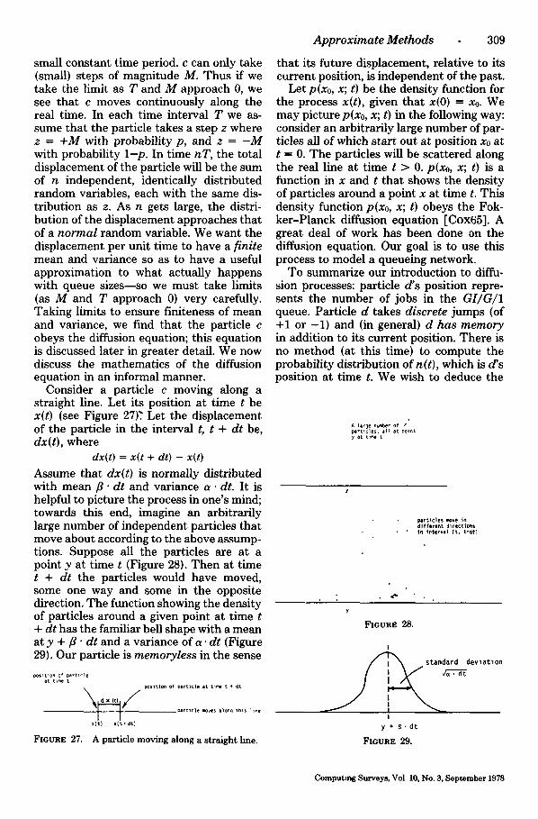
small constant time period, c can only take (small) steps of magnitude M. Thus if we take the limit as T and M approach 0, we see that c moves continuously along the real time• In each time interval T we assume that the particle takes a step z where z ffi +M with probability p, and z -- - M with probability 1-p. In time nT, the total displacement of the particle will be the sum of n independent, identically distributed random variables, each with the same distribution as z. As n gets large, the distribution of the displacement approaches that of a n o r m a l random variable. We want the displacement per unit time to have a f in i te mean and variance so as to have a useful approximation to what actually happens with queue sizes--so we must take limits (as M and T approach 0) very carefully. Taking limits to ensure finiteness of mean and variance, we find that the particle c obeys the diffusion equation; this equation is discussed later in greater detail. We now discuss the mathematics of the diffusion equation in an informal manner.

Consider a particle c moving along a straight line. Let its position at time t be x(t) (see Figure 27)." Let the displacement of the particle in the interval t, t + d t be, dx( t ) , where

dx(t) = x(t + dt) - x(t)

Assume that dx( t ) is normally distributed with mean fl • d t and variance a •dt . It is helpful to picture the process in one's mind; towards this end, imagine an arbitrarily large number of independent particles that move about according to the above assumptions. Suppose all the particles are at a point y at time t (Figure 28). Then at time t + d t the particles would have moved, some one way and some in the opposite direction. The function showing the density of particles around a given point at time t + dt has the familiar bell shape with a mean at y + fl " d t and a variance of a" d t (Figure 29). Our particle is m e m o r y l e s s in the sense

~sltlon of oartlcle at t i m e t + dt

x(t) x(t* dr)

FIGURE 27. A particle moving along a straight line.


that its future displacement, relative to its current position, is independent of the past.

Let p(xo, x; t) be the density function for the process x(t), given that x(0) --- x0. We may picture p(xo, x; t) in the following way: consider an arbitrarily large number of particles all of which start out at position xo at t ffi 0. The particles will be scattered along the real line at time t > O. p(xo, x; t) is a function in x and t that shows the density of particles around a point x at time t. This density function p(xo, x; t) obeys the Fok- ker-Planck diffusion equation [Cox65]. A great deal of work has been done on the diffusion equation. Our goal is to use this process to model a queueing network.

To summarize our introduction to diffusion processes: particle d's position represents the number of jobs in the G I / G / 1 queue. Particle d takes discre te jumps (of +1 or -1) and (in general} d h a s m e m o r y in addition to its current position. There is no method (at this time) to compute the probability distribution of n(t) , which is d's position at time t. We wish to deduce the

A IIrge nLh~nber of /' partlcles, i11 at Dolnt y at tt~ t

~rtlcles ~ve in d i f f e r e n t d~rectlons

• in Interval { t , t+dt]

Y

FIGURE 28.

I

standard devlat~on

• dt

!

y+B.dt

FmURE 29.


310 K. M. C h a n d y a n d C. H. S a u e r

behavior of d from the behavior of particle c that has simpler properties. Particle c moves along the con t inuous real line. Fur- thermore, c has no memory (except its position relative to the boundary). The position x(t) of c satisfies the diffusion equation, which has been studied in depth; methods exist to compute the probability distribution of x(t) . Note also that t rans ien t {time dependent) analysis of the behavior of c is tractable.

Mapping Between Queueing and Diffusion Processes

We wish to deduce the behavior of particle d from the behavior of particle c. To do this, we shall simulate the behavior of d by a particle d* that also jumps between points 0, 1, 2, . . . but whose movement is driven by the movement of c, in the following way. Partition the real line into intervals; place d* in position i when c is in the ith interval. When c moves to the i - l t h (or i+lth) interval, move d* to position i -1 (or i+1). Statistics regarding d* are said to be diffusion approximations of the corresponding statistics regarding d.

The accuracy with which d* models d depends upon:

1) How values are assigned to the parameters a and fl that characterize the diffusion process (and hence characterize the movement of particle c).

2) How the real line is partitioned into intervals (recollect d* is placed in the ith position when c is in the ith interval).

3) How we place a boundary condition on the diffusion process; typically we want c to move on the non-negative real line just as d does. There are different conditions we might place at the boundary x ffi 0 so as to ensure x(t) >_ 0 for all t. These boundary conditions affect the behavior of c and thus also the behavior of d*.

We shall analyze each of these issues in turn.

Setting a and f l

To make the computation of a and fl tractable we shall make the (invalid) assumption

that the queue is never empty. This assumption is more reasonable in "heavy traffic" conditions when the server's utilization approaches i (one), and the diffusion approximation tends to give better results under heavy traffic conditions.

Consider an incremental time interval [t, t + dt]. Let n(t) be the queue length at time t. During this interval the expected number of jobs to arrive is k . dt where ?, is the arrival rate and the expected number of departures is g" dt, where/~ is the service rate. Hence

E[n(t + dt) - n(t)] = (~ - #) •dt

We want the position x(t) of particle c to reflect the queue length n(t). Note from the earlier discussion that the incremental displacement x ( t + dt) - x(t) is a random variable with a mean of fl • dt. Hence, it is reasonable to set:

f l f f i ~ - ~

By similar (though more complex) arguments we set:

a ffi c~ + ca#

where ca and c, are the squared coefficients of variation of the interarrival and service times respectively.

Selecting Intervals

A reasonable heuristic is to place d* in the ith position when c is between i and i + 1 (Figure 26). Using this method of selecting intervals,

f ,+l P*(no, n;t) ffi P(xo, x;t)dx

Boundary Conditions

The reflective barr ier is the boundary condition normally used [Cox65]. This boundary condition states that the particle c must always be on the non-negative portion of the real line.

fo ® t)dx ffi 1 p(xo, x;

The diffusion equation with this boundary condition has been solved and we can compute p*(no, n; t). We are primarily inter- ested in the equilibrium queue length distribution:


p*(n) = p*(n0, n, oo)

Using the methods discussed previously for setting a and fl, the boundary condition, and for selecting intervals, we get ([GAVE68])

p*(n) = (1 -- ~)" ~n, n = 0, 1, 2 . . . . (6.1)

where ~ = exp {-2(1-p)/(c~ + cap)} and p is the utilization. Let p(n) be the equilib- r ium probabil i ty of n jobs in queue. We know tha t the fraction of t ime the server is idle is p(0) = l - p , whereas we have p*(0) = 1-~, which is erroneous. Hence a good heuristic is to use another approximation:

~b(n) = /1 - p if n = 0 (6.2) ( p" (1 - ~) ~"-; if n_> 1

Gelenbe uses a more reasonable boundary condition [GELE75]. He assumes that when particle c hits the boundary x = 0, it sticks there for an exponentially distr ibuted t ime after which it jumps back instantane- ously into the region x > 0 with some probabil i ty density function. For instance, we may assume tha t c makes an instanta- neous jump from x = 0 to the point x = 1, representing the arrival of a new job. We may assume tha t the mean t ime the process remains at the boundary x = 0 is 1/2,, where h is the arrival rate. With these assumptions Gelenbe reports improved results.

Networks

Consider a network with a single chain of jobs and K queues. Let n, be the number of jobs in queue i, i = 1, . . . , K, and let p(n], . . . . nK) be the equilibrium probabil i ty obtained by the diffusion approximation tha t there are n, jobs in queue i, i ffi 1 . . . . , K. In the pioneering work on networks by Ko- bayashi it was shown that given the usual assumptions for setting up the diffusion process,

~(n~ . . . . . nK) = ~ ~(r~) (6.3)

where G is a normalization constant for closed networks, and G = 1 open networks [KOBA74]. Note the product form of the network state probabilities.

For open networks we may estimate the coefficients of variat ion of the arrival process into each queue by the methods dis-

Approxtmate Methods 311

cussed earlier in Sect ion 3, and then analyze each queue independent ly assuming independent interarrival times with the estimated coefficient of variat ion and the specified arrival rate. Th e flow-equivalent of the complement is represented by a job source tha t has independent identically distributed service times.

For closed networks, Reiser and Kobay- ashi [REIs74] use the product form method discussed in Section 4. With this method we analyze each queue independent ly assuming a (simple) model for the complement of the queue, compute ft,(n,), and then use equat ion (6.2) to compute steady-state probabilities. We then compute network state probabilities assuming product form. Performance est imates are computed from the state probabilities ~6(nl . . . . . nK) ra ther than directly from the ti~(n,). For closed networks (unlike open networks), it is not possible to determine the arrival ra te into a queue without carrying out a detailed analysis of the entire network. One solution is to est imate arrival rates (or, equivalently, throughputs) assuming exponential service times, and hence product form, and to then use the formula (6.2) for single server queues.

An al ternative solution to estimating the arrival rates is to assume tha t the server with the highest utilization in the network is busy all the t ime (i.e., its utilization is 1) and then the th roughput (arrival rate) of tha t queue is equal to its service rate; the throughputs for all o ther queues can be computed from any one throughput [DENN78]. This al ternative method for es- t imating arrival rates is appropriate when the number of jobs in the network is very large.

Other Applications of the Diffusion Approximation: an Example

Foschini uses the diffusion approximation to solve routing problems [Fosc77]. Con- sider a system with a single source and two or more parallel queues (Figure 30). An arriving job joins the shor ter queue. This system has no simple analytic solutions. Foschini has an ingenious application of the diffusion approximation to this problem;


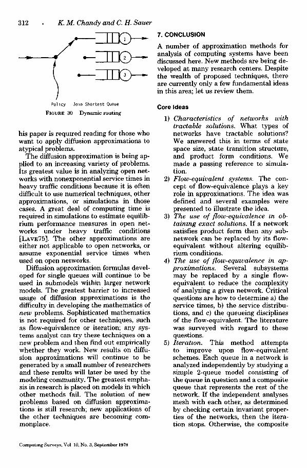
312

r

K. M. Chandy and C. H. Sauer

v v

P o l "~ cy

FIGURE 30

Joln Shortest Queue

Dynamic routing

his paper is requ]red reading for those who want to apply diffusion approximations to atypical problems.

The diffusion approximation is being applied to an increasing variety of problems. Its greatest value is in analyzing open networks with nonexponential service times in heavy traffic conditions because it is often difficult to use numerical techniques, other approximations, or simulations in those cases. A great deal of computing time is required in simulations to estimate equilibrium performance measures in open networks under heavy traffic conditions [LAVE75]. The other approximations are either not applicable to open networks, or assume exponential service times when used on open networks.

Diffusion approximation formulas developed for single queues will continue to be used in submodels within larger network models. The greatest barrier to increased usage of diffusion approximations is the difficulty in developing the mathematics of new problems. Sophisticated mathematics is not required for other techniques, such as flow-equivalence or iteration; any systems analyst can try these techniques on a new problem and then find out empirically whether they work. New results on diffusion approximations will continue to be generated by a small number of researchers and these results will later be used by the modeling community. The greatest emphasis in research is placed on models in which other methods fail. The solution of new problems based on diffusion approximations is still research; new applications of the other techniques are becoming com- monplace.

7. CONCLUSION

A number of approximation methods for analysis of computing systems have been discussed here. New methods are being developed at many research centers. Despite the wealth of proposed techniques, there are currently only a few fundamental ideas in this area; let us review them.

Core

1)

Ideas

Characteristics of networks with tractable solutions. What types of networks have tractable solutions? We answered this in terms of state space size, state transition structure, and product form conditions. We made a passing reference to simulation.

2) Flow-equivalent systems. The concept of flow-equivalence plays a key role in approximations. The idea was defined and several examples were presented to illustrate the idea.

3) The use of flow-equivalence tn obtaining exact solutions. If a network satisfies product form then any subnetwork can be replaced by its flow- equivalent without altering equilibrium conditions.

4) The use of flow-equwalence in approximations. Several subsystems may be replaced by a single flow- equivalent to reduce the complexity of analyzing a given network. Critical questions are how to determine a) the service times, b) the service distributions, and c) the queueing disciplines of the flow-equivalent. The literature was surveyed with regard to these questions.

5) Iteratton. This method attempts to improve upon flow-equivalent schemes. Each queue in a network is analyzed independently by studying a simple 2-queue model consisting of the queue in question and a composite queue that represents the rest of the network. If the independent analyses mesh with each other, as determined by checking certain invariant properties of the networks, then the iteration stops. Otherwise, the composite

Comput ing Surveys, Vol 10, No. 3, September 1978

queues are modified to ensure a better fit.

6) Product form methods. This method also attempts to improve upon flow- equivalent schemes. The method works in three stages. In the first, each queue is analyzed independently, as above. In the second, the steady state probabilities of the entire network are computed by multiplying the state probabilities of the individual queues. In the third stage, the steady state probabilities of the network are summed appropriately to get estimates of the required performance measures. Product form and iterative methods may be combined.

7) Diffusion approximations. In some cases it is helpful to model a non- Markovian discrete queueing system by a continuous Markov (diffusion) process. The key points in this method are a} obtaining the parameters of the diffusion process, b) setting appropriate boundary conditions, and c) mapping the continuous process back onto the discrete process.

A Comparison of Analysis Techniques

The analyst should have a preferred approach for every problem encountered. Un- fortunately, a set of recipes for cooking up the best solution to a problem does not now exist. The approach first attempted on a problem is a matter of personal preference; it also depends upon:

1) The frequency with which the problem is likely to recur,

2) The number of configurations that need to be analyzed,

3) The level of sophistication of the client {i.e., the person who uses the design--a designer or manager) in analysis methodology. (This is often the key factor),

4) The computer-aided design tools (programming packages) available to the analyst,

5) The time available to carry out the analysis,

6) The number of analysts available, and 7) The available data.


In our experience, the exigencies of the situation, rather than scientific methodology, dominate the selection of the approach. Consider each of the seven factors in turn.

Frequency of Occurrence

A performance analysis package may be designed to aid in the configuration of a specific family of computing systems. This package may be used several times; for instance, if it is developed by the vendor, it may be used by systems engineers each time a bid is made. In such cases, new methods or variants of the methods proposed here are developed specifically for the family of interest. There is generally sufficient time to develop new techniques suited for the class of problems of concern, and a relatively sophisticated modeling study, in which several techniques are compared, can be undertaken.

A systems analyst may be asked to analyze a single installation. In such cases we favor the use of existing modeling programming packages. If the problem is such that existing packages cannot be used, we recommend the direct use of flow-equivalence approximations, perhaps incorporated in the product form method. Flow-equivalence is an intuitive notion and is easily used. Product form methods are straightforward, do not require much computer time, and may improve accuracy. Iterative methods are less straightforward and so take longer to develop; hence we do not recommend them in such cases.

Number of Design Alternatives Considered

Several (possibly thousands of) alternatives may have to be compared for a given design. Very fast (and therefore relatively inaccurate) techniques must be used if the number of alternatives is large. The goal here is not to predict performance accurately, but to discard a large proportion of poor designs. When the number of options is small, simulation or measurement, if possible, are the preferred approaches. Several methods may be used in evaluating a particular design: relatively fast, inaccurate methods initially and slower, accurate methods later.

Computing Surveys, VoL 10, No. 3, September 1978

314 If. M. Chandy and C. H. Sauer

Client's Sophistication in Analysis Methods

A systems analyst is effective only when he can convince the designer or manager of a computing system that the results of his models are correct. There are cases of computing systems installations where results of modeling studies have been ignored to the detriment of the installations. An analyst's job does not stop with the analysis of a model; he must persuade the managers of the installation to make the decisions sug- gested by his analysis. A manager who has not been exposed to analytic models may not be convinced by analytic models, especially if the results of the models suggest that the manager has made wrong decisions. The analyst may be forced to use expensive simulations to help persuade management of the correctness of his re- suits, even when the analyst himself would prefer to use other techniques.

Analysis Tools

The availability of programming packages plays a key role in the selection of methods, especially for problems that are not likely to recur. There are several packages for analyzing product form networks and two (RESQ [REIs78] and ASQ [INFO75] that couple product form methods with flow- equivalent approximations. Simulation lan- guages, such as RESQ, based on queueing network structural models are particularly helpful in modeling computing systems [SAUE77c].

Dme

Most one-of-a-kind analysis problems that arise in systems design have to be carried out under intense time pressure. Further- more, the problem itself is generally a moving target, since most designs evolve and design variables change. There is insuffi- cient time to develop special purpose analytic methods. In such cases the analyst has to resort to existing programming packages. The authors have found flow-equivalent methods to be particularly useful in this environment, since changes in the design of one subsystem usually affect only the flow- equivalent of that subsystem. If the entire analysis is one monolithic block, then

changes in the design of a single subsystem can ripple throughout the analysis.

Number of Analysts

In one-of-a-kind design problems the ur- gency of the problem may result in several analysts being assigned to solve a complex problem, with the expectation that the problem will be solved in short time. It is vitally important to partition the problem so as to allow many analysts to work in parallel. Flow-equivalence provides a natural vehicle for partitioning.

Available Data

An analyst generally uses complex approximation methods or simulations because simpler models ignore some aspects of real systems. For instance, an analyst may decide that simple models that ignore service time distributions are inadequate. How- ever, there are cases where measurements that yield service time distributions are not available, though mean values are measured. In these cases the only point in using more sophisticated models is to determine the sensitivity of the results to variations in the unknown service distribution.

The Authors' Biases

Ultimately, the selection of analysis techniques is a matter of personal preference; therefore, the reader should be aware of the authors' biases. In our opinion, analysis plays a role in the design process, but it is only one of the many aspects of design. In the natural sciences one of the goals of theory is to predict natural phenomena very accurately. In computer systems analysis, the goal is not to obtain a high degree of precision in prediciting phenomena, but rather to use analysis to recognize and discard poor design choices. The systems analyst must often rely on intuition, use methods that are not rigorous, give priority to pragmatic and political considerations (rather than to scientific method) in ap- proaching problems, and realize that systems analysis (and the development of approximation methods in particular) is an art, not a science.


APPENDIX: An Example of a Complex Flow- Equivalent Queue

Consider a network with 4 queues Q1, Q2, Q3, Q4, 8 classes, and 2 closed chains, one consisting of classes {1, 2, 3, 4} and the other of classes {5, 6, 7, 8}. Assume 1 job in each chain. Assume that Q1 and Q2 have processor sharing disciplines. Assume mean service times for classes 1 and 2 are each 1 second, and for classes 5 and 6 are each 2 seconds; others are arbitrary. The class transition diagrams are shown in Figure A.1. The classes accepted and output by each queue are shown in Table A.I. Note that the classes output must match the classes input in the class transition diagram.

Now let us construct a queue Q that is flow- equivalent to the queue obtained by combining QI and Q2. The network obtained by feeding the output of Q1 and Q2 back to itself is shown in Figure A.3. Any queue Q' that accepts classes 1, 5, and 6, and outputs classes 3, 7, and 8 at the same throughputs as Q in the same network (Figure 13) is flow-equivalent to Q. For example consider a system Q' that accepts a class 1 job, services it, and then outputs it as a class 3 job. Q' also accepts class 5 and 6 jobs, services them, and outputs them as class 7 or 8 jobs with equal probability. Let S,(n], n2) denote the mean service time to class i jobs, i = 1, 5, 6, in Q' when the number of jobs in chainj , j = 1, 2, is n~. Then set

Sl(n], n2) = 1/xa(n], n2) Ss(nl, n2) ---- S~(n~, n2)

= 1/((xT(nl, n2) + xs (nl, n2)))

Let p,k be the frequency that a class i job becomes a class k job after receiving service from Q'. Then

A p p r o x i m a t e M e t h o d s • 315

I # 5

: l 3,

(Class) I

! I

I

--- 4

FIGURE A.2. Gwen network.

6 =- Q

FIGURE A.3.

Nueue 3

Oueue 4

Offlme system.

Oueue 1

P13 ~ 1 1)57 = P67 = 1/2 and P~ ffi P ~ = 1/2

In a similar manner, flow-equivalence applies to arbitrary complex networks.

BARD77

A D 7 8

BASK75

BROW75 FIGURE A.1 Class tranmtlons.

TABLE A I.

Queue No. Classes Accepted Classes Output

1 1,5 2,8,6 2 2,6 3,5,7 3 3,7 4,6,8 4 4,8 1,7,5

BRow77

Bux77

REFERENCES

BARD, Y. "The modeling of some scheduling strategies for an interactive computer system," in Computer performance, K. M Chandy and M. Reiser (Eds.), El- sevier North-Holland, Inc., New York, 1977, pp. 113-138. BARD, Y "The UM/370 performance pre- dictor," Comput. Surv. 10, 3 (Sept. 1978), 333-342. BASKETT, F., CHANDY, K.M., MUNTZ, R.R.; AND PALACIOS-GOMEZ, F. "Open, closed and mixed networks of queues with different classes of customers," J. ACM 22, 2 (April 1975), 248-260 BROWNE, J. C.; CHANDY, K. M.; BROWN, R. M.; KELLER, T. W., TOWSLEY, D. F., AND DlSSLEY, C W. "Hierarchical tech- tuques for development of reahstic models of complex computer systems," Proc. IEEE 63, (June 1975), 966-975 BROWN, R. M.; BROWNE, J. C.; AND CHANDY, K. M. "Memory management and response time," Commun. ACM 20, 3 (March 1977), 153-165. Bux, W.; AND HERZOG, U. "The phase concept: approximation of measured data


316

CHAN72

CHAN75a

CHAN75b

CHAN77

CHIU78

COUR75

COUR77

Cox55

Cox65

DENN76

DENN78

DISN74

DRAK67

FOSC77

FOST74

GAVE68

K. M. Chancly and C. H. Sauer

and performance analysis," in Computer performance, K.M. Chandy and M. Reiser (Eds.), Elsevier North-Holland, Inc., New GAVE76 York, 1977, pp. 23-38. CHANDY, K. M. "The analysis and solutions for general queueing networks," m Proe. 6th Annual Princeton Conf Infor- mation Science and Systems, 1972, pp. GELE75 224-228. CHANDY, K. M.; HERZOG, U.; AND Woo, L S. "Parametric analysis of queuemg net- GELE76 works," IBM J. Res Dev 19, (Jan. 1975), 36-42. CHANDY, K. M , HERZOG, U , AND Woo, L. S. "Approximate analysis of general GORD67 queueing networks," IBM J. Res Dev. 19, (Jan. 1975), 43-49. CHANDY, K M.; HOWARD, J H.; AND TOWSLEY, D F. "Product form and local HERZ75 balance in queueing networks," J ACM 24, 2 (April 1977), 250-263. CHIU, W. W.; AND CHOW, W. M. A hybrid hwrarchical model of a multiple wrtual IGLE78 storage (MVS) operating system, RC- 6947, IBM Research, Yorktown Heights, N.Y., Jan. 1978. COURTOIS, P. J. "Decomposability, insta- bilities and saturatmn in multlprogram- mmg systems," Commun. ACM 18, 7 (July 1975), 371-376 INFO75 COURTOIS, P J. Decomposabdzty queueing and computer system apphca- ttons, Academic Press, Inc, New York, IRLA75 1977. COX, D. R. "A use of complex probabilitms m the theory of stochastm processes," Proc. Cambridge Phdos. Soc. 51, (1955), JACK63 313-319 Cox, D R., AND MILLER, H. D. The theory of stochastic processes, John Wiley and KELL73 Sons, Inc., New York, 1965. DENNING, P. J., AND KAHN, K. C. "An L = S criterion for optimal multiprogram- KELL76 ming," in Proc Int Syrup. Computer Per- formance Modeling, Measurement and Evaluatmn, 1976, P.P.S. Chen and M. KOBA74 Franklin (Eds), ACM, New York, and IFIP, Geneva, pp. 219-229. DENNING, P J., AND BUZEN, J. P. "The operational analysis of queueing network KOBA78 models," Comput. Surv. 10, 3 (Sept 1978), 225-261. DISNEY, R. L ; AND CHERRY, W. P "Some topics in queuemg network theory," in LAM76 Mathematwal methods m queueing the- Dry, A. B. Clarke (Ed.), Springer-Verlag New York, Inc., New York, 1974. DRAKE, A W. Fundamentals of apphed LAVE75 probabdtty theory, McGraw-Hill, Inc, New York, 1967 FOSCHINI, G. J. "On heavy traffic diffusion analysis and dynamic routing in packet LAVE77 switched networks," in Computer perform. ance, K.M. Chandy and M. Reiser (Eds.), Elsevier North-Holland, Inc., New York, 1977, pp. 419-514. LAZO77 FOSTER, D. V.; MCGEHEARTY, P. F., SAUER, C. H.; AND WAGGONER, C. N. "A language for analysm of queueing models," in Proc. F~flh Annual P~ttsburgh Model- mg and Simulation Conf., 1974, pp. 381-386. GAVER, D. P. "Diffusion approxlmattons

MACN75

and models for certain congestion problems," J. Appl. Probab. 5, (1968), 607-623. GAVER, D. P.; AND HUMFELD, G. "Multi- type multiprogramming probability models and numerical procedures," Com- puter performance, Elsevmr North-Hol- land, Inc., New York 1976, pp. 38-43 GELENBE, E. "On approximate computer system models," J. ACM 22, 2 (April 1975), 261-269. GELENBE, E.; AND PUJOLLE, G "The behavior of a single queue in a general queueing network," Acta Inf 7, (1976), 123-136. GORDON, W. J.; AND NEWELL, G F. "Closed queuemg networks with exponential servers," Oper. Res. 15, (1967), 254-265. HERZOG, U., Woo, L S.; AND CHANDY, K. M "Solution of queuemg problems by a recurmve technique," [BM J. Res Dev. 19, (May 1975), 295-300. IGLEHART, D. L "The regeneratwe method for simulation analysis," in Cur- rent trends m programming methodology, Vol. III software modeling and ~ts impact on performance, K. M. Chandy and R. T. Yeh (Eds.), Prentme-Hall, Inc., Englewood Cliffs, N J., 1978, pp 52-71. INFORMATION RESEARCH ASSOCIATES, User's manual for the ASQ system, I R A, Austin, Texas. 1975. IRLAND, M. "Queuelng analysm of a buffer aUocatlon scheme for a packet switch," m Proc. National Telecommumcattons Conf., IEEE, New York, 1975, p 24 JACKSON, J R "Jobshop-hke queuemg systems," Manage. Sc~ 10, (1963), 131- 142 KELLER, T W. ASQ user's manual, TR- 27, Computer Science Dept., Umv Texas at Austin, Texas, 1973. KELLER, T. W "Computer systems models with passwe resources," PhD The- sis, Umv. Texas at Austin, 1976. KOBAYASHI, H "Application of the diffusion approximation to queuemg networks I: equilibrium queue distributions," J. ACM 21, 2 (April 1974), 316-328. KOBAYASHI, H. Modelling and analysts an mtroductmn to system performance evaluation methodology, Addison-Wesley Publ Co, Reading, Mass, 1978, Ch 4 LAM, S. S. "Store-and-forward buffer re- qmrements in a packet switching network," IEEE Trans Commun 24, (April 1976), 394-403. LAVENBERG, S. S , AND SLUTZ, D R. "In- troduction to regenerative slmulat,on," IBM J. Res. Dev 19, (Sept 1975), 458-463. LAVENBERG, S S, AND SAUER, C H. "Se- quential stopping rules for the regeneratwe method of slmulatmn," IBM J Res Dev. 21, (Nov. 1977), 545-558 LAZOWSKA, E D. "The use of percentiles in modeling CPU servwe tm~e distributions," m Computer performance, K.M. Chandy and M Reiser (Eds.), Elsevmr North-Holland, Inc., New York, 1977, pp. 53-66. MACNAIR, E. A ; AND Woo, L S. Prwate communication, 1975.


Approxtmate Methods 317

REIS74

REIS75

REIS76

REIS78

SAUE75a

SAUE75b

SAUE76

SAUE77a

SAUE77b

SAUE77C

SAUE78

SCHW78

REISER, M., AND KOBAYASHI, H. "Accu- racy of the dlffumon approximation for some queuelng systems," IBM J. Res Dev. SEKI71 18, {1974). REISER, M., AND KOBAYASHI, H. "Queuemg networks with multiple closed chains theory and computational algo- SEvc77a rlthms," IBM J Res. Dev 19, 3 {May 1975), 283-294. REISER, M "Interactive modehng of computer systems," IBM Syst J 15, (1976), 309-327. SEVc77b REISER, M ; AND SAVER, C H. "Queuemg network models methods of solution and theft program implementation," in Cur- rent trends m programmtng methodology, Vol. III software modehng and tts tmpact on performance, K. M Chandy and R. T. Yeh (Eds.), Prentice-Hall, Inc., Englewood SHUM77 Cliffs, N J , 1978, pp. 115-167. SAVER, C. H. "Configuration of computing systems: an approach using queueing network models," PhD Thesis, Umv Texas at Austin, May 1975. SAUER, C. H, AND CHANDY, K. M "Ap- proximate analysis of central server models," IBM J. Res. Dev 19, (May 1975), STEW78 301-313 SAVER, C H., Woo, L S , AND CHANG, W Hybrtd analysts/stmulatmn" dtstr~buted Tows75 networks, RC-6341, IBM Research, York- town Heights, N Y., June 1976 SAUER, C H. Confidence intervals for WALL66 queuemg stmulattons of computer syst- terns, RC-6669, IBM Research, Yorktown Heights, N.Y, July 1977 SAUER, C. H , AND CHANDY, K M. The tmpact of dtstrtbutions and dtsctphnes on multtpleprocessor systems, RC-6621, IBM WOLF77 Research, Yorktown Heights, N Y, July 1977. Also to appear m Commun. ACM SAUER, C H., AND MACNAIR, E A. Com- puter/communtcatton system modehng with extended queuetng networks, RC- WONG78 6654, IBM Research, Yorktown Heights, N Y., July 1977. SAUER, C H, AND MACNAIR, E A ZAHO77 Queuemg network software of systems modehng, RC-7143, IBM Research, York- town Heights, N.Y, May 1978. SCHWETMANN, H. D "Hybrid slmulatmn

models of computer systems," to appear m Commun. ACM, 1978. SEKINO, A Performance evaluatton of multtprogrammed trine-shared computer systems, Proj. MAC TR-103, MIT, Cam- bridge, Mass., Sept 1971 SEVCIK, K C "Priority scheduling dlso- phnes In queueing network models of computer systems," in Proc IFIP Congress 77, North-Holland Publ. Co., Amsterdam, pp. 565-570 SEVCIK, K C., LEVY, A I., TRIPATHI, S. K., AND ZAHORJAN, J L. "Improving approxlmattons of aggregated queuemg network subsystems," In Computer performance, K.M Chandy and M. Reiser (Eds.), Elsevmr North-Holland Inc., New York, 1977, pp. 1-22 SHUM, A., AND BUZEN, J. P. "The EPF techmque, a method for obtaining approximate solutions to closed queueing networks with general service times," m Mea. surmg modehng & evaluating computer systems, H. Beilner and E. Gelenbe (Eds.), North-Holland Publ. Co, Amsterdam, 1977, pp. 201-220. STEWART, W. J "A comparison of numer- Ical techniques in Markov modeling," Commun. ACM 21, (Feb. 1978), 144-151. TOWSLEY, D. F. "Local balance models of computer systems," PhD Thesis, Univ Texas at Austin, Dec. 1975. WALLACE, V. L., AND ROSENBERG, R. S "Markovlan models and numerical analysis of computer system behavior," in Proa 1966 AFIPS Spring Jr. Computer Conf., Vol 28, Spartan Books, Washington, D C., pp 141-148 WOLFF, R W. "The effect of servme time regularity on system performance," m Computer performance, K.M. Chandy and M. Remer (Eds.), Elsevier North-Holland, Inc, New York, 1977, p~. 297-304. WONG, J W. Queuemg network modeling of computer communication networks," Comput. Surv 10, 3 (Sept. 1978), 343-351. ZAHORJAN, J. L. "Iterative aggregation with global balance," ProJect SAM Notes, Univ. of Toronto, Toronto, Ont , Canada, Feb 1977.

RECEIVED FEBRUARY 6, 1978; FINAL REVISION ACCEPTED JUNE 7, 1978

CompuUag Surveys, Vol 1O, No. 3, September 1978

Approximate Methods for Analyzing Queueing Network ...

Documents

Transcript of Approximate Methods for Analyzing Queueing Network ...