Switching Queueing Networks

Vladimir V. Anisimov

GlaxoSmithKline, Research Statistics UnitNFSP - South, Third Avenue, Harlow, Essex, CM19 5AW, United Kingdom

Vladimir.V.Anisimov@gsk.com

http://www.gsk.com

Abstract. The paper is devoted to the asymptotic investigation of switch-ing queueing systems and networks. The method of analysis uses the limittheorems of averaging principle and diffusion approximation types for theclass of ”Switching Processes” developed by the author. This class canbe used to describe hierarchic stochastic systems with random switchingdue to internal and external factors.

Different classes of overloaded switching queueing models (heavy traf-fic conditions) operating under the influence of internal and external ran-dom environment, e.g. state-dependent models with Markov and semi-Markov switching, are investigated. The approximation of models withfast switching by simpler models with aggregated state space and aver-aged transition rates are also considered.

These results form a new methodology for the investigation of tran-sient phenomena for queueing models in heavy-traffic conditions andprovide an analytic approach to performance evaluation of queueing net-works of a complex structure. Different examples are considered.

Keywords: Queueing models, networks, switching process, averagingprinciple, diffusion approximation, heavy-traffic, asymptotic aggregation.

1 Introduction

The real communication and computer networks have as usual rather complexstructure and operate under the influence of various internal and external fac-tors that may change (switch) the behaviour of the system. The main featuresof these systems are the stochasticity, presence of different time scales for differ-ent subsystems (inner fast computer time and slow user interaction time, etc),and the hierarchic structure. Wide classes of such systems can be adequatelydescribed with the help of so-called ”Switching Processes” (SP’s).

The class of SP’s has been introduced and studied in the author papers [2,3]and book [4]. SP’s are an adequate mathematical tool for describing stochasticsystems that can switch their behaviour at some random epochs of time whichmay depend on the previous trajectory.

A SP can be described as a two-component process (x(t), ζ(t)), t ≥ 0, with theproperty that there exists a sequence of Markov epochs of times t1 < t2 < · · ·such that in each interval [tk, tk+1), x(t) = x(tk), and the behaviour of the

D. Kouvatsos (Ed.): Next Generation Internet, LNCS 5233, pp. 258–283, 2011.c© Springer-Verlag Berlin Heidelberg 2011

Switching Queueing Networks 259

process ζ(t) in this interval depends only on the values (x(tk), ζ(tk)). Here x(t)is a discrete switching component and the epochs { tk } are called switchingtimes. SP’s can be described in terms of constructive characteristics [2,3] andare very suitable in analyzing and asymptotic investigating of stochastic systemswith ”rare” and ”fast” switching [3,4,5,7,10,14,17,18,19,20].

Wide classes of queueing models can be described in terms of SP’s. The classof switching queueing models includes, as examples, state-dependent queue-ing systems and networks in a Markov and semi-Markov environment of thetype (MM,Q/MM,Q/m/k)r, (SMM,Q/MM,Q/m/k)r (so-called Markov or semi-Markov modulated models [35]), models under the influence of flows of externalevents or internal perturbations, unreliable systems, retrial queues, hierarchicqueueing models, etc.

Therefore, the developed asymptotic theory of SP’s can be effectively appliedto the investigation of wide classes of queueing systems and networks.

There are several directions in the asymptotic investigation of queueing mod-els. The first direction is dealing with the analysis of overloaded queueing models(heavy traffic conditions). For this class of models, the convergence of queueingprocesses to the solutions of differential equations (averaging principle – AP)and to the diffusion processes (diffusion approximation – DA) can be provedusing the corresponding asymptotic results for SP’s [6,7,8,9,10,20]. These resultsare applied to different classes of queueing models [11,12,13,14,16,17,19,20,22].

Note that a different analytic approach based on the asymptotic results forsemi-groups of linear perturbed operators associated with corresponding Markovprocesses was developed by V.S. Korolyuk et al. and different applications toqueueing models [29,30,31,32,33,34] are studied.

Another direction is dealing with the asymptotic approximation of Markovand semi-Markov state-dependent queueing models with fast switching by sim-pler Markov models with averaged transition rates. These results are related tothe asymptotic decreasing of dimension and aggregation of states and are basedon the asymptotic results on the convergence in the class of SP’s with slowswitches [1,3,4,5] and the conditions when a SP of rather complicated structurecan be approximated by a SP of a simpler structure, in particular, by a Markov ora semi-Markov process. Different applications to reliability and queueing modelsand dynamic systems are considered in [4,13,14,15,18,19,20,21].

These results form the basis of the methodology for the investigation of tran-sient phenomena in switching queueing systems and networks. Numerous exam-ples are considered.

2 Switching Processes

Consider a general definition of the class of switching processes (SP). Let

Fk = {(ζk(t, x, α), τk(x, α), βk(x, α)), t ≥ 0, x ∈ X, α ∈ Rr}, k ≥ 0,

be jointly independent in index k parametric families, where (X,BX) is a measur-able space, ζk(t, x, α) for each fixed k, x, α is a random process with trajectories

260 V.V. Anisimov

belonging to the Skorokhod space D∞r (the space of right-continuous functionswith left-side limits which are also called cadlag functions), and τk(x, α), βk(x, α),are possibly dependent on ζk(·, x, a) random variables, τk(·) ≥ 0, βk(·) ∈ X. Weassume that the vectors from Rr are column vectors and the variables intro-duced are measurable in the ordinary way in the pair (x, a) concerning σ-algebraBX × BRr . Let also (x0, S0) be the independent of Fk, k ≥ 0, initial vector inX ×Rr. We introduce the following recurrent sequences:

t0 = 0, tk+1 = tk + τk(xk, Sk),Sk+1 = Sk + ξk(xk, Sk), xk+1 = βk(xk, Sk), k ≥ 0, (1)

where ξk(x, α) = ζk(τk(x, α), x, α), and set

ζ(t) = Sk + ζk(t − tk, xk, Sk),x(t) = xk, as tk ≤ t < tk+1, t ≥ 0. (2)

Then a two-component process (x(t), ζ(t)), t ≥ 0, is called a SP [2,3]. We alsointroduce an embedded process

S(t) = Sk as tk ≤ t < tk+1, t ≥ 0, (3)

and call it a recurrent process of a semi-Markov type (RPSM) [6].It is worth to notice that the general definition of SP allows feedback be-

tween the discrete switching component x(·) and the switched component ζ(·)(case of feedback). Consider a particular case when there is no componentx(·) and the process ζ(·) is switching at some random times tk. Let Fk ={(ζk(t, α), τk(α)), t ≥ 0, α ∈ Rr}, k ≥ 0, be jointly independent in index k fam-ilies of random processes ζk(t, α) with trajectories belonging to the Skorokhodspace Dr∞ and random variables τk(α) measurable in the natural way. Introducethe following recurrent sequences:

t0 = 0, tk+1 = tk + τk(Sk), Sk+1 = Sk + ξk(Sk), k ≥ 0, (4)

where ξk(α) = ζk(τk(α), α), and set

ζ(t) = Sk + ζk(t − tk, Sk) as tk ≤ t < tk+1, t ≥ 0. (5)

Then the process ζ(t), t ≥ 0, is a special case of a SP which is switched at thetimes tk that are constructed recurrently using the values of ζ(·) at switchingtimes. This definition is used to describe some classes of queueing models.

In what follows we assume that SP is regular, i.e. the component x(·) withprobability one has a finite number of jumps in each finite interval.

Now consider as the illustration some special subclasses of SP’s.Assume that the characteristics of the families Fk, k ≥ 0, do not depend on

the parameters a and k. Then xk, k ≥ 0, is a homogeneous Markov process (MP)and x(t), t ≥ 0, is a semi-Markov process (SMP). Assume also that the variablesτk(x) at each x ∈ X are independent of the processes ζk(t, x), t ≥ 0. In that

Switching Queueing Networks 261

case, if the variables τk(x) have the exponential distribution, then x(t), t ≥ 0,is a MP. If in addition at each x ∈ X, ζk(t, x), t ≥ 0, is the process with inde-pendent increments, then the two-component process (x(t), ζ(t)), t ≥ 0, forms aMP which is homogeneous in the second component [24]. If the variables τk(x)have arbitrary distributions, then the process ζ(t) is a process with independentincrements and semi-Markov switching introduced in [1].

Suppose now that the process ζk(t, x) at each x ∈ X is a MP. Then theprocess ζ(t), t ≥ 0, in the book of [23] is called a piecewise Markov aggregateand in the book [26] it is called a MP with semi-Markov interference of chance.If the processes ζk(t, x) take the values in a Banach space and described by asemigroup of operators, then ζ(t) in [27,28] is called a random evolution.

Consider separately a class of recurrent processes of semi-Markov type (RPSM)which is a special subclass of SP introduced above. This process is a step-wiseprocess. It has a simpler structure than a general SP and is a convenient tool fordescription of wide classed of queueing systems and networks. Below we considersome special models of RPSM which will be used at the description of stochasticqueues and the problems of asymptotic analysis.

2.1 Recurrent Processes of a Semi-Markov Type

LetFk = {(ξk(α), τk(α)), a ∈ Rr}, k ≥ 0,

be jointly independent families of random variables with values in the spaceRr× [0,∞), and S0 be an independent of Fk, k ≥ 0 random variable in Rr . Notethat the variables ξk(α) and τk(α) can be dependent. Introduce the followingrecurrent sequences:

t0 = 0, tk+1 = tk + τk(Sk), Sk+1 = Sk + ξk(Sk), k ≥ 0 (6)

and setS(t) = Sk as tk ≤ t < tk+1, t ≥ 0. (7)

Then the process S(t) forms a simple recurrent process of a semi-Markov type(RPSM) (in this case a discrete switching component x(t) is absent).

If the distributions of the families Fk do not depend on the parameter k, theprocess S(t) is a homogeneous SMP. If the distributions of the families Fk donot depend on both parameters α and k, then the times t0 ≤ t1 ≤ ... ≤ tk...,form a recurrent flow and S(t) can be interpreted as a reward renewal process.

Consider now a RPSM with additional Markov switching. Let

Fk = {(ξk(x, α), τk(x, α)), x ∈ X, α ∈ Rr}, k ≥ 0

be jointly independent families of random variables taking values in Rr × [0,∞),and let xl, l ≥ 0, be a MP independent of Fk, k ≥ 0, with values in some spaceX , (x0, S0) be the initial value. We put

t0 = 0, tk+1 = tk + τk(xk, Sk), Sk+1 = Sk + ξk(xk, Sk), k ≥ 0, (8)

262 V.V. Anisimov

and set

S(t) = Sk, x(t) = xk, tk ≤ t < tk+1, t ≥ 0. (9)

Then the two-component process (x(t), S(t)) forms a RPSM with additionalMarkov switching. If the distributions of variables τk(x, α) do not depend on theparameters α and k, then x(t) is a SMP.

Consider now a general RPSM with feedback between both components. Let

Fk = {(ξk(x, α), τk(x, α), βk(x, α)), x ∈ X, α ∈ Rr}, k ≥ 0,

be jointly independent families of random variables with values in the spaceRr × [0,∞) × X, (x0, S0) be the initial value. We put

t0 = 0, tk+1 = tk + τk(xk, Sk),Sk+1 = Sk + ξk(xk, Sk), xk+1 = βk(xk, Sk), k ≥ 0, (10)

and set

S(t) = Sk, x(t) = xk as tk ≤ t < tk+1, t ≥ 0. (11)

Then the two-component process (x(t), S(t)), t ≥ 0 forms a RPSM with feedbackbetween both components at the switching times.

2.2 Processes with Markov and Semi-Markov Switching

Consider a special case when some random process is switched by the externalMarkov or semi-Markov environment. Let Fk = {ζk(t, x, α), t ≥ 0, x ∈ X, α ∈Rr}, k ≥ 0, be the jointly independent parametric families of random processeswith trajectories in Skorokhod space D∞r, where (X,BX) is a measurable space.Let also x(t), t ≥ 0, be the independent of Fk, k ≥ 0, right-continuous SMP withvalues in X , S0 be the initial value. We suppose that the variables introduced aremeasurable in the ordinary way in the pair (x, a) concerning σ-algebra BX×BRr .

Denote by 0 = t0 < t1 < · · · the times of sequential jumps of x(·) and put xk =x(tk), k ≥ 0. We construct the process with Markov (or semi-Markov) switchingin the following way. Put Sk+1 = Sk + ξk, where ξk = ζk(τk, xk, Sk), τk =tk+1 − tk, and set

ζ(t) = Sk + ζk(t − tk, xk, Sk) as tk ≤ t < tk+1, t ≥ 0. (12)

Then the two-component process (x(t), ζ(t)), t ≥ 0, is a process with Markovswitching (PMS) if x(t) is a MP, or a process with semi-Markov switching(PSMS), if x(t) is a SMP. The component x(t) stands for a switching envi-ronment. Let us introduce also the imbedded process

S(t) = Sk as tk ≤ t < tk+1. (13)

Then (x(t), S(t)) is a RPSM with independent Markov switching.Consider a special case where {ζ(t, x), t ≥ 0, } is the family of MP’s and

denote by ζ(t, x, α) the process ζ(t, x) with the initial value α. Then the process(x(t), ζ(t)) forms a Markov random evolution (when x(t) is a MP), or a semi-Markov random evolution (when x(t) is a SMP).

Switching Queueing Networks 263

3 Switching Queueing Models

Let us consider as the illustration different classes of switching queueing models.

3.1 Markov Models

A state-dependent system MQ/MQ/1/∞. A system consists of one serverwith infinite buffer (infinitely many places for waiting). The calls arrive one ata time and are served according to FIFO discipline. Let nonnegative functions{λ(q), μ(q), q ≥ 0} be given. Denote by Q(t) the total number of calls in thesystem at time t. The system operates as follows. If at time t, Q(t) = q, thenthe local arrival rate is λ(q). This means that the probability that a new callarrives in a small interval [t, t + h] is λ(q)h + o(h). Correspondingly, the localservice rate is μ(q) (the probability that a call in service completes service in asmall interval [t, t + h] is μ(q)h + o(h)). After service completion the call leavesthe system.

It is well known, that the process Q(t), t ≥ 0, is a Birth-and-Death process.Let us represent it in a recurrent form. Denote by t1 < t2 < ... the timesof any change in the system (arrival of a call or service completion), and putQk = Q(tk + 0), k ≥ 0. Suppose that t0 = 0, Q(0+) = Q0.

Let us define the family of jointly independent random variables {τk(q), ξk(q),q ≥ 0}, k ≥ 0, where τk(q) has an exponential distribution with parameterΛ(q) = λ(q) + μ(q)χ(q > 0), ξk(q) is an independent of τk(q) variable such that

ξk(q) ={

+1, with prob. λ(q)Λ(q)−1,−1, with prob. μ(q)χ(q > 0)Λ(q)−1,

and χ(A) is the indicator of the set A. Define the following recurrent sequences:

t0 = 0, Q0 = Q0, Qk+1 = Qk + ξk(Qk), tk+1 = tk + τk(Qk), k ≥ 0, (14)

and putQ(t) = Qk, as tk ≤ t < tk+1, t ≥ 0. (15)

As one can see, the process Q(t) is a RPSM (see Section 2.1) and by definition thefinite dimensional distributions of the process Q(t) coincide with correspondingdistributions of the queueing process Q(t).

This representation provides also an idea for how to study the limiting be-havior of Q(t). If we can prove that the appropriately scaled two componentprocess (tk, Qk) weakly converges to the process (y(u), q(u)), u ≥ 0, where thecomponents y(u) and q(u) are possibly dependent, then under some regularassumptions we can expect that the appropriately scaled process Q(t) weaklyconverges to the superposition of y(u) and q(u) in the form q(y−1(t)), wherey−1(t) is the inverse function.

Similar representation can be written for systems with many servers. Forexample, consider a system MQ/MQ/r/∞, and assume that given Q(t) = q,the local rate of incoming calls is λ(q) and service rate for each busy server is

264 V.V. Anisimov

μ(q). Then Q(t) is a Birth-and-Death process with birth and death rates λ(q)and min(q, r)μ(q), respectively, and in the expressions above, Λ(q) = λ(q) +min(q, r)μ(q),

ξk(q) ={

+1, with prob. λ(q)Λ(q)−1,−1, with prob. min(q, r)μ(q)Λ(q)−1.

The representation (14),(15) has a similar form for Markov networks andalso for batch arrivals and service. In these cases the variables ξk(q) may takevector values, and the variables τk(q) have the exponential distributions. Byanalogy, we can write similar representations for more general systems with non-Markov arrival process and non-exponential service. For these cases we need tochoose in the appropriate way the switching times tk and construct correspondingprocesses reflecting the behavior of queueing processes in the intervals [tk, tk+1).

For further exploration notice that in fact the exponentiality of τk(q) is notessential for the asymptotic analysis. This means, if we can prove quite generaltheorems on the convergence of the recurrent processes, constructed according tothe relations (14),(15), then these theorems can be used for the analysis of moregeneral queueing models, for which the queueing processes have representationssimilar to (14),(15).

In this way we can analyze rather general switching queueing models. Forthese models the queueing processes can be represented in terms of SP’s in theform similar to (14),(15).

Queueing system MM.Q/MM.Q/1/m. Consider as a more complicated ex-ample a state-dependent queueing system in a Markov environment. Let z(t), t ≥0, be a homogeneous MP with finite state space I = {1, ..., d} and transitionrates a(i, l), i, l = 1, d, i �= l. z(t) stands for the external Markov environ-ment. Let also the family of nonnegative functions λ(i, j), μ(i, j), i = 1, d, j =0, m + 1, be given. The system consists of one server with m places for waiting.The calls enter the system one at a time. Denote by Q(t) the number of callsin the system at time t, 0 ≤ Q(t) ≤ m + 1. If z(t) = i and Q(t) = j, thenthe local input rate for incoming calls is λ(i, j) and the local service rate isμ(i, j) ( μ(i, 0) ≡ 0). The call upon arrival at the empty system is immediatelytaken for service. When the server is busy, the call joins the queue. After com-pletion service the call leaves the system and the next call from the queue, ifany, is immediately taken for service. If a call enters the system and at that timeQ(t) = m + 1, then this call is lost.

To describe this system as a switching queueing model consider a two-component MP x(t) = (z(t), Q(t)), t ≥ 0, with state space I × {0, ..., m + 1}and transition rates a((i, j), (l, q)), i, l = 1, d, j, q = 0, m + 1, where

a((i, j), (l, j)) = a(i, l), i, l = 1, d, j = 0, m + 1;a((i, j), (i, j + 1)) = λ(i, j), i = 1, d, j = 0, m;a((i, j), (i, j − 1)) = μ(i, j), i = 1, d, j = 1, m + 1,

Switching Queueing Networks 265

(other rates are zeros). Then the two-component process x(t) stands for theswitching component (or environment). Notice that the process x(t) belongs tothe class of so called quasi-Birth-and-Death processes introduced in [35].

Let also ζk(t, (i, m+1)) be a Poisson process with the rate λ(i, m+1), i = 1, d,and ζk(t, (i, j)) ≡ 0 as j < m + 1.

We construct a SP (x(t), ζ(t)), t ≥ 0, using the Markov component x(t)and processes ζk(·) according to formula (12) where x(t) = (z(t), Q(t)) andS0 = 0. Then this process is a process with independent increments and Markovswitching, see section 2.2, the component Q(t) is the value of the queue and ζ(t)is the number of calls lost in the interval [0, t].

Observing the process (x(t), ζ(t)) we can also calculate other characteristicsof the system. Let ν+(t) ( ν−(t) ) be the number of jumps up ( +1 ) ( anddown ( −1 ) correspondingly) of the process Q(t) in interval [0, t]. Then ν+(t)is the number of calls entered the system in interval [0, t] and ν−(t) is thenumber of calls served in this time interval.

Notice that if the rate of input process λ(i, j) ≡ λ(i) (depends only on thestate of Markov environment), then the input process is usually called a Markovmodulated input process [35] and in fact this is a Poisson process with randomrate λ(z(t)) or a doubly-stochastic Poisson process.

In a similar way we can describe Markov model MQ,B/MQ,B/1/∞ whichincludes state-dependent systems with batch arrivals and service, systems withdifferent types of calls, impatient calls, etc. [20].

3.2 Non-Markov Systems

Semi-Markov system SM/MSM,Q/1. Consider a queueing system whichis described in the following way. Let x(t), t ≥ 0, be a right continuous SMP withvalues in some measurable space (X, BX) and let the functions μ(x, m), x ∈ X,m = 0, 1, 2, ... be given (μ(x, m) are measurable relatively σ-algebra BX andstand for the local transition rates). Let also t1 < t2 < ... be a sequence of thetimes of jumps of x(t). We say that the input flow is a semi-Markov one if thecalls enter the system one at a time at the times tk. The system has one serverand the service rate at time t is μ(x(t), Q(t)), where Q(t) is the number of callsin the system at time t. After completion service the calls leave the system.

To describe the process (x(t), Q(t)) as a SP we introduce the jointly indepen-dent families of stepwise decreasing MP’s {ηk(t, x, m), t ≥ 0, x ∈ X, m = 1, 2, ...},k ≥ 0, with values in {0, 1, 2, ...} such that ηk(0, x, m) = m for any x, m, k, thetransition from state j is possible only to state j − 1, and at small h,

Pr{η(t + h, x, m) = j − 1 | η(t, x, m) = j} = μ(x, j)h + o(h),

where we assume that μ(x, 0) ≡ 0. Let also {(τk(x), βk(x), x ∈ X}, k ≥ 0,be the independent of the introduced processes jointly independent families ofrandom variables defining the transitions of a SMP x(t) in the following way:τk(x) > 0, βk(x) ∈ X , and

266 V.V. Anisimov

P (t, x, A) = P{τk(x) < t, βk(x) ∈ A}= P{tk+1 − tk < t, x(tk+1) ∈ A | x(tk) = x},

t > 0, x ∈ X, A ∈ BX , k ≥ 0, (16)

where P (t, x, A) is a transition probability for SMP x(t). Then we introduce thefamilies of processes ζk(t, x, m) in the following way:

ζk(t, x, m) = η(t, x, m), t < τk(x),ζk(τk(x), x, m) = ηk(τk(x), x, m) + 1.

By definition the process (x(t), Q(t)) is a SP which is defined by the families

{(ζk(t, x, m), τk(x), βk(x)), t ≥ 0, x ∈ X, m = 0, 1, ...}, k ≥ 0,

according to relations (1),(2). This process belongs to the class of Markov pro-cesses with semi-Markov switching.

By analogy we can describe more complicated queueing system and networksof the type SMQ/MSM,Q/1/∞ where the input process depends on the values ofthe queue in the system and is constructed using independent families of randomvariables {τk(x, m), x ∈ X, m ≥ 0}, k ≥ 0, and a MP xk, k ≥ 0, with values in Xas follows: the calls enter the system one at a time. If a call enters the systemat time tk and the total number of calls in the system becomes Q, then the nextcall enters at time tk+1 = tk + τk(xk, Q). The service in the system is providedin the same way as in the system SM/MSM,Q/1/∞.

In this case the two-component process (x(t), Q(t)) is a SP, but the componentx(t) itself is not a semi-Markov process and there is a feedback between the inputflow and the values of the queue.

More example of switching queueing models including system and networkswith semi-Markov type switching (the input flow is a Poisson process modulatedby the external semi-Markov environment and by the values of the queue) of thetype MSM,Q/MSM,Q/1/∞ are considered in the author’s book [20].

There are also examples of the systems GQ/MQ/1/∞ with dependent arrivalflows, polling systems, different classes of Markov and semi-Markov queueingsystems and networks with unreliable servers and also some classes of retrialqueues (see also [12,14,16]).

4 Averaging Principle and Diffusion Approximation forSwitching Processes

In this section we consider the limit theorems for SP’s in the case of ”fast”switching. Consider a sequence of SP’s (xn(t), ζn(t)), t ≥ 0, depending on somescaling parameter n on the expanding interval [0, nT ], where n → ∞. Supposethat SP depends on n in such a way that the number of switches on each interval[na, nb], 0 < a < b < T, tends in probability to infinity. In this case we can expectthat under some natural assumptions a normalized trajectory of ζn(nt) uniformly

Switching Queueing Networks 267

converges in probability to a deterministic function which is a solution of somedifferential equation (Averaging Principle - AP), and a normalized differencebetween trajectory of ζn(nt) and this solution weakly converges in Skorokhodspace DT to some diffusion process (Diffusion Approximation - DA). As sampletrajectories of a limiting process are continuous, this convergence implies a weakconvergence of functionals, which are continuous with respect to the uniformconvergence [25,36]. We call this convergence a J-convergence according to [36].Note that after re-scaling of time we can consider the process in the interval[0, T ] in the scale of time nt and in this case the number of switches in eachinterval [a, b] tends to infinity (switches happen rapidly).

A new approach based on the investigation of the asymptotic properties ofrecurrent processes of a semi-Markov type (RPSM), theorems about the conver-gence of recurrent sequences to the solutions of stochastic differential equationsand the convergence of superposition of random functions is developed.

4.1 Averaging Principle and Diffusion Approximation for RPSM

Consider the limit theorems for RPSM in the case of fast switching. Let at eachn=1,2..., Fnk =

{(ξnk(z), τnk(z)), z ∈ Rr

}, k ≥ 0, be jointly independent at

different k families of random variables with values in Rr × [0,∞) and distribu-tions not depending on k, and let Sn0 be the independent of Fnk, k ≥ 0, initialvalue in Rr. According to Section 2.1 we introduce recurrent sequences

tn0 = 0, tnk+1 = tnk + τnk(Snk), Snk+1 = Snk + ξnk(Snk), k ≥ 0, (17)

and define RPSM as follows:

Sn(t) = Snk as tnk ≤ t < tnk+1, t > 0. (18)

As under natural assumptions the normalized trajectory of RPSM after nswitches is of the order n, we consider the dependence of the argument in recur-rent equations on the re-scaled trajectory Snk/n with the purpose to obtain astate-dependence property in the limiting equations.

Assume that there exist the functions mn(α) = Eτn1(nα), bn(α) = Eξn1(nα).In the following by symbol P−→ we denote the convergence in probability and bysymbol w⇒, a weak convergence.

Theorem 1. (Averaging principle). Suppose that for any N > 0,

limL→∞

lim supn→∞

sup|α|≤N

{Eτn1(nα)χ(τn1(nα) > L)

+ E|ξn1(nα)|χ(|ξn1(nα)|) > L)}

= 0, (19)

and as max(|α1|, |α2|) ≤ N ,

|mn(α1) − mn(α2)| + |bn(α1) − bn(α2)| ≤ CN |α1 − α2| + αn(N), (20)

268 V.V. Anisimov

where CN are some constants, αn(N) → 0 uniformly in |α1| ≤ N, |α2| ≤ N,there exist functions m(a) > 0 and b(a) such that for any α ∈ Rr as n → ∞,

mn(α) → m(α), bn(α) → b(α), (21)

andn−1Sn0

P−→s0. (22)

Thensup

0≤t≤T|n−1Sn(nt) − s(t)| P−→0, (23)

where the function s(t) satisfies the following ordinary differential equation

ds(t) = m(s(t))−1b(s(t))dt, (24)

and T is any positive number such that y(+∞) > T with probability one, where

y(t) =∫ t

0

m(η(u))du, (25)

and η(t) is a solution of the differential equation

dη(u) = b(η(u))du, η(0) = S0, (26)

(it is supposed that a unique solution of equation (26) exists in each interval).

Now we consider the convergence of the normalized process

γn(t) =1√n

(Sn(nt) − ns(t)), t ∈ [0, T ],

to a diffusion process. Denote

bn(α) = mn(α)−1bn(α), b(α) = m(α)−1b(α),ρn(α) = ξn1(nα) − bn(α) − b(α)(τn1(nα) − mn(α)),D2

n(α) = Eρn(α)ρn(α)∗ (27)

(here and in what follows we denote the conjugate vector by symbol *), and put

qn(α, z) =√

n(bn(α +

1√n

z) − b(α)). (28)

Theorem 2. (Diffusion approximation) Let conditions (20)-(22) hold where in(20) a condition αn(N) → 0 is replaced by

√nαn(N) → 0, there exist continuous

matrix-valued functions D2(α) and Q(α) and a vector-valued function g(a) suchthat as n → ∞, uniformly in each bounded region,

D2n(α) → D2(α), (29)

qn(α, z) → Q(α)z + g(a), (30)

Switching Queueing Networks 269

for any z ∈ Rr,γn(0) w⇒γ0, (31)

where γ0 is a proper random variable, and for any N > 0,

limL→∞

lim supn→∞

sup|α|<N

{Eτ2

n1(nα)χ(τn1(nα) > L)

+ E|ξn1(nα)|2χ(|ξn1(nα))|) > L)}

= 0. (32)

Then for any T such that y(+∞) > T , the sequence of processes γn(t) J-converges in the interval [0, T ] to the diffusion process γ(t) satisfying the follow-ing stochastic differential equation:

dγ(t) =(Q(s(t))γ(t) + g(s(t))

)dt + D(s(t))m(s(t))−1/2dw(t), (33)

where γ(0) = γ0, and s(·) satisfies the equation (24).

The proof of theorems can be found in [10,20]. Note that J-convergence meansthe weak convergence of measures in Skorokhod space DT .

4.2 Averaging Principle and Diffusion Approximation for RPSMwith Markov Switching

Consider the next level of complexity when RPSM is switched by some externalMarkov process with fast switching. Let at each n ≥ 0,

Fnk = {(ξnk(x, z), τnk(x, z)), x ∈ X, z ∈ Rr}, k ≥ 0, (34)

be jointly independent families of random variables with values in the spaceRr × [0,∞) and distributions not depending on k ≥ 0, and let xni, i ≥ 0, bean independent of Fnk, k ≥ 0, homogeneous MP with values in some space X ,Sn0 be the initial value. Notice that the variables ξnk(x, z) and τnk(x, z) can bedependent. We construct RPSM (xn(t), Sn(t)), t ≥ 0, according to Section 2.1.Put tn0 = 0 and denote

Snk+1 = Snk + ξnk(xnk, Snk), tnk+1 = tnk + τnk(xnk, Snk), k ≥ 0. (35)

Let

Sn(t) = Snk, xn(t) = xnk as tnk ≤ t < tnk+1. (36)

The process xn(·) stands for some external environment and in general it is nota MP or SMP as it depends on the values of a switching component Snk.

Suppose that MP xnk, k ≥ 0, at each n > 0 has a stationary measureπn(A), A ∈ BX . Assuming that corresponding integrals exist, denote

mn(x, α) = Eτn1(x, nα), bn(x, α) = Eξn1(x, nα), (37)

mn(α) =∫

X

mn(x, α)πn(dx), bn(α) =∫

X

bn(x, α)πn(dx).

270 V.V. Anisimov

Let us introduce a strong mixing coefficient

αn(k) = sup{|P{xni ∈ A, xn,i+k ∈ B}− P{xni ∈ A}P{xn,i+k ∈ B}| : A, B ∈ BX , i ≥ 0}. (38)

Theorem 3. (Averaging principle) Suppose that there exist a sequence of inte-gers rn such that

n−1rn → 0, supk≥rn

αn(k) → 0, (39)

for any N > 0,

limL→∞

lim supn→∞

sup|α|≤N

supx{Eτn1(x, nα)χ(τn1(x, nα) > L)

+ E|ξn1(x, nα)|χ(|ξn1(x, nα)| > L)} = 0, (40)

and for any x as max(|α1|, |α2|) ≤ N ,

|mn(x, α1) − mn(x, α2)| + |bn(x, α1) − bn(x, α2)|≤ CN |α1 − α2| + αn(N), (41)

where CN are some bounded constants, αn(N) → 0 uniformly in |α1| ≤ N,|α2| ≤ N , there exist functions m(α) > 0 and b(α) such that for any α ∈ Rr,

mn(α) → m(α), bn(α) → b(α), (42)

andn−1Sn0

P−→s0, (43)

where s0 is some (possibly random) value. Then in the interval [0, T ],

sup0≤t≤T

|n−1Sn(nt) − s(t)| P−→0, (44)

where a function s(t) is a solution of an ordinary differential equation

ds(t) = m(s(t))−1b(s(t))dt, s(0) = s0, (45)

and T should satisfy the relation y(+∞) > T with probability one, where

y(t) =∫ t

0

m(η(u))du,

and η(t) is a solution of an ordinary differential equation

dη(u) = b(η(u))du, η(0) = s0 (46)

(it is supposed that a unique solution of equation (46) exists in each interval).

Switching Queueing Networks 271

Now we study the conditions of the convergence of the sequence of processes

κn(t) =1√n

(Sn(nt) − ns(t))

to some diffusion process. Let us introduce the uniformly strong mixing coeffi-cient for the process xnk:

ϕn(r) = supx,y,A

|P{xnr ∈ A | xn0 = x} − P{xnr ∈ A | xn0 = y}|.

Put

bn(α) = bn(α)mn(α)−1, b(α) = b(α)m(α)−1,

ρnk(x, α) = ξnk(x, nα) − bn(x, α) − b(α)(τnk(x, nα) − mn(x, α)),D2

n(x, α) = Eρn1(x, α)ρn1(x, α)∗, (47)γn(x, α) = bn(x, α) − bn(α) − b(α)(mn(x, α) − mn(α)).

Theorem 4. (Diffusion approximation) Suppose that for some fixed r > 0 andq ∈ [0, 1),

ϕn(r) ≤ q, n > 0, (48)

the condition (41) with the relation√

nαn(N) → 0 holds, conditions (42), (43)are true, and for any N > 0 the following conditions are satisfied:

1) limL→∞

limn→∞ sup

|α|≤N

supx{Eτn1(x, nα)2χ(τn1(x, nα) > L)

+ E|ξn1(x, nα)|2χ(|ξn1(x, nα)| > L)} = 0; (49)

2) as max(|α1|, |α2|) ≤ N,

|Dn(x, α1)2 − Dn(x, α2)2| ≤ CN |α1 − α2| + αn(N), (50)

where αn(N) → 0 uniformly in |α1| ≤ N, |α2| ≤ N ;3) there exists a function q(α, z) such that for any N in the region |α| ≤ N ,

|q(α, z)| ≤ CN (1 + |z|),

uniformly in |α| ≤ N at each fixed z,

√n(bn(α +

1√n

z) − b(α)) → q(α, z), (51)

and there exist functions D(α) and B(α) such that for any α ∈ Rm,

D2n(α) =

∫X

D2n(x, α)πn(dx) → D2(α), (52)

B(1)n (α)2 + B(2)

n (α)2 → B(α)2, (53)

272 V.V. Anisimov

where

B(1)n (α)2 =

∫X

γn(x, α)γn(x, α)∗πn(dx),

B(2)n (α)2 =

∑k≥1

Eγn(xn0, α)γn(xnk, α)∗,

with P{xn0 ∈ A} = πn(A), A ∈ BX , and also

κn(0) w⇒κ0, (54)

where κ0 is some proper random variable.Then for any T > 0 satisfying the conditions of Theorem 3 the sequence of

processes κn(t) J-converges in the space DrT to the diffusion process κ(t) satis-

fying the following stochastic differential equation: κ(0) = κ0,

dκ(t) = q(s(t), κ(t))dt + m(s(t))−12 (D(s(t))2 + B(s(t))2)

12 dw(t), (55)

where w(t) is the standard Wiener process in Rr, and a solution of (55) existsand is unique.

The proof of theorems can be found in [8,9,10,20]. Note that AP and DA typetheorems for general SP’s can be found in [10,20].

These results equip us with the technique for study the limit theorems of APand DA type for wide classes of queueing systems and networks.

5 AP and DA in Overloaded Switching Queueing Models

Consider state-dependent Markov and semi-Markov queueing models at the pres-ence of the ergodic Markov or semi-Markov environment, as well. We assumethat characteristics of the system depend on some parameter n, n → ∞, and thearrival and service processes as well as the routing matrix may depend on thecurrent value of the queueing process Qn(t) (a vector of queues or a workloadprocess) and possibly some random environment xn(t). In general, the environ-ment may also depend on the queueing process and in this case it will not bea MP or SMP (case of feedback). We suppose also that a number of calls (or avalue of a workload process) in the system is asymptotically large, which may becaused by a high load or by a large initial value of the queueing process. Theseresults are partially published in [17] and also can be found in the book [20].

5.1 Markov Queueing Models

Consider first for the illustration of a general approach some classes of overloadedstate-dependent Markov queueing systems and networks.

Switching Queueing Networks 273

A system MQ/MQ/1/∞. Consider a system described in section 3.1. Thereis one server with infinitely many places for waiting. We study AP and DA forthe queueing process in transient conditions and assume that the initial numberof calls is of the order n. In this case assume that the input and service ratesdepend on the normalized number of the calls in the system in the following way.If at time t there are Q calls in the system, then the input rate is λ(Q/n) andthe service rate is μ(Q/n) where λ(q) and μ(q) are given functions. Denote byQn(t) the number of calls in the system at time t. Suppose that as n → ∞,

Qn(0)/nP−→s0. (56)

Denote by s(t) a solution of the differential equation:

ds(t) = b(s(t))dt, s(0) = s0, (57)

where b(q) = λ(q) − μ(q). The following result follows from Theorems 1, 2.

Theorem 5. 1) Suppose that (56) is true, s0 > 0, the functions λ(q), μ(q) sat-isfy the local Lipschitz condition, λ(q) + μ(q) > 0 as q ∈ (0,∞), and for somefixed T > 0 there exists an interval [0, A] such that the equation

dη(t) = b(η(t))(λ(η(u)) + μ(η(u)))−1dt, η(0) = s0, (58)

has a unique solution η(t) > 0, t ∈ (0, A), and in addition y(A) > T , where

y(t) =∫ t

0

(λ(η(u)) + μ(η(u)))−1du. (59)

Thensup

0≤t≤T|n−1Qn(nt) − s(t)| P−→ 0, (60)

where s(t) is a unique solution of (57).2) Suppose in addition that the functions λ(q), μ(q) are continuously differen-

tiable in (0,∞) and

n−1/2(Qn(0) − ns0)w⇒ ζ0, (61)

where ζ0 is a proper random variable.Then the sequence of processes ζn(t) = n−1/2(Qn(nt)− ns(t)) J-converges in

DT to the diffusion process ζ(t) satisfying the following stochastic differentialequation: ζ(0) = ζ0,

dζ(t) = (λ′(s(t)) − μ′(s(t)))ζ(t)dt + (λ(s(t)) + μ(s(t)))1/2dw(t), (62)

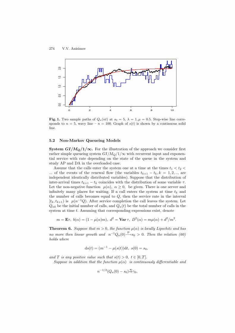
Consider as an illustration of AP a simulation of the system MQ/MQ/1/∞ withthe rates: λ(s) ≡ λ, μ(s) = μs. This case corresponds to a system M/M/∞ andequation (57) implies: s(t) = λ/μ + (s0 − λ/μ)e−μt, t ≥ 0.

Figure 1 illustrates the convergence of the trajectory Qn(nt)/n to the functions(t) for two values of n, n = 5 and n = 100. At large n, the trajectory is closeto s(·).

274 V.V. Anisimov

0 2 4 6 8 10

0.00.5

1.01.5

2.0

Fig. 1. Two sample paths of Qn(nt) at s0 = 5, λ = 1, μ = 0.5. Step-wise line corre-sponds to n = 5, wavy line – n = 100. Graph of s(t) is shown by a continuous solidline.

5.2 Non-Markov Queueing Models

System GI/MQ/1/∞. For the illustration of the approach we consider firstrather simple queueing system GI/MQ/1/∞ with recurrent input and exponen-tial service with rate depending on the state of the queue in the system andstudy AP and DA in the overloaded case.

Assume that the calls enter the system one at a time at the times t1 < t2 <... of the events of the renewal flow (the variables tk+1 − tk, k = 1, 2, .., areindependent identically distributed variables). Suppose that the distribution ofinter-arrival times tk+1 − tk coincides with the distribution of some variable τ .Let the non-negative function μ(α), α ≥ 0, be given. There is one server andinfinitely many places for waiting. If a call enters the system at time tk andthe number of calls becomes equal to Q, then the service rate in the interval[tk, tk+1) is μ(n−1Q). After service completion the call leaves the system. LetQn0 be the initial number of calls, and Qn(t) be the total number of calls in thesystem at time t. Assuming that corresponding expressions exist, denote

m = Eτ, b(α) = (1 − μ(α)m), d2 = Var τ, D2(α) = mμ(α) + d2/m2.

Theorem 6. Suppose that m > 0, the function μ(α) is locally Lipschitz and hasno more then linear growth and n−1Qn(0) P−→s0 > 0. Then the relation (60)holds where

ds(t) = (m−1 − μ(s(t))dt, s(0) = s0,

and T is any positive value such that s(t) > 0, t ∈ [0, T ].Suppose in addition that the function μ(α) is continuously differentiable and

n−1/2(Qn(0) − s0)w⇒γ0.

Switching Queueing Networks 275

Then the sequence of processes γn(t) = n−1/2(Qn(nt) − ns(t)) J-converges inthe interval [0, T ] to the diffusion process γ(t): γ(0) = γ0,

dγ(t) = −μ′(s(t))γ(t)dt +√

μ(s(t)) + d2/m3 dw(t).

Semi-Markov system SM/MSM,Q/1/∞. Consider more general overloadedqueueing system with semi-Markov input and Markov-type service where the ser-vice rate depends on the state of the system and the state of some SMP. Letx(t), t ≥ 0, be a SMP with values in X which stands for some external randomenvironment. Denote by τ(x) a sojourn time in the state x. Let the non-negativefunction μ(x, α), x ∈ X, α ≥ 0, be given. There is one server and infinitelymany places for waiting. Assume that the calls enter the system one at a time atthe times t1 < t2 < ... of the jumps of the process x(t). Denote xk = x(tk +0). Ifa call enters the system at time tk and the number of calls in the system becomesequal to Q, then the service rate in the interval [tk, tk+1) is μ(xk, n−1Q). Afterservice completion the call leaves the system. Let Qn0 be the initial number ofcalls, and Qn(t) be the total number of calls in the system at time t.

Consider the case when the embedded MP xk, k ≥ 0, does not depend onparameter n and is uniformly ergodic with stationary measure π(A), A ∈ BX .Assuming that corresponding expressions exist, denote

m(x) = Eτ(x), m =∫

X

m(x)π(dx), c(α) =∫

X

μ(x, α)m(x)π(dx),

b(α) = (1 − c(α))m−1, G(α) = c′(α),g(x, α) = 1 − m(x)(1 − c(α) + μ(x, α)m)m−1,

d2(x) = Var τ(x), d2 =∫

X

d2(x)π(dx),

e1(α) =∫

X

μ2(x, α)d2(x)π(dx), e2(α) =∫

X

μ(x, α)d2(x)π(dx),

D2(α) = c(α) + e1(α) + 2(1 − c(α))e2(α)m−1 + (1 − c(α))2d2m−2.

Theorem 7. Suppose that m > 0, the function μ(x, α) is locally Lipschitz withrespect to α uniformly in x ∈ X, the function c(α) has no more then lineargrowth and n−1Qn(0) P−→s0 > 0. Then the relation (60) holds where

ds(t) = m−1(1 − c(s(t))dt, s(0) = s0,

and T is any positive value such that s(t) > 0, t ∈ [0, T ].Suppose in addition that variables τ(x)2 are uniformly integrable, the function

c(α) is continuously differentiable, and n−1/2(Qn(0) − s0)w⇒γ0.

Then the sequence of processes γn(t) = n−1/2(Qn(nt) − ns(t)) J-convergesin the interval [0, T ] to the diffusion process γ(t): γ(0) = γ0,

dγ(t) = −m−1G(s(t))γ(t)dt + m−1/2 (D2(s(t)) + B2(s(t)))1/2dw(t),

276 V.V. Anisimov

where

B2(a) = E(g(x0, α)2 + 2

∞∑k=1

g(x0, α)g(xk, α)),

and P{x0 ∈ A} = π(A), A ∈ BX .

Similar results can be proved for the system MSM,Q/MSM,Q/1/∞ where theinput and service rates depend on the state of some external SMP and the valueof the queue, for the system SMQ/MSM,Q/1/∞ where an input forms someprocess of a semi-Markov type with occupation times depending on the valueof the queue, some systems with unreliable servers, polling systems and retrialmodels. More examples can be found in the author’s book [20].

6 Queueing Networks

6.1 Markov Networks

Consider a state-dependent queueing network (MQ/MQ/1/∞)r consisting of rnodes with one server in each node and infinitely many places for waiting. Denoteby Qn(i, t) the number of calls in the i-th node at time t and let Qn(t) =(Qn(i, t), i = 1, r) be the column vector.

We assume that the time goes to infinity in the scale nt and consider the APand DA for the normalized vector-valued queueing process Qn(nt). Let the func-tions {λi(q), μi(q), pij(q), i = 1, r, j = 0, r, q ∈ [0,∞)r} be given. The networkis operating in the following way. If at some time-point u, Qn(u) = Q, then thelocal input rate in the i-th node is λi(Q/n) and the local service rate is μi(Q/n).If at this time a call has completed service in node i, then either with probabilitypij(Q/n) it goes from i-th to j-th node, j = 1, r or with probability pi0(Q/n) itleaves the network. This network belongs to Jackson’s type networks.

Let λ(q) = (λ1(q), ..., λr(q)), μ(q) = (μ1(q), ..., μr(q)) be the column vector-valued functions,

P (q) = ||pij(q)||i,j=1,r , a(q) =r∑

i=1

(λi(q) + μi(q)),

and for a vector-valued function f(q) = (f1(q), ...fr(q)) with q = (q1, ..., qr) wedenote by f ′(q) the matrix derivative: f ′(q) = ||∂fi(q)/∂qj ||i,j=1,r.

Theorem 8. Assume that as n → ∞,

n−1Qn(0) P−→s0, (63)

the functions λ(q), μ(q), P (q), satisfy a local Lipschitz condition, and for somefixed T > 0 there exists A > 0 such that the system of differential equations

dη(t) = (λ(η(t) + (P ∗(η(t)) − I)μ(η(t)))a(η(t))−1dt, η(0) = s0,

Switching Queueing Networks 277

has a unique solution η(t) such that η(t) > 0 in each component, t ∈ (0, A), and∫ A

0 a(η(t))−1dt > T.Then

sup0≤t≤T

|n−1Qn(nt) − s(t)| P−→0, (64)

where the vector-valued function s(t) satisfies the equation:

ds(t) = (λ(s(t)) + (P ∗(s(t)) − I)μ(s(t)))dt, s(0) = s0. (65)

If in additionn−1/2(Qn(0) − ns0)

w⇒γ0, (66)

and the functions λ(q), μ(q), P (q) are continuously differentiable, then the se-quence of processes γn(t) = n−1/2(Qn(nt) − ns(t)) J-converges in the inter-val [0, T ] to a multidimensional diffusion process γ(t) satisfying the followingstochastic differential equation

dγ(t) = G(s(t))γ(t)dt + B(s(t))dω(t), γ(0) = γ0. (67)

Here

G(q) = (λ(q) + ((P ∗(q) − I)μ(q))′, B(q)2 = ||bij(q)||i,j=1,r ,

bij(q) = −μi(q)pij(q) − μj(q)pji(q), i �= j,

bii(q) = −2μi(q)pii(q) + λi(q) + μi(q) +∑

k

μk(q)pki(q), i = 1, r,

and P ∗ is a transposed matrix.

6.2 Non-Markov Queueing Networks

Consider now fluid limit (AP) and DA for some classes of non-Markov networks.The method of analysis is based on the representation of a queueing processas a corresponding SP by choosing in the appropriate way switching times andconstructing corresponding processes in switching intervals.

Network (MSM,Q/MSM,Q/1/∞)r with semi-Markov switching. Sup-pose that characteristics of the network depend on parameter n in the followingway. A SMP x(t) and other variables introduced below do not depend on n.But if at the time t, x(t) = x and Qn(t)/n = q, then the local arrival and ser-vice rates and transition probabilities as well as random sizes of batches η(x, q),κi(x, q) depend on the pair (x, q). Denote by t1 < t2 < ... the times of se-quential jumps of x(t). Suppose that the imbedded MP xk = x(tk), k ≥ 0,

is ergodic with stationary distribution πx, x ∈ X = {1, 2, .., d}. Let Q(i)n (t)

be the size of the queue in node i at time t, and Qn0 be the initial value.

278 V.V. Anisimov

Denote Qn(t) = (Q(1)n (t), ..., Q(r)

n (t)), t ≥ 0, and for any x ∈ X, i = 1, r, q ∈ Rr,introduce the following variables:

m(x) = Eτ(x), P0(x, q) = ||pij(x, q)||i,j=1,r , a(x, q) = Eη(x, q),gi(x, q) = Eκi(x, q), g(x, q) = (μ1(x, q)g1(x, q), .., μr(x, q)gr(x, q)),

m =∑x∈X

m(x)πx, c(x, q) = λ(x, q)a(x, q) + (P0(x, q)∗ − I)g(x, q),

b(q) =∑x∈X

m(x)c(x, q)πx, d2(x) = Var τ(x), d2i (x, q) = Eκ2

i (x, q),

J2(x, q) = λ(x, q)Eη(x, q)η(x, q)∗.

Let F 2(x, q) = ||fij(x, q)||i,j=1,r be the matrix with the following entries:

fij(x, q) = −μi(x, q)pij(x, q)d2i (x, q) − μj(x, q)pji(x, q)d2

j (x, q), i, j = 1, r, i �= j;

fii(x, q) = μi(x, q)(1 − 2pii(x, q))d2i (x, q) +

r∑k=1

μk(x, q)pki(x, q)d2k(x, q).

Denote

D2(x, q) = d2(x)(c(x, q) − m−1b(q)

)(c(x, q) − m−1b(q)

)∗

+ m(x)(F 2(x, q) + J2(x, q)

),

D2(q) =∑x∈X

D2(x, q)πx, (68)

γ(x, q) = m(x)(c(x, q) − m−1b(q)).

Let the matrix B2(q) be calculated using the variables γ(x, q) with the help ofMP xk according to (52), (53) in Theorem 4. We put H2(q) = D2(q) + B2(q).Define H(q) according to the relation H(q)H(q)∗ = H2(q). Let s(t) be a solutionof the equation

ds(t) = m−1b(s(t))dt, s(0) = s0. (69)

Theorem 9. 1) Assume that the functions λ(x, q), μi(x, q), a(x, q), gi(x, q),pij(x, q) for any x ∈ X, i = 1, r, j = 1, r + 1, are locally Lipschitz with re-spect to q ∈ int{Rm

+}, and Eτ(x)2 < ∞, x ∈ X. Let also m > 0, for anybounded and closed domain G ∈ int{Rm

+},

Eκi(x, q)2 ≤ CG, E|η(x, q)|2 ≤ CG, i = 1, r, x ∈ X, q ∈ G, (70)

where CG < ∞, the function b(q) has no more than linear growth, n−1Qn(0) P−→s0 > 0, and there exists T > 0 such that s(t) > 0, t ∈ [0, T ], in each component.

Thensup

0≤t≤T|n−1Qn(nt) − s(t)| P−→ 0. (71)

Switching Queueing Networks 279

2) Assume in addition that there exists a continuous matrix derivative G(q) =b ′(q), q ∈ int{Rm

+}, Eτ(x)3 < ∞, x ∈ X, and for any bounded and closeddomain G ∈ int{Rm

+},

Eκi(x, q)3 ≤ CG, E|η(x, q)|3 ≤ CG, i = 1, r, x ∈ X, q ∈ G. (72)

Let alson−1/2(Qn(0) − ns(0)) w⇒ γ0, (73)

and the function H2(q) is continuous.Then the sequence γn(t) = n−1/2(Qn(nt)− ns(t)) J-converges in Dr

T to thediffusion process γ(t):

dγ(t) = G(s(t))γ(t)dt + m−1/2H(s(t))dw(t), γ(0) = γ0. (74)

The proof is given in the book [20].

7 Aggregation in Markov Models with Fast Switching

In this section we consider the approximation of Markov type queueing modelswith fast Markov switching by Markov models with averaged transition rates.Consider first some general setting. Let (xn(t), ζn(t)) be a two-component MP.The following result is proved in [18,20].

Assume that a component xn(·) has fast switching and satisfy the asymptoticmixing condition. Assume also that the transition rates of ζn(t) depend on thecomponent xn(·) and the process ζn(t) has rather slow transitions, that means,the number of transitions in any finite interval is bounded in probability.

Then under rather general conditions the component ζn(·) J-converges in Sko-rokhod space to a MP with transition rates averaged by some quasi-stationarymeasures constructed by xn(·). The convergence of a stationary distribution of(xn(·), ζn(·)) is studied as well.

Example 1: ζn(t) is a MP with local rates λ(i, j, xn(t)), where xn(t) is a fastMarkov environment.

Example 2: ζn(t) is a quasi-Birth-and-Death process, that has fast transitionsin each level and slow transitions between levels.

Consider now as an example an approximation of a queueing model with fastMarkov switching by a simpler queueing model with averaged transition rates.

7.1 System MM,Q/MM,Q/1/N with Fast Markov Switching

Consider a queueing system in a fast Markov environment. A system consistsof one server and N waiting places. Assume that the calls arrive according toa state-dependent Poisson process with Markov switching and also at the timesof jumps of a switching MP. If the system is full, an arriving call is lost. Letx0(t), t ≥ 0, be an ergodic MP with values in X = {x1, ..., xr}. Denote byρ(x), x ∈ X, its stationary distribution. Let b(x) be the exit rate from state

280 V.V. Anisimov

x, x ∈ X . We define a Markov environment with fast switching as follows: xn(t) =x0(Vnt), t ≥ 0, where Vn is some scaling factor, Vn → ∞.

Denote by ϕ0(·) and ϕn(·) uniformly strong mixing coefficients for processesx0(·) and xn(·), respectively. According to ergodicity of x0(·), there exist q < 1and L > 0 such that ϕ0(L) ≤ q. Then ϕn(L/Vn) = ϕ0(L) ≤ q, and thereforexn(·) is asymptotically mixing in any fixed interval.

Let {λ(x, i), μ(x, i), αA(x, i), αS(x, i), x ∈ X, i ≥ 0} be the non-negativefunctions. Denote by Qn(t)), t ≥ 0, the total number of calls in the systemat time t. The system is switched by the process (xn(t), Qn(t)) as follows:if (xn(t), Qn(t)) = (x, i), then the local arrival rate is λ(x, i), and the lo-cal service rate is μ(x, i). Moreover, if at the time tnk of k-th jump of xn(t),(xn(tnk − 0), Qn(tnk − 0)) = (x, i), then either an additional call may enterthe system with probability V −1

n αA(x, i), or a call on service may complete ser-vice with probability V −1

n αS(x, i) (no changes in the system with probability1 − V −1

n (αA(x, i) + αS(x, i)). Put

λ(i) =∑x∈X

λ(x, i)ρ(x), μ(i) =∑x∈X

μ(x, i)ρ(x),

αA(i) =∑x∈X

αA(x, i)b(x)ρ(x), αS(i) =∑x∈X

αS(x, i)b(x)ρ(x), (75)

A(i) = λ(i) + αA(i), Γ (i) = μ(i) + αS(i), i = 0, .., N + 1,

where we set Γ (0) = 0, A(N + 1) = 0. Let MQ/MQ/1/N be an averagedstate-dependent queueing system (system with averaged rates and probabilities)operating as follows: as Q(t) = i, the arrival rate is A(i) and the service rate isΓ (i), where Q(t) is a number of calls in the system at time t.

Theorem 10. If MP Q(·) is regular and Qn(0) = q0, then for any N ≤ ∞,Qn(·) J-converges in each finite interval [0, T ] to Q(·), where Q(0) = q0.

The approximation of a stationary distribution can be proved as well. Denoteby ρn(x, i), x ∈ X, i = 0, .., N + 1, the stationary distribution (if it exists) of theprocess (xn(t), Qn(t)). Assume that N < ∞ and keep notation (75).

Theorem 11. Suppose that A(i) > 0, Γ (i) > 0, λ(x, i)+μ(x, i) > 0, x ∈ X, i =0, .., N + 1. Then Q(·) is ergodic, ρn(x, i) exists at large n and as n → ∞,

ρn(x, i) → ρ(x)Π(i), x ∈ X, i = 0, .., N + 1,

where Π(i), i = 0, .., N + 1, is the stationary distribution of Q(·).Similar result holds when N = ∞.

Analogous results can be proved for batch systems BMM,Q/BMM,Q/1/N ,priority models, models with unreliable servers with slow failures/repairs, modelswith fast semi-Markov switching [18,20].

Another interesting direction of the investigation of transient phenomena isthe class of so-called retrial queues and queues with negative arrivals. Someresults in this direction are obtained in [12,14,16,20].

Switching Queueing Networks 281

7.2 Aggregation in Heavy Traffic Conditions

A new direction of the investigation is the class of queueing models in heavy traf-fic conditions with fast switching, where the switching component itself allowsan asymptotic aggregation of states. A more formal setting is the following. Con-sider a switching queueing model which is described by a two component process(xn(t), Qn(t)), where xn(t) is a MP with state space satisfying the conditions ofthe asymptotic aggregation of state space [1,3,4] (see also [20]). This means thatthe state space can be subdivided on the aggregated regions: fast transitionswithin each region and slow transitions between regions. The transition rates ofthe queueing process Qn(t) may depend on the states of (xn(t), Qn(t)). Assumealso that for the process Qn(t) the number of transitions in any finite interval isgoing in probability to infinity and the values of Qn(t) are also asymptoticallyunbounded, e.g. Qn(t) is the queue in heavy traffic conditions.

Basing on the results of Section 5 we can see that in the case when thecomponent xn(t) satisfies an asymptotic mixing condition, an AP and DA typetheorems for Qn(t) hold. However, in this case the process xn(t) satisfy the con-ditions of the asymptotic aggregation of states and does not satisfies asymptoticmixing conditions.

Thus, we can expect that under rather general conditions the process xn(t)weakly converges to y(t), where xn(t) is an aggregated process (the state space isthe space of regions) and y(t) is a MP with averaged transition rates [1,3,4,20].Correspondingly, under heavy-traffic conditions, the process Qn(t)/n in eachregion converges to a solution of differential equation.

Therefore, the two-component process (xn(t), Qn(t)/n) should converge toa MP (y(t), Q0(t)), where Q0(t) satisfied a differential equation with Markovswitching of the form dQ0(t) = A(y(t), Q0(t))dt, and A(i, q) are the aggregatedrates in each region. The results of this type are still not fully investigated. Someresults in this direction are published in [13,33].

8 Conclusions

The asymptotic results described in Sections 4-6 allow to approximate the be-haviour of queueing processes for rather complicated switching queueing systemsand networks under heavy traffic conditions by much simpler processes, in par-ticular, by solutions of differential equations or by diffusion processes. Section 7deals with the approximation of complex queueing models by simpler ones withthe rates averaged by some stationary measures.

These results are also valid for the approximation of various functionals de-fined on the trajectory of the queuing process, e.g., the cumulative reward orlosses, time to reach a critical region, time spend by a queueing process in agiven region, different stationary characteristics, etc. In particular, various per-formance measures of operating of complex queueing models can be approxi-mated by corresponding measures of much simpler processes.

Therefore, these results provide us with the new analytic technique for theperformance evaluation of complex queueing systems and networks.

282 V.V. Anisimov

Acknowledgments. The author is thankful to Professor Demetres Kouvatsosfor a long term fruitful collaboration.

References

1. Anisimov, V.V.: Asymptotic Consolidation of the States of Random Processes.Cybernetics 9(3), 494–504 (1973)

2. Anisimov, V.V.: Switching Processes. Cybernetics 13(4), 590–595 (1977)3. Anisimov, V.V.: Limit Theorems for Switching Processes and their Applications.

Cybernetics 14(6), 917–929 (1978)4. Anisimov, V.V.: Random Processes with Discrete Component. Limit Theorems.

Publ. Kiev Univ. (1988) (Russian)5. Anisimov, V.V.: Limit Theorems for Switching Processes. Theory Probab. and

Math. Statist. 37, 1–5 (1988)6. Anisimov, V.V., Aliev, A.O.: Limit Theorems for Recurrent Processes of Semi-

Markov Type. Theory Probab. and Math. Statist. 41, 7–13 (1990)7. Anisimov, V.V.: Averaging Principle for Switching Processes. Theory Probab. and

Math. Statist. 46, 1–10 (1992)8. Anisimov, V.V.: Averaging Principle for the Processes with Fast Switching.

Random Oper. & Stoch. Eqv. 1(2), 151–160 (1993)9. Anisimov, V.V.: Limit Theorems for Processes with Semi-Markov Switching and

their Applications. Random Oper. & Stoch. Eqv. 2(4), 333–352 (1994)10. Anisimov, V.V.: Switching Processes: Averaging Principle, Diffusion Approxima-

tion and Applications. Acta Applicandae Mathematicae 40, 95–141 (1995)11. Anisimov, V.V.: Asymptotic Analysis of Switching Queueing Systems in Condi-

tions of Low and Heavy Loading. In: Alfa, A.S., Chakravarthy, S.R. (eds.) Matrix-Analytic Methods in Stochastic Models. Lect. Notes in Pure and Appl. Mathem.Series, vol. 183, pp. 241–260. Marcel Dekker, Inc., New York (1996)

12. Anisimov, V.V.: Averaging Methods for Transient Regimes in Overloading RetrialQueuing Systems. Mathematical and Computing Modelling 30(3/4), 65–78 (1999)

13. Anisimov, V.V.: Diffusion Approximation for Processes with Semi-Markov Switchesand Applications in Queueing Models. In: Janssen, J., Limnios, N. (eds.) Semi-Markov Models and Applications, pp. 77–101. Kluwer Academic Publishers, Dor-drecht (1999)

14. Anisimov, V.V.: Switching Stochastic Models and Applications in Retrial Queues.Top 7(2), 169–186 (1999)

15. Anisimov, V.V.: Asymptotic Analysis of Reliability for Switching Systems inLight and Heavy Traffic Conditions. In: Limnios, N., Nikulin, M. (eds.) RecentAdvances in Reliability Theory: Methodology, Practice and Inference, pp. 119–133. Birkhauser, Boston (2000)

16. Anisimov, V.V., Artalejo, J.R.: Analysis of Markov Multiserver Retrial Queueswith Negative Arrivals. Queueing Systems 39(2/3), 157–182 (2001)

17. Anisimov, V.V.: Diffusion Approximation in Overloaded Switching QueueingModels. Queueing Systems 40(2), 141–180 (2002)

18. Anisimov, V.V.: Averaging in Markov Models with Fast Markov Switches andApplications to Queueing Models. Annals of Operations Research 112(1), 63–82(2002)

19. Anisimov, V.V.: Averaging in Markov Models with Fast Semi-Markov Switches andApplications. Communications in Statistics - Theory and Methods 33(3), 517–531(2004)

Switching Queueing Networks 283

20. Anisimov, V.V.: Switching Processes in Queueing Models. Wiley & Sons, ISTE,London (2008)

21. Anisimov, V.V., Zakusilo, O.K., Dontchenko, V.S.: The Elements of QueueingTheory and Asymptotic Analysis of Systems. Publ. ”Visca Scola”, Kiev (1987)(in Russian)

22. Anisimov, V.V., Lebedev, E.A.: Stochastic Queueing Networks. Markov Models.Kiev Univ., Kiev (1992) (in Russian)

23. Buslenko, N.P., Kalashnikov, V.V., Kovalenko, I.N.: Lectures on the Theory ofComplex Systems. Sov. Radio, Moscow (1973) (in Russian)

24. Ezov, I.I., Skorokhod, A.V.: Markov Processes which are Homogeneous in theSecond Component. Theor. Probab. Appl. 14, 679–692 (1969)

25. Ethier, S.N., Kurtz, T.G.: Markov Processes, Characterization and Convergence.J. Wiley & Sons, New York (1986)

26. Gikhman, I.I., Skorokhod, A.V.: Theory of Random Processes, vol. II. Springer,Heidelberg (1975)

27. Griego, R., Hersh, R.: Random Evolutions, Markov Chains, and Systems of PartialDifferential Equations. Proc. Nat. Acad. Sci. 62, 305–308 (1969)

28. Hersh, R.: Random Evolutions: Survey of Results and Problems. Rocky Mount. J.Math. 4(3), 443–475 (1974)

29. Korolyuk, V.S., Swishchuk, A.V.: Random Evolutions. Kluwer Acad. Publ.,Dordrecht (1994)

30. Korolyuk, V.S., Korolyuk, V.V.: Stochastic Models of Systems. Kluwer, Dordrecht(1999)

31. Korolyuk, V.S., Limnios, N.: Evolutionary Systems in an Asymptotic Split StateSpace. In: Limnios, N., Nikulin, M. (eds.) Recent Advances in Reliability Theory:Methodology, Practice and Inference, pp. 145–161. Birkhauser, Boston (2000)

32. Korolyuk, V.S., Limnios, N.: Average and Diffusion Approximation for Evolution-ary Systems in an Asymptotic Split Phase State. Ann. Appl. Prob. 14(1), 489–516(2004)

33. Korolyuk, V.S., Limnios, N.: Stochastic Systems in Merging Phase Space. WorldScientific, Singapore (2005)

34. Korolyuk, V.S., Korolyuk, V.V., Limnios, N.: Queueing Systems with Semi-MarkovFlow in Average and Diffusion Approximation Schemes. Methodol. Comput. Appl.Probab. 11, 201–209 (2009)

35. Neuts, M.: Structured Stochastic Matrices of M/G/1 Type and Their Applications.Marcel Dekker, New York (1989)

36. Skorokhod, A.V.: Limit Theorems for Random Processes. Theory Probab. Appl. 1,289–319 (1956)