Neural Networks 36 (2012) 136–145

Contents lists available at SciVerse ScienceDirect

Neural Networks

journal homepage: www.elsevier.com/locate/neunet

Global exponential estimates of delayed stochastic neural networks withMarkovian switchingHe Huang a,∗, Tingwen Huang b, Xiaoping Chen a

a School of Electronics and Information Engineering, Soochow University, Suzhou 215006, PR Chinab Texas A & M University at Qatar, Doha 5825, Qatar

a r t i c l e i n f o

Article history:Received 18 April 2012Received in revised form 30 August 2012Accepted 7 October 2012

Keywords:Stochastic neural networksMarkovian switchingExponential estimatesTime delayMode-dependent

a b s t r a c t

This paper is concerned with the global exponential estimating problem of delayed stochastic neuralnetworks with Markovian switching. By fully taking the inherent characteristic of such kinds of neuralnetworks into account, a novel stochastic Lyapunov functional is constructed in which as many aspossible of the positive definite matrices are dependent on the system mode and a triple-integral termis introduced. Based on it, a delay- and mode-dependent criterion is derived under which not only theneural network is mean square exponentially stable but also the decay rate is well obtained. Moreover,it is shown that the established stability condition includes some existing ones as its special cases, and isthus less conservative. This approach is then extended to twomore general cases wheremode-dependenttime-varying delays and parameter uncertainties are considered. Finally, three numerical examples arepresented to demonstrate the performance and effectiveness of the developed approach.

© 2012 Elsevier Ltd. All rights reserved.

1. Introduction

During the past few years, various kinds of recurrent neuralnetworks have been proposed including bidirectional associa-tive memory neural networks, cellular neural networks, Co-hen–Grossberg neural networks andHopfield neural networks, etc.Many exciting applications have been established in knowledge ac-quisition, combinatorial optimization, adaptive control, signal pro-cessing, prediction and other areas (Haykin, 1999). Generally, aprerequisite to these successful applications is the stability of theunderlying neural networks. As a result, much effort has been de-voted to the stability analysis of recurrent neural networks.

In electronic implementations of neural networks, time delaysare frequently inevitable in the process of information storageand transmission. A main disadvantage of the presence of timedelays is to lead to instability and oscillation. On the other hand,it has been recognized that better performance can be achievedwhen time delays are intentionally introduced for some specialcircumstances (Roska & Chua, 1992) (e.g., speed detection ofmoving objects and processing of moving images). Consequently,the study of recurrent neural networks with time delays hasgained a great deal of attention. Many interesting results relatedto the stability analysis have been reported in the literature

∗ Corresponding author. Tel.: +86 512 67871211; fax: +86 512 67871211.E-mail addresses: cshhuang@gmail.com, hhuang@suda.edu.cn (H. Huang),

tingwen.huang@qatar.tamu.edu (T. Huang), xpchen@suda.edu.cn (X. Chen).

0893-6080/$ – see front matter© 2012 Elsevier Ltd. All rights reserved.doi:10.1016/j.neunet.2012.10.002

(Faydasicok & Arik, 2012; Li, Gao, & Yu, 2011; Liu, Chen, Cao, &Lu, 2011; Marco, Grazzini, & Pancioni, 2011; Wu, Liu, Shi, He, &Yokoyama, 2008; Zeng & Wang, 2006; Zhang & Han, 2009; Zhang,Liu, Huang, & Wang, 2010; Zheng, Zhang, & Wang, 2011).

In real nervous systems, the synaptic transmission can beregarded as a noisy process because of random fluctuations fromthe release of neurotransmitters and other probabilistic causes.As observed in Blythe, Mao, and Shah (2001) and Liao and Mao(1996); Shen andWang (2007), a neural network can be stabilizedor destabilized by certain stochastic inputs. It motivates the studyof the stability analysis problemof stochastic neural networks (see,for examples, Chen & Zheng, 2010, Wang, Liu, Li, & Liu, 2006, Yang,Gao, & Shi, 2009, Zhang, Xu, Zong, & Zou, 2009 and the referencestherein).

Furthermore, in practice, the phenomenonof information latch-ing often appears in neural networks. Fortunately, it can be ef-ficiently tackled by extracting a finite state representation fromthe network (Tino, Cernansky, & Benuskova, 2004; Wu, Shi, Su,& Chu, 2011). That is to say, the neural networks with informa-tion latching may have finite modes which can switch from oneto another at different times. It has been known (Zhang & Wang,2008; Zhu & Cao, 2011) that the Markov chain provides one ofthe promisedways to characterize the switching between differentmodes. Therefore, the study of delayed stochastic neural networkswithMarkovian switching is of great significance and practical im-portance, and plays an essential role to the potential applicationsin the field of information science. Recently, many methods (forexamples, the delay partitioning technique and the free-weighting

H. Huang et al. / Neural Networks 36 (2012) 136–145 137

matrices based method) have been adopted to deal with this issue(Balasubramaniam & Lakshmanan, 2009; Huang, Ho, & Qu, 2007;Liu, Ou, Hu, & Liu, 2010; Liu, Wang, Liang, & Liu, 2009; Liu, Wang, &Liu, 2008; Lou&Cui, 2007;Ma, Xu, Zou, & Lu, 2011;Wang, Liu, Yu, &Liu, 2006;Wu, Shi, Su, & Chu, 2012; Yang, Cao, & Lu, 2012; Zhang &Wang, 2008; Zhu & Cao, 2010, 2011). InWang, Liu, Yu et al. (2006),the authors discussed the exponential stability analysis problem ofrecurrent neural networks with time delays and Markovian jump-ing parameters. A delay-independent condition was obtained bymeans of linear matrix inequalities (LMIs) (Boyd, El Ghaoui, Feron,& Balakrishnan, 1994). At the same time, the authors in Huanget al. (2007) studied the global robust stability of stochastic ad-ditive neural networks with Markovian switching and intervaluncertainties. In Ma et al. (2011), a delay-dependent stability con-dition was derived for uncertain stochastic neural networks withMarkovian jumping parameters and mixed mode-dependent de-lays by introducing some slack matrices (or free-weighting matri-ces). In Liu et al. (2010), the authors studied the stability analysisproblem of delayed bidirectional associative memory neural net-workswithMarkovian jumping parameters by using the delay par-titioning approach. However, it should be noted that, inmost of theabove results, only a part of the positive definite matrices (i.e., thematrices involved in the quadratic form and the single-integralterms of the constructed stochastic Lyapunov functionals) are de-pendent on the system mode, while the matrices in the double-integral terms are common for all modes. It is thus expected thatless conservative stability criteria could be established ifmore pos-itive definite matrices are chosen to be mode-dependent. This isbecause the choice of the positive definite matrices in the lattercase obviously has more freedom than that in the former case. Inaddition, as suggested in Shu and Lam (2008), the transient processof a neural network can be clearly characterized once its decay rateis explicitly known. Therefore, the exponential stability analysis isalso of practical value. These motivate the present study.

In this paper, our attention focuses on the global exponential es-timating problem of a class of delayed stochastic neural networkswithMarkovian switching. By fully considering its inherent charac-teristic, a new stochastic Lyapunov functional is constructed withas many as possible mode-dependent positive definite matricesand an additional tripe-integral term. The role of this triple-integralterm is such that some positive definite matrices in the double-integral terms, which are common in the above literature, dependon the system mode. Then, a delay- and mode-dependent stabil-ity condition is established in terms of LMIs. It should be pointedout that the obtained LMIs are monotonically increasing with re-spect to the decay rate. Therefore, the upper bound of the decayrate can be efficiently found by solving a corresponding convex op-timization problem, which is facilitated readily by some availablealgorithms (e.g., the interior point algorithm) (Boyd et al., 1994).It is further shown from a point of view of theory that the stabil-ity criterion includes some previous ones as its special cases and isthus less conservative. Themain contributions of this study are that(i) a novel stability condition is derived; (ii) the upper bound of thedecay rate can be easily obtained; and (iii) the less conservatism ofour approach is rigorously proven. Moreover, this approach is thenextended to address the global exponential estimating problemof stochastic neural networks with Markovian switching, mode-dependent time-varying delays and parameter uncertainties. Fi-nally, several examples are provided to illustrate the performanceand effectiveness of the developed approach.

Notation: The following notations will be used throughout thispaper. Let R denote the set of real numbers, R+ the set of non-negative real numbers, Rn the n-dimensional Euclidean space andRn×m the set of all n × m real matrices. The superscript ‘‘T ’’represents the transpose. I is the identity matrix with appropri-ate dimension. The symbol ∗ denotes the symmetric block in a

symmetric matrix. For any real square matrices X and Y , X >

Y (X ≥ Y , X < Y , X ≤ Y ) means that X–Y is symmetric andpositive definite (positive semi-definite, negative definite, nega-tive semi-definite, respectively), and X > 0 (X ≥ 0, X < 0, X≤ 0) means that X is symmetric and positive definite (positivesemi-definite, negative definite, negative semi-definite, respec-tively); Tr(X) is the trace of X; λmax(X) and λmin(X) are respec-tively the maximum and minimum eigenvalues of X . For τ >

0, C ([−τ , 0]; Rn) denotes the family of continuous functions ϕ

from [−τ , 0] to Rn with the norm ∥ϕ∥ = sup−τ≤ϑ≤0 |ϕ(ϑ)|,where | · | is the Euclidean norm in Rn. Let (Ω, F , P) be a com-plete probability spacewith a filtration Ftt≥0 satisfying the usualconditions (i.e. it is right continuous and F0 contains all P-pullsets); C b

F0([−τ , 0]; Rn) the family of all bounded, F0-measurable,

C ([−τ , 0]; Rn)-valued random variables; C 2,1(Rn× R+

× S; R+)

the family of all nonnegative functions V (u, t, i) on Rn× R+

× Swhich are continuously twice differentiable in u and differentiablein t . Themathematical expectation operatorwith respect to a givenprobability measure P is denoted by E.

2. Problem formulation

Similar to (Huang et al., 2007; Wang, Liu, Yu et al., 2006; Zhu &Cao, 2011), the delayed stochastic neural network with Markovianswitching considered in this paper is described by

du(t) = [−E(r(t))u(t) + A(r(t))f (u(t))+ C(r(t))h(u(t − τ(t)))]dt+ σ(u(t), u(t − τ(t)), t, r(t))dw(t) (1)

u(t) = ξ(t), t ∈ [−τ , 0], r(0) = r0, (2)

where u(t) = [u1(t), u2(t), . . . , un(t)]T is the state vector asso-ciated with n neurons, w(t) is a m-dimensional Browian motionon the complete probability space (Ω, F , P), r(t)t≥0, which issupposed to be independent of w(t), is a right-continuous Markovchain defined on the complete probability space (Ω, F , P) andtaking values in a finite state space S = 1, 2, . . . ,N with transi-tion probability matrix Q = (qij)N×N given by

Pr(t + ∆) = j|r(t) = i =

qij∆ + o(∆), if i = j1 + qii∆ + o(∆), if i = j

with ∆ > 0 and lim∆→0+ o(∆)/∆ = 0. Here, qij ≥ 0 (i = j) is thetransition rate from i to j, and

qii = −

Nj=1,j=i

qij. (3)

E(r(t)) = diag(e1(r(t)), e2(r(t)), . . . , en(r(t))) is the firing ratematrix with positive entries, A(r(t)) and C(r(t)) are respec-tively the connection weight matrix and the delayed connectionweight matrix, f (u(t)) = [f1(u1(t)), f2(u2(t)), . . . , fn(un(t))]T andh(u(t)) = [h1(u1(t)), h2(u2(t)), . . . , hn(un(t))]T are the activationfunctions, the noise perturbation σ : Rn

×Rn×R+

× S → Rn×m isa Borel measurable function, τ(t) is a time-varying delay with anupper bound τ > 0, ξ(t) ∈ C b

F0([−τ , 0]; Rn) is an initial function

and r0 ∈ S is an initial mode.For the sake of simplicity, for each r(t) = i ∈ S, we denote

E(r(t)) = Ei, A(r(t)) = Ai, C(r(t)) = Ci and σ(u(t), u(t −

τ(t)), t, r(t)) = σ(u(t), u(t − τ(t)), t, i) (or sometimes σ(t, i)).As in Zhu and Cao (2011), the following assumptions are alwaysmade:

138 H. Huang et al. / Neural Networks 36 (2012) 136–145

Assumption 1. The activation functions fj(·) and hj(·) satisfyfj(0) = hj(0) = 0 and

µ−

1j ≤fj(x) − fj(y)

x − y≤ µ+

1j, (4)

µ−

2j ≤hj(x) − hj(y)

x − y≤ µ+

2j (5)

for all x = y ∈ R and j = 1, 2, . . . , n with µ−

1j, µ+

1j, µ−

2j and µ+

2jbeing constant scalars.

Assumption 2. There are two scalars τ and ρ such that

0 ≤ τ(t) ≤ τ and τ (t) ≤ ρ. (6)

Assumption 3. σ(0, 0, t, r(t)) ≡ 0 and there exist real matricesR1i > 0 and R2i > 0 (i = 1, 2, . . . ,N) such that

Tr[σ T (x, y, t, i)σ (x, y, t, i)] ≤ xTR1ix + yTR2iy (7)

for any x, y ∈ Rn and r(t) = i.The objective of this study is to develop a novel approach

to dealing with the global exponential estimating problem ofthe delayed stochastic neural network with Markovian switching(1). The basic idea is to introduce a triple-integral term into thestochastic Lyapunov functional such that as many as possibleof the positive definite matrices are dependent on the systemmode i.

Remark 1. In Zhu and Cao (2011), the following stochastic neuralnetworkwithMarkoivian jump parameters andmixed time delayswas studied

dy(t) =

−E(r(t))y(t) + A(r(t))f (y(t)) + B(r(t))g(y(t − τ1))

+ C(r(t))h(y(t − τ2(t))) + D(r(t))

×

t

t−τ3(t)l(y(s))ds

dt + σ(y(t), y(t − τ1),

y(t − τ2(t)), y(t − τ3(t)), t, r(t))dw(t). (8)

Obviously, (8) is more general than (1). The reason why (1) isinvestigated here is to clearly exhibit the basic idea of the newly-proposed approach. In fact, one can easily extend this approach tohandling the global exponential estimating problem of (8).

To ensure the existence and uniqueness of the solution of (1), allσ(x, y, t, i) (i ∈ S) are additionally assumed to be locally Lipschitzcontinuous and satisfy linear growth condition (Mao, Matasov, &Piunovskiy, 2000). For any initial conditions ξ ∈ C b

F0([−τ , 0]; Rn)

and r0 ∈ S, the unique solution of (1) is denoted by u(t; ξ) (orsometimes simply by u(t)). Moreover, from Assumptions 1 and 3,(1) has a trivial solution u(t; 0) = 0.

Definition 1. The delayed stochastic neural network (1) with (2)is said to be mean square exponentially stable if there exist twoscalars α > 0 and β > 0 such that

E|u(t; ξ)|2 ≤ αe−βtE∥ξ∥2 (9)

holds for any initial conditions ξ ∈ C bF0

([−τ , 0]; Rn) and r0 ∈ S.In this case, the scalars α and β are respectively called the decaycoefficient and decay rate.

Let ut = u(t + ϑ), −τ ≤ ϑ ≤ 0. It is known from Mao(2002) and Skorohod (1989) that ut , r(t)t≥0 is aC ([−τ , 0]; Rn)×

S-valued Markov process. Then, its infinitesimal operator L on afunctional V ∈ C 2,1(Rn

× R+× S; R+) is defined by

L V (ut , t, i) = lim∆→0+

1∆

E(V (ut+∆, t

+ ∆, r(t + ∆))|ut , r(t) = i) − V (ut , t, i).

By the generalized Itô’s formula, one has

EV (ut , t, r(t)) = EV (u(0), 0, r(0)) + E t

0L V (us, s, r(s))ds.

3. Main results

Let

β1 =eβτ

− 1β

, β2 =eβτ

− βτ − 1β2

,

U−

1 = diag(µ−

11, µ−

12, . . . , µ−

1n),

U+

1 = diag(µ+

11, µ+

12, . . . , µ+

1n),

U−

2 = diag(µ−

21, µ−

22, . . . , µ−

2n),

U+

2 = diag(µ+

21, µ+

22, . . . , µ+

2n).

Theorem 1. For given scalars τ > 0, ρ and β > 0, the delayedstochastic neural network (1) with (2) is mean square exponentiallystable with a prescribed decay rate β if there exist real matrices Pi >0, Fi > 0, Li > 0,Mi > 0, X1 > 0, X2 > 0, Ski = diag(sik1,sik2, . . . , s

ikn) > 0 and scalars λi > 0 (i = 1, 2, . . . ,N and k =

1, 2, 3) such that the following LMIs

Pi ≤ λiI, (10)

eβτNj=1

qijFj ≤ X1, (11)

eβτNj=1

qijLj ≤ Mi, (12)

eβτNj=1

qijMj ≤ X2, (13)

Θ =

Θ1 0 Θ2 Θ3 PiCi∗ Θ4 0 0 Θ5∗ ∗ −2S1i 0 0∗ ∗ ∗ Θ6 0∗ ∗ ∗ ∗ Θ7

< 0 (14)

are satisfied for i = 1, 2, . . . ,N, where

Θ1 = βPi − PiEi − ETi Pi +

Nj=1

qijPj + λiR1i + eβτ Fi

+ β1X1 − 2U+

1 S1iU−

1 − 2U+

2 S2iU−

2 ,

Θ2 = PiAi + (U−

1 + U+

1 )S1i, Θ3 = (U−

2 + U+

2 )S2i,

Θ4 = λiR2i − (1 − ρ)Fi − 2U+

2 S3iU−

2 ,

Θ5 = (U−

2 + U+

2 )S3i,

Θ6 = eβτ Li + β1Mi + β2X2 − 2S2i,Θ7 = −(1 − ρ)Li − 2S3i.

Proof. It follows from (7) and (10) that

Tr[σ T (t, i)Piσ(t, i)] ≤ λiTr[σ T (t, i)σ (t, i)]≤ λiuT (t)R1iu(t)

+ λiuT (t − τ(t))R2iu(t − τ(t)). (15)

H. Huang et al. / Neural Networks 36 (2012) 136–145 139

Since 0 ≤ τ(t) ≤ τ , X1 > 0 and (11), one can derive that fori = 1, 2, . . . ,N ,

Nj=1

qij

t

t−τ(t)eβ(s+τ)uT (s)Fju(s)ds

≤

t

t−τ(t)eβsuT (s)X1u(s)ds

≤ eβt t

t−τ

uT (s)X1u(s)ds. (16)

That is, for the positive definite matrices Fj and X1 satisfying (11),the inequality

Nj=1

qij

t

t−τ(t)eβ(s+τ)uT (s)Fju(s)ds

− eβt t

t−τ

uT (s)X1u(s)ds ≤ 0 (17)

is true.Similarly, it can be shown that (12) and (13) respectively

guarantee

Nj=1

qij

t

t−τ(t)eβ(s+τ)hT (u(s))Ljh(u(s))ds

− eβt t

t−τ

hT (u(s))Mih(u(s))ds ≤ 0, (18)

Nj=1

qij

0

−τ

t

t+θ

eβ(s−θ)hT (u(s))Mjh(u(s))dsdθ

− eβt 0

−τ

t

t+θ

hT (u(s))X2h(u(s))dsdθ ≤ 0. (19)

In addition, for anydiagonalmatrices Ski = diag(sik1, sik2, . . . , s

ikn) >

0 (k = 1, 2, 3), it is known from Assumption 1 that

0 ≤ −2eβtn

j=1

si1j[fj(uj(t)) − µ+

1juj(t)][fj(uj(t)) − µ−

1juj(t)]

= eβt−2f T (u(t))S1if (u(t)) + 2f T (u(t))S1iU−

1 u(t)+ 2uT (t)U+

1 S1if (u(t)) − 2uT (t)U+

1 S1iU−

1 u(t), (20)

0 ≤ eβt−2hT (u(t))S2ih(u(t)) + 2hT (u(t))S2iU−

2 u(t)+ 2uT (t)U+

2 S2ih(u(t)) − 2uT (t)U+

2 S2iU−

2 u(t), (21)

0 ≤ eβt−2hT (u(t − τ(t)))S3ih(u(t − τ(t)))

+ 2hT (u(t − τ(t)))S3iU−

2 u(t − τ(t))+ 2uT (t − τ(t))U+

2 S3ih(u(t − τ(t)))− 2uT (t − τ(t))U+

2 S3iU−

2 u(t − τ(t)). (22)

Now, construct a stochastic Lyapunov functional candidate for eachi ∈ S as

V (ut , t, i) =

3k=1

Vk(ut , t, i) (23)

with

V1(ut , t, i) = eβtuT (t)Piu(t),

V2(ut , t, i) =

t

t−τ(t)eβ(s+τ)uT (s)Fiu(s)ds

+

0

−τ

t

t+θ

eβ(s−θ)uT (s)X1u(s)dsdθ,

V3(ut , t, i)

=

t

t−τ(t)eβ(s+τ)hT (u(s))Lih(u(s))ds

+

0

−τ

t

t+θ

eβ(s−θ)hT (u(s))Mih(u(s))dsdθ

+

0

−τ

0

θ

t

t+γ

eβ(s−γ )hT (u(s))X2h(u(s))dsdγ dθ.

By directly computing and employing (15), one has

L V1(ut , t, i) = βeβtuT (t)Piu(t) + 2eβtuT (t)× Pi

−Eiu(t) + Aif (u(t)) + Cih(u(t − τ(t)))

+ eβtTr[σ T (t, i)Piσ(t, i)] + eβt

Nj=1

qijuT (t)Pju(t)

≤ eβt

uT (t)

βPi − PiEi − ET

i Pi

+

Nj=1

qijPj + λiR1i

u(t) + 2uT (t)PiAif (u(t))

+ 2uT (t)PiCih(u(t − τ(t)))

+λiuT (t − τ(t))R2iu(t − τ(t))

. (24)

Taking the infinitesimal operator on V2(ut , t, i) and noting (6) yield

L V2(ut , t, i) ≤ eβ(t+τ)uT (t)Fiu(t)− (1 − ρ)eβtuT (t − τ(t))Fiu(t − τ(t))

+

Nj=1

qij

t

t−τ(t)eβ(s+τ)uT (s)Fju(s)ds

+ β1eβtuT (t)X1u(t)

− eβt t

t−τ

uT (s)X1u(s)ds

≤ eβtuT (t)

eβτ Fi + β1X1

u(t)

− (1 − ρ)uT (t − τ(t))Fiu(t − τ(t)), (25)

where (17) is used to obtain the second inequality.Similarly, after somemanipulations, it follows from (6), (18) and

(19) that

L V3(ut , t, i) ≤ eβ(t+τ)hT (u(t))Lih(u(t))− (1 − ρ)eβthT (u(t − τ(t)))Lih(u(t − τ(t)))

+

Nj=1

qij

t

t−τ(t)eβ(s+τ)hT (u(s))Ljh(u(s))ds

+ β1eβthT (u(t))Mih(u(t))

− eβt t

t−τ

hT (u(s))Mih(u(s))ds

+ β2eβthT (u(t))X2h(u(t)) +

Nj=1

qij

×

0

−τ

t

t+θ

eβ(s−θ)hT (u(s))Mjh(u(s))dsdθ

− eβt 0

−τ

t

t+θ

hT (u(s))X2h(u(s))dsdθ

140 H. Huang et al. / Neural Networks 36 (2012) 136–145

≤ eβthT (u(t))

eβτ Li + β1Mi + β2X2

h(u(t))

− (1 − ρ)hT (u(t − τ(t)))Lih(u(t − τ(t))). (26)

By combining (20)–(22) and (24)–(26) together, one can derive

L V (ut , t, i) ≤ eβtζ T (t)Θζ (t) ≤ 0, (27)

where ζ (t) =uT (t), uT (t − τ(t)), f T (u(t)), hT (u(t)), hT (u(t −

τ(t)))T

and Θ < 0 is defined in (14).By the generalized Itô’s formula, one has

EV (ut , t, r(t)) ≤ EV (ξ , 0, r0). (28)

It follows from (23) that

EV (ut , t, r(t)) ≥ mini∈S

λmin(Pi)eβtE|u(t)|2. (29)

On the other hand, let β3 =2eβτ

−β2τ2−2βτ−2

2β3 and µ2j = max|µ−

2j|,

|µ+

2j|. Then, from (23), one can deduce that

EV (ξ , 0, r0) ≤ δE∥ξ∥2 (30)

with

δ = maxi∈S

λmax(Pi) + β1 maxi∈S

λmax(Fi) + β2λmax(X1)

+

β1 max

i∈Sλmax(Li) + β2 max

i∈Sλmax(Mi) + β3λmax(X2)

× max

j=1,2,...,nµ2

2j.

From (28)–(29), one immediately obtains

E|u(t)|2 ≤δ

mini∈S

λmin(Pi)e−βtE∥ξ∥

2. (31)

Therefore, the delayed stochastic neural network (1) with (2) ismean square exponentially stable with a prescribed decay rate β .This completes the proof.

Remark 2. It can be easily verified that for τ > 0 and β > 0,eβτ , β1 and β2 aremonotonically increasing functionswith respectto the decay rate β . It means that the left-hand sides of the LMIs(12)–(14) are allmonotonically increasingwith respect toβ . There-fore, the upper bound of the decay rate can be accurately calcu-lated by solving a convex optimization problem subject to the LMIs(11)–(14). That is, for any positive β not greater than the upperbound, the LMIs are always feasible. However, in Huang et al.(2007), Wang, Liu, Yu et al. (2006) and Zhu and Cao (2011), thedecay rate is the unique solution to a transcendental alge-braic equation. In this sense, our approach is more flexible thanthose in Huang et al. (2007), Wang, Liu, Yu et al. (2006) and Zhuand Cao (2011).

Remark 3. Theorem 1 presents a delay- and mode-dependentcondition to the global exponential estimates of delayed stochasticneural networks with Markovian switching. As can be seen fromthe proof, a new stochastic Lyapunov functional (23) is constructedin which the positive definite matrices Pi, Fi, Li and Mi are alldependent on the systemmode i, and a triple-integral term is takeninto account. Although the introduction of such a triple-integralterm is inspired by Ariba and Gouaisbaut (2007), the role is totallydifferent from it and is explained as follows.

Remark 4. Due to 0−τ

tt+θ

eβ(s−θ)hT (u(s))Mih(u(s))dsdθ in the

stochastic Lypunov functional (23), the termN

j=1 qij 0−τ

tt+θ

eβ(s−θ)hT (u(s))Mjh(u(s))dsdθ consequently appears in L V3(ut ,t, i). To obtain the stability condition, it is necessary to deal

with the difficulty brought by this term. As seen from (19), itis effectively eliminated by −eβt

0−τ

tt+θ

hT (u(s))X2h(u(s))dsdθwhich is generated by the tripe-integral term with X2. This is thereason why the tripe-integral term is introduced in (23). That is,the role of the tripe-integral term is such that distinct Mi can bechosen for different system modes.

Remark 5. The conservatism of the derived stability conditionsmay be further reduced by combining the approach proposed inthis study with other techniques such as the delay partitioningtechnique and the free-weighting matrices based approach, etc.

Remark 6. In recent years, a popular approach to the stabilityanalysis of delayed stochastic neural networks with Markovianswitching is that only a small part of positive definite matricesdepend on the system mode (Balasubramaniam & Lakshmanan,2009; Huang et al., 2007; Liu et al., 2010, 2009, 2008; Lou & Cui,2007; Ma et al., 2011; Wang, Liu, Yu et al., 2006; Yang et al., 2012;Zhang & Wang, 2008; Zhu & Cao, 2011). On the other hand, itis well known that the delay-independent condition is generallymore conservative than the delay-dependent ones. Therefore, ourresult is less conservative than the delay-independent stabilitycondition proposed inWang, Liu, Yu et al. (2006). Additionally, onlyconstant time delay was considered in Wang, Liu, Yu et al. (2006).In Huang et al. (2007), the stability condition was formulatedas some algebraic inequalities, which cannot be easily solved ingeneral. However, the conditions in Theorem 1 are expressed bymeans of LMIs, which can be efficiently solved by the MatlabLMI Control Toolbox (Boyd et al., 1994). Furthermore, as stated inRemark2, the upper boundvalue of the decay rate canbe also easilyfound by our approach. Similarly, the condition in Shen and Wang(2007) was given as some algebraic inequalities. In the sequel, tobetter exhibit the advantage of our approach, we take the recentone in Zhu and Cao (2011) as an example. By Zhu and Cao (2011),a stochastic Lyapunov functional is chosen as:

V (ut , t, i) = eβtuT (t)Piu(t) +

t

t−τ(t)eβ(s+τ)uT (s)Fu(s)ds

+

t

t−τ(t)eβ(s+τ)hT (u(s))Lih(u(s))ds

+

t

t−τ

eβ(s−θ)hT (u(s))Mh(u(s))dsdθ. (32)

In (32), only Pi and Li rely on the system mode i. It means that(23) is more general than (32) because, besides Pi and Li, thematrices Fi and Mi are mode-dependent. As a result, the choice ofthe positive definite matrices in (23) has more freedom than thatin (32). It is expected that less conservative stability conditions canbe established by our approach. This is shown as follows.

In fact, by the approach in Zhu and Cao (2011), a stabilitycondition can be derived.

Theorem 2. For given scalars τ > 0, ρ and β > 0, the delayedstochastic neural network (1) with (2) is mean square exponentiallystable with a prescribed decay rate β if there exist real matrices Pi >

0, F > 0, Li > 0,M > 0, diagonal matrices Sk > 0 and scalarsλi > 0 (i = 1, 2, . . . ,N and k = 1, 2, 3) such that the followingLMIs

Pi ≤ λiI, (33)

eβτNj=1

qijLj ≤ M, (34)

H. Huang et al. / Neural Networks 36 (2012) 136–145 141

Π =

Π1 0 Π2 Π3 PiCi∗ Π4 0 0 Π5∗ ∗ −2S1 0 0∗ ∗ ∗ Π6 0∗ ∗ ∗ ∗ Π7

< 0, (35)

are satisfied for i = 1, 2, . . . ,N, where

Π1 = βPi − PiEi − ETi Pi +

Nj=1

qijPj + λiR1i

+ eβτ F − 2U+

1 S1U−

1 − 2U+

2 S2U−

2 ,

Π2 = PiAi + (U−

1 + U+

1 )S1, Π3 = (U−

2 + U+

2 )S2,

Π4 = λiR2i − (1 − ρ)F − 2U+

2 S3U−

2 ,

Π5 = (U−

2 + U+

2 )S3,

Π6 = eβτ Li + β1M − 2S2, Π7 = −(1 − ρ)Li − 2S3.

Proof. This theorem can be easily proven by following the similarline of the proof of Theorem 1. The procedure is omitted here.

Now, we have the follow theorem:

Theorem 3. Theorem 2 is a special case of Theorem 1 when Fi ≡

F ,Mi ≡ M, S1i ≡ S1, S2i ≡ S2, S3i ≡ S3, X1 =ς

β1I , and X2 =

ς

β2I

with ς being a sufficiently small positive scalar.Proof. SinceΠ < 0, theremust be a sufficiently small scalarς > 0such that (35) is equivalent to

Π1 + ς I 0 Π2 Π3 PiCi∗ Π4 0 0 Π5∗ ∗ −2S1 0 0∗ ∗ ∗ Π6 + ς I 0∗ ∗ ∗ ∗ Π7

< 0. (36)

Let X1 =ς

β1I and X2 =

ς

β2I . When Fi ≡ F ,Mi ≡ M, S1i ≡ S1, S2i ≡

S2, S3i ≡ S3, the LMI (14) is the same as (36). Furthermore, in thiscase, it follows from (3) that (11) and (13) are always true for anypositive definite matrices X1 and X2. It implies that Theorem 2 is aspecial case of Theorem 1. This completes the proof.

Remark 7. From the point of view of theory, Theorem 3 showsthat the approach proposed in this paper is less conservative thansome existing ones (e.g., in Balasubramaniam&Lakshmanan, 2009,Huang et al., 2007, Liu et al., 2010, Liu et al., 2009, Liu et al., 2008,Lou & Cui, 2007, Ma et al., 2011, Wang, Liu, Yu et al., 2006, Yanget al., 2012, Zhang &Wang, 2008, Zhu & Cao, 2011).

4. Extension to two more general cases

4.1. The case of mode-dependent time-varying delays

The developed approach can be extended to address the globalexponential estimating problem of stochastic neural network withMarkovian switching and mode-dependent time-varying delays,which is represented bydu(t) = [−E(r(t))u(t) + A(r(t))f (u(t))

+ C(r(t))h(u(t − τ(t, r(t))))]dt+ σ(u(t), u(t − τ(t, r(t))), t, r(t))dw(t), (37)

where τ(t, r(t)) is the mode-dependent time-varying delay. Forsimplicity, for each r(t) = i ∈ S, we denote τ(t, r(t)) = τi(t). Itis assumed that there exist scalars τi > 0 and ρi such that for eachi = 1, 2, . . . ,N ,0 ≤ τi(t) ≤ τi and τi(t) ≤ ρi. (38)

Let τ = maxi∈Sτi, β1 =eβτ

−1β

and β2 =eβτ

−βτ−1β2 . Then one

has

Theorem 4. For given scalars τi > 0, ρi and β > 0, the stochasticneural network (37) is mean square exponentially stable with aprescribed decay rate β if there exist real matrices Pi > 0, Fi > 0,Li > 0,Mi > 0, X1 > 0, X2 > 0, Ski = diag(sik1, s

ik2, . . . , s

ikn) > 0

and scalars λi > 0 (i = 1, 2, . . . ,N and k = 1, 2, 3) such that thefollowing LMIs

Pi ≤ λiI, (39)

Nj=1,j=i

qijeβτjFj ≤ X1, (40)

Nj=1,j=i

qijeβτjLj ≤ Mi, (41)

eβτNj=1

qijMj ≤ X2, (42)

Ξ =

Ξ1 0 Ξ2 Ξ3 PiCi∗ Ξ4 0 0 Ξ5∗ ∗ −2S1i 0 0∗ ∗ ∗ Ξ6 0∗ ∗ ∗ ∗ Ξ7

< 0 (43)

are satisfied for i = 1, 2, . . . ,N, where

Ξ1 = βPi − PiEi − ETi Pi +

Nj=1

qijPj + λiR1i + eβτiFi

+ β1X1 − 2U+

1 S1iU−

1 − 2U+

2 S2iU−

2 ,

Ξ2 = PiAi + (U−

1 + U+

1 )S1i, Ξ3 = (U−

2 + U+

2 )S2i,

Ξ4 = λiR2i − (1 − ρi)Fi − 2U+

2 S3iU−

2 ,

Ξ5 = (U−

2 + U+

2 )S3i,

Ξ6 = eβτiLi + β1Mi + β2X2 − 2S2i,

Ξ7 = −(1 − ρi)Li − 2S3i.

Proof. See Appendix A.

4.2. The uncertain case

This approach can be further extended to deal with theuncertain case. The delayed stochastic neural network withMarkovian switching andparameter uncertainties is formulated by

du(t) = [−(E(r(t)) + 1E(r(t)))u(t) + (A(r(t))+ 1A(r(t)))f (u(t)) + (C(r(t))+ 1C(r(t)))h(u(t − τ(t, r(t))))]dt+ σ(u(t), u(t − τ(t, r(t))), t, r(t))dw(t), (44)

where 1E(r(t)), 1A(r(t)) and 1C(r(t)) are parameter uncertain-ties. For each r(t) = i ∈ S, it is assumed that1Ei 1Ai 1Ci

= GiJi(t)

H1i H2i H3i

, (45)

where Gi,H1i,H2i,H3i are real known constant matrices and Ji(t)satisfies

JTi (t)Ji(t) ≤ I. (46)

When both (45) and (46) are satisfied, the parameter uncertainties1E(r(t)), 1A(r(t)) and 1C(r(t)) are said to be admissible.

Based on Theorem 4, a delay- and mode-dependent conditionto the uncertain neural network (44) is obtained.

142 H. Huang et al. / Neural Networks 36 (2012) 136–145

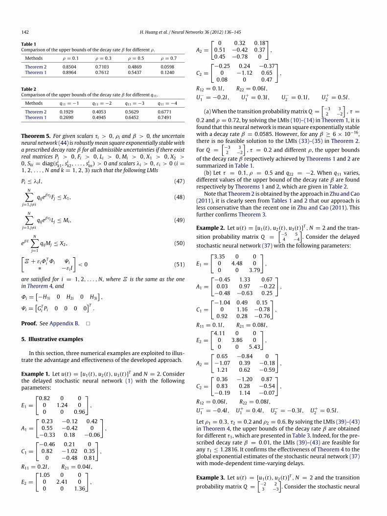
Table 1Comparison of the upper bounds of the decay rate β for different ρ.

Methods ρ = 0.1 ρ = 0.3 ρ = 0.5 ρ = 0.7

Theorem 2 0.8504 0.7103 0.4869 0.0598Theorem 1 0.8964 0.7612 0.5437 0.1240

Table 2Comparison of the upper bounds of the decay rate β for different q11 .

Methods q11 = −1 q11 = −2 q11 = −3 q11 = −4

Theorem 2 0.1929 0.4053 0.5629 0.6771Theorem 1 0.2690 0.4945 0.6452 0.7491

Theorem 5. For given scalars τi > 0, ρi and β > 0, the uncertainneural network (44) is robustlymean square exponentially stablewitha prescribed decay rate β for all admissible uncertainties if there existreal matrices Pi > 0, Fi > 0, Li > 0,Mi > 0, X1 > 0, X2 >0, Ski = diag(sik1, s

ik2, . . . , s

ikn) > 0 and scalars λi > 0, εi > 0 (i =

1, 2, . . . ,N and k = 1, 2, 3) such that the following LMIs

Pi ≤ λiI, (47)N

j=1,j=i

qijeβτjFj ≤ X1, (48)

Nj=1,j=i

qijeβτjLj ≤ Mi, (49)

eβτNj=1

qijMj ≤ X2, (50)

Ξ + εiΦ

Ti Φi Ψi

∗ −εiI

< 0 (51)

are satisfied for i = 1, 2, . . . ,N, where Ξ is the same as the onein Theorem 4, and

Φi =−H1i 0 H2i 0 H3i

,

Ψi =GTi Pi 0 0 0 0

T.

Proof. See Appendix B.

5. Illustrative examples

In this section, three numerical examples are exploited to illus-trate the advantage and effectiveness of the developed approach.

Example 1. Let u(t) = [u1(t), u2(t), u3(t)]T and N = 2. Considerthe delayed stochastic neural network (1) with the followingparameters:

E1 =

0.82 0 00 1.24 00 0 0.96

,

A1 =

0.23 −0.12 0.420.55 −0.42 0

−0.33 0.18 −0.06

,

C1 =

−0.46 0.21 00.82 −1.02 0.350 −0.48 0.81

,

R11 = 0.2I, R21 = 0.04I,

E2 =

1.05 0 00 2.41 00 0 1.36

,

A2 =

0 0.32 0.180.51 −0.42 0.370.45 −0.78 0

,

C2 =

−0.25 0.24 −0.37

0 −1.12 0.650.08 0 0.47

,

R12 = 0.1I, R22 = 0.06I,U−

1 = −0.2I, U+

1 = 0.3I, U−

2 = 0.1I, U+

2 = 0.5I.

(a)When the transition probabilitymatrixQ =

−3 32 −2

, τ =

0.2 and ρ = 0.72, by solving the LMIs (10)–(14) in Theorem 1, it isfound that this neural network ismean square exponentially stablewith a decay rate β = 0.0585. However, for any β ≥ 6 × 10−16,there is no feasible solution to the LMIs (33)–(35) in Theorem 2.For Q =

−3 32 −2

, τ = 0.2 and different ρ, the upper bounds

of the decay rate β respectively achieved by Theorems 1 and 2 aresummarized in Table 1.

(b) Let τ = 0.1, ρ = 0.5 and q22 = −2. When q11 varies,different values of the upper bound of the decay rate β are foundrespectively by Theorems 1 and 2, which are given in Table 2.

Note that Theorem2 is obtained by the approach in Zhu and Cao(2011), it is clearly seen from Tables 1 and 2 that our approach isless conservative than the recent one in Zhu and Cao (2011). Thisfurther confirms Theorem 3.

Example 2. Let u(t) = [u1(t), u2(t), u3(t)]T ,N = 2 and the tran-sition probability matrix Q =

−5 54 −4

. Consider the delayed

stochastic neural network (37) with the following parameters:

E1 =

3.35 0 00 4.48 00 0 3.79

,

A1 =

−0.45 1.33 0.670.03 0.97 −0.22

−0.48 −0.63 0.25

,

C1 =

−1.04 0.49 0.15

0 1.16 −0.780.92 0.28 −0.76

,

R11 = 0.1I, R21 = 0.08I,

E2 =

4.11 0 00 3.86 00 0 5.43

,

A2 =

0.65 −0.84 0−1.07 0.39 −0.181.21 0.62 −0.59

,

C2 =

0.36 −1.20 0.870.83 0.28 −0.54

−0.19 1.14 −0.07

,

R12 = 0.06I, R22 = 0.08I,U−

1 = −0.4I, U+

1 = 0.4I, U−

2 = −0.3I, U+

2 = 0.5I.

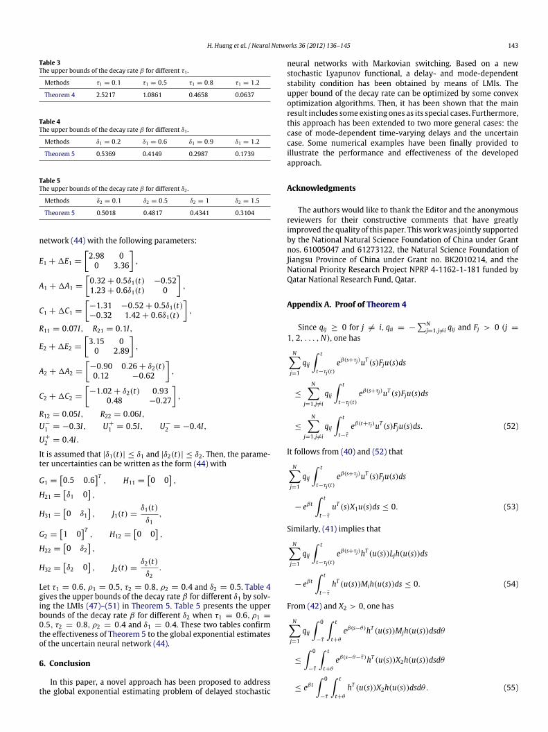
Let ρ1 = 0.3, τ2 = 0.2 and ρ2 = 0.6. By solving the LMIs (39)–(43)in Theorem 4, the upper bounds of the decay rate β are obtainedfor different τ1, which are presented in Table 3. Indeed, for the pre-scribed decay rate β = 0.01, the LMIs (39)–(43) are feasible forany τ1 ≤ 1.2816. It confirms the effectiveness of Theorem 4 to theglobal exponential estimates of the stochastic neural network (37)with mode-dependent time-varying delays.

Example 3. Let u(t) = [u1(t), u2(t)]T ,N = 2 and the transitionprobability matrix Q =

−2 23 −3

. Consider the stochastic neural

H. Huang et al. / Neural Networks 36 (2012) 136–145 143

Table 3The upper bounds of the decay rate β for different τ1 .

Methods τ1 = 0.1 τ1 = 0.5 τ1 = 0.8 τ1 = 1.2

Theorem 4 2.5217 1.0861 0.4658 0.0637

Table 4The upper bounds of the decay rate β for different δ1 .

Methods δ1 = 0.2 δ1 = 0.6 δ1 = 0.9 δ1 = 1.2

Theorem 5 0.5369 0.4149 0.2987 0.1739

Table 5The upper bounds of the decay rate β for different δ2 .

Methods δ2 = 0.1 δ2 = 0.5 δ2 = 1 δ2 = 1.5

Theorem 5 0.5018 0.4817 0.4341 0.3104

network (44) with the following parameters:

E1 + 1E1 =

2.98 00 3.36

,

A1 + 1A1 =

0.32 + 0.5δ1(t) −0.521.23 + 0.6δ1(t) 0

,

C1 + 1C1 =

−1.31 −0.52 + 0.5δ1(t)−0.32 1.42 + 0.6δ1(t)

,

R11 = 0.07I, R21 = 0.1I,

E2 + 1E2 =

3.15 00 2.89

,

A2 + 1A2 =

−0.90 0.26 + δ2(t)0.12 −0.62

,

C2 + 1C2 =

−1.02 + δ2(t) 0.93

0.48 −0.27

,

R12 = 0.05I, R22 = 0.06I,U−

1 = −0.3I, U+

1 = 0.5I, U−

2 = −0.4I,

U+

2 = 0.4I.

It is assumed that |δ1(t)| ≤ δ1 and |δ2(t)| ≤ δ2. Then, the parame-ter uncertainties can be written as the form (44) with

G1 =0.5 0.6

T, H11 =

0 0

,

H21 =δ1 0

,

H31 =0 δ1

, J1(t) =

δ1(t)δ1

,

G2 =1 0

T, H12 =

0 0

,

H22 =0 δ2

,

H32 =δ2 0

, J2(t) =

δ2(t)δ2

.

Let τ1 = 0.6, ρ1 = 0.5, τ2 = 0.8, ρ2 = 0.4 and δ2 = 0.5. Table 4gives the upper bounds of the decay rate β for different δ1 by solv-ing the LMIs (47)–(51) in Theorem 5. Table 5 presents the upperbounds of the decay rate β for different δ2 when τ1 = 0.6, ρ1 =

0.5, τ2 = 0.8, ρ2 = 0.4 and δ1 = 0.4. These two tables confirmthe effectiveness of Theorem 5 to the global exponential estimatesof the uncertain neural network (44).

6. Conclusion

In this paper, a novel approach has been proposed to addressthe global exponential estimating problem of delayed stochastic

neural networks with Markovian switching. Based on a newstochastic Lyapunov functional, a delay- and mode-dependentstability condition has been obtained by means of LMIs. Theupper bound of the decay rate can be optimized by some convexoptimization algorithms. Then, it has been shown that the mainresult includes someexisting ones as its special cases. Furthermore,this approach has been extended to two more general cases: thecase of mode-dependent time-varying delays and the uncertaincase. Some numerical examples have been finally provided toillustrate the performance and effectiveness of the developedapproach.

Acknowledgments

The authors would like to thank the Editor and the anonymousreviewers for their constructive comments that have greatlyimproved the quality of this paper. Thisworkwas jointly supportedby the National Natural Science Foundation of China under Grantnos. 61005047 and 61273122, the Natural Science Foundation ofJiangsu Province of China under Grant no. BK2010214, and theNational Priority Research Project NPRP 4-1162-1-181 funded byQatar National Research Fund, Qatar.

Appendix A. Proof of Theorem 4

Since qij ≥ 0 for j = i, qii = −N

j=1,j=i qij and Fj > 0 (j =

1, 2, . . . ,N), one has

Nj=1

qij

t

t−τj(t)eβ(s+τj)uT (s)Fju(s)ds

≤

Nj=1,j=i

qij

t

t−τj(t)eβ(s+τj)uT (s)Fju(s)ds

≤

Nj=1,j=i

qij

t

t−τ

eβ(t+τj)uT (s)Fju(s)ds. (52)

It follows from (40) and (52) that

Nj=1

qij

t

t−τj(t)eβ(s+τj)uT (s)Fju(s)ds

− eβt t

t−τ

uT (s)X1u(s)ds ≤ 0. (53)

Similarly, (41) implies that

Nj=1

qij

t

t−τj(t)eβ(s+τj)hT (u(s))Ljh(u(s))ds

− eβt t

t−τ

hT (u(s))Mih(u(s))ds ≤ 0. (54)

From (42) and X2 > 0, one has

Nj=1

qij

0

−τ

t

t+θ

eβ(s−θ)hT (u(s))Mjh(u(s))dsdθ

≤

0

−τ

t

t+θ

eβ(s−θ−τ )hT (u(s))X2h(u(s))dsdθ

≤ eβt 0

−τ

t

t+θ

hT (u(s))X2h(u(s))dsdθ. (55)

144 H. Huang et al. / Neural Networks 36 (2012) 136–145

That is,Nj=1

qij

0

−τ

t

t+θ

eβ(s−θ)hT (u(s))Mjh(u(s))dsdθ

−eβt 0

−τ

t

t+θ

hT (u(s))X2h(u(s))dsdθ ≤ 0. (56)

Construct a stochastic Lyapunov functional for each i ∈ S asV (ut , t, i) = eβtuT (t)Piu(t)

+

t

t−τi(t)eβ(s+τi)uT (s)Fiu(s)ds

+

0

−τ

t

t+θ

eβ(s−θ)uT (s)X1u(s)dsdθ

+

t

t−τi(t)eβ(s+τi)hT (u(s))Lih(u(s))ds

+

0

−τ

t

t+θ

eβ(s−θ)hT (u(s))Mih(u(s))dsdθ

+

0

−τ

0

θ

t

t+γ

eβ(s−γ )hT (u(s))

× X2h(u(s))dsdγ dθ. (57)By taking the infinitesimal operator on V (ut , t, i) and noting (15),(53), (54) and (56), one can derive thatL V (ut , t, i) ≤ βeβtuT (t)Piu(t) + 2eβtuT (t)Pi

×−Eiu(t) + Aif (u(t)) + Cih(u(t − τi(t)))

+ eβtTr[σ T (t, i)Piσ(t, i)]

+ eβtNj=1

qijuT (t)Pju(t) + eβ(t+τi)uT (t)Fiu(t)

− (1 − ρi)eβtuT (t − τi(t))Fiu(t − τi(t))

+

Nj=1

qij

t

t−τj(t)eβ(s+τj)uT (s)Fju(s)ds

+ β1eβtuT (t)X1u(t) − eβt t

t−τ

uT (s)X1u(s)ds

+ eβ(t+τi)hT (u(t))Lih(u(t))− (1 − ρi)eβthT (u(t − τi(t)))Lih(u(t − τi(t)))+ β1eβthT (u(t))Mih(u(t))

+

Nj=1

qij

t

t−τj(t)eβ(s+τj)hT (u(s))Ljh(u(s))ds

+ β2eβthT (u(t))X2h(u(t))

− eβt t

t−τ

hT (u(s))Mih(u(s))ds

− eβt 0

−τ

t

t+θ

hT (u(s))X2h(u(s))dsdθ

+

Nj=1

qij

0

−τ

t

t+θ

eβ(s−θ)hT (u(s))

×Mjh(u(s))dsdθ

≤ eβtηT (t)Ξη(t), (58)where η(t) =

uT (t), uT (t − τi(t)), f T (u(t)), hT (u(t)), hT (u(t −

τi(t)))T.

It follows from Ξ < 0 that L V (ut , t, i) ≤ 0 for any η(t).Then, by following the similar line of the proof of Theorem 1, onecan arrive at the conclusion. This completes the proof.

Appendix B. Proof of Theorem 5

To prove Theorem 5, the following lemma is needed:

Lemma 1 (Xie, Fu, & de Souza, 1992). Let Λ1, Λ2, Λ3 be realmatrices of appropriate dimensionswithΛ1 satisfying Λ1 = ΛT

1 , then

Λ1 + Λ2J(t)Λ3 + ΛT3 J

T (t)ΛT2 < 0 for all JT (t)J(t) ≤ I,

if and only if there exists a scalar ε > 0 such that

Λ1 + ε−1Λ2Λ2T

+ εΛT3Λ3 < 0.

Now, respectively replacing Ei, Ai, Ci in (43) by Ei + 1Ei, Ai +

1Ai, Ci + 1Ci yields

Ξ + ΨiJi(t)Φi + ΦTi J

Ti (t)Ψ T

i < 0. (59)

By Lemma1, there exists a scalar εi > 0 such that (59) is equivalentto

Ξ + ε−1i ΨiΨ

Ti + εiΦ

Ti Φi < 0. (60)

Then, by using the Schur complement, (60) is equivalent to (51).Therefore, based on Theorem 4, the uncertain neural network (44)is robustly mean square exponentially stable with a prescribeddecay rate β for all admissible uncertainties. This completes theproof.

References

Ariba, Y., & Gouaisbaut, F. (2007). Delay-dependent stability analysis of linearsystems with time-varying delay. In Proc. of the 46th IEEE conf. on decision andcontrol (pp. 2053–2058). New Orleans, LA, UAS.

Balasubramaniam, P., & Lakshmanan, S. (2009). Delay-range dependent stabilitycriteria for neural networks with Markovian jumping parameters. NonlinearAnalysis: Hybrid Systems, 3, 749–756.

Blythe, S., Mao, X., & Shah, A. (2001). Razumikhin-type theorems on stability ofstochastic neural networks with delays. Stochastic Analysis and Applications, 19,85–101.

Boyd, S., El Ghaoui, L., Feron, E., & Balakrishnan, V. (1994). Linear matrix inequalitiesin system and control theory. Philadelphia, PA: SIAM.

Chen, W., & Zheng, W. X. (2010). Robust stability analysis for stochastic neuralnetworks with time-varying delay. IEEE Transactions on Neural Networks, 21(3),508–514.

Faydasicok, O., & Arik, S. (2012). Robust stability analysis of a class of neuralnetworks with discrete time delays. Neural Networks, 29–30, 52–59.

Haykin, S. (1999). Neural networks: a comprehensive foundation (2nd ed.). UpperSaddle River, NJ: Prentice-Hall.

Huang, H., Ho, D. W. C., & Qu, Y. (2007). Robust stability of stochastic delayedadditive neural networks with Markovian switching. Neural Networks, 20,799–809.

Liao, X., & Mao, X. (1996). Exponential stability and instability of stochastic neuralnetworks. Stochastic Analysis and Applications, 14, 165–185.

Li, X., Gao, H., & Yu, X. (2011). A unified approach to the stability of generalizedstatic neural networks with linear fractional uncertainties and delays. IEEETransactions on Systems, Man and Cybernetics, Part B (Cybernetics), 41(5),1275–1286.

Liu, X., Chen, T., Cao, J., & Lu, W. (2011). Dissipativity and quasi-synchronizationfor neural networkswith discontinuous activations and parametermismatches.Neural Networks, 24, 1013–1021.

Liu, H., Ou, Y., Hu, J., & Liu, T. (2010). Delay-dependent stability analysis forcontinuous-time BAM neural networks with Markovian jumping parameters.Neural Networks, 23, 315–321.

Liu, Y., Wang, Z., Liang, J., & Liu, X. (2009). Stability and synchronization of discrete-time Markovian jumping neural networks with mixed mode-dependent timedelays. IEEE Transactions on Neural Networks, 20(7), 1102–1116.

Liu, Y.,Wang, Z., & Liu, X. (2008). On delay-dependent robust exponential stability ofstochastic neural networks with mixed time delays and Markovian switching.Nonlinear Dynamics, 54, 199–212.

Lou, X., & Cui, B. (2007). Stochastic exponential stability forMarkovian jumpingBAMneural networks with time-varying delays. IEEE Transactions on Systems, Manand Cybernetics, Part B (Cybernetics), 37(3), 713–719.

Ma, Q., Xu, S., Zou, Y., & Lu, J. (2011). Stability of stochastic Markovian jump neuralnetworks with mode-dependent delays. Neurocomputing , 74, 2157–2163.

Mao, X. (2002). Exponential stability of stochastic delay interval systemswith Markovian switching. IEEE Transactions on Automatic Control, 47(10),1604–1612.

Mao, X., Matasov, A., & Piunovskiy, A. B. (2000). Stochastic differential delayequations with Markovian switching. Bernoulli, 6(1), 73–90.

H. Huang et al. / Neural Networks 36 (2012) 136–145 145

Marco, M. D., Grazzini, M., & Pancioni, L. (2011). Global robust stability criteria forinterval delayed full-range cellular neural networks. IEEE Transactions on NeuralNetworks, 22(4), 666–671.

Roska, T., & Chua, L. O. (1992). Cellular neural networks with nonlinear anddelay-type template. International Journal of Circuit Theory and Applications, 20,469–481.

Shen, Y., & Wang, J. (2007). Noise-induced stabilization of the recurrentneural networks with mixed time-varying delays and Markovian-switchingparameters. IEEE Transactions on Neural Networks, 18(6), 1857–1862.

Shu, Z., & Lam, J. (2008). Global exponential estimates of stochastic interval neuralnetworkswith discrete and distributed delays.Neurocomputing , 71, 2950–2963.

Skorohod, A. V. (1989). Asymptotic methods in the theory of stochastic differentialequations. Providence, RI: Amer. Math. Soc.

Tino, P., Cernansky, M., & Benuskova, L. (2004). Markovian architectural bias ofrecurrent neural networks. IEEE Transactions on Neural Networks, 15(1), 6–15.

Wang, Z., Liu, Y., Li, M., & Liu, X. (2006). Stability analysis for stochasticCohen–Grossberg neural networks with mixed time delays. IEEE Transactionson Neural Networks, 17, 814–820.

Wang, Z., Liu, Y., Yu, L., & Liu, X. (2006). Exponential stability of delayed recurrentneural networks with Markovian jumping parameters. Physics Letters A, 356,346–352.

Wu, M., Liu, F., Shi, P., He, Y., & Yokoyama, R. (2008). Exponential stability analysisfor neural networks with time-varying delay. IEEE Transactions on Systems, Manand Cybernetics, Part B (Cybernetics), 38(4), 1152–1156.

Wu, Z., Shi, P., Su, H., & Chu, J. (2011). Delay-dependent stability analysis forswitched neural networks with time-varying delay. IEEE Transactions onSystems, Man and Cybernetics, Part B (Cybernetics), 41(6), 1522–1530.

Wu, Z., Shi, P., Su, H., & Chu, J. (2012). Stability analysis for discrete-timeMarkovianjumpneural networkswithmixed time-delays. Expert Systemswith Applications,39, 6174–6181.

Xie, L., Fu, M., & de Souza, C. E. (1992). H∞ control and quadratic stabilization ofsystems with uncertainty via output feedback. IEEE Transactions on AutomaticControl, 37(8), 1253–1256.

Yang, X., Cao, J., & Lu, J. (2012). Synchronization of Markovian coupled neuralnetworks with nonidentical node-delays and random coupling strengths. IEEETransactions on Neural Networks and Learning Systems, 23(1), 60–71.

Yang, R., Gao, H., & Shi, P. (2009). Novel robust stability criteria for stochasticHopfield neural networks. IEEE Transactions on Systems, Man and Cybernetics,Part B (Cybernetics), 39(2), 467–474.

Zeng, Z., &Wang, J. (2006). Global exponential stability of recurrent neural networkswith time-varying delays in the presence of strong external stimuli. NeuralNetworks, 19, 1528–1537.

Zhang, X., & Han, Q. (2009). New Lyapunov–Krasovskii functionals for globalasymptotical stability of delayed neural networks. IEEE Transactions on NeuralNetworks, 20(3), 533–539.

Zhang, H., Liu, Z., Huang, G., & Wang, Z. (2010). Novel weighting-delay-basedstability criteria for recurrent neural networks with time-varying delay. IEEETransactions on Neural Networks, 21(1), 91–106.

Zhang, H., & Wang, Y. (2008). Stability analysis of Markovian jumping stochasticCohen–Grossberg neural networks with mixed time delays. IEEE Transactionson Neural Networks, 19(2), 366–370.

Zhang, B., Xu, S., Zong, G., & Zou, Y. (2009). Delay-dependent exponentialstability for uncertain stochastic Hopfield neural networks with time-varyingdelays. IEEE Transactions on Circuits and Systems I: Regular Papers, 56(6),1241–1247.

Zheng, C., Zhang, H., & Wang, Z. (2011). Novel exponential stability criteria of high-order neural networks with time-varying delays. IEEE Transactions on Systems,Man and Cybernetics, Part B (Cybernetics), 41(2), 486–496.

Zhu, Q., & Cao, J. (2010). Robust exponential stability of Markovian jump impulsivestochastic Cohen–Grossberg neural networks with mixed time delays. IEEETransactions on Neural Networks, 21(8), 1314–1325.

Zhu, Q., & Cao, J. (2011). Exponential stability of stochastic neural networks withboth Markovian jump parameters and mixed time delays. IEEE Transactions onSystems, Man and Cybernetics, Part B (Cybernetics), 41(2), 341–353.