Evaluating Wireless Sensor Node Longevity through

Markovian Techniques

Dario Bruneo, Salvatore Distefano, Francesco Longo, Antonio Puliafito,Marco Scarpa

Dipartimento di Matematica, Universita di Messina

Contrada di Dio, S. Agata, 98166 Messina, Italia.

Email: {dbruneo,sdistefano,flongo,apuliafito,mscarpa}@unime.it

Abstract

Wireless sensor networks are constituted of a large number of tiny sensor

nodes randomly distributed over a geographical region. In order to reduce

power consumption, nodes undergo active-sleep periods that, on the other

hand, limit their ability to send/receive data. The aim of this paper is to

analyze the longevity of a battery-powered sensor node. A battery discharge

model able to capture both linear and non linear discharge processes is pre-

sented. Then, two different models are proposed to investigate the longevity,

in terms of reliability, of sensor nodes with active-sleep cycles. The first

model, well known in the literature, is based on the Markov reward theory

and on the evaluation of the accumulated reward distribution. The second

model, based on continuous phase type distributions and Kronecker algebra,

represents the main contribution of the present work, since it allows to relax

some assumptions of the Markov reward model, thus increasing its applica-

bility to more concrete use cases. In the final part of the paper, the results

obtained by applying the two techniques to a case study are compared in

order to validate and highlight the benefits of our approach and demonstrate

Preprint submitted to Computer Networks July 20, 2011

the utility of the proposed model in a quite complex and real scenario.

Keywords: Wireless sensor networks, Longevity, Reliability, Energy

consumption, Battery discharge process, Markov reward models,

Continuous phase type distributions, Kronecker algebra.

1. Introduction

Wireless sensor networks (WSN) are networks composed of tiny sensors

equipped with radio interfaces and distributed over a geographical region.

The task of each sensor is to perform measurements and to send data to a

node collector or sink. The WSN application areas are numerous and differ-

ent, ranging from disaster recovery to field monitoring. Interesting applica-

tions have also been found in industrial scenarios where hostile environments

can preclude the human intervention or the deployment of networking infras-

tructures.

In the last years, researches on WSN have mainly focused on networking

aspects [1, 2] as well as on data management [3]. However, many specific

applications introduce strict dependability requirements [4, 5] that are pri-

marily related to data security and reliability [6] and to the longevity of the

single node and the WSN as whole [7, 8, 9, 10, 11]. In fact, in this latter

case, cheap sensors do not guarantee their functioning over the time and they

are normally equipped with low voltage batteries that limit their lifetime or

longevity. From such perspective, a WSN is a power constrained system,

since nodes run on limited power batteries.

In order to reduce and optimize the energy consumption, a common prac-

tice is to switch WSN nodes into a lower powered state, usually identified as

2

sleep mode, by deactivating the radio equipments when no data have to be

transmitted [7]. Since quite often the radio is the highest power consumer

subsystem in a WSN node, this allows to save battery and therefore to im-

prove the node lifetime. In this way, by associating the battery discharge

to the WSN node aging process as in [7, 8, 9], the node longevity can be

expressed, in terms of reliability, as a function of the battery state of charge.

Several authors deal with WSN and power management topics, at differ-

ent layers and achieving different goals. In the specific context of reliability,

an interesting investigation is performed in [9], where a simulation technique

for evaluating blind flooding over WSN is proposed. The authors base the

evaluation on a realistic and accurate battery model, also considering capac-

ity and recovery effects as well as switching energy, instead of starting from

the linear discharge model usually assumed in literature.

The choice of the battery model is of primary importance in evaluating

the WSN longevity as also highlighted in [10]. Mathematical models [12]

apply empirical equations to address the battery charge/discharge behavior;

electrochemical models [13] provide a more detailed representation of the

process but, on the other hand, they usually require greater efforts in their

evaluation; electrical models [14] are instead mainly used for circuit analysis,

simulation and optimization.

Mathematical battery models are usually used in the node/WSN longevity

and power management modeling and evaluation. For example, in [11] a new

sensor node deployment scheme is proposed to increase the sensor network

longevity assuming a non-linear battery discharge model. More recently, [10]

proposes a flexible and extensible simulation framework to estimate power

3

consumption of sensor network applications for arbitrary hardware platforms

in which energy and timing parameters are partially obtained through direct

measurements.

The problem of WSN longevity and power management has also been

investigated through the use of analytical models. For example, in [8] Markov

models are used in order to evaluate WSN reliability. In such case the context

is slightly different: WSN composed of several nodes are considered and

the final model reflects such choice, representing the WSN as a whole and

introducing some higher level approximations.

The aim of this work is to analyze the longevity of a single WSN node

undergoing cycles of active-sleep periods. Both linear and non linear bat-

tery models are taken into consideration, thus proposing and comparing two

different analytical techniques. The former is based on a Markov reward

model able to capture the linear battery depletion process of a WSN node

and to derive the reliability parameters under specific assumptions. The lat-

ter is based on continuous phase type distributions (CPHs) and Kronecker

algebra and is able to relax some of the assumptions related to the Markov

reward solution technique. In particular, non linear battery discharge model

and different active-sleep modes sojourn time distributions can be taken into

account. Moreover, some numerical problems that could affect the imple-

mentation of the first technique can be overcome by our approach.

From an operational/practical viewpoint, the proposed technique can be

exploited to perform parametric evaluations on the WSN also taking into

account the application requirements, as for example: finding out the ap-

propriate duty cycle to be used for achieving the expected lifetime required

4

by the application, deriving the expected node’s lifetime, depending on its

assigned duty cycle, etc.

The paper is organized as follows: Section 2 introduces and discusses

the battery discharge phenomena, also proposing a possible model and its

validation. Section 3 describes WSN nodes characterizing the problem under

evaluation. In Section 4 a Markov reward model of a WSN node is described,

while in Section 5 a technique based on CPHs and Kronecker algebra is

detailed. From the evaluation of such models specific results are obtained,

compared and discussed in Section 6, while Section 7 concludes the paper

with final remarks and future work.

2. Battery discharge model

As stated above, WSN can be considered as power-constrained systems in

which the power management problem has to be adequately addressed. It is

therefore required to use adequate techniques and models in order to satisfy

and optimize the power management, also taking into account the applica-

tion requirements and specifications. With regards to batteries, that usually

provide the WSN power supply system, it is necessary to define adequate

models to describe their discharge process.

The battery lifetime or time-to-failure is the time to discharge. Once

the battery is exhausted the powered system, in the specific the WSN node,

shuts down; therefore, maximizing the battery lifetime is an important goal

to be addressed.

Starting from the existing literature [9, 15], one of the most adopted

analytical models to represent the discharge process of a battery subjected

5

to a constant load is based on the Peukert’s law [16] that expresses the

capacity of a battery in terms of the rate at which it is discharged: if the

rate increases, the available charge capacity decreases. Generally such effect

can be quantified by the formula:

T = H ·

(

C

H · I

)η

(1)

that analytically formalizes the relationships among the time of discharge

T , expressed in hours, the rated capacity of the battery C at the specified

hour rating H (hours), expressed in Ampere·hours and the (constant) dis-

charge current I, expressed in Ampere. In (1) η is the Peukert’s exponent

or constant, ranging in the interval [1, 2], depending on the chemical process

characterizing the battery. The Peukert constant increases with age for any

of the battery types, but generally ranges from [1.05, 1.15] for lead-acid bat-

teries, [1.1, 1.25] for gel, [1.2, 1.6] for flooded batteries, [1.06, 1.13] for lithium

ion batteries while [1.2, 1.4] characterizes alkaline batteries. A value of η

equal to 1 identifies the ideal case, in which the discharge process is linear,

i.e., the battery capacity C linearly decreases with the current I. In such

case the actual capacity would be independent of the current.

The Peukert’s law expresses the battery lifetime given an initial capacity.

In the proposed modeling technique, we need to know the trend of the battery

discharge process with respect to the time. To this end, by inverting eq. (1)

we can obtain the relationship for the capacity C as follows:

C = I ·H ·

(

T

H

)(1/η)

. (2)

6

Then, considering C as a function of the time variable t, we can express its

evolution in time as c(t) from eq. (2):

c(t) = c0 − I ·H ·

(

t

H

)(1/η)

(3)

where c0 is the initial capacity of the battery.

...

...Figure 1: Discharge curve of a battery subject to a constant load.

By eq. (3) we can argue that, when a constant load is applied, a time-

varying discharge rate commonly characterizes the batteries discharge pro-

cess. A typical trend of the discharge process in time c(t) is shown in Figure 1.

Since such trend is not linear, it is necessary to recur to an adequate model

to represent it. Let us identify the battery useful charge range as [c0, cmin],

that we split into n contiguous intervals [ci, ci+1] of equal sizec0−cmin

n, with

i = 0, . . . , n − 1. In this way, we discretize the battery capacity into n + 1

charge levels with generic value ci (i = 0, . . . , n), where cn = cmin. Since

c(t) is usually strictly decreasing, the time instants ti such that c(ti) = ci,

with i = 0, . . . , n, can be univocally identified. Let τi = ti+1 − ti, with

7

i = 0, . . . , n−1, be the duration of the i-th time interval, in which the charge

assumes values ranging into [ci, ci+1]. By discretizing the value assumed by

the charge in [ti, ti+1] with ci, we can represent the discharge phenomenon

through the n + 1-state continuous time Markov chain (CTMC) shown in

Figure 2 and defined by the stochastic process

B = {B(t), t ≥ 0} (4)

where the state bi encodes the i-th charge interval. Since ∀t ∈ [ti, ti+1] ⇒

c(t) ∈ [ci, ci+1], τi can be considered as the sojourn time into the state bi and,

as a consequence, the transition rate between states bi and bi+1 has to be set

to λi =1τi.

...

Figure 2: CTMC representing the battery discharge process of Figure 1.

The introduced model is a CTMC with an absorbing state whose absorp-

tion time is a random variable that represents the time-to-discharge of the

battery. As a consequence, the distribution of the time to absorption of the

CTMC represents the distribution of the time-to-discharge. The CTMC thus

obtained describes a single discharge behavior corresponding to a constant

load; if different loads have to be considered, as a number of CTMCs equal

to the number of different loads have to be specified accordingly. Anyway, all

the CTMCs modeling the battery discharge in the different load conditions

are characterized by the same number of states if the discretization levels are

the same; considering the same battery this is not a restrictive assumption,

8

since the initial charge level c0 and its minimum cmin are fixed for a given

battery. The sojourn time into each state of the chain of Figure 2 has been

considered as exponentially distributed because our aim is to characterize the

function describing the discharge process of the sensor node battery through

a CPH distribution. Such a characterization allows us to approximate a non-

Markovian stochastic process with an expanded CTMC that captures the

discharge process of the sensor node.

2.1. Validating the battery discharge model

In order to validate the CPH battery discharge model proposed we solved

the CTMC depicted in Figure 2 and compared the results against the battery

discharge function c(t) obtained by the Peukert’s law expressed in eq. (3).

More formally, we obtained an estimation c(t) of the c(t) function as the

expected value of the stochastic process B of eq. (4) at time t:

c(t) =n

∑

i=0

ci ∗ Pr{B(t) = bi}. (5)

We also evaluated an estimation of the total battery depletion distribution

F (t) as the probability the CTMC is in the absorbing state, i.e., the prob-

ability for the battery to be depleted at time t. Such function is compared

with the F (t) that is defined as:

F (t) =

1 if t ≤ T

0 if t > T(6)

where T is the battery lifetime expressed in eq. (1).

9

0

500

1000

1500

2000

2500

0 5 10 15 20 25 30 35

c(t)

,c-(t

)

Time (h)

c-(t) with n=25c-(t) with n=100

c-(t) with n=1000c(t)

(a)

0

0.2

0.4

0.6

0.8

1

0 10 20 30 40 50

F(t

), F- (t

)

Time (h)

F-(t) with n=25

F-(t) with n=100

F-(t) with n=1000

F(t)

(b)

Figure 3: Battery discharge function (a) and corresponding total depletion time distribu-tion (b) varying the number of states.

Figure 3 shows the obtained results. We referred to an alkaline battery

(AA/R6) with Peukert constant η = 1.3, initial capacity c0 = 2500mAh,

constant load I = 100mA and, consequently, H is 25h. As expected, by

increasing the number n of states of the CTMC, we obtained a better ap-

proximation. In particular, it can be observed that with a 1000 states-CTMC

we obtain a very good approximation of the battery discharge process.

3. Longevity of WSN nodes with active-sleep cycles

In typical WSN applications, wireless sensor nodes are randomly scat-

tered in large geographical regions and it is not always possible to perform

node maintenance after the WSN deployment by intervening on the single

node. For this reason, sensor nodes have to adapt their behavior to the

environmental changes. In particular, each node has to reduce its power con-

sumption in order to increase the WSN lifetime. Sensor nodes are usually

powered by low voltage batteries and they are composed of a processing unit,

a wireless communication unit, and a sensing unit. Wireless communications

10

represent the most expensive task a node has to accomplish [7], but even if

no data are actually transmitted, the energy consumed by the wireless com-

munication unit is significant. Then, in order to reduce energy consumption,

a good strategy is to deactivate the radio equipments when no data have to

be transmitted. According to this strategy, nodes periodically go through

two different functioning states: active and sleep. When the node is in the

active state, it is able to send/receive data while, when sleeping, it is only

able to perform off-line tasks such as sensing and data processing.

In order to analyze the battery discharge process of a node with active-

sleep cycles, it is possible to associate to each operating mode the corre-

sponding battery discharge function c(t). Being the discharge process strictly

related to the battery type, functions c(t) associated to different operating

modes have the same value of η and H of eq. (3) and only differ in the

discharge current I.

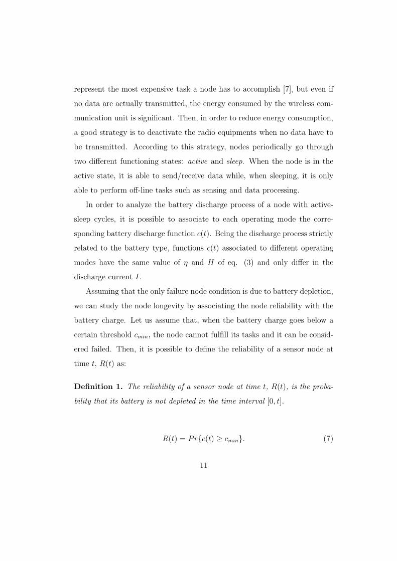
Assuming that the only failure node condition is due to battery depletion,

we can study the node longevity by associating the node reliability with the

battery charge. Let us assume that, when the battery charge goes below a

certain threshold cmin, the node cannot fulfill its tasks and it can be consid-

ered failed. Then, it is possible to define the reliability of a sensor node at

time t, R(t) as:

Definition 1. The reliability of a sensor node at time t, R(t), is the proba-

bility that its battery is not depleted in the time interval [0, t].

R(t) = Pr{c(t) ≥ cmin}. (7)

11

In the following, starting from the battery discharge model presented in

Section 2 and knowing the energy consumption parameters associated to the

two operating modes and the period of the active-sleep cycles, we show how

the reliability function R(t), and then the node longevity, can be evaluated.

This paper has been focused on the reliability distribution of a single

sensor node. Once such distribution is obtained it is possible to extend the

investigation to the WSN as a whole. Two possible cases can be identified. If

the failure events (in this case the battery discharge) are statistically indepen-

dent the reliability of the whole WSN can be obtained using combinatorial

techniques such as fault trees. We focused on this aspect on [17, 18]. If the

failure events are statistically dependent the reliability of WSN can be stud-

ied using dynamic reliability tools such DRBD [19] or modeling techniques

able to capture the interactions among sensors, such as Markovian Agents

[20]. We plan to investigate such a second aspect in future works.

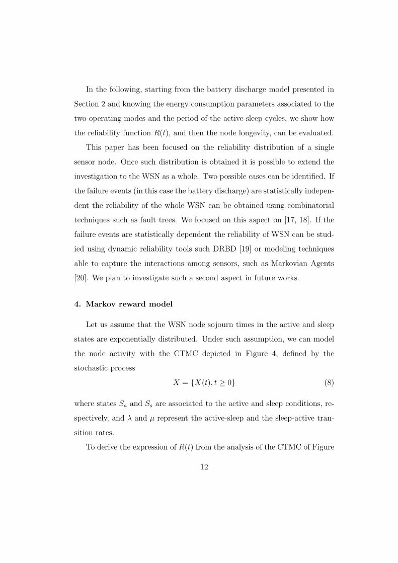
4. Markov reward model

Let us assume that the WSN node sojourn times in the active and sleep

states are exponentially distributed. Under such assumption, we can model

the node activity with the CTMC depicted in Figure 4, defined by the

stochastic process

X = {X(t), t ≥ 0} (8)

where states Sa and Ss are associated to the active and sleep conditions, re-

spectively, and λ and µ represent the active-sleep and the sleep-active tran-

sition rates.

To derive the expression of R(t) from the analysis of the CTMC of Figure

12

Figure 4: CTMC representing the active-sleep cycles of a WSN node.

4 we can recur to the Markov reward theory [21]. Let us associate to states

Sa and Ss indices i = 0 and i = 1, respectively, and let us indicate with

S = {0, 1} the state space associated to the CTMC of the WSN node. Then,

we can define a reward function r : S → R in which, for each state i ∈ S,

r(i) = ri represents the reward obtained per unit time spent by process X in

that state.

We can associate the reward to the battery consumption by defining r as:

ri =

qa if i = 0

qs if i = 1

(9)

where qa and qs represent the charge absorbed by the sensor per unit time in

the active and sleep states, respectively. If the charge absorbed by the node

is not constant over the time [22], it is possible to consider reward functions

r(i, t) that are also time-dependent on time [21].

Let Z(t) = rX(t) be the system reward rate (i.e., the node charge ab-

sorption rate) at time t. We can define the accumulated reward Y (t) in the

interval [0, t) as:

Y (t) =

∫ t

0

Z(τ)dτ. (10)

The value of Y (t) can be interpreted as the charge consumed by the node

13

from the activation instant till time t. By and indicating with c0 the initial

battery charge of the WSN node, from (10) we can express the battery charge

level c(t) at time t as:

c(t) = c0 − Y (t). (11)

An interesting measure to compute is the distribution of the accumulated

reward that can be expressed as:

F (t, y) = Pr{Y (t) ≤ y}. (12)

In fact, from (7), (11), and (12) we can derive the expression of R(t) as:

R(t) = Pr{c(t) ≥ cmin}

= Pr{c0 − Y (t) ≥ cmin}

= Pr{Y (t) ≤ c0 − cmin}

= F (t, c0 − cmin). (13)

Then, to perform a quantitative analysis of R(t), we need to evaluate the

distribution of the accumulated reward F (t, y). Such distribution can be

computed starting from the analysis of the CTMC described in Figure 4.

4.1. Closed-form solution

A method for evaluating F (t, y) during a finite mission time and assuming

the reward rates to be time independent is provided in [23]. If A = [aij ] is

the infinitesimal generator of the process X , it is possible to indicate with

P = [pij] = A/γ + I the stochastic matrix of the associated Poisson process,

14

where γ ≥ max{|aij |} and I is the identity matrix. Then, F (t, y) can be then

expressed as:

F (t, y) =∞∑

k=0

[α(k)0 u(y − r0t) +

k∑

h=1

1∑

w=0

(

k

h− 1

)

·

·β(k)0 (w, h)

(

y − rwt

t

)k−h+1

u(y − rwt)] ·(γt)ke−γt

k!

(14)

where

u(x) =

0 if x < 0

1 if x ≥ 0(15)

and coefficients α(k)i and β

(k)i (w, h) are recursively defined by:

α(k)i =

0 if k = 0

1∑

j=0rj=ri

pijα(k−1)j if k > 0

(16)

β(k)i (w, h) =

−1

∑

j=0rj=rw

pijα(k−1)j

rw − riif w 6= i, h = k

β(k)i (w,h+1)

rw−ri−

∑1j=0

pijβ(k−1)j (w,h)

rw−riif w 6= i, h < k

−

1∑

w=0w 6=i

β(k)i (w, 1) if w = i, h = 1

1∑

j=0

pijβ(k−1)j (i, h− 1) if w = i, h > 1

(17)

15

To numerically solve eq.(14), the infinite sum has to be truncated to a

value k∗ that depends on the required error tolerance. An estimation of the

error truncation is given by:

ε(k∗) ≤ 1− e−γtk∗∑

k=0

(γt)k

k!(18)

5. The CPH distributions and Kronecker algebra model

Eq. (14) cannot be used to compute the WSN node reliability in case of

time dependent reward rates. However, even in the simple case of constant

reward rates, the algorithm that can be used to evaluate eq. (14) and to

compute the recursive coefficients α(k)i and β

(k)i (w, h) could be subject to

numerical problems (overflow, underflow, stiffness). Such issues could prevent

eq. (14) to be used for the computation of the node reliability R(t) for large

values of t.

Moreover, the described technique cannot be used when the relationship

between the charge of the battery and the reliability of the node is more

complex than that of eq. (7): for example if we assume that there is a non-

null probability for the node to fail, even if the battery charge is greater than

cmin. Finally, the stochastic process X could be more complex than a simple

CTMC, being the sojourn times of the node in active and sleep states non-

exponentially distributed. As an example, the sojourn times could depend

on the load of the node in terms of number of packets it is processing at a

specific time instant.

For such reasons we propose an alternative analytical technique based on

CPH distributions and Kronecker algebra. It can be used for evaluating the

16

WSN node reliability relaxing some of the assumptions specified in Section

4.

Figure 5: State space model representing the sensor node lifecycle.

The state space model depicted in Figure 5 represents the behavior of a

sensor node also considering its battery depletion. As in Figure 4, states Sa

and Ss are related to the active and the sleep modes of the WSN node under

exam, respectively, while the absorbing state Sf represents the node failure

due to the battery depletion. Events ea and es are related to the transitions

between active and sleep modes, while event ef represents the failure of the

WSN node.

Let us assume that the cumulative distribution functions (CDFs) Fa(t)

and Fs(t) are associated to events ea and es, while two different time-to-

failure distributions F af (t) and F s

f (t) are associated to event ef in states Sa

and Ss, respectively. F af (t) and F s

f (t) are the node lifetime distributions in

the two functioning states in isolation, as specified in Section 3. They are

obtained from the battery discharge functions of states Sa and Ss as detailed

in Section 2, so both of them are represented by n+ 1 states CTMCs.

Since the WSN node cyclically changes its functioning state triggered by

17

events ea and es, the distribution associated to event ef changes from F af (t)

to F sf (t) and vice-versa. Moreover, at the generic change point t the battery

charge has to be preserved. For example, the changing from F af (t) to F s

f (t) at

t means that the battery discharge process of the node continues according

to F sf (t), thus preserving the battery charge level reached so far, i.e., F a

f (t).

In terms of the battery model introduced in Section 2, the battery charge

level is preserved by the CTMC state reached when F af (t) is disabled at t,

since each state corresponds to a specific charge level.

Based on these considerations, in the following we describe a technique

based on CPH distributions and Kronecker algebra for evaluating such model.

In this way, the unreliability and the sojourn time distribution of the WSN

node in the two functioning modes are represented by CPHs, moving the

problem towards the solution of an expanded CTMC. Kronecker algebra is

therefore used in order to deal with the well-known state space explosion

problem, since this allows the infinitesimal generator matrix of the expanded

CTMC is never generated nor stored as a whole, but it can be algorithmically

evaluated on-the-fly in a block-wise fashion during the model solution. In this

way, only few information about the stochastic process is permanently stored,

with consequent memory saving.

5.1. Representing events through CPHs

The use of phase type (PH) distributions dates back to the pioneering

work of Erlang on congestion in telephone systems at the beginning of the

last century [24] and was popularized in 1981 by Neuts [25] who formally

defined a PH distribution as the distribution of the time until absorption in

a finite state Markov chain with a single absorbing state. In particular, the

18

class of CPH distributions is defined over CTMCs.

More specifically, let us consider a CTMC χ with ℓ transient states and

a single absorbing state (labeled ℓ+ 1) whose infinitesimal generator matrix

G ∈ Rℓ+1 ×R

ℓ+1 is in the form:

G =

G U

0 0

where G ∈ Rℓ × R

ℓ describes the transient behavior of the CTMC and

U ∈ Rℓ is a vector grouping the transition rates to state ℓ + 1. Moreover,

let us suppose that the chain is started with an initial probability vector

π(0) = [α, αℓ+1] such that αℓ+1 = 1−∑ℓ

i=1 αi. We say that a random variable

T is distributed according to the CPH distribution with representation (α,G)

and order ℓ if its CDF FT (t) is the probability to reach the absorbing state

of χ; FT (t) can be expressed as:

FT (t) = 1−α · eGt · 1, t ≥ 0 (19)

The theory of PH distributions found several applications in reliability

(see Neuts [26], Perez-Ocon et al. [27, 28, 29] and references therein) and,

in general, in the analysis of stochastic models where non-exponentially dis-

tributed events are considered. Other interesting and powerful techniques

exist for the analysis of such class of non-Markovian models such as sup-

plementary variables, semi-Markov processes, and Markov regenerative mod-

els [30], but they usually present severe restrictions on the structure of the

manageable systems. On the contrary, the use of PH distributions for the

19

representation of non-exponentially distributed events (state space expansion

approach [25]) allows to manage a more general class of models.

The state space expansion approach consists in the representation of a

non-Markovian stochastic process by mean of a Markov chain defined over an

augmented state space [31]. Each state in the non-Markovian process is ex-

panded into a set of states within the Markov chain, called macro-state, with

the purpose to capture the evolution of the non-exponentially distributed

events within it. In particular, when CPH distributions are used, the non-

Markovian process is represented via an expanded CTMC.

By applying the state space expansion approach to the WSN node under

evaluation, we have to represent Fa(t), Fs(t), Faf (t), and F s

f (t) through CPH

distributions. In such model, special care has to be devoted to the represen-

tation of the node unreliability in the two operating modes, since the charge

level has to be preserved at change points.

5.2. From CPHs to Kronecker algebra

Let us consider a discrete-state discrete-event non-Markovian model and

let S be the system state space and ε the set of system events. Follow-

ing the state space expansion approach, the events are represented by CPH

distributions, and the expanded CTMC thus resulting is composed of ||S||

macro-states, characterized by a ||S|| × ||S|| block infinitesimal generator

matrix Q in which:

• the generic diagonal block Qii (1 < i < ||S||) is a square matrix that

describes the evolution of the CTMC inside the macro-state related to

state i, and it depends on the possible events occurring in that state;

20

• the generic off-diagonal blockQij (1 < i < ||S||, 1 < j < ||S||) describes

the transition from the macro-state related to state i to that related to

state j, and it depends on the event occurred in state i and the possible

events able to still occur in state j.

The main drawback of the state space expansion approach is the explosion

of the state space. This limits the applicability of the approach thus reducing

its benefits and potentialities. A possible solution to overcome the problem

is to recur to Kronecker algebra [25, 32, 28], a well known and effective

technique able to provide a compact representation of CTMCs. Kronecker

algebra is based on two main operators [33]: Kronecker product (⊗) and

Kronecker sum (⊕). Given two rectangular matrices A and B of dimensions

m1×m2 and n1×n2 respectively, their Kronecker product A⊗B is a matrix

of dimensions m1n1 ×m2n2. More specifically, it is a m1 ×m2 block matrix

in which the generic block i, j has dimension n1 × n2 and is given by ai,j ·B.

On the other hand, if A and B are square matrices of dimensions m×m and

n × n respectively, their Kronecker sum A ⊕B is the matrix of dimensions

mn × mn written as A ⊕ B = A ⊗ In + Im ⊗ B where In and Im are the

identity matrices of order n and m, respectively.

By exploiting Kronecker algebra, matrix Q does not need to be generated

and stored as a whole but can be symbolically represented through Kronecker

expressions and algorithmically evaluated on-the-fly when needed [34, 35]. As

detailed below, the matrix Q blocks have the following form:

Qii =⊕

1<e<||ε||

Qe (20)

21

Qij =⊗

1<e<||ε||

Qe (21)

Diagonal blocks are computed as Kronecker sums (off-diagonal blocks are

computed as Kronecker products) of a series of matrices Qe each of which

is associated to one of the system events and depends on the behavior of

such event in the involved states. In this context, operators ⊕ and ⊗ assume

particular meanings. Let us consider two CTMCs χ1 and χ2 with infinitesi-

mal generator matrices Q1 and Q2. The matrix resulting by the Kronecker

sum of these matrices (Q1 ⊕ Q2) is usually interpreted as the infinitesimal

generator matrix of the CTMC that models the concurrent evolution of χ1

and χ2. It is important to remark that the resulting CTMC is composed of

a set of states that derives from the combination of all the states of the two

initial CTMCs.

On the other hand, let us consider a CTMC χ1 with a single absorbing

state and let U be the column vector containing the transition rates to such

state. Moreover, let us consider a CTMC χ2 and let P be a matrix that

contains the probabilities to enter into the χ2 states. The matrix obtained

by the Kronecker product of U and P (U⊗P) is usually interpreted as the

matrix containing the transition rates to the CTMC resulting from the com-

bination of the absorbing state of χ1 with all the states of χ2. For a complete

treatment of all the possible forms of matrices Qe, in the case of discrete-time

models, see [35]. Here, we apply such technique to the evaluation of a WSN

node reliability in order to derive the corresponding Qe matrices.

22

In order to represent the WSN node with active-sleep cycles, let us con-

sider the three states model of Figure 5. In terms of Kronecker algebra terms,

the expanded CTMC, obtained by introducing the sojourn time distributions

in states Sa and Ss and the battery discharge models, is represented by the

infinitesimal generator matrix Q, that is the 3× 3 block matrix:

Q =

Q00 Q01 Q02

Q10 Q11 Q12

Q20 Q21 Q22

where states Sa, Ss and Sf are identified as 0, 1 and 2, respectively.

In the following, (αa,Ga) and (αs,Gs) are the CPH representations of

the node sojourn time CDFs Fa(t) and Fs(t) in the two functioning states,

and (αaf ,G

af) and (αs

f ,Gsf) are the CPH representations of the node time-

to-failure CDFs F af (t) and F s

f (t).

Let us start with the description of the diagonal blocks of matrix Q. In

state Sa, events es and ef are enabled and can evolve concurrently according

with their CPH distributions while event ea is disabled. For such a reason,

matrix Q00 is:

Q00 = Gs ⊕Gaf ⊕ [0] (22)

where matrix [0] (i.e., a matrix with a single element equal to 0) associated to

event ea is the neutral element for the Kronecker sum operator. Similarly, in

state Ss events ea and ef are enabled and can evolve concurrently according

to their CPH distributions while event es is disabled, thus:

Q11 = [0]⊕Gsf ⊕Ga. (23)

23

On the other hand, in state Sf no event is enabled, therefore Q22 is a 1 × 1

null matrix.

With regards to off-diagonal blocks of matrix Q, let us start with matrix

Q01 associated to the transition from Sa to Ss. Event es is enabled in Sa

and causes the state transition, becoming disabled in state Ss. Thus, the

stochastic process leaves the phases of the CPH associated to event es with

the rates specified in Us. On the other hand, ea is disabled in Sa and enabled

in Ss. As a consequence, the stochastic process enters the phases of the CPH

associated to ea with the probabilities given by vector αa. Finally, ef is

enabled in both Sa and Ss but changes its distribution from F af (t) to F s

f (t).

Since, as stated above, the CPHs representing F af (t) and F s

f (t) have been

specified by coding the battery charge levels in their states, and the charge

level has to be preserved changing from Sa to Ss, the (jth) state reached

by the CPH corresponding to F af (t) has to be saved by restarting from the

same state (j) of the CPH corresponding to F sf (t). Such behavior can be

implemented by using an n× n identity matrix Ia→s:

Q01 = Us ⊗ Ia→s ⊗αa. (24)

Similarly Q10, representing the transition from Ss to Sa, has the form:

Q10 = αs ⊗ Is→a ⊗Ua. (25)

The matrix representing the transition from Sa to Sf triggered by the

firing of ef is:

Q02 = es ⊗Uaf ⊗ [1]. (26)

24

since es is enabled in Sa but it is disabled in Sf without firing and it is not

required to keep memory of the state reached (the corresponding matrix is the

column vector es whose elements are equal to 1). Such vector represents the

fact that, regardless of the probabilities to be in a stage of the CPH associated

to the event es, in Sf the failure event disables all the other events.

Matrix [1] (i.e., a matrix with a single element equal to 1) is the neutral

element for the Kronecker product operator and it is associated to ea since

it does not contribute to the state transition, being disabled in both the

involved states and having no memory in the reached state. Event ef is

associated to Uaf since its firing causes the state transition. Similarly, Q12 is

given by:

Q12 = [1]⊗Usf ⊗ ea. (27)

Finally, since Sf is an absorbing state and no event is enabled in it, Q20 and

Q21 are null matrices.

In this way, by applying the CPH-Kronecker algebra technique, the stochas-

tic process underlying the WSN node lifecycle considering non-Markovian

sojourn times and time-to-failure distributions is reduced to a CTMC that

can be easily solved by applying a classical transient solution method (e.g.,

the uniformization method) for the computation of the WSN node reliability

R(t).

6. Numerical results

In this section, we present some numerical results obtained by using the

described techniques. First of all, we provide a comparison between the

Markov reward model and the CPH-Kronecker model in order to demonstrate

25

the equivalence of the two approaches. Then, by evaluating the WSN node

reliability function R(t), we show how to apply the CPH-Kronecker technique

in order to derive important parameters that can be used during the setup

phase of a WSN.

6.1. Techniques comparison

0

0.2

0.4

0.6

0.8

1

0 5 10 15 20 25 30

R(t

)

Time (sec)

CPH approach with n=25CPH approach with n=100

CPH approach with n=1000Markov reward approach

Figure 6: Node reliability R(t) computed with the Markov reward approach and the CPH-Kronecker approach.

In order to demonstrate the equivalence between the modeling techniques

described in the previous sections, we need to take into consideration a sce-

nario that can be analyzed by mean of the Markov reward model. As we have

already discussed, only a linear battery model can be evaluated through the

accumulated reward distribution closed-form equation (14), meaning that

constant reward rates have to be associated to the WSN node active and

sleep modes. Moreover, due to some numerical issues encountered in the im-

plementation of the Markov reward model technique and specifically of eq.

(14), it is not possible to evaluate the WSN node reliability for large values

26

of t and therefore it is not possible to validate the CPH-Kronecher algebra

technique by the previously analyzed scenario.

We thus consider a WSN node characterized by a linear battery discharge

of 10 s in the active mode of and 20 s in the sleep one. The WSN node

lifecycle is regulated by the CTMC depicted in Figure 4 with λ = 1.0 s−1

and µ = 0.2 s−1. In order to apply the CPH-Kronecher technique the WSN

node battery linear discharge process has been approximated by a 1000-phase

CPH.

Figure 6 reports the comparison between the WSN node reliability func-

tion R(t) computed with the Markov reward model and with the CPH-

Kronecker technique varying the number of the CPH phases n. It can be

observed that, in the case of n = 1000, the two curves are totally overlapped

and small differences are present only in the two knees of the curves, thus

demonstrating the effectiveness of the CPH-Kronecker technique and also

validating it.

6.2. Reliability analysis

Once the reliability model has been validated, it is possible to use it in

the evaluation of the WSN sensor node longevity as specified in Section 3

and more specifically by eq. (7). We apply the CPH-Kronecker technique

described in Section 5. The WSN node is therefore characterized by the ac-

tive and sleep states, and it periodically switches between the two operating

modes. The proposed technique is not strictly related to a particular appli-

cation or communication protocol, and it is general enough to be adopted at

large. For this reason, we do not focus on a specific duty cycle period and

the values of parameters λ and µ are specified in order to provide a full nu-

27

merical example. In particular, to derive the expression of R(t), we assume

that the stochastic processes associated to events ea and es of Figure 5 are

exponentially distributed with rates λ = 3600 h−1 and µ = 60 h−1, meaning

that the node switches from active to sleep with a mean time of 1s, while

from sleep to active with a mean time of 60 s.

The battery discharge process has been characterized by using the same

battery parameters listed in Section 2.1. To differentiate the discharge pro-

cesses in the active and sleep modes we have to evaluate the corresponding

energy consumptions in terms of the discharge current I. Starting from

empirical data obtained by experiments on MeshNetics MeshBean2 boards,

we observed that such WSN nodes in the active mode absorb a current

Ia = 100 mA, while in the sleep mode a current Is = 20 mA.

With regard to the CPH-Kronecker model, we can consider the represen-

tation of the battery discharge process shown in Figure 2 as a specific CPH.

As discussed in Section 2, the two CTMCs corresponding to the discharge

from both active and sleep modes have the same number of states or phases

identifying and discretizing the battery charge level reached. They differ only

in the rates between the phases. Thus, to the same i − th phase of the two

CPHs. In such a way the CPH-Kronecker technique described in Section 5

can be applied, keeping memory of the charge level reached by saving the

corresponding CPH phase in the transitions between macrostates involving

active-sleep and sleep-active mode switching.

The results obtained by evaluating the reliability function R(t) through

a 1000 phases CPH model are shown in Figure 7, in the specific the non

linear discharge curve. The resulting function has been compared against

28

0

0.2

0.4

0.6

0.8

1

0 50 100 150 200 250 300

R(t

)

Time (h)

non linear dischargelinear discharge

Figure 7: Node reliability R(t).

the one obtained by considering a linear discharge, using the same battery

parameters of the non linear discharge case and applying the ideal Peukert

constant η = 1. This latter function corresponds to the linear discharge

curve plotted in Figure 7. The two curves show a similar trend is not really

a step-shaped function, due to the stochastic nature of the model evaluated,

corresponding to a Markov modulated active-sleep cycles process.

Comparing the curves, we can argue that the two models are really differ-

ent. In numerical terms we can compute the mean time to failure (MTTF)

that can be considered as an estimation of the expected lifetime of a sensor

node. We obtain that the expected lifetime of the linear case is 117.291 h,

while in the non linear case it is 181.435 h. This allows us to appreciate

the differences of a linear discharge model approximation with respect to

the more realistic Peukert model. Even though the two trends are similar,

we can certainly state that in such specific case the linear approximation is

not the right one. This is an important goal achieved by our technique that

29

encourages its use as a more accurate alternative to the evaluation of the

accumulated reward distribution.

100

120

140

160

180

200

0 2 4 6 8 10

Exp

ecte

d lif

etim

e (h

)

1/λ (sec)

Figure 8: Expected lifetime varying the active-sleep transition rate λ.

In order to highlight how the knowledge of the reliability function R(t)

can help a designer during the setting phase of a WSN, we evaluate the trend

of the expected lifetime by varying the active-sleep transition rate λ in the

range [360, 9000] h−1, using the non linear Peukert discharge model.

The results thus obtained, shown in Figure 8 considering 1/λ ∈ [0.4, 10]s =

[1/9000, 1/360] h, demonstrate that 1/λ (the mean time of the active-sleep

CDF) has a significant impact on the WSN node power consumption. More-

over, a sub-linear trend can be observed, meaning that increasing 1/λ has

not a proportional effect on the power consumption, and therefore has to be

carefully evaluated when specifying a WSN power management strategy.

30

7. Conclusions and future work

In this paper, we have investigated the longevity of a battery-powered

WSN node characterized by active-sleep cycles. In particular, the reliabil-

ity function and the expected lifetime have been taken into consideration

as evaluation parameters. First of all an analytical model for the battery

discharge process has been specified. Such model is able to describe both

linear and non-linear discharge processes and has been validated using the

well known Peukert’s law. Then, a Markov reward model has been described

for the analytical evaluation of a WSN node reliability in the case of lin-

ear discharge. Finally, as the main contribution of the present work, a new

technique based on the use of CPH distributions and Kronecker algebra has

been introduced in order to relax some of the assumptions on which the

Markov reward model relies. In particular, such technique allows to char-

acterize a sensor node through non-linear battery discharge processes and

non-exponentially distributed sojourn times in the active and sleep states.

The CPH-Kronecker algebra technique has been compared vs. the Markov

reward approach in a simple case study in order to mutually validate both

techniques. Therefore, by evaluating a more complex scenario considering

both linear and non-linear battery discharges, we can argue that a linear

approximation of the more realistic non linear behavior provides wrong re-

sults. In order to further demonstrate such thesis, an in depth analysis by

varying the active-sleep rate has been performed, with the aim of evaluating

the impact of such parameter on the expected lifetime of a node. By this, a

sub-linear trend has been observed demonstrating how the precision in the

computation of the expected lifetime offered by our technique is important

31

during the WSN setting phase.

The obtained results strongly encourage future work. In particular, since

the Kronecher algebra allows to overcome the state space expansion problem,

the study can be extended to a WSN composed of several sensors with a com-

plex topology and in presence of redundant nodes, specifically focusing on

dependability aspects. A possible solution in such cases could be the adop-

tion of hierarchical models: for example by considering combinatorial/high

level models to represent the network on top of a model representing the

single node, based on the proposed technique. Moreover, the impact of un-

reliable wireless links on the WSN longevity can be an interesting parameter

to evaluate, as well as causes of failures not related to the battery discharge

process.

Acknowledgment

This work has been partially supported by MIUR through the “Pro-

gramma di Ricerca Scientifica di Rilevante Interesse Nazionale 2007” (PRIN

2007) under grant 2007J4SKYP.

References

[1] K. Akkaya, M. Younis, A survey on routing protocols for wireless sensor

networks, Elsevier Ad Hoc Networks 3 (2005) 325–349.

[2] T. S. Rappaport, T. Rappaport, Wireless Communications: Principles

and Practice (2nd Edition), Prentice Hall PTR, 2001.

[3] F. Zhao, L. Guibas, Wireless sensor networks - An information process-

ing approach, Morgan Kaufmann, 2004.

32

[4] S. Mukhopadhyay, C. Schurgers, D. Panigrahi, S. Dey, Model-Based

Techniques for Data Reliability in Wireless Sensor Networks, IEEE

Transactions on Mobile Computing 8 (2009) 528–543.

[5] C. Jaggle, J. Neidig, T. Grosch, F. Dressler, Introduction to Model-

based ReliabilityEvaluation of Wireless Sensor Networks, in: 2nd IFAC

Workshop on Dependable Control of Discrete Systems, pp. 149–154.

[6] R. Ma, L. Xing, H. E. Michel, Achieving fault-tolerance and intrusion

tolerance in wireless sensor networks,” , special issue on dependable,

autonomic and secure computing, Journal of Autonomic and Trusted

Computing (2009).

[7] G. Anastasi, M. Conti, M. D. Francesco, A. Passarella, How to prolong

the lifetime of wireless sensor networks, Chapter 6 in Mobile Ad Hoc

and Pervasive Communications (2006).

[8] C. Vasar, O. Prostean, I. Filip, R. Robu, D. Popescu, Markov models

for wireless sensor network reliability, in: Intelligent Computer Com-

munication and Processing, 2009. ICCP 2009. IEEE 5th International

Conference on, pp. 323 –328.

[9] M. A. Spohn, P. S. Sausen, F. Salvadori, M. Campos, Simulation of

blind flooding over wireless sensor networks based on a realistic battery

model, in: ICN ’08: Proceedings of the Seventh International Conference

on Networking, IEEE Computer Society, Washington, DC, USA, 2008,

pp. 545–550.

33

[10] A. Somov, I. Minakov, A. Simalatsar, G. Fontana, R. Passerone, A

methodology for power consumption evaluation of wireless sensor net-

works, in: Emerging Technologies Factory Automation, 2009. ETFA

2009. IEEE Conference on, pp. 1 –8.

[11] J. Zhang, S. Ci, H. Sharif, M. Alahmad, Lifetime optimization for

wireless sensor networks using the nonlinear battery current effect, in:

Communications, 2009. ICC ’09. IEEE International Conference on, pp.

1 –6.

[12] D. Rakhmatov, S. Vrudhula, D. Wallach, A model for battery lifetime

analysis for organizing applications on a pocket computer, Very Large

Scale Integration (VLSI) Systems, IEEE Transactions on 11 (2003) 1019

– 1030.

[13] D. W. Dees, V. S. Battaglia, A. Belanger, Electrochemical modeling of

lithium polymer batteries, Journal of Power Sources 110 (2002) 310 –

320.

[14] L. Gao, S. Liu, R. Dougal, Dynamic lithium-ion battery model for sys-

tem simulation, Components and Packaging Technologies, IEEE Trans-

actions on 25 (2002) 495 – 505.

[15] D. N. Rakhmatov, S. B. K. Vrudhula, An analytical high-level battery

model for use in energy management of portable electronic systems, in:

ICCAD ’01: Proceedings of the 2001 IEEE/ACM international confer-

ence on Computer-aided design, pp. 488–493.

34

[16] W. Peukert, Uber die abhangigkeit der kapazitat von der entlade-

stromstarke bei bleiakkumulatoren, Elektrotechnische Zeitschrift 20

(1897).

[17] M. S. D. Bruneo, A. Puliafito, Energy control in dependable wireless

sensor networks: a modeling perspective, Performance Evaluation In

Press, Corrected Proof (2011).

[18] M. S. D. Bruneo, A. Puliafito, Proceedings of the 9th ieee annual con-

ference on sensors (sensors 10), in: Emerging Technologies Factory

Automation, 2009. ETFA 2009. IEEE Conference on, pp. 1827–1831.

[19] A. P. S. Distefano, Dependability evaluation with dynamic reliability

block diagrams and dynamic fault trees, IEEE Transactions on Depend-

able and Secure Computing Jan.-March (2009) 4–17.

[20] D. Bruneo, M. Scarpa, A. Bobbio, D. Cerotti, M. Gribaudo, Marko-

vian agent modeling swarm intelligence algorithms in wireless sensor

networks, Performance Evaluation In Press, Corrected Proof (2011).

[21] R. Sahner, K. S. Trivedi, A. Puliafito, Performance and reliability analy-

sis of computer systems: an example based approach using the SHARPE

software package, Kluwer Academic Publishers, Boston, 1995.

[22] L. Cloth, , M. Jongerden, B. Haverkort, Computing battery lifetime

distributions, in: 37th International Conference on Dependable Systems

and Networks. (DSN’07), pp. 780–789.

[23] L. Donatiello, V. Grassi, On Evaluating the Cumulative Performance

35

Distribution of Fault-Tolerant Systems, IEEE Transactions on Com-

puter 40 (1991) 1301–1307.

[24] F. Brokemeyer, H. S. Halstron, A. Jensen, The life and works of A. K.

Erlang, Transactions of the Danish Academy of Technical Sciences 2

(1948).

[25] M. F. Neuts, Matrix-geometric solutions in stochastic models: an algo-

rithmic approach, Johns Hopkins University Press, Baltimore, 1981.

[26] M. F. Neuts, K. S. Meier, On the use of phase type distributions in

reliability modelling of systems with two components, OR Spectrum 2

(1981) 227–234.

[27] R. Perez-Ocon, D. Montoro-Cazorla, Transient analysis of a repairable

system, using phase-type distributions and geometric processes, IEEE

Transactions on Reliability 53 (2004) 185–192.

[28] R. Perez-Ocon, J. E. R. Castro, Two models for a repairable two-system

with phase-type sojourn time distributions, Reliability Engineering &

System Safety 84 (2004) 253–260.

[29] R. Perez-Ocon, D. Montoro-Cazorla, A multiple warm standby system

with operational and repair times following phase-type distributions,

European Journal of Operational Research 169 (2006) 178–188.

[30] N. Limnios, G. Oprisan, Semi-Markov Processes and Reliability, Statis-

tics for Industry and Technology, Birkhauser, Boston, MA, USA, 2001.

36

[31] A. Cumani, ESP - A Package for the Evaluation of Stochastic Petri

Nets with Phase-Type Distributed Transition Times, in: PNPM, pp.

144–151.

[32] M. Scarpa, Non Markovian Stochastic Petri Nets with Concurrent Gen-

erally Distributed Transtions, Ph.D. thesis, University of Turin, 1999.

[33] R. Bellman, Introduction to matrix analysis (2nd ed.), Society for In-

dustrial and Applied Mathematics, Philadelphia, PA, USA, 1997.

[34] F. Longo, M. Scarpa, Applying symbolic techniques to the represen-

tation of non-markovian models with continuous ph distributions, in:

EPEW ’09: Proceedings of the 6th European Performance Engineer-

ing Workshop on Computer Performance Engineering, Springer-Verlag,

Berlin, Heidelberg, 2009, pp. 44–58.

[35] A. Bobbio, M. Scarpa, Kronecker representation of stochastic petri

nets with discrete ph distributions, in: Proc. Third IEEE Ann. Int’l

Computer Performance and Dependability Symp. (IPDS ’98).

37