OPTION PRICING WITH NONPARAMETRIC MARKOVIANTREES

Gaetano Iaquinta and Sergio OrtobelliUniversity of Bergamo, Department MSIA

Abstract: In this paper we propose to use a Markov chain in order to pricecontingent claims. In particular, we describe a non parametric markovian ap-proach to price American and European options. First, we discuss the riskneutral valuation of the non parametric approach. Secondly, we examine theproblems of the computational complexity and of the stability with respect tothe number of the states of the Markov chain. Finally, we propose an ex postcomparison between the Markovian model and the Black and Scholes one.Key words: Markov Chain, Risk Neutral Valuation, state dependent valua-tion, state independent price.

1

1 IntroductionAfter the Black-Scholes option pricing model many studies have attempted tocope with the different contradictions emerged in the empirical tests of thismodel. While many researchers indicate the lognormal distribution hypothesisof the financial return as not too satisfying hypothesis, many others find theconstant volatility of the financial price as the great weak point of the model.There exist a wide literature on the improvements performed on this pioneermodel. Many efforts have been destined to make stochastic the volatility andothers to make the distributional hypothesis more realistic on the price process.This paper shows a simple non-parametric way to model the contingent

claims without assessing a distributional form a priori for the asset price andwithout the necessity of a valuation of parameters such as the volatility. Themethodology presented enters in the class of the Markovian option pricing mod-els. Among markovian models we essentially distinguish two categories: para-metric models (see, among others, Duan and Simonato (2001); Duan, et al.(2003) and among semi-Markovian models see Limnios, Oprisan (2001), Blasiet al.(2003), D’Amico et al. (2005)), and nonparametric models. In the firstcategory the Markovian hypothesis is used for diffusive models of the under-lying returns. In the second category of models only the historical series areused to estimate the option prices. Thus nonparametric models have the mainadvantage in their capacity of adapting to the underlying return distributions.This paper deals with a nonparametric markovian model, that differently by thenonparametric derivatives models deal in literature (see, among others, Hutchin-son, et al.(1994), Ait-Sahalia (1996, 1998), Stutzer (1996)),. explicates directlythe markovian hypothesis assuming that the time evolution of the returns isdescribed by a Markov chain. Thus our nonparametric approach is differentrespect to those based on the parameter estimations, those that use the MarkovChains to approximate such parameters and those that use neural network oronly the historical series to approximate the option prices. With this modelwe are able to price American/ European and path dependent options and us-ing the Markov chain properties we are able to simplify the computation of thederivative prices in reasonable times. Generally the resulting prices are differentfrom those obtained with the Black and Scholes model even if this differenceis strongly reduced when we use simulated log-returns. Therefore the ductilityof the model suggests that one of the main applications should be for energyderivatives which are strongly influenced by the seasonality of the price.The paper first presents the model discussing the risk neutral valuation when

we consider either state dependent prices or state independent prices. Secondlywe discuss the computational complexity of the algorithm and the stability ofthe prices with respect to the number of the states of the Markov chain. Finallywe examine the empirical differences between the Black and Scholes model andthe nonparametric markovian one.

2

2 Nonparametric Markovian TreesLet us assume the time evolution of underlying asset return follows a Markovchain with N states. Doing so, we want to construct a multinomial recombiningtree of the asset price with more degrees of freedom than the classical binomialtree. In particular, we assume that the gross return z has support on the interval(min

tzt;max

tzt), where zt = St+1/St is the t-th return observation and St is the

value of the security at time t. By convention, through all the paper, we countthe states beginning from that with the greatest value. Then we build thetransition matrix as follows:

1. we share in N intervals Ii = (ai; ai−1) (small enough) the return support(min

tzt;max

tzt) where a0 = max

tzt, ai = uimax

tzt, u = N

qmint

zt/maxt

zt

and i = 1, ..., N ;

2. we assume that inside the interval Ii the return is given by the geometricmean of the extremes, i.e., z(i) :=

√ai−1ai = ui−0.5max

tzt;

3. we build the transition matrix Ps =£pi,j;(s)

¤1≤i,j≤N where the probability

pi,j;(s) points out the probability valued at time s to transit from the statez(i) to the state z(j) conditional of being in the i-th state.

Since the tree recombines at each step, the number of nodes increases linearlywith the number of the time steps. For this reason we can control and limit thecomputational complexity. Thus, after k∆t intervals of time we have (N−1)k+1nodes (i.e., the multinomial tree growths linearly with the time). Starting tocount from the highest node, after k steps the j-th node has:

• value in the interval: I(k)j = ((uj+k−12 )

³maxt

zt

´k, (uj+

k−32 )

³maxt

zt

´k);

• gross return: z(j)k := uj+k2−1

³maxt

zt

´k;

• stock price: S0z(j)k j = 1, . . . , (N − 1)k + 1.

Next we consider an homogeneous Markov chain with transition matrixP = [pi,j ]1≤i,j≤N . In this case we assume the maximum likelihood estimateof probability pij which is simply given by the ratio of the count of the appro-priate cells, i.e., pij ' nij

niwhere nij is the number of times the return transit

from the state i-th to the state j-th and ni =NPk=1

nik is the number of times

the return is in the i-th state. However, we could consider a non homogeneousMarkov chain taking into account the behavior of the prices in different periods.Therefore, we can model and value differently the transition matrixes when theunderlined prices change its behavior during the maturity period. For example,if we have a seasonal price, like those observed in the energy markets, we can

3

compute different transition matrixes in order to consider the week-end effectand/or the season effect.Once we get the transition matrix, we have to find adequate answers to the

following three issues that should be object of the next sections:

a) how one obtains the risk neutral valuation starting from the market-basedtransition probability;

b) what we can say about the valuation procedure for European and Americancontingent claims and the main greek letters;

c) discuss the stability of the solutions with respect to the number of the states.

3 Risk neutral valuationLet us assume the dividend of one unity of wealth invested in a given asset duringthe period [t0, t] is given by exp (q(t− t0)) , where q describes the intensity ofthe dividend and suppose exp (−r(t− t0)) is one unity of wealth discountedat time t0 where we assume that r defines a fixed short term interest rate.With markovian trees we can generally distinguish two possible risk neutralvaluations:

1. a risk neutral price that is state independent;

2. a risk neutral price that is state dependent.

The two cases require a different valuation of the risk neutral transitionmatrix, that we should denote respectively with bP and P.

3.0.1 State independent Risk Neutral Valuation

Let us assume no arbitrages are allowed. Then there exists a risk neutral mea-sure such that the value “today” is equal to the expected value of the futurewealth discounted with the risk-free gross return. With a Markov chain this isequivalent to write:

NXi=1

piE(z/z ∈ Ii) = exp (r − q) (1)

where t0 = 0, E(z/z ∈ Ii) is the risk neutral expected value of the future returnconditional on being in the i-th state, and pi is risk neutral probability of beingin the i-th state. Clearly in incomplete markets could exist more than one riskneutral measure satisfying the no arbitrage criterion. One criterion proposed inliterature considers the minimal entropy martingale measure (see Stutzer (1996),Frittelli (2000) and the reference therein). On the other hand, the use of theminimal entropy martingale measure can be motivated by maximum expectedutility arguments (see Frittelli (2000)).

4

In our context, we find the minimal entropy martingale measure with respectto the unconditional probability measure P = {pjpj,k}1≤i,j≤N where pjpj,k isthe unconditional probability to transit from the state j to the state k. Asobserved by Frittelli (2000), in order to get the minimal entropy martingalemeasure in the discrete case, we have to compute the value θ, unique for all thestates, that is obtained as a solution of the equation:

exp (r − q) =

NPj=1

pjNPk=1

pj,kz(k) exp

¡θz(k)

¢NPj=1

pjNPk=1

pj,k exp¡θz(k)

¢ . (2)

Then the risk neutral unconditional probability to transit from the state j tothe state k is given by:

pj pj,k =pjpj,k exp

¡θ∗z(k)

¢NPj=1

pjNP

m=1pj,m exp

¡θ∗z(m)

¢ , 1 ≤ i, j ≤ N.

where θ∗ is the solution of equation (2). Therefore, we write the risk neutraltransition matrix considering the following transition probabilities

pj,k =pj,k exp

¡θ∗z(k)

¢NP

m=1pj,m exp

¡θ∗z(m)

¢ (3)

and the probability of being in the j-th state is given by

pj =

pjNPk=1

pj,k exp¡θ∗z(k)

¢NPj=1

pjNP

m=1pj,m exp

¡θ∗z(m)

¢ .Therefore, once we estimate the transition matrix P = [pi,j ]1≤i,j≤N , we can find

the corresponding risk neutral transition matrix bP = [pi,j ]1≤i,j≤N that could beused in the risk neutral valuation of contingent claims. Let ep = [p1, ..., pN ] bethe row vector of risk neutral unconditional probabilities of the different states.Then if we point out with ez = [z(1), ..., z(N)]0 the vector of the possible statesthe fundamental theorem of asset pricing after one period is simple given byep bPez = exp (r − q) .

Note that in the discrete case the minimal entropy martingale measure coincidewith the minimal variance martingale measure and with the Esscher trasformrisk neutral measure (see Gerber, Shiu (1994, 1996)) often used to price con-tingent claims with Levy processes (see Schoutens (2003)). Moreover, since weapply a risk neutral valuation that is independent on the state, we have not nec-essarily to correct the transition matrix as we do in the next state dependentvaluation.

5

3.0.2 State dependent Risk Neutral Valuation

Let us assume that the gross return z at time t0 = 0 is in the i-th state. Whenno arbitrage opportunities are allowed, then

E(z/z ∈ Ii) = exp (r − q) (4)

where E(z/z ∈ Ii) is the risk neutral expected value of the future return condi-tional on being in the i-th state. However, we can find a risk neutral measurethat satisfies condition (4) only if

exp (r − q) ∈ [z(ji∗), z(j∗i )], (5)

where ji∗ = max1≤j≤N

{j/pij > 0} and j∗i = min1≤j≤N

{j/pij > 0} . In particular, itcould happen that for some extreme states we cannot guarantee condition (4)holds since we have not enough observations of these extreme states and theprobability approximations in the transition matrix are not sufficiently accurate.In order to overcome this problem, we can opportunely correct the originaltransition matrix P = [pi,j ]1≤i,j≤N such that condition (5) is satisfied. For

example, suppose for the state "i" exp (r − q) /∈ [z(ji∗), z(j∗i )], then we correctthe i-th row of matrix P as follows:

a) Suppose exp (r − q) < z(ji∗). We assume pij =

⎧⎨⎩εi if j = j∗

pij − εimi

if j : pij > 00 otherwise

where εi is an opportunely little value belonging to the interval

(0,

min1≤j≤N

{pij/pij > 0}

mi),

mi is the number of indexes j in the i-th row of P such that pij > 0 andj∗ = max

1≤j≤N

©j/z(j) < exp (r − q)

ª.

b) Suppose exp (r − q) > z(j∗i ). We assume pij =

⎧⎨⎩εi if j = j∗

pij − εimi

if j : pij > 00 otherwise

where εi is an opportunely little value belonging to the interval

(0,

min1≤j≤N

{pij/pij > 0}

mi),

mi is the number of indexes j in the i-th row of P such that pij > 0 andj∗ = min

1≤j≤N

©j/z(j) > exp (r − q)

ª.

The corrected matrix (that with abuse of notation we call again P) permits toovercome some misapplications problems deriving by a non sufficiently accurateapproximation of the transition matrix. Once we correct transition matrix P,

6

condition (5) is satisfied for every state. Thus, for every state we can determinethe minimal entropy martingale measure that satisfy condition (4). Hence, forevery state i = 1, ..., N, we compute the value θ(i), obtained as a solution of theequation:

exp (r − q) =

NPk=1

pi,kz(k) exp

¡θ(i)z

(k)¢

NPk=1

pi,k exp¡θ(i)z(k)

¢ . (6)

Then the risk neutral transition matrix P = [pi,k] should contain the risk neutralconditional probabilities given by:

pi,k =pi,k exp

³θ∗(i)z

(k)´

NPm=1

pi,m exp³θ∗(i)z

(m)´ , 1 ≤ i, j ≤ N,

where θ∗(i) is the solution of equation (6). Using this risk neutral transitionmatrix we get that

Pez = exp (r − q) 1N ,

where ez = [z(1), ..., z(N)]0 is the vector of the possible states after one periodand 1N is the unity vector column.

4 Valuation procedure for European and Ameri-can contingent claims and computational com-plexity

Given an asset with gross return z, then we can build the tree of the underlyingprice. Thus starting from a price in a generic node, we could generate N pos-sible future prices (depending on the N possible future states). On the otherhand, the original price should be conditioned from the state of provenance (Npossible backward states). This aspect is fundamental in the state dependentvaluation because the procedure must take into account of the previous steps.The state dependent and the state independent risk neutral valuations allow usto determine a backward computation of contingent claims particularly usefulfor American derivatives. However, for European contingent claims, we canalso propose an alternative state dependent forward valuation that is generallydifferent from the previous ones. Thus, we can generally consider two differenttypes of valuation procedures: forward and backward. The first one is usedfor European contingent claims, whilst the second one is a much more versa-tile approach that can be used for American, European and path dependentderivatives.

7

4.1 State dependent forward valuation of European con-tingent claims

Recent studies have proposed a simple algorithm to determine the return dis-tribution function on a recombining markovian tree after k periods of time (seeIaquinta and Ortobelli (2006)). Therefore an easy way to compute the valueof European contingent claims consists in using the Iaquinta and Ortobelli’srecursive algorithm that presents computational complexity of O(N3k2) order.In this framework we apply the same algorithm to the transition matrix P ofan homogeneous Markov chain in order to obtain the distribution after k pe-riods of time. The forward procedure of the algorithm builds a sequence ofmatrixes Qk of dimension ((N-1)k+1)×N such that, after k periods of time,the return probabilities in the (N-1)k+1 nodes of the tree are given by the vec-tor Qk1N where 1N is the unity vector column. Note that each node of thetree is simultaneously achievable from different states. Thus each node couldbe in different states and this depends on the provenance state. In particularQk = [q(k)j,i]1≤j≤(N−1)k+1

1≤i≤N, where q(k)j,i is the probability of being in i-th state

and in the j-th node (counting from the highest node) after k periods of time.Therefore, if we suppose the initial state is the i-th one, then the first transitionmatrix is the diagonal matrix with the discounted probabilities correspondingto the i-th row of P on the diagonal, i.e., Q1 = diag(pi1, ..., piN ). Instead, theother matrixes are given by Qk = diagM(Qk−1P ), where the diagM operatorperforms a diagonalization process consisting in the following two operationsapplied to Qk−1P :1. shift below the s-th column of s-1 spaces for s=2,. . . ,N, creating a new

matrix ((N-1)k+1)×N ;2. fill all the new spaces with zeros.In order to get the minimal entropy martingale measure that is risk neutral

with respect the distribution after k periods of time, we have to compute theunique value θk, solution of the equation:

exp ((r − q) k) =

(N−1)k+1Pj=1

NPi=1

q(k)j,iz(j)k exp

³θkz

(j)k

´(N−1)k+1P

j=1

NPi=1

q(k)j,i exp³θkz

(j)k

´ . (7)

Then the risk neutral unconditional probability of being in the j-th node afterk steps is given by:

eq(k),j =NPi=1

q(k)j,i exp³θ∗kz

(j)k

´(N−1)k+1P

j=1

NPi=1

q(k)j,i exp³θ∗kz

(j)k

´ , 1 ≤ j ≤ (N − 1)k + 1

8

where θ∗k is the solution of equation (7). Let f(T ) = [f(T ),1, ..., f(T ),(N−1)T+1]0 the

vector of contingent claim value at maturity T. Then the price of the Europeancontingent claim is simply given by:

exp (− (r − q)T ) eq0(T )f(T ).This is a forward risk neutral valuation of the price with computational com-plexity of O(N3T2) order.In this valuation we do not correct the transition matrix as we suggest

in the previous state dependent valuation, since we implicitly assume thatexp ((r − q)T ) belongs to the support of the gross return after T periods oftime i.e.:

z(k∗)T ≤ exp ((r − q)T ) ≤ z

(k∗)T ,

where

k∗ = max1≤j≤(N−1)T+1

(j/aj =

NXi=1

q(T )j,i > 0

)and

k∗ = min1≤j≤(N−1)T+1

(j/aj =

NXi=1

q(T )j,i > 0

).

This inequality is generally verified when T is big enough. Even for this reasonwe could expect some differences in the price valuations when we do not correctthe transition matrix before applying the recursive algorithm to compute thereturn distribution after T periods of time.

4.2 The backward valuation procedure for American andEuropean contingent claims

The backwards pricing of derivatives proceeds as any other standard backwardprocess, distinguishing the state dependent and state independent valuations.State dependent backward valuation:In the state dependent valuation each node represents different values in de-pendence on the previous provenance state. It is the case to observe that thisseemingly complication of a node with multiply values, due to the recombiningpurpose of the tree, allows a great advantage in order to save computationaltime and the memory usage.Since the tree is multinomial, the single node considered has N possible final

nodes representing the final payoff of the derivative. A single backward step inthe expected discounted process consists of the matrix multiplication betweenthe discounted transition matrix transformed (as previously explained) and thevector of the final payoff. The result is a vector of N elements which representthe different values of the node in dependence of the provenance state.The description of the entire European option pricing process is offered

through its algorithm form. Let consider a recombining multinomial price treecomposed by M time steps and N branches for each node. Then we can buildthe tree of the contingent claim.

9

1. Suppose we have the final payoff atM -th step (the j-th payoff from aboveis given by fM :j). Starting to count from the highest node then at the j-thnode (for j = 1, ..., (N − 1) (M − 1) + 1) we consider the vector of payoffsfM :j = [fM :j , ..., fM :j+N−1]

I . Thus, at the (M − 1)-th step we considerthe (N − 1)(M − 1) + 1 vectors of discounted possible prices:

efM−1:j = exp (q − r)P fM :j .

However, in this step we get more prices than those we have in the tree. Inorder to eliminate the prices which are not on the tree, we have to reorderthe vectors that should be discounted in the backward process.

2. We build the new vectors fM−1:k =h˜f(1)M−1:k, ...,

˜f(N)M−1:k+N−1

iIfor k =

1, . . . , (N − 1)(M − 2) + 1 where ˜f (i)M−1:s is the i-th component of vector:

efM−1:s = exp (q − r)P fM :s.

3. After s steps we have at the j-th node (starting from above) the vector:

efs:j = exp (q − r)P fs+1:j

and the new recombining (N−1)(s−1)+1 vectors fs:k =h˜f(1)s:k , ...,

˜f(N)s:k+N−1

iIk = 1, . . . , (N − 1)(s− 1) + 1.

4. At the first step we have only one vector f1:1 =h˜f(1)1:1 , ...,

˜f(N)1:N

iI. The

value of the contingent claim depends on the state Im we begin from andit is given by the m-th component of exp (q − r)P f1:1.

The complexity of this algorithm is the same of the state dependent for-ward valuation (i.e., of O(N3k2) order). As a matter of fact, in the back-ward procedure the algorithm above can be summarized as follows. We builda sequence of matrixes of payoffs Fk = [fk:1, ..., fk:(N−1)(k−1)+1] of dimensionN×((N-1)(k-1)+1). Thus, given the final payoff matrix FM the other matrixesare given by Fk = reductM(exp (q − r)PFk+1), where the reductM operatorperforms a reduction process consisting in the following two operations appliedto exp (q − r)PFk+1:1. at the s-th row, cancel the first s-1 values for s=2,. . . ,N and the last N-s

for s=1,. . . ,N -1 ;2. shift on the left the s-th row of s-1 spaces for s=2,. . . ,N, creating a new

matrix ((N-1)(k-1)+1)×N (without considering the cancelled spaced of the firstoperation).Finally the contingent claim price is given by them-th component of exp (q − r)PF1

when we suppose that the initial state is the m-th one. Observe that this re-duction process is in some sense the inverse operation of the diagonalization

10

process and it has the same computational complexity. This algorithm can beeasily adapted to compute American options. For example, if we value an Amer-ican put with exercise price X for every s less than the time to maturity (i.e.,s ≤M − 1), in the backward procedure, we have to consider the vector

fs:k =hmax

³˜f(1)s:k ,X − S0z

(k)s

´, ...,max

³˜f(N)s:k+N−1,X − S0z

(k+N−1)s

´iI,

k = 1, . . . , (N−1)(s−1)+1. Moreover, even if this approach is not parametricwe can also approximate the greek letters which are often used to hedge theinvestors’ positions.. However, in this case we take into account the incrementalratios with their risk neutral probability. Suppose at time zero we are on the m-th state, then after one period we have the vector of contingent claims f1:1 whosethe k-th component is realized with the risk neutral probability pm,k. In orderto estimate the delta (∆ = ∆f

∆S ) of the option, we have¡N2

¢incremental ratios

∆ij =1S0

˜f(i)1:i−

˜f(j)1:j

z(i)−z(j) with probability estimates qij =pm,i+pm,j

N−1 for i = 1, ..., N −1,j = i+ 1, ..., N. Thus, an estimate of delta after one period conditioned by thestarting state m is given by the average

∆(m) =N−1Xi=1

NXj=i+1

qij∆ij .

To determine gamma (Γ = ∂2f∂S2 ) note that we have

¡N2

¢estimates of delta ∆ij

after one period. Therefore after one period we have¡N2

¢ ³¡N2

¢− 1´estimates

of gamma Γijsk =∆ij−∆sk

0.5S0(z(i)+z(j)−z(s)−z(k))with probability estimates qijsk =

qij+qsk

2((N2 )−1)for i, s = 1, ...,N − 1, j = i+ 1, ..., N, k = s+ 1, ..., N and i, j 6= s, k.

Thus, an estimate of gamma after one period conditioned by the starting statem is given by the average:

Γ(m) =N−1Xs=1

NXk=s+1

N−1Xi=1

NXj=i+1

qijskΓijsk,

where we have not considered i, j 6= s, k since when i = s ∧ j = k we getΓijij = 0.State independent backward valuation:With the state independent valuation we get a price at each step instead of

a vector of prices since we have not to take into account the state of provenance.Let consider a recombining multinomial price tree composed by M time stepsand N branches for each node. Then we can build the tree of the contingentclaim.

1. Suppose we have the final payoff atM -th step (the j-th payoff from aboveis given by fM :j). Starting to count from the highest node then at the j-th

11

node (for j = 1, ..., (N − 1) (M − 1) + 1) we consider the vector of payoffsfM :j = [fM :j , ..., fM :j+N−1]

I . Thus, at the (M − 1)-th step we considerthe (N − 1)(M − 1) + 1 prices:

fM−1:j = exp (q − r) ep bP fM :j ,

and we build the new vectors fM−1:k = [fM−1:k, ..., fM−1:k+N−1]I for

k = 1, . . . , (N − 1)(M − 2) + 1.

2. Thus, after s steps we have at the j-th node (starting from above) theprice:

fs:j = exp (q − r) ep bP fs+1:jand we build the new (N −1)(s−1)+1 vectors fs:k = [fs:k, ..., fs:k+N−1]Ik = 1, . . . , (N − 1)(s− 1) + 1.

3. At the first step we have only one vector f1:1 = [f1:1, ..., f1:N ]I and the

value of the contingent claim is given by exp (q − r) ep bPf1:1.Observe that the complexity of this algorithm is the same of the state de-

pendent one (i.e., O(N3k2) order) and, even in this case, we can easily adaptthe algorithm to value an American contingent claim. So in order to value anAmerican put with exercise price X for every s less than the time to maturity(i.e., s ≤M − 1), in the backward procedure, we have to consider the vector

fs:k =hmax

³fs:k,X − S0z

(k)s

´, ...,max

³fs:k+N−1,X − S0z

(k+N−1)s

´iI,

k = 1, . . . , (N−1)(s−1)+1. Similarly to the state dependent valuation of greekletters we get the

¡N2

¢incremental ratios b∆ij =

1S0

f1:i−f1:jz(i)−z(j) with probability

estimates bqij = PNm=1 pm

pm,i+pm,j

N−1 . Thus, an estimate state independent ofdelta after one period is given by the average

∆ =N−1Xi=1

NXj=i+1

bqij b∆ij

In order to compute a state independent valuation of Gamma we use the¡N2

¢ ³¡N2

¢− 1´

estimates of gamma bΓijsk = ∆ij−∆sk0.5S0(z(i)+z(j)−z(s)−z(k))

with probability estimates

bqijsk = qij+qsk

2((N2 )−1)for i, s = 1, ..., N − 1, j = i + 1, ...,N, k = s + 1, ..., N and

i, j 6= s, k. Thus, an estimate of gamma after one period is given by the average:

Γ =N−1Xs=1

NXk=s+1

N−1Xi=1

NXj=i+1

bqijskbΓijsk.12

Nonparametric Markovian call

35

40

45

50

55

60

65

70

0 25 50 75 100 125 150 175 200Number of States

Pric

e of

Eur

opea

n ca

ll

Figure 1: This figure reports the values of an European call on the S&P500 computed with the nonparametric markovian trees varying the number of states of the Markov chain.

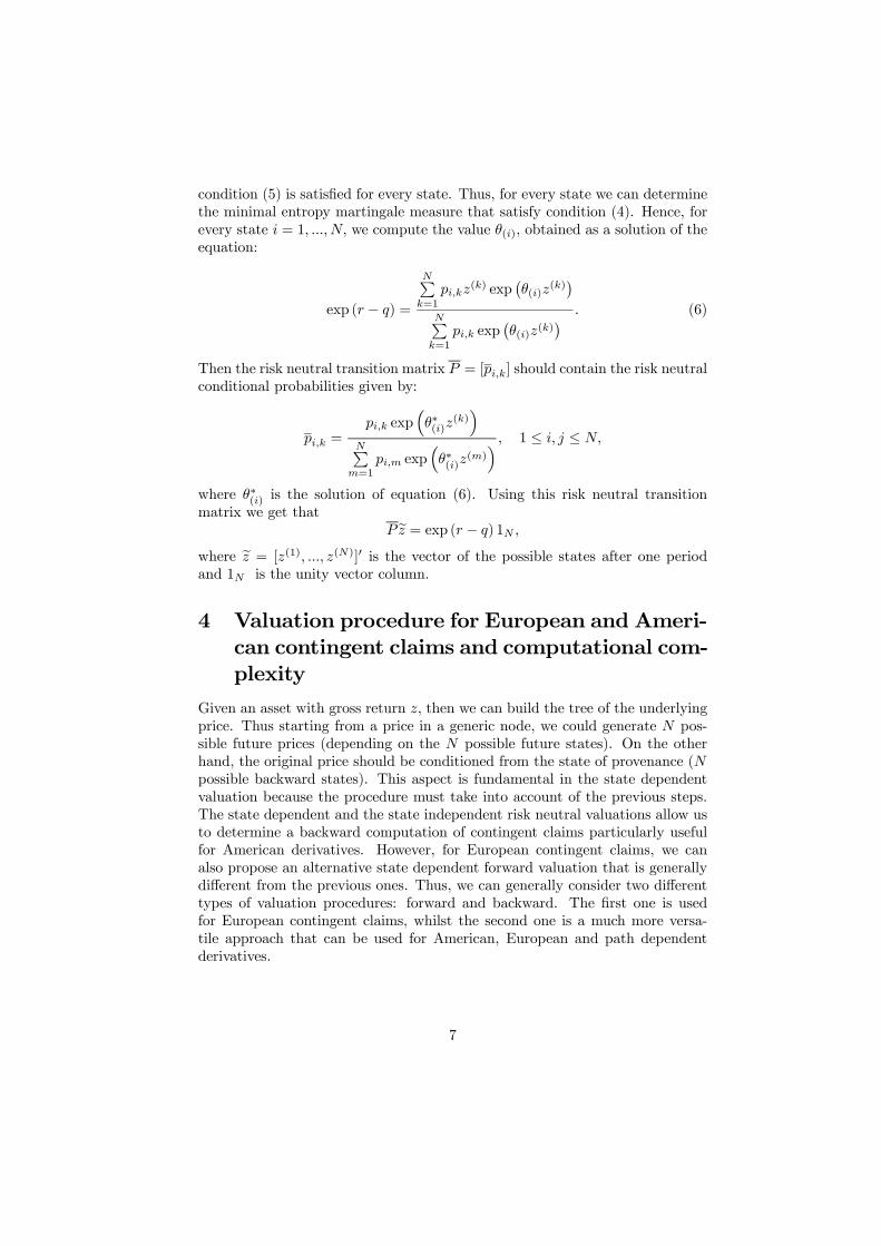
5 Stability of the price valuationFrom the analysis of the backward valuation procedure we understand that thestability of the price depend on the opportune number of states N used in thepricing valuation. From a simple empirical analysis we could observe that theprice of contingent claims do not substantially change with N greater than 50.In particular, we consider historical data from January 1995 to August 2005of Dow Jones Industrials, S&P500 and Nasdaq and we compute the price ofseveral European puts and calls changing the number of the states (from 10 to200) the strikes (five in the money and five out the money) and the time tomaturity (7) for a total of 210 possible options. We compute the prices with astate dependent valuation and with a state independent valuation. While thereexist differences in the prices, we generally do not observe differences in stabilitybetween the two procedures. Moreover, for all the experiments we obtain thestability of the price with N around 40, while, for N lower than 40, we notalways have a stable price.Figure 1 and 2 summarize two of these experiments for a call and a put on

the S&P500. The graphs show clearly how increasing the number of the statesthe prices tend to be stable and it makes sense to consider at least 50 states.On the other hand, the valuation of the price of contingent claims with

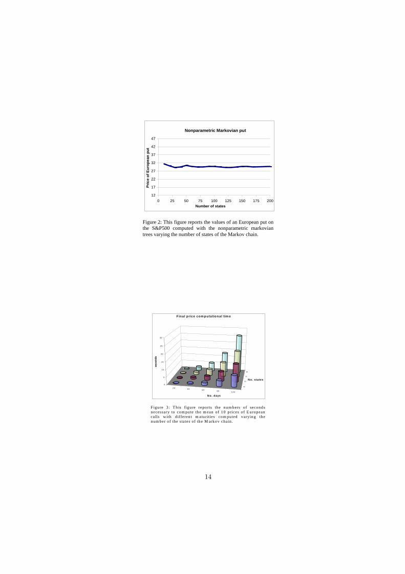
the above algorithms requires few seconds using a notebook dual centrino withone Gb of Ram. As a matter of fact, Figure 3 reports the graphs with theseconds necessary to compute the price of an European call with a backwardstate dependent valuation and considering the mean of 10 prices with maturity20, 40, 60, 90, 120 trading days and states varying between (41-50), (51-60)(61-70) (71-80).In view of this simple empirical analysis, next we consider as contingent

13

Nonparametric Markovian put

12

17

22

27

32

37

42

47

0 25 50 75 100 125 150 175 200Number of states

Pric

e of

Eur

opea

n pu

t

Figure 2: This figure reports the values of an European put on the S&P500 computed with the nonparametric markovian trees varying the number of states of the Markov chain.

20 40 6 0 90 1 20

50

60

70

80

0

5

10

15

20

25

30

seco

nds

N o . d ays

N o . s tates

F ina l price com putational tim e

F igu re 3 : T h is figu re reports the num bers o f seconds necessary to com pute th e m ean of 10 p rices o f E uropean calls w ith d ifferent m aturities com puted varyin g the num ber of the states of th e M arkov chain .

14

claim price, the average of the prices obtained with transition matrixes from 40to 60 states.

6 An empirical comparison

In this section we propose a comparison between nonparametric markovian op-tion prices and the prices obtained under the Black and Scholes assumptions.First of all we compute the differences of valuation when we assume the hypothe-ses of the Black and Scholes model holds. Then we describe the differences ofprices computed using real data.In order to value the performance of our model when we assume the same

hypotheses of the Black and Scholes model, we propose a MonteCarlo simulationcomparison. In particular, we generate 10000 Gaussian scenarios N(0.002,0.03)of log returns. We assume that the risk free rate is 4% and the price of the stocktoday is 50 USD. Then we compute the prices of call options with 20, 40, 60 daysto maturity considering different exercise prices X (X=42, 44, 46, 48, 50, 52,54, 56, 58). For all the options we compute the real Black and Scholes price theBlack and Scholes estimated price, the price estimated with the backward statedependent and state independent valuation. Then we compute the average of thedifferences observed by estimated models and the real Black and Scholes prices.We observe that the estimated Black and Scholes price differs in average of about0.0001 USD from the real one, while both the backward state dependent andstate independent valuation differ in average of about 0.00025 USD. Therefore,this analysis confirms that the nonparametric markovian models well fit theunderline distribution and we do not observe significative differences betweenthe state dependent and state independent valuations. On the other hand,it is well known that log returns are not Gaussian distributed (see Rachev andMittnik (2000)). In an analysis of long time distributions Iaquinta and Ortobelli(2006) have recently shown that the approximation of the long time returndistributions with a nonparametric markovian tree presents much better fitthan that obtained assuming log-normal distributed returns. Therefore weexpect that the prices computed with markovian trees are more precise thanthose obtained with the Black and Scholes model. Using historical data fromJanuary 1995 to August 2005 of Dow Jones Industrials, S&P500 and Nasdaqwe compute some of these differences in Table 1. In particular Table 1 reportsthe values of European calls and puts valued in different weeks between Julyand August 2005. We assume maturity T = 60; exercise price X = E(ST )and risk-free rate equal to the Treasury Bill 3 months. Since we have notobserved significative differences between the backward state dependent andstate independent valuation, in this table we consider only the state dependentone.

As we can observe from the table there exist significative differences betweenthe pricing models much higher that those observed under the Black and Sc-

15

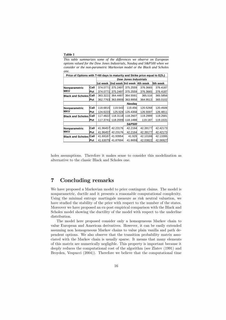
Table 1 This table summarizes some of the differences we observe on European options valued for the Dow Jones Industrials, Nasdaq and S&P500 when we consider or the non-parametric Markovian model or the Black and Scholes one.

Price of Options with T=60 days to maturity and Strike price equal to E(ST) Dow Jones Industrials

1st week 2nd week 3rd week 4th week 5th week Call 374.0771 375.2497 375.2559 376.3665 376.4187 Nonparametric

MKV Put 374.0771 375.2497 375.2559 376.3665 376.4187 Call 363.3221 364.4487 364.5591 365.516 365.5856 Black and Scholes

Put 362.7763 363.8909 363.9958 364.9513 365.0102 Nasdaq

Call 118.6815 119.543 119.456 120.5268 120.4506 Nonparametric MKV Put 124.6223 125.524 125.4358 126.5597 126.4811

Call 117.4822 118.3118 118.2607 119.2999 119.2681 Black and Scholes Put 117.3741 118.2009 118.1488 119.187 119.1531 S&P500

Call 41.96457 42.23176 42.2164 42.39177 42.42173 Nonparametric MKV Put 41.96457 42.23176 42.2164 42.39177 42.42173

Call 41.69187 41.93954 41.929 42.10166 42.13395 Black and Scholes Put 41.63079 41.87694 41.8659 42.03822 42.06927

holes assumptions. Therefore it makes sense to consider this modelization asalternative to the classic Black and Scholes one.

7 Concluding remarksWe have proposed a Markovian model to price contingent claims. The model isnonparametric, ductile and it presents a reasonable computational complexity.Using the minimal entropy martingale measure as risk neutral valuation, wehave studied the stability of the price with respect to the number of the states.Moreover we have proposed an ex-post empirical comparison with the Black andScholes model showing the ductility of the model with respect to the underlinedistribution.The model here proposed consider only a homogeneous Markov chain to

value European and American derivatives. However, it can be easily extendedassuming non homogeneous Markov chains to value plain vanilla and path de-pendent options. We also observe that the transition probability matrix asso-ciated with the Markov chain is usually sparse. It means that many elementsof this matrix are numerically negligible. This property is important because itdeeply reduces the computational cost of the algorithm (see Zlatev (1991) andBroyden, Vespucci (2004)). Therefore we believe that the computational time

16

of O(N3k2) order could be further reduced taking into account this fact.

References[1] Ait-Sahalia Y., Lo A.W. 1998. Nonparametric estimation of state price

densities implicit in financial asset prices, Journal of Finance 53, 499-549.

[2] Ait-Sahalia Y.1996. Nonparametric pricing of interest rate derivative secu-rities, Econometrica 64, 527-560.

[3] Blasi, A., Janssen, J., Manca, R., 2003. Numerical treatment of homoge-neous and non-homogeneous reliability semi-Markov models. Commu-nications in Statistics, Theory and Models.

[4] Broyden, C. G., Vespucci, M. T., 2004. Krylov Solvers for Linear AlgebraicSystems. Elsevier, New York.

[5] D’Amico, G., Janssen, J., Manca, R., June 2005. Non-homogeneous back-ward semi-Markov reliability approach to downward migration creditrisk problem. Proceedings of the 8th Italian Spanish Meeting on Finan-cial Mathematics, Verbania, June 2005.

[6] Duan, J., Dudley, E., Gauthier, G., Simonato, J., 2003. Pricing discretelymonitored barrier options by a Markov chain. Journal of Derivatives 10,9—23.

[7] Duan, J., Simonato, J., 2001. American option pricing under GARCH bya Markov chain approximation. Journal of Economic Dynamics andControl 25, 1689—1718.

[8] Frittelli M., 2000. The minimal entropy martingale measure and the valu-ation problem in incomplete markets, Mathematical Finance 10, 39-52.

[9] Gerber H.U., Shiu, E.S.W., 1994. Option pricing by Esscher transform,Transactions of the Society of Actuaries 46, 99-140; Discussion 141-191.

[10] Gerber H.U., Shiu, E.S.W., 1996. Actuarial bridges to dynamic hedging andoption pricing. Insurance: Mathematics and Economics 18, 183-218.

[11] Hutchinson, J.M., Lo A. W., Poggio T., 1994. A non parametric approachto the pricing and hedging of derivative securities via learning networks,Journal of Finance 49, 851-889.

[12] Iaquinta G. and Ortobelli S., 2006. Distributional Approximation of AssetReturns with Nonparametric Markovian Trees, International Journal ofComputer Science and Network Security, VOL.6 No.10.

[13] Limnios, N., Oprisan, G., 2001. Semi-Markov processes and reliability mod-eling. World Scientific, Singapore.

[14] Rachev, S., Mittnik, S., 2000. Stable Paretian Models in Finance. JohnWiley & Sons, New York.

17

[15] Schoutens W. 2003. Lèvy Processes in Finance: Pricing Financial Deriva-tives, Chichester, John Wiley & Sons.

[16] Stutzer, M. J. 1996. A Simple Nonparametric Approach to Derivative Se-curity Valuation, Journal of Finance 51, 1633-1652.

[17] Zlatev, Z., 1991. Computational Methods for General Sparse Matrices.Kluwer, Boston.

18

Redazione Dipartimento di Matematica, Statistica, Informatica ed Applicazioni Università degli Studi di Bergamo Via dei Caniana, 2 24127 Bergamo Tel. 0039-035-2052536 Fax 0039-035-2052549 La Redazione ottempera agli obblighi previsti dall’art. 1 del D.L.L. 31.8.1945, n. 660 e successive modifiche

Stampato nel 2006 presso la Cooperativa

Studium Bergomense a r.l. di Bergamo