METRON - International Journal of Statistics2006, vol. LXIV, n. 1, pp. 47-60

AYMAN BAKLIZI – OMAR EIDOUS

Nonparametric estimation of P(X < Y)using kernel methods

Summary - In this paper we consider point and interval estimation of P(X < Y ).We used the kernel density estimators of the densities of the random variables Xand Y , assumed independent. The resulting statistic is found to be similar in manyways to the Mann-Whitney statistic, however it assigns smooth continuous scores tothe pairs of the observations rather than the zero or one scores of the Mann-Whitneystatistic. A simulation study is conducted to investigate and compare the performanceof the estimator based on this statistic and the Mann-Whitney estimator. Bootstrapconfidence intervals based on the two statistics are investigated and compared.

Key Words - Bootstrap intervals; Kernel density estimator; Mann-Whitney statistic;Stress-strength.

1. Introduction

A wide range of problems in engineering and medicine, as well as someother fields involve inference about the quantity p = P(X < Y ) where X andY may denote the stress and the strength variables in the context of mechanicalreliability of a system. The system fails any time its strength is exceeded bythe stress applied to it. In a medical setting, P(X < Y ) measures the effect ofthe treatment when X is the response for a control group and Y refers to thetreatment group.

Several authors have considered statistical inference about P(X < Y ) undera parametric setup, see for example Reiser and Guttman (1986), Johnson etal. (1994) and the references therein. When there is not enough evidence fora specific parametric model for the distribution generating the data, one mayconsider nonparametric methods. There are several authors who discuss pointand interval estimation in the nonparametric case (Sen, 1967; Govindarajulu,1968 and 1976; Halperin et al., 1987 and Hamdy, 1995), see Kotz et al. (2003)as a general reference. Let X1, . . . , Xn1 and Y1, . . . , Yn1 be two independent

Received December 2004 and revised September 2005.

48 AYMAN BAKLIZI – OMAR EIDOUS

random samples from the distributions of X and Y respectively. The Mann-Whitney statistic (Lehmann, 1975) is defined as W = ∑n1

i=1∑n2

j=1 φ(Xi , Yj )

where φ(Xi , Yj ) = 1 if Xi < Yj and 0 otherwise. A version correctedfor ties is also given in Lehmann (1975). It is readily seen that E(W ) =E(∑n1

i=1∑n2

j=1 φ(Xi , Yj )

)= n1n2 P(X < Y ), therefore an unbiased estimator

for p is given by p1 = 1n1n2

∑n1i=1

∑n2j=1 φ(Xi , Yj ). In fact, p1 is the uniformly

minimum variance unbiased estimator for p. The variance of p1 is given by

var( p1) = 1

n1n2[(n1−1)

∫F2

1 d F2+(n2−1)

∫F2

2 d F1−(n2−1)+(2n2−1)p−(n1+n2−1)p2

]

where F1 and F2 are the distribution functions of X and Y respectively. Sev-eral authors have considered the problem of constructing distribution-free con-fidence intervals for p using this unbiased estimator. Sen (1967) showed that√

n0( p1 − p) is asymptotically normally distributed where n0 = n1n2n1+n2

. He alsoprovided a consistent estimator for the asymptotic variance of

√n0( p1 − p)

which can be used to construct approximate confidence intervals. Govindara-julu (1968) showed that

√min(n1, n2)( p1 − p)/SG is asymptotically normal

where S2G is an unbiased, distribution-free and consistent estimator of the vari-

ance of√

min(n1, n2)( p1 − p)/SG . Halperin et al. (1987) have shown that√min(n1, n2)( p1 − p)/νH is asymptotically normal where

νH = p(1 − p)(

n1

∫F2

n1dGn2 +n2

∫G2

n2d Fn1 −n2+(2n2−1) p1−(n1+n2−2) p2

1

)p1(1 − p1)

+ 1

.

They use this result to construct distribution free intervals for p.Hamdy (1995), using the approach of Halperin et al. (1987), has constructed

the pivotal quantity with an asymptotic chi-squared distribution with one degreeof freedom, which can be used to construct confidence intervals for p. Thispivotal quantity is given by

Z 2(p) = ( p1 − p)2/(θ(AL − AU ) + AU )

Nonparametric estimation of P(X<Y) using kernel methods 49

where θ is obtained by substituting p1 in place of p in the expression

θ = 1

AL − AU(K − (n2 − 1) + (2n2 − υ − 1)p − (µ − 1)p2)

AL − AU =

1

µν

(4

3r√

2(µ − 1)(ν − 1)r − (ν − 1)r)

if(µ − 1)

(v − 1)≥ 2r

1

µν

((µ − nu)r(1 − r) − (µ − 1)2

12(ν − 1)

)if

(µ − 1)

(v − 1)< 2r

AU = νr(1 − r)/(µν), r = min(p, 1 − p),

µ = min(n1, n2), ν = max(n1, n2) and

K = (n1 − 1)

∫F2dG + (n2 − 1)

∫G2d f

which can be estimated consistently as in Hamdy (1995).In this paper we develop a new estimator for P(X < Y ) using kernel

methods. The estimator of p is introduced in Section 2. Confidence intervalsbased on the proposed statistic as well as the Mann-Whitney Statistic are givenin Section 3. A simulation study is conducted in Section 4 to evaluate theperformance of the estimators and intervals. The results and conclusions aregiven in the final section.

2. The kernel – based estimator

Let X1, X2, . . . , Xn1 and Y1, Y2, . . . , Yn2 be two independent random sam-ples from an unknown probability density functions fX and fY respectively.The parameter p we want to estimate is

p = P(X < Y ) =∫ ∞

−∞

∫ y

−∞fX (x) fY (y)dx dy . (1)

The kernel density estimators of fX and fY when the two random variables Xand Y are defined on the entire real line are given by

f X (x) = 1

n1h1

n1∑i=1

K(

x − Xi

h1

), − ∞ < x < ∞ (2)

fY (y) = 1

n2h2

n2∑j=1

K(

y − Yi

h2

), − ∞ < x < ∞ (3)

where h1 and h2 are positive numbers which control the smoothness of thefitted curves for X and Y respectively, usually called bandwidths or smoothing

50 AYMAN BAKLIZI – OMAR EIDOUS

parameters. K (u) is a kernel function which is a symmetric probability density.Reviews of kernel methods are available in Silverman (1986) and Wand andJones (1995). The proposed estimator for p is

p2 =∫ ∞

−∞

∫ y

−∞f X (x) fY (y)dx dy .

It can be easily seen that

p2 =∫∫ ∫∫

I [x + h1ν < y + h2w]K (ν)K (w)dν dw d F(x)dG(y)

=∫∫ ∫∫

I [h1ν − h2w < y − x]K (ν)K (w)dν dw d F(x)dG(y)

=∫∫

H(y − x)d F(x)dG(y)

where H is the distribution function of h1V −h2W with V and W independentrandom variables with common density K and I [·] is the usual indicator func-tion. If K is the standard normal density then H is the distribution function of

a normal random variable with mean 0 and standard deviation t =√

h21 + h2

2.In this case, p2 becomes the two sample U -statistic

p2 = 1

n1n2

n1∑i=1

n2∑j=1

�((Yj − Xi)/t)

where � is the standard normal distribution function.

3. Bootstrap intervals

Let p be either the Mann-Whitney or the kernel based estimator of pcalculated from the original two samples. Let p∗ be the corresponding esti-mator calculated from the bootstrap samples. Now we simulate the bootstrapdistribution of p by re-sampling independently from the empirical distributionsof X and Y based on the original data (Davison and Hinkley, 1997, pp. 71)and calculating p∗

i , i = 1, . . . , B where B is the number of bootstrap samples.Let H ∗ be the cumulative distribution function of p∗, then the 1 − α intervalis given by

(H ∗−1

(α2

), H ∗−1

(1 − α

2

)). This is called the percentile interval.

The bias corrected and accelerated (BCa) interval is calculated also usingthe percentiles of the bootstrap distribution of p∗. The percentiles depend ontwo numbers α and z0 called the acceleration and the bias correction. The1 − α interval (BCa) is given by(

H ∗−1(α1), H ∗−1(α2))

Nonparametric estimation of P(X<Y) using kernel methods 51

where

α1 = �

(z0 + z0 + zα/2

1 − α(z0 + zα/2)

), α2 = �

(z0 + z0 + z1−α/2

1 − α(z0 + z1−α/2)

),

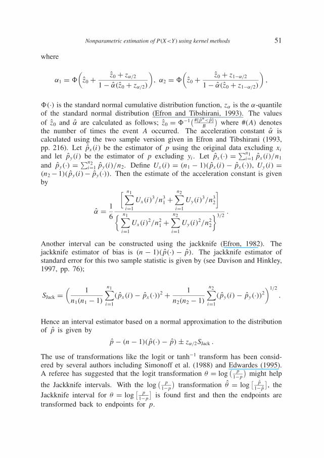
�(·) is the standard normal cumulative distribution function, zα is the α-quantileof the standard normal distribution (Efron and Tibshirani, 1993). The valuesof z0 and α are calculated as follows; z0 = �−1

( #{ p∗< p}B

)where #(A) denotes

the number of times the event A occurred. The acceleration constant α iscalculated using the two sample version given in Efron and Tibshirani (1993,pp. 216). Let px(i) be the estimator of p using the original data excluding xi

and let py(i) be the estimator of p excluding yi . Let px(·) = ∑n1i=1 px(i)/n1

and py(·) = ∑n2i=1 py(i)/n2. Define Ux(i) = (n1 − 1)( px(i) − px(·)), Uy(i) =

(n2 − 1)( py(i)− py(·)). Then the estimate of the acceleration constant is givenby

α = 1

6

[ n1∑i=1

Ux(i)3/n3

1 +n2∑

i=1

Uy(i)3/n3

2

]{ n1∑

i=1

Ux(i)2/n2

1 +n2∑

i=1

Uy(i)2/n2

2

}3/2.

Another interval can be constructed using the jackknife (Efron, 1982). Thejackknife estimator of bias is (n − 1)( p(·) − p). The jackknife estimator ofstandard error for this two sample statistic is given by (see Davison and Hinkley,1997, pp. 76);

SJack =(

1

n1(n1 − 1)

n1∑i=1

( px(i) − px(·))2 + 1

n2(n2 − 1)

n2∑i=1

( py(i) − py(·))2)1/2

.

Hence an interval estimator based on a normal approximation to the distributionof p is given by

p − (n − 1)( p(·) − p) ± zα/2SJack .

The use of transformations like the logit or tanh−1 transform has been consid-ered by several authors including Simonoff et al. (1988) and Edwardes (1995).A referee has suggested that the logit transformation θ = log

( p1−p

)might help

the Jackknife intervals. With the log( p

1−p

)transformation θ = log

[ p1− p

], the

Jackknife interval for θ = log[ p

1−p

]is found first and then the endpoints are

transformed back to endpoints for p.

52 AYMAN BAKLIZI – OMAR EIDOUS

4. Small sample performance of the estimators

In our simulations we used the estimator based on the normal kernel

p2 = 1

n1n2

n1∑i=1

n2∑j=1

�((Yj − Xi)/t)

with t =√

h21 + h2

2. The bandwidths are chosen as in Silverman (1986, p. 57-58). The performances of the Mann-Whitney estimator and the proposed es-timator were investigated and compared by their mean squared error. Therelative efficiency of the proposed estimator to the Mann-Whitney estimatorare calculated as the ratio of mean squared errors.

A simulation study is conducted to investigate the performance of the pointestimators. The indices of our simulations are:

(n1, n2) = (5,5), (10,10), (20,20), (30,30), (50,50), (100,100)

p: the true value of P(X < Y ) and is taken to be 0.02, 0.05, 0.1, 0.3, 0.5.By symmetry, results for values of p = 0.7, 0.9, 0.95, 0.98 are similar to

those of p = 0.3, 0.1, 0.05, 0.02 respectively.We considered the following cases for the parent distributions from which

the data are generated:1) X and Y have exponential distributions with means 1 and λ respectively.

The value of λ is chosen such that we get the values of p determinedabove. Since p = λ

λ+1 we get λ = p1−p .

2) X ∼ N (µ1, σ21 ), Y ∼ N (µ2, σ

22 ) where µ1 = 0, σ 2

1 = 1, σ 22 = 1, 2, 4 and

µ2 = (1 + σ 22 )1/2�−1(p).

For each combination of n1, n2, parent distribution and p, 1000 samples weregenerated for X and 1000 samples for Y independently. The estimators arecalculated, the bias of our estimator, the variances and efficiencies are obtained.

For the confidence intervals with nominal confidence coefficient (1 − α),we take α = 0.05 and use the criterion of attainment of lower and upper errorprobabilities which are both equal to α

2 .A simulation study was also conducted to investigate the performance of

the intervals. The indices of our simulations were:

(n1, n2) = (25,25), (40,40), (25,40), (40,25)

p: the true value of P(X < Y ) and is taken to be 0.02, 0.05, 0.1, 0.3, 0.5.For each combination of n1, n2, and parent distribution, 1000 samples

were generated for X and 1000 samples for Y independently. The intervalswith nominal error probability α = 0.05 are calculated, and we used B = 500replications for bootstrap calculations. The following quantities are simulatedfor each interval using the results of the 1000 samples:

Nonparametric estimation of P(X<Y) using kernel methods 53

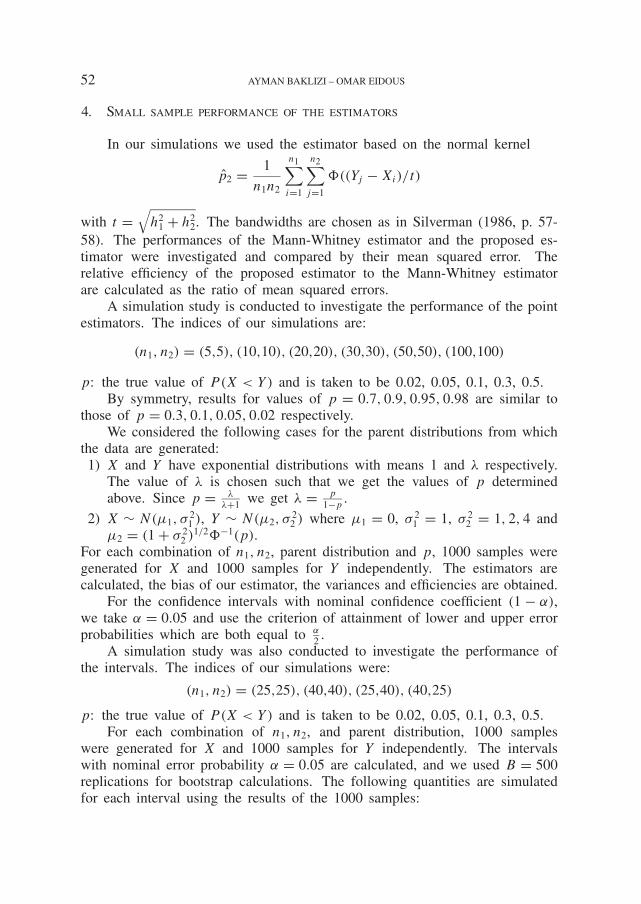
– Lower error rates (L): the fraction of intervals where the lower bound exceedsthe true parameter.– Upper error rates (U): the fraction of intervals where the upper bound liesbelow the true parameter.– Total error rates (T): the fraction of intervals that did not contain the trueparameter value.In Table 2 we used the following abbreviations for the intervals under study:

PERC1: percentile intervals based on the Mann-Whitney statistic.PERC2: percentile intervals based on the kernel statistic.

BCa1: Bias corrected and accelerated intervals based on the Mann-Whitneystatistic.

BCa2: Bias corrected and accelerated intervals based on the kernel statistic.JKNF1: jackknife intervals based on the Mann-Whitney statistic.JKNF2: jackknife intervals based on the kernel statistic.

TRJKNF1: transformed jackknife intervals based on the Mann-Whitney statistic.TRJKNF2: transformed jackknife intervals based on the kernel statistic.

AS: the asymptotic interval of Hamdy (1995) based on the Mann-Whitneystatistic.

5. Results and conclusions

Results concerning the bias of the proposed estimator, the variances of theestimators and their relative efficiency are presented in Table 1. It appears thatour estimator is slightly positively biased for values of p near zero or one. Thebias decreases as p gets closer to 0.5. The results about the relative efficiencyof our estimator to the Mann-Whitney estimator show that our estimator isbetter than the Mann-Whitney estimator for values of p close to 0.5. Theyhave about similar performance for symmetric distributions. Otherwise, forskewed distributions the Mann-Whitney statistic dominates, especially for verysmall or large values of p. However, the performance of the kernel estimatormay be improved when using more sophisticated types of kernels, bandwidthselection rules, and bias corrections.

For the interval estimation procedures, the results are given in Table 2. Itappears that BCa2, Jknf2 and TRJknf2 intervals tend to have the best overallperformance among those considered. However their performance and the per-formance of the other re-sampling intervals is very bad when p is very small(p = 0.02) as they tend to be rather anti-conservative and highly asymmet-ric. The best interval in this situation is the asymptotic interval, however it isalso highly asymmetric. In most cases, the performance of intervals based onthe kernel estimator tends to be better than that based on the Mann-Whitneystatistic, they are often more symmetric and tend to be closer to the nominallevels. The results show that intervals based on the asymptotic distribution

54 AYMAN BAKLIZI – OMAR EIDOUS

are anti-conservative and highly asymmetric, however for very small or verylarge values of p, they appear to be better than re-sampling based intervals.The logit transformation appears to improve on the performance of Jackknifeintervals. It may be a good idea for future research to find the transformationthat “best” improves the performance of the intervals. Also, as suggested by areferee, the use of a continuity correction with the suitable transformation mayfurther improve the performance of the intervals.

In conclusion it appears that the kernel procedure with the bootstrap orJackknife are effective for the interval estimation problem, the logit transforma-tion improves the performance of the Jackknife procedures, and in most casesthe performance of kernel based intervals is better than intervals based on theMann-Whitney statistic.

Table 1: Biases, variances and the relative efficiency of the estimators

n p Bias ( p2) Var ( p1) Var ( p2) eff n p Bias ( p2) Var ( p1) Var ( p2)

Exponential Exponential

5 0.02 0.0654 0.0022 0.0087 0.2516 30 0.02 0.0425 0.0003 0.0025 0.13745 0.05 0.0579 0.0066 0.0097 0.6824 30 0.05 0.0339 0.0009 0.0021 0.45555 0.10 0.0402 0.0131 0.0110 1.1903 30 0.10 0.0201 0.0019 0.0021 0.93705 0.30 0.0098 0.0286 0.0230 1.2453 30 0.30 0.0015 0.0045 0.0041 1.09515 0.50 0.0025 0.0364 0.0314 1.1594 30 0.50 −0.0004 0.0056 0.0053 1.0553

Normal (σ 22 = 1) Normal (σ 2

2 = 1)

5 0.02 0.0062 0.0017 0.0019 0.9322 30 0.02 0.0020 0.0002 0.0002 0.93805 0.05 0.0075 0.0050 0.0046 1.0843 30 0.05 0.0021 0.0007 0.0007 0.96735 0.10 0.0035 0.0098 0.0091 1.0760 30 0.10 0.0025 0.0015 0.0015 0.99065 0.30 0.0025 0.0307 0.0278 1.1055 30 0.30 0.0007 0.0045 0.0044 1.03765 0.50 −0.0012 0.0361 0.0325 1.1112 30 0.50 0.0008 0.0058 0.0056 1.0388

Normal (σ 22 = 2) Normal (σ 2

2 = 2)

5 0.02 0.0038 0.0019 0.0018 1.0511 30 0.02 0.0015 0.0002 0.0002 0.95665 0.05 0.0098 0.0059 0.0058 1.0130 30 0.05 0.0025 0.0008 0.0008 0.95705 0.10 0.0131 0.0123 0.0113 1.0896 30 0.10 0.0048 0.0015 0.0016 0.97515 0.30 0.0102 0.0311 0.0284 1.0963 30 0.30 0.0031 0.0047 0.0045 1.03685 0.50 0.0088 0.0355 0.0318 1.1153 30 0.50 0.0007 0.0059 0.0057 1.0476

Normal (σ 22 = 4) Normal (σ 2

2 = 4)

5 0.02 0.0076 0.0024 0.0022 1.0830 30 0.02 0.0019 0.0003 0.0003 0.96355 0.05 0.0034 0.0053 0.0050 1.0670 30 0.05 0.0040 0.0009 0.0009 0.96685 0.10 0.0121 0.0114 0.0106 1.0788 30 0.10 0.0031 0.0017 0.0017 0.99875 0.30 0.0110 0.0302 0.0272 1.1103 30 0.30 0.0034 0.0050 0.0048 1.04385 0.50 −0.0012 0.0384 0.0336 1.1418 30 0.50 0.0001 0.0060 0.0057 1.0508

Exponential Exponential

10 0.02 0.0567 0.0011 0.0052 0.2070 50 0.02 0.0361 0.0002 0.0016 0.126110 0.05 0.0450 0.0027 0.0049 0.5455 50 0.05 0.0270 0.0005 0.0013 0.415310 0.10 0.0341 0.0056 0.0055 1.0134 50 0.10 0.0167 0.0011 0.0013 0.884010 0.30 0.0108 0.0149 0.0128 1.1614 50 0.30 0.0051 0.0028 0.0026 1.080110 0.50 −0.0081 0.0176 0.0156 1.1301 50 0.50 0.0026 0.0034 0.0032 1.0506

Nonparametric estimation of P(X<Y) using kernel methods 55

Table 1: Continuedn p Bias ( p2) Var ( p1) Var ( p2) eff n p Bias ( p2) Var ( p1) Var ( p2)

Normal (σ 22 = 1) Normal (σ 2

2 = 1)

10 0.02 0.0028 0.0007 0.0007 0.9515 50 0.02 0.0019 0.0001 0.0001 0.928010 0.05 0.0046 0.0022 0.0023 0.9723 50 0.05 0.0029 0.0004 0.0004 0.950310 0.10 0.0032 0.0050 0.0050 1.0018 50 0.10 0.0052 0.0009 0.0010 0.971210 0.30 0.0047 0.0140 0.0129 1.0837 50 0.30 0.0025 0.0028 0.0027 1.021510 0.50 −0.0027 0.0180 0.0166 1.0839 50 0.50 0.0019 0.0033 0.0032 1.0347

Normal (σ 22 = 2) Normal (σ 2

2 = 2)

10 0.02 0.0025 0.0008 0.0008 0.9889 50 0.02 0.0015 0.0001 0.0002 0.947410 0.05 0.0061 0.0025 0.0025 0.9778 50 0.05 0.0021 0.0004 0.0004 0.965010 0.10 0.0054 0.0051 0.0051 1.0018 50 0.10 0.0031 0.0010 0.0010 986010 0.30 0.0060 0.0142 0.0133 1.0679 50 0.30 0.0045 0.0029 0.0028 1.021410 0.50 −0.0004 0.0184 0.0171 1.0734 50 0.50 −0.0019 0.0033 0.0031 1.0423

Normal (σ 22 = 4) Normal (σ 2

2 = 4)

10 0.02 0.0036 0.0010 0.0011 0.9428 50 0.02 0.0018 0.0002 0.0002 0.947110 0.05 0.0040 0.0025 0.0025 0.9809 50 0.05 0.0010 0.0005 0.0005 0.979410 0.10 0.0070 0.0061 0.0059 1.0286 50 0.10 0.0028 0.0011 0.0011 0.991410 0.30 0.0049 0.0164 0.0152 1.0780 50 0.30 0.0007 0.0029 0.0028 1.036910 0.50 −0.0011 0.0177 0.0164 1.0786 50 0.50 0.0009 0.0034 0.0033 1.0402

Exponential Exponential

20 0.02 0.0481 0.0005 0.0032 0.1485 100 0.02 0.0285 0.0001 0.0010 0.114620 0.05 0.0375 0.0013 0.0026 0.4906 100 0.05 0.0192 0.0003 0.0006 0.417920 0.10 0.0242 0.0026 0.0028 0.9316 100 0.10 0.0125 0.0005 0.0006 0.831120 0.30 0.0009 0.0064 0.0056 1.1374 100 0.30 0.0025 0.0013 0.0012 1.050520 0.50 −0.0001 0.0085 0.0079 1.0848 100 0.50 0.0001 0.0015 0.0015 1.0379

Normal (σ 22 = 1) Normal (σ 2

2 = 1)

20 0.02 0.0021 0.0003 0.0003 0.9163 100 0.02 0.0013 0.0001 0.0001 0.936020 0.05 0.0043 0.0011 0.0012 0.9461 100 0.05 0.0020 0.0002 0.0002 0.960920 0.10 0.0082 0.0024 0.0025 0.9785 100 0.10 0.0024 0.0004 0.0005 0.976620 0.30 0.0037 0.0069 0.0066 1.0446 100 0.30 0.0020 0.0013 0.0013 1.015620 0.50 −0.0028 0.0091 0.0086 1.0573 100 0.50 −0.0002 0.0016 0.0016 1.0254

Normal (σ 22 = 2) Normal (σ 2

2 = 2)

20 0.02 0.0019 0.0004 0.0004 0.9489 100 0.02 0.0012 0.0001 0.0001 0.948820 0.05 0.0047 0.0011 0.0011 0.9684 100 0.05 0.0013 0.0002 0.0002 0.976020 0.10 0.0058 0.0027 0.0027 0.9873 100 0.10 0.0039 0.0005 0.0005 0.967420 0.30 0.0056 0.0069 0.0066 1.0443 100 0.30 0.0026 0.0014 0.0014 1.011120 0.50 −0.0022 0.0089 0.0084 1.0588 100 0.50 0.0013 0.0017 0.0016 1.0248

Normal (σ 22 = 4) Normal (σ 2

2 = 4)

20 0.02 0.0022 0.0005 0.0005 0.9518 100 0.02 0.0010 0.0001 0.0001 0.974520 0.05 0.0049 0.0013 0.0014 0.9787 100 0.05 0.0020 0.0002 0.0002 0.972920 0.10 0.0068 0.0028 0.0028 1.0046 100 0.10 0.0024 0.0005 0.0005 0.985320 0.30 0.0058 0.0077 0.0074 1.0489 100 0.30 −0.0004 0.0015 0.0015 1.022820 0.50 0.0026 0.0082 0.0077 1.0744 100 0.50 −0.0009 0.0019 0.0018 1.0275

56 AYMAN BAKLIZI – OMAR EIDOUS

Table 2 (a): Error probabilities of the intervals (Exponential parent distribution)

L U T L U T L U T L U T

p (n1, n2) = (25, 25) (40, 40) (25, 40) (40, 25)

0.02 PERC1 009 467 476 095 180 275 031 411 442 043 281 324PERC2 000 796 796 000 726 726 000 787 787 000 761 761BCa1 000 482 482 037 192 229 003 425 428 007 296 303BCa2 000 907 907 000 847 847 000 908 908 000 872 872

JKNF1 036 465 501 133 177 310 053 410 463 078 278 356JKNF2 000 722 722 000 621 621 000 684 684 000 668 668

TRJknf1 000 483 483 000 195 195 000 432 432 000 296 296TRJknf2 000 910 910 000 85 853 000 910 910 000 874 874

AS 000 514 514 000 226 226 000 461 461 000 323 323

0.05 PERC1 082 109 191 107 015 122 110 064 174 090 024 114PERC2 000 231 231 003 172 175 006 205 211 002 180 182BCa1 026 122 148 048 029 077 060 077 137 038 032 070BCa2 000 311 311 001 267 268 002 292 294 000 252 252

JKNF1 117 104 221 128 012 140 142 059 201 126 018 144JKNF2 000 184 184 004 128 132 006 167 173 004 135 139

TRJknf1 000 122 122 015 028 043 003 082 085 000 038 038TRJknf2 000 331 331 000 292 292 002 322 324 000 285 285

AS 000 145 145 028 053 081 033 107 140 010 060 070

0.1 PERC1 087 016 103 087 007 094 096 006 102 071 009 080PERC2 028 059 087 027 052 079 031 043 074 035 041 076BCa1 033 028 061 046 016 062 053 010 063 032 021 053BCa2 012 078 090 010 075 085 014 054 068 014 075 089

JKNF1 115 010 125 106 002 108 110 003 113 096 004 100JKNF2 034 033 067 034 032 066 039 026 065 036 023 059

TRJknf1 007 036 043 024 021 045 028 014 042 016 022 038TRJknf2 003 085 088 005 081 086 007 070 077 005 079 084

AS 019 053 072 023 037 060 039 025 064 016 039 055

0.3 PERC1 040 014 054 041 020 061 049 019 068 031 019 050PERC2 032 024 056 036 028 064 036 023 059 031 024 055BCa1 021 026 047 032 020 052 024 022 046 020 024 044BCa2 016 029 045 027 031 058 020 024 044 020 029 049

JKNF1 049 012 061 045 020 065 048 019 067 041 016 057JKNF2 042 019 061 040 023 063 045 021 066 031 019 050

TRJknf1 013 020 033 024 024 048 020 024 044 016 022 038TRJknf2 010 02 036 022 028 050 018 027 045 013 030 043

AS 018 032 050 024 030 054 024 030 054 018 033 051

0.5 PERC1 030 029 059 026 018 044 033 027 060 026 017 043PERC2 031 029 060 022 023 045 034 027 061 029 018 047BCa1 025 025 050 023 015 038 027 019 046 022 013 035BCa2 025 025 050 024 018 042 029 019 048 025 014 039

JKNF1 035 033 068 025 020 045 033 028 061 029 023 052JKNF2 033 035 068 024 024 048 034 032 066 029 020 049

TRJknf1 023 028 051 021 016 037 024 022 046 023 016 039TRJknf2 024 026 050 023 017 040 027 024 051 024 017 041

AS 028 031 059 023 018 041 032 028 060 028 021 049

Nonparametric estimation of P(X<Y) using kernel methods 57

Table 2 (b): Error probabilities of the intervals (Normal parent distribution, σ 22 = 1)

L U T L U T L U T L U T

p (n1, n2) = (25, 25) (40, 40) (25, 40) (40, 25)

0.02 PERC1 016 252 268 080 043 123 040 132 172 038 131 169PERC2 009 255 264 069 045 114 034 135 169 032 137 169BCa1 000 265 265 024 055 079 007 150 157 001 148 149BCa2 000 270 270 028 064 092 007 163 170 003 159 162

JKNF1 046 246 292 131 039 170 080 129 209 083 127 210JKNF2 027 247 274 101 039 140 054 129 183 059 127 186

TRJknf1 000 266 266 000 052 052 000 151 151 000 150 150TRJknf2 000 272 272 001 060 061 000 161 161 000 164 164

AS 000 301 301 000 087 087 000 192 192 000 190 190

0.05 PERC1 076 045 121 082 013 095 095 018 113 082 012 094PERC2 065 051 116 071 020 091 086 024 110 072 014 086BCa1 017 067 084 039 022 061 045 034 079 032 015 047BCa2 021 079 100 040 030 070 045 044 089 037 021 058

JKNF1 115 037 152 109 004 113 127 016 143 117 010 127JKNF2 090 041 131 086 007 093 103 018 121 095 010 105

TRJknf1 000 066 066 008 026 034 000 035 035 000 017 017TRJknf2 001 075 076 015 033 048 013 043 056 008 022 030

AS 000 100 100 017 049 066 008 057 065 004 039 043

0.1 PERC1 075 005 080 049 014 063 062 008 070 064 011 075PERC2 073 016 089 044 017 061 054 012 066 052 016 068BCa1 040 022 062 025 018 043 026 015 041 023 019 042BCa2 041 027 068 020 028 048 024 020 044 023 024 047

JKNF1 105 004 109 066 007 073 086 002 088 090 005 095JKNF2 097 004 101 056 011 067 071 007 078 068 008 076

TRJknf1 005 021 026 014 024 038 012 020 032 009 021 030TRJknf2 013 028 041 010 034 044 013 029 042 010 024 034

AS 010 035 045 014 044 058 016 030 046 012 033 045

0.3 PERC1 032 019 051 037 022 059 038 021 059 041 021 062PERC2 032 021 053 034 026 060 033 024 057 041 023 064BCa1 017 023 040 025 024 049 020 025 045 027 024 051BCa2 018 025 043 023 032 055 023 026 049 026 027 053

JKNF1 039 019 058 039 022 061 048 020 068 045 018 063JKNF2 035 020 055 037 024 061 043 024 067 046 021 067

TRJknf1 008 023 031 017 027 044 013 026 039 016 024 040TRJknf2 010 024 034 018 034 052 012 029 041 017 024 041

AS 013 030 043 018 037 055 012 031 043 020 031 051

0.5 PERC1 031 029 060 025 025 050 032 026 058 01 028 046PERC2 032 027 059 026 029 055 034 028 062 021 028 049BCa1 023 021 044 020 024 044 030 024 054 016 021 037BCa2 026 018 044 020 021 041 034 024 058 016 026 042

JKNF1 031 032 063 023 032 055 034 031 065 016 027 043JKNF2 030 030 060 023 031 054 036 028 064 016 027 043

TRJknf1 018 024 042 021 023 044 029 023 052 011 024 035TRJknf2 022 022 044 020 024 044 031 025 056 013 022 035

AS 023 029 052 021 027 048 034 029 063 016 026 042

58 AYMAN BAKLIZI – OMAR EIDOUS

Table 2 (c): Error probabilities of the intervals (Normal parent distribution, σ 22 = 2)

L U T L U T L U T L U T

p (n1, n2) = (25, 25) (40, 40) (25, 40) (40, 25)

0.02 PERC1 015 280 295 098 081 179 040 139 179 038 188 226PERC2 006 283 289 078 083 161 029 144 173 030 192 222BCa1 000 298 298 023 095 118 004 154 158 005 200 205BCa2 000 306 306 025 107 132 005 168 173 003 208 211

JKNF1 051 278 329 144 078 222 076 137 213 082 186 268JKNF2 024 278 302 112 078 190 061 139 200 049 187 236

TRJknf1 000 294 294 000 098 098 000 153 153 000 203 203TRJknf2 000 303 303 000 104 104 000 166 166 000 208 208

AS 000 331 331 000 121 121 000 196 196 000 226 226

0.05 PERC1 085 050 135 073 011 084 110 014 124 099 019 118PERC2 070 058 128 066 013 079 094 020 114 091 025 116BCa1 019 064 083 032 020 052 037 028 065 045 028 073BCa2 023 078 101 031 039 070 041 039 080 040 037 077

JKNF1 121 045 166 100 003 103 141 012 153 133 016 149JKNF2 097 046 143 084 007 091 121 013 134 120 016 136

TRJknf1 000 067 067 011 025 036 000 030 030 000 035 035TRJknf2 003 081 084 016 038 054 007 036 043 005 041 046

AS 000 094 094 017 047 064 002 060 062 008 049 057

0.1 PERC1 062 008 070 059 011 070 071 015 086 079 008 087PERC2 050 011 061 052 017 069 066 019 085 063 013 076BCa1 025 017 042 020 025 045 031 023 054 035 019 054BCa2 024 024 048 021 030 051 032 029 061 032 025 057

JKNF1 084 006 090 073 007 080 104 006 110 104 005 109JKNF2 070 008 078 067 011 078 085 010 095 090 009 099

TRJknf1 006 026 032 010 020 030 011 025 036 014 022 036TRJknf2 006 034 040 009 030 039 015 036 051 016 028 044

AS 006 047 053 012 039 051 019 044 063 016 034 050

0.3 PERC1 045 017 062 043 021 064 043 024 067 041 022 063PERC2 043 016 059 044 025 069 045 030 075 040 024 064BCa1 029 016 045 030 024 054 028 026 054 024 022 046BCa2 032 016 048 028 025 053 027 029 056 026 024 050

JKNF1 048 013 061 050 018 068 048 024 072 041 017 058JKNF2 047 017 064 046 019 065 051 027 078 038 018 056

TRJknf1 020 019 039 027 026 053 020 031 051 015 028 043TRJknf2 019 022 041 026 025 051 019 038 057 014 030 044

AS 026 032 058 029 033 062 026 043 069 020 036 056

0.5 PERC1 028 024 052 030 026 056 031 030 061 027 026 053PERC2 030 025 055 029 029 058 031 030 061 030 025 055BCa1 021 021 042 023 019 042 024 026 050 023 023 046BCa2 024 022 046 023 021 044 022 029 051 026 024 050

JKNF1 029 027 056 025 027 052 029 033 062 026 030 056JKNF2 030 028 058 025 029 054 030 033 063 027 028 055

TRJknf1 018 021 039 019 023 042 023 026 049 022 020 042TRJknf2 019 022 041 020 025 045 023 030 053 021 022 043

AS 026 024 050 023 026 049 027 032 059 024 027 051

Nonparametric estimation of P(X<Y) using kernel methods 59

Table 2 (d): Error probabilities of the intervals (Normal parent distribution, σ 22 = 4)

L U T L U T L U T L U T

p (n1, n2) = (25, 25) (40, 40) (25, 40) (40, 25)

0.02 PERC1 012 416 428 102 109 211 039 193 232 054 308 362PERC2 009 417 426 086 113 199 027 197 224 039 310 349BCa1 000 432 432 036 122 158 003 206 209 004 317 321BCa2 001 440 441 035 134 169 003 217 220 006 330 336

JKNF1 043 413 456 146 108 254 078 190 268 097 308 405JKNF2 021 415 436 115 108 223 051 190 241 064 308 372

TRJknf1 000 427 427 000 123 123 000 208 208 000 323 323TRJknf2 000 439 439 001 127 128 000 222 222 000 332 332

AS 000 461 461 000 151 151 000 248 248 000 353 353

0.05 PERC1 079 089 168 104 005 109 088 025 113 106 040 146PERC2 062 094 156 092 010 102 074 027 101 096 047 143BCa1 031 100 131 053 021 074 043 038 081 042 056 098BCa2 023 109 132 052 032 084 039 048 087 047 065 112

JKNF1 103 081 184 127 002 129 116 024 140 141 039 180JKNF2 081 082 163 114 004 118 093 025 118 118 039 157

TRJknf1 000 102 102 012 019 031 001 042 043 000 059 059TRJknf2 002 111 113 020 031 051 009 052 061 018 064 082

AS 000 128 128 022 040 062 012 073 085 022 081 103

0.1 PERC1 091 008 099 070 011 081 052 011 063 096 012 108PERC2 087 012 099 066 019 085 047 016 063 089 016 105BCa1 049 019 068 039 023 062 017 021 038 052 023 075BCa2 047 03 077 033 032 065 019 033 052 055 027 082

JKNF1 113 006 119 091 009 100 069 008 077 112 008 120JKNF2 102 008 11 079 011 090 05 010 069 104 010 114

TRJknf1 008 021 029 017 030 047 002 026 028 025 025 050TRJknf2 012 026 038 019 042 061 008 039 047 027 032 059

AS 018 039 057 021 056 077 008 046 054 036 036 072

0.3 PERC1 037 021 058 046 016 062 036 016 052 048 025 073PERC2 035 024 059 041 018 059 034 021 055 046 028 074BCa1 017 021 038 029 020 049 022 020 042 030 028 058BCa2 018 023 041 032 020 052 025 023 048 030 026 056

JKNF1 044 018 062 046 016 062 041 013 054 055 025 080JKNF2 043 021 064 043 019 062 035 018 053 050 026 076

TRJknf1 011 022 033 018 023 041 018 023 041 018 031 049TRJknf2 011 022 033 019 027 046 018 025 043 017 037 054

AS 017 032 049 023 027 050 021 027 048 027 043 070

0.5 PERC1 022 017 039 022 011 033 025 030 055 029 026 055PERC2 022 018 040 025 012 037 022 031 053 033 026 059BCa1 014 012 026 022 009 031 019 026 045 024 023 047BCa2 019 012 031 026 010 036 019 031 050 026 025 051

JKNF1 025 023 048 024 013 037 020 032 052 031 027 058JKNF2 023 026 049 021 013 034 020 032 052 034 027 061

TRJknf1 014 013 027 016 010 026 015 024 039 023 019 042TRJknf2 016 014 030 018 011 029 015 025 040 023 017 040

AS 021 021 042 019 012 031 019 025 044 028 025 053

60 AYMAN BAKLIZI – OMAR EIDOUS

Acknowledgments

The authors would like to thank the referees for their helpful suggestions and comments thatresulted in a much improved version of the paper.

REFERENCES

Davison, A. C. and Hinkley, D. V. (1997) Bootstrap methods and their applications, CambridgeUniversity Press.

Edwardes, M. (1995) A confidence interval for Pr(X < Y ) − Pr(X > Y ) estimated from simplecluster samples, Biometrics, 51, 571–578.

Efron, B. (1982) The jackknife, the bootstrap and other resampling plans, CBMS-NSF RegionalConference Series in Applied Mathematics, Vol. 83, SIAM.

Efron, B. and Tibshirani, R. (1993) An introduction to the bootstrap, New York, Chapman andHall.

Govindarajulu, Z. (1968) Distribution free confidence bounds for Pr(X < Y ), Annals of the instituteof statistical mathematics, 20, 229–238.

Govindarajulu, Z. (1976) A note on distribution-free confidence bounds for Pr(X < Y ) when Xand Y are independent, Annals of the institute of statistical mathematics, 28, 307–308.

Hamdy, M. I. (1995) Distribution-free confidence intervals for Pr(X < Y ) based on independentsamples of X and Y , Communications in Statistics, Simulation and Computation, 24 (4),1005–1017.

Halperin, M., Gilbert, P. R., and Lachin, J. M. (1987) Distribution free confidence intervals forPr(X1 < X2), Biometrics, 43, 71–80.

Johnson, N., Kotz, S., and Balakrishnan, N. (1994) Continuous Univariate Distributions, Vol. 1,New York, Wiley.

Kotz, S., Lumelskii, Y., and Pensky, M. (2003) The stress-strength model and its generalizations,World Scientific Publishing.

Lehmann, E. L. (1975) Nonparametrics: Statistical methods based on ranks, Holden Day, SanFrancisco.

Reiser, B. and Guttman, I. (1986) Statistical inference for Pr(Y < X): The normal case, Techno-metrics, 28 (3), 253–257.

Sen, P. K. (1967) A Note on asymptotically distribution free confidence bounds for Pr(X < Y )based on two independent samples, Sankhya, Series A, 29, 95–102.

Silverman, B. W. (1986) Density Estimation, Chapman & Hall, London.

Simonoff, J. S., Yosef, H., and Reiser, B. (1988) Response, Biometrics, 44, 621.

Wand, M. and Jones, M. C. (1995) Kernel smoothing, Chapman & Hall, London.

AYMAN BAKLIZIDepartment of StatisticsYarmouk UniversityIrbid (Jordan)Baklizi1@hotmail.com

OMAR EIDOUSDepartment of StatisticsYarmouk UniversityIrbid (Jordan)omar eidous@hotmail.com