?L R X X ^ ^

Ju.A. SchreiderEQUALITY, RESEMBLANCE, AND ORDERMir Publishers • Moscow

/T v?L R X X ^ ^

*?«&*■ yy s*& ^ ^

^ ^ ^^ f r ^ ^ ^

^ ^ 1?r 'flr 'Kr f r f r

f r /Rr

K). A. mPEHflEP

PABEHGTBO, CXOflCTBO, nOPflflOK

H3AaTejibCTB0«Hayi<a»

Ju.A.Schreider EQUALITY, RESEMBLANCE, AND ORDER

Translated from the RussianbyMARTIN GREENDLINGER

Mir Publishers Moscow

First published 1975

Revised from the 1971 Russian edition

Transliteration of the Russian Alphabet

Russian Transliteration Russian TransliterationAa a Gc sB6 b Tt t ,Bb V y y uTt g CD* i

d Xx khEe e Ife tsTKm zh Hq ch3a z niiu shHh i IH,m shchKk k Tbi »JIji 1 hlu yMm m hbHh n 3a eOo 0 10 K) yuIln P Hh yapp r

Ha amjiuucKOM naune

© English Translation, Mir Publishers, 1975

From the Introduction to the Russian Edition

This book was written as a popular introduction to the theory of binary relations. The binary relations studied previously from the point of view of mathematical logic’s special needs turned out to be a very simple and convenient apparatus for quite a variety of problems. The language of binary (and more general relations) is very convenient and natural for mathematical linguistics, mathematical biology

*and a great many other applied (for mathematics) fields. This is very easy to explain if we say that the geometric aspect of the theory of binary relations is simply the theory of graphs. But if geometric graph theory is well-known and widely represented in the most varied kinds of literature— from popular to monographic, the algebraic aspects of the theory of relations have received almost no systematic treatment.

But in spite of this, the algebra of relations can be presented so comprehensibly that it could be grasped by high school students attending mathematical study circles, linguists dealing with mathematical models of a language in the course of their work, students of the humanities requiring a specific mathematical education, scientific workers dealing with any aspects whatsoever of cybernetics, etc.

This book was written so that it could be used by readers who are not professional mathematicians. In any case, the basic material of the first five chapters are designed for such a reader. The sixth chapter requires some experience in reading mathematical literature. The seventh chapter is written especially for linguists and mathematicians dealing with mathematical linguistics. It is only a particular example for the more general reader.

Formally, the only prerequisites for reading this book are the knowledge of high school mathematics and a familiarity with certain elements of set theory (obtainable, for example,

6 From the Introduction to the Russian Edition

from Appendix 2). However, it would be helpful for the reader to possess] an acquaintance with the elements of mathematics.

An additional difficulty in writing a book about mathematics for non-mathematicians is that such a book should, to a definite degree, give the reader an idea of what mathematics is. The professional mathematician obtains his conception of the science from the entire learning process; the nonprofessional reader forms his conception of mathematics from sources which he can comprehend. Popular ideas about mathematics are very often false, although a great many people are now making use of mathematics. Some of them expect it to give them finished recipes for solving one or another applied problem—such a conception is sometimes formed as a result of studying mathematics in schools and engineering colleges. Writing complicated formulas tis very often simply a mystical ritual, called upon to “sanctify” and lend certainty to rather precarious conclusions—this is a peculiar symptom of the common belief in the reliability of a truth so far as it is expressed scientifically.

I should like to show in this little book how the transition is carried out from familiar intuitive concepts, such as identity, resemblance* or order, to precisely defined mathematical concepts, on which we can perform logically rigorous reasoning. Moreover, I should like to caution the reader against a careless transfer of conclusions, arrived at for a given specific more precise definition (or, as is customary to say, explication) of a given concept, to the general case, where these concepts are only intuitive in nature. The study of such explications shows, in particular, that one and the same general concept permits different explications with various properties. This forces us to be especially careful with non-rigorous inferences or the transfer of rigorous inferences to situations whose concepts are not rigorously defined. In essence, a certain principle of the commensurabil-

* It should be noted that the concepl of a tolerance relation, making more exact the concept of resemblance (and the related concept of indistinguishability), was only very recently introduced by E. Zeeman. Cf., for example, E. Zeeman and 0. Buneman, “Tolerance Spaces and the Brain” in the collection Towards a Theoretical Biology, Mir Publishers, Moscow, 1970.

From the Introduction to the Russian Edition 7

ity of an inference’s rigour with the precision of the assertion* being inferred comes into play here.

Using the simplest material, I tried to show in this book how the transfer is effected from an abstract, axiomatic definition of an object to its explicit description. The idea that we can often “list” all objects possessing certain given properties (or, in other words, gain an understanding^how objects with given properties are built) is a very important one for mathematics.

Binary relations give us, aside from everything else, a good supply of interesting examples for such important general algebraic concepts as semi-group, homomorphism,

4etc. In this lies the value of studying the algebra of binary relations for those who plan to study mathematics more deeply later.

The author would like to express his gratitude to the many individuals who have helped improve this book in a variety of ways, above all to my colleagues at work, M.V. Arapov, V.B. Borshchev and E.N. Efimova, to the book’s reviewer and the co-author of Appendix 4, N.Ya. Vilenkin, to the author of § 4 of Chapter II, T.D. Wentzel, to the editor, Yu.A. Shikhanovich and to the illustrator, O.N. Razdo- bud’ko.

Yu. Schreider

Preface

In this edition, Appendix 4, based on a paper written jointly with N.Ya. Vilenkin, which was published in the journal “Questions of Philosophy”, No. 2, 1974, as well as the theorem on the obtainability of each ordered set# with a greatest element from a tree by pasting some of its vertices together and, possibly, deleting the root, have been added to the Russian original. I should like to take the opportunity of expressing my profound gratitude to the translator, M. Greendlinger, who succeeded in noticing and correcting a number of errors.

Ju. Schreider

- Contents

From the Introduction to the Russian E d it io n ................... 5Preface ......................................................................... 8List of Sym bols......................................................................... 11Introduction .............................................. , ............................... 13

Chapter I. R elations................................................................... 16§ 1. How a Relation is G iv e n ...................................... 16§ 2. Functions as Relations ............................................. 25§ 3. Operations on R elations............................................. 29§ 4. Algebraic Properties of Operations.......................... 37§ 5. Properties of R ela tions............................................. 43§ 6. Invariance of Properties of R ela tions.................. 46

Chapter II. Identity and Equivalence..................................... 50§ 1. From Identity to Equivalence.............................. 50§ 2. Formal Properties of Equivalence.............................. 57§ 3. Operations on Equivalences...................................... 65§ 4. Equivalence Relations on the Real A x is .............. 74

Chapter III. Resemblance and Tolerance............................. 81§ 1. From Resemblance to Tolerance.......................... 81§ 2. Operations on Tolerances......................................... 94§ 3. Tolerance C la s s e s ........................................................ 95§ 4. A Further Exploration of the Structure of Tolerances 107

Chapter IV. O rdering................................................................ 117§ 1. What is O rd e r? ............................................................ 117§ 2. Operations on Order R elations................................. 135§ 3. Tree Orders ................................................................ 142§ 4. Sets with Several O rd ers......................................... 150

Chapter V. Relations in School M athematics........................... 159§ 1. Relations Between Geometric O b jec ts................... 159§ 2. Relations Between E quations......................................... 163

10 Contents

Chapter VI. Mappings of Relations.......................................... 166§ 1. Homomorphisms and Correlations............................... 166§ 2. Minimal Image and Canonical Completion of a

R e la t io n ......................................................................... 171

Chapter VII. Examples from Mathematical Linguistics . . . 181§ 1. Syntactical S tructu res.................................................. 181§ 2. The General Concept of a T e x t ................................... 202§ 3. Compatibility M odels.................................................. 210§ 4. A Formal Problem in Decoding T h eo ry ................... 218§ 5. On D is tr ib u tio n s .......................................................... 222

Appendix ..................................................................................... 231§ 1. Summary of the Main Types of Relations and Their

P ro p e r tie s ......................................................................... 231§ 2. Elementary Facts about S e t s ....................................... 231§ 3. What is a M odel? .......................................................... 245§ 4. Real Objects and Set-Theoretical Concepts . . . 250

Index ............................................................................................ 275

List of Symbols

6 — belonging ^ — inclusion symbol ,L — perpendicular =*> — strict order relation

<=> — interchangeability || — parallelism

« — equivalence (for equations)~ — equipollence U — unionX — Cartesian product o — symmetrized product

\ — difference © — direct sum

A n — power of the relation A A — transitive closure of the relation A

A r — reduction of the relation A xAy — relation

{Ay M) — relation A in the set M M L — mapping of the set M into the set L

a (M) — set of all images of the set M e — identity mapping

0 — empty relation or set Ay — relation “to have a common image”

Ml A — factor set of M by A Sp — collection of all non-empty subsets

of the set {1, 2, 3, . . p}Bp — set of all dyadic strings of length p B% —;set of all strings {Ij, g2, t 3, . . l p),

where is a real number Ba — completion of the relation B B + — relation associated with B

A — reduction of the relation <; d — to be contained in

12 List of Symbols

< — total strict order->■ — reduction of the relation =£|= — lying inside HI — parallel or coinciding S — effective equivalence (for equations) == — congruence; modulo an integer f| — intersection* — variant of the symmetrized product o — transitive closure of the symme

trized product Q — transitive closure of the union

AB — product of relations, concatenation of strings

A"1 — inverse relation 2M — set of all subsets of the set M (A) — equivalence “to have the same stand

ard” relation A {A, M, L ) — equ ivalence “to have the same stand

ard” relation A between elements of the set M and elements of the set L

a: (A, M ) (B , L ) — a is a mapping of the set M into theset L

a -1 ( 4) — complete pre-image of the set A E — diagonal relation

bij — Kronecker delta Bip — to have exactly one feature in com

mon(x; a ~+b) — substitution of b for a at the place x

SH — set of all non-empty subsets of H B™ — set of all strings { | lf ga, | 3, . . l p}

where are integers between 0 and m — 1

Bm — set of all functions in a certain infinite set M

Ba — a —image of B

Introduction

We shall continually be dealing with the simple categories which we use daily in naming one or another situation.

The basic difficulty (in our case—entirely surmountable) is to translate these perfectly ordinary categories into precise mathematical concepts. A similar translation is quite typical for mathematics. It even has a special name. When we pass from a vague and customary concept to a precisely formulated one, then the latter is called an explication of the former.

Thus, for example, the mathematical concept of an “algorithm” is an explication of such an ordinary concept as a “problem solving method”.

Let us take another example, requiring greater mathematical erudition: the concept of a “derivative”, lying in the foundations of differential calculus, is nothing but an explication of the intuitively clear concept of the “rate of change of a given quantity”.

It is rather obvious that since the original concept is always sufficiently vague, it admits of more than one explication.

This book is essentially devoted to the explication of one significant concept, namely, that of a “relation”, and its main variants. What a relation is can be most easily explained by means of examples. The following propositions actually express relations between certain objects:

“Ivan is Peter’s brother”,“Ivan is Peter’s neighbour”,“Iron is heavier than water”,“Kiev is south of Moscow”,

“Evening and morning have the same number of letters”.These five sentences express relations of different types.

However, it is possible to observe a similarity in the nature of the relations predicated by the first, second and fifth

14 Introduction

sentences. They all say that two definite objects belong to a common class: the sons of the same parents, inhabitants of one house or village, words with a fixed number of letters. What the third and fourth relations have in common is that they express the relative order of objects in a system. When we say that iron is heavier than water, we do not assume that matter is divided into the categories of light and heavy. Neither are we asserting that iron is heavy and water is light. Lead is even heavier than iron, while hydrogen is much lighter than water. In exactly the same manner, a division of cities into southern and northern is by no means necessary for the fourth sentence to be true. Moscow is a very, very southern city, with black nights and ripening fruits from the point of view of Murmansk’s inhabitants but for Tbilisians, Kiev has every reason to be regarded as northern. Even if we were to suggest a conditional division of cities into southern and northern, it would again be possible to find more southern and more northern representatives in each group.

It is important to pay attention to the following circumstance. Names of objects and names of relations stand out clearly in all five examples. If the name of an object in a sentence is replaced by the name of another object, then the following situations are possible:

(1) the relation will again hold;(2) the relation will no longer hold;(3) the relation will lose its meaning.Thus, if we substitute the word “copper” for the word

“iron” in the third sentence, our proposition will remain true. If the word “Moscow” were replaced by “Tashkent” in the fourth sentence, it would cease to be true. But if “iron” were in place of “Moscow” in the fourth sentence, our proposition would turn into nonsense. Analogously, substituting the objects from the fourth proposition into the first, we obtain the sentence “Kiev is Moscow’s brother”. This can, of course, be understood figuratively, but it is clear that the word “brother” will then no longer mean “son of the same parents”. (Cf. the expression “Kiev is the mother of Russian cities”.)

It would seem, curiously, that any objects could be substituted into the fifth sentence, since it makes sense to

Introduction 15

speak of the number of letters in any word. This is explained by the fact that the words “evening” and “morning” are used in this sentence, not as names of appropriate phenomena, but as names of themselves. More precisely, this sentence should have sounded as follows:

“The word ‘evening’ and the word ‘morning’ have the same number of letters”.

It is now clear that the very form of our proposition limits the class of objects—here only words themselves can be objects of the relation.

Thus, we see that it is only possible to speak about a relation when we are able to single out the set of objects, in which this relation is defined. Hence, before trying to formalize the concept of a relation, it is necessary to learn how to speak formally about sets and their properties. The difficulty is that the concept of a set is “primary” in mathematics: it is usually not considered necessary to define it in terms of other concepts. Moreover, there are paradoxes in a complete theory of sets.

We shall not present a theory of sets here. The author in effect hopes that the reader is already acquainted with the elementary concepts of set theory. However, in order not to frighten away the reader unacquainted with these concepts, we shall present those facts about sets, which will be used in what follows, in Appendix 2.

Chapter

IRELATIONS

§ 1. How a Relation is Given

Giving a relation means indicating between which objects it holds. For example, the relation “to be a brother of” is completely determined by listing all pairs of people, such that the first of them is a brother of the second.

Note our prior choice of the set of objects between which the relation is defined. Namely, the relation “to be a brother of” is assumed to be given on the set of people. Let us consider some simple examples. Suppose that Tatyana, Alexander and Michael are children of the same parents, listed in order of birth. Then, on this set of three people, the relation “to be a brother of” holds for the following pairs :

“Alexander (is a brother of) Tatyana”,“Alexander (is a brother of) Michael”,“Michael (is a brother of) Tatyana”,“Michael (is a brother of) Alexander”.

The objects in the first and third statements cannot change places. This means that the relation “to be a brother of” is not, generally speaking, symmetric. If “x is a brother of y”, then “y is a brother of x” only if y is a male. It is instructive to observe that the relation “Alexander is a brother of Alexander” does not hold, i.e., as is customarily said, the relation under consideration is not reflexive. This brings to mind the following old riddle: “My father’s son, but not my brother. Who is he?” The answer is now clear: “I, myself”.

The relation “to be older than” holds on the same set for the following pairs:

“Tatyana (is older than) Alexander”,“Tatyana (is older than) Michael”,“Alexander (is older than) Michael”.

7 . How a Relation is Given 17

The following example shows that it is also possible to establish relations between object of different sets. Consider the set M x of pupils of a certain school and the set M 2 of teachers of the same school. Then we have the natural relation ux is a pupil of y”, where x is one of the pupils (an element of the set Mx) and y is one of the teachers (an element of the set M 2). It is clear that for one and the same pupil x , this relation may hold for different teachers. Conversely, one and the same teacher has different pupils.

A relation may be defined not only for pairs of objects (ibinary relations), but also for triples, quadruples, etc. For example, the relation “to form a football team” holds for certain groups of 11 people. It may be given by the rosters of first-string football players participating in various games. This relation should not be confused with the binary relation “to be football team-mates”. In fact, two team-mates do not form a team. Only a complete set of 11 players can form a team.

Algebraic operations furnish good examples of three- placed (or, as mathematicians are wont to say, ternary) relations. For example, the relation “to be sum of” makes sense for triples of numbers (x, y, z) and holds whenever

x + y = z.

Proportionality of numbers x, y , z, u:x zy u

is a relation, holding for certain quadruples of numbers (x, y , z, u).

We shall mainly study binary relations, i.e. relations which hold (or fail to hold) between two objects. We turn to a precise definition of this concept.

Let a set M be given. Consider the set of all pairs of the form (x, y), where x and y are the elements of M. We shall regard these pairs [as ordered, i.e., we shall distinguish between the pair (x, y) and the pair(y, x)*. It is customaryTo denote the set of all such ordered pairs by M X M .

* Unless, of course, x and y coincide.

18 Ch. / . Relations

A subset A of the set M X M will be called the relation A in the set M .

Informally, this definition simply means that by choosing a subset A of the set M X My we determine which pairs are related by the relation A. This circumstance is emphasized by the following notational convention: if the pair (x, y) belongs to A , i.e. (x, y) 6 A, then we write

xAy ,which is read, “x is related by A to y”. We shall also call the expression xAy a relation.

It should be emphasized that a relation is not simply a set of appropriate pairs, but a subset of the set of pairs M X M for a fixed set M. In more formal terms, an ordered pair (A9 M)y where A <=: M X M y is called a relation. Thus, a relation is a pair (A, M ) f where M is the set in which the relation is defined, and A is the set of pairs for which the relation holds. We shall call the set M the support of the relation A.

In Ju.A. Shikhanovich’s book, “Introduction to Modern Mathematics”, the set of pairs A is called the graph of the relation (A, M) . When considering relations in one and the same set Af, we can permit ourselves the luxury of not indicating the support explicitly. In this case, it is possible to mentally identify a relation with the set of pairs for which it holds (the graph of the relation). In particular, we assume that it is entirely permissible to denote a relation and its graph by one and the same letter.

However, there are situations when relations with different supports are considered. It then becomes necessary to revert to the more cumbersome notation for relations, in the form of pairs (A, M) .

Here is one of the typical situations of this sort. We shall call the relation (Ay M) the restriction of the relation (Ax, M x) to the set Af, if M s M x and A = A 1 f| (M X M). The latter means that for elements of M , the relation xAy holds if any only if the relation xAxy holds. If it is clear from the context that A is a restriction of A l9 we shall permit both of these relations to be denoted by one and the same letter. The restriction of (AXJ M x) to M will sometimes be simply called the relation A 1 in the set M.

191. How a Relation is Given

We cite some examples of relations. Let M be the set of people. Let A be the set of pairs (x , y ), such that “x is acquainted with y”. An abbreviation for what the quotation marks enclose is “xAy”.

Another example is the relation “to be a typical represen- tati^e of”. There exists a popular test where a person is asked to write down on a sheet of paper, without thinking, the name of a fruit, the name of a domestic fowl and a number. Most people give the standard answer: “Apple, chicken, 7”, which shows what they consider to be typical representatives (standards). Fig. 1.1 depicts three groups of heraldic animals, in each of which a representative typical of its group’s members is chosen: the eagle is a standard for all heraldic eagles, including two-headed ones; the horse is a standard for Pegasus, the centaur and the unicorn; the goat surely served as the prototype for Capricorn.

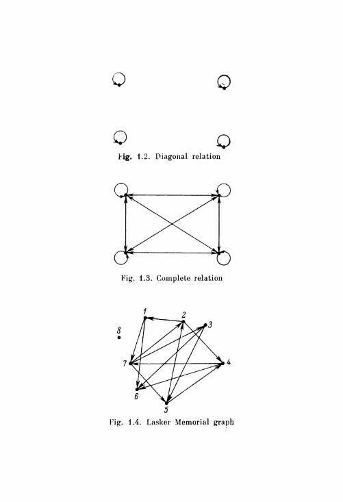
Now let M be the set of participants in a chess tournament. We shall say that “x is a vanquisher of y” if x beat y in this tournament. (It is assumed that the tournament consisted of one round.) Instead of writing down all pairs (x, y) for which the relation “to be a vanquisher of” holds, we can simply change the one-halves to zeros in the box-score of the tournament. The fact is that if participants x and y played a draw, neither of them is a vanquisher of the other. In this case, neither the relation “x is a vanquisher of y” nor the relation “y is a vanquisher of x holds. We have made the indicated changes in the box-score for the 1968 Lasker Memorial, and the result is given below. Note that it is possible to obtain complete information about the outcome of every game from our distorted box-score. Besides, if the relation “x is a vanquisher of y” holds, this does not at all mean that “x played better in the tournament than y”. The latter is an entirely different relation. Thus, “Bartsai is a vanquisher of Uhlman”, although Uhlman is higher up than Bartsai in the box-score.

In reality, we have obtained a general method of presenting a binary relation in a finite set, called the matrix method, which can be described as follows. Let M be an ^-element set in which A is a relation. Number the elements of M with integers from 1 to n. Now construct an n X n square array, whose i-th row corresponds to the i-th element of M and

Fig. 1.1. The relation “to be a standard for”. The horse, the eagle and the goat are standards in their groups

1. How a Relation is Given 21

Participants 1 2 3 4 5 6 7 8 9 10 11:12 13 14 15 16 p PI

1 B r o n ste in 0 0 0 0 1 1 0 0 0 1 1 0 1 1 110 T

I-I I

2 U h lm a n . . 1 0 1 0 0 0 0 0 1 0 1 1 1 1 110 T

I-I I

3 S u e t in . . . 0 0 0 1 1 0 0 1 0 1 0 0 0 1 1 4 III

4 V a sy u k o v 0 0 0 0 1 1 0 0 0 1 1 0 0 1 1 9 IV -V5 B a rtsa i . . 0 1 0 1 0 0 0 0 0 0 0 1 1 0 1 9 IV -V

6 Z a itse v . . 0 0 0 0 0 0 0 1 0 1 1 0 1 0 1 4 V I-V II

7 F u c h s . . . 0 1 1 0 1 0 0 1 0 0 0 1 0 0 0 4 V I-V II

8 M a lic h . . 0 0 0 0 0 0 0 0 1 0 0 0 0 0 1 8 V I I I - I X9 C zom . . . 0 0 0 1 0 0 0 0 1 1 0 0 1 0 0 8 V I I I - I X

10 M in ic h . . 0 0 1 0 0 0 0 0 0 0 0 0 0 1 1 4 X

11 H e n in g s . . 0 0 0 0 0 0 0 0 0 0 1 0 0 0 1 6 X I -X II12 Z in n . . . 0 0 0 0 0 0 0 0 0 1 0 0 0 1 0 6 X I -X II

13 R a d o v ic h 0 0 0 0 0 0 0 0 0 0 0 0 0 0 0 4 X III

14 S ch en eb erg 0 0 0 0 0 0 0 0 0 1 0 0 0 0 0 5 X IV -X V15 E sp ig . . . 0 0 0 0 0 0 0 0 1 0 0 0 0 0 0 5 X IV -X V

16 O rtega . . 0 0 0 0 0 0 1 0 0 0 0 1 0 1 0 4 X V I

whose /-th column corresponds to the /-th element of M. Place a one in the intersection of the i-th row and /-th column if the relation xtAxj holds, and a zero otherwise. Denote the element in the i~th row and /-th column by atj. The general rule for obtaining the matrix of a relation can be formulated as follows:

{1, if XiAxj holds,0, if XiAxj does not hold.

It is customary to denote the matrix consisting of elements au by || atj ||. It is obvious that this matrix contains com-

22 Ch. I. Relations

plete information about what pairs of elements from M are related by A.

Thus, a relation A in the finite set M can be given by a matrix || atj ||. The only arbitrariness lies in the choice of a numeration for M . It is easy to surmise that one can choose n\ different numerations and, correspondingly, n\ matrices describing a given relation. If an n X n matrix consisting of zeros and ones is given, and a numeration is chosen for the set M , then by the same token, a certain relation A in M is presented.

A matrix for which atj = 0 (i.e. atj = 0 for all i and /) presents the empty relation 0 , which does not hold for a single pair.

A matrix for which a^ = 1 presents the universal relation M X M, holding for all pairs.

A special role is also played by the matrix || 8*;- ||, where

x _ / 1 if i = ; ’11 1 0 if £=£/.

(The symbol 8 is called the Kronecker delta, in honour of the mathematician who first used it.) This matrix corresponds to the so-called diagonal relation E y or the equality relation: xEy if x and y are one and the same element of M .

The matrix || 8^ || has the form1 0 0 0 . . . . . . . 00 1 0 0 . . . . . . . 00 0 1 0 . . . . . . . 00 0 0 1 . . . . . . . . 0

* o

o . . o

0 . . . . . . . 1It also pays to introduce the anti-diagonal relation by

means of the condition:&ij ~ 1

A curious property is valid for the empty, universal, diagonal and anti-diagonal relations—their matrices are independent of our choice of a numeration for the elements of the set M. The reader can convince himself that this is a characteristic property of these four relations. In other

1. How a Relation is Given 23*

words, if A is a relation such that every choice of a numeration for M yields the same matrix || ||, then A is eitherempty, universal, diagonal or anti-diagonal.

There exists yet another important method for presenting binary relations in finite sets. Represent the elements of the finite set M by points in the plane. If the relation xtAxj holds, draw an arrow from xt to Xj. If xtAxiy draw a loop leaving and entering the point xt. Such a configuration is called an oriented graph, or simply a graph, and its points are called the vertices of the graph. A graph with neither arrows nor loops corresponds to the empty relation 0 .T h e diagonal relation is represented by a graph with loops only (Fig. 1.2).

The universal relation is represented by the so-called complete graph, where all pairs of vertices are connected (see Fig. 1.3).

The chess tournament box-score reproduced above can be depicted in the form of a graph without loops. For the sake of greater lucidity, this is done in Fig. 1.4 for only the first eight participants, each of whose numbers marks the corresponding vertex. The eighth vertex of this graph is isolated, since Malich drew with each of the first seven participants.

The graphs we have just introduced are geometric representations of relations, analogous to the way the graphs introduced in school were geometric representations of functions. The geometric language is helpful when the graph is sufficiently simple. On the contrary, it is more convenient to study and describe complicated graphs with large numbers of vertices in terms of relations.

One often has to consider the more general case of relations between elements of different sets M and L*. Such a relation is defined as a subset A of the set M X L. Here M X L denotes the set of pairs of the form (x, y ) where x £ M and y £ L\ Such a relation is formally defined as a triple of the form (A , M, L), where A M X L.

Ternary and, in general, n-ary relations are also considered in mathematics. An n-ary relation is defined as a subset A of M x X M 2 X . . . X M nj i.e. the set of ^-tuples of the form (xu x2, . . ., xn) where 6 In particular, all may coincide.

o 0

Q olag. 1.2. Diagonal relation

Pig. 1.4. Lasker Memorial graph

2. Functions as Relations 25

§ 2. Functions as Relations

It is possible to regard functions as a special case of relations. Let the relation A in the set M be such that for every x £ M, there exists exactly one element y 6 M for which the relation xAy holds. Thus a certain element y 6 M, determined by this condition, is associated to each element x £M. Such a relation is called a function or a mapping (or a unique correspondence), and the element y 6 M corresponding to the element x 6 M is called the value of the function A in the element x. This dependence between x and y is expressed by the notation

y = A (x).

The set A of those pairs (x, y) for which the relation holds, is called the graph of the function.

For example, if M is the real axis and A is the equality relation y = x, then the graph consists of all points of the form (x, x), and bisects the coordinate angle, i.e., coincides with the ordinary graph of the function y = x. If the relation A holds for those pairs for which z/=sin x (it is clear that for each x there exists a unique number y with this property), then the graph of A is the ordinary sinusoid.

Thus, our definition of a graph is a generalization of the ordinary definition for numerical functions.

Here it is very interesting to consider relations consisting of pairs Or, y ) where x belongs to a set M and y belongs to another set L. We shall also call a relation a of this type a function, or a mapping, if for each x 6 M there exists a unique y £ L for which xay holds. We shall write such a function symbolically as a : M -> L\ here M is called the domain of departure of the function a, and L its domain of arrival. The mapping a: M L is also called a mapping of the set M into the set L* . The element of L which corresponds to

* Unfortunately, the author likes to call different objects: pairs 04, M ) and triples 04, M, L ) —by the same name, i.e., relations. However, some authors do use distinct terms for such objects: pairs (A , M ), such that A M X M, are called relations, while triples 04, M, L), such that A c= M X L, are called correspondences. See, however, § 2, especially p. 29. {Ed. note.)


the element x of M is denoted by a (x), and is called the image of x. The element x is called the pre-image of the element a (x). It is clear from the definition of a mapping a: M — L that each element x £ M has exactly one image. However, not every element y £ L is obliged to have a pre-image. If such a pre-image exists, it may fail to be unique.

Example 1. Let M be the set of people, and L the set of natural numbers. Let a: M — L be the mapping which assigns to each person, his height, expressed in centimetres (rounded off, as is customary, to the nearest integer). It is clear that a definite height corresponds to each person, but a height of 400 cm does not correspond to any person. On the other hand, there are a great many people whose height is 172 cm.

Example 2. Let M be the set of currently living people, L the set of all people, and a: M L the mapping which assigns to each person, his father. It is clear that each x £ M has a unique image. However, not every y £ L has a pre-image, since by no means every person has been someone’s father. For example, if y is a woman. In addition, several people may have the same father.

The mapping a: M L is called surjective if each element y from L has a pre-image. In this case, it is also said that M is mapped onto L .

For example, let M be the set of all English words, L the set of parts of speech of the English language, and a : M Lthe mapping which assigns to each word, the part of speech to which it belongs. It is clear that every part of speech corresponds to at least one word—to an example for that part of speech. (We are assuming here that grammatical homonyms have already been distinguished in some way, i.e. it is known whether the word “roast” is a verb, a noun or an adjective.)

The mapping a: M — L is called injective if each element y 6 L has at most one pre-image.

For example, let M be the set of people forming a certain queue, L the set of natural numbers, and a: M ->■ L the mapping which assigns to everyone in the queue, his ordinal number. It is clear that each number can be awarded to only one person. On the other hand? this mapping is not

2. Functions as Relations 27

surjective, since there are numbers which are not awarded to anyone.

If the mapping a: M L is simultaneously surjective and injective, it is called bijective. Sets M and L, for which there exists a bijective mapping a: M -»■ L, are called equipollent. It is easy to convince ourselves that if M is finite and M and L are equipollent, then M contains the same number of elements as L. For this it is sufficient to enumerate all the elements of M, if the number n (x) is assigned to the element x G M, then the same number should be assigned to its image a (x). Since our mapping is surjective, all elements of L receive numbers. Since our mapping is injective, every element of L receives a unique number. It thus requires exactly as many numbers for the enumeration of the elements of L as for the enumeration of the elements of M. It is easy to figure out that the number of elements in these sets does not depend on how we enumerate them.

It is natural to take equipollence of infinite sets to be a generalization of the concept “having the same number of elements”.

The introduction of the following concepts is also helpful.Let a: M -> L, and let M t be a subset of M. We shall

call the set of all images {a (#)}, where x £ M lt the image of the set M l (denoted by a (A/i)). In particular, a (M ) is the image of the entire set M. It is easy to see that a: M —>■

a (.M) is a surjective mapping.Analogously, if Lx ^ L, then the union of the pre-images

of all elements in Lx is called the complete pre-image of the set Lx (denoted by a"1 (Li)),

Let us now define the so-called identity mapping of the set M:

eM:

which assigns each element x £ M to itself. (It is easy to see that the identity mapping e is the same as the diagonal relation E .) Let a : M L ; the mapping P : L ^ M is called the inverse" of a, if aP = em and Pa = eL, i.e. if P maps each image a (x) onto x , and a maps each image PXz/) onto y. In this case, we shall write: p = #a “1. The reader can easily convince himself that for the existence of an


inverse of the mapping a it is necessary and sufficient that a be bijective.

It is sometimes convenient to consider functions a : M -*■ L, which are defined not everywhere on M, but only on one of its subsets M ly which is then called the domain of definition of the functions. It then becomes convenient to add an element =[}=, not occurring in the set L, to L, obtaining thereby the new set L# = L {J {=ft=}. The element =4= plays the role of a so-called empty element. In such cases, we assume a: M — L# (but again, by definition) assigns the empty element 44 to each element of M \ M 1. It is often convenient to reason as though the empty element were already contained in an arbitrary set beforehand. It is then unnecessary to distinguish between L and L#.

Example 1. Let M be a certain set of people at a given moment, and L the set of their head-gear. Let the function a: M -> L assign to each person the head-gear he is wearing. It is clear that a is defined only on the subset of M, consisting of those people who have something on their heads. The rest, those who are bareheaded, are assigned the empty head-gear.

Example 2. Let M be the set of Russian word-forms, and L the set of Russian endings*. Let the function a assign to each word-form, its ending:

bezhat’ — at’ okno — o stolom — om

The zero (empty) endings correspond to the word-forms ustol”, “pal’to”, “vmeste”**. (The letter “o” in the word “pal’to” is sometimes taken to be a nominative case ending for the neuter gender by illiterate persons, who then attempt to decline this word. However, this isn’t a Russian ending at all, but part of the French base “paletot”.)

Even when (A, M , L) is an arbitrary relation, it may be convenient to speak of the elements y, for which xAy ,

* Because of the extreme rarity of English endings, an English example of this type wouldn’t be instructive. (Trans, note.)

** The term “zero ending” (zero morpheme) is accepted in scientific grammar. In the old orthography, a declinable noun’s empty ending \vas conveniently denoted by the hard sign: stol”, snop”, etc.

3. Operations on Relations 2$

as elements assigned, or corresponding to the element x. In such cases, the relation (A, M, L), which acquires, so to speak, a functional nature, will be called a correspondence. Thus, a correspondence is a “multiple-valued” function. When we denote an arbitrary relation ~ (A, M, L) by

M L,this will simply mean that the relation is being regarded as a correspondence.

It is clear that we could consider, instead of the correspondence \|r. M L, the function

a : M 2L,which to each element x 6 M, assigns the set Lx g= L of all those y for which (x, y ) 6 A (Lx may, in particular, be empty); however, the language of correspondences ( ^ “multiple-valued functions”) is often more convenient.

As in the case of “single-valued” functions, we can introduce the concepts of an everywhere defined correspondence (the set Lx is non-empty for every x 6 M ), an injective correspondence (Lx P| Ly = 0 whenever x == y) and a surjective correspondence (given any y £ L, there exists an x £ M for which y 6 Lx).

§ 3. Operations on RelationsBeginning with operations on sets, we can define a series

of useful operations on relations. We shall assume that all relations considered in this section are given in one and the same set M.

Thus, let us take two relations A and B . To each of them there corresponds a certain set of pairs (the subsets A ^ M X X M and B ^ M X M).

The relation determined by the intersection of the sets A and B will be called the intersection A f| B of the relations A and B. It is clear that the relation xA f| By holds if and only if xAy and xBy hold simultaneously.

Example. Let M be the set of real numbers, A the relation “to be not less than” and B the relation “to be unequal to”. Then A f| B is the relation “to be strictly greater than”. In fact, xAy is equivalent to x ^ y; xBy is equivalent to x == y.

30 Ch. I. Relations

But these inequalities hold simultaneously if and only if x > y .

Analogously, the union A U B of relations will mean the relation determined by the union of the corresponding sets. The relation xA (J By holds if and only if at least one of the relations xAyy xBy holds.

For example, if A is the relation “exceeds”, defined in a set of numbers, and B is the relation “equals”, then A [} B is the relation

It is possible to define the concept of inclusion for relations. We shall write A B if the set of pairs for which the first relation holds is contained in the set of pairs for which the second relation holds. Similarly, we shall write A a B if the set of pairs A is a subset of B y but A B.

For example, the following inclusion holds:

< c = < .

In fact, if x < yy then we automatically have x ^ y. However, there exist pairs for which x ^ yy but the relation x <C y is false. This will be the case whenever x = y.

It is very important to note the following (completely trivial) property of inclusion: if A ^ B y then xAy implies xBy. Conversely, if xAy implies xByy then A ^ B.

From this it is evident that for any relation A , we have

- 0 < = A < = U

where 0 is the empty, and U the universal, relation.We shall now introduce certain operations which are not

directly reducible to set-theoretic ones.The simplest of these is the passage to the inverse rela

tion. If A is a relation in a set M, then the inverse relation A~l is defined by the condition: xA~xy is equivalent to yAx.

For example, if A is the relation > , then A -1 is the relation <C In fact, the notation x < y is equivalent to the notation y > # . Another example: if A denotes “to be the husband of”, then A~x means “to be the wife of”.

A very important role is played by the operation denoted by A B —the product of two relations. This operation is defined as follows: the relation xABy is equivalent to the existence of a z 6 M y for which the relations xAz and zBy hold.

$ . Operations on Relations 31

Let A be the relation “to be the wife of”, and B , “to be the father of”. What does the relation xABy mean in this case? According to our definition, there exists a z, such that “x is the wife of z” and “z is the father of y”. In other words, “x is the wife of y's father”, i.e. “x is the mother or step-mother of y \

Let A be the relation “to be a brother of”, and B , the relation “to be a parent of”. Then the product AB is the relation “to be the brother of one of the parents of”, i.e. “to be an uncle of”.

A distinction was previously made in Russian (as is still done in Polish) between an uncle—a brother of the father (stryi) and an uncle—a brother of the mother (wui). This distinction is very easily formulated in terms of products of relations. Let A be the relation “to be a brother of”, B —“to be the father of” and C—“to be the mother of”. Then the relation AB is “to be a stryi of”, and the relation AC means “to be a wui of”.

We now take the well-known relations “less than” (denote it by A) and “greater than” (denote it by B) in the set of integers. The relation xABy holds if there exists a z, such that i < z and z > y. It is clear that such a z always exists— we can take, say, z = x + y + 1. Thus, in this case, AB is the universal relation.

In the next section, we shall convince ourselves that the product of relations possesses a series of nice algebraic properties, giving it a resemblance to ordinary numerical multiplication. Meanwhile, try to determine what the relation AA will be. What is this relation when A (the relation “less than”) is given on the set of all real numbers? And what relations are denoted by AB and BA when A and B are the same inequality relations, < a n d > , in the set M consisting only of the numbers 0, 1, 2, 3, 4, 5, 6, 7, 8, 9?

Let us define yet another important operation, called the transitive closure of a relation A, which will be denoted by A. The meaning of this name will be clarified by Theorem 1.5 (§ 5).

If A is some relation in a set M, its transitive closure is defined in the following way. The relation xAy is considered to hold if there exists a sequence of elements of M : z0 =


= x, zlf . . zn — y, such that the relation A holds for all neighbours, i.e.,

ZqAz j z^Azz, • • •* zn-1 Azn.In particular, this sequence may consist of only two ele

ments (n = 1): z0 = x and zx = z/. Hence, if xAz/ holds, i.e. ZqAz^ then the relation xAy also holds. This fact can be written in the form of a relation:

A ^ A . (1.1)If the sequence consists of three elements (n = 2), we have xAz and zAy. In other words, xAAy. If the sequence consists of four elements, then xAAAy. Continuing this reasoning, we conclude that xAy if and only if at least one relation of the form xAA . . . Ay (or xAny , for short) holds. Using the union operation, this fact may be written in the form of an equality:

A = A\J A2 [j A3 [} . . . []An[J ••• • (1.2)Thus, we have proven that the transitive closure of a rela

tion is the union of all powers of that relation.Let us now find out how the operations we have introduced

can be expressed in terms of operations on matrices and graphs. Since the matrices we need consist entirely of zeros and ones, it will be helpful to introduce a special (the so- called Boolean) arithmetic in the set composed of zero and one. This arithmetic is given by the following addition and multiplication tables:

0 + 0 = 0 0-0 = 0 0 + 1 = 1 0 -1 = 0 1 + 0 = 1 1-0 = 0 1 + 1 = 1 (!) 1-1 = 1.

As we see, this arithmetic differs from the usual only in that the sum of two ones is equal to one. On the other hand, performing our new operations on the numbers 0 and 1 does not lead us beyond the set consisting of these numbers. It is easy to convince oneself that the customary transformations can be carried out in this arithmetic, but only without

S. Operations on Relations 33

iimking use of subtraction: 1 —1 could be equal to zero and lo one.

We can now define operations on matrices and graphs, corresponding to our operations on relations.

Further, let us stipulate that a numeration for the set M has already been chosen, and that the matrices corresponding (under the given numeration) to the relations A and B are denoted by || aih || and || bih ||.

It is obvious thatcih — ttikbik (1«3)

is equal to one if and only if both of the relations, x%Ax and XiBxkl hold, i.e. the relation xtA f) Bxh holds. Hence, the matrix \\cih || defined by (1.3) presents the relation C = A H B. This fact can be given a somewhat different expression. Let us call the matrix || Cik ||, obtained by means of term-wise multiplication of || aik || and || bik || (according to (1.3)), the intersection || || f| || bik || of these matrices.The intersection of relations is then presented by the intersection of their matrices.

For example, let A and B be presented by the 4 x 4 matrices (M contains four elements):

0 1 0 1 0 0 1 11 0 1 1 1 1 1 10 0 1 1 - H. M = 1 1 0 01 0 1 |1 1 1 0 1

dh =

B is presented by the matrix

0 0 0 11 0 1 10 0 0 0 •1 0 0 1

In terms of graphs, intersections are defined as follows. Draw a set M of vertices, represent the relation A by dotted arrows, and the relation B by dashed arrows. Now join those and only those vertices, which are connected by both types

34 Ch. I. Relations

of arrows, by solid arrows. It is obvious that this graph represents the intersection A fl B of the relations A and B (Fig. 1.5).

1 2..................... y l

/ i4 3

AFig. 1.5. Intersection of relations

The union A U B of the relations presented by the matrices || atk || and || btk || can be similarly expressed with the aid of the operation of matrix union (addition). Namely, denote the matrix whose elements are defined by the condition

Cih = &ik "i" bih (1.4)by II cik || = || aih || + || bih ||. In formula (1.4), addition is understood in the sense of Boolean arithmetic. Having looked at the addition table for this arithmetic, we are easily convinced that Cik = 1 if and only if at least one of the summands, ath or bihl equals one. Hence, cih = 1 is equivalent to xiA U Bxk.

The union of the two relations presented above by 4 X 4 matrices is presented by the matrix

0 1 1 1 1 1 1 1 1 1 1 1 *1 1 1 1

The graph of a union is constructed by drawing an arrow between all vertices which are joined by at least one kind of arrow. Taking graphs A and B from Fig. 1.5, we obtain the graph of their union, as depicted in Fig. 1.6.

II C*k || —

S. Operations on Relations 35

The product AB of relations is presented by the so-called matrix product. This operation on matrices, which plays an important role in algebra, is defined by the following rule:

Cik = CLiibik + O ' i ^ k - f • • • + Uinbnky

or, using the customary abbreviated notation for a sum,n

C i h — 2 ^ i j b j k • (1*5)i = i

Here the number n denotes the order of the matrices—the number of elements in the set M. In spite of the simplicity of the asserted connection between the products of relations and matrices, let us carry out the necessary proof.

/ 2

AUB

Fig. 1.6. Union of relations

Let the relation xiABxh hold. We shall show that the number calculated in accordance with (1.5), is equal to one. In fact, by the definition of the product of two relations, there exists an element xj 6 Af, such that xtAxj and X j B x k . This means that atj = bjk = 1. Hence aijbjk = 1. But according to the rules of Boolean arithmetic, if one of the summands is equal to one, then their sum (1.5) is automatically equal to one, i.e. cik = 1. Conversely, let cik = 1. Then at least one of the summands in (1.5) is equal to one. Let atjbjk be such a summand. But the product equals one only if atj = bjh = 1. Now this means that xtAxj and XjBxk, i.e. XiABxk.

Thus, we have proven that the product of two relations corresponds to the product of their matrices.

36 Chm / . Relations

The graphical interpretation of the product is as follows. Let the relation A again be represented by means of dotted, and B , by dashed, arrows. Join the vertices xt and xk with a solid arrow if it is possible to pass from xi to xh in the following way: first go from xf along a dotted arrow to some xj, and then from xj along a dashed arrow to xk (Fig. 1.7). These new arrows represent the product AB.

It is obvious from Fig. 1.7 that our method for constructing the graph of the product of relations resembles the

Fig. 1.7. Product of relations

parallelogram method for adding velocities or forces. This resemblance is not accidental. Let M be a set of points in the plane, and let the relation xAy (respectively: xBy) mean that moving with speed a (respectively: 6), one can get from point x to point y in a unit of time. Then xABy means that moving with speed a + b, one can get from x to y in a unit of time.

The operation A~l is expressed quite[simply in matrix form. If A is presented by the matrix || aih || then A~l is presented by the matrix || atk ||, in which rows and columns have changed places: a ik = aft*. In other words, the matrix for A~l can be obtained from the original matrix by means of a reflection in the main diagonal. In fact, if aik = 1, then XiAxk and xhA~xXi, i.e. a ki = 1. But if aik = 0, then a k(=0.

Example.0 1 1 1 0 1 0 01 1 0 0 1 1 1 10 1 1 0

t1

1 0 1 00 1 0 0 1 0 0 0

4. Algebraic Properties of Operations 37

In order to obtain the graph representing A~x from the graph representing the relation A, we must change the direction of each arrow and leave all loops as are.

The operation A of transitive closure can be expressed in matrix form by the union of the powers of A fs matrix, according to Formula (1.2). It is more intuitive to pass from the graph representing the relation A to the graph representing^.

Fig. 1.8. Transitive closure of a relation

Indeed, it follows from the definition of the transitive closure that the vertices Xi and xk are joined by an arrow in the new graph if there is a path in the original graph leading from xt to xh in the same direction as the arrows. The graph of the relation A is depicted in Fig. 1.8. It is obvious that from each of its vertices, there exists a path leading to an arbitrary, perhaps the same, vertex. Thus, in the case under consideration, the relation A corresponds to the complete graph.

§ 4. Algebraic Properties of Operations

Since1 the operations of intersection and union of relations arose from the set-theoretic operations of intersection and union, all properties of the former operations are exactly the same as those of the latter.

Let us now examine algebraic properties of the remaining operations.

38 Ch, / . Relations

The inversion operation has an important property. It is expressed by the equality

( A ^ y ^ A . (1.6)In fact, x {A~l)~ly is equivalent to yA~lx, But the latter is equivalent to xAy.

The multiplication operation, unlike multiplication of ordinary numbers, is not commutative: in general, AB =£ =£ BA . This can be seen by working out a simple example, when the relations have the following matrix presentations:

A

1 1 0 0 1 1 0 0 0 0 1 1 0 0 1 1

B

1 0 0 0 0 1 1 0 0 1 1 0 0 0 0 1

In this case, we have

AB

1 1 1 01 1 1 00 1 1 10 1 1 1

BA

1 1 0 01 1 1 11 1 1 10 0 1 1

We leave the computations to the reader, who can easily obtain them from the graphical representations (see Fig. 1.9,

Fig. 1.9. Example of non-comrautativity of the product

where A is depicted by dots, and B, by dashes. It is assumed that there are also two loops at each vertex—one dotted and the other dashed.


When the product of two relations does not depend on their order: AB = BA , we say that A and B commute.

It is easy to verify that the diagonal relation E plays the role of an identity:

AE = EA = A (1.7)for any relation A.

Analogously, for the empty relation we haveA 0 = 0 A = 0 . (1.8)

In fact, x 0 A y cannot hold for even a single pair, since x 0 z never holds. The equality (1.8) means that with respect to the multiplication of relations, the empty relation 0 behaves in the same way as zero does in ordinary numerical multiplication.

The associative law turns out to be valid for the multiplication of relations:

(AB) C = A (BC) (1.9)

For if x (AB) Cy, then there exists az, such that xABz and zCy. xABz implies the existence of a w, such that xAw and wBz. It follows from wBz and zCy that wBCy. We obtain xA (BC) y from xAw and ’ wBCy. Similarly, it is easy to derive x (AB) Cy from xA (BC) y. Thus (1.9) is proven.

The associative law enalVes us to do without parentheses in products/and to simply write: ABC, ABCD, etc. Instead of products of the form AAA, A AAA, we shall write the powers A 3, A4, . . .*.

Let us now consider properties connecting the various operations.

The simplest of these is the rule for inverting products: (AB)"1 = (1.10)

In fact, x (AB)~ly means' that yABx, i.e. there exists a z, for which yAz and zBx. But this means that xB~xz and zA~ly, i.e. xB~xA~xy.

* Associativity of the multiplication of relations and the notation An was already used in § 3 (see (1.2)).

40 Ch. I. Relations

Another property connecting the inversion and product operations consists of the following: if for each x there exists a z, such that xAz, then

A A - ' ^ E . (1.11)

In fact, xAz implies zA~lx, i.e. xAA~xx. But xEy means that x = y. Hence, it follows from xEy that xAA~ly.

Analogously, if for each x there exists a z, such that zAx, then

A - ' A ^ E . (1.12)

The properties we have proven mean that for relations which do not hold too rarely (each element x is related by A to at least something or other), the inversion operation resembles the numerical operation of passing from a to a"1: the inclusions (1.11) and (1.12) are close to the numerical equality a~xa — 1, since E , as we have already stated, plays the role of an identity.

The next two properties connect the product operation with the intersection and union. They resemble the distributive law of multiplication over addition. The first of these “distributive laws” has the form

(A U B)C = (AC) U (BC) (1.13)

It can be proven in the following way. We first assume that the relation x {A U B) Cy holds. This implies the existence of a z, such that at least one of the relations xAz, xBz holds and the relation zCy holds. Then xACy or xBCy holds. Hence the relation x (AC) [j (BC)y holds. Conversely, let x (AC) U (BC)y hold. This means that xACy or xBCy, i.e. there exists a zx, for which xAz1 and zxCy, or there exists a z2, for which xBz2 and z2Cy. But since A ^ A [] B and B s A IJ B, in the first case we have x (A [j B) zx and zxCy, i.e. x (A [] B) Cy. In the second case: x (A [] B) z2 and z2Cy, i.e. once again x (A [j B) Cy. Thus, the validity of the left side of (1.13) follows from that of the right side, and conversely. By the same token, the equality (1.13) is proven.


The second “distributive law” has the weaker form of an inclusion:

(a n b ) c ^ ( a c ) n (b c ). (i.i4>Suppose that the relation x (A f] B) Cy holds. This means that there exists a z , such that the relations xAz, xBz and zCy hold simultaneously. Hence, the following pairs of relations hold simultaneously: xAz, zCy and xBz, zCy. In other words, xACy and xBCy, i.e. x (AC) f| (BC) y. Q.E.D.

However, the inclusion in (1.14) cannot be changed to equality. We show this by defining A, B, C in the four- element set M = {x!, x2, x3, xA} by requiring that the following relations, and no others, hold (Fig. 1.10): xxAx2, xxBx3, x2Cx^ x3Cxa. It is clear that A f| B = 0 . So according to (1.8), we have ( 4 f| B)C = 0 . On the other hand, xxACx^ and xxBCx4. Consequently, x1 (AC) f| (BC) #4, i.e. (AC) f) (BC) == 0 . In this case, we have the strict inclusion

(A n B)C a (AC) fl (BC),which demonstrates the impossibility of replacing inclusion by equality in (1.14).

Verification of the following simple properties of relations will be left for the reader:

(A\)B)-' = A~1\JB~\ (1.15)(A(\B)-' = A-'(\B~K (1.16)

The following important property is valid for the transitive closure operation:

if A ^ B , then i g f i , (1.17)

42 Ch. I. Relations

We leave the proof for the reader. Analogously, a similar “monotonicity” is valid for other operations, namely:

(1) if A ^ B , then A'1 s fl"1; (1.18)(2) if A ^ B , then A C ^ B C and CA<=CB. (1.19)

Finally, the following property is obvious:

i = i (1.20)We have apparently exhausted the main properties of

operations, which are valid for arbitrary relations. We shall study algebraic ^properties of these operations for certain special classes of relations in future chapters.

As preparation for this, we define certain new operations in terms of the original ones:

(1) the symmetrized product—A o B = AB U BA;

(2) the transitive closure of the union—^ / X

A \jB = A[}B;(3) the transitive closure of the symmetrized product—

^ / XA o B == A o B .

It is clear from the definition that these three operations are commutative.

However, the associative law does not always hold for the symmetrized product. In fact, using the distributive law proven above, we compute two triple products:

(AoB)oC = (AB U BA) C U C(AB U BA= ABC[jBAC[}CAB[}CBA, and (1.21)

Ao(BoC) = A{BC[) CB) U (BC U CB) A = ABC U ACB U BCA U CBA.

If A and C commute, then

BAC U CAB = BCA U ACB.

(1.22)

5. Properties of Relations 43

Comparing this equality with (1.21) and (1.22), we obtain that when AC = CA,

{A o B) o C = A o {B o C).

In particular, the associative law is true when all three relations 7commute. Then (A o B) © C = A © (B © C) = ABC.

It will be an instructive exercise for the reader to actually construct three relations for which the associative law fails to hold.

§ 5. Properties of RelationsIn this section, we shall deal with some important pro

perties of relations which, later on, will permit us to single out significant classes of relations.

Definition 1.1. The relation A is called reflexive if E s A. In other words, a reflexive relation always holds between an object and itself: xAx.

Informal examples of reflexive relations: “to resemble”, “to have some feature in common with” (if every object has at least one feature), “to be not older than”. On the other hand, such relations as “to be a brother of”, “to be older than” are clearly not reflexive.

A reflexive relation can always be represented by a matrix, all of whose principal diagonal entries are equal to 1. In a graph representing a reflexive relation, every vertex has a loop. Because of this fact, we shall omit suclTloops from diagrams of relations known to be reflexive.

Definition 1.2. The relation A is called antireflexive if xAy implies x == y, i.e., in algebraic notation, A f| E = 0 . In other words, A ^ = =, i.e. A can only'hold for distinct objects.

The relations mentioned above as examples of non-reflexive relations are antireflexive. The relation “to be a standard for” will, in general, be neither reflexive nor antireflexive.

All principal diagonal entries of a matrix representing an antireflexive relation are equal to 0, and the corresponding graph cannot have any loops.

Difinition 1.3. The relation A is called symmetric if A ^ A~l . In other words, if xAy holds, then yAx also holds.

44 Ch. I. Relations

Informal examples of such relations are “to resemble”, “to be the same as”, “to be a relative of”.

In a matrix representing a symmetric relation, entries symmetrically situated with respect to the principal diagonal are equal to each other:

O'ih— O'hi •In the corresponding graph, along with each arrow going

from vertex Xi to vertex xk, there exists an arrow with the opposite orientation. Therefore, we can omit all arrows from such a graph, and confine ourselves to drawing loops and line segments connecting distinct vertices. In other words, a symmetric relation is naturally represented by an unoriented graph. This is how we shall henceforth represent the graph of a relation known to be symmetric.

Theorem 1.1. The relation A is symmetric if and only ifA = A-K

Proof. By definition we have A ^ A~l, which, by virtue of (1.18), yields

A~l s= (A '1) -1.

Hence, according to (1.6), we obtainA"1 ^ A.

Comparing this inclusion with the original one, we arrive at the conclusion that A = A ~1. The converse is obvious.

Definition 1.4. The relation A is called asymmetric if A n A - 1 = 0 . This means that at least one of the two conditions xAy and yAx fails to hold.

This leads to the following equality for matrix entries:aihahi = 0. (1*23)

In the corresponding graph, there can be no arrows joining two vertices in opposite directions, i.e. it is always essential to indicate the direction of an arrow.

Theorem 1.2. If the relation A is asymmetric, then it is antireflexive.

Proof. Let us suppose that xAx holds for some x. Then xA~lx would also be true, i.e. xA f| A~xx. But then the relation A f| would not be empty.

5. Properties of Relations 45

We could also have derived this fact from our equality for matrix entries: setting i — k in (1.23), we obtain a\h = 0, i.e. ahh = 0.

It follows from Theorem 1.2 that the graph of an asymmetric relation can have no loops.

Difinition 1.5. The relation A is called antisymmetric if A f) A ' 1 ^ E. This means that xAy and yAx can hold simultaneously only in case x y.

This leads to the following assertion for matrix entries:aikCtki = 0 if i=^=k.

Definition 1.6. The relation A is called transitive if A 2^ A . Developing this algebraic condition, we arrive at the following: if xAz and zAy, then xAy also holds. Hence, by induction, we obtain: if xAzly z1Az27 . . ., zn-i A y , then xAy.

This property can be readily interpreted in terms of the graph representing A. Namely, if x is connected to y by a path moving in the direction of the arrows, then there exists an arrow going directly from the vertex x to the vertex y.

Remark. It is not difficult to show that for a reflexive relation A, transitivity is equivalent to A 2 = A.

Theorem 1.3.1/ A is transitive, then A = A . In other words, a transitive relation coincides with its own transitive closure.

Proof. We shall first prove the following inclusion for a transitive relation A:

A n c=A. (1.24)Indeed, for n = 2, this is the definition of a transitive relation. Assume that (1.24) has already been proven for some n. Then An+1 = AnA by associativity; taking into account our inductive assumption (1.24) and (1.19), we have

An+1 = AnA s AA s A.Thus, we have successfully carried out the induction step. We now turn to Formula (1.2), defining the transitive closure of A t and replace every term of the union by a larger one, according to (1.24). We obtain

A = A U ^2U^3U . . . U ^ nU . - - ^ ^ U ^ U . . - U ^ U . . . - ^ .

Ch. / . Relations46

Thus, i g i . But, on the other hand, according to (1.1), we always have A ^ A . Hence A = A. The theorem is proven.

It is easy to see that the converse also holds.Theorem 1.4. If A = A, then A is transitive.Proof. It follows from (1.2) that A2<=A. Since A = A,

we have A 2^ A .

Theorem 1.5. For any relation A , the transitive closure A is equal to the intersection f] B of all transitive relations B containing A .

Proof. Since A = A, it follows from Theorem 1.4 that A is always transitive. Besides, A ^ A . Hence, A is one of the B's figuring in the theorem. Consequently, A ^ f) B. In order to prove the reverse inclusion, suppose that B is an arbitrary transitive relation containing A. Thus, A <=: B. By (1.17) A ^ B. But, by Theorem 1.3, B = B . Therefore, A <=: B. The theorem is proven.

If the relation 04, M) is a restriction of the relation 04u M x), all the above properties which hold for the latter are automatically true for the former. Thus, the reflexivity of 04lf M ±) implies that of its restriction (A, M). In fact, if xAxx is true for all x 6 M ±, then xAx will also hold for all x 6 M. The symmetry of (Al9 M x) implies that of its restriction, since for all x 6 M and y £ M, yAx follows from xAy. The truth of our assertion for the remaining properties is left for the reader to verify.

§ 6. Invariance of Properties of Relations

In this section, we shall study cases where one or another property of the result of operating on relations is determined by similar properties of the operands *.

* It is worth-while noting that the author uses the term “lemma” in a somewhat non-standard manner. He calls not only auxiliary assertions, but also theorems which are simply less significant, lemmas. (Ed. note.)

6 . Invariance of Properties of Relations 47

Lemma 1.1. If the relations A and B are reflexive, then so are the following relations:

A[}B, A{] B, A-1, AB, A.

The proof immediately follows from the appropriate definitions. For example, it follows from xAx and xBx that the relation xA f| Bx, and a fortiori xA U Bx , holds.

The situation is somewhat more complicated when dealing with antireflexivity. In this case we have

Lemma 1.2. If the relations A and B are antireflexive, then so are the following relations: A U B, A f) B,A~X.

The proof of these assertions can be carried out just as easily as for the preceding lemma.

As for the product AB and the transitive closure A of antireflexive relations, they can very well fail to be antireflexive*. The relation A , defined in a two-element set M by the matrix presentation

can serve as an example. It is easy to see that the square of this matrix presents a reflexive relation,

A2

and the transitive closure of A,

as a universal relation, is also reflexive. The reader would be well-advised to draw the corresponding graphs.

Let us now examine the behaviour of relational symmetry under various operations.

Lemma 1.3 . I f the relations A and B are symmetric, then so are the following relations: A U Z?, A f| By A -1.

*It is easy to see that the product AB of antireflexive relations A and B is antireflexive if and only if A f t B - 1 = 0 . (Ed. note.)

48 Ch. I. Relations

Proof. By virtue of (1.6) and Theorem 1.1, we have {A _1)~1 — = A = A~lt i.e. the relation A~l is also symmetric. From the equality (1.15) we obtain

( A U B F ^ A ^ U B - ' ^ A U B ,i.e. the union A (J B is symmetric. From the equality (1.16) we obtain

and the symmetry of the intersection is therefore proven.As for the symmetry of the product, a complete answer is

given byLemma 1.4. In order that the product AB of symmetric

relations A and B be symmetric, it is necessary and sufficient that A and B commute.

Proof. Let AB = BA. Then, according to (1.10), we have

(.ABy1 = {BA)-1 = A~xB“l = AB,i.e. the product AB is symmetric. Conversely, if AB is symmetric, then by Theorem 1.1 AB = (AB) -1. But then by (1.10) we obtain AB = (AB)~l = B~lA ~l = BA , i.e. AB = BA. The lemma is proven.

Readers familiar with linear algebra must have certainly guessed already that this theorem is simply a variant of the well-known theorem to the effect that the product of symmetric matrices is symmetric if and only if these matrices commute.

Corollary. The transitive closure A of a symmetric relation A is a symmetric relation.

For it is easy to derive from Lemma 1.4 and (1.9) that the relations A2, A 3, . . ., A71, . . . are symmetric. But then, by(1.2) and a natural generalization of Lemma 1.3, the transitive closure

A = A [ ) A 2{JA*{) . . .is also symmetric.

The reader would be well-advised to prove this assertion directly from the definition of the transitive closure, without making use of Lemma 1.4.

As for the property of asymmetry, we have

6. Invariance of Properties of Relations 49

Lemma 1.5. (1) If the relation A is asymmetric, then the intersection A f| B is asymmetric for any B. (2) If the relation A is asymmetric, then so is A~x.

Proof. (1) According to definition 1.4, A f| A~* = 0 Thus, by (1.16) we have{A[\B){\(A[\B)~' = A[\B[\A~'[\B~' = A[\A~'[\B[\B~' =

= 0 f ] Bf ) B - ' = 0 ,i.e. A fl B is asymmetric.

(2) Similarly, taking (1.6) into account, we obtainA-* n 04- t 1= a * n a = a n ^ = 0 ,

which means that inversion preserves asymmetry.The union of asymmetric relations can very well fail to

be asymmetric*. Neither are the product and transitive closure of asymmetric relations necessarily asymmetric.

Lemma 1.6. If the relation A is antisymmetric, then so are the following relations: A f| B, A~x.

Proof. We can practically reproduce our previous reasoning for the inverse relation. For the intersection, our proof nearly coincides with that of Lemma 1.5:(A(]B)(]{A{] B y 1 = (A fl A~') fl (B fl S"1) <=E[\(B() B-*) =E.

Antisymmetry can fail to be preserved under the union **, product and transitive closure of relations.

As for transitivity, we can assert the following:Lemma 1.7. If the relation A and B are transitive, then

so are the following relations:A(\B, A'1, A.

Proof. Let the relations xA f] By and yA f| Bz be valid. Then so are xAy, yAz, xBy and yBz. Hence, by virtue of the transitivity of A and B, we have xA fl Bz, i.e. A f| B is transitive. If xA~xy and yA~xz hold, then by the definition of the inverse relation, we have zAy and yAx, i.e. zAx and xA~xz. This means that A is transitive. Finally, the transitivity of A follows from (1.20) and Theorem 1.4.

* The union A U B of asymmetric relations A and B is asymmetric if and only if A fj B - 1 = 0 . (Ed. note.)

** The union A (J B of antisymmetric relations A and B is an tisymmetric if and only if A f| B ' 1 £ E. (Ed. note.)

Chapter

IIIDENTITY AND EQUIVALENCE

§ 1. From Identity to Equivalence

In ordinary discourse, we often speak of the identity (equality) of certain objects (things, sets, abstract categories), without concerning ourselves with the exact meaning to be properly conveyed by the word “identical”. Let us try to grasp this meaning by analysing various situations, where we confidently regard certain objects as identical.

Take a standard set of chess-pieces. All of its white pawns are identical from the point of view of a chess-player. When setting them up on a chess-board, a chess-player will take them out of a box in an arbitrary order. They will all be in the second rank when the game begins, without the chessplayer having thought of where it would be best for him to place a randomly chosen pawn. When the pieces are being set up before a game, either of the black rooks can, in just the same way, wind up equally well on the king’s or queen’s side. These rooks are identical.

But imagine a different situation: this same chess-set is given to a child who is playing soldiers. In his game, distinct pawns can acquire individuality, names and markings. However, as soon as this same child starts using the chess- pieces properly, pawns of the same colour become identical once more.

Take another situation: chess pieces in the course of a game. Suppose the chess-player is faced with the following choice: should he sacrifice a pawn which has already advanced to the seventh rank and is about to be queened, or a pawn which is peacefully standing in opening position? It is

511 . From Identity to Equivalence

clear that (everything else being equal) the first pawn is far more valuable, and the chess-player no longer regards these two pawns as identical. True, the objects in this situation aren’t the wooden pieces in themselves, but “pawns in given positions”. Since each pawn plays its own individual role at each point of the game, they are, of course, not identical for a good chess-player.

Here we see the same kind of difference as between a word in the English language and a word in a given context. For example, the words “pawn” and “pawn”, although printed in different scripts, are identical as English words. But in the contexts “The grandmaster sacrificed his pawn brilliantly” and “He was only used as a pawn”, this word has different meanings. To put it another way, the words are identical, but the meanings differ.

Analogously, we may speak of the identity of people in different senses. From the professional point of view of a retail clothes sales clerk, people of one and the same sex, height and size are indistinguishable. However, a good sales clerk distinguishes customers according to their tastes, and a good tailor understands that there are, in addition to height and size, individual peculiarities of the figure. But for a stock clerk distributing uniforms (snow suits, say, for mountain climbers), only size has any significance. It is of little significance to an anatomy professor whose corpse he uses for demonstrating the structure of human organs to his students. But there can be no identical patients for a psychiatry professor.

From the point of view of a personnel director, people with the same vitae are identical. But there are no identical, interchangeable scientists for a laboratory head.

When we invite guests, it makes a world of difference to us who comes and whom they bring with them. From the point of view of mutual relations of individual persons, no two people are equal. When speaking of the universal equality of human beings, we have in mind equal rights before the law, the equal value of individuals, but not the equality of individualities.

Consider the set of animals depicted in Fig. 2.1. We have divided them into the following six groups: (1) terrestrial mammals, (2) marine dwellers, (3) insects, (4) birds, (5)

Fig. 2.1. Equivalence classes

1. From Identity to Equivalence 53

mythologicalTbeings and (6) reptiles. We shall consider the animals occurring in a single group to be identical by definition. It is possible to imagine a situation where animals identical in this sense are interchangeable. For example, when a biology teacher has to show his pupils representatives of different types.

If we carefully analyse what is common to the uses of the word “identity” in all of the above examples (and also in the examples which the reader can now make up by himself), then we see the following. First, identity is always understood as a binary relation in a certain set of objects. Second, the content of this relation depends on the situation in which we are considering these objects, or on the observer, who passes judgement on the identity of objects from his chosen point of view. Third, the word “identity” turns out to be synonymous with the word “interchangeability” (of objects in a given situation).

In fact, the identity of white pawns, or of other pieces having the same name and colour, consists in our ability to replace any of them by another. Whatever be the script used for printing a word in a dictionary, it remains the very same word. It seems exceedingly natural to assume that objects are interchangeable in a given situation if and only if they possess one and the same collection of formal features, significant in that situation. We shall convince ourselves in the next section that this assumption is correct and can be given a precise meaning, if we formulate the concept of identity, or interchangeability, precisely.

Now let M be a set of objects, some of which are interchangeable. Denote the set of all objects interchangeable with the object x by M x. It is obvious that x £ M x, and so the union of all M x (for all possible x in M) coincides with the entire set M:

M = U Mx (2.1)x£M

Suppose that M x f| M y == 0 . This means that there exists some element z, which belongs to M x and M y simultaneously. Hence, x is interchangeable with z and z is interchangeable with y . Consequently, x is interchangeable with y, and so also with any element in M y. Thus, M x ^ M y. A symmetri-

54 Ch. II . Identity and Equivalence

cal argument shows that M y ^ M x. Thus, the sets M x occurring in the union (2.1) either coincide completely, or else are disjoint.

The reasoning carried out above suggests how one can rigorously define the concept of identity, or interchangeability. In connection with this, it is worth-while noting how words are used in mathematics. Until now, we have been dealing with the words “identity” and “interchangeability” (in a given situation). These words have in no way been defined, but have been used as we are accustomed to employ them in ordinary discourse. But now, when we want to give a precise definition (explication), we choose a new name. Namely, we now define the relation of equivalence, which is the explication of the concept of identity. The above discussion should be regarded as motivation for precisely such an explication.

Definition 2.1. We shall call a system* {Mly M 2j . . .} of non-empty subsets of a set M a partition of that set, if

(1) M = M 1 U M 2 U • . . and

(2) Mi f) Mj = 0 for i /.The sets M x, M 2, . . . are called the classes of the given partition.

Definition 2.2. A relation A in a set M is called an equivalence (or an equivalence relation), if there exists a partition {Mx, M 2, . . .} of the set M, such that the relation xAy holds if and only if x and y belong to some common class M t of that partition.

Let {A/j, Af2, . . .} be a partition of a set M . Beginning with this partition, let us define a relation A in M: xAy if and only if x and y belong to some common class M t of the given partition. It is obvious that the relation A is an equivalence. We shall call A the equivalence relation corresponding to our initial partition.

For example, a partition of a certain set of animals into six subsets is depicted in Fig. 2.1. The corresponding equivalence relation is the identity relation defined above.

* It is completely immaterial to us whether this system is finite or infinite.

1 . From Identity to Equivalence 55

Another example: the partition consists of subsets of a set M, containing exactly one element each. The corresponding equivalence relation is the equality relation E. Finally, if the partition of a set M consists of a single subset, coinciding with M itself, then the corresponding equivalence relation is the universal relation: any two elements are equivalent.

The reader can easily convince himself that the empty relation (in a non-empty set!) is not an equivalence.

We arrived at equivalence through the concept of interchangeability. But what is meant by the assertion that two objects, x and y, are interchangeable in a given situation? This can always be understood to mean that each of them contains all information about the other, which isn’t immaterial in the given situation. This assertion isn’t so very profound; it only means that the interchangeability of objects is the coincidence of the features which are significant in a given situation.

For example, let us regard cars of one and the same model, produced in one and the same factory, as identical. Then, having taken apart one “Volga”, we can draft a complete set of patterns, which can be used for producing “Volgas” of the same type. However, having studied one “Volga”, we can’t guess what colour another car of the same model is painted, or what kind of dents there are on its bumpers.

When we choose one piece from a chess-set, we know where it can be placed in starting position and how the pieces interchangeable with it, i.e. of the same name and colour, move. In the example with the animals of Fig. 2.1, if we choose the winged horse—Pegasus, then by the same token we already know that all animals equivalent to it are of mythological origin. And this is precisely all the information that is significant in the given classification.

Everything is very primitive in the case under consideration—an object contains within it complete information about each of the objects equivalent to it, and carries no information about any other object. But for other types of relations (cf. Chap. Ill), this idea of evaluating the information, contained in a given object about another object, can be somewhat more deeply developed,

56 Ch. I I Identity and Equivalence

Now let there be given a partition {Mly M 2, . . .} of a set M. In each set M t, choose some element xt contained in it. We shall call this element a standard for each element y occurring in the same set M t. We shall assume—by definition—that the relation XiAy holds. We shall call the relation A, defined in this way, a relation “to be a standard for”.

It is easy to see that the equivalence C4), corresponding to an initial partition, can be defined as follows: y (A) z if y and z have a common standard: XiAy and x%Az.

It is clear that any equivalence relation can be so defined in terms of a relation “to be a standard for”, and conversely, any relation “to be a standard for” defines some equivalence.

Let A be an equivalence relation, and let StA be a relation “to be a standard for”, such that xAy holds if and only if x and y have a common standard z.

In other words, xAy is equivalent to the existence of a z , such that zStAx and zStAz/. Since zStAx = x (StA)-1z, this means that

A — (StA) 1 StA.In other words, equivalence can be expressed algebraically

in terms of a simpler relation, “to be a standard for”. The fact that “to be a standard for” is simpler is evident from the following considerations. The relation StA in a set of n elements can be represented by a graph having exactly n-m arrows, where m is the number of equivalence classes: each element is connected to its unique standard*. The graph depicting the equivalence relation consists of m complete subgraphs, each containing nt vertices (nx + + • • •. . . + nm = n). Thus, the total number of edges in this graph is equal to

mS *i (»i—i)

2i=l

Example. Partition the set M of all non-negative integers into the set M 0 of even numbers and the set Mx of odd number. The corresponding equivalence relation is denoted as follows:

n == m (mod 2)* It isn’t necessary to connect a standard to itself.

2. Formal Properties of Equivalence 57

which is read: n is congruent to m modulo 2. Here it is natural to choose 0 as the standard for even numbers, and 1 for odd numbers. Analogously, partitioning the same set M into k subsets Af0, Afx, . . M h-ly where M j consists of all numbers leaving the remainder ; on division by k , we arrive at the equivalence relation:

n = m (mod k),

which holds if n and m leave the same remainder on division by k. As the standard for each Mj, it is natural to choose the corresponding remainder j.

§ 2. Formal Properties of Equivalence

We have defined equivalence relations above with the aid of partitions, i.e. actually given them by means of a certain construction. We could have defined equivalences differently: by formulating properties (axioms), which distinguish equivalence relations from other binary relations. Instead of Definition 2.2, we can introduce the following

Definition 2.3. The relation A in a set M is called an equivalence (or an equivalence relation), if it is reflexive, symmetric and transitive.

We have now violated mathematical etiquette, in that we have given two independent definitions for one and the same concept. We have done this in order to demonstrate and compare two different methods for introducing mathematical concepts: constructive and axiomatic. But now we should convince ourselves that nothing else except etiquette has been violated, i.e. that our two definitions are equivalent. The necessary justification will be found in

Theorem 2.1. If the relation A in a set M is reflexive, symmetric and transitive, then there exists a partition {M 1, Af2, ...} of M, such that xAy holds if and only if x and y belong to a common class of the partition.

Conversely: if the partition {M Af2, . . .} of a set M is given, and the binary relation A is defined as “belong to a common class of the partition”, then A is reflexive, symmetric and transitive.

Proof of the first part. Consider the reflexive, symmetric and transitive relation A in M. For any x 6 M } let the set M$ consist of all elements zt for which xA%.

58 Ch. I I . Identity and Equivalence

Lemma. For any x and y, either M x = M v or M x f| M v = 0 .Proof of the lemma. Suppose that the intersection M x f)

fl M v is not empty. We shall show that M x = M jr Let z £ M x fl M y; then xAz and yAz hold by the definition of the sets M x and M lf. By symmetry we have zAy, and by transitivity, xAy follows from xAz and zAy. Now take an arbitrary element w £ M y. By definition yAw. But xAy and yAw imply xAw, i.e. w £ M x. Thus, M y ^ M x.

Take an arbitrary element v £ M x; xAv holds for it. By the symmetry of the relation A , we have yAx. But yAv follows from yAx and xAv. Hence, v £ M v. By the same token, we have shown that M x M u. Summing up, we can conclude that M x = Mv. The lemma is proven.

It follows from the lemma and the reflexivity of A that the sets of the form M x constitute a partition of M. (It is natural to call this partition the partition corresponding to the original relation.) Now let the relation xAy hold. This means that y £ M x. But x £ M x in view of xAx. Consequently, both of the elements x and y occur in M x. Thus, if xAy, then x and y occur in a common class of the partition. Conversely, let u £ M x and v £ M x. We shall show that uAv holds. In fact, we have xAu and xAv. Hence, by symmetry, we have uAx. By transitivity, uAv follows from uAx and xAv. The first part of the theorem is proven.

Proof of the second part. Suppose the partition {M\, Af2, • • .} of a set M is given. Since the union of all the classes of the partition coincides with M, each x £ M occurs in some class M t. From this it follows that xAx, i.e. the relation A is reflexive. If x and y occur in the class M h then y and x occur in the same class. This means that xAy implies yAx, i.e. the relation A is symmetric. Now suppose that xAy and yAz hold. This means that x and y occur in the class M t, and y and z in the class M j. Since M t and M 7- have a common element y, they coincide. Hence, x and z occur in M t, i.e. xAz holds. Thus, the relation A is transitive, which completes the proof of Theorem 2.1.

Note that nowhere have we used any assumption about the finiteness of the set M or of its partition.

From the theorem we have just proved, we easily obtainTheorem 2.2. If M is a finite set and A is an equivalence

relation in it, then there exist an n and an m, such that one

2. Formal Properties of Equivalence 59

can assign to each element x £ M a string (ordered collection) of n + m dyadic features (zeros or ones):

% (5l» • • • * ?n+i» • • • i

y ■“*" ('Hi? ^2* • • • > |ni ‘Hn+l* • • •» 1n+m) etc.,

in such a way that (1) distinct strings of features correspond to distinct elements and (2) in order that xAy, it is necessary and sufficient that the first n features of these elements coincide:1 ’Hit 2 ^2’ •••> \n ln*

Proof. Take the partition {Mx, M 2, . . .} of the set M, corresponding to the relation A. In view of the finiteness of M y this partition is finite and each of its classes is finite. Number the elements of each class. Then we can assign a pair of integers to each element x: x — (p, q), where p is the number of the class Mp in which x lies, and q is the number of x within its class. It is clear that if x ->• (p1? qx ), y — -> <p2* ?2> and Xz£ y, then (p1? qx) ^ (p2 » 2>* In fact, either x and y lie in different classes—then their first numbers are distinct: px p 2; or else their numbers within theirclass are different—then q± q2. Now write down the dyadic expansions for the numbers p and q. Let n be the greatest number of digits obtained for the p’s, and m, the greatest number of digits obtained for the q's. If there are less than n digits for some p, then add zeros on the left. Treat the second numbers similarly. Thus, a string of n + m dyadic features will be assigned to each element.

In order to complete the proof, it is sufficient to note that, the equivalence of two elements means their occurrence in a common class, i.e. the coincidence of their first n numbers (features).

This theorem justifies our previous assertion that any equivalence (true, in a finite set) can be given as the coincidence of a certain collection of common features.

Thus, our two definitions of an equivalence relation are equivalent. But now the question arises as to whether some of our axioms for an equivalence might be redundant. For example, perhaps the transitivity of a relation follows from its reflexivity and symmetry? Reflexive and symmetric relations are just what we shall be studying in the next chapter, and there we shall see that transitivity is not


at all obligatory for them. In the fourth chapter/ we shall be dealing with reflexive, transitive relations, and shall show that they are by no means bound to be symmetric. Finally, let us try to prove the following

Assertion. If the relation A is symmetric and transitive, then it is reflexive.

We shall argue as follows. Take an arbitrary x , and let y be an element for which the relation xAy holds. Then, by virtue of symmetry, the relation yAx is also true. Writing down these two relations side by side, we see that transitivity implies xAx, i.e. A is reflexive. We invite the reader to think about whether we have really proven our assertion.

Example. Let M be a collection of some sets. In § 2 of Chapter I, we defined which sets are called equipollent. By the same token, the binary relation “to be equipollent” is given in M. We shall denote the equipollence of the pair of sets V and W by V ~ W. By definition, V ~ W means that there exists a bijective mapping cp: V W. It is clear that V ~ V, since the identity mapping e v \ V V is bijective. If there exists a bijective mapping <p: V W, then the inverse mapping cp-1: W V is also bijective, i.e. V ~ W implies W ~ V. Finally, let the relations V ~ W and W ~ U hold. Then there exist bijective mappings cp: V ->■ W and op: W -*■ U. It is easy to see that their product q)\p = 0 is a bijective mapping 0: V -> £/, and so V ~ U. Thus, we have shown that “equipollence” is a reflexive, symmetric and transitive relation in the class M. By the same token, an arbitrary collection can be partitioned into classes of mutually equipollent sets. For example, if our collection of sets AT consists of all subsets of the real axis (i.e. sets of real numbers), then it is partitioned into subclasses of the empty set, one-element sets, two-element sets, etc. There are at least two classes of infinite sets—the denumerable sets and the sets equipollent to the entire axis (the sets of the power of the continuum). The question of the existence of other classes of infinite sets is the so-called continuum problem. We do not pressume to discuss here the nature of the remarkable result recently obtained by Cohen, in a certain sense solving this problem.

Let us return to our discussion of the relation A: ux is a standard for y”. We have already given a constructive definition of this relation at the end of the preceding section. One can easily obtain from it the following properties of the relation A (to be a standard):

(1) for each y , there exists a standard x: xAy.(2) if xAy, then xAx, i.e. any standard is a standard for

itself.

2. Pormal Properties of Equivalence 61

(3) A standard is unique, i.e. it follows from xAy and zAy that x = z.

It is possible to declare these three properties the axioms for the relation “to be a standard”. Let us show that they imply our definition of a standard in terms of a partition. In order to do this, we first use A to construct a new relation (A ), defined by the rule: x (A ) y if x and y have a common standard, or in other words, if there exists a z, such that zAx and zAy. We show that {A ) is an equivalence relation. In fact, according to Property (1), every x has a standard, and so x(A )x. Hence, (A ) is reflexive. The symmetry of the relation (A ) is obvious. If x(A ) y and y( A) zf then this means that x and y have a common standard, but y cannot have a standard, distinct from the standard for z. Hence, x(A ) z.

Thus, we have proven that (A) is an equivalence relation. But then by Theorem 2.1, there exists a partition {MV M 21 ...} of the set M into classes of mutually equivalent elements— the so-called equivalence classes.

It is obvious that each equivalence class M t consists of all elements having the common standard xt. According to Property (2), xtAxh and so xt 6 Af*. Thus, the relation A> defined axiomatically by Properties (l)-(3), can always be given by a partition with representatives (standards) chosen in each class.

Let cp: M -> S be a surjective mapping of a set M onto some set S. Consider the relation “to have a comm'on image” in the set M, and denote it by A <p. In other words, xA^y if and only if cp (x) = cp (;r). By M % we denote the set of all elements x £ M, having a given image £ £ 5, i.e. such that cp (#) = It is clear that U M* = M, since any element

of M has an image. Further, f| = 0 for distinct £ and r), since otherwise the element lying in the intersection would have two different images: £ and p. Since cp is surjective, M =7 0 for any £ £ S. Thus, the sets form a partition of the set M , and the relation A v is the equivalence corresponding to this partition. The latter conclusion follows from the fact that xA^y if and only if x and y belong to a common set M^.

It is customary to denote the set of equivalence classes


with respect to the relation A by Ml A (is read: the factor set of M by A). Our arguments show that for each surjective mapping cp: M S, there exists an equivalence relation A in the set M, such that Ml A and S can be put in one-to- one correspondence.

Conversely, if we have an arbitrary equivalence relation A in M , we can use it to construct a mapping cp: M S> where S = MIA and <p (x) is the equivalence class containing x. It is easy to verify that cp is surjective, and that the equivalence relation Ay constructed from it is the original relation A.

Consider the special case where cp: M -> S and S ^ M. Suppose, further, that cp has the property that cp (x) = x for x £ S, or as is said in such cases, the subset S is elementwise fixed under the mapping cp. One can see from this that cp is surjective. In fact, every x 6 S is the image of at least x itself: x = cp (x). Thus, a certain element is uniquely assigned to each y £ M. Moreover, if x is assigned to some element, then this same x is assigned to itself.

Comparing this with the corresponding properties defining the relation “to be a standard”, we see that the mapping cp: M S of M onto its element-wise fixed subset S gives us a relation “to be a standard” in M, so that xAy if and only if q> (y) = x.

Now consider what happens when we relinquish the condition that cp be defined on all of M. Let us consider a function cp: M -> S, which assigns to certain elements x of M a unique image cp (x) in S. We can once again use our mapping cp to construct a relation Ay, according to the rule: xA^y if and only if cp (x) = cp (y). It is easy to verify that Ay will be symmetric and transitive. Take the subset M 0 ^ ^ M, consisting of those elements for which the mapping cp is defined. Thus, if either x or y does not belong to M 0l then xAyy automatically fails to hold. Hence, if x does not occur in M 0, then xAyX also fails to hold. Consequently, the relation Ay is not necessarily reflexive.

The reader who has gotten this far has no doubt already found the error in ourJ‘proof” that the reflexivity of a relation follows from its symmetry and transitivity. It consists in the fact that we unlawfully presupposed that for an arbitrary x 6 M, there exists a y, such that xAy. For the relation

2. Format Properties of Equivalence 63

Ay defined above, it is obvious that precisely for those x which do not occur in M 0 (the domain of definition of the mapping cp), xA^y does not hold for a single y .

One can immediately see from this how to construct a concrete example of ji symmetric, transitive, but non-reflexive relation. Let M be the set of people, and let the relation A mean “to be natives of one city”. It is easy to see that A is symmetric and transitive, but if x wasn’t born in a city, but ina a village or at sea, then xAx doesn’t hold. In this example, S is the set of cities, and the mapping <p: M S assigns to each person, the city in which he was born.

It is also clear from what we have said that the reflexivity condition in the definition of an equivalence can be replaced by a weaker one. It is sufficient to require that for each x1 there exists an element y, such that xAy or yAx holds. Then from this property, and also symmetry and transitivity, we can obtain the reflexivity of the relation A.

A graph representing an equivalence relation looks as follows. Let M be the set of its vertices. ThenAf = U M if

iwhere the M t are the equivalence classes. It is clear that all the vertices in each subset M t are connected to each other. But none of them is connected to any vertex outside M *. Thus, the graph representing an equivalence relation consists of separate, mutually disconnected, complete subgraphs.

The graph of the equivalence relation in the set M = = {1 ,2 , 3, 4, 5, 6, 7, 8, 9, 10} with the equivalence classes M x = {1, 2}, M 2 = {3}, M 3 = {4, 5, 6, 7}, M 4 = {8, 9, 10} is depicted in Fig. 2.2. According to what was said in § 5 of Chapter I, neither loops nor arrows need be depicted in the graph of an equivalence relation. We have therefore omitted them here.

Suppose that we have at hand two sets: M 1 and Af2, in each of which is given an equivalence relation {A1 and 42, respectively). The question is: in what way can they be used in building a single set with an equivalence relation defined in it?

Recall that a relation is, strictly speaking, a pair (A , M), where M is the set of elements entering into the relation, and A is the set of pairs for which the given relation holds.

64 Ch. 11. Identity and Equivalence

One of the simplest types of compositions of relations is given by the following. >

Definition 2.4. The relation (At U A 2, M* U M 2) is called the direct sum of the relations (A±, M x) and (A 2, M 2).

9

4 5

Fig. 2.2. Graph of an equivalence

We shall denote the direct sum of the relations (Alt M t ), <A2, M 2) by (Aly © (A2, M 2). Thus,

(u4i, Mi) ® (A2i M 2) = ( 4 U A 2, Mi U M 2).Therefore, if 01 x, M x) © (A 2, M 2) = 04, Af), then M = = Mi U AT2 and 4 = ^ U A 2. Consequently, the relation xAy holds in the following cases: (1) x 6 M i, y 6 and xAxy\ (2) a: 6 Af2, y 6 Af2 and xA2y.

Two relations: (Alf M ±) and (A2, M 2)—and their direct sum—are depicted in Fig. 2.3. It is evident from this drawing that even when A x and A 2 are equivalences, their direct sum A isn’t obliged to be an equivalence. However, we have

Theorem 2.3. If M x f) M 2 = 0 and Ai, A 2 are equivalences, then their direct sum (A , M) = 04 x, M x) © {A2, M 2) is also an equivalence.

Proof. Reflexivity is easily verified: if x 6 M t, then xAtx holds, and so xAx. Symmetry is also obvious: if xAy holds, then either x and y occur in M x and xAxy, and so yAxx, i.e. yAx, or else x and y occur in M 2 and xA2y, hence yA2x

3* Operations on Equivalences 65

and yAx. Let us prove the transitivity of the relation A . Assume that the relations xAy and yAz hold. Consider the case where x £ Mx, y 6 M x and xAxy. Since M x f| M 2 = 0 , y does not occur in M 2. But then the relation yAz can only

hold if z 6 M x and yAxz. However, xAxz and xAz follows from xAxy and yAxz. The case where x and y belong to M2 can be treated similarly. The theorem is proven.

Remark. It is clear from this proof that the emptiness of the intersection was only used for verifying transitivity. Hence, we have the truth of

Theorem 2.4. If the relations (Ax, M x) and (A2, M 2) are reflexive and symmetric (in particular, if they are equivalences), then their direct sum (A±, Mx) © (A2, M 2) is also reflexive and symmetric.

A complete study of conditions under which a direct sum of equivalences is an equivalence can be carried out with the aid of Theorem 2.6 (§ 3).

Remark. If (A, M ) = (Al9 M x) © (A2j M 2), then each of the relations (Au M x) and (A2j M 2) is the restriction of the relation (A , M) to its domain of definition.

§ 3. Operations on EquivalencesLet us see which operations on equivalence relations,

under what conditions, result in equivalences.Our first such result was obtained in § 5 of Chapter I.

There we established that the transitive closure of a transi-

2 4

Fig. 2.3. Direct sum

tive relation coincides with that relation. Hence, the transitive closure A of an equivalence relation A is an equivalence relation.

In the same section, we established that the inverse of a symmetric relation A coincides with that relation: A -1 = A. Hence, a relation inverse to an equivalence is an equivalence.

It follows from lemmas 1.1, 1.3 and 1.7 that if A and B are equivalences, then their intersection is also an equivalence relation.

Now let {Aff, Aff, . . .} be the partition of a set Af into equivalence classes, corresponding to the relation A , and let

1 2 1 2 1 2

66 Ch. II. Identity and Equivalence

A b AUB

Fig. 2.4. Union of equivalences

{Aff, Aff, . . .} be the analogous partition for the relation B . Let x 6 Aff and x 6 Aff simultaneously. The elements with which x is in the relation A B fill up the set Aff f| Aff. Therefore, the equivalence classes with respect to A f| B are the intersections of those with respect to A and to B . It is easy to see that the collection of intersections Aff f| Aff is the partition of the set Af, corresponding to the relation a n B-

The situation is more complicated for unions of equivalence relations. Generally speaking, the union of equivalences isn’t bound to be an equivalence.

This is evident from the example in Fig. 2.4. In fact, the relation A induces a partition into the two classes {1, 2} and {3, 4}, the relation corresponds to the partition {{1, 4},

3. Operations on Equivalences 67

{2, 3}}, but the relation A [} B gives us an incomplete,, connected graph.

Now let us try to find out when the union of equivalences results in an equivalence. We first note the following trivial case. If A £ B t then it follows from properties of set- theoretic operations that

A U B = B,i.e. A (J B is an equivalence. In exactly the same way, we can show that if B £ A, then A (J B is an equivalence.

Consider the more general case where the set M can be split up into two disjoint subsets M x and M 2 (one of which may be empty), such that

f U , M ) = (Al9 M x) © U 2, M 2),i (2.2)I {B, M ) = (Blt M x) © (Bit M t ),

whereA x s Bx and B 2 £ A 2. (2.3)

In this case, we shall call the relations A and B coherent.It is easy to see that if A £ B or B £ A, then the

relations A and B are coherent (set M ± = M and M 2 = 0 ) . Therefore, comparability with respect to the “order” determined by inclusion (see Chapter IV) is a special case of coherence.

It follows from (2.3) that for coherent equivalence relations A and B :

U i U Bl9 M x) = (B±, M x)and

(A2 U b 2, M 2) = u 2f M 2 ).

Using the definitions of a direct sum and (2.2), we obtain

(A U B, M) = (Bly M x) © U 2, M 2).

Here (Blf M x), (A2> M 2) are equivalences (as restrictions of the equivalences (B , M), (A, M)) and M l9 M 2 are disjoint. Hence, it follows from Theorem 2.3 that A (J B is an equivalence relation.


It turns out that the coherence of the relations A, B is not only a sufficient, but also a necessary, condition for the union A (J B of the equivalences A, B to be an equivalence.

Theorem 2.5. In order for the union A [} B of the equivalences A and B to be an equivalence relation, it is necessary and sufficient that A and B be coherent.

We shall need some simple properties of partitions into equivalence classes, which we formulate as independent lemmas. In what follows, we shall use certain verbal abbreviations. If A is an equivalence and xAy, we shall say that x and y are A-equivalent. We shall call the partition, corresponding to an equivalence A, an A-partition\ its classes will be called A-classes, etc.

Lemma 2.1. In order that A ^ B, it is necessary and sufficient that each A-class be contained in some B-class.

For if A <=: B, then it follows from xAy that xBy. Hence, the set of all y , ^-equivalent to the element xy is contained in the set of all y y ^-equivalent to that x. The proof of the converse is equally obvious.

Lemma 2.2. In order that B ^ A, it is necessary and sufficient that each A-class M\ entirely contain any B-class M f, having a non-empty intersection with M f.

To prove the necessity, we choose an arbitrary element x 6 M f f| M f. According to the preceding lemma, M f is entirely contained in some class M f. But if M f were distinct from M f, then x would simultaneously lie in two classes of an A-partition, which is impossible. Hence, M f ^ M\ • To prove the sufficiency, we need only recall that here M f f| M f ¥= 0 implies M f s M f , and apply Lemma 2.1.

Lemma 2.3. In order for the equivalences A and B to be coherent, it is necessary and sufficient that each A-class M f either be contained in some B-class M f , or entirely contain any B-class M f , having a non-empty intersection with Mf*.

* An obvious rephrasing of this lemma is: the equivalences A , B are coherent if and only if for any pair of equivalence classes Mfy ^ f y either they are disjoint, or else one of them contains the other.

3 . Operations on Equivalences 69

Proof. If A and B are coherent, then M = U M 2, M1 f| M 2 = 0 , A ^ 5 in Mx and 4 2 5 in M2. Then by Lemma 2.1, for each class M f, contained in M1? there exists a class M f ^ Mx, such that M f ^ M f. By Lemma 2.2, each class M f, contained in M 2, entirely contains any class M f, having a non-empty intersection with M f. Since and M 2 are disjoint, it follows from (2.2) that every equivalence class is contained either in M x or in M2; hence, our reasoning covers all classes.

Let us turn the proof around. Suppose that each class M f has the property formulated in the lemma. Denote the union of all those classes M f , for which there exists an M f, such that by M ly and the union of the remainingclasses M f, by M2. It is clear that M x f| M 2 ~ 0 , M 1 U U M 2 = M and

C4, M ) = U lf M x) © (A2, M 2),{B, M) = (Blf Mx) 0 (B2j M 2>,

where A t and B t are the restrictions of the relations A and B to M t. Finally, it is obvious that A 1 ^ Bx and A 2^ B 2, i.e. A and B are coherent.

We have now prepared all that is necessary for the proof of Theorem 2.5. We shall prove it by contradiction, i.e.

assume that A and B are not coherent. Then by Lemma 2.3, there exists a class M t and a class M f, such that M f (] f] M f =£ 0 , but neither of them is contained in the other. Hence, there exists an M f \ M f, there exists an y 6 M f f) M f and there exists a z 6 M f \ M f (Fig. 2.5). We have the following relations: xAy and yBz, whence


xA U By and yA (J Bz. By transitivity, we should also have xA U Bz. However, both the relations xAz and xBz fail to hold, since x and z lie neither in a common ^4-class nor in a common 5-class. Hence, the relation xA |J Bz does not hold. The contradiction we have obtained proves the theorem.

Remark. The concept of coherence makes sense for any two relations A and B. But if A and B are equivalences, their coherence is easily formulated in terms of equivalence classes (Lemma 2.3).

Lemma 2.5. If A and B are reflexive, then

A U B g; AB. (2.4)Proof. If xAy, then in view of yBy, the relation xABy

also holds, i.e. A ^ AB. We can obtain B s AB analogously. These two inclusions imply (2.4).

Theorem 2.6. In order for the union A (J B of the equivalences A and B to be an equivalence relation, it is necessary and sufficient that

A B = A U B. (2.5)

Proof. Let A (J B be an equivalence. According to Lemma 2.4, A U B ^ AB. For the proof of (2.5), it remains to show that

AB c=A U 5 . (2.6)

Let xABy. Then we have xAz and zBy for some z. Consequently, x(A |J B) z and z (A (J B) y. Hence, x {A (J B) y and (2.6) is proven. Now suppose that (2.5) holds. According to Lemma 1.3, the relation A |J B is symmetric. Then by(2.5), the relation AB is also symmetric. According to Lemma 1.4, AB = BA. By Theorem 2.7 (see below), we obtain that AB is an equivalence. It follows from (2.5) that A U B is also an equivalence. The theorem is proven.

A condition under which the product AB of two equivalence relations A and B is itself an equivalence was obtained by the Czech mathematician Sik in 1954. Let us first of all note that when we gave an example in § 4 of Chapter I of non-commuting relations A and 5 , they were equivalence relations, but their product was not (and wasn’t even sym-


metric). This connection between the product and commu- tability is by no means accidental, as is shown by Sik’s

Theorem 2.7. In order for the product AB of the equivalence relations A and B to be an equivalence, it is necessary and sufficient that A and B commute.

Proof. Suppose first thatAB = BA. (2.7)

AB is reflexive by Lemma 1.1. According to Lemma 1.4, AB is symmetric. The transitivity of the product is proven as follows:

(AB) (AB) = A (BA) B = A (AB) B = (AA) (BB)=AB.Here we have used the associative law for products of relations. Condition (2.7) and also the transitivity and reflexivity of A and B (see the remark on p. 45). Thus,

(AB) (AB) = AB ,but this simply means that AB is transitive, since it is reflexivity. Now suppose that AB is an equivalence. Then AB = BA by Lemma 1.4.

We introduced the operations A Q B and A © B in the first chapter. It is easy to verify that if A and B are equivalences, then A Q B and A o B will also be equivalences.

Let us verify this for the former operation. (As we shall see later, there will be no need of verification for the latter.) The reflexivity of the relation A (J B follows from Lemma 1.1. Symmetry follows from Lemma 1.3 and the corollary to Lemma 1.4. Transitivity follows from the fact that any relation of the form C is transitive (Theorem 1.4 and (1.20)).

Thus the operation A Q 5 , when performed on equivalence relations, does not lead us outside this class of relations.

It turns out that this operation (one sometimes calls it the union of equivalences, having in mind the fact that the ordinary union of equivalences can fail to be an equivalence) is associative, i.e. is a “good” algebraic operation.

Theorem 2.8. The associative law:(A[}B)[)C = A{j (Bl)C)

is valid for any three transitive relations A , B and C<(2.8)

72 Ch. II . Identity and Equivalence

We first prove two lemmas.Lemma 2.5. For any relations P, Q> we have

P ^ P ( ] Q , (2.9)

Q ^ P [ ) Q (2.10)(2.9) follows from P ^ P U Q and (1.1). (2.10) can be proven similarly.

Lemma 2.6. Given any transitive relations P , Q, R, it follows from P ^ R and Q s R that P jj Q s R-

P ^ R and Q ^ R yield P (J Q S /?. We obtain P |J from (1.17) and Theorem 1.3.

Proof of Theorem 2.8. From Lemma 2.5, we have

(2.11)B[jC ^ A \ j ( B ( j C ) . (2.12)

From (2.11) and (2.12), we obtainB<=A[)(B(jC). (2.13)

Lemma 2.5 yields

A = A\ j (B\}C). (2.14)It follows from (2.13), (2.14) and the fact that any relation of the form C is transitive that

A\)B<=A\}(B\ }C) . (2.15)The proof of

C s A 0 (B Q C) (2.16)

is similar to that of (2.13). The derivation of

(A Q B) 0 C s A 0 (B (J C) (2.17)

from (2.15) and (2.16) is similar to that of (2.15) from (2.13) and (2.14). (2.8) follows from (2.17) and the analogously proven “opposite” inclusion. The theorem is proven.

It is not difficult to convince ourselves that for any equivalence A ,

II

<13 (2.18)


where E is the diagonal relation. This follows from the fact that E <=: A (by virtue of 4’s reflexivity); hence, A U E = A and A ij E = A = A.

Let us now show that the operation A o B doesn’t give us anything new:

Theorem 2.9. If A and B are equivalences, thenA[)B = AoB. (2.19)

Proof. We first note that, taking Lemma 2.4 into account,A \] B <=: AB ^ AB U BA = A o B.

Applying the transitive closure to both sides, and recalling its monotonicity, we obtain

A\}B<=iAoB. (2.20)

Further, applying the distributive law (1.13), we obtain (A U B)2 = A 2 U AB U BA U B2 = A U AB U BA U B

= AB U BA = Ao B . (2.21)Here we have used the remark on p. 45 and the fact that B ^ BA, and^hence BA (J B = BA, for a reflexive A. We now write out the expression (1.2) for the transitive closure, using (2.21):

(A\]B) = (A\JB)(](A\J B)2 U (A U B)3 U (A U B)4 . . .= (A[)B)[}(AoB)[)(A[)B)*{)(AoB)*{) . . . .

It is clear from this thatA 0 B ^ (A o B) U (A o B)2 u . . . ,

i.e.A \ ] B ^ A Z b . (2 .22)

Comparing the inclusions (2.20) and (2.22), we obtain the desired relation (2.19).

This yields the following results, also belonging to Sik: Theorem 2.10. If A and B are equivalences and AB = BA,

thenAB = A[ )B . (2.23)

74 Ch. / / . Identity and Equivalence

In fact, the product AB is an equivalence by Theorem 2.7, and so the relation AB = AB (J BA = A o B coincides with its transitive closure: AB = A © B. But then Theorem 2.9 yields AB = A Q B.

With this we conclude our study of properties of operations on equivalences.

The results we have obtained about operations on relations admit an algebraic interpretation. The set 9DI of all relations in M has the structure of a monoid with respect to the operation of multiplying relations*. Let the set $ft3 ^ 3JI consist of all equivalence relations. Any subset of 9ft3, closed with respect to the product operation AB, is a commutative monoid (Theorem 2.7). 9K3 itself does not form a monoid with respect to the product of relations, since there exist non-commuting equivalences in any set M, containing not less than three elements. However, 9}t3 has the structure of a commutative monoid with respect to the operation A U B (Theorem 2.8) or, which is the same thing, Ao B (Theorem 2.9). On submonoids of 5ft3 (with respect to AB), the operation A [}B coincides with the product operation AB (Theorem 2.10).

§ 4. Equivalence Relations on the Real Axis

Let there be given a relation A in a set M. In case M is the real axis, A is identified with a certain subset of the real plane, i.e. the direct product M X M. In this section, geometric properties of a set A in the plane will be considered, in the case where the relation A is an equivalence.

According to Definition 2.3, the relation A is called an equivalence if it is reflexive, symmetric and transitive. Each of these properties gives rise to a certain geometric property of the set A. We shall denote the coordinates of a point in the plane by (x, y ).

1. Reflexivity. It follows from xAx for all x that the set A contains the main diagonal (Property R).

♦ If an associative operation is defined in a certain set SO? and if there exists an element E, behaving as an identity under this operation, then it is said that the structure of a monoid is given in the set 3D?.

4 . Equivalence Relations on the Real Axis 75

2. Symmetry. Symmetry means that if (x , y) d A , then (y, x) 6 -4, i.e., that the set 4 is symmetric with respect to the main diagonal (Property S).

3. Transitivity. Transitivity means that if (x, y) 6 A and (y, z) £ A , then (x , z) £ A . The point (x, z) is the fourth vertex of the rectangle with three vertices at the points (x, y), (y, z) and (y, y). Note that the vertex (y, y) lies on the bisector of the coordinate angle—the main dia-

Fig. 2.6. Geometric meaning of transitivity

gonal of the coordinate plane. Therefore, the geometric property of transitivity may be formulated in the following way:

A set A in the plane determines a transitive relation if and only if, for any rectangle, whose sides are parallel to the axes, one of whose vertices a lies on the main diagonal, and whose two vertices adjacent to a belong to A , the vertex a' opposite a also belongs to A (Property 7\; see Fig. 2.6).

Remark. If the relation A is symmetric the geometric formulation of transitivity may be somewhat simplified. Namely:

A set A in the plane, symmetric with respect to the main diagonal, determines a transitive relation if and only if, for any rectangle, whose sides are parallel to the axes, one of whose vertices lies on the main diagonal, and two of whose other vertices belong to A , the fourth vertex also belongs to A {Property T2).

This differs from the previous assertion in that the vertices belonging to A are not obliged to be adjacent to the vertex


lying on the diagonal. Let us show that Property Tx implies Property T2 for symmetric A. Suppose, for example, that the vertex lying on the diagonal has coordinates (y, y), (x, z) £ A and (y, z) 6 A; we shall show that (x, y) 6 A. In fact, by virtue of symmetry, we have (z, y ) 6 A along with (y, z) 6 A. If we now take {z, z) as the vertex on the diagonal, and (x, z), (z, y) as the adjacent vertices belonging to A, then, in view of Property Tlf we obtain (x, y) £ A.

Note that the equivalence class containing the point x0 is the projection on the ordinate of the intersection of the set A and the line x = x0.

We shall now give some examples of sets in the plane, determining equivalence relations.

Example 1. (trivial). The set A is the entire plane. Properties R, S 9 Tx obviously hold. All points of the initial line M are identified, i.e. occur in a single equivalence class.

Remark. Given any e > 0 , if a set A, determining an equivalence relation, contains the strip \ x — y | < e, then it coincides with the entire plane. In fact, it is clear from Fig. 2.7 that, along with any point (y, y), the set A con

tains all interior points of the square with vertices (y — e, y), (y, y), (y, y + e> and (y — e, y + e>, i.e. the strip | x — y | < 2e. It is clear that in this way the property “to belong to A ” extends to all points in the plane.

Example 2. (periodicity). Take some fixed number c. Let the set A consist of the lines x — y = kc, where k is

e i/-£ y xFig. 2.7 Fig. 2.8

4. Equivalence Relations on the Real Axis 11

an arbitrary integer. It is obvious that the properties R and S hold, and if x — y = Ay, y — z = k2c, then x — z = (kx + k2) c.

Example 3. “All constants distinct from zero are equal to one.” (This was asserted by I.M. Gel’fand during one of his lectures.)

The set A in this example is the whole plane with the axes removed and the origin added. In other words, (x, y) 6 A unless x = 0, y == 0 or vice versa. If the points (x, y), (y, z) belong to A , then either x = 0, and so y = 0, z = 0, or else x 0, and so y == 0 and 2 ^ 0 . In both cases, we have (x, z) £ A (Fig. 2.8).

Ch. / / . Identity and Equivalence

The verification of properties R, S, Tx will be left for the reader in the rest of our examples.

Example 4. (All integers are equal to each other, Fig. 2.9.) The set A consists of the main diagonal and all points with integral coordinates.

We obviously may consider finite variants of this equivalence: ax = a2 = . . . an (Fig. 2.10 and 2.11).

Example 5. (All numbers of absolute value at most one are equal to each other.) The set A consists of the diagonal

and the closed unit square (Fig. 2.12). It is obvious that the set consisting of the diagonal and the open (or half- closed: —1 ^ x < 1, —1 ^ y < 1) unit square also determines an equivalence.

Another example of an equivalence is depicted in Fig. 2.13. (The arrows in the drawing signify that the boundaries of the squares, except for the points lying on the line y = x, do not occur in the graph of the relation.) Note that if we take the analogous set with closed squares, it will not satisfy Property Tl9 and the smallest set containing it and having Property T1 is the entire plane.

Example 6. (All numbers from ax to a2 are equal to each other and all numbers from a3 to a4 are equal to each other, Fig. 2.14.)

Example 7. The relation: “All numbers from ax to a2 and from a3 to a4 are equal to each other” is depicted in Fig. 2.15.

Fig. 2.12 Fig. 2.13

4. Equivalence Relations on the Real Axis 79

Example 8. (Sierpinski’s carpets.) In conclusion, we present two examples with sets A , analogous to “Sierpiriski’s

carpet”. The set A is depicted in Fig. 2.16 for the following equivalence relation: take the perfect Cantor set and identify the points /of all the intervals deleted from the segment


[0, 1] at the rc-th stage (n = 3 in our drawing). If all points in the complement of the perfect Cantor set are identified,

Fig. 2.17

the set A has the form depicted in Fig. 2.17. (The author asks forgiveness of those readers who don’t know what the Cantor set is.)

Chapter

IIIRESEMBLANCE AND TOLERANCE

§ 1. From Resemblance to Tolerance

In the previous chapter, we discussed in detail the informal meaning of the relation of identity of objects. No less important is the situation where we have to establish a resemblance of objects. If the identity of objects signifies their complete interchangeability in a certain situation, then their resemblance means their partial interchangeability, i.e. the possibility of mutual replacement with certain (permissible in a given situation) losses, with an allowable risk.

For example, two new “Volgas” of the same model and colour are completely identical, and so interchangeable, from the point of view of a buyer. But two “Volgas” of different models (or a new and an old “Volga” of the same model) only resemble each other. One of them can replace the other if the buyer, faced with a lack of choice, is agreeable to such a replacement.

Two twins can be so identical that there is no risk in their taking exams for each other. If two students only resemble each other, this sort of cheating, although feasible, is risky.

A drawing (Fig. 3.1) by the Dutch artist Escher suggests that an accumulation of insignificant differences in resembling objects may lead to completely dissimilar objects.

If we are given only resemblances for some objects, then we cannotxpartition them into clearly defined classes, so that the objects within a class resemble each other, but there is no resemplance between objects from different classes. In the case /of resemblance, a hazy situation with no clear boundaries/ arises.

82 Ch. III. Resemblance and Tolerance

JV’Each of our elements carries some definite information about the elements resembling it, but not all such information, as in the case of identical elements. Here we are no longer on the horns of the dilemma: “All or nothing” or

Fig. 3.1. Sky and water (engraving by M. K. Escher)

“Complete information or the absence of any information”. Different degrees of information contained in one element about another are possible here.

The superlative degree of resemblance is indistinguishability, and not, as might appear at first sight, identity. The latter is a qualitatively different property. The point is that indistinguishable objects (just as resembling objects)

1. From Resemblance to Tolerance 83

do not, generally speaking, form classes, such that the elements within each class cannot be distinguished, while those from different classes definitely can.

In fact, take a set of points in a plane. Let the magnitude d lie beneath the threshold of visual acuity, i.e. points located at a distance d from each other are visually indistinguishable (to an observer at a chosen distance from the plane). Now take n points lying on a straight line, each at a distance d from its neighbours. Every pair of neighbouring points is indistinguishable, but if n is sufficiently large, then the first and last points will be a meter distant from each other, and so will certainly be distinguishable. It is clear that identity is a special case of indistinguishability and resemblance.

The traditional approach to the study of resemblance or indistinguishability consists in first defining a measure of resemblance, and then investigating the relationship between similar objects. The English mathematician Zeeman, studying models of the visual apparatus, proposed an axiomatic definition of resemblance. By the same token, it became possible to study a property of resemblance independently of how it is specifically given in one or another situation: by a distance between objects, the coincidence of certain features or the subjective opinion of an observer.

Just as the transition from the vague concept “identity” to a precisely defined type of relation was accompanied by the introduction of the new term “equivalence”, so the mathematical relation corresponding to our intuitive idea of resemblance or indistinguishability was given the name “tolerance” by Zeeman. In other words, tolerance is the explication of the concept of resemblance or indistinguishability.IWe introduce the followingDefinition 3.1. The relation A in a set M is called a tole

rance (or a tolerance relation) if it is reflexive and symmetric.The naturalness of this definition is evident from the

fact that every object is trivially indistinguishable from itself and so, a fortiori, resembles itself (the reflexivity of the relation expresses this). It is also clear that two objects either do or do not resemble each other, independently of the order in which we consider them. This property is


expressed by the symmetry of the tolerance relation. One can see from our example about visual indistinguishability that the transitivity of resemblance (tolerance) is by no means obligatory. It is also clear that equivalence should be a special case of tolerance, since identity is a special case of resemblance. Comparing the corresponding definitions, we are easily convinced that this is the case. Equivalence is the special case of tolerance for which, besides symmetry and reflexivity, transitivity also holds.

Let us now consider a series of examples in which a resemblance (tolerance) is given in various ways.

Example 1. The set M consists of the five-letter English common nouns. We shall call two such words similar if they differ in at most one position. The well-known problem of “proving that white is black” can be formulated in precise terms as follows:

Find a sequence of common nouns, beginning with the word “white” and ending with the word “black”, in which each pair of neighbouring words are similar (in the sense of the definition just given).

This problem, an unusual sample of student folklore, admits the following solution:

White—while—whale—shale—shave—stave—sto v e - sto re—stork—stock—stack—slack—black.

The hardest part of this problem is changing the vowel “e” into the consonant “k”. The interested reader is invited to try his hand at finding a shorter sequence from “white” to “black”. Is it possible “to make a mountain out of a molehill” in this way? The analogous Russian question has an affirmative answer.

Example 2. Heraldic animals and beings are depicted in Fig. 3.2. There exist various tests for resemblance between them. In particular, nothing prevents us from accepting the following definition of resemblance, which, in any case, is no worse than any other:

The snake, the hydra and the dragon are similar as reptiles. The hydra, the centaur and the wild boar figure in the myths about Heracles. The unicorn and the centaur resemble each other in an obvious way: they are both mythical variants of the horse. The unicorn and the two-headed eagle are mythical beings depicted on state seals. The eagle and Alkio-

1 . From Resemblance to Tolerance 85

na (the bird-woman) belong to the class of birds; Alkiona and the dragon resemble each other in that they have wings.

Fig. 3.2. Resemblance of heraldic beings

This is precisely the resemblance relation expressed by the artist in Fig. 3.2: representations of similar beings are found on adjacent cubes.

Example 3.J Another group of heraldic beings is depicted in the same way in Fig. 3.3.

86 Ch. I l l . Resemblance and Tolerance

The fish and the dolphin belong to the water kingdom.

Fig. 3.3. Resemblance of heraldic beings

The fish and the dolphin depicted in this drawing has an external resemblance to the ordinary horse*. The horse, Pegasus and the unicorn have a purely anatomical resem-

* Another justification for this resemblance can be found in the following fragment of V. Bryusov’s poetry:

“When lost within the misty deeps,And longing for dry land once more,Just see that your soul at its prayers keeps;On a dolphin’s back you’ll get ashore”.

1 . From Resemblance to Tolerance 87

blance to each other. The unicorn, Pegasus and the two- headed eagle form a group of mythical beings. The owl, the eagle, the two-headed eagle and Pegasus have wings, and in this lies their resemblance.

Our next group of examples is more academic.Example 4. Let p be a natural number. Denote the col

lection of all non-empty subsets of the set {1, 2, 3, . . p) by Sp. We declare two such subsets to be tolerant if they

have at least one element in common. The legitimacy of this definition is obvious: the refiexivity and symmetry of the given relation are easily verified.

The set Sp is called a (p — \)-dimensional simplex. This concept generalizes the concepts of segment, triangle and tetrahedron to the many-dimensional case. The numbers 1, 2, . . ., p are interpreted as the vertices of the simplex, the two-element subsets—as the edges, the three-element subsets—as the plane (two-dimensional) faces, the /c-element subsets—as the (k — 1 )-dimensional faces. The simplexes Sx, S t , S 3 and S 4 are depicted in Fig. 3.4. The tolerance of faces of the simplex Sp means their geometric incidence— the presence of common vertices.

3

1 3

2

Fig. 3.4. Resemblance of faces in a simplex


The total number of elements in Sp is equal to 2P — 1. We can represent the elements of the set Sp by the vertices

of a graph, and the holding of the relation under consideration, as usual, by the edges. Such a representation is given

3

Fig. 3.5

for S 3 in Fig. 3.5. The reader is invited to construct an analogous representation for S A.

We shall find it convenient to use Definition 3.2. A set M with a tolerance relation x given

in it is called a tolerance space. Thus, a tolerance space is a pair (M, x).

Example 5. The tolerance spaces Sp admit an elegant generalization to the infinite case. Let H be an arbitrary set. Denote the collection of all non-empty subsets of H by SH. The tolerance x in SH is given by the condition: X tY if X H Y 0 . The symmetry and reflexivity of this relation are obvious. The tolerance spaces SH will play a special role in what follows—the role of “universal” tolerance spaces.

Example 6. Let p be a natural number. Denote the set of all dyadic strings of length p by Bp. Thus, any element x 6 Bp has the form x = (h , . . ., gp>, where l p = 0or 1. The tolerance x in Bp is [given by the rule: if X = <ii, | 2, • • Ip) and y = (%, r , . r\p) , then xry means that for at least one i: = p*. It other words, thetolerance of two elements, xxy, means that they have at least one component in common. The total number ofj'elements in Bp is obviously equal to 2P, Given any element

1. From Resemblance to Tolerance 89

x = ( | 1? • • • » £p), there is exactly one elementy — (1 — ii, 1 — 2, . . ., 1 — £p), all of whose components differ from those of x, which is not tolerant to x.

For those who clearly understand that components of a string of length p are coordinates of a point in ^-dimensional space, it will be obvious that Bp consists of all the vertices of the p-dimensional unit cube (Fig. 3.6; in depicting

<0.1> <1.1>

Fig. 3.6

the space B3, we ommitted all diagonal connections from our graph: in order to depict all tolerances between elements, we would have to draw all the diagonals on the faces of the cube.)

Example 7. A simple generalization of the space Bv is the tolerance space B where the components £* take on arbitrary integral values from 0 to m — 1, and the tolerance is defined as the coincidence of at least one component. It is obvious that Bp = Bp.

Example 8. Our next generalization consists in considering the tolerance space Bp , whose elements’ components take on arbitrary real values.

In particular, B 2 is the set of all pairs of the form x = £2)* where and | 2 are arbitrary real numbers.We can depict the elements of B 2 by points in the plane if we interpret ^ and £2 as Cartesian coordinates. The tolerance of two points means the coincidence of at least one of their coordinates. Therefore, two tolerant points are always


located on a single vertical line or on a single horizontal line. The coordinate plane is represented in Fig. 3.7, with points xly x2 tolerant and points x2l x3 also tolerant. The points x1 and x3 are not tolerant.

For other values of p , the space Bp may be interpreted as the set of points in p-dimensional space.

'xi

Fig. 3.7

However, another interpretation of the space Bp is more interesting. Each string x = ( | x, E2, . . ., Hp) 6 Bp may be regarded as a real-valued function defined in the set { 1 , 2 , . . . , p}: the function x assigns the number ^ to the

Fig. 3.8 From p-dimensional vectors to functions

number / (1 ^ j ^ p). The tolerance of two functions x and y means that they take on the identical value at one or more points (Fig. 3.8).

Example 9. Now take an arbitrary set M (for clarity, you may think of a line segment). The tolerance space Bm

1. From, Resemblance to Tolerance 91

consists of all numerical functions defined in this set*. Two functions are declared to be tolerant if they assume the same value for at least one element of M (if, in other words, the graphs of these functions intersect).

Since Bp can be regarded as the set of points in p-dimensional space, it is natural to regard Bm—the set of all functions in a certain infinite set—as a typical infinite dimensional space. (This idea—regarding a set of functions as a generalization of a many-dimensional space—underlies an important branch of mathematics, known as functional analysis.)

There exists another important way of presenting tolerance relations. Consider a correspondence

cp: M L.We denote the set of all images of the element x under the correspondence (p (i.e. the set of elements corresponding to the element x under the correspondence cp) by ® (x). The relation in the set M is given by the condition: xA^y if the elements x and it have a common image, i.e. if

(v) ¥* 0.Let us establish the basic properties of the relation A ^Property 1. The relation A^ is always symmetric. This

follows simply from the fact that ® (x) f) ® (y) == o (y) fl (x).

Property 2. The relation A<p is reflexive if and only if the correspondence q> is defined on all of M. In fact, in this, and only in this case, the set ® (z) f| ® (x) = ® (z) is nonempty for any x 6 M.

Property 3. If the relation ^ is not reflexive for the element x (xAyX fails to hold or, equivalently ® (#) = 0 ) , then the relation xA^y does not hold for any y , since®Wf l ®( ») = 0 f l ® ( y ) = 0-

This property has a simple geometric meaning: if the vertex x in the graph representing ^ has no loops, then it is not joined to any other vertex. In other words, for relations of the type non-reflexivity can only be of the following kind: if A^ is not reflexive for x, then this element is not related to anything.

* That is, a function which assigns a number to each element of M.


Property 4. If the correspondence cp: M L is a function, i.e. for any x £ M , (t> (x) consists of not more than one element*, then the relation is transitive.

In fact, let xA^y and yA^z. This means that cp (x) — q) (y) and q) (y) = cp (z). Consequently, cp (x) = cp (z), i.e. xA^z.

It follows from these properties that an everywhere defined correspondence cp: M L defines in M a symmetric and reflexive relation A <p, i.e. a tolerance. We shallsee in § 3 that any tolerance relation can be defined as relation Ay with respect to some correspondence cp (Theorem 3.4).

If, in addition, the correspondence cp is a function, then the relation dq, is an equivalence. We convinced ourselves in the previous chapter that any equivalence relation can be defined as an A <p, where cp is a mapping of a set M into a certain set L**.

The rest of this section isn’t directly related to the concept of tolerance. However, the kinds of relations described below arise in many situations, and so deserve some consideration. But their role isn’t great enough for us to devote a separate chapter or section to them.

Every transitive and symmetric relation A in a set M can be presented as a relation of the type 4 . For the proof of this assertion, it is necessary to recall the following properties of relations which are simultaneously transitive and symmetric: if there exists an y for which xAy, then xAx holds {xAy implies yAx, whence xAx by transitivity). Thus, elements for which A is not reflexive are not related to anything by A. Now take the subset M 0 of M , consisting of all reflexive elements (those for which xAx holds). We then have an equivalence relation in M 0. Denote the set of equivalence classes by L. Now define the function cp: M -> L by the condition: if x £ M 0, then cp (x) is the equivalence class containing x; if x does not occur in M 0, then cp (x) is not defined. The relation Ay, defined by this cp, coincides on M 0 with the restriction of the relation A to M 0, and for a; £ M \ M0, O {x) = 0 and xA^y does not hold for any y.

When A is a transitive and symmetric relation its non- reflexivity can be only of the type described in Property 3.

* In this case, xA^y is equivalent to (D (x) = 0) (y) or <p (x) = cp (y) (cf. definition of Ay in Chap. II, § 2).

** Cf. previous footnote.

1. From Resemblance lo Tolerance 93

If A is only symmetric, then an element may be nonreflexive, but related to other elements. Therefore, by far not all symmetric relations can be presented in the form A <p. It is easy to show that a symmetric relation is presentable in the form A <p if it possesses Property 3.

However, there is another way of presenting a relation by means of a correspondence cp. Let there be given a correspondence cp: M — L, and let the relation By be given by the condition in M : xB^y if the sets of images O (x) and (D (y) have exactly one common element.

The intensional difference between Ay and B <p lies in the fact that A v is the relation “to have at least one feature in common”, while B ip is “to have exactly one feature in common”. It is not difficult to observe that B {p is necessarily symmetric. If the correspondence cp: M — L is a function, then A y = By. The meaning of the above definition is shownby

Theorem 3.1. Let the relation B in the set M be symmetric and antireflexive. Then there exists a correspondence <p: M -> L, such that B = By.

Proof. Consider the graph representing the relation 5*. Let L be the set of all its vertices and edges. Let the correspondence cp: M L be defined in the following way. If x 6 M is an isolated vertex (x isn’t related to anything by B), then cp is not defined at x, i.e. nothing is assigned to the element x. If x is a non-isolated vertex, then O (x) consists of all edges containing x, and also the vertex x. It is clear that in this case O (x) contains more than one element (the vertex itself and at least one edge, since the vertex isn’t isolated). Therefore, xByX always fails to hold. Now suppose that the relation xB^y holds. This means that x == y and the vertices x, y are joined in the graph by a (unique) common edge. This edge is the unique common element of the sets ® (;r) and ® (y), i.e. xB^y also holds. On the other hand, xB(py means that x ^ y and the vertices x, y have an edge in common. Therefore, the relation xBy holds. The theorem is proven.

* Since B is symmetric, we shall, as we have already stipulated, join elements related by B by one edge instead of two arrows.


Thus, a symmetric, antireflexive relation B in a set M can always be described by defining a system of features in M, such that xBy holds if and only if x and y have exactly one feature in common.

An example of a symmetric and antireflexive relation is the relation “to rhyme’7 in the set of English words. It is obvious that if the word x rhymes with the word y , then y rhymes with x. According to the traditions of English versification, a word isn’t supposed to rhyme with itself*, i.e. it is natural to regard this relation as antireflexive. Note that it already follows from this that the relation “to rhyme” isn’t transitive. In fact, it would follow from transitivity and symmetry that for every word x , rhyming with at least some y , “x rhymes with x” holds. Besides, in modern rhymes, it is easy to find a chain of words, in which all neighbouring words rhyme, but the first and last are completely dissonant: above—love—grave—grief—this.

§ 2. Operations on TolerancesThe algebraic properties of operations on tolerances are

relatively simple. Many of them were actually obtained in Chapter I, § 6. Nevertheless, we shall systematize what information we have, making additions when necessary.

Lemma 3.1. If A is a tolerance, B an equivalence and A ^ B, then A ^ B.

The proof is obtained by applying the transitive closure to both sides of the inclusion A s B.

The meaning of this lemma lies in the fact that the transitive closure i of a tolerance relation A is the minimal equivalence containing that tolerance.

It follows from lemmas 1.1, 1.3 and the corollary to Lemma 1.4 that if A and B are tolerances, then so are the following relations: A [} B, A [\ B, A~x and A.

Lemmas 1.1 and 1.4 immediately yield ^Theorem 3.2. In order for the product AB of two tolerance

relations, A and B , to be a tolerance, it is necessary and sufficient that A and B commute. In this case, AB = AoB.

* The reader will undoubtedly find counter examples.

3. Tolerance Classes 95

The symmetrized product A oB of tolerances A and B will always be a tolerance. In fact, refiexivity follows from Lemma 1.1. The symmetry of the symmetrized product A o B follows from the fact that

(A o B)-1 = (AB U BA)-1 = (AB)-1 U (BAY1= B-'A-1 U A-'B-1 = BA[jAB=^AB[)BA = AoB.

One can introduce the following variant of the symmetrized product: A * B = AB f) BA. It is easy to show that A * B will be a tolerance if A and B are tolerances.

It is worth-while noting that for any reflexive relation A , the relations A (J A"1, A f| -4”1, A o A '1 will be tolerances.

§ 3. Tolerance Classes

Here we shall take up the study of the structure of tolerance spaces, and shall try in different ways to understand how arbitrary tolerance spaces are built. Informally, our general result is that any tolerance relation can be given by a collection of features, such that tolerant elements are those that have common features.

To characterize a certain collection of objects by features means, strictly speaking, the following. Take the set M of all these objects, and the set N of all possible features. We now define the correspondence

cp : M - + N ,

assigning to each object from M all those features which it possesses. Conversely, any correspondence (p: M — N can be informally interpreted as an awarding of certain features (elements of N) to certain objects (elements of M).

Thus, the rigorous concept of a “correspondence” permits us to attach precise meaning to the everyday expression “to possess features”. We have shown in § 1 that each correspondence <p, everywhere defined in M, determines a tolerance relation A^ in M, defined as the coincidence of at least one feature (the presence of a common feature).

We shall show that any tolerance relation can be given in this way. Moreover, there exists a certain canonical collection of features, which can be constructed on the basis of the

&6 Ch. III. Resemblance and Tolerance

given tolerance relation, independently of the specific way in which it is presented.

A tolerance relation in a set M can also be defined in the language of coverings. (A system of sets n is called a covering of the set M if U A 3 M.) In fact, let cp: M -> N be

At nan everywhere defined correspondence. To each “feature” £ 6 N, we assign the set M (£) of all elements from M, possessing the feature £, i.e. the set cp-1 ({I}). The system of all the sets M (£) form a covering of the set M : M — U M(£),

1since any element x 6 M occurs in some M (|). It is easy to see that xA^y if and only if there exists a feature £, such that x 6 M (£) and y M (H). Therefore, the tolerance Aq, can be given as follows: xA^y if x and y belong to some common class of the covering {M (£)}. In this section, we shall construct a canonical covering of a tolerance space.

The theorems of this section are good examples of classification theorems, where objects given by abstract axioms “materialize” in the form of concrete and visible constructions.

We now turn to the formal development. Let there be given a tolerance space (M, x).

Definition 3.3. A set L ^ M is called a preclass in (M, t ) if any two of its elements, x and y , are tolerant, i.e. if the relation xxy holds for them.

Lemma 3.2. In order that the elements x and y be tolerant, it is necessary and sufficient that there exist a preclass L, containing both these elements.

Proof. If x and y lie in the preclass L, then by the definition of a preclass, the relation xxy holds. If xxy, then the set {x, y} forms a preclass, since, aside from the original relation, xxx, yxy and yxx also hold.

Definition 3.4. A set K ^ M is called a tolerance class'* in (M, t> if K is a maximal preclass there.

This means that no set R zd K is a preclass. In other words, for each element z £ M, outside of K, there exists an element x g K, which is not tolerant to z.

Lemma 3.3 (on the completion of preclasses). Every preclass is contained in at least one class K.

* Where there is no danger of misunderstanding, we shall speak simply of a class.


Wo shall carry out the proof only for the case where the set M is finite, since it is necessary to use the so-called trails- finite induction in proving the general case.

Thus, let L be a preclass. If L itself is a class, then the lemma is proven. If L is not a class, then there exists an element z in the set M \ L , which is tolerant to every element in L . We add this element z to L, i.e. we consider the set Lx = L U {z}. Then L1 > L and Lx is also a preclass. Either Lx is a class, or else we can continue this process of extending a preclass towards a class. Since the set M is finite, our construction of a class will come to an end in a finite number of steps. The lemma is proven.

Corollary. Every element x 6 M is contained in some class, i.e. the system of tolerance classes forms a covering of the set M .

In fact, xxx by virtue of reflexivity, and so the set {x }, consisting of the single element x, forms a preclass.

Lemmas 3.2 and 3.3 immediately yield.Lemma 3.4. In order that the elements x and y be tolerant,

it is necessary and sufficient that there exists a class containing both these elements.

Everything is now prepared for the formulation and proof of our basic classification theorem. Let us recall once more our definition of the tolerance space SH. It consists of all non-empty subsets of the set H. Subsets are considered to be tolerant in SH if their intersection is non-empty.

Theorem 3.3. Let (M, x) be an arbitrary tolerance space, and let H be the set of all its tolerance classes. Then there exists a mapping

<P: S„, (3.1)such that elements of M are tolerant if and only if their images are tolerant in SH.

Proof. For cp, we choose the mapping which assigns to each element x 6 M the set II (x), consisting of all the classes containing it. The corollary to Lemma 3.3 shows that H (x) == 0 for any x . According to Lemma 3.4, the relation xxy holds if and only if H (x) f| H (y) 0 , i.e. II (,x) andH (y) contain a common class.

If M is finite, it has a finite number of subsets, and so ths space SH is finite. Therefore, instead of the mapping (3.1),

98 Ch, / / / . Resemblance a n i Tolerance

we may take the mapping cp: M Sp, where p is the number of tolerance classes in (M, t ) , which assigns to each element x the set of numbers of the classes containing it:

x - + {nu n2J . . ., nh} (3.2)

(here ra* ^ p). The tolerance of elements x and y means that among the numbers assigned to them in accordance with(3.2), there is at least one common number. In other words, x and y have at least one numerical feature in common.

Fig. 3.9. Grouping by tolerance classes

As an example, let us consider the set of heraldic beings in Fig. 3.9. We shall regard two such beings as tolerant if they have one of the following features in common: (1) to be a mammal; (2) to be a mythical being; (3) to be a bird. It is easy to see that all beings with one of these features are tolerant to each other, and so form a preclass. It is possible to verify that these preclasses are tolerance classes for the set of beings in Fig. 3.9. The lions and horses have only ^ e first feature in common, and the vertex K x of our three- dimensional simplex (or, simply speaking, triangle) corresponds to them. The unicorn possesses the first and second features, and is therefore depicted along the edge


Alkiona and the bird of paradise possess the second and third features*. The edge K 2K 3 corresponds to them. The swan is placed at the vertex K 3, since it possesses only the third feature.

Now consider the everywhere defined correspondence

q>: M - + H

which assigns to each x 6 M, all classes in which it occurs. It follows from Lemma 3.4 that xxy is equivalent to x and y having a common image in H. By the same token, the theorem announced in § 1 is proven.

Theorem 3.4 (L. Kalmar-S. Yakubovich). An arbitrary tolerance relation r in a set M can be given as a relation A q,, with the aid of some everywhere defined correspondence

y: M - > H .

* * *

Let us now examine how tolerance classes look in the case of some specific tolerance spaces.

The space Sp. Recall that this tolerance space consists of sets of numbers of the form x = {nx, n2, . . ., nh}y where all nt ^ p and the elements x , y are tolerant if they contain a common number.

Denote the set of all elements containing the number i by K t. For example, for p = 3 and i = 1, K x consists of the elements {1}, {1, 2}, {1, 3}, {1, 2, 3}. It is clear that if x d K t and y 6 K t, then they automatically have the number i common, and so xxy. Therefore, K t is a preclass. Now let z be an arbitrary element outside and let x = {i} be that element of K t, which has the single number i. It is clear that xxz does not hold, since z does not contain the number i, while x contains only this number. Hence, the preclass K t cannot be enlarged, and so we have

Lemma 3.5. The set K t is a tolerance classSince K t consists of all sets of the form {£, nly . . ., nh},

the number of elements in the set K t is equal to 2v~l—

* However, it is possible that Alkiona is simultaneously a bird and a mammal; Fig. 3.9 would then require a correction.


the total number of subsets of the remaining set of p —1 numbers. Geometrically, K t is the collection of all faces (of arbitrary dimensions) of the simplex, containing the i-th vertex.

The classes K t which we have in fact found are actually sufficient for giving the tolerance in Sp. The precise meaning of this assertion is that xxy holds if and only if there exists a class K i , containing x and y simultaneously. In fact, if xxy> then x and y contain some number i in common, and so belong to the class K t. The converse is just as obvious. Thus, Lemma 3.4 can be sharpened for the space Sp. In order to check tolerance, it'is sufficient tow%check occurrence in one of the classes K t. We cannot confine ourselves to a smaller supply of classes, since the tolerance of the elements {i} and {i, ;} is determined by their occurrence in precisely the class K t (see Lemma 3.6 below). However, besides the there are other tolerance classes in Sp—superfluous in the sense indicated above. Thus, the set {{1, 2}, {2, 3}, {3, 1}, {1, 2, 3}} forms a class in S 3. (This can be shown by a direct check.) It is clear that this class does not coincide with any K t, since it contains no elements of the form {i}. This fact that we have noted regarding the existence of “necessary” and “superfluous” classes leads to the concept of a basis.

Definition 3.5. A collection IIB = {A1, A2, . . .} of classes in a tolerance space (M, x) is called a basis, if (1) for every tolerant pair x and y, there exists a class K x 6 H By containing both these elements: x 6 A1, y £ K 1', (2) the deletion of any class from Hn leads to the loss of this property, i.e. for every K x 6 IIbi there exists a tolerant pair x, y , for which K x is the only common tolerance class in HB.

Remark. An arbitrary finite system of tolerance classes, possessing Property (1) of Definition 3.5, contains a basis. It can be obtained by successively deleting “superfluous” classes.

As our initial system, we may choose the set of all classes. The existence of a basis in any finite tolerance space follows from this.

Using the concept of a basis, we formulate the following assertion:

Theorem 3.3'. Let (M, x) be an arbitrary tolerance space,


in which HD is a basis. Then there exists a mapping<J>: M -v S Hb,

such that elements of M are tolerant if and only if their images are tolerant in Shb-

This theorem can be proven by practically repeating word for word the proof of Theorem 3.3. Its meaning is that any tolerance space can be realized (up to identifications) as a system of sets of basis classes, with the natural tolerance of type SHb.

We showed above that in the tolerance space Sp, the collection of classes K x, K 2, ..., K v form a basis, not coinciding with the collection of all classes.

S.M. Yakubovich* described all tolerance classes in Sp. We shall not give this description here, but shall only establish one simple property of these classes.

Lemma 3.6. If K is a tolerance class in Spj containing the element {£}, then K = AT*.

In fact, all elements tolerant to {i} must contain the number i. Hence, K ^ K t. But K is a class, i.e. it cannot, by definition, be entirely contained in a different class. Hence, K = K t.

From this we immediately obtainLemma 3.7 (S. M. Yakubovich). There exists a unique

basis; { K ly K 2, . . ., K p) in the space Sp.Proof. Let H R be a basis in Sp. Then it must have a class

containing the element {t}. According to the previous lemma, this class can only be K t. Therefore, the basis HB must contain all the classes K x, K 2, . . ., K p. But they themselves already form a basis, i.e. H B — {K^ K 2, . . ., K p}.

In view of the definition of a basis, the tolerance in Sp can be given (as was done, incidentally, above) by only p features, corresponding to the p basis classes K 2, . . .. . ., K p. In addition, one need give no thought to the parasitic classes in which each element may also occur.

Thus, the remaining classes in Sp play a purely parasitic role, with no involvement in any basis. In general, there exist tolerance spaces whose bases are not unique. Such an example can be most easily constructed geometrically.

* STI, ser. 2, 1968, No. 10.


Note that in a graph representing a set with a tolerance relation, a tolerance class forms a maximal complete subgraph, in the sense that all vertices occurring in one tolerance class are joined in the graph by edges (since a class is a preclass), but any other vertex is not joined by an edge to at least one vertex of the given class. It is easy to single out the groups of vertices in Fig. 3.5, forming maximal com

plete subgraphs of S 3. These are {{1}, {1, 3}, {1, 2}, {1, 2, 3}}; {{2}, {2, 3}, {1, 2}, {1, 2, 3}}; {{3}, {1, 3}, {2, 3}, {1, 2, 3}}, corresponding to the basis classes K x, K2, K s, and the group {{1, 3}, {2, 3}, {1, 2}, {1, 2, 3}}, forming a parasitic class.

The graph in Fig. 3.10 represents an infinite tolerance space—a regular triangular lattice, in which neighbouring nodes are tolerant to each other. Here each triangle will be a class. All the lined triangles form one basis, Hb, while all the white triangles form another basis, Hb- In fact, each edge (i.e. each pair x, y of distinct, tolerant elements) belongs to two triangles—a light one and a dark one. Therefore, in order that the pair x , y be tolerant, it is necessary and sufficient that it belong to a common dark (light) triangle.

The tolerance space in Fig. 3.11 is a finite section of the previous one. It has the obvious basis H b , consisting of all the lined triangles—10 classes in all, but in it can be discovered a different basis, H%, consisting of all the triangles marked with pluses. This basis consists of 12 classes. Thus, the number of classes in a basis is not invariant with respect


to the choice of a basis. The verification that the example in Fig. 3.11 has only the two indicated bases is left for the reader.

The space B™. The definition of this space was given in § 1. It consists of the integral strings x = (^ , g2, . . ., £p> of length p , where 0 ^ ^ ^ m — 1. Denote by K\ the set of

Fig. 3.11. Two bases with a different number of classes

all elements for which = ;’ (£ = 1, 2, . . ., p\ ; = 0, 1, . . . . . ., m — 1). It is easy to verify that these sets are tolerance classes. Thus, the class K\ is a collection of strings with a fixed coordinate assuming a fixed value. It immediately follows from the definition of tolerance in that the classes K\ form a basis. The total number of these classes is equal to pm , and each of them contains mP~1 elements. The fact that there also exist other tolerance classes in B™ is less obvious*.

* * *When a tolerance relation is transitive, i.e. turns out

to be its special case—an equivalence relation, then the tolerance classes become, obviously, equivalence classes. Since equivalence classes do not intersect, we have

Lemma 3.8. A tolerance relation t is an equivalence relation if and only if the tolerance classes do not intersect each other.

* See Ju.A. Schreider, Tolerance spaces, Cybernetics, 1970, No. 2.


Let us now return to the study of the mapping 9 , constructed in the process of proving Theorem 3.3, and clarify which elements of M have the same images under (p, i.e. what causes 9 to be non-injective.

Definition 3.6. Let (M, t ) be a tolerance space. A set L ^ M is called a kernel, if there exists a collection of classes, A1, A2, . . such that L is the set of all elements from M , each of which occurs in all these, and only these, classes.

Kernels are pre-images under the mapping 9 . In fact, the kernel H (A1, K2, . . .) consists of all those elements x , whose image 9 (#) is precisely this set of tolerance classes: {jRT1, K 2, . . .}. From this it is clear that the non-empty kernels form a partition of the set M , and by the same token, present an equivalence relation. We shall try to discover how this relation is connected to the original tolerance.

Let there be given a tolerance space (M, t ). In what follows, we shall denote the set of all elements, tolerant to x, by Tx. We define the relation 0 in M by the condition

xQy, if Tx = Ty. (3.3)

In other words, xQy means that x and y are tolerant to the same elements.

Lemma 3.9. In order for the relation xOy to hold, it is necessary and sufficient that x and y lie in one and the same kernel H [K \ K2, . . .).

Proof. Let x and y belong to the kernel H (Kl , K 2, . . .). According to Lemma 3.4, the set Tx consists of all elements occurring in at least one of the classes A1, K 2, . . .: Tx = ~ K l U K2 U • • • . But this is also true for the set Tjn i.e. Tx = Tu or xOy. Conversely, suppose that xQy, and let x belong to some class K. Then for any z 6 K , the relation xtz will hold. I11 view of (3.3), yxz also holds. Hence, y 6 K (since K is a maximal preclass). Analogously, we can show that every class containing y, simultaneously contains x. Thus, x and y belong to one and the same collection of classes, and Whence, to a common kernel. The lemma is proven.

From^this follows the importantCorollary. The relation 0 is an equivalence, and the non

empty kernels serve as eqivalence classes for 0.


Note the obvious inclusion

H (K \ K \ . . .) S K l n K* n ------ (3.4)In the case of equivalence, classes do not intersect and each kernel coincides with its tolerance class:

H (K) - K.Furthermore, for any x 6 n (K),

Tx = H (K).It is curious to note that when the concept of equivalence

is generalized (to that of tolerance), the concept of an equivalence class splits into two distinct concepts—tolerance class and kernel. This is a rather frequently occurring situation in mathematics—the splitting up of concepts in the transition from a particular concept to a general one.

Definition 3.7. A tolerance space {M, t ) is called kernel- free, if each of its kernels consists of not more than one element.

The space depicted in Fig. 3.10 can serve as an example of a kernel-free space. Every point belongs to exactly six triangles—tolerance classes. To each sextet of abutting triangles, there corresponds exactly one point—the kernel determined by these classes. The empty kernel corresponds to any other collection of triangles. For kernel-free tolerance spaces, the basic classification theorem (Theorem 3.3) can be sharpened as follows:

Theorem 3.3". Let (M, t ) be a kernel-free tolerance space, and II the set of all its tolerance classes. Then there exists an injective mapping

cp: M SH,such that elements of M are tolerant if and only if their images are tolerant in Sn .

For finite spaces with non-trivial kernels, one can apply the same device which was already used for giving equivalences by means of features. Namely, we choose a numeration in each kernel. To each element x of the finite space (M, t ) , we assign the collection of numbers

x -> (n0; >h, n2, . . nb),


where nly n2y . . ., nk are the same numbers as in (3.2), while n0 is the number of x in its kernel. It is clear that an element is uniquely determined by the integral features rc0; nly n2y . . ., nky while the tolerance of a pair is determined by the coincidence of at least one of the features nly n2y . . .• • •»

Now let (M, t ) be an arbitrary tolerance space. Denote the set of all its kernels by M R, and define the tolerance of kernels flj. and f l2 by the condition: H1ThH2 if there exist representatives 6 flj and x2 6 H2, tolerant in (M, t) . Since elements of the same kernel are tolerant to the same elements, it follows from H1thH2 that for any x1 6 and any x2 6 f l2, iT^2 holds. In other words, if x1xx2, x[Qxiy x 2Qx 2, then we also have x[xx2. We have obtained a new space, (M Ry t h ). It is possible to convince oneself that it will, at any rate, be kernel-free. It is also clear that xxy is equivalent to H (x) x^R (y), where H (x) and H (y) are the kernels containing these elements.

We now note that kernels could have been defined with the aid of only those classes, belonging to a certain basis HBy instead of with the aid of the complete supply of classes. Let {K\y K2y . . .} be some collection of classes from the basis Hb. We shall call the set of all elements from M y each of which occurs in all these classes and does not occur in any other class from the given basis HB, the kernel fl {K\, K2y ...) with respect to the basis HB (cf. Definition 3.6). We have the truth of the following

Lemma 3.10. The partition of the set M into kernels with respect to the basis HB coincides with the partition of M into ordinary kernels.

Proof. Repeating word for word the proof of Lemma 3.9, we see that the kernels, determined by the basis H By are the equivalence classes under 0. Therefore, they coincide with the original kernels.

Let us examine the space B™ once more. It is easy to see that Ki f] K \= 0 if j¥=k. (One and the same collection (£i> . • ., £p) cannot have two different values for thecoordinate £*.) Each element x = ( | x, S2, . . ., £p) occurs in exactly p classes: K\iy K\* , . . ., /v|p. Thus, here all non-empty basis kernels have the form R{K\i, K \2, . . ., K \v)y

4. Further Exploration of Tolerance Structures 107

and consist of exactly one element: the space B™ is kernel- free. Note that in the case of the tolerance space i?™, the inclusion (3.4) turns into the equality

h k I\ . . . 4 P) = *5‘ n K f n • • • 4 P-In certain cases we can make use of

Theorem 3.5. If a tolerance space (M, t ) has a finite basis Hb, then the set of all tolerance classes in (Af, x) is finite.

Proof. By virtue of Lemma 3.10, the number of kernels is finite, i.e. the kernel space (AfH, Th ) is finite. Hence, (AfH, Tfl) has a finite number of tolerance classes. But since xxy is equivalent to H (x)xh fl (y), each tolerance class in (M , t ) is the union of kernels forming the corresponding tolerance class in (AfH, Th ). Thus, the set of all tolerance classes in (Af, t ) is finite.

Note that neither in the formulation of the theorem, nor in its proof, do we assume that (Af, t ) is finite. It can, in fact, be infinite, at the expense of having infinite kernels.

§ 4. A Further Exploration of the Structure of Tolerances

Consider a set Af and its covering n. In what follows^ we shall call the pair (Af, H) a map.

An arbitrary map (Af, n ) permits us to introduce a tolerance relation x in Af, defined by the condition: xxy if there exists an A 6 II, such that x £ A and y 6 A simultaneously. We shall call a tolerance r, defined in this way, the tolerance generated by the map (AT, n ). It is obvious that every A £ n is a preclass of the generated tolerance t .

If (Af, t ) is a tolerance space and H is the set of all classes in this space, then, by virtue of Lemma 3.4, the tolerance generated by the map (Af, H ) coincides with the initial tolerance t . The analogous assertion is also true for an arbitrary basis in (Af, r).

A map (Af, n ) is called canonical, if each element A of the covering n is a tolerance class, generated by the initial map (Af, n ). It is easy to see that if the map (Af, n ) is canonical, then n contains a basis H D of the generated tolerance: n 3 HB.


At the left in Fig. 3.12 a certain map (Af, II) is depicted, while at the right is the system of classes of the generated tolerance (incidentally, this system consists of a single class in the given case). This example demonstrates, in particular, the existence of a non-canonical map.

Each map leads naturally to the everywhere defined correspondence

(3.5)which assigns to each element x 6 Af, all those A 6 IT, for which x £ A. Conversely, if an everywhere defined cor-

Fig. 3.12

respondence f : M - > L i s given, it generates the covering II of the set Af, consisting of the pre-images of the elements from L, under the correspondence ij/. Thus, A 6 n if and only if there exists a £ £ L, such that A is the set of elements from Af, to which the correspondence ij/ assigns £. In what follows, the pre-image of the element | 6 L, under the correspondence 'll)', will be denoted by Af (£). Using the correspondence (3.5), we can construct a mapping

q>: Af-> S n, (3.6)which assigns to each element x 6 Af, the non-empty set of elements A £ II, for which x 6 A. In terms of the mapping(3.6), the tolerance r, generated by the initial map (Af, II), may be defined by the condition: xxy if cp (x) f| cp (y) = =0 . One can also introduce the relation 0n, defined by the condition: ^0n y if (p (,r) =(p (y). It is obvious that 0nis an equivalence.

In accordance with the manner of speaking that we agreed to earlier, we shall say that the mapping (p assigns to the

4 . Further Exploration of Tolerance Structures 109

element x, the set cp {x) ^ II of its features. By the same token, the set II will be interpreted as the set of features, given for objects from the set M. Those sets i 6 II, for which x 6 A, are the features of the element x £ M. Thus, any map (M, II) is a method of describing a system of features, given for the objects from the set M . The statement “the element x possesses the feature A ” is equivalent to the

Fig. 3.13

inclusion x £ A. The classes of the generated tolerance are called the canonical features. The canonical features are determined by the tolerance itself, and not by the way in which it is given.

It is interesting to see how the canonical features in our examples may be expressed in terms of the initial features of the maps.

In the example in Fig. 3.12, we haveK = A 1 \J A 2 {J A ,.

In the example in Fig. 3.13a, the correspondence ip': M-* L is depicted, where L = {^ , £2, £3}, and M = {x, y, z, u}. The classes of the generated tolerance are depicted in Fig. 3.13b. It is easy to verify that

Z x = M ( y U M ( U ) , =

In Fig. 3.14, the initial map already is canonical. But if we take the canonical map (M, H ), with the complete set of tolerance classes, then we obtain

= (a , n a 2) u (At n a 3) u (a , n a j .


We now ask whether the canonical features can be always expressed in terms of the initial ones, and if so, then how. An answer to the question we have posed is given by

Theorem 3.6. For an arbitrary map {M , II), any class of the generated tolerance K can always be expressed in terms of

Fig. 3.14

elements of the covering II, by means of the operations of intersection and union.

Proof. Consider some tolerance class K. Let x £ K. By the definition of a class, xxy for every y £ K; by the definition of tolerance, there exists a feature A xy 6 II, such that x 6 A xy and y 6 Axy. We then have (1) x £ f| A xy and

V £ K(2) f| A xy £ K. For (1) follows from the fact that x 6 A xy

V Z Kfor all features A xy, while (2) follows from the fact that every z, belonging to A xyy is tolerant to y. Since y is an arbitrary element of K, z 6 K by the maximality of a class. This gives us

K = U 0 Axyy (3.7)x£KyeK

which proves the theorem.We emphasize that canonical features are defined in terms

of the initial ones without recourse to complements. Further information on the connection between initial and canonical features is given by.

4. Further Exploration of Tolerance Structures 111

Theorem 3.7. There exists a basis of classes of the generated tolerance, such that each of the classes of this basis contains some set A 6 II.

Proof. According to the definition of tolerance in M , for every A £ II, any pair x £ A and y £ A are tolerant, i.e. xxy. Hence, A is a preclass. Then by Lemma 3.3, there exists a class KA ^ A. For each A, we choose one of the classes KA. The set of classes so chosen obviously satisfies Condition (1) of Definition 3.5. Hence, it contains a basis H b.

Corollary. When M is finite, there exists a basis of tolerance classes, in which the number of classes does not exceed the number of initial features.

In fact, we assigned some class KA to each initial feature A ^ n. Therefore, the set of these classes, {KA} does not contain more elements than the number of features A. Choosing a basis from {KA }, we can only diminish the number of classes.

Consider an initial map (M, n ), and a canonical map (My H b ) obtained from it, where HB is a basis. As we have already noted, the tolerance relations, given in the set of objects M by these two maps, coincide.

The situation is somewhat different with respect to the equivalence relation 0n, determined in M by means of the definition given at the beginning of this section. Let 0n be the equivalence relation given by the initial set of features, H, and let 0 be the equivalence relation given by(3.3). As the example in Fig. 3.12 shows, the relations 0n and 0 may fail to coincide. Namely, for this example, the relation 0n holds only for coinciding objects, since a distinct set of initial features corresponds to each object. The relation 0, on the contrary, holds for any pair of objects.

In the general case, we haveTheorem 3.8. If the relation xQuy holdsy then so does the

relation xQy, i.e., 0n ^ 0.Proof. If xQny> then the sets of initial features, cp (x) and

9 (y)> possessed by x and y , coincide. This means that for each element A of the covering, x and y simultaneously belong, or fail to belong, to A. It follows from Theorem 3.6 (see, in particular, (3.7)) that for each tolerance class, x and y simultaneously belong, or fail to belong, to it. Therefore,


x and y have the same collections of canonical features, i.e. xQy. The theorem is proven.

The following theorem, due to S.M. Yakubovich, gives conditions for a set A 6 11 to be a tolerance class, i.e. for a feature to be canonical.

Theorem 3.9. Let there be a map (M , 11). In order for an element A of the covering II to be a class of the generated tolerance t , it is necessary and sufficient that f or any subset II0 ^ £ II, A £ U B imply f| B s A.

-Bciio BerioProof. Let us first suppose that the set A 6 n is not

a tolerance class. Since A is a preclass, the only reason for its not being a class is the existence of a z, outside of A and tolerant to all elements x 6 A. Hence, for every x 6 A, there exists a set Bx £ n , containing x and z. Therefore, the sets Bx form a covering of the set A: A s U Bx. But all the Bx

x£Acontain the element z, which does not belong to A. Consequently, the intersection (1 Bx is not contained in A . Thus,

x£Awe have proven the sufficiency of the condition formulated in our theorem. Let us now prove its necessity. Assume that there exists a set H0 ^ II, such that A ^ U B, but f) B <3= A.

Beno Ben0Hence, there exists an element z , occurring in every B £ II0, but not in A. This element is tolerant to all x 6 A. Hence, A is not a maximal preclass, i.e. is not a tolerance class. The theorem is proven.

Applications of Theorem 3.9 to the examples in Figures 3.12, 3.13, 3.14 are left for the reader.

We shall also consider the so-called conjugate and derived tolerance spaces.

Let (M, t ) be an arbitrary tolerance space, and let II0 be a collection of tolerance classes. The set II0 is turned into a tolerance space (H 0, t* ) in a natural way, by means of the following definition: Kx* K ' if K f| K r = £ 0 .

Definition 3.8. If coincides with the set H of all classes, then the space (H , t* ) is called conjugate to (M, t) , and is denoted by (M*, t * ) (thus, H = Af*).

Let us consider some examples.If t is the universal relation, then the conjugate space

consists of a single element.

4, Further Exploration of Tolerance Structures 113

In the space Spj the element x0 = {1, 2, . . p}, containing all numbers, is tolerant to all elements and, therefore, occurs in all tolerance classes. Hence, in the space ( S p , t * ), t * is the universal relation.

The linear graph with 7 vertices is depicted in Fig. 3.15. The “edges” are the tolerance classes, and classes correspon-

Ki K2 K3 K4 Ks K6

Fig. 3.15. The conjugate of a linear space

ding to adjacent edges are tolerant. It is clear that for the linear graph with k vertices, the conjugate is the linear graph with k — 1 vertices.

A cyclic graph is depicted in Fig. 3.16. Its conjugate will be the cyclic graph with the same number of vertices (if

<m *, T*>

Fig. 3.16. The conjugate of a cyclic space

the number of vertices in the original graph was greater than three).

The tolerance space (M, t ), consisting of two cycles, linked at a single point, is depicted in Fig. 3.17. The conjugate space (AT*, t*) consists of the same cycles with a more

114 Ch. I I I . Resemblance and Tolerance

complicated linkage. But the conjugate of the latter space, (M**, t * * ) , actually coincides with the former space (Af, x). We leave the accurate verification of this fact to

the reader.Definition 3.9. Let HB be a basis. Then the space (HB, x*)

is called conjugate to (Af, x ), with respect to the given basis H B.

IVI , I

(b )

Fig. 3.17. Two linked cycles and the conjugate space

Definition 3.10. The second conjugate space with respect to a basis HB in (Af, x) and a basis H% in (HD, x*) is called a derivative of the tolerance space (Af, x).

Thus, a derived space (AT, x' > of a tolerance is defined not uniquely, but up to a choice of bases. This arbitrariness vanishes when (M, x) and (Hb, t*) have unique bases. (For example, when all of H form a basis in (Af, x), and a basis in {Hn, x*) also contains all the appropriate classes.)

Let us consider some examples, which should be clear from our previous illustrations:

1. For the linear graph with k vertices (k ^ 3), the derived space is also a linear graph, but with k — 2 vertices (see Fig. 3.15).

4. Further Exploration of Tolerance Structures i 15

2. For the cyclic graph with k vertices (k ^ 4), the derived tolerance space “coincides” with the original one (see Fig. 3.16).

3. For the linked cyclic graphs (seeTig. 3.17), the derived space “coincides” with the original space.

4. For the space Sp, the derivative Sp consists of a single element.

5. If we choose the canonical basis {K\} in the space Bpy then (BPY is “built” the same as Bp itself. The verification of this fact is left to the reader.

The examples given above lead us to believe that a derived space (M'y t') is built like “part” of the original space (My t ) . As a matter of fact, this isn’t quite true.

An exact formulation of the corresponding fact is given byTheorem 3.10. If (My t ) is an arbitrary tolerance space, in

which Hb is an arbitrary basis, then there exists a basis IIB in the conjugate space (HBy t * ) and an injective mapping

6: H % - + M y

such that K% 6 H*By K% 6 H% and 8 (K \)%6 (K% imply K \ t** K t

Proof. Denote the set of classes of the basis HBy containing x , by Hb { x ) . For any classes K 1 and K 2 from IIB (x), we have K x f| K 2 ^ 0> Le. ^ iT* K 2. Thus, the sets HB (x) are preclasses in (II By t*). Hence, for each x £ M y there exists a class K% in (HB, t*), for which IIB (x) ^ K%. Choose a fixed class K% for each x, and denote the set of all these classes {K%} by We now have the surjective mapping

which to each x 6 M y assigns the class K% £ Let us show that £ contains a basis IIB. In fact, if K xt* K 2, then there exists an x £ M, belonging to K x and K 2. Thus K x and K 2 belong to HB (^), and so K x 6 K% and K2 6 K%. Now for each K* 6 HBy we choose exactly one element x £ M, for which / (x) = K *. We denote the set of all such elements by M v It is clear that M x s M and the induced surjective mapping of M ± and H% is injective. Its inverse

t 1: H% M t

116 Ch. / / / . Resemblance and Tolerance

is thus an injective mapping of H% onto the subset M x of M. We may therefore regard it as an injective (but no longer surjective in the general case) mapping

6:Now let K i 6 H% and K% 6 where x = 8 (/££) and y = = 5 (Kl) and xxy. Then there exists a class K containing x and y . Hence, HB (x) f) HB (y) == 0 . But it follows from K* => Hb (x ) and K% 3 HB (y) that K* R K* ¥= 0 , i.e. K* T** ]£* The theorem is proven.

It follows from this that for finite sets M , stabilization must occur at a certain point, and the successive derivatives will actually be indistinguishable.

S.M. Yakubovich proved that for any (M, x), there exists a “primitive”, (Af, x), such that (M', x ') “coincides” with (My x).

Chapter

IVORDERING

§ 1. What is Order?

In this chapter, we turn to the study of a new type of relation —not less important and not less prevalent than the previous ones. We are talking about situations where objects of a certain set are related to each other by seniority, importance, “priority”, etc. Such relations are, apparently, non-symmetric. We shall begin with a discussion of informal examples, in order to understand which properties of these relations are so essential and general that they ought to be included in an axiomatic definition of the kind of relations we are interested in.

The integers can serve as our simplest example. For any two distinct integers, we can determine which of them is greater than the other. This is a case where all objects are strictly arranged in order of magnitude.

Generally speaking, it is by far not always possible to compare all objects with each other. Consider the box-score for the Lasker Memorial (see Chapter I). We could have introduced the following definition: chess-player x is stronger than chess-player y if x won his game with y. We would then be compelled to recognize the strength of players who drew with each other as being equal. But this very natural, it would seem, method of ordering the players is certainly unsuitable for determining the winner — the strongest player: a situation where x outplays y , y defeats z, while z, in turn, massacres x is completely realistic. Therefore, one’s place in a tournament is determined by one’s point total. But not even in this case is the winner always determined

118 Ch, IV , Ordering

uniquely. Thus, in the Lasker Memorial, there turned out to be two winners—Bronstein and Uhlman. In addition, it sometimes happens that a chess-player in the middle of the box-score standings is able to massacre the tournament prizewinners. Chess-players know about the so-called table of coefficients, by means of which it is possible to compare players with the same number of points. The idea behind this table consists in giving greater weight to wins over strong opponents whenever there is a tie in the total number of points.

However, in important tournaments, such as the U.S.S.R. championship, the leading places are often determined by a play-off.

The illustrations in Fig. 4.1 are heraldic symbols. We have ordered these illustrations in an attempt to discover how the conception of one or another mythological being might have been created.

For example, the conception of the centaur arises as a result of the merging of the images of a man and a horse. Pegasus has features of a bird and a horse. The image of the mermaid evidently arose as a result of adding fish-like features to the human figure. A siren differs from a mermaid in that it has wings, too. It must be stipulated at once that this drawing does not in any way reflect the historical origin of the myths, but is only intended to illustrate our notion of ordering. One thing is clear: in this example, it makes sense to speak of relative seniority (“priority”) only for certain pairs. Pegasus and the mermaid, for example, aren’t related in any way in the given system.

Our next example is a set of persons for whom seniority is defined as direct descent. A father, grandfather, greatgrandfather, etc. is regarded as senior to his son, grandson, great-grandson, etc., respectively. But an uncle and his nephew are already incomparable. Such an ordering is depicted by genealogical (or family) trees. To the first edition of “Words about Igor’s regiment” is appendixed “A generation’s list of Russian grand dukes and princes who are mentioned in this song”. We cite that part of the list which is directly related to the song’s main hero:

Gr. Du. St. Vladimir I Svyatoslavich (d, 1015)

y V TMstislav Gr. Du. Yaroslav I the Wise (d. 1051) Izyaslav

vVladimir Gr. Du. Svyatoslav Vyacheslav Gr. Du. Vsevolod I

the Great (d. 1076) (d. 1092)

vYaroslav Oleg, pr. Tmutara- Roman, pr.

kansky (d. 1096) Tmutarakansky(d. 1079)

rVsevolod II,

Gr. Du.(d. 1146)

I1 v

Gleb Igor

IRostislav

VSvyatoslav, pr. Chernigovsky

(d. 1164)

II,

IGr. Du. Vladimir Monomakh (d. 1126)

Oleg, pr. Novgorod- Seversky (d. 1165)

II

Vsevolod Igor, pr. Gr. Du. Msti- Novgorod- Yuri I slav

Seversky Dolgo-(d. 1202) ruky

(d. 1157)

120 Ch. IV . Ordering

Fig. 4.1. Interrelations between mythical figures

It is evident from this list that the Kiev throne and principalities were inherited not only by sons from their fathers, but also by younger from older brothers (even when the latter had sons). Thus, the relation of succession to the throne does not coincide with the above relation of seniority. An" uncle sometimes turns out to be “senior” to his nephews.

In France, a different law of succession to the throne was in force. A deceased king’s brother could succeed him only

i . What is Order? 121

in the absence of direct heirs (sons, grandsons or great- grandsons of the deceased*).

Thus, in a dynastic genealogical tree, besides the relation of direct decent, there is an additional relation—the relation of order of succession. A fragment of a genealogical tree, with an indication of the two types of succession to the throne, considered above, is depicted in Fig. 4.2. (Chronological seniority in a single family is shown from left to right. Dashed arrows present the relation of immediate heir.)

Fig. 4.2. Order of succession to the throne: (a) by direct descent; (b) from brother to brother

Let us now consider the set M of all English words. We shall say that the word x is senior to the word y, if y can be obtained from x by deleting some of the letters at the beginning and the end (or at only one side) of x. This relation (let us denote it by: y < x) gives us a certain ordering in the set of English words. For example, “rest” < “restaurant”, “quest” < “conquest”. (Do you remember how the name of Captain Wrungel’s famous yacht was accidently changed?) But the words “clod” and “cloud” are incomparable— neither of them is senior to the other. A fragment of the graph depicting the seniority of English words is shown in Fig. 4.3.

* The French throne became hereditary, instead of elective, beginning with the reign of Philippe-August (1180-1223). Before this, the early Capetings (direct descendents of Hugo Capet (987-996), occupying the French throne until 1848) coronated their sons while still alive, in order to consolidate their dynasty’s claims. Philippe- August himself was anointed to rule in 1179, during the life of his father —Ludwig VII.


An analogous seniority by occurrence relation can be defined in the set of structural formulas of organic chemistry.

Let M be a set, and let 2M be the set of all its subsets. Inclusion, M 1 ^ M 2, is a relation establishing an order in 2M.

An ordering in the set 5 P of all strings of length p, consisting of integers from 0 to m — 1, can be defined in the following way. We shall say that the string (£1? l 2, . . ., l p )

is higher than the string (%, r]2, . . ., r]p) if each of the former’s coordinates is not less than the corresponding coordinate of the latter: and at least one of them is actually greater than its namesake. For example, (1, 0, 3, 2) is higher than (1, 0, 2, 2), but incomparable with (1, 1, 0, 0), in B\.

Note that we have always had the possibility of a twofold introduction of ordering. It has been up to us to choose whether we are regarding each object as related to itself (as in the case of non-strict inequality ^ or non-strict inclusion ^ ) , or, on the contrary, are assuming that an object cannot be related to itself (as in the case of strict equality < <; or strict inclusion a ) . Therefore, we shall have to in-

1. What is Order? 123

troduce two axiomatic definitions — for strict and non- strict orderings. Incidentally, there is, as we shall see, a rather simple connection between strict and non-strict orderings.

We shall first analyze the case of a strict ordering. We shall base ourselves on the following

Definition 4.1. A relation A in a set M is called a strict order relation (or a strict order) if it is antireflexive and transitive.

The relation < for integers or real numbers, and the inclusion relation c= for sets, can evidently serve as examples of strict orders.

Theorem 4.1. If A is a strict order relation, then it is asymmetric.

Proof. Assume that the contrary is true. Let A f| A~x be non-empty, i.e. there exists a pair of elements (x, y > in M , such that xAy and xA~xy simultaneously. In other words, xAy and yAx. By transitivity, it follows from this that xAxy which contradicts antireflexivity.

Thus, a strict order in a set M possesses the following properties:

(1) xAx does not hold for any x 6 M\(2) if xAy and yAz, then xAz holds;(3) if xAy holds, then yAx is impossible. The first two

properties constitute the definition of a strict order, while the third follows from them.

If A is a strict order relation, then the graph of A does not contain any circuits*. Conversely, suppose that we have a circuit-free graph. In the set M of this graph’s vertices, we define the following relation A: xAy if there exists a path in the direction of the arrows, leading from x to y. In view of the absence of circuits, it is easy to see that A is a strict order relation.

It is natural to call a set M, together with a strict order relation A given in it, i.e. a pair (M, A ), an ordered set.

Definition 4.2. A strict order relation A is called a total strict order if for every pair, x and y, of distinct elements of My either xAy or yAx is true.

* A circuit (in an oriented graph) is a sequence of vertices, x0l xXJ x2y . . xn, such that xn = x0 and there is an arrow going from xt to Xi+x- A loop (n = 1) is a special case of a circuit.


In view of Theorem 4.1, the last two relations cannot hold simultaneously. Therefore, if a total strict order relation A is given in a set M, then a partition into three classes arises in the set M2: the class of pairs of the form (x, x), the class of pairs (x, y ), such that xAy, and the class of pairs {x, y), such that yAx.

For example, if M is a straight line, in which the relation < is defined, then M2 is the plane of pairs (x, y). The class

Fig. 4.4

of pairs of the form (x, x) is the diagonal line y = x, the class of pairs (x, y), such that x < y, consists of the points lying above the diagonal, while the class of pairs (x, y), such that y < x, consists of the points below the diagonal (Fig. 4.4).

We shall now describe the structure of sets with a total strict order.

Theorem 4.2. Let a total strict order relation < be given in a finite set M . Then it is possible to choose a numeration, M = {#!, x2, . . xn), such that the relation xt < Xj will hold if and only it i < /.

As a preliminary, let us establish the truth ofLemma 4.1. If a total strict order < is given in a finite

(non-empty) set M , then there exists a unique element x £ M , such that for every y 6 M , not coinciding with x, the relation x < y holds.

(The element x , possessing the stated property, is called the least element in the ordered set (M , < ) . )

Proof of the lemma. Take an arbitrary element y0 6 M. If yQ is least, then the existence of the required element is

1* What is Order? 125

proven. If not, then there exists, since < is a total strict order, an element yx ^ y0J such that y± < y0. Once again, either yx is least or else there exists a y 2¥ z */i> such that y2 < < yv Continue this process. Suppose that n + 1 elements have already been chosen, for which

yn ^ yn-ij Vn-1 Vn-2i • • • j Vi ^ y<}»In view of transitivity, it is clear that y t < yj when i > / • Hence, by virtue of antireflexivity, all chosen elements are pair-wise unequal. Therefore, in view of the finiteness of M, the process of choosing elements must break off in a finite number of steps. The element yn, chosen in the last step, will obviously be the one we are seeking. Thus, for any z yn, we have yn < z. Let us show that this element is unique. Indeed, suppose there exists another element y'n, such that for every z ^ y n, yn < z. Then yn < yn and yn < yn hold simultaneously, which is impossible in view of asymmetry. The lemma is^proven.

Note that if a total strict order is given in M, then in any non-empty subset Q of M, there naturally appears a total strict order, and so there exists a unique least element in Q (if it is finite).

We now turn to the proof of the theorem.Let be the least element in M f chosen in accordance

with Lemma 4.1. Denote the set M \ {a^} by M v Denote the least element of M x by x2. It is clear that xx < x2. Delete x2 from M u and denote the remaining set by M 2. Its least element x3 satisfies the condition: x2 < x3. Our numeration procedure is clear already: sorting out all the elements from M by the indicated method, we line them up in a sequence:

< x2 < . . . < xpjwhere p is the number of elements in M . In view of transitivity and asymmetry, it is clear that xt < xj if and only if i < ; . The theorem is proven.

This theorem in essence means that any total strict order in a finite set M is equivalent to the ordinary order in some initial segment of natural numbers.

Consider a set M of some rigid bodies (objects). We shall say that x < y if the object x weighs less than the object y.

126 C h$ IV .I Ordering

This is a rather typical example of how an order is defined. We now define the corresponding general method.

Let an injective function,/: M-+ R,

taking on real numerical values (R is the set of real numbers), be defined in a set M. The relation < is given in M by the condition: x < y if / (x) < / (y). Such a relation is antireflexive, since we cannot have / (x) < / (x). The transitivity of < is equally obvious. Finally, for any pair of distinct elements x , y from M, either / {x) < / (y) or / (y) < < / (x) is true, since / is injective. Hence, the order < is total. The function / maps our set M one-to-one onto a certain subset of the set R of real numbers, since for any two elements of M, the relation x << y is equivalent to the inequality / (x) < / {y).

For example, when the function / assigns to each object x its weight / (,x), we obtain an order described above.

If an order in a finite set M isn’t total, it is obviously impossible to enumerate the elements of this set, so that larger numbers correspond to higher elements.

Definition 4.3. Let a strict order relation < be given in a set M. Then an element x £ M is called minimal (maximal) in the ordered set (Af, < ) , if there does not exist any element y, for which y < x (y > x ) .

If, as usual, we draw an arrow from x to y in case x < y, then a minimal element in the graph of a relation is one into which no arrows enter, while a maximal element is one out of which no arrows leave.

In the case of a total strict order, a minimal element x possesses the additional property of satisfying x < y for every y x. By the same token, the concept of a minimal element coincides with that of a least element for the case of total orders. In the general case, it can happen that an element x is minimal, but doesn’t satisfy the relation x < y for some elements y . Thus, the words “fun”, “me” and “a” in Fig. 4.3 are minimal elements, but they aren’t related to each other by the order relation under consideration (they are incomparable!). The elements x and y are called comparable in a given ordered set (Af, < ) , if x < y or x = y, or y < x.

Definition 4.4. Let a strict order relation <C be given

i . What is OrderP

in a set M. A subset Q ^ M is called maximal total if (1) the relation < induces a total strict order in Q and (2) in any subset Rx of the set Af, such that Rx zd Q, the relation < is no longer a total strict order.

Theorem 4.3. (Hausdorff). Let (M, < ) be an ordered set. Given any element y 6 M , there exists a maximal total subset Q of M, containing y.

Proof. We shall carry out the proof for a finite set M. However, with the aid of Zermelo’s axiom, this proof can be carried out for infinite sets too*. Let the set Qx consists of the initial element y. It is obvious that the relation <C is a total strict order in Qx (the graph of < in Qx is empty).' If Q1 is already maximal total, our theorem is proven. Assume that we have constructed a set Qn in which the relation < is a total strict order. If it is maximal, the theorem is proven. If not, then there exists an element in M \ Qn, comparable with all elements of Qn. Adding it to Qn, we obtain a set (?n+1 =3 Qn with a total strict order. Because of the finiteness of Af, this process will break off in a finite number of steps, and we shall obtain the desired set Q ^ y .

Theorem 4.4. If < is a strict order relation in a finite set M , then for any element y 6 Af, there exists a minimal element x 6 M, such that x << y or x = y.

Proof. If y is a minimal element, x = y. In the opposite case, there exists an element z, such that z < 1/. If z is a minimal element, x = z. In the opposite case, there exists an element u, such that u < iz , etc. Since M is a finite set, our “descending chain”, y > z . . ., will break off at the desired element in a finite number of steps. The theorem is proven.

In this theorem, the finiteness of M is now essential, since there is no minimal element in, for example, the set of all integers in their natural order. However, there exists a class of order relations in infinite sets, for which the theorem on the existence of minimal elements can also be proven.

The following paragraphs are written for the reader who is acquainted with elementary set-theoretic topology.

See A. G. Kurosh, Lectures on General Algebra, Ch. I, M., 1962.


Lei a strict order relation < and a topology be given in a set M. We shall assume that the order < is continuous with respect to the given topology. This has the following meaning. Let Q ^ M. An element x (j M is called a lower {upper) bound of the set Q, if for each element y 6 Q, either x < y or x = y (either y << x or y = x). We shall denote the closure of the set Q by Q. The order < is called continuous with respect to the given topology if every lower (respectively: upper) bound of an arbitrary Q is a lower (respectively: upper) bound of its closure Q.

Perhaps it might have been more natural to define the continuity of an order relation by requiring that the union of the relation’s graph with the diagonal be closed in M X X M . It is easy to show that our definition follows from this one.

For example, the natural order in the real axis is continuous with respect to this axis’ natural topology.

Lemma 4.2. If an order is continuous, then the set R x of all elements y 6 M, for which either y <C.x or x = y, is closed.

In fact, x is an upper bound, by definition, for R x; in view of continuity, x is also an upper bound for R x. Take an arbitrary y £ R x- Then either y < x or y = x. In both cases, we have y £ R x• Hence, R x ^ R x. But R x 3 R x is always true. Consequently, R x = R x.

Lemma 4.3. If an order is continuous, every maximal totally ordered set Q is closed.

Proof. In view of the fact that the order is total in Q, given any x £ Q, the set Q can be split up into two parts, Q = Q% U Qx* Here Qi is the set of those elements y (zQ, for which y < x or y = x, while Qx is the set of those elements y , for which x < y or x = y (the intersection Q% f| H Qx consists of the single element x). Since the closure of the union is equal to the union of the closures, we have

On the other hand, Qi £ R x and Q% s R x. Therefore, Qi ^ R x by Lemma 4.2. Thus, any element y (zQt either coincides with x or else satisfies the relation y < x. Analo-


gous reasoning shows that any element x 6 Qx either coincides with x or else satisfies the relation x<C.z. Hence, any element in the closure Q is comparable with x. This assertion is true for any x 6 Q- Thus, any element w £ Q is comparable with any element x £ Q- Consequently, if there existed an element belonging to the set Q \ Q, then this element could be added to Q, preserving a total order. But it is impossible to do this, in view of the maximality of Q. Therefore, Q ^ ^ Q, and so Q = Q. The lemma is proven.

It follows from these lemmas that the intersections Fx = = Rx fl Q are closed sets. If xl9 x2, . . . are elements of Q', then the intersection of any finite group of these sets, Fx f| Fx2 f| • • • fl FXr, is non-empty. Since in fact {xly x2, . . .. . ., xn} ^ Q, the order < is total in {xx, x2, . . . xn}. As {xx, x2, . . ., xn} is a finite set, it has a least element. Let this least element be xv Then it is clear that Fx f| Fx fl 0 . . . n Fxn = Fxt\ consequently, the intersection we are interested in is non-empty, since it contains the element x . Thus, the system of sets {i^} {x 6 Q) is a centered system of closed sets.

Theorem 4.5. Let M be a compact topological space, in which < is a continuous order. Then for any element y 6 M y there exists a minimal element xQ, such that x0 <i y or x0 = y .

Proof. According to Theorem 4.3, there exists a maximal totally ordered set Q £ A/, containing y. By one of the definitions of a compact space, the intersection of the system of sets I /7*} (x 6 Q) is non-empty. Let x0 be an element of this intersection. Since x0 6 Q, %o is comparable with y . We shall show that x0 is the minimal element of the set Q. In fact, if there exists a z 6 Q, f°r which z < x0, then Rz does not contain xQ, and so Fz does not contain x0, i.e. x0 doesn’t occur in the intersection of all the Fx. Thus, x0 is the minimal element of Q. Hence, x0 < y or x0 y. But if x0 were not a minimal element of the set M , there would be a w 6 M, such that w<C.x0. This element w could be added to Q without violating the totality of its order. By virtue of the maximality of Q, this is impossible. Thus, x0 is a minimal element of M , where x0 < Y or x0 = y. The theorem is proven.

Ch. IV . Ordering130

It is easy to obtain the following generalization of this theorem:

Theorem 4.5.' Let M be a topological space, in which < is a continuous order. Assume that every set R x of all elements y £ M, for which y < C . x o r y = x , is compact. Then for any element y 6 M, there exists a minimal element x0, such that x0 < y or x0 = y.

We now turn to the study of non-strict orders, introducing the following

Definition 4.5. A relation A in a set M is called a non- strict order relation {or a non-strict order) if it can be presented in the form

A = A x U E, (4.1)where A x is a strict order in M, while E is the diagonal relation.

It follows from this that a non-strict order relation is reflexive. It is easy to verify that it is also transitive. However unlike a strict order, it is not asymmetric, but only antisymmetric. Moreover, A f| A ' 1 = E. In fact, it follows from (4.1) and (1.15) that

A(\A~' = {Ai \)E)[\{A-'\)E)= {a , n a?) u {a, n e) u (A-1 n w E .

By virtue of the properties of a strict order*, all the terms in parentheses are empty sets.

Any non-strict order relation is reflexive, antisymmetric and transitive. It is easy to see that if A is reflexive, antisymmetric and transitive, then A is a non-strict order, since A = {A \ E) U E, where A \ E = A x is a strict order. Therefore, it would have been possible to introduce a non- strict order axiomatically, as a reflexive, transitive and antisymmetric relation. None of these properties follows from the others, as is easily verified by means of appropriate examples.

We shall call a non-strict order A total ifjior any pair x and y , either xAy or yAx is true. It follows from the antisymmetry of a non-strict order that the simultaneous holding of xAy and yAx means the coincidence x — y. It is easy to verify the truth of

* In particular, by virtue of the fact that is a strict order.

i . What is Order? 131

Lemma 4.4. / / A is a total non-strict order, then A x = = A \ Z? is a total strict order. Conversely, i/ Ax w a total strict order, then A = A 1 [j E is a total non-strict order.

We introduce the following usefulDefinition 4.6. A relation A in a set M is called a gimsi-

order relation (or a quasi-order) if it is reflexive and transitive.It is obvious that a quasi-order relation is a generalization

of an equivalence relation and, at the same time, a generalization of a non-strict order relation. Now suppose that the quasi-order A is simultaneously an equivalence and a non- strict order. Assume that xAy holds and x y. Then by the symmetry of an equivalence, yAx is true. On the other hand, in view of the anti-symmetry of a non-strict order, yAx does not hold. From this follows

Lemma 4.5. If a relation A is simultaneously an equivalence and a non-strict order, then it is the equality relation.

Example. Let there be a mapping

where R is the set of all real numbers (the real axis). Introduce a relation A in M by the condition:

xAy if f (x )< / (y).

It is clear that A is reflexive, since f (x) ^ f (x). The transitivity of A is evident from the following argument: if xAy and yAz, then / (x) ^ / (y) and / (y) ^ / (z), and so / (x) ^ ^ / (z), i.e. xAz. If x == y and / (x) = f (y), then xAy and yAx. Therefore, if / is not injective, A is not anti-symmetric. It is obvious that for any pair x and y , we have either / (z) ^ / (y) or / (y) / Or), i.e. either xAy or yAx.

Let us now show that each quasi-order generates an order. For this we need

Theorem 4.6. If A is a quasi-order, then the relation B = A {\ A ' 1 is an equivalence.

Proof. B's reflexivity follows from Lemma 1.1, and its transitivity, from Lemma 1.7. Let us prove that B is symmetric. Assume that xBy holds. This means that xAy and yAx hold simultaneously. But this is equivalent to yAx and y A '1.r, i.e. yA f| A~lx = yBx. Hence, B is symmetric. The lemma is proven.

132 Ch. IV. Ordering

Let A be a quasi-order in a set M. Denote the set of equivalence classes with respect to the relation B = A f| A ' 1 by SQL If X and Y are two classes from SR, in which representatives x 6 X and y £ Y can be chosen, such that xAy holds, then we shall say that X is related by A* to Y. We shall say that the relation A* is induced by the quasi-order A.

Theorem 4.7. The relation A* in the set of equivalence classes SQL induced by a quasi-order A, is a non-strict order.

Proof. A *’s refiexivity follows from the fact that for any class X and any representative x £ X, xAx is true, and so XA*X is valid. The verification of transitivity is a bit more complicated. Suppose that the class relations XA*Y and YA*Z are true. This means, first of all, that for some representatives, x £ X and yx 6 Y, the relation xAyx holds and, secondly, that for some representatives, y2 G Y and z 6 Z, the relation y2Az holds. Since yt £ Y and y 2 £ Y, we have yiBy2 and, therefore, yiAy2. From xAyu y\Ay2 and y2Azy we obtain xAz by the transitivity of the quasiorder A. Hence, we have XA*Z. The proof of ^4*’s antisymmetry is the most non-trivial. Let XA*Y hold. This means that for some representatives, x 6 X and y £ Y , we have

xAy. (4.2)Assume that YA*X is simultaneously true, i.e. there exist representatives, x' £ X and y 6 Y, such that

y’Ax’. (4.3)According to the definition of an equivalence class, yA f| fl A~ly . Then by transitivity, it follows from (4.2) and yAy that

xAy'. (4.4)On the other hand, it follows from (4.3) and x'Ax that

y'Ax = xA~ly ' . (4.5)Comparing (4.4) and (4.5), we obtain

x{A{\A-i) y \

i.e. x and y belong to the same class with respect to A fl A “L Hence, X fl Y 0 and, consequently, X = Y, which


proves the anti-symmetry of A*. By the same token, our theorem is proven.

Thus, it is possible to construct a non-strict order on the basis of a quasi-order in a set Af, by “pasting together” certain objects from M.

For our previous example of a quasi-order A, given by a real-valued function / on M , the sets where / takes on a fixed value serve as elements of the set 9JL Such sets are usually called level domains. The order A* in the set 9Ji, induced by the quasi-order A , is defined by the condition:

(E ^ E ' means, of course, EA*E') if for any x 6 E and for any x 6 E \ we have / (x) ^ / {x).

Suppose, in particular, that Af is a set of points on a topographical map, while the quasi-order is given by the condition: x ^ y if the height / {x) of the point x above sea level is not greater than the height f (y) of the point y above sea level. Then the contour lines are the elements of the set while the order A* coincides with the order of the “height markings” on these contour lines.

If the quasi-order A were total*, then the order A*, defined on classes, would also be total, as we can easily convince ourselves. Indeed, take two arbitrary classes: X and Y and two arbitrary representatives in them: x 6 X and y Since A is a total quasi-order, at least one of the following relations holds: xAy , uAx. Hence, either XA*Y or YA*X is true.

We conclude this section by considering an example. Let M be a set of situations, among which a choice must be made. For example, a set of job openings. (It is clear that tens of other examples of varying degrees of seriousness could be substituted here.) In operations research theory, there exist the following recommendations for making a well-grounded choice. Assign a collection of features to a job opening. For example, (1) distance from residence, (2) creative satisfaction, (3) salary, (4) growth prospects, (5) interesting colleagues. We assign a weight to each factor, reflecting our idea of the given factor’s significance. Say, the weights 30, 10, 40, 10, 10 mean that we are looking for a near-by, profitable job, while the weights 20, 30, 10, 10, 30 express our striving to

* That is, for any x and y , either xAy or yA x .


find a job giving maximal satisfaction, not forgetting about a minimum of the comforts of life. We then describe each of the job offers, evaluating it with respect to all of the features, so that our maximal evaluation does not exceed the weight which we have already assigned to a given factor. A possible assignment of weights for five job offers is shown in the following table.

Feature Maximalweight I II i l l IV V

(1) Distance from residence . . . 10 5 10 0 10 5(2) Creative satisfaction............... 30 20 10 30 15 20(3) Salary ........................................ 10 10 10 0 5 0(4) Growth p ro sp e c ts .................. 20 20 15 20 10 15(5) Interesting colleagues . . . . 30 10 15 15 5 10

Total evaluation . . . . 100 65 60 65 45 50

Thus, on a set M of possible situations, we have given an evaluation function /, which determines a total quasi-order in M. According to Theorem 4.7, pasting together equivalent situations (in our case, I and III), we obtain a total non-strict order. Therefore, we can find an optimal class of situations. Within this class, we can make a random choice—say, by tossing a coin. This is all very good, since it gives us confidence in the validity of our choice. But, on the other hand, this method forces us to use a total order where there really isn’t any. In our example, say, it is quite clear that jobs I and III, having collected identical weights and so formally equivalent, are by no means equivalent from the point of view of our choice. These jobs are essentially different (one of them is better in certain factors, the other— in others), and we must again ask ourselves what we really want. Here the mathematical model of the phenomenon created an illusion of simplicity in a situation where there really was none. Therefore, one should exercise care in dealing with numerical evaluations of real phenomena. This does not compromise the method of weighted evaluations

2. Operations on Order Relations 135

itself—it is evident from it that there is a fortiori no point in considering job IV.

But one should only apply such evaluations when their limitations and imprecisions are well understood. There usually is no total order in situations where choices are actually made. When introducing such an order into our model, we must take into account the degree of arbitrariness that is being allowed.

§ 2. Operations on Order RelationsLet us again begin with the simplest operation, A"1. From

lemmas 1.1, 1.2, 1.6 and 1.7 followsTheorem 4.8. If A is strict order (non-strict order, quasi

order), then A~l is a strict order (non-strict order, quasi-order).It is also easy to verify that if A is a total strict order

(total non-strict order, total quasi-order), then A~x is a total strict order (total non-strict order, total quasi-order).

From lemmas 1.1, 1.2, 1.6, and 1.7 followsTheorem 4.9. If A and B are strict orders (non-strict orders,

quasi-orders), then the intersection A f| B is also a strict order (non-strict order, quasi-order).

Remark. Let A be a strict order, and 5 , a non-strict order. Then B = Bx (J E, where Bx is a strict order. Since

a n b = a[) (bx u e) = (a n B i) u (a n e) = a n b19the intersection of a strict and a non-strict order is a strict order.

The property of “being a total order” is not necessarily preserved by intersections. This can be most simply seen from the following considerations. Let A be a total order (strict or non-strict); then A f| A "1 = 0 (or = E). Hence, A n A -1 is not a total order in a set containing more than one element.

A union of orders is not, in general, an order. This is quite clear from the following example. Let A be a total non-strict order; then A "1 is a relation of the same type. However, the union A {J A -1 is the universal relation, and is therefore not an order. A condition for the union of orders to also be an order is given by


Theorem 4.10. If A and B are strict orders, then the union A U B is a strict order if and only if

BA U AB c= A U B. (4.6)Proof. The anti-reflexivity of the union follows from

Lemma 1.2. It is sufficient to convince oneself that Condition(4.6) is equivalent to the transitivity of the union. Indeed, the transitivity of the relation A [] B means that (A U B) {A U B) g= A U B, or that (see (1.13)) A 2 U B2 (J BA U U AB ^ A |J B. If the latter condition holds, then BA U U AB gz A2 U B2\] BA U AB c= A U B. If (4.6) holds, then taking A 2 != A and B2 ^ B into account, we obtainA 2 U B2 U BA U AB ^ A |J B U BA U AB ^

c z A [ ) B [ } A [ ) B = A [ ) B .The theorem is proven.

For non-strict orders, this condition looks somewhat different:

Theorem 4.11. In order that the union, A U B, of non- strict orders, A and B, be a non-strict order, it is necessary and sufficient that the following conditions hold:

r BA\]AB <=A\]B,I A()B-t<=E. 4 '7)

Proof. First let conditions (4.7) hold. The reflexivity of union A [} B follows from that of the operands. We have, further, ( 4 U B)~l = A -1 U B -1 by (1.15). Therefore,(A U B) n (A U B)~l = (A U B) n (A U 5"1)

=(a n a-') u (B n 5-i) u (b n u (a n 5-*)= 5 U 5 u (^ n 5 - ir 1u (^ n 5 - i)= 5 .

Hence, A U B is anti-symmetric. Further,(A U B) (A U B) = A 2 U A B U B A U B 2 = A U B, (4.8)

and so A U B is transitive. Suppose, on the other hand, that A [J B is a non-strict order. Then, in view of transitivity, we have Condition (4.8), from which it follows that B A (J A B s A U B. We can write out the anti-symmetry condition, (A U B) f| (J B)"1 s E, in the following form:

(a n a-*) u (5 n B-i) u (5 n ^ -‘) u (a n b -1) = e .

2 . Operations on Order Relations 137

It follows from this that A f| B '1 ^ E. The theorem is proven.

Remark. With the aid of Lemma 2.4, it is easily ver- fied that if A and B are reflexive relations, then Condition (4.6) is equivalent to the following condition:

AB U BA = A U B.The product, AB, of orders is also not necessarily an

order. This is evident from at least the fact that for a total non-strict order A , the product

AA-1 3 A U A’1is the universal relation. The discovery of a simple necessary and sufficient condition for the product of two orders to be an order would be curious. A sufficient condition, for example, is the following: if A and B are strict orders and relations

j AB = BA,I A{]B~l = 0 ,

then AB is a strict order*.The proof of this assertion is left for the reader.As for the transitive closure A ,note that it always coinci

des with the original order A, by virtue of its transitivity.We conclude this section by considering an operation

which, for orders, is inverse, in a certain sense, to the transitive closure. The idea of this operation’s explicit definition, as well as its systematic application, belongs to S. Ya. Fitialov.

Definition 4.7. The relation A r, defined by the condition:A r = A \ A 2, (4.9)

is called the reduction of the relation A. This means that xAry holds if and only if xAy holds, but there exists no “intermediate” z, such that xAz and zAy. The relation xAry denotes the “immediate subordination” of the element x to the element y.

* It is clear from this that one must exercise care in attempting to construct a hierarchical classification by means of combining various order relations: genus-species, part-whole, etc.


Note thatA r <=A. (4.10)

It is also easy to verify that for any relation A,

(A)r ^ A . (4.11)

In Figures 4.1-4.3, we have actually depicted graphs for the relation A r, and not A. The fact of the matter is that the relation Ar (for the case of order relations in finite sets) contains all necessary information about the relation A (see

Fig. 4.5

Theorem 4.12), but can be depicted by an essentially simpler graph. Compare, for example, 4’s graph with the graph of its reduction A T in Fig. 4.5. It is customary to depict the graph of the relation A r instead of the graph of the order relation A, although this is by far not always stipulated. Theorem 4.12 (see below) just serves as a basis for this. In order to pass in this case from Ar to A, we must single out all the paths in the graph A r, and close them up by means of arrows.

The fact that a relation A can be reestablished from its reduction is not so trivial. Thus, it is clear from (4.9) that for a reflexive relation A f A r = 0 and, therefore, the reduction A r does not permit us to reestablish the original relation A.


Theorem 4.12. If A is a strict order in a finite set M, then the transitive closure of its reduction coincides with the original relation:

Ar = A . (4.12)

Proof. It follows from (4.10), (1.17) and Theorem 1.3 that A r ^ A = A. Let us prove the opposite inclusion. Suppose that xAy. Note that if

xAzi, ztAz2, . . ., Zk.iAzk, zhAy, (4.13)

then in view of the transitivity and anti-reflexivity of A , any two elements in the sequence x , zlt z2, . . . » zk, y are distinct. Consider all possible sequences of elements, zl9 z2J . . ., zh (k ^ 0), such that (4.13) holds. Since M is a finite set, and in view of what we have just noted, there are a finite number of such sequences. Hence, there exists a sequence of maximal length among them. Take it. (If there are several sequences of maximal length, take any one of them.) It follows from (4.13) and the fact that the sequence zv z2, . . ., zh has maximal length that

xArzu ZiArz2J . . . , zk. xArzk9 zhAry. (4.14)

Indeed, if, for example, z1A rz2 did not hold, then z1A2z2, i.e. there exists a u, such that zxAu and uAz2. But then the sequence zl7 u, z2l . . ., zk has greater length and possesses Property (4.13). It follows from (4.14) that xAry. Hence, A s A r. We have obtained (4.12). The theorem is proven.

Unfortunately, Theorem 4.12 cannot be extended to infinite sets. For example, if A is the ordinaryorder < in the set of real numbers, then Ar = 0 . Therefore, A r = = 0 and A r A.

Theorem 4.12 means that for strict orders in finite sets, the original relation A can be uniquely reestablished from the relation A r. Moreover, the reduction A r is the minimal relation allowing the reestablishment of A. The precise meaning of this assertion is revealed by

Theorem 4.13. If B is a relation for which B = A, then Ar c= B.


Proof. Assume that xAry holds. We obtain xAy from (4.10); then by hypothesis, there exists an n, such that xBny. However, in view of B <=: B, the inclusions B gi A and Bn ^ A n are valid. Hence, the relation xAny is true. Since xAry, we have n = 1. Hence, xBy. The theorem is proven.

It follows from Theorem 4.12 that if A is a strict order in a finite set, for which xAy holds, then there exists a minima] number n, such that x (Ar)ny. This n characterizes the length of a minimal path in the graph of the relation A r, which must be traversed in order to get from x to y.

Let us establish some properties of reductions of strict orders.

Definition 4.8. A relation B is called anti-transitive if for all n ^ 2,

B n Bn = 0 . (4.15)

In other words, if the sequence of relations xBxu x1Bx2l . . ., xnBy hold, then xBy is impossible. In essence, this means that a direct connection between the vertices x and y in the graph of the relation B precludes their being connected by a roundabout path*.

Theorem 4.14. If A is a strict order, the relation A r is anti-transitive.

Proof. Assume that there exists a sequence, xlt x2, . . ., xn, such that

xArxx, xxA rx2, . . ., xnA Ty.But then

xAxly xxAx2, . . . , xnAy.

In view of 4’s transitivity, we have xxAy. It follows from xAxx and xxAy that xA2y, and so xATy is false. The theorem is proven.

It is worth-while considering the relation depicted in Fig. 4.6: a cyclic graph, whose transitive closure is a complete graph, since it is possible to get from any point to any point, including the same point, by moving in a cycle.

* Note that any anti-transitive relation is asymmetric and, therefore (Theorem 1.2), anti-reflexive.


This relation is not anti-transkive, since An+1 = A, where n is the number of vertices.

Lemma 4.6. If the relation B is anti-transitive, then

(B)r = B. (4.16)

Proof. In view of (4.11), it is sufficient to prove the inclusion B<=, (B)r. Let the relation xBy hold for some pair x> y , where x (By y fails to hold. Since Br ^ B , xBy also

holds. Therefore, x (B)2y . But then there exists an n ^ 2, for which xBny , and this, by (4.15), is not consistent with xBy. The contradiction we have obtained proves (4.16).

It is natural to compare (4.16) with (4.12).If there is a circuit,

#1, • • •> *717 T>

in the graph of the relation 5 , then (Z?)r == B , since x1Bx2y but (*)ra:2 fails to hold. (xxBx2 follows from xxBx2.Since x2J . . xn, x1 is a circuit, x2Bx2. It follows fromXyBx2 and x2Bx2 that x^B^x^ It follows from x1Bx2 and x 1( B ) 2x 2 that x1(B)rx2 is false.) However, the absence of circuits in B's graph does not imply that (B)r = B. For example, if B is the ordinary strict order in the set of real numbers, there are no circuits in B's graph, but B = B, (B)r = B r = 0 = ^ B .

It is easy to see that whatever be the relation 5 , its transitive closure B is not anti-reflexive if and only if there is a circuit in B's graph. From this follows


Lemma 4.7. Whatever be the relation B, its transitive closure B is a strict order if and only if there are no circuits in B's graph.

The converse to Theorem 4.14 can now be easily obtained.Theorem 4.15. If the relation B is anti-transitive, it is the

reduction of a strict order.Proof. According to Lemma 4.6, B = (B)r. By Lemma 4.7,

it is sufficient to convince ourselves that there are no circuits in B's graph. Suppose that this graph had the circuit

^2> • • •» l*

We would then have xxBnJtXx^ i.e. B f| Bn+1 == 0 , which would contradict B's anti-transitivity. The theorem is proven.

§ 3. Tree OrdersIn this section we shall study an important special class

of order relations—the so-called tree orders.Suppose that there is a set M with a strict order relation

< . An element x0 will be called greatest if for every element y £ M, distinct from x0, the relation y < x0 holds. It is easy to see that a greatest element (if it exists) is unique. It is also worth-while noting that for any strict order in which the greatest element exists, this is the unique maximal element*.

Definition 4.9. A strict order relation < in a set M is called a tree order relation (or a tree order) if

(1) it follows from x < y and x < z that y and z are comparable;

(2) there exists a greatest element in the set (M, < ) .We shall call a set M with a tree order given in it, i.e.

a pair (M, < ) , a tree, and its greatest element—the root of the tree.

Condition (1) means that for any element x 6 M, the original tree order is converted into a total order in the set of elements greater than x.

* If a strict order in a finite set has a unique maximal element, then this element is the greatest. {Ed. note.)

3. free Orders 143

It isn’t difficult to see that a total order, in which there exists a greatest element, is a special case of a tree order.

Let us establish some properties of tree orders.Lemma 4.8. If A is a tree order in M , then in the set M (;r),

consisting of x itself and all elements y £ M , such that yAx , the relation A again gives us a tree order. (It is only natural to call the set M {x), ordered by A, a subtree of the tree (M, A >.)

Proof. The first condition is obviously fulfilled for any subset of M. It is also obvious that x itself is the greatest element in M (x).

Lemma 4.9. If A is a tree order in a finite set M , then for each x , distinct from the root ;r0, there exists exactly one y , for which xATy holds.

Proof. First assume that there exist an y and a z (y z)9 such that xAry and xArz. According to the definition of a tree order, since xAy, xAz and y z, we have yAz or zAy. Set yAz for definiteness. Thus, it turns out that the two relations xAy, yAz hold. Consequently, xATz is impossible. Thus, we have proven that there cannot be two distinct elements, “immediately higher” than a given one. Now assume that for an element x , there exists no y , such that xAry. It is then easy to see that since M is a finite set, there exists no y, such that xAy (Theorem 4.12). Hence, x is the maximal element, i.e. x = x0. The lemma is proven.

If M is the set of non-positive real numbers with the relation < , then this tree order does not satisfy the conclusion of Lemma 4.9.

Lemma 4.10. Let <Z be a tree order in a finite set M . Then for any incomparable elements, x 6 M and y £ M, there exists a unique element z 6 M 9 for which (1) x < z; (2) y << z;(3) if x < w and y < w, then z w.

Proof. Since x and y are incomparable, neither of them is the root of the tree. Denote the set of all elements z, for which x < z, by M x, and the analogous set for y , by M y. By virtue of Condition (1) of Definition 4.9, the relation < in M x (and in M y) is a total strict order. Since M x and M y contain the root, M x f| M y 0 , and so the relation < in M x p| M y is a total strict order. It is clear that the set M x f| M y consists of all elements w, for which x < w


and y < i v simultaneously. Since this set is finite, it has a least element z (Lemma 4.1); for any w £ M x f| M y, we have z

The following example shows that the finiteness condition in this lemma is essential. Let M be the union of the halfline (—oo, 0) with the two elements x and y. The order in the half-line is the ordinary numerical relation < , while any point in the half-line is greater than x and y. The elements

Fig. 4.7 Tree order

x and y are not comparable to each other. The assertion of the lemma is not true for these two elements, although we have defined a tree order.

With the aid of the lemmas we have proven, we can convince ourselves that the graph depicting the reduction A T of a tree order A in a finite set M really has a tree-like structure. Gall the set of elements z , for which zAry holds, the neighbourhood of the element y. We shall depict A r by tiers (Fig. 4.7). In the first tier, we place the tree’s root—its greatest element x0. In the second tier, we place the elements occurring in the neighbourhood of x0. In the third tier, we place the elements occurring in neighbourhoods of elements in the second tier, etc. It is clear that the arrows in the graph can only go from one tier to the next. Furthermore, there is exactly one arrow going from each element to the tier above it, while there may be any number of arrows coming to it from the tier below it. Thus, we see that our graph has the structure of a tree. The total number of tiers is called the height of the tree. The maximal number of elements in a single neighbourhood (the maximal number of

S. Tree Orders 145

shoots sprouting from a single vertex) is called the width of the tree.

The height h, width d and total number of vertices n of a tree are connected by the following obvious inequality:

n < l + d + rf2+ .. .+d'»~1= .

This inequalitykbecomes an equality if and only if the neighbourhood of each element (except, of course, the elements in the lowest tier) consists of d elements.

M. V. Arapov proposed the following characterization of a finite tree's complexity. Denote the number of elements in the neighbourhood of x by d (x). Define the complexity a (x) of the vertex x by means of the following recursion relation:

g (x) = d (x) + g (y), (4.17)where y is the unique element, for which xAry. In other words, the complexity of the vertex x is the sum of the number of shoots sprouting down from this vertex and the complexity of the vertex of the preceding tier, connected to x . We take g (y) = 0 for x = x0. The complexity g (D) of a tree D is defined as the sum of the complexities of all its vertices:

o ( D ) = y ! a(x). (4.18)

From (4.17) it is easy to deduce that

a (x) = d, (x) + 2 d (y)x < y

(x <C y under the summation sign shows that the sum is taken over all y’s, such that x < y). Substituting this expression for g (x) in (4.18), we obtain

°(D) = 2 d(y)k(y), (4.19)y M

where k (y) denotes the number of times the quantity d (y) occurs in our expression for a (D). It is clear that k (y) is the number of z ’s, for which x ^ y. In other words, k (y) is equal to the number of vertices in the subtree whose root


is y. For the trees, D 2 and D 3, depicted in Fig. 4.8, the complexities are equal, respectively, to:

a (DJ = 2-7 + 2.2*3 = 26, a (D2) = 3.7 + 3.4 = 33,<r (D3) = 2*7 + 2*5 + 2-3 - 30.

Here we have purposely chosen trees with the same number of vertices, so that the dependence of complexity on tree structure would be noticeable.

Denote the minimal complexity of a tree with n vertices by 0r(n). One can obtain a recursion formula for calculating

Fig. 4.8. Trees of various complexities

cr(7l). Let Dn be a tree of minimal complexity with n vertices. Let m = d (x0) be the number of shoots sprouting from its root. Finally, let D 1y D 2, . . ., Dm be the subtrees of D n, beginning in the second tier. On the basis of (4.19), we then have

(T (Dn) — d (x0) • n + S d(x)k(x)- f . . . + 2 d(x)k(x),xG D1 x£Dm

or, equivalently,

a {.Dn) = m n + o (D1) + . . . + a (Dm). (4.20)But for a tree of minimal complexity, the subtrees must also have minimal complexity. Otherwise, we would be able to diminish the sum in (4.20). Denote the number of vertices in D l by kt. The sum of the kt is equal to the total number of vertices in Dn, except the root. Thus,

ma„ = win+2j ah,,i=l 1

3. Tree Orders 147

where kt + k2 + . . . km = n — 1. In view of the minimality of o (Dn), the structure of the subtrees must be such that this sum became minimal. Finally, we can therefore find Gn by means of the following recursion equation:

m

an = min (mn + '%] Gh.).i= 1 1

In this equation, the minimum is taken over all possible m and sets (kx, k2, . . ., fcm), for which kx + k2 + . . . + + km = n — 1. Note that the idea involved^in obtaining this equation was actually taken from dynamic programming.

E. N. Efimova was able to obtain the following asymptotics:

on ~ n In n.A good example of a tree may be obtained in the following

way. Let (A, M ) be a strict order relation in a finite setM, possessing a greatest element x0. Let A T be this relation’s reduction. We shall call a sequence x0, xx, . . ., xn = x, such that xiArx i+1 always holds, a path from x0 to x. Such a sequence exists for any xy since x0Ax and, in view of Theorem 4.12, A = A r. We shall call x the end of the given path. Let L be the set of all paths from x0 to all possible elements x 6 M. We define a relation B in L by the following condition. Let £ and r] be two paths starting from x0. The relation I.Br\ means that r] is an initial fragment of £. It is easy to see that (B , L) is a tree. Indeed, the path consisting of the single element x0 is an initial fragment of any path, i.e. the greatest element in L. If £ and r) are two distinct paths for which £Bt, and r\BZ> hold, then both £ and rj are initial fragments of the path g. Hence one of them is an initial fragment of the other, i.e. either Brj or else r\B

Thus, we have shown that the set of paths in an ordered set with a greatest element is a tree. From this we easily obtain

Theorem 4.16. Every finite ordered set with a greatest element is a homomorphic image of a tree.

Proof. Consider the mapping a: L M, which to each path in L, assigns its end. It is obvious that (p {I) Acp (r|) follows from ]. (If the path L is an initial fragment of the path r], then the end of £ is greater than the end of r|.)


Remark 1. In view of Theorem 4.3, the theorem just proved can be generalized to the case of infinite sets. Instead of a path whose end is x, we must take the fragment of a maximal total subset, consisting of the elements greater than x and £, itself.

Remark 2. In terms of the notions of Chapter VI, the mapping we have constructed is an epimorphism, while the original relation A is the a-image of the tree order B. It can be shown that this tree order is uniquely defined up to a ^-isomorphism.

Remark 3. Any ordered set can be enlarged by formally joining a greatest element to it. Therefore, every ordered set is an image of a tree or a tree with a deleted root.

The meaning of this theorem is that any order can be obtained from a canonical tree order by means of a suitable identification of vertices and, possibly, a deletion of the root. * * *

Not only for finite sets may tree orders be considered. Only lemmas 4.9, 4.10 and the possibility of utilizing a reduction (Theorem 4.12) depended on the finiteness of the set M.

A good example of an infinite tree can be obtained in the following way. Let M be the set of all strings x = (e0, Sj, . . ., en), where e0 = 0 and ex, e2, . . . assume the values 0 or 1. The order A is given by the following condition. Let x = (e0, 8i> • • •> O and y = (r)0, %, . . ., r)m>. We shall regard the relation xAy as true if m < n and, for all i ^ m, ej = T]f. Therefore, xAy means that the string y is “imbedded” in the string x. It isn’t difficult to see that if y and z are both “imbedded” in one and the same string x, then one of them is “imbedded” in the other. The string x0 = (0) is obviously the greatest: since any string in M begins with a zero, xAx0 holds for all x ^ xQ. The assertion of Lemma 4.9 remains valid in this case. This order can be imagined as a tree of infinite height, in which each vertex is sprouting two shoots.

The concept of a tier was retained in its entirety in the preceding example. Namely, the ra-th tier consisted of all strings in M of length n. Our next example is essentially a generalization of the preceding one to “strings of continual length”.

3. T ree Orders 149

Consider the set M consisting of functions /, defined for 0 ^ t < + oo, assuming the values 0 and 1 and satisfying the equation / (0) = 0. We define the strict order relation < in M by the condition: / < g if / and g do not coincide and there exists an a > 0, such that g (t) — f (t) for 0 ^ t ^ a and g (t) = 0 for t > a.

Let us verify that this is a tree order. Indeed, let f < g and / < gv Then there exist an a and an aly such that g (t) = = 0 for t > a , gx (t) = 0 for t > a l9 f (t) =■- g (t) for 0 ^ ^ t ^ a and / (t) = gr (t) for 0 ^ t ^ av Assume that ax ^ a. It then follows from what we have just written that g (t) = gi (0. for ° ^ t ^ a and g (t) = 0 for t > a. This means that either g and gx coincide, or else gr < g. Denote the function identically equal to zero by / 0. It is clear that whatever be the function / £ M, distinct from / 0, / < / 0. Therefore, / 0 is the greatest element (root).

In this example, we have a situation which could be interpreted as continuous branching. Given any t0 > 0 , the collection of all functions /, such that / (£0) = land / (t) — 0 for t > £0, can be regarded as if it formed a tier of rank t0.

Let us note one important circumstance. If, in the definition of a tree order, we drop the requirement that a greatest element exist, then instead of a tree, we obtain, for a finite set M, a union of a set of pairwise disjoint trees. Therefore, in the case of a finite M, Condition (2) of Definition 4.9 may be replaced by any condition guaranteeing the corresponding graph’s connectedness.

For example, it is possible to take either of the following conditions:

(2') if a maximal element exists, it is unique;(2") given any incomparable elements, x and y, there

exists an element z, such that x < z and y < z.In the case of an infinite set M, the situation turns out to

be different. Thus, for the set M of real numbers with the usual order, Condition (1) of Definition 4.9 holds, but Condition (2) does not. There are no maximal elements in this ordering, i.e. Condition (2') holds. Condition (2") also holds here.

In conclusion, let us examine an example of an “almost- tree” order. The set M consists of all pairs of the form

150 Ch. IV , Ordering

(m , n ), where m and n are integers and m ^ 0 (M forms an integral lattice in the right half-plane). We define a relation A in the set M. Fix an arbitrary integer n. Bydefinition, we set:

(0, n + 1) A (0, n ), <2, n + I) A (1, n)y (4, n + 1 > A (2, n), (6, n + 1) A (3, 7i >,

etc. In general:(2k, n -f- 1) A (k, n ),

(1, n + i ) A (0, rc),(3, n + 1 > .4 (1, n),(5, rc + 1 > A (2, n >,(7, /I + 1 M (3, * >,

(2/c + 1, 7i -f- 1) 4 <&, n ).

(We advise the reader to try drawing the graph of the relation A.) It is easy to see that 4’s graph has no circuits. Therefore, the relation B = A is a strict order (Lemma 4.7).

This strict order satisfies Condition (1) of Definition 4.9, but does not satisfy Condition (2) of the same definition. However, conditions (2') and (2") hold for this order. It is worth-while noting that the conclusions of lemmas 4.9 and 4.10 hold for it. (The conclusion of Lemma 4.9 did not hold in the preceding example.) In contrast to the preceding example, here we have Br — B , since Br — A (see Lemma 4.6).

Given any pair (m, n), the set of all pairs (I, p), for which (I, p) B (m, n), forms a tree.

§ 4. Sets with Several OrdersIn this section, we shall only consider finite sets (whose

finiteness will be taken for granted, not stated explicitly) with several order relations connected by definite “compatibility” conditions. Informal examples of such situations, playing an important role in mathematical linguistics, will be considered in the last chapter. Therefore, we shall carry out our presentation below on the formal level.

Let there be given a set M, a total strict order relation < in it and a strict order relation = . We shall denote the reduction of the latter relation by We advise the reader to interpret the relation => as ux is greater than y”. Therefore, in contrast to §§ 1-3, an arrow of the reduction will lead

4 . Sets with Several Orders 151

from the greater to the lesser element in the graph of the relation = . We shall call a set M with two such relations, (M, <C, =£), a doubly ordered set.

If either x < z < y or y < z < x holds, we shall say that z lies between x and y. We shall say that the doubly ordered set M satisfies Condition n x if x =$ z follows from x — y and the fact that z lies between x and y.

Given an element x £ M , we denote the set consisting of x itself and all elements y, for which x => yy by M (x).

Lemma 4.11. Let {M, < ) be a total strict order relation. If xly x2, . . ., xn are distinct elements of M y and w lies between xx and xn, then either w coincides with some x% (2 ^ i ^ n — 1) or else there exists an i (1 ^ i ^ n — 1), such that w lies between xt and xi+1.

Proof. Suppose, for definiteness, that xx < w < xn. Assume that w is distinct from x2y x3y . . ., xn-v Then either x2 > w or x2 <C w. If x2 > wy then x1 < w < x2. If x2 < w, consider x3. Either w < x3 or x3 <Cw. If w < x3, x2 <Cw <C < x3. If #3 < w, consider #4, etc. Since w < i x n and {#2, #3, . . ., xn_i} is a finite set, the required xi will be found in a finite number of steps.

Theorem 4.17. A doubly ordered set M satisfies Condition Ili, if and only if it follows from y 6 M (x)y z £ M (x) and y <C w < z that w 6 M {x).

Proof. First let M satisfy Condition n x. If w coincides with x, then w £ M (x). Consider the case where w <C x. Since y < w, x y. On account of x =$ y y there exists a sequence x = xly x2y . . ., xn-ly xn = y y such that xt -> xi+1 for all i. Since xn = y < w <C x = xly by Lemma 4.11 either w = xt for some i or there exists an iy such that w lies between xi and xi+1. In the former case, x => w and w 6 M {x). In the latter case, in view of Condition Uly we have Xi =$ w. Since x =£> xiy we have x =4> w and w £ M (x). We may reason in the same manner in the case where x <C wy noting that w now lies between x and z. The converse’s proof is left for the reader.

In view of Theorem 4.2, a doubly ordered set M can be depicted by an initial segment, {1, 2, . . . , m)y of natural numbers, where the relation <C is understood as the ordinary numerical inequality. We shall call a set [iy /], consisting of all natural numbers Z, satisfying the inequalities i ^ I ^ /,


an interval. The preceding theorem means: Condition lit is equivalent to all the sets M (x) being intervals.

Example. Let M — {1, 2, 3, 4}, and let the relation — be defined by the conditions l - > 2, 1 3, 4 — 2, 4 -> 3 .Then M (1) = {1, 2, 3}, M (2) = {2}, M (3) = {3} and M (4) = {2, 3, 4}. It isn’t difficult to verify that this

doubly ordered set satisfies Condition (Fig. 4.9). Note that M (1) H M (4) =7= 0 , but neither of these sets is contained in the other.

Useful information about the relative location of the sets M (x) is given by

Theorem 4.18. If the relation (M, =$) is a tree order, then for any non-coinciding x and y , either M (x) f| M (y) = = 0 or M (x) c M (y) or M (y) a M (x).

Proof. Suppose that M (x) {] M (y) == 0 andw £ M (x) f| M (y). If w == xand w =£ y, then we have x =$ w and y =$ w. By virtue of the treeness of our order and the non-coincidence of x and y , we have either x =$ y or y =$ x. But if w = x, then y =$ x, while w = y implies x y. If x =$ y, then by transitivity we have x z for all z 6 M (y), i.e. M (x) zd M (y). But if y=$ x, we obtain the opposite inclusion.

Let us now agree to represent the set M on a horizontal axis, and draw the arrows expressing the relation ->■ only above this axis. We shall say that a doubly ordered set M satisfies Condition II2, if it is possible to draw the arrows for — in such a way that they neither intersect each other nor cover any maximal elements*.

Theorem 4.19. Condition II2 implies Condition Proof. Let the doubly ordered set M satisfy Condition

n2. Draw the arrows expressing the relation —>- in an appropriate “good” manner. Assume that x - * y , while z lies

* That is, an element x , for which the relation y -> x does not hold for any //.

1 2 3 4Fig. 4.9

4, Sets with Several Orders 153

between x and y . z cannot be a maximal element, since it is covered by the arrow leading from x to y. Therefore, there exists a zv for which zx ->- z. zx either lies between x and y or else coincides with x or with y, because the arrow z1 ->- z would otherwise intersect the arrow x -*■ y. By means of analogous reasoning, we can construct a sequence zn — -v zn_x ->- . . . — zx z, where either all the zt lie between x and y , or else zn coincides with x or with y. Since all the zt are distinct and the set M is finite, for some n, the element zn will coincide with x or with y. But then we will have x =$ z. Therefore, the doubly ordered set M satisfies Condition n .

The example in Fig. 4.9 shows that Condition n x may be satisfied when Condition n 2 is not. However, when =£> is a tree order, conditions n x and F[2 are equivalent. Namely, we have

Theorem 4.20. Let =$ be a tree order. If the doubly ordered set (M, < , =£) satisfies Condition n x, then it also satisfies Condition H2.

Proof. Let x0 be the tree’s root, and let xt < x2 <C . . .. . . < xn be all the elements for which x0 —>- xt holds. It is clear that all arrows leaving x0 can be drawn without intersections. According to Theorem 4.16, the sets M (x{), M (;r2), . . ., M (xn) are intervals. An inclusion M (xt) zd zd M (Xj) is impossible, since it would imply xt => xy, consequently, according to Theorem 4.17, these intervals cannot intersect. No arrows can pass between distinct sets M {xt) and M {xf)\ otherwise, xt =4> w would hold, where w 6 M {xf). If all the elements of M {xt), except xt itself, lie between Xi_Y and xt, the arrows within M (xf) could be drawn in such a way that they did not intersect the arrows leaving the root. This will also be the case when M (xt) lies between xt and xi+l. Now let M (xt) = M 1 {xf) (J {^} U (xi)y where M l (xt) lies between x^ y and xu while M 2 (xj) lies between x% and xi+1. We shall show that there is not a single arrow leading from M 1 (xf) to M 2 {xt) (or in the opposite direction). Indeed, the existence of such an arrow would mean that y z, where y £ M 1 {xf) and z G M 2 (xi). But since y <ix-t < iz , we would then, by Condition F , have y Xi, which is impossible. Thus, all the other arrows, not leaving x0, can be drawn without intersecting the arrows


leaving x0. But each of the M {xt) is a doubly ordered set, satisfying Condition n x, and the restriction of =4> to M (xf) is a tree order. Therefore, the arrows within M {xt) can also be drawn without intersecting those leaving xt. Continuing this reasoning, we can easily convince ourselves that all the arrows can be drawn without any intersections. Since the root x0 does not occur in any of the sets M (#*), and no M (xt) is located on both sides of x0, all the arrows can obviously be drawn in such a way that x0 isn’t covered. The theorem is proven.

Note that the fact that the M {xt) are either disjoint or else contained in each other played a decisive role in our proof. The formulation of our last theorem can therefore be somewhat sharpened.

There exists yet another useful formulation of the connection between the two order relations in a doubly ordered set. It makes sense only for the case where the relation => is a tree order. (True, it can be extended to those “non-tree” situations, for which we have succeeded in introducing the concept of a tier.)

Let us first represent the elements of M by integral points from 1 to n on the abscissa in the coordinate plane. Then to each point x £ Af, we assign the point x' on the perpendicular to the abscissa, erected at x, whose distance from x is one less than the number of the tier to which x belongs. If x -*■ y y then the points xr and yr are joined by a segment. The appropriate constructions are shown in Figures 4.10, 4.11 and 4.12.

Condition n 3 is that (a) the segments that have been drawn do not intersect each other and (b) no continuation of a perpendicular above an x' will intersect any segment.

Condition n 3 is satisfied in Fig. 4.10, but not in Figures 4.11 or 4.12.

Theorem 4.21. If the rela tions is a tree order, then Condition II3 is equivalent to Condition Hx.

Proof. Let us first show that II x follows from Il3. Suppose there exist x, y and z, for which x -+■ y, z lies between x and y and x =$ z fails to hold. Let z0 be a maximal element among all such z (for fixed x and y). It follows from Condition n 3 that z' cannot lie under a segment joining xf, y \ It follows from this, in particular, that z0 cannot be the

4. Sets with Several Orders 155

tree’s root. But in view of the order’s treeness, there exists a w, for which w — z0. By our assumptions, w neither lies between x and y nor coincides with x or y. We have the follow-

Fig. 4.12

ing possibilities for the arrangement of the above four elements:

x < z 0 < y < w; w < x < . z 0 C y ; y < z 0 < .x < w ; w < y < z0 < z.


Consider the first case. Since zQ lies above the segment x'y either the segment zQw' intersects the segment x'y', or else it lies above the point y'. Condition n 3 is violated in both cases. The remaining three possibilities may be similarly examined. Thus, we have proven that follows from n 3.

Let us now show that II3 follows from Ylv Assume that n 3 is not satisfied. First consider the case where an extension of the perpendicular passing through the point x' intersects the segment y'z' above x'. This means that x' is located between y and z , y -> z (or z y), and at least one of the points y' or z' is higher than x '. The other point must then be not lower than x'. Consequently, y =$ x is impossible, which contradicts Condition Hv In the second and final case, two segments, x'y' and z'u', intersect. But this is possible only if the lower, respectively upper, end points of these segments lie on the same level. However, none of the relations x=$ z, x => u, y z, y =$ u would then be possible. On the other hand, either z or u lies between x and y; so according to n i? one of these relations would have to hold. Thus, our theorem is proven.

Corollary. If is a tree order, TT3 is equivalent to n 2.* * *

We now turn to the study of another type of sets with two order relations.

We shall call a set M , in which a tree order cz and a strict order relation < are given, (i.e. the triple (M, cz, < ) ) an ordered tree if the following conditions are satisfied:

(1) if x c y, z c u , y < u, then x < z;(2) if x and y are incomparable with respect to cz, then

they are comparable with respect to < \In particular, the relation << defines a total order in the

subset of end points of the tree (M, cz ). Denote the neighbourhood of an element x by Q (x) (see p. 144). Then the relation < also gives a total order in the set Q {x).

Since M is finite, any set Q (x) can be enumerated in such a way that the maximal (with respect to the relation <C) element gets the number 0, the next element gets the number 1, etc. Since every element y occurs in exactly one of the sets Q (x) (due to the treeness of the order cz), it turns

4. Sets with Several Orders 157

out that each vertex y (except for the tree’s root) is assigned an integral weight m (y). A tree with weighted vertices, in which the order < in each Q (x) has been expressed by distributing the vertices from left to right, is depicted in Fig. 4.13.

For a terminal vertex y , we define the quantity

y (y) = Tifn(x),

equal to the sum of the weights of the vertices lying along the path from the tree’s root to the vertex y , including

the weight! of y itself. Thus, for the seven terminal vertices of the tree in Fig. 4.13, we obtain, going from left to right, the following values for y (y):

1, 3, 2, 1, 1, 1, 0.

Following V. H. Yngve, we shall call the quantity

y = max y (y)the depth of the tree. Thus, the tree in Fig. 4.13 has depth 7 = 3. It is worth-while noting that depth makes sense only for an ordered tree, and so it isn’t defined for a tree in general. A small value of the depth means, geometrically, that the branchings go mainly to the right, i.e. that the tree is built asymmetrically.


* * Hi

In concluding this section, we study some properties of sets with three order relations. Let there be given three strict order relations: <C, cz and ==£, in a set M, for which the following conditions hold:

(1) the set M with the relations c= and < is an ordered tree;

(2) the relation is defined in the set M k cz M of terminal vertices of the above tree, and forms a tree order in M k\

(3) the set S (x) cz M h of terminal vertices */, for which y cz x, is a tree with respect to the relation = >;

(4) if S (x) n S (xj = 0 , y 6 S (x), z 6 S (xx) and i/-> z, then y is the root of the tree S (x). (It is clear that in this case z is the root of the tree S (a ));

(5) if there exists a u, such that y <C u < z, then there exist an x and an xu such that y 6 S (x), z 6 S (xj), and there exists no w, for which x < w < xv (It is easy to verify that in this case S (x) f| S (a ) = 0 .)

Theorem 4.22. Under the conditions formulated above, the doubly ordered set (Mk, < , = ) satisfies Condition fli-

Proof. Assume that y -> z and u lies between y and z. We shall show that y =$ u. Consider the case where y <C <C u <C z. (The opposite case may be analysed in an analogous way.) In accordance with Property (5), we choose S (x) and S (a ), for which y 6 S (x) and z 6 S (x±). In view of y z and Property (4), y and z are the roots of the trees S (x) and S (a ). We shall show that u occurs in either S (x) or S (^i).

In fact, suppose that u (£ S (x) and u $ S (xf). Then u is a fortiori incomparable with x and xv since u a x and u czxx are negated by our presuppositions, while neither u zd x nor u zd xx is possible, because u 6 M h. The element u must then be comparable with x and xx with respect to the relation < • By virtue of Property (1) of an ordered tree and y <C. u z, we must have x <C u < xx. But this contradicts our choice of x and xx (Condition 5). Hence, we certainly have u £ S (x) or u 6 S (a ). In the former case, x=$>u, while in the latter case, y =$ u, i.e. we once again have x =£> u. The theorem is proven.

Chapter

VRELATIONSIN SCHOOL MATHEMATICS

§ 1, Relations Between Geometric Objects

Many concepts, well known from school mathematics, are in essence names of binary relations, while the basic theorems dealing with them express properties of these relations.

Let M be the set of all straight lines in the plane. The relation X || Y means that the straight lines X and Y are parallel*. We shall establish some properties of this relation.

1. The relation || is anti-reflexive. In fact, no straight line is parallel to itself.

2. The relation || is symmetric. This is evident from the fact that both straight lines play the same role in the definition of parallelism.

3. The relation || is almost transitive, namely: if X || Y and Y || Z, then either X || Z or X and Z coincide. Indeed, if this were not so, then the straight lines X and Z would intersect**. But, as is known from geometry, if Z intersects one of a pair of parallel lines, it must also intersect the other, i.e. the relation Z || Y would be impossible.

Therefore, the relation of parallelism does not yet possess the good properties. But what we have just said helps us to find a relation, similar to parallelism, which will be an equivalence relation. Namely, we define the relation

III = II U E,

* That is, have no points in common.** That is, would have exactly one point in common.

160 Ch. V. Relations in School Mathematics

which holds for straight lines which either are parallel or coincide. By definition, X ||| X for any straight line X. The symmetry of the relation ||| is also obvious. Finally, if X | | l Y and Y ||| Z, then X ||| Z. In fact, if X || Y and Y Z, then X || Z; if X - Y and Y || Z, then X |[Z. Finally, if X || Y and Y || Z, then by what we said earlier, either X || Z or else X — Z. But in both cases, we have X HI Z.

The relation ||| in the set of straight lines looks very natural when expressed in algebraic form. If we introduce Cartesian coordinates, x and y , into the plane, then every straight line, not perpendicular to the axis Ox (not vertical), can be given by an equation of the form: y = kx + b. In other words, any (with the stated exception) straight line X is determined by a pair of numbers, (k, b ). Let the straight line X be given by the equation y = kx + b, and the straight line Y by the equation y = k'x + b'. Then the relation X I Y holds if and only if k k'. The relation X || Y means that k = k' and at the same time b V , i.e. the lines are distinct. This is evident from the fact that k = = tan a, where a is the angle of inclination of the line to the axis Ox. It is possible to set k oo (a = 90°) for vertical lines, and the condition k — k9 will mean X ||| Y, as before. However, this isn’t a very nice stipulation, since our second parameter, distinguishing parallel lines, isn’t defined for k = oo. In analytic geometry, a more universal (the so-called normal) form of the equation of a straight line is given:

x cos a + y sin a — p = 0,

which can represent any kind of straight line. Here p is the length of the perpendicular dropped from the origin to the line (Fig. 5.1) and a is the angle of inclination of this perpendicular to the abscissa. By the same token, a pair of numbers (a, p), where 0 ^ a < 2n and 0 ^ p < +oo, is assigned to each straight line in a one-to-one manner. The relation X ||| Y means that a = a' or a = a' + n for the corresponding straight lines. To each straight line, there corresponds a point in the plane of parameters a, p, lying in the region indicated in Fig. 5.2. Pairs of vertical

1. Relations between Geometric Objects 161

lines, a = const and a + n = const ( 0 ^ a < j t ) , are the equivalence classes for the relation j|| .

There exists another important relation in the set of straight lines in the plane: X ± Y (X is perpendicular to Y). The relation of perpendicularity possesses the following important properties:

1. Anti-reflexivity. X _L X is impossible.2. Symmetry. If X l Y, then Y 1 X.3. If X _L Y and Y ± Z, then X ± Z is impossible. It obvi

ously follows from X 1 Y and Y ± Z that X ||| Z. Conver

sely, if X ||| Z, there exists a common perpendicular Y to X and Z, i.e. an 7 , such that A 1 Y and Y ]_Z. The last two assertions mean that the square of the relation of perpendicularity is the relation ||| of “strengthened parallelism”:

-L JL = -L2 = II|.

Let us introduce yet another relation, X Int Y, into signifying that the straight lines X and Y have at least one point in common, i.e. intersect or coincide. It is clear that the relation Int is reflexive and symmetric (but not transitive) and is, therefore, a tolerance relation.

Choose a point p in the plane, and consider the set K p of all straight lines in the plane, passing through this point. It is easy to see that K p is a tolerance class. In fact, any two lines in Kp have a point in common, namely, the point p


itself. On the other hand, any straight line X, not belonging to Kp, fails to intersect some line in K p, namely, the line passing through p which is parallel to X. We invite the reader to verify that the classes Kp form a basis.

There do exist other tolerance classes. For example, the set of all straight lines tangent to a semi-circle, one of whose end points has been deleted, forms a tolerance class. Indeed, no two of these lines are parallel to each other. But for any straight line outside the set under consideration, one can construct a straight line, tangent to the given semicircle and parallel to it.

Now let M be the set of all triangles in the plane. The reader can easily convince himself (or herself) that congruence and similarity of triangles are equivalence relations*.

Denote the set of circles in the plane by M h, and define the relation X fz Y by the condition that the circle X lies inside the circle Y. It is clear that this relation is antireflexive and transitive, i.e. is a strict order. This order isn’t total, since there exist pairs of circles, neither of which lies inside the other.

Let us give the designation Mn to the set of all straight lines. We may then consider relations between straight lines and circles. An example of such a relation is X Tan Y — the straight line X is tangent to the circle Y.

The product Tan (Tan)-1 is a relation in the set of straight lines, and X Tan (Tan)-1 Y is equivalent to the existence of a circle V, such that X Tan V and Y Tan V. Thus, X Tan (Tan)-1F means that the lines X and Y have a tangent circle V in common. But such a circle exists for any two straight lines. Therefore, the relation Tan(Tan)-1 holds for any two straight lines, and so is the universal relation in M n.

The relation (Tan)-1Tan is defined in the set of circles M k, and X (Tan)-1Tan Y means that there exists a straight line W, for which W Tan X and W Tan Y, i.e. it is possible to draw a common tangent to the circles X and Y.

* Note that the congruence of triangles in geometry by no means signifies their identity (coincidence). One of the triangles may be located in Moscow, and the other in Vladivostok, as Nina Karlovna Bari was wont to say.

2. Relations Between Equations 163

§ 2. Relations Between EquationsNow let the set M consist of equations of the form

/ (x) - g (x). (? )Each equation under consideration will be denoted by a Greek letter, ?, and a subscript, placed for that purpose in the same line as the equation.

A real number a, whose substitution for x in both sides of an equation gives us equal numbers, is called a root of the equation. We shall denote the set of all roots of the equation ? by R

For example, the set R6l for the equation*2 = *3 (E i)

consists of the numbers 0 and 1. The set R%2 for the equation

cos x = sin x (?2)consists of all numbers of the form

x — —)- jin (n = 0, + 1, + 2, . . .),

and so is infinite. The set of roots R%3 for the equationl + ^ 2 - ~ l (Is)

is empty, since its left side is positive, while its right sideis negative, for any real value x . On the other hand, the set of roots R^ for the equation

(x — l ) 2 = x 2 — 2 x + 1 ( ? 4 )

is the set of all real numbers.Let us now introduce a relation between equations: Definition 5.1. The equations ? and r| are called equi

valent:l « T]

if their sets of roots coincide: R% = RT1.From the fact that equality of two sets is an equivalence

relation, it easily follows that « also has this property. Transformations taking an equation ? into an equivalent equation q are studied in high school algebra courses.


Definition 5.2. The equation g is not stronger than the equation p: £= >r], if R%^ R T1. It is also natural to say in this case that the equation r\ is not weaker than the equation |* .

It is easy to verify that the relation =$> is reflexive and transitive, i.e. is a quasi-order. It is also clear that the equivalence £ « r| follows from £ =$ p and r\ £. Conversely, it follows from £ ^ p that | => rj and r) =£> |. Therefore,~ = u (= )~1-

In a set of equations having at least one root, it is easy to introduce a natural tolerance relation—the presence of a common root: R% f| R = 0 .

It is also possible to introduce the relation ~ , effective equivalence of equations. We shall call the equations £ and T} effectively equivalent, if each of them can be transformed into the other by means of a finite number of allowable steps from a fixed list (it is assumed, of course, that the transformations occurring in this list preserve equivalence).

In view of the transitivity of the relation ^ , any number of applications of such steps will preserve equivalence. Therefore, effectively equivalent equations are equivalent, which can be written as the inclusion of one of these relations in the other: s ^ .Thus, the equations

x — 1 3* + l 2 ( y

and2x2 — £ + 3 = 0 (E6)

are effectively equivalent:

since £e can be obtained from £5 with the aid of a sequence of transformations, well-known from the high school algebra course, and conversely.

* One also calls q derivable from (or a consequence of) £ in this case. (Ed. note)

2. Relations Between Equations 165

On the other hand, the equations

* — 1 = 0 (£,)and

2* - 1 - * = 0 (Is)

are equivalent (both have the single root: x = 1), but not effectively equivalent, since £8 cannot be obtained from | 7 by means of algebraic transformations. Therefore, the following strict inclusion is valid:

Chapter

VIMAPPINGS OF RELATIONS

§ 1. Homomorphisms and Correlations

We have already had to associate various sets and relations defined in them. For example, an arbitrary tolerance space and the set SH of non-empty subsets of its tolerance classes H (Theorem 3.3). Or a set in which a quasi-order is given and its factor set with the induced order. In this chapter, we shall introduce important general concepts, permitting us to talk about associations of different sets with relations. Let (A, M ) and (B , L) be two relations. To associate these relations means to assign certain elements of the set L to elements of the set M, and to indicate what information about the relation B is contained in the fact that the relation A holds for certain elements of M . In what follows, the notation a: (A , M ) - + (S, L) will denote that a is a mapping of the set M into the set L, and {A, M) and (B , L) are relations. The reader would be well-advised to recall the definitions of surjective, injective and bijective mappings (§ 2 of Chap. I).

Definition 6.1. A mapping a: M L is called a homomorphic mapping (or a homomorphism) of the relation (A , M ) into the relation (B , L), if it follows from xAx' that a (x) Ba (x').

In other words, from the fact that the relation A holds for pre-images, it follows that the relation B holds for their images. Two examples of homomorphisms of relations are shown in Fig. 6.1. In order to obviate superfluous arrows, the correspondence of vertices is indicated by their numbering. In particular, it is indicated that vertices 2 and 3 are

1 . Homomorphisnis and Correlations 167

mapped onto a single vertex in Fig. 6.1a. Symmetric relations are depicted in Fig. 6.1 (and also in Figures 6.2 and 6.3), and so arrows are not drawn in the graphs.

1 2 1 1 2 1 2

4 3 4 4 3 4 3(a) (b)

Fig. 6.1. Homomorphisms of relations

Definition 6.2. Ajmapping a: M -> L is called a correlation of the relation (A , M ) into the relation (B, L), if it follows from a (x) Ba (x') that xAx'.

2

4 3 3 4( b )

Fig. 6.2. Correlations of relations

In other words, the holding of B for a pair of images implies the holding of A for any pair of their pre-images. (The term “correlation” was first used for such mappings by S. K. Shaumyan.) Two examples of correlations between relations are depicted in Fig. 6.2. It is instructive to analyse

168 Ch. V I . Mappings of Relations

what edges in the mapped graph are necessary for the mapping to be a correlation. Only the edges (1, 6 } and (3, 4) are unnecessary (their deletion would not violate the correlation) in Fig. 6.2a.

If a mapping, a: M L, is bijective, then it is a correlation if and only if the inverse mapping, a -1: L -+ M is a homomorphism. If the inverse mapping does not exist, the concept of a correlation does not reduce to that of a homomorphism.

The concept of a correlation turns out to be helpful in mathematical linguistic problems.

If the mapping a is surjective, we shall call the homomorphism a an epimorphism; if a is injective, the homomorphism a is called a monomorphism; if, finally, a is bijective, the homomorphism a is called an isomorphism*. The homomorphism (respectively: epimorphism, monomorphism, isomorphism) a is called a k-homomorphism (respectively: k-epimorphism, k-monomorphism, k-isomorphism) if it is simultaneously a correlation.

A good example of a /c-homomorphism may be extracted from the preceding chapter. Let M be a set of equations, and L the set consisting of the sets of real numbers. Consider the mapping (p: M — L, assigning to each equation £ £ M , the set /?£ 6 £ of its roots. It is clear that one and the same set of roots can correspond to different equations. But according to Definition 5.1, the mapping cp is a ft-homomorphism of the relation ( « , M ), into the relation ( = , L), since identical sets of roots correspond to equivalent equations and, conversely, if two equations’ sets of roots coincide, they are equivalent.

Analogously, by Definition 5.2, the same mapping cp will also be a /c-homomorphism of the relation (= , M ) into the relation (^ , L).

Theorem 3.3 means that for any tolerance space ( M , t ) ,

there exists a ^-homomorphism of (M, t ) into {SH, r ) ,

* Thus, given any set M y the identity mapping e of M into itself is an isomorphism of the empty relation ( 0 , M ) into the universal relation (M2, M ), which is, of course, hardly compatible with what mathematicians ordinarily associate with the word “isomorphism”. The concept of a ^-isomorphism, introduced in the next sentence, is more reasonable. (Ed. note.)

1. Homomorphisms and Correlations 169

where SH is the set of non-empty subsets of H ; moreover, F1rF2 means that Fx f) F2 == 0 . In the special case where (M, t ) is kernel-free, there even exists a /c-monomorphism of (M, t ) into (*SH, t ) (Theorem 3.3").

The inter-relation between quasi-orders and orders, considered in Chapter IV, admits the following interpretation in our new terms. Let (A, M ) be a quasi-order. Then there exists a &-epimorphism

a: (A, M ) (B , L)where B is a non-strict order and L = M \ A f| ^ _1-

Let us now show that every homomorphism may be extended to a ^-homomorphism:

Lemma 6.1. Let a: M ->■ L be a mapping, and (C, L) a relation. Then (1) there exists a unique relation (D , M ), such that a is a k-homomorphism of (D , M ) into (C, L)\ (2) given any relation (B, M ), for which a is a homomorphism of (B , M ) into (C, L), we have B ^ D.

Proof. (1) We define a relation D in the set M by the condition:

xDxf, if a (x) Ca (x'). (6.1)It is obvious that a is a /c-homomorphism of (D, M ) into (C, L). We shall now prove uniqueness. Suppose that a is also a /c-homomorphism of (A, M ) into {C, L ). First assume that xAx'. Since a is a homomorphism of (A, M ) into {C, L), we have a (x) Ca (x). It follows from (6.1) that xDx . Hence, A ^ D. Now let xDxf. From (6.1) we get a (x) Ca (x). Since a is a correlation of (A, M) into (C, L), xAx . Hence, D ^ A. Thus, A = D.

(2) The inclusion B ^ D can be proved in the same way as we proved the inclusion A ^ D in the first part of our proof.

Let e be the identical mapping of M onto itself, and B, C relations in M. It is easy to see that the mapping

e: (B , M) ~+ (C, M)is a homomorphism if and only if B ^ C (see Fig. 6.16). On the other hand, in order that e be a correlation, it is necessary and sufficient that the opposite inclusion, B ^ C, hold (see Fig. 6.26, in particular). —-

170 Ch. VI. Mappings of Relations

Let us now consider what properties of relations are preserved under various types of mappings.

Lemma 6.2. Let a: {A, M ) - > (B , L) be a homomorphism. Then (1) if a is surjective and A is reflexive, then B is reflexive; (2) if B is anti-reflexive, then A is anti-reflexive.

Proof. (1) In view of the surjectivity of a, given any y (z L, there exists a pre-image x: a {x) — y. Since xAx holds, it follows from the definition of an epimorphism that yBy holds. Therefore, the reflexivity of A implies that of B .

(2) Now let B be anti-reflexive. Assume that there exists an x 6 M, such that xAx. Then yBy would be true for the image y = a (x), which contradicts the anti-reflexivity of B. The lemma is proven.

We have the following analogousLemma 6.3. Let a: {A , M) —>■ <B , L) be a correlation.

Then (1) the reflexivity of A follows from that of B\ (2) if a is surjective, then the anti-reflexivity of B follows from that of A.

Proof. In fact, if we always have a (x)Ba (x), then by the definition of a correlation, xAx is also true, i.e. A is reflexive. If a (x) Ba (x) held for at least one element of L, then A could not be anti-reflexive.

For the preservation of other properties of relations, it is necessary that the mapping a be simultaneously an epimorphism and a correlation.

Lemma 6.4. If a: {A , M)->- {B , L) is a k-epimorphism, B is symmetric if and only if A is symmetric.

Proof. Assume that A is symmetric. Then if yBy', y = = a (x) and y' -- a (x), we have (by the definition of a correlation) xAx . Hence x Ax and (by the definition of a homomorphism) y'By. Now suppose that B is symmetric, and let xAx \ then a (x) Ba (x) (by the definition of a homomorphism). Hence, a (x) Ba (x) and (by the definition of a correlation) x Ax. The lemma is proven.

From lemmas 6.2, 6.3 and 6.4 immediately followsTheorem 6.1. If a: (A , M ) -+■ (B , L) is a k-epimorphism,

B is a tolerance if and only if A is.We also haveLemma 6.5. If a: (A , M ) - + (B , L) is a k-isomorphism,

B is anti-symmetric if and only if A is.

2. Minimal Image and Canonical Completion of Relation 171

Lemma 6 .6 . If a: (A , M ) —v (B , L) is a k-epimorphism, 5 /s transitive if and only if A is.

Proof. First assume that B is transitive. Let xAx and x Ax . Then a (x) Ba {x') and a (x') Ba {x)\ due to the transitivity of B, a ( ) Ba (x") is true. But then xAx . Now assume that A is transitive. Let yByf and yrBy . Then for any pre-images, we have xAx and xfAx . Therefore, in view of A's assumed transitivity, xAx. Hence, yBy”. From the lemmas we have proven follows

Theorem 6.2. If the mapping a: (A , M )-> (5, L) is a k-epimorphism, then the relation B is an equivalence {respectively: quasi-order) if and only if A is an equivalence (respectively: quasi-order).

Theorem 6.3. Let the mapping a of the set M onto the set L he a homomorphism {correlation) of the relation {A , M ) into the relation {B , L) and a homomorphism {correlation) of the relation C4X, M ) into the relation (5 X, L). Then a is also a homomorphism {correlation) of the relations {A U An M), {A D -^i, M ) and (AAly M) into the relations (B U Bn L). (B f| B\L) and (BBn L), respectively. We leave the proof for the reader.

§ 2. Minimal Image and Canonical Completion of a Relation

Let us begin by proving the necessary lemmas.Lemma 6.7. Let a: M ^ L he a surjective mapping, let

(B , M ) be an arbitrary relation, and let {A , M ) he a relation, for which

xtAx2 is equivalent to a {x^ = a {x2).Then (1) if there exists a relation (C, L), such that a is

a k-epimorphism of {B , M ) into (C, L), we haveABA - B; (6.2)

(2) if (6.2) holds, there exists a relation (C, L), such that a is a k-epimorphism of (5, M ) into (C, L).

Proof. Since A is reflexive, B ^ ABA. We shall prove that ABA ^ B. Let xABAx'. Then there exist an xx and an x2, such that

xAxx, xxBx2, x2Ax .


It follows from x1Bx2 and the fact that a is a homomorphism that

a (xx) Ca (x2).

From xAxx we obtain a (x) = a (zj); from x2Ax' follows a (x2) = a (x'). Hence,

a (x) Ca (x').

Since a is a correlation, xBx*. Consequently, ABA ^ B .(2) Let y, y' £ L. Since a is a surjection, there exist

x, x' 6 M , such that a (x) = y and a (,x') = y . We define the relation C in L:

yCy\ if xBxr.

Our definition does not depend on the choice of pre-images, x and x . In fact, let xx and x[ be some other pre-images of y and y \ respectively. Thus, a (a ) = y and a (x[) = y’. We shall show that xBx if and only if xxBx\. Suppose that xBx'. Let us prove that xxBx\. Since a OrJ = a (x), xxAx. For analogous reasons, x Ax[. It follows from xxAx, xBx and x'Ax[ that We obtain xxBx[ from (6.2).Analogously, we can derive xBx from xxBx\. It obviously follows from the definition of C that xBx if and only if a (x) Ca (x'). Hence, a is a fc-epimorphism. The lemma is proven.

It is easy to see that (6.2) is equivalent to A ^ B for arbitrary equivalences A, B. It is clear that (6.2) will always hold for A = E, i.e. when a is a bijection.

It is interesting to determine when there exist non-injective /c-epimorphisms (i.e. /c-epimorphisms which are not fe-isomorphisms) for a relation (B , M). It follows from Lemma 6.7 that the relation (B , M ) admits a nonin jective A;-epimorphism if and only if there exists an equivalence relation A in the set M (distinct from the equality relation), such that ABA = B. In particular, no such A exists when B = E.

Definition 6.3. Let B be a relation. We define the relation B+ by the following condition: xB+y if (1) xBz if and only if yBz; (2) zBx if and only if zBy. Thus, the relation xB+y means that the arrows in Bf s graph leave x and y


for the same vertices, and enter x and y from the same vertices. We call B+ the relation associated with B.

It is a trivial matter to convince oneself that B+ will be an equivalence for any initial relation B. The relation B+ coalesces all elements, having the same connections in B's graph, into a single class.

Note that in Chapter III we actually considered the transition from a relation B to a relation B+: if r is a tolerance relation and 0 is the relation defined by (3.3), then t + = 0.

Lemma 6 .8 . The identityB+BB+ = B (6.3)

holds.Proof. It is clear that B s B +BB+. Let us prove the

opposite inclusion: B 3 B +BB+. Assume that xB+BB+y holds. Then there exist a z and a w, such that xB+z , zBw and wB+y. From xB+z and zBw follows xBw. Analogously, xBy follows from wB+y and xBw. Hence, B +BB+ ^ B , and so (6.3) is proven.

Lemma 6.9. In order that ABA = B hold for an equivalence relation A and an arbitrary relation B , it is necessary and sufficient that

A < = B +. (6.4)

Proof. Let (6.4) hold. Then taking Lemma 6.8 into account, we have B ^ A B A ^ B +BB+ = B , i.e. ABA = B. Now let ABA = B hold. Suppose that xAy. We shall prove that xB+y. According to the definition of B +, we must prove that xBz if and only if yBz, and that zBx if and only if zBy. Let us prove that xBz implies yBz. Thus, let xBz. Since A is an equivalence, yAx follows from xAy. Furthermore, zAz. From yAx, xBz and zAz follows yABAz, and so yBz. We leave the rest of the proof for the reader. The lemma is proven.

From lemmas 6.9 and 6.7 followsTheorem 6.4. In order that there exist a non-infective

k-epimorphism of the relation (B , M ), it is necessary and sufficient that the relation B + differ from the equality relation.

(In proving the sufficiency, one must set L = M/ B+ and let a map each element onto its equivalence class, so that Lemma 6.7 may be used.)


The last assertion was obtained as a result of discussing these questions with S. Ya. Fitialov.

It is easy to verify that if B is an equivalence, then B + = B. But if B is a tolerance, xB+y means that x and y belong to the same kernel (see Chap. III). This shows that a tolerance space admits no non-trivial fc-epimorphisms if and only if it is kernel-free.

Generally speaking, a relation B is incomparable with the relation B + associated with it. However, we have

Lemma 6.10. If B is reflexive, then B +^ B .Proof. In view of (6.3) and the reflexivity of the relations

B , B +, we have B+ ^ B +BB+ ----- B , i.e. the lemma is proven.Now consider a mapping a : M L and a relation B

in M. Let 2JIB (°0 be the set of all relations C in L, such that a: (B , M ) (C, L) is a homomorphism. The set

(a) is non-empty, since the universal relation always belongs to it.

Denote the intersection of all relations in 501 (a) by Ba. By Theorem 6.3 (more precisely—by one of its generalizations), the mapping

a: (5, M ) - + <£a, L) (6.5)is a homomorphism. The relation Ba possesses the following minimality property: if a: (B , M ) - + (C, L) is a homomorphism, then Ba ^ C. It is easy to see that the converse is also true: if Ba s C, then a: (B , TkO-> (C, L) is a homomorphism.

y z i

Fig. 6.3. Equivalence turns into tolerance

Definition 6.4. The relation i?a is called the a-image of the relation B.

The example in Fig. 6.3 shows that the a-image of B is not necessarily an equivalence, even if B is an equivalence.


(Loops, which are present at all points of both graphs, have been omitted.)

Lemma 6.11. If a is a surjective mapping and B is a tolerance, then Ba is a tolerance.

Proof. The reflexivity of Ba follows from Lemma 6.2. The symmetry of Ba is obtained as follows. We first prove that if, yBay ', then xBx for at least one pair of pre-images. Otherwise, we could take the relation C in L, such that yCy' does not hold, while for all other pairs, y-fiy^ if and only if y1Ba y2. It is obvious that C a Ba and a: {B , M ) — -->■ {C, L) is a homomorphism. But this is impossible, in view of the minimality of the relation Ba. It now follows from xBx that x Bx and y'Bay.

It is evident from the example in Fig. 6.3 that if B is an equivalence, Ba may turn out to be merely a tolerance.

In view of Lemma 6.1, we may formulateDefinition 6.5. Let a: M — L be a mapping, and let B

be a relation in M. The relation Bai for which the mappinga: (Ba, M ) - + <5a, L) (6.6)

is a /c-homomorphism, is called the a-completion of the relation B.

It follows from Lemma 6.1 thatB = Ba. (G.7)

Theorem 6.5. Let A be an arbitrary equivalence in M, let a: M — Ml A be the mapping which takes each element x £ M into its equivalence class with respect to A , and let B be a relation in M. Then

Ba = ABA . (6.8)Proof. We shall once again make use of the property

of the a-image Ba, established in proving Lemma 6.11: yBa yr holds if and only if there exists a pair of pre-images, x and x' (a (x) = y, a (x) = z/'), such that xBx . Let xBax' . Since a is a homomorphism of (Ba, M ) into (Ba, L), we have a (x) Ba a {x). Then in view of the above mentioned property of the a-image Ba, there exist z, z' 6 M , such that a (z) = a (x), a (zf) = a (x') and zBz'. It follows from a (z) = a (x) that xAz. For analogous reasons, z'Ax'. It

176 Ch, VI. Mappings of Relations

follows from xAz, zBz' and z'Ax that xABAx . The proof that xABAx' implies xBax' is similar. By the same token, (6.8) is proven.

It easily follows from (6.8) that the a-completion Ba satisfies (6.2). For

ABaA = A (ABA) A = A2BA2 = ABA = Ba.Thus,

Ba = ABaA . (6.9)We shall now consider when an initial relation B and

its a-completion Ba are of the same type. Thanks to (6.8), this question reduces to a purely algebraic problem: when does the product ABA, where A is an equivalence, belong to the same type as B?

Let us first examine the case where B is an equivalence relation. A simple algebraic criteria is given by

Theorem 6 .6 . If A and B are equivalences in a set M, then in order that the product ABA be an equivalence, it is necessary and sufficient that

ABA = A[)B. (6.10)

Proof. Since A Q B is an equivalence, (6.10) is sufficient. Now let ABA be an equivalence. It follows from the obvious inclusions A ^ ABA and B ^ ABA that A (J B ^ A B A . Taking the transitive closure of both sides and applying Theorem 1.3, we obtain

A\JB<=ABA. (6.11)On the other hand, in view ofABA <= BAB U A BAB U ABA U BABA - (AB U BA)2 and (1.2), we have

A B A ^ A o B . (6 . 12)

But by Theorem 2.9, A Q B = A o B; comparing (6.11) and (6.12), we obtain (6.10). The theorem is proven.

A simpler sufficient condition is that AB = BA. Then ABA = AAB = A B , but according to Sik’s Theorem (Theorem 2.7), AB is an equivalence.


V. B. Borshchev has constructed a curious example of two equivalence relations, A and B , for which AB ^ BA and ABA == BAB , but ABA is an equivalence. This example consists of the following. The classes with respect to the relation B are {1}, {2, 3} and {4}, and with respect to the relation A — {1, 2} and {3, 4}. A simple calculation reveals that the relation ABA is universal. The products A B , BA and BAB are shown in Fig. 6.4.

It is possible to formulate necessary and sufficient conditions in terms of the “almost-commutativity” of the relations A and B. The corresponding result looks like this:

1 2 1 2 1 2

F ig /; 6 .4

Theorem 6.7. If A and B are equivalence relations, the product ABA will he an equivalence if and only if

BAB <= ABA. (6.13)Proof. Let us first prove that if (6.13) holds, ABA is

an equivalence. Since (ABA)-1 = A~1B~1A'ml = ABA> ABA is symmetric. Let us also prove the transitivity of ABA. It follows from (6.13) that

(ABA) (ABA) = A (BAAB) A = A (BAB) As A (ABA) A = ABA.

Hence, ABA is transitive. Now let ABA be an equivalence. Since ABA is transitive, we have (ABA) (ABA) ^ ABA. But from this it follows that

BAB c= A (BAB) A = (AB) A (BA)= (AB) (AA) (BA) = (ABA) (ABA) c= ABA.


The theorem is proven.A similar result can also be obtained for orders. It looks

like this:Theorem 6 .8 . Let A be an equivalence, and B a strict

order. In order that the product ABA be a strict order, it is necessary and sufficient that the following conditions hold:

Proof. (1) Sufficiency. Let (6.14) hold. We shall first prove the anti-reflexivity of ABA . Suppose that xABAx holds for some x. There then exists a y and a z , such that xAy9 yBz and zAx simultaneously. From zAx and xAy follows zAy, and then also yAz. Thus, yBz and yAz hold. But this is impossible, by virtue of A f) B = 0 . In view of the contradiction we have obtained, the anti-reflexivity of ABA is proven. Its transitivity may be proven exactly as in the preceding theorem.

(2) Necessity. Let ABA be a strict order. Assume that A f] # ¥= 0 , Le. that there exists a pair of elements x and y , such that xAy and xBy hold simultaneously. Then the following three relations hold: xAx, xBy and yAx, i.e. xABAx holds, and so ABA is not a strict order. From this' it follows that A f| B = 0 . The inclusion BAB s ABA may be proven exactly as in the preceding theorem.

The theorem is proven.Arguing analogously, the reader will easily be able to

prove that if B is a quasi-order and A is an equivalence, then ABA will be a quasi-order if and only if BAB ^ ABA.

Let us sum up what we have done. Suppose that there is a relation (B , M ) and a mapping a of the set M into a set L:

Then the minimal image Ba of the relation B is uniquely defined in the set L. In other words, starting with the relation B and the mapping a , the relation Ba is constructed in L, so that the mapping

{BAB s ABA, A n B = 0 .

(6.14)

a: M -> L.

(B, M ) A (B*, L)


turns out to be a homomorphism possessing the following property: if D is a relation in L , then the mapping a:M -+■ L will be a homomorphism of (B , M ) into (Z>, L) if and only if

D = Ba.The homomorphism a of a relation (B, M ) into its mini

mal image (Ba, L) is not, generally speaking, a correlation. However, there exists a unique canonical completion, Ba 3 5 , for which the mapping

a: (Ba, M ) <£a, L)is a Zc-homomorphism.

In other words, for each relation B in M , the mapping a: M L can be “imbedded” into the following diagram:

{B,M>----------- ► <Ba,L>

Here e: M M is the identity mapping, giving the homomorphism (B, M) (Ba, M), the horizontal arrow is a homomorphism, and the diagonal arrow is a Zc-homomorphism. The relations Ba and Ba ^ B are uniquely defined by the relation B and the mapping a. We emphasize the importance of Formula (6.8), giving an explicit expression for the canonical completion Ba of the relation B in terms of B.

The results obtained in this section have some significance for the mathematical theory of classification systems.

Each classification of elements of a set M is based on a choice of a system of partitions of this set into classes. By the same token, a certain system of equivalence relations, S = {Al9 A 2, . • arises in M . Any of the equivalence relations belonging to S, say A lf generates a surjective mapping

a: M L,


where L is the set of equivalence classes with respect to A ly and the mapping a assigns to each element of M its equivalence class with respect to A v Therefore, xAxy is equivalent to a (x) = a (y). The relation A 2 6 S will then induce a relation A 2 in the set L. It is evident from Lemma 6.11 and the example in Fig. 6.3 that the relation A 2, induced by the equivalence A 2 in the equivalence classes with respect to a different relation, may turn out to be merely a tolerance. Therefore, in describing a sufficiently complicated classification system, we cannot restrict ourselves to equivalence relations, but must consider more general tolerance relations. This is connected with the fact that in classification systems, one is always studying not only relations between the objects themselves, but also relations between classification headings, which are essentially equivalence classes with respect to one of the relations characterizing the classification system.

Chapter

VIIEXAMPLES FROMMATHEMATICALLINGUISTICS

§ 1. Syntactical Structures

There exist various linguistic relations between the words forming a correct English sentence. To determine these relations in an explicit manner means to describe the syntactical structure of the sentence.

To give a formal description of properties of such relations and of the methods used to single them out in a sentence is one of the important tasks of mathematical linguistics. Since we have no intensions of discussing here the connection between mathematical linguistics and general linguistics, we shall not go into an analysis of the linguistic nature of the relations to be introduced, but shall appeal to the knowledge of the English language and its grammar that any reader of this book undoubtedly has.^ L et there be given an English sentence, and let M be the set of occurrences of words in this sentence. We shall single out certain important grammatical relations in M , determining the role that a word’s given occurrence plays in this sentence.

In what follows, we shall speak of words’ occurrences, and not of words, since one and the same word may be repeated several times in a sentence; moreover, different occurrences of one and the same word may play different roles and have different connections.

For example, “Sky and clay, clay and sky, what else do you want? Squint quickly, as a near-sighted Shah over his turquoise ring, over the book^of sonorous clay, over the book-like earth, over the festering book, over the dear clay, with which we suffer, as with music and a word”.

182 Ch. VII. Examples from Mathematical Linguistics

The words “as”, “over”, “book” and “clay” are repeated several times in this poem by Osip Mandelstam.*

Relations between words, not depending on their occurrences in texts (say, “belonging to the same gender” or “belonging to the same part of speech”), are also studied in mathematical linguistics. But these relations (the so- called paradigmatical relations) are relations in a different set—in the set of words in the English language**. In this section, we shall only study relations between occurrences of words in a certain sentence (the so-called syntagmatical relations).

Let us begin by listing the main relations between words in a sentence.

The simplest of all possible relations in M is the successor relation: x is to the left of y. In what follows, we shall denote succession by an inequality sign. Thus, the notation x < y means that y is situated to the right of x in a sentence. It is easy to see that the relation “to be to the left of” defines a total*** strict order in the set M.

We shall denote the reduction of the successor relation << by the symbol A. The relation xAy means that y is the immediate right neighbour of the word x . It is easy to see that xAny" holds if and only if the word y is exactly n places to the right of x•

It would seem that such a purely geometric relation doesn’t have any special linguistic significance. It would be even more natural to think so if one’s native language were Russian, whose word order is comparatively free. (Incidentally, this is related to the fact that" the Russian language has a rich system of endings, sufficiently completely indicating the connections between words in sentences. Therefore, Russian can allow itself the luxury of being less concerned than English with word order). How-

* Osip Mandel’stam, Collected Works, volume one, poetry, “Inter- Language Literary Associates”, 1967.

*♦ Note that the term “set” is not entirely appropriate here, since there exists no generally accepted agreement on what should be considered words in the English language.

*** But, as in all linguistic formal models, exceptions^are possible here: footnotes violate the linearity, and by the same token, the totality, of a text’s word order.

1. Syntactical Structures 183

ever, even in the Russian language, word order is not entirely arbitrary, from the point of view of grammar and meaning. For example, the fragment “voz’mem takoe chetnoe chislo, chto...” may not be converted into the fragment “voz’mem chetnoe takoe chislo,1 chto...”. As our second example, we note that there exist Russian words (prepositions), which always precede the corresponding noun.

A second important type of relation is grammatical control. Control is a relation, generalizing such customary kinds of relations as“definiendum—definition”, “predicate— subject”, “predicate—object”, etc. For example, the well- known grammatical assertions “the verb ‘am’ requires the singular”, “the verb ‘am’ controls the first person”, etc. simply mean that one or another verb controls pronouns of certain numbers and persons. This is an example of so- called obligatory control—the verb “am” cannot “dangle” in a correct English sentence without a controlled pronoun. The sentence “am going to the movies” may be understood, considered meaningful, but not regarded as grammatically correct by any stretch of the imagination.

I. A. Mel’chuk* distinguishes 33 types of grammatical controls (or relations of immediate domination). But here we shall call the union of all these relations control. Control, to be denoted in what follows by the symbol — is an asymmetric relation. In order that the examples below be understood, we agree, in accordance with accumulated traditions, to regard control as going from a definiendum to a definition, from a predicate to a subject, from a preposition to a noun, from a verb to a direct object, from a verb to a preposition. On the basis of these conventions and their natural analogues, one can understand how controls are arranged in concrete texts. (Let us confess that there are complicated situations, where different linguists arrange controls differently in one and the same sentence.) A sentence, together with a graphical representation of its control, is given below. First we cite the sentence itself, with its words enumerated, and then give its control graph

* I. A. Mel’chuk, Automatic Syntactical Analysis, Novosibirsk, Siberian Branch USSR Acad, Sci., 1964.


in Fig. 7.1:

“And Satan, rising, with merriment on his visage, his 1 2 3 4 5 6 7 8 9

kiss completely burns the lips, on the traitorous night 10 11 12 13 14 15 16 17 18

kissing Christ”.19 20

(A. S. Pushkin, Coll. Works, v. Ill)

The connective “and”, beginning the sentence, is one of the doubtful cases to which we had alluded. Here it may

i nnn1 2 3 4 5 6

m m7 8 9 10

f l V12 13

Fig. 7.1

be regarded as merely a rhythmic insertion into the text. Note that the arrows in Fig. 7.1 do not intersect. As we shall see below, this circumstance is by no means accidental.

The transitive closure of the control relation is called direction, and is denoted by the symbol ~ . Thus, the relation x12 =$> x7 holds in Fig. 7.1. By virtue of Lemma 4.7, if there are no circuits in a control graph, then its direction relation is a strict order. Direction is indirect control— control through intermediate stages.

Our third type of relation between occurrences of words in a sentence is concord. Generally speaking, by concord is understood the presence of explicitly expressed common grammatical features, uniting a given pair of words into a single collective. For example, the concord of a noun and a verb with respect to number. We shall denote the concord relation by the symbol a. We have, for example, the relations x1(iax12 and xi2ax^0 in the preceding sentence, while control holds only in one direction: xl2 xV). Here we


already see one distinction between concord and control. The former is symmetric: the definiendum and the definition have, generally speaking, concordant grammatical features. Control has direction; it is asymmetric. But concord is by no means merely a “symmetrization” of the control relation. Firstly, control is possible without any concord. For example, there is control from the verb to the adverb in the sentence “He leaves today”. Only the verb and the pronoun are concordant here (with respect to person and number), but not the adverb and the verb. Secondly, concord may be unrelated to any kind of control.

This situation can be more easily illustrated with algebraic expressions* than with English texts. A left and a right parenthesis, corresponding to each other, are “concordant” in such an expression.

In English, the role of parentheses is played by constructions of the following kind: “if..., then...”, “either ... or ...”, etc. Paired connectives corresponding to each other are related by concord, but neither of them controls the other.

Our fourth type of syntagmatical relations is the important homogeneity relation (“to be homogeneous members of a sentence”). We shall denote this relation by the symbol v. A typical example of a sentence with homogeneous members is:

“The Swede, the Russian—stabs, slashes, slaughters”.

(A. S. Pushkin).Here there are two homogeneous subjects and three homo

geneous predicates. Examples of homogeneous objects may be found in other fragments from A. S. Pushkin: “Inlaw Ivan, when we drink, let us not forget to think a while about the three Maries, Luka and Pete and Paula, please” or “In my soul thou shalt reside, a memory sweeter yet than truth, that has replaced the strength, the pride, the hope, the courage of my youth”.

Our fifth type of relation bears a somewhat different character than the previous ones. The fact is that every English sentence can be quite naturally divided up into constituents.

* They are quite naturally regarded as texts in an artificial language.

186 Ch. V I I . Examples from Mathematical Linguistics

Small constituents may themselves occur in larger ones. Such a subdivision of a sentence into its collectives (or, as is customarily said in linguistics, constituents) enables us, in particular, to understand the sentence. Our linguistic intuition permits us to isolate the constituents in an English sentence more or less uniquely. The constituents in the following example have been singled out by means oKparentheses:

1 2 3 4 5 6 7“(All this) (greatly (shook (my (author’s confidence))))”.In essence, the quotation marks also play the role of pa

rentheses here, singling out the maximal phrase. We shall also

Fig. 7.2. Constituent tree

include the individual words among the constituents. Thus, the set M of constituents consists of certain non-empty sets of occurrences of words in the given sentence. We shall denote the relation of occurrence in a constituent defined in the set M y by the ordinary inclusion sign ci. The notation y a at will then mean: Xj a t ii y = Xj is a word in the sentence, and aj cz a t if y = aj is a constituent distinct from a t in this sentence. It follows from our definition that occurrence in a constituent is a strict order. In the example under consideration, we have singled out the following constituents:

<*1 = F i . •^3* * 4 > ^ 5 * * 7 } .

a 2 = { * 1 . * 2}> a 3 = \ •£5 * x 6

a 4 = { * 4 > •^7} 1

oc5 = {*£'>> , r 7 } ,» <*6

•£7}*


The graph for this relation’s reduction is depicted in Fig. 7.2. Note that this graph is a non-symmetric tree, branching mostly to the right. This is a manifestation of a linguistic rule, and not an accidental property of our example.

* * *

A system of relations between elements of a sentence (words and constituents) describes the sentence’s syntactical structure in a formal manner. Choosing various collections of informally defined relations and describing their formal properties, we obtain one or another formal model of the sentence’s syntactical structure. Before speaking any further about concrete relations and their properties, it would be helpful to specify what we may expect from a formal description of linguistic objects and relations between them. A typical situation in mathematical linguistics can be described in the following way. We start out with a certain class of linguistic objects of the same type (for example, with the set of English sentences). Each of these objects can usually be divided up into elements in a natural way, i.e. it may be regarded as a set of elements of a definite type. Thus, a sentence may be regarded as a set of occurrences of words (or of words and constituents). A word, in turn, may be regarded as consisting of morphemes: roots, suffixes, prefixes, endings. Using our knowledge of a language and its grammar, we are usually able not only to isolate the elements, constituting a given linguistic object, but also to establish certain relat ons between these elements. For example, we can determine control in a sentence, single out concord, homogeneous members and phrases.

We can distinguish certain properties, invariant under replacements, of these relations, i.e. properties which relations of a given type possess for any object of a chosen class. For example, the successor relation is a total order for a certain rather extensive class of English sentences.

Thus, we are interested in relations which can be more or less uniquely defined for any of the linguistic objects belonging to a certain class, and in those properties of these relations which ho d (generally speaking) for arbitrary objects from this class.

188 Ch. VII, Examples from Mathematical Linguistics

In other words, when we use the phrase “Control Relation”, we have in mind a class of relations*, each of which is defined for certain English sentences'on the basis of the stipulations we have made. Moreover/given any English sentence, there exists a control relation which is defined for it. When we speak of the Control Relation’s properties, within the framework of mathematical linguistics, we have in mind those properties which hold (again, however, generally speaking!) for any control relation in any sentence. For example, the property “each word controls not more than one word” holds for the following sentence:

“Green noise comes and hums”.However, this property fails to hold for many other sentences, and so it is, in our opinion, not a property of the Control Relation, but only a property of the given sentence (or rather—of the control relation in the given sentence).

We shall only be interested in the invariant properties of Relations. However, even for invariant properties, the matter isn’t so simple. Some properties of Relations follow logically from their definitions. For example, the asymmetry of control simply means that we agreed to assume that control can go only from one word to another (from a predicate to a subject, but not vice versa). The “Constituent Occurrence” Relation’s property of being a strict order results from defining this Relation by means of set-theoretical inclusion. Properties of linguistic Relations cannot in principle be immutable, if only for the fact that a language’s vehicle— human beings—possess free will. Consequently, they are free to violate any formal rule, or to consciously follow it. When we try to establish a system of formal rules, describing the structure of a language, we often fall under the illusion that the further development and refinement of this system will sometimes in the bright hereafter give us a completely adequate description of the language. But even the most detailed system of general rules is continually violated by the language’s living development. Even such a simple rule as “a sentence cannot be too long” may be

* We have emphasized this circumstance by capitalizing “Control l\ elation”.


violated. In the book “Brata Raju” by the contemporary Polish writer Jerzy Andrzejewsky, there are in all two sentences. The second of them is: “And they walked all night”. But it is clear that the first sentence can be very accurately divided up into constituents. In particular, when we describe properties of linguistic Relations and discover that these properties aren’tj as simple as they seemed, then two obvious paths open up before us. The first consists of acquiring a more precise understanding, and searching for a more complicated formulation of these properties*. The second path is to try to define these relations, themselves, in sentences in a different way**.

Let us try to express this same thought somewhat more rigorously. The transition from linguistics to mathematical linguistics consists of associating a list of Relations and their properties (axioms) with classes of linguistic (observable or conceivable) objects. In accordance with prevalent mathematical terminology, we shall call this list a Theory. The Relations in this Theory are merely the names of classes of relations observed in linguistics. Properties of Relations must be formulated in such a way that they make sense for real relations.

A set in which relations A x, A 2j . . ., 4n are given is called a model of the Theory, if a bijective correspondence between the list^of the Theory’s Relations and the set of relations {Aly A 2, . . A n} has been established in such a way that corresponding relations possess all properties specified by the given Theory.

A Theory is regarded as well-grounded for a class of linguistic objects, if the vast majority of these objects, as sets of elements with appropriate relations, are models of this Theory. In our basic example, an observable linguistic object is an English sentence.

Our Theory contains the five Relations listed above (as variants, one may consider Theories containing only some of these Relations). Properties of this Theory’s Relations are postulated in such a way that they are satisfied by rela-

* This refers to searches for generalized definitions of projectivity t the introduction of discontinuous constituents, etc.

** Thus, there exist various conventions as to the assignment of control in case of homogeneous members, subordinate clauses, etc.

190 Ch• V I I . Examples from Mathematical Linguistics

tions of the same name in the bulk of English sentences*. (It is also possible to construct a Theory with the aim of having it accommodate all the languages in the world; the axioms of such a Theory are linguistic universals.)

The first path leading to a revision of a Theory lies in a more complicated formulation of the Relations’ properties, so that they be satisfied by a greater number of sentences. The second path is a revision of our conventions about the definition of relations in sentences.

Both these paths are more or less useful, but do not yield a real solution to our problem. There remains the third path—recognizing that all our formal Theories (formal models of a language) lack self-sufficiency, and only reflect depth, objective properties of a living language. These models reflect certain linguistic norms, hut a language may violate them for the sake of preserving what is more essential in a given situation. It is important for a language to stay within the bounds of a certain allowable level of complexity, beyond which speech ceases to be comprehensible. Therefore, violations of formal laws in live speech arise essentially as a result of a language’s tendency to preserve its depth laws. In view of this tendency, observable properties of linguistic Relations acquire considerably more meaning. They cease being speculative or empirical schemes, and become the characteristic linguistic norms, reflecting a language’s depth properties. A law does not lose its objectivity, but turns out to be deeper than expressed by its Theory. However, we shall never come to an understanding of linguistic laws outside of formal Theories. Furthermore, the clearer and more explicitly expressed our Theory, the easier it will be to elucidate its connection to depth laws. When we understand the true value of a formal Theory (a model of a language), we shall see more clearly that in spite of all the apparent violations of linguistic norms, the depth laws are extremely stable, and attempts to violate them lead to irreplaceable losses.

* Let us emphasize that a Theory is a model of a language (in the sense understood by linguists), while the linguistic objects modelled in a given Theory may serve as models (in the mathematical sense) of that Theoryl

1 . Syntactical Structures 191

An analogy with the depth laws of ethics suggests itself here. In view of the obvious conditionality of any formal system of morals, it might seem that here there are, in general, no a priori laws, but only conventions created by people. However, the compensative effect holds away in the sphere of ethical laws, which was expressed by VI. Solov’ev as follows: “A person may fail to carry out his moral obligations, but then he inevitably loses his moral dignity”.

* * *

After this brief general discourse, let us turn to the description of the formal properties of the classes of relations introduced above.

1. Succession. It is impossible to say anything else about this relation except that it is a total strict order. It is clear that footnotes to the middle of a sentence, marks over or under an individual word, etc., violate the totality (linearity) of the order, but are, by the same token, exceptions which should be ignored in a formal model.

2. Control. The control relation normally possesses the following properties:

1. If the relations xx -> x2 . . . -> xn {n > 2 ) hold, then x1 xn is impossible (anti-transitivity).

2. There exists a unique element x , for which the relation y -> x does not hold for a single y.

3. Given any x , there exists at most one y , such that y~+x.

It follows from Property 1 that the control relation is asymmetric and its graph contains no circuits. Lemma 4.7 then permits us to conclude that the control relation’s transitive closure (the direction relation) is a strict order. It is possible to deduce from conditions 2 and 3 that direction is a tree order.

Violations of Property 1 in actual sentences have not, apparently, been observed, i.e. direction is always a strict order. However, a violation of direction’s treeness may arise as a result of violations of properties 2 and 3. According to the existing conventions, only a predicate can be the top of a control graph, i.e. only a predicate can fail to be controlled by anything in a sentence. The other members of a sentence always have a senior (controller) there. But when

192 Ch. V II . Examples from Mathematical Linguistics

there are two homogeneous predicates in a sentence, Condition 2 is automatically violated. Since, on the other hand, a subject is controlled by all such predicates, Condition 3 will then also be violated. This may be seen in the following fragment from one of A. S. Pushkin’s poems:

“Most often now she comes upon my tongue to lie 1 2 3 4 5 6 7 8 9 10

and with great force my fallen soul does fortify”.11 12 13 14 15 16 17 18 19

The control graph for this sentence is shown in Fig. 7.3; its deviation from treeness is manifested in the fact that the subject “she” has two controlling words. (The control

^7 3*2 %3 X/, %6 X ? ^ 8 ^ 9 XfO X11 ^ 12 **t3 ^74 ^15 ^ 16 X17 vZ18 ^ 19

Fig. 7.3. Non-tree 'control structure

arrow 5 -> 11 is placed conditionally, in order to avoid isolated vertices.) The observable intersections of arrows (which we shall call below deviations from projectivity) are connected not only with the violation of tree control structure, but also with violations of natural word order for the sake of poetic rhythm. All intersections of arrows will disappear if we give the fragment its normal order: “She now comes most often to lie upon my tongue and does fortify my fallen soul with great force”. Let us note that a graph usually remains connected in spite of its deviation from treeness.

3. Concord. This relation is symmetric and anti-reflexive*. It is not, in general, transitive. A good example of concord’s non-transitivity is offered by the sentence: “Am I my brothers’ keeper?” Here the pair “I”-“my” is concordant (in

* Since it doesn’t seem natural to the author to regard a word asconcordant with itself. Other conventions are possible, of course.


person and number) and the pair “my”-“brothers’” is concordant (in case), but the pair “I”-“brothers’” is not concordant.

4. Homogeneity. This relation is symmetric and transitive. We shall assume that a word which does not belong to a group of homogeneous words is not homogeneous to itself, i.e. that homogeneity is a property of a group, not of an individual word. It is then possible to isolate groups of words in a sentence, each of which contains several homogeneous members, while the other words do not belong to any group.

5. Occurrence in a constituent. It already followed from our definition that an entire sentence is a (maximal) constituent. This gives us the following conditions:

1. Given any x £ M, there exists a y, such that either y cz x or x a y*.

3. There exists a unique element which does not include to any constituent.

Our next informal linguistic assertion is that constituents cannot partially overlap. They either contain no elements in common, or else one of them contains the other. In formal terms, this means:

3. If x a y and x c z , then either f czz or z a y or y = z.

To these properties, we may add the following consequences of the definition of a strict order:

4. Anti-reflexivity.5. Transitivity.These five conditions mean that the relation “to occur in

a constituent” is a tree order. This linguistic fact—the possibility of representing any sentence in the form of a constituent tree—was the basis for the creation of a series of formal models (beginning with the most famous generating model, N. Chomsky’s) describing the process of “generating” a sentence of a language by successively substituting its words and constituents for other constituents.

Let us emphasize an important circumstance, which is sometimes forgotten. The property of a text to split up into a constituent tree is a primary linguistic fact, obtained as a result of interpreting concrete linguistic observations, and not a consequence of an accepted generating model. On the

* If the sentence consists of more than one word. (Ed. note.)


contrary, the creation of text-generating models has only become possible after the recognition that a text splits up naturally into constituents, and that this splitting possesses a tree order. After this, one can search for various formal interpretations of this fact and construct all kinds of generating models (besides N. Chomsky’s model, one can point to Irene Bellertowa’s relational grammars, S. Abraham’s matrix grammars, V. B. Borshchev and Ju. A. Schreider’s disposition grammars and E. D. Stotsky’s grammars with control). V. B. Borshchev called attention to the fact that a natural constituent structure arises even in formal grammars which do not describe a generating process (what he had in mind were his so-called neighbourhood grammars). We are emphasizing this circumstance precisely because studying mathematical linguistics often gives rise to the impression that the possibility of dividing a text into constituents is exclusively a property of languages described by generating substitution grammars. As a matter of fact, the situation is exactly the opposite—the possibility of describing a natural language by means of a generating grammar is a consequence of the existence of constituents in the language, together with certain hypotheses about constituents, which we cannot go into here.

* * *

Until now, we have only considered properties inherent in each of the relations separately, but properties relating different relations are more significant. We shall now enter upon the study of such properties.

Succession and Control

The succession and control relations are normally connected in a sentence by the so-called projectivity condition. A sentence is called projective if the doubly ordered set (M, <C, =^) satisfies Condition n x (here M t is the set of occurrences of words in the sentence, < is the succession relation and is the direction relation; see § 4 of Chap. IV).

Two examples of projective sentences are illustrated in Fig. 7.4.


Let us agree to draw control graphs in such a way that the words in a sentence are arranged on a straight line in the natural order given by the succession relation, while all arrows representing control are drawn on one side of this line (above it). Under such an agreement, a different definition of projectivity is often used. A sentence is called projective if the doubly ordered set (M, < , =4>) satisfies

x z y x z y ij zFig. 7.4. Projectivity property Fig. 7.5. Quasi-pro-

jective structure

Condition n2. Since, according to Theorem 4.18, Condition n 2 implies Condition IIx, a verification that the arrows do not intersect and the maximal elements are uncovered guarantees projectivity in both senses.

It follows from Theorem 4.19 that in cases where control forms a tree order, our two definitions of projectivity are equivalent. The non-tree structure depicted in Fig. 7.3 is an example of a non-projcctive sentence (in both of the above senses).

A sentence is called quasi-projective if the control arrows can be drawn without any intersections.

A quasi-projective, but not projective, sentence is depicted in Fig. 7.5. The relations z -> x and x < . y < i z hold in this sentence, but z =$ y fails to hold.

A convenient formulation of the projectivity condition may also be obtained in the following way. Let us agree to draw an additional control arrow from the punctuation mark indicating the end of a sentence to the predicate. A sentence* may be called projective if its control graph, supplemented in the above manner, can be drawn with no intersections of arrows. In fact, this last condition is equivalent to the absence of intersections between the original control arrows, and the path to the tree’s root not being blocked by a covering arrow.

* (whose control relation is a tree.) (Ed. note.)

196 Ch, V I I . Examples from Mathematical Linguistics

There also exists a fourth variant of the projectivity definition. Let the control relation be a tree. A sentence may be called projective if Condition n 3 holds. It follows from Theorem 4.20 that under the assumption we have made, this definition of projectivity is equivalent to our original one.

The informal meaning of the word “projectivity” is evident in this variant: one should be able to project the marked points onto a horizontal line lying above all points, without meeting any obstructions, and this projection should not mix up the segments.

Unfortunately, this definition is given imprecisely in certain linguistic works. Thus, the condition on the nonintersection of segments has been omitted in Ju. D. Apresyan’s book, “Ideas and Methods in Modern Structural Linguistics” (Moscow, “Education”, 1966, p. 248). But then, as the example in Fig. 4.11 shows, a projective sentence might fail to be projective in the sense of our first two definitions. In particular, the sentence “Make me once happy again” has exactly the same control structure as given in Fig. 4.11. However, we would have to regard it as projective if we accepted Ju. D. Apresyan’s definition.

Let us cite another example of a non-projective structure, taken from A. Blok:

So:

iI--------- =ZL

I \ 1 1 1 \ I Ived only that same I poignant question.

It is clear that such a word order has arisen as a result of the poem’s internal rhythm. Everything will be completely projective in the normal prose word order and rhythm:

[ i \ i II solved only that same poignant question.

Fortunately for poets, the English language offers a wide range of possibilities for forming non-projective structures, but does not create them unless there is a particular necessity for it. Incidentally, unheard of non-projective structures occur in modern English literary prose.


Homogeneity, Succession and ControlIt is possible to formulate several simple properties con

necting a sentence’s word order, the control relation and the homogeneity relation. Assume that the relation xvy holds. Then the following assertions are, generally speaking, true:

(1) l i z ^ x , then z -*■ y andz is not situated between x and y.

(2) If x — z and y z, then z is not situated between x and y.

(3) If x < y, x — z and y w, then z <C w, x < w and 2 < y.

The first property means that homogeneous members are controlled by the same words, and the controller is situated on the same side of each of the controlled:

1 I i— 111A large green pencil is lying on the table.

The second property means that the common controlled is situated on the same side of each of the homogeneous controllers:

1 I I ITrained lions dance and sing.

The third property is that there is no entanglement between homogeneous words’ domains of control:

1 I I I i l lA red poppy and a white lily are in the vase.

It can be shown that if the above homogeneity conditions hold, it is possible to introduce a reasonable parenthesis structure into the sentence*.

Constituents and SuccessionThe fundamental condition lying in the basis of all sub

stitution grammars is the non-separability of each constituent. A constituent a is called non-separable if x 6 a, y 6 a and z lies between x and y imply that z £ a.

* K. I. Babitsky, On the distributive theory of sentences with composed parts, S T I , 1967, No. 6.


A non-separable constituent occupies a complete segment in a sentence. The idea that all constituents are non-separable underlies the above-mentioned substitution generating grammars. As a matter of’fact, separable phrases exist in the English language (and also in Russian, German, etc.). For example, the future indefinite tense can easily lead to a separable phrase: “He will not lecture tomorrow”. Such a word order is possible in English, whereas in German, the ending of a sentence with an infinitive is a normal procedure. We may regard such cases as transformations of normal sentences, or select phrases differently, not requiring that the main verb and the auxiliary verb be included in a single constituent.

The hypothesis that all constituents are non-separable is equivalent to the following. Place each constituent in parenthesis. By virtue of the non-separability of constituents, one pair of parenthesis will be used for each* of them. In view of nonseparability and the constituent structure’s treeness, an arrangement of two pairs of parentheses may look like [( )]or [ ] ( ), but notrlike ([ )]. A permissible arrangement^of parentheses is called a proper parenthesis structure.

Let M be the set of a sentence’s constituents. The succession relation in the sentence induces a strict order, defined in the following way, in M. We shall set a t < if x t < Xj holds for any representatives x t 6 a* and Xj 6 A succession relation between words x t and constituents a,j is defined analogously: x t < a j if x t lies to the left of any representative from this constituent, and a j < xt if allies to the right'of the phrase. It is clear that the succession relation is not a total order in M, since neither a t < a 7* nor a ;- < a t when a% a a,j. Furthermore, the succession relation holds for those and only those pairs for which the inclusion relation fails to hold.

It isn’t difficult to see thaCthe set M with the relations c: and < is an ordered tree (in the sense of Chap. IV, § 4). The depth of this tree is an important linguistic characteristic of a sentence. The constituent tree for a simple sentence is given in Fig. 7.6. The depth of this tree or, as is often said in mathematical linguistics, the depth of this sentence equals one.


This characteristic of sentences was first introduced by V. Yngve, who called attention to the fact that the sentences of a natural language are limited in depth. He also formulated the hypothesis that this depth limitation is related to a human memory limitations, manifesting itself in the process of producing speech or perceiving it.

Fig. 7.6

A quantitative formulation of Yngve fs hypothesis is that for any sentence of a natural language, the depth y of its phrase tree is bounded as follows:

y < 9* (7.1)This hypothesis is empirically justified. The average depth, calculated for sentences of the English language, turns out to be considerably less than 9.

Let us emphasize two important circumstances. The first of them is that Yngve’s hypothesis is in essence not directly related to any suppositions about the process of speech production. It deals only with the asymmetry of the phrase tree constructed for a sentence of the English, or of some other natural, language. Moreover, it is of no significance whether or not one or another formal generating model is applicable to the given language. The second circumstance

* Instead of (7.1), orthodox linguists use the inequalityY < 7 =fc 2.


is that it is not some mystical property of the number 7* which is essential in the bound of (7.1). This bound may be given by the following formulation: the depth of a sentence in a natural language cannot be greater than all the “average in the sense of A. N. Kolmogorov” numbers. Recall that a number n is called “average in the sense of Kolmogorov”** if a human being is actually capable of examining all subsets of a set containing n elements.

Unlike the number 7***, this circumstance doesn’t seem to be either mystical or accidental.

But if we nevertheless consider a sentence-generating scheme in any substitution grammar whatsoever, it turns out that its depth yields a bound for the minimally necessary memory used in the generating process. Namely, if a is the minimal number of symbols which we must retain during each step of the generating procedure, then it can be proven that

V + 1 < or, (7.2)

and for Chomsky’s context-free grammar, this inequality becomes an equality****.

The equality y + 1 = a for Chomsky’s context-free grammars is due to Yngve.

Constituents and ControlThe connection between constituent structure and control

in a sentence may be expressed (in normal cases) by means of the following properties. Let S (a) be the set of all words occurring in the constituent a. Then

(1) Every S (a) is a tree with respect to the control relation.

(2) If a and a 1 are'constituents, the control relation can hold only for the roots of the trees S (a) and S (ax).

* See previous footnote.** See A. N. Kolmogorov, Automata and life, collection Cybernet

tics expected and cybernetics unexpected, Moscow, “Science”, 1968.*** See footnote on previous page.**** See Ju. A. Schreider, Complexity characteristics of a text’s

structure, S T I % 1966, No. 7.


In other words, control from one constituent to another can only be transmitted through the main elements of these constituents. Under certain additional conditions, properties (1) and (2) guarantee the control’s projectivity. We shall say that a 1 and a 2 are neighbouring constituents, if a x <C a 2 (or a 2 < a i) and there does not exist any element z, lying between them: a x < z < a 2 (a2 < z < a x).

A system of constituents is called complete*, if for any two non-coinciding and non-neighbouring elements of a sentence (words), x and y, there exist neighbouring constituents, a x and a 2 such that x £ S (otj) and y 6 S (a2).

It turns out that if a system of constituents is complete and conditions (1), (2) hold, then the sentence is projective. This follows directly from Theorem 4.21.

Let us dwell once again upon the causes for violations in actual sentences of the syntactical properties described above.

The first of them: the speaker consciously violates the normal sentence structure in order to achieve the satisfaction of some other property. We have already seen that non-projective structures are often used for the sake of preserving poetic rhythm. Yngve has convincingly shown that non-projectivity may also arise when the word order insuring projectivity leads to an undesirable growth of the sentence’s depth.

Another important cause for the origin of deviations from the norm and, in particular, from projectivity is the presence of ellipses. Consider the following example of a non- projective sentence:

At the meeting there were important persons and not very.

* It is easy to convince oneself that the completeness of a system of constituents is equivalent to the constituent tree’s being binary, i.e. not more than two shoots leave any vertex.

* * *

i— 11


It is clear that this sentence is an ellipsis of the following projective sentence:

At the meeting there were important persons and not very important persons.

Thus, we have an initial sentence with succession and control relations, and its homomorphisms into another sentence, in which these relations are induced as a-images (see § 2 of Chap. VI). But we have already seen that in passing to a-images, relations’ properties may be spoiled. The same thing is happening here. In a certain sense, an ellipsis may also be regarded as a kind of a compensation: there is a saving in the number of words in the sentence at the expense of a worsening in its syntactical structure.

The third cause is in essence dual to the previous one. The appearance of homogeneous members may be regarded as an “ungluing” of some initial sentence without homogeneities. In this case, we are dealing with correlations of the initial succession and control relations, under which their properties can also be spoiled.

An analysis of the syntactical structures of about 11,000 English sentences (mostly compound) has shown that about 500 of them are non-projective. The vast majority of these non-projectivities were related to ellipses and homogeneous members.

§ 2. The General Concept of a Text

As we have seen from the previous section, a sentence in a natural language is not simply a string of words, but a set with a system of relations.

On the other hand, one may conceive of a text as consisting of words, letters, syllables, word-groups, etc. Therefore, it proves to be convenient to formulate a general concept of a text, which would be suitable for widely diverse linguistic situations.

We shall try to present here a sufficiently general idea of the concept of a text, originating in the joint efforts of the) authors, M.V. Arapov and V.B. Borshchev to find a unified approach toward various linguistic objects. Intuitively, a text is the primary material of linguistic research.

2. General Concept of a Text 203

Therefore, it is only natural to require that a word, sentence or sequence of sentences of the English language could be interpreted as a text from the formal point of view. However, it is no less natural to require that a table, a collection of descriptors (key words), a chemical or mathematical formula might also be regarded as a special case of the general concept of a text. Such a requirement is, in any case, justified by the grasping tendency of modern linguistics.

Let us now imagine that a text has been subjected to a preliminary processing; should it now be regarded as not a text, but some other object of a higher (or lower) nature? We feel that a sentence, whose controls have been arranged (or which has been transformed in some other way), should be regarded as some kind of a text. Even a classical linguist rarely deals directly with speech. The very recording of speech by means .of formal" marks—letters—is already a certain processing of the original material. A philologist interested in Old English deals not so much with manuscripts as with their published editions, where words are partitioned, letters are standardized....

Let us try, at first—informally, to discover of what essential components a text is made up. Of course, a text is composed of marks. But even before the concrete marks are arranged, it is necessary to determine the positions (places), where the marks are allowed to be put, and the relations between these places. The next step consists in recognizing that the role of relations between places is of primary importance. Thus, the structure of an ordinary text is determined first of all by the fact that its mark positions form a linear sequence, i.e. a total order relation between places is defined. The structure of a table is determined by the fact that there exist two order relations between places in the table: “horizontal” and “vertical”.

It is therefore appropriate to regard “places” as elements of an abstract set M> in which a system of relations is defined. From these considerations there naturally arises

Definition 7.1. A set M with relations A ly . . ., An given in it is called the syntactical scheme S = { M\ A ly..., An).

This concept essentially coincides with A. Tarski’s concept of a model. The importance of the mathematical theory

204 Ch. V II . Examples from Mathematical Linguistics

of models for describing linguistic situations was apparently first formulated by V. B. Borshchev and M. V. Khomyakov*.

We shall call M the carrier set.Now let a certain set SI, which we shall call the alphabet,

be fixed. Then a mapping cp: M SI may be interpreted as an arrangement of the alphabet’s marks into the places: a certain mark (element of the alphabet SI) is assigned to each place (element of the set M).

We obtainDefinition 7.2. A syntactical scheme S with a given

mapping cp of the carrier set M into the alphabet SI is called a text, T = (S , cp).

Although this definition may seem excessively abstract for such a simple and, it would appear, primary concept as a text, it in essence only expresses in precise terms all that we ordinarily subsume under the concept of a text: a choice of an initial alphabet, i.e. a collection of elementary symbols, a choice of a syntactical scheme, a putting of symbols of the alphabet into the various places of the syntactical scheme, and relations between various occurrences of symbols, into the given syntactical scheme. The following series of examples show how general our definition of a text is.

Example 1. The alphabet SI is the list of English word- forms, S is a finite set M with a single total strict order relation < . Then a text is an initial segment of natural numbers, with a word-form assigned to each number. Speaking less formally, a text is any linear sequence of English word-forms, perhaps with repetitions. In other words, such a text is simply a string of the form

where all the xt are English word-forms. In particular, any English sentence may be regarded as a text of this kind. It would have also been possible to extend the alphabet 21 by adding all the punctuation marks and digits.

Example 2. The alphabet 21 is the same as before, but M is a finite set with four relations: succession, control, concord and homogeneity—possessing the properties described

* In their paper “Neighbourhood grammars and models of a translation”, S T I , ser. 2, 1970, No. 3 and No. 4.


in the previous section. Then a text is a sequence of English word-forms with the basic syntactical relations.

Example 3. Let 21 be the Cyrillic alphabet, and let a total strict order be given in M. Then a text is a finite sequence of Cyrillic letters. In particular, every Russian word may be regarded as a text of this kind, i.e. a sequence of letters of the ordinary Russian alphabet (one of the main modern variants of the Cyrillic alphabet).

It is convenient to consider syntactical schemes of the form S = (M, R±, R 2, i?3), where M is a finite set, each of the relations R x, R 2, R 3 is a reduction of a strict order relation and only one of them can hold between any two given elements of M. These relations admit the following informal interpretation: “to immediately follow”, i?2—“to lie above, to be a superscript”, R 3—“to lie below, to be a subscript”. With the aid of such syntactical schemes, it is possible to introduce the classes of texts in the following two examples:

Example 4. Let 91 be the alphabet consisting of Latin and Greek letters, digits and algebraic symbols (parentheses and signs for operations). Then any algebraic formula may be regarded as a text with the syntactical scheme described above. For example, the formula ( x \ + x § : x \ has a syntactical structure of the form

where the holding of relations R ly i?2, i?3 is indicated by means of arrows.

Example 5. Let 91 be the set of digits and symbols for chemical elements. Here the ordinary linear chemical formulas, such as H20, are the texts.

Example 6 . Now let the alphabet 91 consist of the texts of our previous example. The syntactical scheme has the form S = (Mj R l7 /?2, . . .), where Rly R 2j . . . are relations, interpreted as types of chemical bonds. Moreover, only one of the relations /?1? /?2, . . . can hold for any given


pair of elements in M. For example, the representation of a benzol ring

is a syntactical scheme with two types of valence relations. By the same token, a class of texts having the form of structural formulas of organic chemistry is given.

Here we have encountered an important situation, where texts of one level form the alphabet for texts of the next level. Besides, we have already seen that word-forms of the Russian language are texts in the ordinary Russian (Cyrillic) alphabet. These same word-forms may themselves be regarded as elements of an alphabet in which Russian sentences are written. (Incidentally, the letters themselves may also be regarded as texts—written by means of the Morse code, in the alphabet consisting of a dot and a dash.)

Example 7. Let the alphabet SI consist of the set of descriptors for some branch of science or technology (descriptors are, roughly speaking, the basic terms of the given branch, with whose aid one may characterize the contents of certain documents—papers, reviews, etc.). The set M does not have any relations. A text is then simply a collection of descriptors, without any relations whatsoever between them*. Such texts are used in so-called grammar-free information-search systems as indices (or search patterns) of documents, permitting an automatic search for the document needed by the user.

Let us consider Example 2 in greater detail, from the point of view of traditional linguistic terminology. Only one relation is explicitly given in an ordinary English text—the linear order of words in a sentence. Thus, the syntactical scheme for an ordinary text T is a finite set M with a total order. A text over this syntactical scheme is a string of English word-forms, i.e. a text in the usual sense. In the process of understanding a text, we establish, explicitly or implicitly, additional grammatical and semantical

* Texts with a trivial syntactical scheme—without any relations— are sometimes called bags.

2. General Concept of a Tr.it 207

relations between words and, in particular, may insert new elements (constituent symbols, for example) into a text, liy the same token, in the process of understanding (or in the process of automatic analysis) a text, a new text T' is formed over a carrier set M r ^ M, with a given system of relations (control, concord, homogeneity, occurrence in a phrase and perhaps many others). Formally, the text T' is also a text in the sense of our definition. But the linguistic meaning of the text T differs from that of the original text T. It would be natural for a linguist to confer a special name (analyzed text or ultratext, for example, or something prettier) on the text T’. Here we shall not infringe upon the linguists’ privilege by introducing a new term. What is important for us is merely to note the formal resemblance between T and T* (each of them is a text over a certain set with relations), and their essential difference: the former is a text given by direct observation, while the latter is a certain construction describing (probably incompletely) a process of understanding (and also, possibly, of generation). The syntactical scheme of the text T' determines a structure of syntactical relations for the original text T, which are not explicitly expressed there. Thus, a syntactical structure is a text, cleansed of concrete words, but with explicitly indicated contextual relations. What we have denoted by T ' is sometimes called a syntactical structure, but this isn’t natural. A syntactical structure is not a text T ', but what texts with the same syntactical arrangement have in common. For example, if we have two original texts, T = “Masha is eating her cereal” and = “Pete is reading his book”, then the analyzed texts, T' and T'v will be different, although the syntactical schemes are obviously identical here.

In reality, it is interesting to consider not individual texts, but classes of texts of the same type—texts with the same alphabet and analogous syntactical schemes. It is easy to understand what “the same alphabet” means, but the meaning of “analogous syntactical schemes” requires further clarification. Note that we were dealing precisely with classes of texts in each of the examples under consideration.

Thus, any finite set with a total order was the syntactical scheme in Example 1. In this example, we were actually

208 Ch. VII . Examples from Mathematical Linguistics

dealing with a certain system of marks, determined by our choice of an alphabet and by the condition that “places” in texts are ordered.

A class of texts was given in Example 2 by our condition that four relations with fixed properties must be defined in the carrier set.

Let us now attempt to define the concept of a system of marks somewhat more precisely. Recall that we agreed to call a list of symbols of relations and properties of these relations (“axioms”) a Theory in § 1. It is implied that the properties should be formulated in such a way that they acquire meaning if the symbols of relations are interpreted as relations in some non-empty set. For example, a Theory may consist of a single symbol, < , and the following “axioms”:

(1) x < x is not possible for any x;(2) if x < y and y < z, then x < z;(3) for any non-coinciding x and y , either x<C y or else y<i x.These axioms are meaningless (but syntactically correct)

sentences, until we have an interpretation, i.e. a specific set with relations. But as soon as we start interpreting the variables x, y, z, . . . as elements of a certain set M, these axioms will turn into meaningful assertions, saying that the relation << is a total strict order in M.

The concept of a Theory is defined more precisely (with an exact definition of the concept of a syntactically correct sentence) in mathematical model theory.

Now let a Theory and an alphabet SI be chosen.Definition 7.3. A system of signs is a set of texts T =

= (5, cp) with syntactical schemes S = {M, A lt . . ., An), whose relations A ly A 2, . . ., An are in one-to-one correspondence with the relational symbols of the given Theory, while cp is a mapping of the carrier set M into the fixed alphabet SI.

Let us emphasize that only the alphabet and the Theory are fixed in a system of signs, while the set M may vary.

For example, a system of signs may consist of all linear sequences of Russian word-forms. Here the alphabet (the set of Russian word-forms) and the Theory (it is stated that there is a single relation—a total strict order —in the syntactical schemes) are fixed, but the carrier set, giving the length of a sequence, may be arbitrary.


A set of texts in a fixed system of signs is usually called a language in mathematical linguistics. The set of those strings, composed of an alphabet’s symbols, which satisfy definite conditions or are generated by a certain procedure (i.e. are described by a certain “grammar”) may serve as an example of a language. If the class of syntactical schemes consists of finite sets with total orders, then the language is a certain set of finite strings composed of elements of an alphabet SI.

Within the framework of mathematical model theory, a system of signs is a set of models of a certain theory, for which mappings are given into a fixed alphabet.

One very important circumstance should be emphasized. When we consider a natural language’ssystem of signs, no matter how we choose our allowable class of syntactical schemes or, equivalently, our Theory, the set of actually occurring texts always represents a very small fraction of all the possible texts in the given system of signs.

We are apparently encountering here a fundamental distinction between linguistic structures and ordinary physical models. In physics, we are accustomed to having all phase spaces, i.e. sets of possible states of a physical system, form smooth manifolds in a Euclidean (or some other) space. The set of all meaningful texts of a natural language has a fundamentally different geometric structure, whose understanding requires a mathematical intuition which we haven’t yet developed. Many essential difficulties in describing natural languages are apparently rooted in this fact. It is highly probable that this circumstance is a general obstacle to the mathematical simulation of biological systems.

Now consider a set M, in which the relations A ly A 2, . . .. . ., A n are given. There arises the natural problem of describing these relations economically. We had already encountered such a problem in describing strict orders (in finite sets): it turned out that an order relation may be given with the aid of the relation’s reduction.

The following formulation of this problem is due to K. I. Babitsky*. Let the relations A ly A 2y . . ., An possess

* K. I. Babitsky, On syntactical synonyms of sentences in natural languages, S T I , 1965, No. 6.

210 Ch. VII. Examples from Mathematical LinguistidS

the following properties:(1) Ai n Aj = 0 for(2) A ± I) A 2 U . . . { ] A n is the universal relation.These properties mean that for each pair (x, y), exactly

one of the relations xAty holds. The problem, in its simplest form, consists in defining relations Blf B 2, . . . , Bm in the set M, in such a way that (1) each relation Bj holds for exactly one pair of elements and (2) for any pair x, y , there is a uniquely determined product B = Bit B\2 • • • Bik , such that xA (y is either equivalent to xBy or to yBx.

The simplest solution to this problem consists in somehow establishing a total order, and hence an indexing, in the set M : { # ! , x2l . . xp}. We then set XiBiXi+1.

A drawback of this solution lies in the fact that it is not determined by the Theory itself, i.e. by properties of the relations A t, but rather by a particular realization of the Theory in M.

It is clear that a more general solution can only be found under the assumption that the syntactical scheme possesses certain significant algebraic properties.

§ 3. Compatibility ModelsIn this section, we shall examine a comparatively special

model, illustrating the value of considering tolerance relations in mathematical linguistics. Let us begin with a few remarks of a general nature.

The methods developed in mathematical linguistics have a clearly restricted sphere of applicability, to be explained, apparently, by the limitedness of the ideas on which they are based. In describing a language, as soon as we want to take into account the comparatively subtle individual properties of its units (words, morphemes, sentences), whose description requires a consideration of tens, and even hundreds, of features, we are forced to state the absence of an adequate mathematical apparatus. We lack the means for describing “eroded” models. Thus, for example, there exists a significant difference between a mathematical description of semantical and syntactical structures. In problems of syntax, the important notion of a marked (or, as is often said, distinguished) structure is always singled out. In view

3. Compatibility Models 211

of this, the fundamental problems of syntax are reduced to finding a method for conveniently enumerating (generating, recognizing) texts with a distinguished structure from a given system of signs. Analogous problems may also arise when we turn to semantics: presenting sets of meaningful texts in a given language, presenting sets of sentences (texts) having the same meaning as a preassigned sentence, etc. Solving these problems by applying the ready device of generating grammars, we encounter the following fundamental difficulty: in solving syntactical problems, it is often possible, with no risk of error, to approximate the true situation by assuming that there exists a clear division of all texts into the set of distinguished ones and its complement, the set of undistinguished texts. However, in more subtle problems, such as in semantics, an “eroded” picture emerges—along with the undoubtedly meaningful (semantically distinguished) texts, there are even more texts whose meaningfulness is debatable. Moreover, by slightly diminishing the degree of meaningfulness from text to text, we may arrive at texts, in a finite number of steps, which are quite far from properly constituted. In exactly the same way, by allowing rephrasings with small deviations in meaning, we may arrive, in a series of steps, at a text having an essentially different meaning.

Analogously, when establishing nearness in meaning between words or phrases, it isn’t so interesting to consider cases of complete identity (coincidence) in meaning (such situations are comparatively barren) as cases of resemblance in meaning or, equivalently, the presence of a sufficiently large set of common meanings.

Therefore, in turning to the study of semantics, the question is not simply a new interpretation of syntactical models (for example, interpreting distinguished texts not as syntactically proper, but as meaningful), but a new class of “eroded” mathematical models.

These models should present not simply a set of distinguished texts, but a “cloud” of such sets, so that in passing from set to set, distinguishedness is “almost” preserved.

The essence of the matter does not, of course, consist in passing from exact syntactical models to inexact ones. That would simply be a departure from the principles of mathe-

212 Ch. Vll. Examples from Mathematical Linguistics

matical linguistics. The question pertains to something more difficult: a transition to precisely presented models, describing the vagueness of semantical phenomena in exact terms, without attaching to the phenomena themselves, a superfluous definiteness and uniqueness not inherent in them.

For the clarification of this fundamental thesis, let us cite an analogy from physics. Motion in classical mechanics is characterized by precisely defineable coordinates and momenta. Experiments on microparticles have shown that their coordinates and momenta cannot be simultaneously fixed with arbitrary precision. Because of this, one might give up hope of applying a precise mathematical apparatus to the dynamics of microparticles. But quantum mechanics took a different path: an exact apparatus was created, per* mitting us to speak in a precise language about the arising indeterminateness. This apparatus is based on a fundamentally new way of describing microcosmic states: in place of coordinates and momenta, so-called wave functions are introduced, describing a particle’s “smear” in phase space. Note that the apparatus of quantum physics is of itself no less precisely formulated than that of classical physics.

Let us now turn to a formal description of compatibility models. Consider two sets, M and L, and a correspondence (p between them. We denote by the graph of the correspondence (p, i.e. the set of pairs (x9 £), where x £ Af, £ £ L and x , £ correspond to each other.

We shall assume that a “similar meaning” relation, denoted by t, is given in the set of pairs 2JI. The notation

(x9 I ) r (yf T|)is read: £ has a similar meaning with respect to x that ri has with respect to y . We shall assume that t is symmetric and reflexive, i.e. that it is a tolerance relation. We shall denote the corresponding tolerance space by (2JI, t ).

Consider the following example. The set M consists of the stems of Russian nouns, and the set L, of the case endings. We include the pair (x , £> in the correspondence’s graph if the stem x is compatible with the ending £, i.e. if there exists a word-form in the Russian language, obtained by adding the ending g to the stem x. Roughly speaking, the pair (x9 I) is the word-form made up of the stem x

3. Compatibility Models 213

with the aid of the ending g. The relation (x, 5 ) x (y , r[ > in the case under consideration means, by definition, that the word-forms (x, I > and (y , r ) ) can express one and the same case. For example,

ran-a x stol — 4^and

stol — 4 x knig-u,since the first pair of word-forms can express the nominative case, and the second—the accusative case.

However, the word-forms “ran-a” and “knig-u” cannot express the same case; therefore, the relation x isn’t transitive in the case under consideration.

It is clear that one can develop such examples for other types of stems and for other interpretations of the relation x (coincidence of gender, number and case or of tense, person and number or of any other combinations of grammatical features).

In any case, as our analysis of the above example has shown, the similar meaning relation r isn’t, generally speaking, transitive.

The question as to which pairs are actually related by similar meaning lies outside the sphere of our mathematical model, and is resolved by means of agreements among informed persons.

Our next example is based on the fact that pairs may be formed by attaching one of the adjectives from the set L = {big, loud, strong, sharp, rough} to one of the nouns from the set M = {voice, wind, needle, stream}. The formation of such meaningful pairs as “rough stream”, “strong voice”, “sharp needle” and “big wind” are clearly permissible in the English language, but expressions like “rough needle”, “loud wind” are doubtful. Various points of view as to which of these pairs have similar (resembling) meanings are possible. One may regard all pairs as expressing the meaning of intensification, and so equivalent. One may regard “sharp needle” and “big needle” or “big stream” and “rough stream” as dissimilar in meaning.

We could have taken a different path from the very beginning, singling out in advance certain features (pertaining

214 C h . V I I . E x a m p l e s f r o m M a t h e m a t i c a l L i n g u i s t i c s

to meaning) and declaring that those pairs in which these features can be found are similar in meaning. Then the relation x would have automatically turned out to be transitive, since any relation, defineable as the coincidence of a certain fixed group of features (occurrence in a common class), is transitive.

We are taking the opposite point of view: similarity in meaning is first defined for specific pairs (within limits of precision accepted by informed persons), and only then

Fig. 7.7. Pre-family

is it determined whether pairs with similar meanings (“synonyms”) may be classified into groups.

Definition 7.4. We shall call a pair of the form (cp, t ) , where cp = (9Ji, M, L) is a correspondence and r is a tolerance relation in 9Ji, a pre-family.

The concept of a pre-family defines an important type of structure, which can be depicted graphically in the following way. Associate vertices of a graph with the elements of the sets M and L. Join the element x 6 M to the element £ 6 L by an edge, if x and £ are in the correspondence cp, i.e. if (x, £} 6 The tolerance x is given in the set of edges of

For example, there is a set of clients, M, and a set of service workers, L. Certain workers serve certain clients. It is asserted that certain of these service pairs are similar. In particular, it may turn out that these servicings can be partitioned into disjoint similarity classes: shoe repair, dry cleaners, watch repair, etc. This corresponds to the case of a transitive t .

Tolerant edges are identically marked in Fig. 7.7. The relation x isn’t transitive in this example. In the transitive

3 , C o m p a t i b i l i t y M o d e l s 215

case, the edges of each type can be coloured with a special colour.

Definition 7.5. A pre-family (cp, r) is called connected if(a) the correspondence cp is everywhere defined;(b) the correspondence cp is surjectivejj(c) the set M is non-empty.It is obvious that in the case of a connected pre-family,

the set L is also non-empty and the corresponding graph has no isolated vertices.

In other words, every client in a connected pre-family is served by at least one worker and, conversely, each worker serves at least one client.

Definition 7.6. A connected pre-family (cp, t ) is called a family if

(a) given any x 6 M, y £ M and £ £ L, such that (#, £) £ 6 9ft, there exists an r\ £ L, such that (y, r)) £ 9ft and (x, 1) t (y, r));

(b) for any £ 6 L, r] £ L and x 6 M , such that (#, £) £ 9ft, one can find an y £ Af, such that (y, r]) £ 30ft and (x, > r << <y, ,n>.

Property (a) may be called completeness: if a certain meaning can be expressed in a family with respect to the word x, then the same meaning can also be expressed with respect to any other word y .

Property (b) may be called homogeneity: if £ expresses a certain meaning with respect to the word x, then any other element r] £ L expresses the same meaning for some words.

In other words, all types of service, which one client has, is also had by all the others. And all types of service, which one worker performs, are also performed by any other, although possibly for other clients.

Definition 7.7. A family (cp, t ) is called primitive if t is the universal relation.

It may be helpful to study situations where the description of a family reduces to the presentation of one or more primitive families. Such a reduction is possible for the case of a transitive t (Theorem 7.3).

Theorem 7.1. If a relation % in a family (cp, x) is transitive, and there exists an element £ 6 L, such that for any x 6 M and y 6 M, it follows from (x, £) £ 90d and (y, £) 6 9ft that (x, | ) t (y, | ) , then the family (cp, t ) is primitive»

216 C h . V I I . E x a m p l e s f r o m M a t h e m a t i c a l L i n g u i s t i c s

Proof. We shall show that for any (x, r]) £ 511 and (y, £>6 9flfi, Or, t) ) x (y, £) holds. According to Definition 7.6, there exist a z £ M and a u £ M, such that (x, T|> t (z, I) and (y, £) t ( u , I). Since (z, £> x (a, 5> by hypothesis and the relation x is symmetric and transitive, we obtain (x, r\) x (y, £).

This theorem admits the following intuitive interpretation: if there is an element £ £ L, expressing the same meaning for all elements in M, and x is transitive, then all pairs express one and the same meaning.

The same conclusion is true if an operator of the above kind can be added to a family. For example, if we add formal expressions for operators of the MeFchuk-Zholkovsky* type to the tools of a natural language, and if this permits us to express the same meaning for any word, then (if, of course, the relation x was transitive) the original family automatically turns out to be primitive.

Theorem 7.2. If set L in a family (q>, x) consists of a single element, then the family (cp, x) is primitive.

Indeed, let L = {£} and x £ M , y £ M . According to Definition 7.5, (x, £) £9f t and (y, £ ) 6 9fl. From(x, | ) 6 SDi follows, by Definition 7.6, the existence of an T] £ L, such that (x, £} x (y, r]). Since £ = T] by hypothesis, we have (x, I) x (y, £) Q.E.D.

Here we have proved the primitiveness of the family (cp, x) without using the relation x’s transitivity.

For a transitive r, any family can be presented as a simple composition of primitive ones. We shall analyze this case in somewhat greater detail. In this case, the set of pairs (edges of the graph) splits up into disjoint equivalence classes.

Definition 7.8. A fa m ily 2 i= (<Pi» x1) = ((?0l1, M u Lx), xx) is called a simple restriction of the family 2 = x) = < 9)1, M, L>, x), if M x ^ M y Lx ^ L, ^ 9)1 andT] ^ T.

Let the relation x be transitive in the family 2 = (9 , x),and let K be an equivalence class for this relation. One may

* A. K. Zholkovsky and I. A. Mel’chuk, P r o b l e m s of C y b e r n e t i c s , v o l . ID,

3 . Compatibility Models 217

then consider the simple restriction 2 k = ((K, M , L) , t k ) of the family 2 = (( 90ft > M, L), t ) , obtained by retaining only those pairs which occur in the class K. It is easy to verify that 2 k really is a family. Indeed, there exists at least one pair Or, | ) , belonging to K. But then by the definition of a family, given any y £ M, there exists an x\ £ L, such that Or, £) r (y, x] ). Consequently, (y , T]) 6 K. Analogously, given any x} £ L, there exists an y £ M , such that Or, | ) t (y, r|). Therefore, the restrictson 2 k is a family; moreover, it is obviously a primitive family. Taking all the equivalence classes, we arrive at a result which may be formulated as

Theorem 7.3. Let 2 be a family with a transitive relation t. Then there exists a set of primitive families, 2 k h2 *2, • • •, such

(1) each family 2 Kt Is a simple restriction of the family 2 i(2) for each pair (x, £) 6 9JI, there exists exactly one K it

such that (x , | ) g Kp,(3) if (x , I) x (y, r]), then the pairs (x , £) and (y , r\ >

belong to the same K i .Theorem 7.3 gives us in essence an enumeration of all

possible families with a transitive relation r. Such families can be constructed geometrically as follows: sets M and L are taken, and m graphs are constructed. In each of the graphs, each vertex from M is joined to some vertex from L, and each vertex from L is joined to some vertex from M. Different edges of the same graph are assigned different colours. Finally, each pair (x, | ) is joined in only one of the graphs, i.e. an edge of only one colour can join a given pair. We now take the union of all the edges and set Or, | ) t (y , I) if the corresponding edges have the same colour. This is the construction that yields the general form of a transitive family. Its singly coloured parts are the constituent primitive families.

In the non-transitive case, the role of primitive families is played by indecomposable families. Namely, a family (cp, t ) is called indecomposable if the transitive closure t of the relation t is the universal relation. The exact analogue of Theorem 7.3? with the term “primitive” replaced


by “indecomposable”, holds for an arbitrary family. Therefore, everything reduces to the algebraic problem of describing all indecomposable families.

§ 4. A Formal Problem in Decoding TheoryThe attempts to decipher unknown written and oral

languages (as well as to solve certain related linguistic problems) give rise in an explicit way to the problem of establishing isomorphic correspondences between sets with relations.

What is an isomorphism between two sets, in each of which a single relation is given, was defined in the previous chapter. Now assume that there are two sets, in each of which n relations are defined: (M1, A\, A\, . . ., An) and (M2, A\, A \ , . . ., An). We shall say that these two sets with relations are isomorphic if there exist a one-to-one correspondence between the sets M1, M 2 and a one-to-one correspondence 0 between the sets {A\, A\, . . ., Ah} and {A\, A\, . . ., Ah}, such that corresponding elements satisfy corresponding relations. Namely, if x1 and y1 belong to M 1 and x1A\yl holds, then x2A)y2 must hold for their images, x2 = ( x 1 ) and y2 = (y1), where A) = 0 (A\).Conversely, x1A\y1 must follow from x2A)y2*.

Questions in decoding theory often give rise to the problem of seeking a correspondence (translation) between two sets (of words or other linguistic elements) and between relations in these sets, so that this correspondence establishes an isomorphism between the sets with relations. As an example, we cite an artificially devised problem which was given on the Second Traditional Olympics in Linguistics and Mathematics at the philology faculty of the Moscow State University.

We are given a list of the following ten Arabic words, written in Latin transcription (the symbol0 denotes a specific consonant of Arabic): miyzal, ma°bud, mahzan, ma°mil, mirgab, ma°bar, mayzul, macbad, micbar, ma°mal. We denote this set by MAt. The set AfEng of English words consists

* Thus, the isomorphism concept introduced here is an analogue, not of the isomorphism concept in § 1 of Chap. VI, but of the concept of a ^-isomorphism. (Cf. footnote on p. 168). (Ed. note.)

4. Formal problem in Decoding Theory 219

of the translations of these ten Arabic words into English: idol, worker, (river) crossing, warehouse, yarn, ferry, factory, spindle, sanctuary (place of worship), telescope*. We are required to determine each Arabic word’s English translation. In other words, we are required (without consulting dictionaries or persons knowing both languages) to find the correct correspondence:

'll?: M At -> M Eng.At first sight, it would seem that the problem cannot have

a unique solution. Any of the one-to-one mappings MAv — ->■ MEng should be an equally good formal answer. The to

tal number of possible mappings is equal to the number of permutations of 10 elements, i.e. 10! = 3,628,800. It turns out that the simple fact that we have a set of meaningful words reduces our problem’s degree of indeterminacy by a factor of more than three and a half million, and allows us to obtain the problem’s unique solution with a high degree of reliability. The fact is that certain semantical relations can clearly be isolated in our set of English words. These are the relations i?x—“to pertain to the same semantical sphere” and i?2—“to express the same semantical class”. Both these relations are equivalences, and so determine partitions of the set AfEng into classes. The classes with respect to R1 are:

{spindle, yarn}, {telescope}, {ferry, crossing),{idol, sanctuary}, {warehouse}, {factory, worker}.

The classes with respect to R 2 are: {spindle, telescope, ferry}—the instrument with which the act is performed, {yarn, idol}—the object on which the act is performed, {crossing, sanctuary, warehouse, factory}—the place where the act is performed, {worker}—the subject who performs the act. But the same semantical relations hold between the corresponding Arabic words. It is plausible to conjecture that these relations are in some way expressed by the words'external forms. Let us now consider what formal relations exist between the Arabic words in MAt. T wo relations in the set MAt are easily isolated: Qx—“to have the same consonant structure” and ()2—“to have the same vowel structure”. Both these

* Russian translations are given in the original. (Trans, note.)


relations are equivalences*. We have the following classes with respect to Qt: {miyzal, mayzul}, {mirgab}, {micbar, macbar}, {macbud, macbad}, {mahzan}, {macmal, macmil}. With respect to the relation Q2j we obtain the classes {miyzal, mirgab, micbar}, {mayzul, macbud}, {macbar, macbad, mahzan, macmal}, {macmil}.

Comparing the number of elements in the classes of the partitions of the sets M At and we see that the relationsR x and Qv as well as R 2 and Q2, ought to be identified. We must now establish a correspondence between Arabic and English words, such that words occurring in the same class with respect to Qx correspond to words occurring in the same class with respect to R t. Analogously, if Arabic words have the same vowel structure (are related by Q2), then their English translations should express the same semantical class (be related by R 2). Let us distribute the Arabic and English words within tables, whose columns and rows will correspond to each other in the sense of having the same number of elements in corresponding classes:

V ow els

C onso-n a n ts

la au aa a i

myzl mryzal mayzul

mrgb mirgab (margab) (margib)

mcbr micbar macbar

mcbd macbud macbad (macbid)

mhzn mahzan

mcml macmal macmil

* Qf course, it will be easier to isolate these relations if we know

4. Formal Problem in Decoding Theory 221

C lass

S pherein s tru m e n t object p lace s u b je c t

Spinning Spindle Yarn

Astronomy Telescope (Observatory) (Astronomer)

Ferriage Ferry Crossing

Cult Idol Sanctuary (Priest)

Storage Warehouse

Production Factory (Worker)

It is clear from these tables that an isomorphic correspondence (a translation which preserves the designated relations) is only possible for the chosen correspondence of rows (classes with respect to R x and Q{) and columns (classes with respect to Z?2 and Q 2).

Furthermore, we have indicated in parentheses English and Arabic words, to which our table gives grounds for extrapolating the correspondence that we have obtained. This procedure calls to mind Mendeleev’s filling in blank spaces in the table of chemical elements that he discovered. Note that Mendeleev’s table may also be interpreted as the establishment of a correspondence between classes of elements with given chemical properties and classes of elements with given types of atomic weights and numbers.

The difficulty in actual decoding problems lies in the fact that we never have a total isomorphism, but must look

beforehand that sequences of consonants or vowels distinguish meanings in Semitic languages (Arabic, Hebrew, Ethiopian, Akkadian and many other living and dead languages of West Asian and North-east African peoples belong to this class of languages).

222 Ch. V t t . Examples from Mathematical Linguistici

for simple sets of words (syllables, letters) and correspondences between them, for which an isomorphism holds. The reader can now turn to the literature on the decodingjof Persian cuneiform by Grotefend, the decoding of Creto- Mycenaean syllabic writing by Ventris, etc., in order to convince himself that the question was always a choice of an isomorphism between certain linguistic relations.

§ 5. On Distributions

The notion of a so-called distribution, or distributive relation, is widely used in structural linguistics. This notion is applicable to any elements forming texts: words, syllables, morphemes, letters, sounds, etc. Here we shall give the basic definitions related to this notion.

Let there be given a certain language fl, i.e. a certain set of texts belonging to a fixed system of marks. Thus, we now understand a language to be a supply of texts of a definite type.

We now define the substitution operation (x; a — &)*. Let there be a text T = (S , cp), where S = (M, A x, A 2, . . . . . ., A n ). We shall call the text T f = (S , <p'), where cp' (y) = CP (y) f°r elements y of the carrier set M, distinct from x, and

< P ( z ) , i f 9 (x)¥=a, 6, if cp (x) = a

the result of the substitution (x; a b). In case cp {x) ^ a, the resulting text T' coincides with the original one. We shall call the substitution fictitious in this case. In other words, the substitution (x; a b) consists in the text’s changing in the fixed place x: if the mark a was in this place of the text T , then b will be in this same place in T'.

For example, let the syntactical scheme be the set {1, 2, 3, 4} with the total order, while the text T is the string abca. Then the substitutions

* Here a and b are elements of an alphabet 21, while x is an element of the carrier set M for a text T .

S. On Distributions 223

(1; a -+ b ), (2; a -> b), (3; a -> b), (4; a -> b) yield, respectively, the following strings:

bbca, abca, afcca, abcb.

The text T', obtained from the text T as a result of the given substitution a -> b), is not, generally speaking, obliged to belong to the same language. Therefore, if an alphabet SI is given and a language is fixed, then the possibility of carrying out a substitution of certain marks of the alphabet, without leaving the bounds of this language, determines distributive relations in this language, i.e. relations related to properties of the distribution of Si’s marks within a text. Let us introduce the appropriate definitions, assuming each time that the language H has already been fixed.

Definition 7.9. An element a majorizes an element 6, if for every text T 6 H, the result of a substitution of the form (x; a — b) for any x is a text T belonging to the language fl.

We shall denote this relation by =£>. It is easy to verify that it is reflexive and transitive, i.e. it is a quasi-order. The relation

<=> = =» O H )"1is an equivalence relation (Theorem 4.6) and signifies interchangeability. Namely, a<=>b means that a text T and the result of any substitution (x; a b) simultaneously belong, or fail to belong, to the language fl. In fact, the relation a<=>6 means that a =$ b and b =$ a hold simultaneously. Therefore, if T 6 H, then T \ the result of the substitution (x; a -> b), belongs to fl. But if T' 6 H, then the result of the inverse substitution (xm, a fc), coinciding with our original text T, also belongs to fl.

For example, in the language consisting of the strings abb, bbb, aba and bba in the alphabet with the two letters a and 6, the relation a =$ b holds, but b =$ a does not; thus, the relation =) is a true order here.

Definition 7.10. Elements a and b are in the relation of common distribution, if there exist a text T = (S, (p) £ fl and a substitution (x; a fc), such that the result T' of the substitution belongs to the language flj where cp (x) = a.

224 Ch. V ll . Examples from Mathematical Linguistics

This last condition means that the substitution (x\ a — b) isn’t fictitious, for the element a, to be replaced by b, is really in the position x. The relation of common distribution is symmetric, since the existence of a non-fictitious substitution (x; a b) in a text T guarantees the existence of the non-fictitious substitution (x\ b a) in the resulting text T'. The common distribution relation is not, generally speaking, reflexive. For the reflexivity of this relation, it is necessary and sufficient that there be no “unemployed” elements in the alphabet, i.e. that for any given element a 6 St, there exist a text T = (S, cp) £ H and a position x , for which cp (x) = a. Then the substitution (x\ a -> a) would be possible in this text. Therefore, the common distribution relation is (under reasonable restrictions on the language) a tolerance.

We could have introduced a different variant of this relation, requiring that T not to coincide with Tr in Definition 7.10. This would have automatically ensured the condition cp (#) = a, but no element a could then be in the relation of common distribution with itself. Such a relation would be symmetric and anti-reflexive.

Finally, an important type of distributive relation is given by.

Definition 7.11. Elements a and b are in the relation of complemented distribution, if for every text T — (S, cp) £ fl, the result T of any substitution (x\ a ->■ b) with <p (x) = a fails to belong to the language H.

We shall denote the complemented distribution relation between elements a and b of an alphabet by a Com 6. The relation of complemented distribution is obviously antireflexive*. We shall prove that the complemented distribution relation is symmetric. Assume that a Com b holds, but b Com a is false. Then there exists a text T 6 H and a non-fictitious substitution (x\ b a), yielding a text Tf 6 H. We can then carry out the non-fictitious substitution (x; a^~b) in the text T \ i.e. the relation a Com b does not hold. The contradiction we have obtained proves the symmetry of the complemented distribution. According to

* If there are no “unemployed’5 elements in the alphabet 51. (Ed. note.)

5. On Distributions 225

Theorem 3.1, it is possible to introduce a system of features for the alphabet 21, such that the relation a Com b will hold if and only if a and b have exactly one feature in common.

As an example, consider the language H, consisting of the strings abbc, bbbc, baba, abbb, abbd and bbbd. In this language, a and b are in the relation of common distribution, as are b and c, but a and c are related by complemented distribution. The elements c and d are interchangeable: c<=>d. The element d is in the same distributive relations with a and b as is the element c.

It isn’t difficult to prove the truth of the followingLemma 7.1. If the elements a and b are interchangeable,

and if the element c is in one of the two distributive relations with a, then it is in the same relation with b.

Since the interchangeability relation is an equivalence, one can introduce a partition of the alphabet 91 into equivalence classes with respect to this relation. These classes are called distributive classes.

As an example, take the set of syntactically correct English sentences. This set may be regarded as a language, Hr, over the alphabet 21, consisting of all English word-forms. This language cannot, generally speaking, be identified with the English language in its classical sense. Thus, we would have to include in Hr the following type of text:

“The flaming chair thoughtfully transformed the boots”.On the other hand, Hr would probably not contain the

sentence “To her I am—it doesn’t matter a bit”, although this example is taken from Lermontov’s “Princess Ligovs- kaya”.

The distributive classes in Hr consist of word-forms having identical grammatical structures—coinciding collections of grammatical features. (We shall not specify the complete list of features here: depending on what we take as the features exhausting our grammatical characterization of a word-form, we may obtain various languages Hr.) The distributive classes will consist of such sets of word-forms as {chair, table, pillar, cutter, ...} or {green, large, beautiful, . . .}. These sets consist of grammatically identical forms of different words, since we may obtain a grammatically correct sentence by replacing a word in a certain form

226 Ch. V H . Examples from Mathematical Linguistics

by a different word in the same form. Thus, the example cited above has the following entirely meaningful prototype:

“The flaming pillar slowly covered the houses.”If we take two word-forms of pronouns in different cases,

they will, generally speaking, be in complemented distribution, since, changing the case of a pronoun in a correct English sentence, we ordinarily obtain an incorrect sentence.

Formally, there do exist examples of texts, where different cases of pronouns may be substituted for each other. For example, the sentences “John’s brother plays better than mine” and “John’s brother plays better than I” are equally possible. But here the interchangeability arises essentially from the fact that not all places have been filled in. In “complete” sentences, where “imaginary” members have been explicitly indicated, there will no longer be any interchangeability: “John’s brother plays better than I play” and ’’John’s brother plays better than mine plays”.*

Let us now imagine that a standard element has been chosen in each distributive class of a certain language H. Then any element of the alphabet in any text of the language may be replaced by the standard element of the same class. In view of the interchangeability of any elements of a single class, we again obtain a text in the language H. The supply of such texts will be called standard. Conversely, any text of the language H may be obtained from a standard text by means of a series of substitutions of the form {x\ a b), where a and b lie in the same class. Thus, instead of listing the whole set of a language’s texts, it is sufficient to give a standard supply of texts and the substitution rules, i.e. the distributive classes. This will yield a more economical coding of information about the language. The study of a foreign language’s grammar proceeds in essence by presenting standard texts and distributive classes (lists of the types of declensions and conjugations). Of course, only a language’s grammatical structure, and not its turns of phrase, semantical compatibility or shades of meaning, can be studied in this way.

M. V. Arapov observed that the so-called method of for-

* Nouns and adjectives, rather than pronouns, are discussed in the original. (Trans, note.)


mulating questions, used by school children in learning their native language’s grammar, is essentially the study of substituting interrogative pronouns for word-forms. For example, the transition from the sentence “Mary is eating cereal” to the interogative sentence “Who is eating cereal?” is a transition to a standard pronoun, whose cases have been memorized in advance by the pupils.

Note that it is possible to study distributive relations in a fixed position of a text by taking a fixed value of x in the substitutions (x\ a b) of all previous definitions.

The following discussion is only valid for the case where the language H is a set of finite strings (the syntactical scheme is a finite set with a single relation—a total order).

In what follows, we shall use the inclusion symbol, i g B , in order to denote the fact that the string A is a connected part of the string B , i.e. that alphabetical marks in a series of successive positions of the string B , when taken in the same order, form the string A *.

For example, if B =» abcabb and A = cabb, then 4 g 5 ,Let A , B and A' be three strings, where A ^ B. The string

Bf, obtained from B by deleting A and writing A ' in its place, is called a result of the substitution A~+ 4 '** . Such a substitution can change the length of a string.

Definition 7.12. Strings A and A' are called interchangeable, if for any substitution A — A' in any string B , such that A ^ B f a result of the substitution belongs to H if and only if B £ H, and conversely: for any substitution A' A in any string 5 , such that A' ^ B, a result of the substitution belongs to H if and only if B £ fl.

Lemma 7.2. The relation of interchangeability of strings is an equivalence.

The proof is left for the reader.We shall denote the relation of interchangeability of

strings by the same symbol, <=>, that we have used for the analogous relation between elements of an alphabet.

* A s B denotes the existence of strings C, D , such that the string B is obtained by attaching first A, then D , to the string C (B = CAD). (Ed. note.)

** Since a string A may occur several times in a string 5 , a result of a substitution is not uniquely determined by the strings A , 5 , A '. (Ed. note.)

228 Ch. V ll . Examples from Mathematical Linguistics

The set of all “unemployed” strings, i.e. strings which do not occur in a single string of the language H, form an equivalence class with respect to the interchangeability relation, which we shall denote by Kun.

Example 1. The language consists of all strings of the form ambn, i.e. aa . . . a bb . . . b (m ^ 0, n ^ 0,

m times n timesm + n > 0 ) . In this case, we have the following four classes of interchangeable strings:Kun, K a = {a, aa, . . . } , K b = {b, 66, . . Kab = {ambn},where m > 0 and n > 0.

Example 2. The language H consists of all strings of the form ambn. In this case, the number of classes turns out to be infinite: K un, K n — {avbq}, where q — p = n (n = 0, ± 1 , ± 2 . . .), and also the single-element classes Kja = = {aj} and = {61} (if / = 1, 2, 3, . . .)•

An accurate calculation of the classes in these examples is left for the reader.

Denote the set of all finite strings over the alphabet ?[ by It isn’t difficult to see that if ® is regarded as a language,

it will have exactly one class of interchangeable strings. The set @ is a semi-group with respect to the operation of attaching strings (so-called concatenation).

We shall denote the result of attaching B to the right of A by AB. For example, if A = aba and B = aab, then AB = abaaaby and BA = aababa.

Lemma 7.3. Let A<=>A' and B<^>Br. Then AB<?>A'Bf.The proof is left for the reader.Thus, the result of the concatenation of different repre

sentatives of classes always lies in one and the same class. This means that it is possible to define concatenation for the interchangeability classes themselves. Namely, let there be given two classes, K x and K 2. Choose a representative in each of them: A 6 K x and B 6 K 2. Then denote the class containing the string AB by K XK 2. In view of Lemma 7.3, our definition of the class K±K2 is independent of the choice of strings for K x and K 2*-

* Note that the class KtK 2 may be larger than the set of all strings AB, where A 6 K l9 B 6 K 2.


We have the following rules for “multiplying” classes in the first example:

K Un ^ a ~ K u n K b — K u n ^ a b = ^ un ^ u n ~ K aK un

— K-bK-un = KabKun = K-un\K aK b = K a b ; K hKa = Kun\ K hK h = K h- K aKa = K a ;

K abK b = K aK ab “ ab\K bK ab = K abKa = K abKab = Kun•

The “multiplication table” in our second example has the form

K u n K nrsmK a K

K u n K un K un K u n K u n

K r K un Kun K un K r+m

K K un K n - jisJ+mxa K m - j

Kun K u n K unK j + m

Denote the semi-group of classes, determined by a language fl by It is obvious that the mapping

assigning to each string its class, is a homomorphism of the free semi-group @ onto the semi-group of interchangeability classes with respect to the language fl.

It is known that the set of interchangeability classes is finite if and only if fl is a so-called automaton language. It would be interesting to find out what conditions on the semi-group follow from the condition that the language fl can be described by some kind of generating grammar. E. Pushchinsky determined the class of semi-groups which are isomorphic to for some language fl in his senior thesis.


Finally, consider a homomorphism 'll):®-*-®! of a free semi-group @ into some semi-group ®v We shall call this homomorphism normal with respect to the language fl if it follows from A 6 fl and \|) (B) = oj) ( 4) that B 6 fl. In other words, if A and B have the same image, then they simultaneously belong or fail to belong to the language fl. It turns out that any normal homomorphism is extendible to a homomorphism 0 into the semi-group of classes:

It isn’t difficult to see that, conversely, every homomorphism, for which the above diagram is commutative, is normal with respect to the language fl. What is interesting in this construction is how algebraic objects: a semi-group of classes and normal homomorphisms, are assigned to an arbitrary language fl. It would be interesting to investigate how the algebraic properties of these objects are related to the language’s properties. For example, what does the isomorphism of semi-groups @H signify?

6

APPENDIX

§ 1. Summary of the Main Types of Relations and Their Properties

We are listing the main types of relations and the properties defining them in the following table for purposes of comparison. A “+ ” signifies that the given property occurs in our definition of the given type of relation. A “(+ )” shows that the given property follows from the given relation’s defining properties.

T y p e o f re la t io n R eflex i-v i ty

S y m m e try

T ra n s it iv i ty

A n ti-re f le -x iv i ty

A sy m m e try

A n tis y m m e try

Equivalence + + +

Tolerance + +

Strict order + + (+) (+)

Quasi-order + +

Non-strict order + + +

§ 2. Elementary Facts about SetsAny real or conceptual object can be an element of a set.

Certain objects are themselves sets. The terms “element” and “set” are primitive, and hence undefineable, concepts. Ne-

232 A ppendix

vertheless, we regard the intuitive meaning of these concepts as known to everyone. In essence, it is defined for us by these words’ places in lists of quasi-synonyms:

set, aggregate, class, group, collective, collection, ensemble, series, ...

andelement, participant, representative, member,...

Singling out the first representatives in these lists, we declare, by the same token, that only they will participate in precise formulations.

We regard a set as given, if for each object, it is possible to judge whether or not it is an element of the set (whether or not it belongs to this set)*.

In order that our judgements about the belonging of an object to a given set might be sufficiently definite, we must understand an object to be something defined sufficiently clearly, [and present the method for describing a set in a sufficiently clear manner. For example, it doesn’t pay to consider the set of one’s remembrances, since it’s not too clear what a unit remembrance is, i.e. the objects in the case under consideration are rather hazily defined.

It would be difficult to consider the set of good writers, since we could hardly arrive at a reasonable agreement as to which writers ought to be regarded as good. On the other hand, there can be no doubt about the legitimacy of the notion “the set of members of the Writers’ Union”. In order to judge whether a given person is an object from this set, we need only look for his name in the appropriate membership list.

It is possible to introduce precise restrictions on what judgements about an object’s belonging to a set should berecognized as convincing. The important concept of a de-

* I have many objections to this sentence, but was unable to convince the author of their legitimacy. (Ed. note.)

2 . Elementary Facts about Sets 233

cidable set arose from this idea*. However, mathematicians were forced to allow the possibility of not always adhering to such strict restrictions, since they would otherwise have to waive their right to consider many customary sets.

The fact that the element x occurs in the set M is written with the aid of a special symbol for belonging:

x 6 M.

(This is read as: ux occurs in M” or “x is an element of the set M” or ux belongs to the set M”.)

We may, for example, consider the following sets:The set of all natural numbers (the number 5 occurs in

this set, but the numbers Y 2 and 1 + i obviously do not; neither does the book “War and Peace” occur in this set).

The set of all astronauts having flown in space up to the present day. This set is easily given by means of a list. It is known that the author of this book does not belong to it, but some of its readers may. Note that the definition of this set depends on when you read this book. On the day when these lines were being written, this set increased by 3 elements. (The spaceships “Soyuz-4” and “Soyuz-5” went into orbit on that day.) The author’s pessimism, apparent in his assertion that this set is easily enumerated, doesn’t pertain to space flights, but rather to the fate of this book. It is most likely that by the time passengers start flying regularly in space, and we no longer interpret each space flight as an event, this book will have already been firmly forgotten.

Professor I. I. Zhegalkin liked to cite the following example: the set consisting of the sun, reason and an orange.

Another example of a set is the set of all English words occurring in the text of this book. In it there automatically occur the words: “example”, “set”, “automatically”, “omlet”, but not the object denoted by the last of these words, nor the word “poddelka”. Note that the word “omlet” was used only twice in this book—in this and in the previous senten-

* A decidable set is a set for which there exists an effective method (an algorithm) for answering the question as to whether or not one or another object is an element of the given set. (Ed. note.)

234 A ppendix

ces, but that’s enough to regard it as occurring in the book’s text*. Although the word “poddelka” occurs in this book’s text, it isn’t English.

Now the aggregate of all English words cannot actually be regarded as a set. Indeed, with regard to many words, we can automatically assert that they are words of the English language, and so occur in the aggregate under consideration. But we do not have a precise definition, permitting us to verify whether or not an arbitrary combination of Latin letters is a word of the English language. One might, for example, agree to regard as English words, those and only those words which occur in the latest edition of an explanatory dictionary. But it would then undoubtedly turn out that in such published editions in the English language, not only “English” words are used. Some of them haven’t yet found their way into the dictionary, but have a chance of doing so in the next edition. Some are too specialized to find their way into the dictionary. They are in essence dialectisms—territorial (Cockney, Oxford, etc.) or professional (scientific terms of special nature). It is possible to accept a different definition of an English word—to regard all words, found in English publications, as belonging to the English language. But this will in no measure free us from analogous difficulties. Firstly, we shall be forced to include all possible transcriptions from other languages among the English words. Secondly, word-formations which are “potentially” English words, i.e. constructed in accordance with our language’s possibilities, would still fail to be included among the English words. For example, it is quite possible that the word “ninety-per-center” has never occurred in English literature. Nevertheless, we can easily imagine a situation where this word might be used and accepted as a legitimate word of the English language. For

* Any assertion of the type “the word ‘bread’ doesn’t occur in this book’s text” is automatically false. Nevertheless, it is clear that not all words of the English language occur in the set under consideration.

In order to indicate a specific English word, not occurring in the set of this book’s words, we must use a roundabout manoeuvre. Thus, this book’s text doesn’t contain the word to be found in a specific place of Roget’s dictionary. 'Analogously, no words denoting articles of toilet (or cosmetics) are contained in this book.

2. Elementary Facts about Sets 235

example, a movement of ninety-per-centers might arise. Or imagine a test, where correct answers to 90 % of the questions show that the testee has a superior intellect. Then “ninety- per-center” would become a praise word, like “A-student” or “shock worker”. True, the purists would hardly approve of such linguistic novelties.

And here is another situation. The word “horsenik”, formed by crossing an English stem with a Russian suffix, was used in an English newspaper. Strictly speaking, this is a word-forming imitation of the Russian word “konnik”. Is it a legitimate English word? Note that similarly formed terms, such as “beatnik” and “peacenik”, have found general favour in English literature.

In any case, the words of the English language form what is called an open aggregate, or class, but not a set, in the sense defined above. Mathematicians prefer to use the term “class”.

Let us return to real sets. Under what circumstances should it be said that sets M and Mi coincide? It is natural to accept the following

Definition A .l. Sets M and M 1 coincide, if any object x, which is an element of M, occurs in M x and, conversely, any element of Mx occurs in M .

Coinciding sets will be regarded as one and the same set in what follows.

In this definition (and in many of those to follow), we have implicitly used the theoretical possibility of reasoning about any object and verifying whether or not it occurs in a given set. As a matter of fact, we cannot verify whether two sets are identical, unless we verify whether each object occurs in each of the sets.

Generally speaking, definitions of specific sets are given in such a way, that the class of possible objects is restricted by the definition, itself. For example, when we speak of the set of all numbers divisible by three, it becomes clear that there is no need to verify whether elephants belong to it. It is convenient to introduce this agreement explicitly by assuming that the class of admissible objects is fixed in advance. When we then speak about several sets simultaneously, we understand that they contain only objects belonging to this class. It is customary to call this class the

236 A ppendix

universe. Thus, sets whose objects are taken from the class of heraldic symbols were constructed in a series of this book's examples. Most of this class' objects which we needed are depicted in Fig. A .l.

However, not all difficulties are removed by the above restriction. Consider the set M, consisting of all integers greater than two. This set may be written as:

M = {3, 4, 5.......... n, . . .}.Now let the set M i consist of all natural numbers n, for which the equation xn + yn = zn has no positive integral solutions. The question is whether we have defined one and the same set or two different sets. The answer to this question is completely equivalent to Fermat's famous problem (which is considered hopelessly difficult). In spite of the fact that we have sufficiently restricted the class of our sets’ possible elements, modern science has no procedure for checking the coincidence of these sets. Note that here the crux of the matter lies not so much in the difficulties related to the sets’ infinity, as in the fact that we defined these two sets by essentially different properties, about whose connections we know too little.

In order to better realize this, let us take another example. Let M be the set of all elephants that have lived up to the present. We may regard this set as being a fortiori finite, since a finite set of elephants existed on the Earth in any year, while there has been life on the Earth for only a finite length of time. (It is quite plausible to assume that there exist no elephants in other celestial worlds.) Let M x be the set of all mammals possessing tusks and trunks. We now know that M x does not coincide with M, since mammoths belong to M iy but not to M. However, this fact wasn’t so obvious prior to the discovery of the first fossil mammoth. Our argument becomes even clearer if we take the set of all elephants and all mammoths for the set M 2. The question is whether or not M 2 and M x coincide. This again reduces to the problem of whether there ever existed a mammal with tusks and a trunk, distinct from elephants and mammoths. But the nature of our knowledge is such that we can be certain of a biologicaljspecies' existence, but we can never be sure that a species did not exist.

Fig. A.l. Set of heraldic beings

238 Appendix

Here we have come up against the important circumstance that a set can be given by two different methods.

The first method (extensional) consists in somehow “pointing out” all elements of the universe, which belong to the given set. Then, in order to verify the coincidence of the sets M and M t, we must “look over” all elements from M, and for each of them, convince ourselves of its belonging to and then for each element of Af1? we must convince ourselves that it belongs to M. This is precisely the kind of reasoning that lies in the foundations of set theory.

The second method (intensional) consists in presenting a set by means of a certain property, which singles out part of the universe’s elements. With such an approach, we must verify that each element of the universe, possessing the first property, also possesses the second, and conversely, that each element of the universe, possessing the second property, also possesses the first. Two properties are called intensionally equal (coinciding in intension), if, independently of the universe, each of them implies the other. It is clear from our previous example that the properties of “having a trunk and tusks” and “being an elephant” do not coincide in intension. But if we choose the class of all mammals, having lived in our epoch, as the universe, then these properties define one and the same set, i.e. will be extensionally equal (will have the same extension).

A distinction between the extensional and intensional approach is essential to a formal analysis of thought. Thus, R. Carnap observed that if we replace a property occurring in a statement by another, extensionally equal property, the meaning of the entire statement may be changed. For example, take the sentence

“Elephants are animals with trunks and tusks” and replace its second property by the extensionally coinciding one of “being an elephant”. We arrive at the statement

“Elephants are elephants”.Both statements are true, but the former expresses a meaningful fact, while the latter is a tautology. Therefore, these two statements differ in meaning.

The situation is different for properties which coincide intensionally. Thus, the property of “being an elephant” coincides intensionally with that of “being the animal des-

2, Elementary Pacts about Sets 239

cribed in a certain place by Brehm”. If we replace the property “being an elephant” by the above intension ally equal property in our first statement, we obtain a statement which is equivalent in meaning:

“Animals described in a certain place by Brehm are animals with trunks and tusks”.

Substitutional difficulties may arise with statements of the type: “x thinks that...”, “x supposes that...”, “x knows that...”, etc.

For example, the statement:“The boy knows that elephants have trunks and tusks”

may be true. But the statement:“The boy knows that animals described in a certain place

by Brehm have trunks and tusks” may be false, since the boy may not even know about the existence of Brehm's book.

Intensional relations between properties may be regarded as logical relations between ideas, or, from a somewhat different point of view, as relations between concepts in a certain system of knowledge. Thus, the properties of “being an integer greater than 2” and “being a positive integral power, for which the equation xn + yn = zn has no positive integral solutions” are distinct in our system of knowledge, since we do not know the solution to Fermat’s problem. In the system of knowledge of a person with an average education, the concepts of an “elephant” and an “animal described in a certain place by Brehm” coincide intensionally. But these concepts are intensionally distinct in the system of knowledge of a boy who has neither read Brehm nor knows of his book’s existence.

Extensional relations are relations between the universe’s objects. The fact, that intensional relations between concepts are compatible with extensional relations between the objects they denote, is an important property of the world in which we live. But a more detailed discussion of this question would lead us to deep philosophical problems, diverting us from this book’s main subject.

We must now introduce certain basic concepts of set theory, actively used in the present book.

A set M is contained in a set Mi if every element of M is simultaneously an element of M ±. This situation is written

240 A ppendix

symbolically as follows:M <= M v

For example, the set M of all animals in the Moscow Zoo is contained in the set Mi of all animals living on the Earth at the present time.

The following important principle, often used in proving things about sets, is a consequence of Definition A.l:

In order that the sets M and Mi coincide, it is necessary and sufficient that M ^ M { and M x ^ M hold simultaneously.

If M <=: M x, it is also said that the set ¥ is a subset of the set M v

Thus, the set of words used on this page is a subset of the set of all words used in this book.

Just as it was necessary to introduce the concept of a zero into arithmetic in order to achieve an orderly presentation, so is it very helpful to introduce the concept of an empty set into set theory. The empty set is denoted by the special symbol 0 .

By definition, none of the universe’s objects occurs in the empty set 0 . By the same token, every element of the empty set is contained in any set M. Hence, any set M contains the empty set as a subset:

0 ^ M.Furthermore, it is obvious that every set M contains itself as a subset:

M c = M.

If M is contained in, but does not coincide with M x, then we shall write:

M c= M^The difference between the symbols ^ and cz is analogous to the difference between the non-strict, and strict, < , inequalities in ordinary algebra.

A subset of M, distinct from M and 0 , is called a proper subset of the set M.

In Fig. A.2, we have depicted the proper subsets of the set M of four heraldic animals: {a lamb, a lion, an owl,

Fig. A.2. Proper subsets of a four-element set

242 A ppendix

a unicorn}. The total number of subsets of this set M (including M, itself, and the empty set 0 ) equals, as is easily seen, 16, i.e. 24.

In the general case, if a set consists of n elements, then the number of its subsets is equal to 2n. This assertion is easily proven by induction.

The set consisting of a single element contains exactly two subsets: itself and the empty set. Since 2 = 21, our assertion is true for n = 1. Assume that this assertion is true for the set M n of n elements, {x{, x2, . . ., xn}. Joining the element xn+1 to it, we obtain the set Mn+1 of n + 1 elements. Any subset of M n+1 is either a subset of Mn, or else consists of a subset of M n and the additional element xn+1. Therefore, the total number of subsets of M n+1 is twice as large as the number, 2n, of M n' ssubsets. In other words, the number of subsets of M n+1 is equal to 2*2n = _ 2n+i. Thus, we have proven that the number of subsets of a set of n elements equals 2n.

This same number may also be calculated in a different way. The total number of subsets of a set of n elements, each of which has m elements, is equal to the number of combinations C™. Therefore, the total number of all subsets equals

1 + Cn + Cn + • • • + Cn»

where the first summand stands for the empty set. This sum is equal to 2n, as is proven in algebra courses on the basis of Newton’s Binomial Theorem, since

2n = (1 + l)n.The set of all subsets of a set M has a special designation:

2M. Here 2M denotes not the numerical operation! of raising a number to a power, but the “operation” on a set M, which consists in going from M to the set of all its subsets. This notation suggests the result, proven above for finite sets, that the number of elements in the set 2M equals two to the power, the number of elements in the set M.

Consider two sets M and M v The set M 2 is called the union of M and and is denoted by:

M 2 = M U Mi,

2. Elementary Facts about Sets 243

if it consists of all elements which are contained in at least one of the sets M,

For example, if M is the set of even numbers, and M x is the set of odd numbers, then their union is the set of all integers.

Another example. Let M be the set of all works, in the writing of which, I. Il‘f participated, and let M 1 be the set of all works, one of whose authors is E. Petrov. Then the union M 2 = M\ JMi forms the collected works of I. Il’f and E. Petrov. In this example, M 2 consists of elements occurring only in M (works of I. IPf, himself), of elements belonging only to M x (works of E. Petrov or of E. Petrov together with other co-authors), and of their jointly written works. The set of these last works is denoted by:

M 3 = M f| M 1and is called the intersection of the sets M and M*. In general, the intersection of two sets is the set which consists of the elements contained simultaneously in both sets.

Thus, if M is the set of even numbers, and M 1 is the set of multiples of three, then M [ \ MX consists of the numbers which are simultaneously divisible by two and by three* i.e. the multiples of six.

The difference of the sets M and M x:

M 2 = M \ M,

denotes the set consisting of all elements of M , not contained in M v

For example, if M is the set of all mammals, and M x is the set of all sea and ocean dwellers, then M \ M 1 consists of all mammals leading a terrestrial mode of life. The set M 1 \ M consists of all fish, crustaceans, starfish, etc., but doesn’t contain whales, dolphins, etc.

The union, intersection and difference may be regarded as operations on sets*, just as addition, multiplication, subtraction and division are operations on numbers.

* Note that “union” denotes the operation, itself, as well as its result, while in algebra, it is customary to distinguish “addition” from “sum” and “multiplication” from “product”.

244 Appendix

Operations on sets possess a series of specific properties. We are listing those which are the most important for us, leaving the corresponding proofs for the reader:(1) (M U N) U L = M U (N U L);(2) ( M[ \ N) [ \ L = M( \ (N( \ L) .These two rules express the associative law for the union and intersection, giving us grounds for not writing parentheses in expressions of the form M {J W U L or M {\N [\L.(3) M U N = N U M;(4) M ( ] N = N[ ] M.These relations express the commutativity (permutability) of the operations of union and intersection.(5) It M s N, then M U N = N;(6) if M s N, then M {\ N = M.These rules show that when one of the operands* is a subset of the other, the result of the union or intersection is equal to one of the operands.(7) 0 U M = M;(8) 0 f l M = 0 ;(9) M \ 0 = M;(10) 0 \ M = 0.These rules express important properties of the empty set.

(11) (MU N)( ]L = (M()L) U (W fU);(12) (MflAO U L = (MU £)D(ATU L).Here we have written both distributive laws, valid for set- theoretic operations.(13) (M \ N) D (M \ L) = M \ (N U L)\(14) (M \ N) U (M \ L) = M \ (TVf) L).

* The word “operand” denotes a participant in an operation. For example, the operands in addition are the summands and the operands in multiplication are the cofactors.

3. What is a Model? 245

These laws express the duality principle of set-theoretic operations. It consists in the fact that when we pass from sets to their complements with respect to a certain set M, the union and intersection exchange roles.

(18) M U N = (M \ N) U (M fl N) U (N \ M).The last property means that the union M \] N consists of elements occurring only in M, elements occurring only in N, and elements contained in both operands.

§ 3. What is a Model?

The concept of a model, very important for mathematics, can be conveniently illustrated with material found in this book. We had already been on the verge of doing this in Definition 7.1 (p. 203) and in the discussion on pp. 187-190 (also see pp. 207-209). We shall now give precise definitions for the concepts employed in these discussions*.

Definition A.2. If M is a set in which R ^ . . ., R m are relations (not necessarily binary), the string

is called a model.Example 1. An ordered set is a model, (M, < ) , with a

single (binary) order relation.Example 2. A tolerance space is a model in which a single

(binary) relation—a tolerance—is given.Example 3. A doubly ordered set is a model, (M, < , =>),

with two (binary) relations.Example 4. An ordered tree is a model, {M, cz , < } ,

with two (binary) relations.A model with three (binary) relations was considered on

p. 158.

* For greater detail about these concepts, see A.I. Mal’tsev’s book “Algebraic Systems”, M., “Science”, 1970.

(15)(16) (17)

( M \ N) [ ) ( M[ \ N) = 0 ;M \ N s M;

( M\ N) n ( N\ M) = 0 ;

m = (M; R lt . . R m>

246 A ppendix

The expressions “rc-termed relation” and “n-ary relation” are used interchangeably in model theory. These expressions have a clear meaning for natural n. In particular, a one- termed relation in M is a subset R of the set M. We say that this relation holds for any element of R , and does not hold for any element of M \ R.

The reader is invited to formulate the general concept of an isomorphism (or, as was correctly observed in the editor’s footnote on p. 218, of a ^-isomorphism) of models (the corresponding definition for the case where all their relations are binary was given on p. 218).

Definition. A.3. A string of symbols, 2 = ($R£ni\ . . . . . ., SR{£m)), marked with integers, is called a signature.

The symbols themselves, will be called names ofrelations or (in accordance with the terminology of pp. 188- 191) Relations (with a capital R!). We shall say that the model -JJi = (M; R x, . . ., R m) has signature 2? if for each i, the number of terms of the relation Ri (its “arity”) is equal to nt, and if we agree to denote the relation Ri by the symbol SR71 .

With the aid of symbols occurring in some signature 2 , and of operations from the algebra of relations, it is possible to compose various formulas, which may then be interpreted as assertions about relations. To put it more precisely, so long as our formulas are written in terms of a signature’s symbols (names of relations), they can only be understood as purely formal expressions, composed in accordance with the rules of the algebra of relations. However, if all names of relations in these formulas are replaced by relations with the appropriate number of terms, given in one and the same set M, then the formulas are converted into assertions about relations.

For example, let 2 = {9ft<2)} i- e. 2j consists of a single name of a binary relation. Then the formula

9t(2)5R(2) c= 3l(2) (A.l)

means nothing in itself. However, if we replace the symbol 8t<2> in it by any binary relation R , it will denote the tran-

sitivity condition:


RR c= R,introduced by us in Definition 1.6 on p. 45. Therefore, it makes sense to say that formula (A.l), itself, expresses the transitivity condition. Only it expresses this condition symbolically for an entire class of relations, each of which may be named 9i (2).

Analogously, we may regard the conditionSR(2) = (SR(2))-1 (A.2)

as expressing the symmetry condition (or axiom).We now make the following stipulation. We shall take it

for granted that the symbol 9Sq2) is always interpreted as the diagonal relation E (the equality relation). In other words, if the symbol 9{£2) occurs in a signature, the equality relation in the appropriate model is always assigned to it. We can simply stipulate that a signature is always written in the form of a string beginning with 9Jq2):

2 = <3?o2\ 9t(r \ . . . )-while a model is always written in the form

m = (M; E , Rx, . . .).Then the formula

9t;2) g= SR;*’ (A.3)

denotes the reflexivity condition for 3tj2). More precisely, what we are saying is this. If a certain model 9)1 = (M; E , R t, . . .) has the signature 2 = (5Rq2), 9^2), . . .), then Formula (A.3) is the requirement of reflexivity on the relation R lm We have now actually arrived at a very important concept—the axiomatics of a theory.

Let some signature 2 be given. We shall call any set of formulas, composed of symbols occurring in this signature, an axiomatics (over this signature).

Definition A.4. A pair, consisting of a signature and some axiomatics over this signature, is called a formal theory,$ = <2 . a>-

248 A ppendix

Example 5. The pair, composed of the signature 2 = = (9?'2\ 3f(i2>) and ^ e axiomatics SI, consisting of formulas (A.l), (A.2), (A.3), is a formal theory.

Definition A.5. A model, s)Jt = (M\ E , Ri9 . . i?m), iscalled a model of the theory X = (2* St) if (1) this model has the signature 2 ai*d (2) replacing each symbol from 2 in each formula in the axiomatics SI by the relation from SJt, corresponding to it, we obtain a true statement.

For example, the model SJt = (M; E , i?A) is a model of the theory described in Example 5 if and only if R x is an equivalence relation.

If the theory X = (2* 21) has the same signature as in Example 5, and if its axiomatics consists of (A.2) and (A.3), then its models will be arbitrary tolerance spaces, and only they.

If we retain the same signature 2* hut choose an axiomatics consisting of (A.l) and the axiom

SR!2) n ^ 2>= 0 , (A. 4)

then we obtain the class of ordered sets as our models.Note that we have just permitted ourselves a lack of rigour:

we should have stipulated that the symbol 0 occurs in the signature and is always interpreted as the empty relation.

Let us also consider the theory X = (2* 21), where 2 = = (9Jo2)> $R(i2\ $R£2>) and the axiomatics 21 contains axioms (A.l), (A.2) and (A.3), for each of the symbols 9UJ2), SR£2), and also the following axiom:

(A.5)

It isn’t difficult to verify that sets M with a pair of equivalences, R t and i?2, such that distinct elements of M do not belong to the same equivalence classes with respect to both Ri and R 2, serve as the models for this theory. Models of this type were considered in § 4 of Chapter VII.

It is worth-while noting that a system of rules of logical inference, permitting one to derive all possible theorems from a theory’s axioms, is also, in general, included in the concept of a formal theory. These theorems should be convertible into true statements in any model of the given


theory. We are not particularly concerning ourselves with the question of the rules of inference, since we aren’t engaged in a comparative analysis of the various deduction systems studied in metamathematics. We are in effect tacitly assuming that identical modes of logical inference are already inside every person’s head*.

Thus, using customary methods of proof, the reader might easily convince himself that in our last example of a theory, the following theorem, which strengthens Axiom (A.5), is true:

ati2,r m 2)= K ' -Let us now turn our attention to the fact that we can easily extend the concept of a theory by admitting a broader class of formulas. Otherwise, remaining within the bounds of the language of the algebra of relations, we couldn’t even formulate a theory, whose models are arbitrary trees. The language of the algebra of relations is too weak that we should define the concept of a tree. However, if we use the restricted predicate calculus as our initial language (we cannot give a rigorous description of this language here; a working knowledge of it can be obtained from Yu. A. Shikhanovich’s book, “Introduction to Modern Mathematics”), then an appropriate theory can be easily formulated.

In what follows, the symbols V , & and =#> denote disjunction, conjunction and implication, respectively, while the symbols (Va?) and (3#) are read as “for all x” and “there exists an x , such that”. Let 2 = ($Ro2)> 9io2))> an(i let the axiomatics SK, consist of axioms (A.l), (A.4) and the following axioms:(V z) (V ») (V z) [ ( (* » * » ) & (x W ? z ) ) = » m ;2)z)

v< «vw m (3*) mComparing these axioms with Definition 4.9, we can easily convince ourselves that the theory we have constructed, X = (2» U), characterizes precisely the class of trees.

Thus, a theory is a formal description, defining a certain class of sets with concrete relations, in which this theory is

* This assumption would be inadmissible in a book on metamathematics.

250 A ppendix

embodied. In particular, a formal theory may fail to have even a single embodiment, when it is internally contradictory. We have already seen how a theory can have pairwise non-isomorphic models: for example, all tolerance spaces. There are also theories, all of whose models are isomorphic to each other. Such a theory may be obtained, in particular, by taking an axiomatics for the Euclidean plane.

Now assume that we have a certain class of models (with a common signature), for which it is possible to construct a complete theory, i.e. a theory, such that a model belongs to the given class if and only if it is a model of this theory. Such a class is called an axiomatizable class of models. In essence, this is a class of models which is definable by certain properties, precisely formulated in some language, and not a random collection of models. We have already said that texts in a natural language may be regarded as models. Mathematical linguistics would in a certain sense be exhausted if it could be discovered that the texts in a natural language form an axiomatizable class of models, and if the corresponding theory were constructed. In such a form, this problem is probably unsolvable.

§ 4 . Real Objects and Set-Theoretical Concepts*

The idea that the development of science at the present time is characterized by the mathematization of almost all its branches and the penetration of mathematical methods into traditionally humane fields of knowledge (economics, linguistics, psychology, etc.) may now be regarded as generally accepted. This trend has lead to deep structural changes in mathematics, itself. If applications to mechanics, astronomy, electricity and other branches of physics were linked to concepts of “classical mathematics” (number, function, derivative, integral, differential equation), for the humanities (and, to some extent, biology), applications of mathematics are characterized by “qualitative”, set-theoretical concepts (set, mapping, binary relation, algebraic operation) and also by closely related concepts of mathematical

* Written jointly with N.Ya. Vilenkin.

4. Real Objects and Set-Theoretical Concepts 251

logic. This has lead to the situation where along with the mathematization of science, there is taking place a saturation of mathematics, itself, with set-theoretical concepts, which are also penetrating classical fields. Even the language of geometry, inherited in large measure from Euclid, is undergoing a set-theoretical renovation. Instead of “locus”, one has begun to say “set of points with a given property”; the former equal triangles have been renamed “congruent”, since two sets are equal only if they consist of the same elements. The role played by the concept of a set in modern mathematics and its applications is evident, if only from the fact that all pupils in the U.S.S.R. now begin their acquaintance with this concept in the fourth form, while all experimental text-books, beginning with those for the first form, contain this concept.

Mathematicians would now be quite astonished if it turned out that some mathematical object could not be interpreted as a set with a certain structure of relations defined in it. The idea of a group of French mathematicians, having taken the pen-name of N. Bourbaki, that any mathematical object is a set, provided with a certain structure (algebraic or topological), appears to be (and, to a certain extent, is) the highest achievement of mathematical consciousness.

Incidentally, specialists in mathematical logic would hardly agree with such a peremptory judgement. In mathematical logic, the following are considered as objects of investigation: procedures (algorithms, recursive processes, etc.), properties (intensionally given predicates) and formal theories (considered independently of the models—sets with relations—which embody them). None of these objects are directly reducible to structures in the sense of N. Bourbaki.

Nevertheless, the set-theoretical point of view has gained so many adherents, that it has in a certain sense become a universal scientific conception. The mathematization of one or another field of knowledge has become almost equivalent to the penetration of the concepts and methods of set theory into that field. But when any branch of science starts occupying such an important position, it becomes absolutely necessary to clarify questions of the logical validity of the theory, itself, as well as questions of the adequacy of this

252 Appendix

theory for those real objects and processes which it is called upon to describe and explain.

Problems related to the logical validity of set theory arose when it was discovered that such concepts as “the set of all sets” or “the set of numbers describable by an English sentence consisting of not more than one hundred words” cannot be defined, although it would appear at first sight that such sets are no worse than any others. Within the scope of naive set theory there later proved to be problems, admitting no solution (for example, the well-known continuum problem). The study of this group of questions, related to infinite sets, has led to significant successes in mathematical logic, to the construction of various axiomatic set theories. However, we have no intension of dealing with the problem of set theory’s logical justifiability here, or of criticizing its axiomatics. We wish to consider here the more “primary” problems, connected with the relation of the concept of a set to various categories of reality*. These “primary” problems force us to re-evaluate such fundamental concepts for set theory as “an element of a set” and “the equality of sets”. Cantorian set theory begins with the following “quasi-definitions”: “A set is regarded as given if for each object, it is possible to draw a conclusion as to whether it is an element of the set”; “two sets are considered identical if they consist of the same elements, i.e. if each element of the first set is simultaneously an element of the second, while each element of the second is an element of the first”. Of course, we could replace these “quasi-definitions” by appropriate axioms, but this wouldn’t change the essence of the matter—in order to solve the question of set theory’s applicability to other sciences, it is immaterial whether the stumbling-block lies within set theory or along its boundaries.

The “quasi-definitions” cited above are regarded as so self-understood and clear that they are not subjected to a critical analysis in any of the well-known books on set theory, with which we are acquainted. But they are not a simple tautology. The mere acceptance of these definitions, i.e., in essence, the set-theoretical treatment of one or another

* A. A. Lyubishchev, Philosophical aspects of taxonomy, Ann. Rev. of Entomology, vol. 14, 1969 pp. 19-38.


branch of science, imposes serious restrictions on our approach to the phenomena under investigation and, in many cases, leads to significant distortions of these phenomena. The philosophical meaning of these “quasi-definitions” is that a set is understood as a “multiplicity which can be thought of as one”. We are presupposing our ability to make a single formation out of many objects.

It is assumed in the first of these “quasi-definitions” that we can mentally examine all objects and draw a conclusion about each of them, as to whether or not it belongs to the given set. The difficulty here is not only that there are too many objects. A more significant circumstance is the impossibility in many cases of clearly understanding what an object is. In most cases, when considering objects as elements of one or another set, we must perform in advance the operation of identification within some vague class. Let us present some examples. The notion of a “pack of wolves” seems entirely clear at first sight—given any wolf, one can say whether or not it belongs to the given pack. However, each individual wolf is a certain aggregate of atoms, changing at each of its breaths. Hence, when we speak of a pack of wolves, we must assume beforehand that certain aggregates of atoms have been identified, since they belong to one and the same wolf at different moments. In other words, the notion of a “given wolf’ is the result of identifying various aggregates of atoms, each of which belonged to this wolf at one or another instant. Moreover, we are ignoring changes in the atoms’ interval states. And if the problem of temporal identification admits a unique solution in the example with a wolf, we can cite examples where it isn’t quite so simple. For example, when we speak of the history of England, we are, by the same token, implicitly identifying England at the time of the Roman conquest, England of the Anglo-Saxon tribes, England after the Battle of Hastings, the British Empire and modern England.

The necessity of identification also arises in considering, for example, English words. One and the same word is pronounced differently in different places, and it should be assumed that all these variants in pronunciation are inessential and present one and the same element of the set of English words. Even elements of “mathematical” sets are

254 A ppendix

results of an analogous identification. For example, in the cardinal theory of natural numbers, the concept of a number is defined as the common property of all equivalent finite sets. In other words, the number 4 is what the sets of a square’s angles, a quarter’s members, a cat’s paws, etc., have in common. But this does not presuppose that we can survey all sets which are in one-to-one correspondence with the set of a cat’s paws. However, a 19-th century scientist did not know that the set of outer electrons of a beryllium atom belongs to this set. Neither could he speak of the sets consisting of 4 mesons, 4 Earth satellites, etc. Furthermore, here it is necessary to bear in mind not only sets consisting of real physical objects, but also sets consisting of mythical objects—a set of four centaurs, etc. Therefore, an unsurvey- able amount of equivalent sets arises in the above approach to the number 4, while the number 4, itself, becomes the result of identifying these sets, not only existing sets, but also future, and even imaginary, ones.

Along with the cardinal approach to natural numbers, there also exists the ordinal approach, in which natural numbers are regarded as elements of a certain set with a relation given in it. But the axioms for the natural numbers (Peano’s axioms) only define the set of natural numbers up to an isomorphism. Therefore, in this approach, the number 4 proves to be the result of identifying elements of the various realizations of the set of natural numbers.

The examples we have cited show that when we speak of elements of one or another set, we perform a certain operation of identification beforehand, only intuitively feeling that this operation will not lead to a contradiction in the given case. In attempting to make the notion of an element of a given set precise, we were forced to consider a different set, from which the given one is obtained by means of the identification of certain elements. But, of course, our complications do not end here: after this new set, we must consider yet another, and the infinity of this process well corresponds to the inexhaustibility of the process of cognition.

Let us now turn to the question of the identity of two sets. At first sight, the quasi-definitior: of two sets’ identity, cited above, seems to be a complete triviality. However, even this definition is far from harmless. The fact is that


sets can be given in two ways—by listing their elements (extensionally) and by indicating the characteristic property, possessed by the elements of a set, and only by them (intensionally). Moreover, it may turn out that two setsr given by different characteristic properties (intensionally distinct), coincide extensionally. Now the essence of the above-mentioned quasi-definition is that we ignore intensional distinctions between two sets if they are extensionally equal. But in many branches of science, the entire crux of the matter is to establish whether or not two sets consist of the same elements, whether or not two characteristic properties are equivalent. For example, a theorem of elementary geometry asserts that the set of points in a plane, which are equidistant from the points A and B in that plane, coincides with the set of points on the perpendicular bisector of the segment AB. And only after this theorem has been proven does it turn out that two completely different characteristic properties determine one and the same set of points in the plane.

This distinction was well understood by mathematicians of the pre-Cantorian epoch. The ancient Greeks introduced the term “locus”, understanding it to be a continuum on which points lie, but which is not reducible to the set of points belonging to it.

The tendency to identify intensionally distinct, but extensionally coinciding, sets also manifests itself in that the concept of a relation (i.e., strictly speaking, a property connecting a group of objects) is now treated in mathematics as a purely set-theoretical concept. It is now customary to call a subset A of a Cartesian product, M X M X . . . . . . X M, a relation (in the set M). By the same token, instead of speaking about properties of rc-tuples of elements, one speaks of the set A of strings for which such a property holds. Thus, two intensionally distinct relations are recognized as coinciding, if the corresponding subsets of the Cartesian product coincide.

Within the sphere of pure mathematics, such a replacement of concepts is more or less harmless—the set-theoretical conception of mathematics has been satisfactory so far. The only questions are whether there might not be in principle a restriction here on the mathematical apparatus, and

256 A ppendix

whether it is permissible to transfer the set-theoretical approach to the real world. This same thought may be expressed differently. The experience of the development of mathematics has shown that a set is a good epistemological concept. But can we transfer this concept to ontology? Here there arise serious doubts, in particular, when we take into account the above-mentioned experience in mathematical logic.

In order to avoid the usual set-theoretical difficulties, we have to postulate the existence of a certain universum— the class of all admissible objects—and then consider only subsets of this set, sets of such subsets, etc.

Many logical difficulties are removed in this way, but the following fundamental ontological problem arises: is the real world a universum, i.e. a class of clearly delineatable objects?

The second of the quasi-definitions cited above presupposes an ability to distinguish elements of a set. In other words, each set is thought of together with the identity relation defined in it. Without the concept of identity, we couldn’t introduce the definition of reflexivity for a relation in a set, i.e. we could not introduce the fundamental concept of an equivalence. Without this concept, it would be impossible to define the notion of a total order. Therefore, every set under consideration already turns out to be not merely a set, but a relational system (a model, in the sense of Definition A.2 in Appendix 3).

Of course, we shouldn’t like to limit ourselves to stating these difficulties, but wish to suggest a certain means of overcoming them.

We shall begin by introducing our initial concepts, one of which is the concept of a property or, otherwise, a predicate. From the very beginning, we shall speak of rc-termed predicates, i.e. of properties characterizing ^-tuples of objects. We shouldn’t as yet care to make any assumptions about the nature of these objects. All that has significance for us is the possibility of constructing statements about the objects with the aid of the predicates. These objects, themselves, are represented only by their names, and the question of a statement’s actual truth and the related question of interpreting properties in concrete object domains do not


face us yet. However, we can at once introduce stipulations as to the logical truth of statements (for example, the law of the excluded middle).

The class of admissible statements is determined by the language we choose. We may, for example, confine ourselves to the restricted predicate calculus, which would allow us to construct a quite definite class of statements out of the initial predicates. The language of the restricted predicate calculus, supplemented with the equality sign (identity of object variables), is natural for many applications to mathematics. However, here we shouldn’t like to immediately introduce identity as an initial concept.

Finally, it is possible to use a natural language for constructing statements about properties. Here we need only endeavour to avoid proper names—words having a fixed object interpretation. Certain uses of the definite article in English, indicating a specific, situationally stipulated object, should be banned. The statement “The lion is the king of the beasts” is a statement about properties (to be a lion, a king, a beast). The statement “In the Moscow Zoo there lives a lion that is now three years old” is a statement implying a specific interpretation.

The sentence “The green square wife of Bachelor sleeps furiously” is a statement in the English language about differently termed predicates with rather arbitrary interpretations.

Along with the language in which we allow statements to be composed, it is necessary to introduce a statement logic, i.e. a system of rules of inference, permitting us to construct statements which are deducible from certain initial ones.

The concept of an individual, or “abstract”, object will serve as another of our initial concepts. An individual object is some single and integral formation, which is isolated in the real world by a certain criterion (in whose reliability wa may somehow be confident). The main thing is that when considering the object, we can confidently say: “This is it” or “This isn’t it”. There exists only one copy of each such object. It is impossible in principle to speak of identical objects. That would require that we leave the sphere of our pure object considerations, and speak of lists of properties, guaranteeing identity. Individual objects may be of various

258 A ppendix

natures. They may be concrete material objects: “the volume ofjPushkin in my book-case”, or certain realities of a more abstract character: “Pushkin’s poem ‘Poltava’”, or generalities of the type: “homo sapiens”, or specific fictional heroes. Generally speaking, the reality of an object can be interpreted in the sense of A.A. Lyubishchev (see footnote on p. 252), and its individuality—as our ability to recognize precisely this object, or as an individuality of creation.

We are assuming that it is legitimate, and does not involve any essential difficulties, to speak of sets composed of a finite number of individual objects, or of all individual objects forming some individual object of a higher level. An example of the latter:

The set of all copies of the text of Pushkin’s poem “Poltava”.

The distinguishing property of statements in a sufficiently distinct language is their individualization. Any sufficiently clear statement is individual, distinct from all others. Therefore, one may speak of the set of statements. According to the principle of generativity (common creation), it is possible to speak of the set of statements derivable from a given initial set of statements. These preliminary considerations permit us to regard the inclusion of the following concept of a theory among our primitive notions as justified:

By a theory in a given language, we shall mean “a set of names of relations (the signature) + a set of initial statements (the axioms) + a logic (the means of inference) + a set of deducible statements (the theorems)”. In order to define (individualize) a theory, it is sufficient to give only its signature, axiomatics and logic.

Thus, a distinctive dualism arises. On the one hand, we are dealing with individual objects of various degrees of abstractness. These objects form a kind of primary reality.

On the other hand, we are studying predicates and theories, for which one or another degree of general applicability and independence of specific objects are typical.

The relation between a theory and a class of objects is realized by means of an interpretation of the theory. The traditional logico-semantical point of view divorces the interpretation rules from the theory’s predicates. From this point of view, interpretation rules become especially arbi~


trary. Nothing is of importance except that the axioms be mapped onto true statements about individual objects. This is a rather vulnerable point of view, and it doesn’t pay to absolutize it. In the natural sciences, one more often uses a different point of view: the correspondence principle, relating a new theory to traditional interpretations. This restricts the class of a theory’s allowable interpretations.

The dualism of a theory and its interpretation (model), which refers entirely to epistemology, should not be confused with the ontological dualism of a phenominal-noume- nal world, with the dualism of Aristotle and Aquinas. Tomism teaches that an object’s reality is determined by the idea manifested in it. Here an analogy suggests itself with the fact that the scientific value and recognizability of an individual object is determined by the possibility of regarding it as a manifestation (model) of a certain theory. But this is no more than an analogy. The theories we are talking about are theories constructed in the process of cognition, lying entirely within the sphere of epistemology. As for Tomism, it speaks about ideas which lie in the sphere of ontology, in the sphere of the absolute. An attempt to identify scientific-philosophical concepts formed by human beings with absolute ideas can only lead to a retardation of the cognitive process. Pre-Newtonian physics operated (and quite successfully) with the concepts of absolute space and time. But had we continued, together with Kant, to regard these notions as a priori, and hence, absolute, we could have accepted neither the physics of Einstein and Bohr nor the modern notion of a physical vacuum. Newtonian space and time are physical, and not metaphysical, categories. They are only theories created by people, and not ideas manifested in the world. It is of no consequence in the given case whether these ideas originate by abstraction from experiments and observations, or whether they are understandable formulations of an intuitively felt absolute idea, which we have compared with our sense experience. What is important is that none of our theories can identify itself with an absolute idea or lay claim to ontological reality.

Now we can introduce the concept of a class. A class consists of objects for which it makes sense to say that a predicate, involved in a theory’s description, does or does not

260 Appendix

hold, and that a theory’s axiom holds (is true). A class is a much broader and less clearly defined concept than a set. Thus, we may speak about the class of electrons located within a certain actual volume, although we cannot identify these electrons and are in principle unable to distinguish actually and potentially existing particles. The objects constituting a class are not, generally speaking, individualizable, are not open (in any case, not all of them) to direct observation, and are not closed as an aggregate.

Unlike sets, it is impossible to speak of the coincidence of classes as the coincidence of the elements constituting them. Such an extensional definition is only suitable for sets. For classes, it only makes sense to speak of the coincidence of the theories defining them, i.e. of an intensional definition.

The philosophical meaning of the category “class” is a “unity thought of as many”. In other words, a class is an idea thought of in many manifestations. The unity of a class guarantees the generality of the manifesting idea. The elements contained in a class are concrete manifestations of the idea. Therefore, the equality of classes cannot be verified through the coincidence of their manifestations, but only through the generality of their ideas (theories, predicates).

The concept of a class works naturally in situations where the category of a set is inapplicable in view of logical contradictions, by virtue of its inadequacy for the real situation.

We can easily operate with the concept of the “set of English words contained in a given dictionary”. A language is treated in mathematical linguistics as a set of finite strings composed of a fixed set of word-forms. But is the concept of the “set of English words” a legitimate one? Perhaps our inability to give a clear criterion for distinguishing an English word from a non-English word, or from a non-word, is of a principle nature? Perhaps the concept of a set of words or a set of sentences is only legitimate within the scope of one or another description of a language, but makes no sense for the language, itself?

We say in physics, within the scope of one or another model, that an atom consists of a nucleus and electrons,


while a nucleus consists of protons and neutrons. But the development of physics is clearly leading to a loss of meaning in the very concept of “consists of”. Instead of it, there remains the concept of “can be represented as consisting of”. In different aspects of the study of a physical system, different representations of the system work. However, the concepts of a whole consisting of its elements is clearly meaningful in epistemology and doubtful in ontology. Let us emphasize that the question is not one of doubt in the real existence of real physical systems. The question is one of being cautious and distinguishing a specific representation from the system, itself.

It is also possible to define a system as a class of many- sided representations, instead of set-theoretical. Such an approach* merits attention, at least as a statement of the traditional descriptions’ unsatisfactoriness. The main thing here is the set-theoretical description’s transfer to the sphere of epistemology.

It would be very sad if our above analysis of the situation were interpreted as a call for the creation of a “new” mathematics in place of the “old”. Any science proves its suitability by means of historical experience, by the significance of the results it achieves. The position of mathematics among the other sciences is uncontestable, and needs no further assurances of its usefulness. The question was only whether existing mathematical conceptions are sufficient for a description of the real world, or whether we lack certain additional concepts, which pertain, perhaps, not to mathematics, but to metaphysics (in the Aristotelian sense of the word). If Pythagoras was right and it is true that “numbers rule the world”, then it is permissible to ask: are those the numbers which we already know? Perhaps that mathematics in which we are successfully engaged is only a pale shadow of the one which is manifested in reality?

It is worth-while noting that modern algebra is successfully developing a branch which has consciously rejected the set-theoretical treatment of the objects it studies. This is category theory, which, in particular, describes properties

* See Ju.A. Schreider, On a definition of systems, ST I , ser. 2, No. 7, 1971.

262 A ppendix

of mappings of objects purely algebraically (without using quantifiers over these objects’ elements). A more detailed analysis of this aspect of category theory would require that we deal with some of its specific concepts.

In order to more clearly express our point of view on the logical insufficiency of the set-theoretical approach for the natural sciences, we shall discuss in greater detail the fundamental difference between two possible ways of describing the real world’s objects. On the one hand, we are able to recognize certain individual objects: we distinguish our acquaintances, know poems or melodies, and master various systems of marks—where each mark is individual for us. In these situations, the identity problem is practically solved for us. Meeting an acquaintance several times, we are practically certain that this is one and the same person, even though we haven’t seen each other for a long time. Even in situations where a person undergoes a radical change, internal or external, we are still quite sure about his self-identity. Saul and Paul are one and the same person, although it is difficult to find an historical example of a more radical change in personality. We confidently detect the letter “a” in any English text, and do not doubt that “solvable” and “soluble” are variants of the same word. Listening to different performances of one and the same symphony, we confidently say that these are one and the same composition, perhaps in different renditions. We aren’t prepared to discuss here the principles on which the cognition effect is based* —the important thing is that this effect exists and permits us to perceive certain objects (things and symbols) as individuals.

On the other hand, we often define objects through their properties, i.e. we speak of the class of objects, determined by a certain collection of properties. These properties may be given more or less precisely; their verification may have various degrees of objectivity. What is important is that we are always dealing with a class, whose objects have been somehow described, and not with a list of individuals. One

* Cognition should not be confused with recognition, a very fashionable problem in cybernetics, concerned with determining whether a new object occurs in a class of objects, each of which resembles a fixed object. The question of identity is not posed in this case.


can speak of properties characterizing the length, duration, colour and structure of objects, of physical characteristics, such as weight, charge, temperature, etc. One can speak of properties which do not admit such a definite verification: say, of the property “to be a person”, to belong to the species “homo sapiens”. In Vercor’s novel “People or Animals?”, a border-line case is constructed, where it is rather difficult to answer this question. Nevertheless, there can hardly be any doubt in the objective existence of this property. But it should be noted that this property defines a class, whose objects are not, generally speaking, individualized for us. In order to convince ourselves of this, let us perform a mental experiment. Let us imagine that we wish to count the number of employees in some not too small establishment; so standing by the entrance, we are checking off everyone who enters. We shall undoubtedly fail to note how many people passed through the door several times.

Knowing a specific symphony may be contrasted with the following situation. When we are listening, say, to Chinese music, we are usually incapable of knowing whether it is the same piece which we have just finished hearing.

Set theory ignores these distinctions in its method of giving the elements of a set. From this theory’s point of view, the difference between the “set of my acquaintances” and the “set of fish in the Atlantic Ocean” is inessential. In any case, this distinction does not enter into the classical arguments of set theory. We shall emphasize this distinction by using the term set in the present discussion only for aggregates formed of individualized objects, reserving the name “class” for aggregates defined by properties. (Later we shall consider how far the concept of a set might be extended.)

The concepts of a class and a set are distinguished in a natural language by means of traditional word usage. This fact is exlpicitly noted in a paper by E. V. Paducheva*: “As is known, the concepts of a class** and a property are

* E. V. Paducheva, On the generation of a compound sentence from simple ones, Studies in mathematical linguistics, mathematical logic and information languages, pp. 59-68, M., “Science”, 1972.

** It is clear from the context in the paper that the author has in mind the concept of a set which we have been using.

264 A p p e n d i x

identified in mathematics. However, this distinction often receives formal expression in natural languages. Thus, not in every sentence can we replace those by such, or vice versa.” In the following example, translated from the cited paper, it is clear that this distinction is essential, at least in the English* language:

“He sang those songs which we liked last time.” “He sang such songs as we liked.”

It was noted in the same paper that these words are sometimes neutralized, in particular, when pertaining to amounts, positions in space, etc. But in such situations, both words denote classes of objects defined by properties:

“I like buying things for those low prices that are charged these days.”

“I like buying things for such low prices that are charged these days.”

In both cases there is no identification of an object, but only an indication of a common property of the objects under question**.

So far we have been speaking only of the logical or, more precisely, the epistemological distinction between two methods of describing reality. But there is an ontological meaning in this distinction. We could have taken the nominalistic point of view, asserting that only individualized objects are real, while properties relate to the realm of constructs, and possess no independent reality.

We might have chosen the realistic point of view***, according to which true reality is possessed only by concepts (i.e. properties and relations between them), while the existence of individual objects is determined by the properties put into them.

Traditional set theory neutralizes this philosophically important confrontation, and in this lies the source of a significant loss. In the paper by A.A. Lyubishchev, cited

* In the original: Russian. ( T r a n s , n o te . )** It is worth-while noting that we do use the pronoun “those” in

the above sentence. But here the question is not of the identity of objects, but of the identity of their symbols, i.e. of a metause of the word “those”.

*** What we have in mind are “realism” and “nominalism” in the sense of scholastic philosophy.

4, Real Objects and Set-Theoretical Concepts 265

above, the insufficiency of pure nominalism, as well as of pure realism, in applications to the natural sciences is demonstrated. We also believe in the reasonableness of a du- alistic synthesis, a mutually enriching coexistence of the nominalistic and realistic conceptions, in which different kinds of existence of objects are recognized, but the distinctions between them are not lost, at least not in the methods of describing objects of various natures.

This position is apparently in complete accord with the outlook of modern physics. An elementary particle (say, an electron) is not individualizable (as is immediately evident in the formalism of physical statistics—be it of the Bose-Einstein or the Fermi-Dirac case). We cannot say that we are observing the same electron as yesterday, or that it is an entirely different electron. But we are capable of distinguishing and identifying photographs of nuclear processes, made in a Wilson chamber. Incidentally, this idea already existed in scholastic philosophy, according to which it makes no sense to speak of whether we met one and the same Seraphim today, or different ones. By virtue of their perfection, angels can be distinguished only by their nine stages, but not by individuality.

The classical formulation of the problem of recognizing images serves as a characteristic example of the refusal to distinguish classes given by properties from sets of individual objects.

When the problem of recognizing a specific letter among various differently written letters, or of recognizing a cat’s picture among different pictures is posed, the existence of characteristic properties of the object to be recognised is presupposed. By the same token, it is assumed that sets of individualized objects can be reduced to classes defined with the aid of uniquely verifiable properties. The main difficulty here is seen by most authors in the procedure of searching for the discriminating properties. But would it not pay to think about whether the procedures of classification and individual recognition might have essentially different natures, and so the possibility of reducing one of them to the other is a rare exception, rather than a naturally worth-while aim?

In information-search problems, the situation of a predi-

266 A ppendix

cative definition of an object is the typical situation of a thematic search: on the basis of the Universal Decimal classification, a descriptor language, etc.

The opposite situation consists of an individualized description of the required documents: on the basis of references, reviews, a direct examination of a mass of documents.

Experience obtained in working with all known search systems has convincingly shown that no such classification system has been found, which might be comparable to the individual recognition of documents from the point of view of accuracy. At best, such a system would yield the possibility of narrowing the field for a meaningful search, but this gives rise to inevitable losses.

The situation of a predicative definilion of a class is an external situation, a situation of alienation from the objects to be defined, when these objects are averaged out for us by means of their properties. In this case, the “I and they” relation arises, when I am outside of the defined class, unconnected by any personal “internal” relations. An object of the given class exists for me only in so far as it belongs to this class, singled out by the necessary properties. If that same object would appear in a different role, not as a representative of its class, then it would not be known for me. This is precisely what is meant by the meaninglessness of the question of identity in the given situation. An analogy with a play performed by unknown actors of average ability is germane here. They are distinguishable as long as they are on stage. In real life, or in another play, it would be as though they were different persons. I could not even identify an actor who plays different roles in different acts.I could only distinguish the characters of the play. This situation is the opposite of the one where there exists for me not only a character of a play, but also a concrete, familiar actor playing this role, where I see not merely Hamlet, but Smoktunovsky or Scofield in the role of Hamlet.

An individualized object is an object with which there arises an internal relation, a relation of the “I and you” type, where the significant thing is not the role played by a given object, but the object, itself. In this case, it makes sense to speak of one and the same object’s occurrence in


different classes (definable by these or those properties) or in different sets.

One can also say the following. In defining a class, we are simultaneously constructing a supply of objects, from which this class may be constituted. It is as though this class of objects were created for the given situation. An intensional presentation of a class does not require the prior existence of this class’ representatives, does not require a finished universe. If there is a play, one can gather a troupe of actors for it, and it’s not very significant whether one actor has to play several roles, or even whether one role has to be divided up among several actors.

An extensional definition of a set presupposes that there is a finished collection of objects beforehand. This is the case when we have already organized a troupe, and then choose a play for the actors who are already present.

It is also helpful to trace this difference between the intensional and extensional approaches for properties characterizing /z-tuples of objects.

An individual object admits, in a certain sense, an exhaustive description. In any case, this description permits an observer, related internally to this object, to recognize the given object. For example, one can present a photograph of a given person, a score or tape recording of a symphony, a text of a poem, etc.

On the other hand, there is no possibility of presenting a photograph of a person in general, or of a tape recording of a symphony in general. It is possible to produce a photograph of a specific person’s nephew, but it is impossible to imagine a photograph of the binary predicate “nephew”. On the other hand, when this predicate is realized as a binary relation in a specific set of people (recall that a relation is not a property, but a set—a set of pairs, triples, etc., of elements of a fixed set), then we can somehow present this relation’s photograph. To do this, we combine a group photograph, where the various nephews are pictured in pairs with their uncles and aunts. But this will be a photograph of just a relation (a set of ordered pairs), and not of a property. Those same pairs in this set might have been singled out by some other property, coinciding extensionally (but not intensionally!) with the property “nephew”.

268 A p p e n d i x

There now arises the question of how a class can be converted into a set. How can we, say, organize a certain class of passers-by, flashing past us, into a set of human individuals, or the class of musical excerpts, which we are listening to, into a set of individualized musical compositions? In essence, that same problem arises in the definition of the natural number series. The question is one of identifying, in one case, different appearances of one and the same person, in another case—equipollent sets, etc.

The problem consists in introducing the equivalence property (binary predicate) in an abstract manner. This predicate, in turn, is defined by means of the well-known properties of reflexivity, symmetry and transitivity. The most unpleasant of these properties is the first, which signifies that identical objects are equivalent, or that the holding of the equivalence property for two objects follows from the identity of these objects.

Therefore, in order to define equivalence, we must already have a completed definition of identity in the class of objects under consideration.

We may, in order to handle this difficulty, make use of the following device. Call a binary predicate a quasi-equivalence if it is symmetric and transitive. Then the following statement is easily derived (for sets): an object is quasiequivalent to itself if it is quasi-equivalent to at least one of the objects in the given class (see Chap. II, § 2). We can use this property, proven for relations, as a heuristic principle in the construction of an equivalence relation out of a quasi-equivalence. Namely, we can narrow down the required class of objects, retaining only those which are quasiequivalent to at least one object. In the new class, each object is quasi-equivalent to at least one of the objects. The quasi-equivalence predicate is apparently reflexive in this new class. Denote the subclass of elements, quasiequivalent to x , by K x. Each such class is non-empty by construction. It is easy to convince oneself that any two such classes either coincide (intensionally) or are disjoint. These classes now form what we are prepared to regard below as a set. Indeed, it now makes sense to speak of self- identification for such classes.

Let us consider the situation described above, with the

4 . R e a l O b j e c t s a n d S e t - T h e o r e t i c a l C o n c e p t s 269

aid of the following analogy. Suppose we are observing passers-by in the street. Having seen a passer-by once, we may never see him again, or may never find out whether he appeared before us for a second time. It is as though this passer-by did not exist for us, because he isn’t identified with anyone. We can’t even be sure that we saw him, and not a passing hallucination. It’s an entirely different matter if, seeing this person for the second time, we recognize him. It is possible that we made a mistake and identified different people. This isn’t so essential for our arguments. We identified a class of people, and so we can introduce the class of people identified by us on the basis of some kind (perhaps unknown to us) of considerations.

Let us strengthen this example. Imagine that we are observing patterns of foam in the sea or clouds in the sky. They pass by without leaving any trace, without staying in our memory. But suddenly we discover that this pattern (or one similar to it) has already passed by. By the same token, this pattern (or type of pattern) has been stamped in our memory, acquiring some sort of individuality. At the moment when we began our mental comparison of patterns, these patterns began to exist as elements of a new class, where there already is an equivalence relation. (Earlier there was only a quasi-equivalence, which may have been the empty relation.) This equivalence relation arose on the narrowed class of objects, called forth by our memory from non-being, from chaos, where they only “pre-existed”. The subjectivism of such an “existence” doesn’t contradict the world’s objective existence. Waves in the sea exist independently of our memory and our relationship to them. They foam without caring whether anybody is examining their patterns of foam.

But the very concept of a pattern or a type of pattern is created by an observer who is grouping them into classes. And that is why there is nothing remarkable about the fact that the forming of types of patterns into sets is determined by the observer’s concrete memory or by the abstract memory effecting the identification of patterns into classes. This corresponds to the thesis, enunciated by us, that the category of a set is epistemological, and not ontological. It is worth-while noting that the first

270 A p p e n d i x

level of understanding a foreign language begins with the discovery of words in a stream of speech.

M.M. Novoselov’s treatment of the concept of identity* is related in a definite sense to the point of view set forth here. He distinguishes between the ontological and epistemological realms of this problem. The principle of individualization—the absence of indistinguishable things in the universe—is put in the foundations of the ontological concept of identity. The author cites the following important thesis of Thomas Aquinas: “every self-essence, composed of matter and form, is composed of individual form and individual matter”. Therefore, things are “in themselves” individualized and self-identified. The analogy (developed by M.M. Novoselov) between the principle of individualization and G. Cantor’s hypothesis to the effect that any two elements of a set are either identical or distinguishable is thus entirely to the point.

A universe of things is regarded in such a treatment as a certain universal set of individualized objects. Nevertheless, not even such a treatment is incompatible with the ideas expressed earlier to the effect that the category of a set pertains, not to ontology, but to epistemology. The fact of the matter is that as long as only the “set” of all things was in question, nothing was said about anything above and beyond things. In particular, certain “subsets” of things are no longer things, and hence, the principle of individualization is not applicable to such objects.

M.M. Novoselov employs the abstraction of identification (with a reference to Leibnitz) on the epistemological level. In a paper of the author**, it is noted that the formation of a model begins precisely with the abstraction of identification. This identification defines the universe of discourse. Not things, but objects, serve as the elements of this universe. M. M. Novoselov introduces the important concept of an interval of the abstraction of identification. This interval is determined by the choice of a certain pro-

* See M.M. Novoselov, Identity, Philosophical Encyclopaedia, vol. 5, M., 1970.

** See Ju.A. Schreider, On the notion of a ‘mathematical model of a language’, Mathematical linguistics, M., “Science”, 1973, pp. 63- 83.


perty*, and objects simultaneously possessing this property are identified. From the point of view of the situation developed by us, it would be more convenient to speak in somewhat different terms. Instead of a universe of things, we shall speak of a universe of space-time events. This is an ontological universe, since things do not exist eternally. It would be legitimate to attribute the principle of individualization’s field of action to this universe. We then introduce the epistemological concept of an “act of observation”, as a result of which there arises an “observed event”, to which the principle of individualization is hardly applicable.

Identification can be carried out in the class of observed events. But it would hardly pay to restrict these identifications to identification on the basis of properties. For example, when A.A. Markov introduces the concept of an abstract letter, different drawings of one and the same letter are identified, not on the basis of properties (in any case, no one as yet knows any objective properties, on the basis of which we discover letters), but by means of an individual discovery. As a result of the process of identification (under the conditions of accepting a certain intervals of the abstraction of identification), we construct observed objects from observed events. Further, the basic relations are established in the resulting class (set) of observed objects, after which this set is converted into a model—an object of our theories’ interpretation.

An identification may be regarded as the introduction of a certain equivalence relation in the universe of discourse.

There are several different methods of introducing an equivalence relation in a set (see Chap. II). What is essential is that any equivalence relation in a set can be given by any of these methods. Therefore, we can try to use any of them for the introduction of the identity in our classes.

The first of them consists in fixing a certain situation and identifying elements which are interchangeable in that situation. For example, imagine that the result of each act of observation is used in making a decision. We can then

* It would probably be better to speak of a discriminating collection of properties.

272 A p p e n d i x

identify those acts of observation, as a result of which one and the same decision is made. For example, we observe an acquired text, which is interpreted by us as an incitement to action (an order, a description of an algorithm, etc.). If we acquire a text, differing from the previous one in the drawing of the letters (within allowable bounds), then the very same action will be the result of observing this text. In general, an abstract letter may be defined as a class of concrete letters, which can replace each other in a text without affecting its meaning. If the letter “o” will be printed in a’text in place of, say, the letter “a”, then this misprint is a violation of the accepted interval of the abstraction of identification. But if the letter will be simply printed somewhat unclearly, then this is not regarded as a misprint. Such a violation may throw a reading automaton off the track, but a situation with such an automaton present determines a different interval of abstraction—a different interchangeability situation.

Note that if we will consider interchangeability with respect to at least one of the situations in a collection, then we shall arrive at, not an equivalence relation, but a tolerance relation (see Chap. III).

The second method consists in introducing the concept of a standard. A relation x St y (to be read “x is a standard for z/”) is called a standardness relation if the following axioms hold:Ai. (Vi/) (3a:) x St y —the existence of a standard;A 2: (Vx) (Vz/) lx St y x St x] — the reflexivity of a standard;A 3: (V c) (V*/) (Vz) lx St y /\ z St y x = z] — the uniqueness of a standard.

Now, if a standardness relation is given, we can carry out identification in accordance with the following rule: y = z if there exists an x, for which x St y and x St z simultaneously. In other words, the interval of the abstraction of identification is determined by the presence of a common standard.

Imagine that as we observe a stream of people, we look for each passer-by’s photograph in an album. Then we can Easily identify “observations"’ in those cases where one and

4 . R e a l O b je c t s a n d S e t - T h e o r e t i c a l C o n c e p t s 273

the same person passed by*. Some reading automata recognize letters by means of this same principle—they compare each drawing of a letter in a text with the standard patterns stored in the machine’s memory.

Finally, the third method consists in mapping the original set into some other set, and identifying elements having the same image. This is what we do when we observe words in a book written in an unfamiliar language. For each word, we look for a lexicographic item in a dictionary. Word- forms, to which we have assigned one and the same lexicographic item, are regarded as forms of one and the same word. The identification of objects by means of properties is subsumed by this method, in essence.

Thus, various prescriptions for introducing an equivalence can be associated with the general concept of an interval of the abstraction of identification. After the introduction of this equivalence, we have a new universe, where equivalence classes, or equivalently, standard representatives of these classes, serve as elements.

Let us now discuss in greater detail the concepts of a standard and a standardness relation. These relations were introduced into sets in Chap. II, but questions connected to the non-triviality of an identity’s existence were not discussed there.

First of all, even if standardness is defined in a class (where there is no identity), then in Axiom A 3, identity is used only in the aggregate of standard elements, which can form a set by itself.

Further, we can give up Axiom A iy i.e. waive the requirement that a standard exists for each element. We then obtain, not an equivalence, but a quasi-equivalence (see above). In this case, we shall be able to introduce identification into the subclass of the original class, consisting of elements which have a standard. For example, observing a passing crowd, we can memorize (photograph, compose a word picture of, enter into personal contact with, etc.) some of its individuals, after which we can identify different appearances of these individuals. The rest will still remain but, a faceless crowd for the observer.

♦ If he didn’t makfc up between the two observations.

274 A p p e n d i x

It is worth-while emphasizing that precise facts, extracted within the scope of the “set-theoretical” theory of relations, open up the possibility for a variety of significant approaches to the intensional description of objects. Now the necessity of this, all the more profoundly realized by today’s mathematics, is related to the fact that mathematics is a language, within whose scope we discover reality.

Index*

^1-class 68 ^-equivalent 68 Aggregate, open 235 Alphabet 204 Analysed text 207 Anti-diagonal relation 22 Anti-reflexive relation 43 Anti-symmetric relation 45 Anti-transitive relation 140 A-partition 68 Arithmetic, Boolean 32 Arrival, domain of 25, 26 Associated relation 173 Associative law 39, 71, 244 Asymmetric relation 44 Automaton language 229 Axis, real 60

Bag 206 Basis 100 Between 151 Bijective mapping 27 Binary relation 17

tree 201 Boolean arithmetic 32 Bound, lower 128

upper 128

Canonical completion 179 feature 109 map 107

Carrier set 204 Circuit 123 Class 96, 232, 235

distributive 225 equivalence 61 of a partition 54 tolerance 96

Closure, transitive 31

Coherent relations 67 Coinciding sets 235 Common distribution 223 Commutativity 244 Commute 39Comparable elements 127 Complement 245 Complemented distribution 224 Complete graph 23

pre-image of a set 27 system of phrases 201

Completeness 215 Completion, canonical 179 Complexity of a tree 145

of a vertex 145 Concatenation 228 Concord 184, 192

relation 184, 192 Condition II x 151 n 2 152 n 3 154Congruence modulo 57 Conjugate space 112, 114 Connected part 227

pre-family 215 Consequence 164 Contained 239 Continuous order 128 Control 183, 191

relation 183, 188, 191 Correlation 167 Correspondence 23, 29

everywhere defined 29 injective 29 surjective 29 unique 25

Corresponding equivalence relation 54

partition 58 Covering 96

* This index does not cover appendices 3 and 4,

276 Index

Decidable set 233 Definition, domain of 28 Delta, -Kronecker 22 Departure, domain of 25 Depth of a sentence 198

of a tree 157 Derivable equation 164 Derived space 114 Descriptor 206 Diagonal relation 22 Difference of sets 243 Direction relation 184 Direct sum 64 Distinguished structure 210 Distribution 222

relation of common 223 relation of complement

224Distributive class 225

law 244 relation 222

Domain, level 133 of arrival 25, 26 of definition 28 of departure 25

Doubly ordered set 151 Duality principle 245 Dyadic features 59

string 88

Edge of a simplex 87 Effectively equivalent

equations 164 Element 232

empty 28 greatest 142 least 124 maximal 127, 152 minimal 127 reflexive 92

Elements, comparable 127 Empty element 28

relation 22 set 240

Epimorphism 168 Equality relation 22 Equation, derivable 164

root of 163 Equations, effectively equivalent

164

equivalent 163 Equipollent sets 27 Equivalence 54, 57

class 61 relation 54, 57

Equivalent equations 163 Everywhere defined correspond

ence 29 Explication 6, 13 Extensionally equal properties

238Extensional method 238

Face of a simplex 87 Factor set 61 Family 215

indecomposable 217 primitive 215

Feature 95canonical 109 dyadic 59

Fictitious substitution 222 Fixed 62Form, normal 160 Function 25

numerical 91

Generated tolerance 107 Grammar-free information-search

systems 206 Graph 18, 23, 25

complete 23 oriented 23 vertex of 23

Greatest element 142

Height of a tree 144 Higher 122Homogeneity 185, 193, 215

relation 185, 193 Homomorphic mapping 166 Homomorphism 166

normal 230 Hypothesis, Ynge’s 199

Identity 50, 53 Image, minimal 178

of an element 26 of a set 27

Index 277

Inclusion 30Indecomposable family 217 Index 206 Induced 132Injective correspondence 29

mapping 26 Intensionally equal properties

238Intensional method 238 Interchangeability 53, 223 Interchangeable strings 227 Intersection of matrices 33

of relations 29 of sets 243

Interval 152 Inverse mapping 27

relation 30 Isomorphic sets with relations 218 Isomorphism 163

/£-epimorphism 168 /^-homomorphism 168 /^-isomorphism 168 /f-monomorphism 168 Kernel 104

with respect to a basis 106 Kernel-free tolerance space 105 Kronecker delta 22

Language 209automaton 229

Law, associative 39, 71, 244 distributive 244

Least element 124 Left of 182 Lemma 46 Level domain 133 Lower bound 128

Majorizes 223 Map 107

canonical 107 Mapping 25

bijective 27 homomorphic 166 identity 27 injective 26 inverse 27

of a set M into a set L 26 surjective 26

Marks, system of 208 Matrices, intersection of 33

product of 35 Union of 34

Matrix method 19 Maximal element 127, 152

total subset 126 Method, extensional 238

intensional 238 matrix 19

Minimal element 127 image 178

Model of a theory 189 Monoid, structure of 74 Monomorphism 168

w-ary relation 25 Neighbourhood 144 Neighbouring phrases 201 Non-separable phrases 197 Non-strict order 130 Normal form 160

homomorphism 230 Not stronger 164 Not weaker 164 Numerical function 91

Onto 26Open aggregate 235 Operand 244Operation, substitution 222 Order, continuous 128

non-strict 130 Order relation, tree 142

strict 123 total non-strict 130 strict 123 tree 142

Ordered set 123 tree 156

Oriented graph 23

Paradigmatical relation 182 Part, connected 227 Partition 54

class of 54 corresponding 58

278 Index

Pattern, search 206 Phrase, non-separable 197 Phrases 185

neighbouring 201 Preclass 96 Pre-family 214 Pre-image of an element 26 Principle, duality 245 Primitive family 215 Product of matrices 35

of relations 30 symmetrized 42, 95

Projective sentence 194, 195 Proper parenthesis structure 198

structure 210 subset 240

Properties, extensionally equal 238

intensionally equal 238 Property R 74

.S' 75 75

T2 75

Quasi-order 131 relation 131 total 133

Quasi-projectivc sentence 195

Real axis 60 Reduction 137 Reflexive element 92

relation 43 Relation 18, 23

anti-diagonal 22 anti-reflexive 43 anti-symmetric 45 anti-transitive 140 associated 173 asymmetric 44 binary 17

Relation, common distribution 223

complemented distribution 224concord 184, 192 control 183, 187, 191 diagonal 22 direction 184

distributive 222 empty 22 equality 22 equivalence 54, 57 corresponding 54 homogeneity 185, 193 inverse 30 n-ary 25non-strict order 130 of occurrence in a phrase

186, 193 paradigmatical 182 quasi-order 131 reflexive 43 strict order 123 successor 182, 191 symmetric 43 syntagmatical 182 ternary 17 “to be a standard” 61 “to be a standard for” 56 tolerance 83

Relation “to rhyme” 94 transitive 45 tree order 142 universal 22

Relations, coherent 67 intersection of 29 product of 30 union of 30

Resemblance 81 Restriction 18

simple 216 Result of a substitution 222, 227 Root of an equation 163

of a tree 142

Scheme, syntactical 203 Search pattern 206 Senior 121Sentence, depth of 198

projective 194, 195 quasi-projective 195

Set 232carrier 204complete pre-image of a 27 decidable 233 doubly ordered 151 empty 240

Index 279

Set, image of 27 ordered 123

Sets coincide 235 difference of 243 equipollent 27 intersection of 243 isomorphic—with relations

218union of 242

Simple restriction 216 Simplex 87

edge of 87 face of 87 vertex of 87

Space, tolerance 88 Standard 56

supply 226 Strict order 123

relation 123 String 59

dyadic 88 Strings, interchangeable 227 Structure, distinguished 210

of a monoid 74 proper 210 parenthesis 198

Subset 240proper 240

Substitution, fictitious 222 operation 222 result of 222, 227

Subtree 143Successor relation 182, 191 Sum, direct 64 Supply, standard 226 Support 18Surjective correspondence 29

mapping 26 Symmetric relation 43 Symmetrized product 42, 95 Syntactical scheme 203

structure 207 Syntagmatical relation 182 System of marks 208

of phrases, complete 201

Ternary relation 17 Text 202, 204

analyzed 207

Theory 189model of 189

Tolerance 83 class 96 generated 107 preclass 96 relation 83 space 88conjugate 112, 114 derived 114 kernel-free 105

Total non-strict order 130 quasi-order 123 strict-order 123

Transitive closure 31 relation 45

Tree 142binary 201 complexity of 145 depth of 157 height of 144 order 142 ordered 156 order relation 142 root of 142 width of 145

Ultratext 207 Union of equivalences 71

of matrices 34 of relations 30 of sets 242

Unique correspondence 25 Universal relation 22 Universe 236 Upper bound 128

Value of a function 25Vertex, complexity of 145

of a graph 23 of a simplex 87

Width of a tree 145

Yngve's hypothesis 199 a-complction 175 a-image 174

TO THE READER

Mir Publishers would be grateful for your comments on the content, translation and design of this book. We would also be pleased to receive any other suggestions you may wish to make.

Our address is:USSR, 129820, Moscow, 1-110, GSP Pervy Rizhsky Pereulok, 2 MIR PUBLISHERS

Printed in the Union of Soviet Socialist Republics

J U L I U S S C H R E I D E R

Is a docent and a Candidate of Physical and Mathematical Sciences. He is head of the sector on semiotic problems of information at the All-Union Institute of Scientific and Technical Information of the USSR Academy of Sciences. He is the author of one hundred and fifty published works, six of them books, including The Monte Carlo Method. Pergamon Press. 1966 (translated from the 1962 Russian edition), papers on computer theory (Some of which have been translated into English), the semantic theory of information (Some of which have appeared in the journal Information Storage and Retrieval), mathematical linguistics, the mathematical theory of collectives, system theory (some of which have appeared in the journal Ideen der exakten Wissen. the 1973 and 1975 issues of the yearly "System Research”, etc.), the methodology of science ("Science— a Source of Knowledge and Superstition”. New World, No. 10, 1969. ‘‘Is Reason Inherent in Computers?”, Questions of Philosophy. No. 7. 1974).Julius Schreider’s publications have been translated into English, German. Bulgarian. Polish, Hungarian. Japanese, Czech, Latvian and Ukrainian. This book is also appearing in Hungarian and Polish translations.

E Q U A L I T Y . R E S E M B L A N C E ,

A N D O R D E R .

Ju.A. Schreider.Mir Publishers, Moscow, 1974.This book tells how one may formally describe properties of the well-known relations mentioned in the title.This example is used to clarify the transition from familiar, but imprecise concepts to strict mathematical definitions.The need for strict descriptions of the simplest relations arises in mathematical logic, cybernetics, mathematical linguistics, etc. The last chapter of the book is devoted to the simplest examples from mathematical linguistics.The book contains 72 illus.

?L R X X ^ ^

Documents

Transcript of ?L R X X ^ ^