Smoothing parameter selection methods for nonparametric ...

The Canadian Journal of Statistics W. 33, No. 2,2005, Pages 219-295 La revue canadiennede staristique

279

Smoothing parameter selection methods for nonparametric regression with spatially correlated errors Mario FRANCISCO-FERNANDEZ and Jean D. OPSOMER

Key words and phrases: Generalized cross-validation; local polynomial regression; Northeastem Lakes survey; semivariogram estimation.

MSC 2000: Primary 62G08; secondary 62P12.

Abstract: When spatial data are correlated, currently available data-driven smoothing parameter selection methods for nonparametric regression will often fail to provide useful results. The authors propose a method that adjusts the generalized cross-validation criterion for the effect of spatial correlation in the case of bivari- ate local polynomial regression. Their approach uses a pilot fit to the data and the estimation of a parametric covariance model. The method is easy to implement and leads to improved smoothing parameter selection, even when the covariance model is misspecified. The methodology is illustrated using water chemistry data collected in a survey of lakes in the Northeastern United States.

M6thodes de selection de parametres de lissage pour la regression non parametrique lorsque les erreurs presentent une correlation spatiale R h m t : Lorsque des donnkes spatiales sont codltes. les mtthodes adaptatives actuellement disponibles pour la selection de paramttres de lissage s’avtrent souvent inadtquates en rtgression non paramttrique. Les auteurs proposent une mtthode d’ajustement du crithre de validation croiste gtntraliste tenant compte de la codlation spatiale dans le cas de la dgression polynomiale locale bivarike. Leur approche s’appuie sur un ajustement pilote des donntes et sur I’estimation d’un modtle de covariance paramttrique. Facile B implanter, la mtthode amtliore nettement la stlection des paramttres de lissage, meme quand le modtle de covariance est ma1 sptcifit. Le propos est illustrt au moyen de r6sultats d’anaiyses chimiques effectutes sur des tchantillons d’eau pr6lev6s dans le cadre d’une ttude sur les lacs du nord-est des Etats-Unis.

1. INTRODUCTION We consider the problem of visualizing the spatial pattern of acid neutralizing capacity (ANC) for a sample of lakes in the Northeastern U.S. The ANC, also called acid binding capacity or ford alkalinity, measures the buffering capacity of water against negative changes in pH (Wetzel 1975, p. 172) and is often used as an indicator of the acidification risk of water bodies. Surface waters with ANC values below 200 peq /L are considered at risk of acidification (U.S. National Acid Precipitation Assessment Program 1991, p. 15). Several factors determine the ANC value of surface water, including the characteristics of the soils and mineral formations of the watershed and the presence of acid producing sources such as bogs. However, it is generally believed that human-induced acidic deposition, in both its wet (acid rain) and dry forms, is a significant contributor to lake and stream acidification. The complex interactions between the natural and human-induced factors affecting ANC make it difficult to write down a model for its distribution over a large geographic region. In the absence of such a model, representing the distribution of ANC as a smooth spatial function provides a useful first step in identifying areas of high and low ANC. Such a spatial distribution map can be useful in the selection of monitoring locations, for instance, or in the development of more complete models incorporating substantive covariates.

In the current article, we will use nonparametric regression to produce a spatial distribution map for ANC data collected between 1991 and 1996 during a survey of the ecological condition of surface waters in the Northeastern states of the U.S. (see Figure l), as part of the U.S. En- vironmental Protection Agency’s Environmental Monitoring and Assessment Program (Messer,

280 FRANCISCO-FERNANDEZ & OPSOMER Vol. 33, No. 2

Linthurst & Overton 1991). We refer to Larsen, Kincaid, Jacobs & Urquhart (2001) for a de- scription of the survey design.

FIGURE 1: Map showing the location of sampled lakes in Northeastern U.S.

In order to fit a nonparametric regression model to spatial data such as the ANC lake measurements, we need to specify values for a set of smoothing parameters. In the case of local polynomial regression, for instance, there are three such parameters. Data-driven smoothing parameter selection is a difficult practical problem in this case, because of both the multiple parameters and the likely presence of spatial correlation. Correlation in the spatial smoothing context can be thought of in two ways: either as “true” correlation caused by observations lo- cated close to each other being influenced by each other, or as a “placeholder effect” for the fact that the spatial mean model does not capture the influence of omitted covariates. Especially in the second case, the correlation is a nuisance effect, to be removed as much as possible from the representation of the spatial mean trend. This is the viewpoint adopted in this article, so that an important consideration in smoothing parameter selection is to filter out as much of the spatial correlation as possible by specifying appropriate values for the smoothing parameters. An alternative approach for smoothing spatially correlated data, which we will not consider further here, is to explicitly incorporate the correlation into the estimation method. For an example of the latter approach, see Haas (1990).

Most smoothing parameter selection methods do not perform well in the presence of correlated errors, as extensive research in the one-dimensional case has shown; see Hart (1996) and Opsomer, Wang & Yang (2001) for overviews. This article will discuss spatial model fitting with local linear regression and propose a smoothing parameter selection method based on the generalized cross-validation (GCV) criterion (Craven & Wahba 1979), suitably adjusted for the presence of spatial correlation. The approach described here is applicable to other smoothing techniques such as regression and smoothing splines, to several other data-driven optimality criteria such as cross-validation (CV) and Akaike’s information criterion (AIC), and to higher dimensional problems.

To illustrate the problems associated with using an unadjusted GCV criterion as well as the proposed solution, consider the local linear regression fits in Figures 2 and 3 (details on the estimation procedures and the fits will be discussed in later sections). The first figure was obtained

2005 PARAMETER SELECTION 281

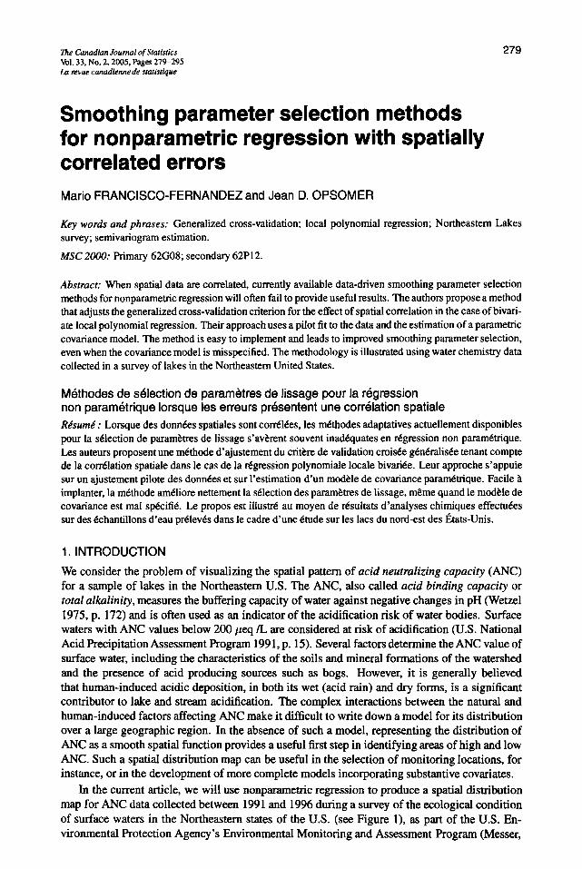
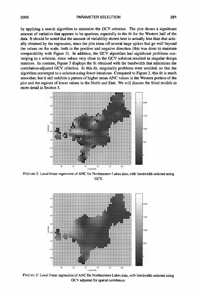
by applying a search algorithm to minimize the GCV criterion. The plot shows a significant amount of variation that appears to be spurious, especially in the fit for the Western half of the data. It should be noted that the amount of variability shown here is actually less than that actually obtained by the regression, since the plot trims off several large spikes that go well beyond the values on the scale, both in the positive and negative direction (this was done to maintain comparability with Figure 3). In addition, the GCV algorithm had significant problems con- verging to a solution, since values very close to the GCV solution resulted in singular design matrices. In contrast, Figure 3 displays the fit obtained with the bandwidth that minimizes the correlation-adjusted GCV criterion. In this fit, singularity problems were avoided, so that the algorithm converged to a solution using fewer iterations. Compared to Figure 2, this fit is much smoother, but it still exhibits a pattern of higher mean ANC values in the Western portion of the plot and the regions of lower values in the North and East. We will discuss the fitted models in more detail in Section 5 .

47

46

4s

U

f 3 43

42

41

40

78 76 74 72 m 68 LmJ-

FIGURE 2: Local linear regression of ANC for Northeastern Lakes data, with bandwidth selected using GCV.

47

46

4s

44

9 l 42

41

76 74 n m Lm/-

FIGURE 3: Local linear regression of ANC for Northeastern Lakes data, with bandwidth selected using GCV adjusted for spatial correlation.


The proposed smoothing parameter selection method will rely on estimating the correlation function and incorporating this estimate into the selection criterion. The idea of adjusting the selection criterion in this manner is not new. Altman (1990) discussed this approach for the time series case and referred to it as the “direct method” of bandwidth selection under correlation (the “indirect method” consists of transforming the residuals and then applying the unadjusted criterion to the transformed residuals). Related approaches are those of Chiu (1989) and Hart (1991). Other types of adjustments to the criterion that do not rely on explicitly incorporating the correlation function are also possible. Examples of such adjustments are the “leave 21+1 out” cross- validation approach (Hart & Vieu 1990) and the prediction-based cross-validation approach of Yao and Tong (1998). For references to other methods for bandwidth selection in this context, see Opsomer, Wang & Yang (2001).

The situation considered in this article is conceptually similar to that studied by these other authors. However, different methods are needed to estimate a correlation function in the spatial case. In particular, many methods that work well for observations that are equally spaced and lo- cated along a single dimension do not readily convert to the random-design, higher-dimensional case. Therefore, it is still of interest to study spatial smoothing separately from time series smoothing, and to develop a simple and practical bandwidth selection method for spatial smoothing.

The proposed bandwidth selection method requires estimation of the correlation function. We do this estimation by calculating the empirical semivariogram of the residuals of a pilot fit (see Cressie 1993, p. 70), and using a method-of-moments estimator for the parameters of the correlation function. In this context, we show that the binned empirical semivariogram can be viewed as a kernel regression estimator of the true semivariogram function, and prove its consistency under a version of increasing-domain asymptotics. This result is of some theoretical interest separately from the bandwidth selection context, since we did not find a previously published proof for the consistency of the binned semivariogram estimator.

The remainder of the paper is as follows. In Section 2, we describe the statistical model and the nonparametric estimator, and we explain the smoothing parameter selection method. Sec- tion 3 discusses estimation of the semivariogram and the parameters of the correlation function. In Section 4, simulation experiments evaluate the practical properties of our approach, and Sec- tion 5 discusses the application of the method to the Northeastern Lakes data.

2. SMOOTHING PARAMETER SELECTION WITH CORRELATION-ADJUSTED GCV

2. I . Review of local linear regression for spatial data.

Let {(Xi, x)}y=l be a set of RD+’-valued random vectors, where the Y, are scalar responses variables and the Xi are RD-valued predictor variables with a common density fz with compact support R & RD. The multivariate nonparametric regression problem is that of estimating m ( x ) = E(Y I X = z) at a location z E R, where m( ) is not restricted to belong to a specific parametric family of functions. In this article, we assume the model

Y,=m(Xi )+Ei , i = 1 , 2 ) . ” , n, (1)

where E ( ~ i I X i ) = 0, var(Ei I X i ) = u2, C O V ( E ~ , ~j I Xi, Xj) = u2pn(Xi - X j ) with pn(z) continuous, satisfying p,(O) = 1, pn(z) = p n ( - z ) , and Ipn(z)I 5 1, Vz. The subscript n in pn ( . ) allows for the correlation function to “shrink” as the sample size n -+ m. This will be made more precise below.

The local linear estimator for m( . ) at z is the solution for (Y to the least squares minimization


where H is a D x D symmetric positive definite matrix; K is a D-variate kernel and KH(u) = IHI-lK(H-lu). The bandwidth matrix H controls the shape and the size of the local neigh- borhood used for estimating m(z). The local linear estimator can be written explicitly as

%(z; H ) = eT(X,TW,X,)-'X,TW,Y = s;Y

where el is a length (D + 1) vector with 1 in the first entry and all other entries 0, X, is a matrix with ith row equal to (1, (Xi - z ) ~ ) , W , = diag {KH(X~ - z), . . . , K H ( X , - 2)). and

For the case of uncorrelated data with a random design, Ruppert & Wand (1994) derived the asymptotic mean squared error (AMSE) formula for the multivariate local linear estimator. Opsomer, Wang & Yang (2001) provide the corresponding results for D = 2 when the errors are correlated. Liu (2001) generalized those results to arbitrary D, and we briefly summarize those results below.

We introduce some notation. For any matrix B, we use X,,(B) and Xmin(B) to denote its maximum eigenvalue and minimum eigenvalue, respectively. Let 'flm(z) represent the Hessian matrix of a D-variate function m( - ) evaluated at z. Let X represent the sequence {XI, . . . , X,, . . .}. As commonly done in kernel regression, we will state all our results conditionally on K (see Ruppert & Wand 1994 for a discussion of this approach).

T Y = (Y1, ..., Y,) .

We require the following assumptions:

A1 The function m( - ) is second order differentiable on a compact set R, the error variance

A2 K( . ) is symmetric, Lipschitz continuous and s K ( u ) d u = 1, s uK(u) d u = 0 and

A3 The bandwidth matrix H is symmetric and positive definite. As n -+ 00, H -+ 0. The

A4 For the correlation function pn(. ), there exist constants pr, C, such that n s p,(u) du +

o2 > 0, and the design of the locations fi ( ) > 0 on R.

s uuTK(u) d u = pa(K)I with p 2 ( K ) # 0.

ratio X m , ( H ) / X m i n ( H ) is bounded above, and n l H I X 2 i n ( H ) -+ 00 as n -+ 00.

pr and n s Ipn(u)l d u 5 C,. For any sequence en > 0 satisfying nllD.z, -+ 00,

Assumption A4 implies that the integral of Ipn(z) l should vanish as n -+ 00, and the vanish- ing speed should not be slower than O( l/n). This assumption further implies that the integral of lpn(z)l is essentially dominated by the values of pa(%) near to the origin 0. Hence, the correlation is short-range and decreases as n + 00. Arguing somewhat loosely, this can be considered a case of increasing-domain spatial asymptotics (Cressie 1993, p. 100), since this setup can readily be transformed to one in which the correlation function pn is fixed with respect to the sample size, but the support fi for z expands. The current setup with fixed domain R and shrinking pn is more natural to consider when the primary purpose of the estimation is a fixed mean function m( ) defined over a spatial domain, not the correlation function itself.

Two examples of commonly used correlation functions that satisfy the conditions of assumption A4 for any D 2 1 are the exponential model

and the rational quadratic model

284 FRANCISCO-FERNANDEZ 8. OPSOMER Vol. 33, No. 2

with Q: > 0 in both cases (Cressie 1993, p. 61). Under assumptions Al-A4 and for x an interior point in R, Liu (2001) showed that

1 2 (4) E { 6 ( x ; H ) - m(z) I X} = - p 2 ( K ) tr(H23cm(z)) + op(tr(H2))

generalizing the results of Ruppert & Wand (1994) to the correlated error case. If we let AMSE(G(x; H ) ) denote the mean squared error approximation obtained by summing the lead- ing terms of the square of the bias (4) and of the variance (3, the asymptotically optimal local bandwidth matrix can be computed by minimizing AMSE(G(x; H ) ) with respect to H . As Liu (2001) showed, this minimizer is

where 3cm(x) if 3c,(z) is positive definite,

-3c,(z) if 3cm(z) is negative definite. ..Fi,(X) =

(If 3cm(z) is neither positive nor negative definite, the minimizer of AMSE(%(z; H ) ) might not exist, even if the minimizer for the mean squared error exists). Hence, the matrix ('6,(~))-'/~ determines the shape and the orientation of the local optimal bandwidth region, while the term before it determines its overall magnitude, which depends among other factors on the sample size n, on the dimension D of the covariate vector, and on the integrated correlation function p i . As in the independent error case, the optimal rate of convergence for the elements of H ( z ) is qn -1 / (D+4) ) .

The objective of most bandwidth selection methods is to obtain an estimator for the asyrnp- totically optimal global bandwidth, defined as the minimizer of

AMISE(H) = AMSE(G(z; H ) ) f ( z ) d ~ .

Unlike in the case of AMSE above, no closed form expression is available for the minimizer of AMISE. In the next section, we will propose a bandwidth selection criterion based on General- ized Cross-Validation and that is asymptotically equivalent to AMISE(H).

2.2. Bandwidth selection.

Consider selecting the bandwidth H that minimizes the GCV function

J

l n y, -Gi 1 - + ( S )

GCV(H) = - c( i=l

with S the n x n matrix whose ith row is equal to s$,, the smoother vector for x = Xi. Finding the minimizer of this function over the D(D + 1)/2 parameters in H can be performed using numerical algorithms as implemented in statistical software, or with a specialized procedure such as the one proposed by Kauermann and Opsomer (2003). However, we cannot use this criterion directly for selecting the bandwidth in the presence of correlated errors because its expectation is severely affected by the correlation. Specifically, as Liu (2001) showed, the GCV is asymptotically biased, in that

E {GCV(H) I X} = a2 + AMISE(H) -


Hence, when # 0, the correlation contributes a term to the expectation of the GCV criterion that depends on H and is of the same order as the variance component of AMISE(H) (see (5) ) , which is likely to lead to inappropriate bandwidth choices (see Section 4 for an evaluation of this effect in practice).

We propose to remove this effect by using the "bias-corrected" GCV criterion

with R the correlation matrix of the observations. Using the results of Liu (2001), it can be shown that CCV,(H) is conditionally asymptotically unbiased, in that

1 E{GCV,(H) I X} = u2 + AMISE(H) + oP (Xb,(H) + -).

nlHl Also, under the additional assumption that

GCV,(H) is consistent for AMISE(H) plus a term that does not depend on the bandwidth matrix H.

The criterion (7) is not yet a practical bandwidth selection criterion, since it requires knowl- edge of R. Therefore, we will assume a parametric form for the correlation function, say pn(. ; 8), and then replace the unknown R(8) in (7) by an estimate R(8). We write the "bias- corrected and estimated" GCV criterion as

How well (8) approximates (7) depends on whether the parametric form chosen for pn ( . ; 0) is appropriate, and how well 8 is estimated by 8. The former aspect will be discussed in Section 4, while the latter is addressed in the following result.

RESULT 1. Assume that the parametric form of pn( - ; 8) is correct, that p n ( . ; 8) is continuous and that its derivativefs) with respect to 8 are bounded. Assume also that H satisfies A3 and that there exists E > 0 such that 11 - tr(SR(0))I > E for all n. Under these assumptions,

GCVce(H) = GCV,(H) + Op(l18 - 811).

Under the stated assumptions, the result is immediate by an application of a first order Taylor series expansion for 6 = 8. The assumptions on pn(.; 8) are readily checked and hold for the exponential and rational quadratic models discussed above. While the assumption on : tr(SR(8)) appears restrictive, note that it is also required for the GCV criterion itself to be a well-defined bandwidth selector. In particular, too small values for the diagonal elements of H could lead to violation of this assumption and would result in instability in the GCV (or GCV,,) criterion. For a practical implementation of the GCV,,, we would recommend that the assumption be checked with 8 replaced by its estimate and only those values for H satisfying the condition be allowed in the search for the minimizer. Putting a lower bound on the allowable values of H is common practice in GCV implementations.

The immediate consequence of Result 1 is that as long as 8 can be estimated consistently, then GCV,,(H) is consistent for GCV,(H). Therefore, it is also consistent for AMISE(H) and a term that does not depend on H. In the next section, we discuss consistent estimators of the parameters of the correlation function for a specific function choice.


3. ESTIMATION OF THE CORRELATION FUNCTION

The bias-corrected GCV criterion relies on the parametric specification of the correlation function. In this article, we consider the isotropic exponential model given in (3), but the approach will hold more generally for other models, including those with anisotropy (correlation depending on direction as well as distance between observations) or nonzero nugget effects (local variability causing multiple Observations at the same location to be different from each other). The main requirement is that a parametric specification for the correlation function can be selected. We expect the exponential model to be broadly applicable for many spatial regression problems, since a positive correlation function that decreases smoothly in all directions very often provides a reasonable approximation for the observed spatial correlation. Because the focus of our approach is on estimating the mean function, not the correlation function, a high degree of accuracy in estimating the latter is not a prerequisite, and simple correlation models like the exponential will often suffice.

In order to estimate the spatial correlation function parameter(s) effectively, we express the correlation model as a semivariogram model and estimate that model by an empirical semivariogram. For correlation function (3), the unknown parameter B that needs to be estimated under the semivariogram formulation is ((T’, a) . We will construct simple estimators for both quanti- ties based on residuals E i from a pilot fit using local linear estimator (2) and a pilot bandwidth matrix &lot. The estimator for 0’ is defined as

. n

The estimator for a will be constructed from the empirical semivariogram

(see Cressie 1993, p. 69), with S ( d , t ) = {(i, j ) : d - t 5 llXi - Xjll < d + t } the set of all points that are at a distance d f t of each other, and n ( d , t ) the number of elements in S ( d , t ) . The number t > 0 is a tolerance value chosen to achieve a sufficient number of observations in S ( d , t ) . Under the assumptions made in this article, the empirical semivariogram +(.) estimates the semivariogram function -yn ( . ) = (T’ (1 - pn ( )).

The +(d) can be calculated for any distance d . Here, we propose to calculate +(d) for a grid of distances 0 < d l < dz < . . . < dJ+1, and estimate a by

where

(12)

Expression (12) is a method-of-moments estimator obtained by rewriting the correlation model (3) as a semivariogram model and solving for a. Estimators at a set of J lags d j are combined into (1 1) to improve the precision of the estimator. If a different correlation model than (3) is assumed, (12) will need to be replaced by a different corresponding expression. Alternatively, this simple estimation approach can be replaced by a more sophisticated one such as restricted maximum likelihoodor weighted least squares (Cressie 1993, p. 92).

The following results show that the estimators (9) and (10) are consistent. Proofs are in the Appendix.

1 G. - -(ln(&’) - ln(8’ - + ( d j ) ) , j = 1 , 2 , . . . , J. - nd j


RESULT 2. Assume that the 2, are obtainedfrom a pilotfit using local linear estimator ( 2 ) and a pilot bandwidth matrix Apilot. Let assumptions A l , A2 and A4 hold for the observations and the kernel, and let A3 hold afrer replacing H by Apilot. Then,

- 2 - 2 0 - (T +op(l).

RESULT 3. Let the assumptions of Result 2 hold, and assume the first two derivatives of the semivariogramfinction and the density of the observed distances exist. Assume E (&i&j&k) = 0 and cov(&i~j, EkEl) = COV(Ei, &k)COV(&j, ~ l ) + COV(E~, E~)COV(E~, &k) for all i , j , k , 1. Finally, assume that the tolerance value t satisfies t + 0, nt -+ co as n -+ 00. Then, for any d > 0,

%d) = m ( 4 + OP(1).

Result 3 shows that under the stated assumptions, the empirical semivariogram is a consistent estimator for the sernivariogram. The assumptions on the moments of ei are satisfied for the normal distribution and are made only to simplify the proof. They could be weakened and replaced by convergence bounds on moments of products of the errors, for instance. While the result is stated for +(d) which is a function of residuals from a pilot fit, it clearly also holds if the errors themselves are observed. Hence, it shows the consistency of the empirical semivariogram to the true sernivariogram for a stationary spatial random process. The method of proof in the Appendix treats the estimator q(d) as a kernel regression estimator with a uniform kernel K(d) = I{ldls1) and bandwidth parameter t. Using this approach resulted in a direct and simple proof of the consistency of the empirical semivariogram: after transforming the locations of the observations to polar coordinates, straightforward application of kernel asymptotics leads to the desired consistency. While we did not derive rates of convergence here, the same approach could certainly be used to do so.

COROLLARY 1. Under the assumptions of Result 3 and for anyfied J , we have

85 = a + op(l).

The corollary follows directly from Results 2 and 3 and the continuity of (12).

4. SIMULATION EXPERIMENTS In this section, a simulation study is carried out to evaluate the proposed bandwidth selection method. We compare criteria:

0 GCV(II), given in (6),

0 CCV,(H), corrected for the true correlation function and given in (7).

0 GCV,,(H), corrected using an estimated correlation function assuming that the errors follow an exponential correlation model, and given in (8).

For this purpose, 200 samples of size n = 400 are generated following regression model (l), where the design points Xi = (Xil, Xiz) are uniformly sampled in the unit rectangle, the mean function is the additive model m(X1, X Z ) = sin(2~X1) + 4(X2 - 0.5)2 and the random errors Ei are normally distributed with zero mean and exponential covariance function

(13) C O V ( E ~ , E ~ I Xi,Xj) = (r2exp{-allXi - x ~ I I ) ,


with u = 0.4. Several values of parameter a are considered: a = 5 (strong correlation), a = 20, a = 40 and a = 200 (approximately no correlation).

The local linear estimator (2) with Epanechnikov kernel

2 ~ ( x ) = -max{(l- l l ~ 1 1 ~ ) , 0 }

is used. For each simulated sample, we calculated the bandwidths obtained using the three GCV criteria, denoted by HGCV, HGCV~ and H G C V ~ ~ respectively. We will compare the methods based on their mean average squared error (MASE),

1 1 MASE(H) = -(Sm - m)t(Sm - m) + -02 tr(SRSt), n n

where m = (rn(Xl), rn(X2), . . . , rr~(X,))~ and R is the true correlation matrix of the errors. For comparison, we also computed Hopt, the minimizer of MASE(H). We implemented the local linear regression estimator as well as the GCV and corrected GCV procedures in Matlab 6.5.1 (code available upon request from the first author).

In the computation of H G C V ~ ~ , parameters u2 and a are estimated from nonparametric residuals obtained from a pilot fit with bandwidth Apilot = diag{&x, , &x2}, where ex,, &x2 denote the sample standard errors of the two components of the Xi. The distances d k = 0.001 + 2(k - l)t, k = 1,2,. . . ,30 with t = 0.005 are used in the empirical semivariogram.

lr

TABLE 1 : Simulation means of HGCV, H G C V ~ and H G C V ~ ~ and MASE-optimal bandwidth Hopt, for correctly specified correlation function.

- a HGCV

2o (0.099 0.016)

0.016 0.092

4o (0.101 0.001)

0.001 0.131

2oo (0.139 0.021)

0.021 0.255

Hopt

("y' 0.:73)

( "y5 0.:25)

0.150 -0.001 -0.001 0.296

0.140 -0.003

-0.003 0.264

Table 1 displays the MASE-optimal bandwidth Hopt and the simulation means of HGCV, HGCV~ and Hccvce as a function of a. When data are almost uncorrelated (a = 200), all three criteria produce similar bandwidths. The optimal bandwidth values increase as the correlation increases (a decreases). Bandwidths HGCV~ and H G C V ~ ~ track this behavior, while HGCV exhibits an oppositive behavior. For intermediate values of a, H G C V ~ ~ exhibits a slight tendency toward overestimation.

TABLE 2: Simulation means of MASE(H) corresponding to three bandwidth selection method and MASE(Hopt) for correctly specified correlation function. The numbers in parentheses are the simulation

standard errors.

a MASE(HGCV) MASE(HGCV~) ~ ( H G c v , , ) MASE(Hopt)

5 0.132 (0.002) 0.096 (0.006) 0.096 (0.006) 0.093

20 0.077 (0.002) 0.038 (0.002) 0.040 (0.005) 0.036

40 0.040 (0.007) 0.021 (0.001) 0.023 (0.002) 0.020 200 0.014 (0.001) 0.014 (0.001) 0.015 (0.001) 0.013


Table 2 shows the simulated MASE results corresponding to the three bandwidth selection methods and the minimum of MASE(H), i.e., MASE(HOpt). When we compare the methods based on their mean MASE values (Table 2), it is clear that H G C V ~ and HGCVce are close to fully efficient, while the performance of HGCV is unsatisfactory for values of a 5 40. The HGCVce are more variable than HGCV~, but still appear to provide a significant improvement over HGCV when correlation is present.

TABLE 3: Simulation means of HGCV. H G C V ~ , H G C V ~ ~ and Hopt for misspecified covariance function.

- - - b HGCV HGCV~ H G C V ~ ~ Hopt

160 (0.091 0.020) (0.174 0.001) (0.206 0.001) (0.: o.:63)

0.020 0.096 0.001 0.400 0.001 0.594

800 (0.090 0.015) (0.: 0 ) (0.: 0 ) ( 0 . 7 0 ) 0.015 0.088 0.336 0.564 0.327

We also considered the situation when the parametric covariance function is misspecified. The setup is the same as above, but the covariance model generating the errors follows the rational auadratic function:

U2

1 + bllXi - Xjtl12’ cQV(&i, &j I xi, Xj) =

where the dependence is controlled by parameter b. Two values of b are used: b = 160 and b = 800, corresponding to high and low levels of correlation. When estimating the covariances for the computation of HGCVce, misspecified model (13) is used, while H G C V ~ and Hopt use correct model (14).

Table 3 displays the average values of HGCV, H G C V ~ and HGCVce, as well as the optimal bandwidth. Table 4 shows the MASE results obtained using the bandwidths selected by three criteria, as well as MASE(Hopt). Although H G C V ~ ~ is not as successful as H G C V ~ in adjusting for the correlation and is more variable, both methods outperform HGCV. Hence, even in situations when the covariance model cannot be specified exactly, the corrected and estimated GCV criterion proposed in Section 2.2 can provide an improvement over completely ignoring spatial correlation. We expect our method to be robust to model misspecification as long as the Correlation can be reasonably well approximated by a positive and decreasing function of distance between observations, as is often observed in practice. For other correlation functions, for instance negative correlation or a positive correlation function with a large “bump” away from 0, the method is likely to be unsuccessful in obtaining a satisfactory bandwidth choice. This type of deviation from the assumed correlation model should be readily detectable in a plot of the empirical semivariogram.

TABLE 4: Simulation means of MASE(H) corresponding to three bandwidth selection methods and MASE(H,,t) for misspecified covariance function. The numbers in parentheses are the simulation

standard errors.

b MASE(HGCV) MASE(HGCV,) ~ ( H G C V ~ ~ ) MASE(Hopt)

160 0.116 (0.002) 0.070 (0.007) 0.078 (0.014) 0.066 800 0.083 (0.006) 0.035 (0.002) 0.047 (0.007) 0.034


5. EXAMPLE

We now return to the analysis of the Northeastern Lakes survey data. Some of the 338 sampled lakes had repeated measurements, so that the total number of recorded ANC values is 557 and ranged from -72.2 to 3,371 peqk. Latitude and longitude of each lake centroid were recorded in decimal degree units, and the goal of the analysis is to produce a spatial surface for the mean ANC over the region. Since we are not interested in the correlation structure of the data, we will not explicitly account for the fact that some lakes had multiple measurements and in particular, we will not include a nugget effect in the spatial correlation.

Figure 4 shows the locations of the ANC measurements and the grid of locations on which local linear estimates of the mean will be calculated. The estimation grid was constructed by overlaying the survey region with a 50 x 50 grid and then dropping every grid point that did not satisfy one of the following two requirements: (a) it is within 1.5 “grid cell lengths” from an observation point, or (b) the calculation for the estimate at that grid point uses a smoothing vector (2) that is sufficiently stable. This second requirement was determined by performing a pilot local linear fit with an initial bandwidth matrix Apilot = diag{6x,,,, 6xlong} = (1.445 0; 0 2.419) and evaluating the matrix inversion in (2) using the Matlab rcond() function, with values above 0.05 considered acceptable. Both requirements are admittedly somewhat arbitrary, but they represent a compromise between coverage over the region of interest and ability to avoid singular design matrices. The resulting set of estimation points covers the interior of the ANC measurement locations, except for the very sparse region in the Western comer, where some points in the interior of the ANC measurement locations were dropped. The inability to deal with data sparseness is a drawback of kernel-based smoothing methods such as local linear regression.

Using the pilot bandwidth Apilot as an initial value in the uncorrected GCV minimization procedure, the algorithm converged to

0.4067 0.001280 0.001280 1.024 H G G V =

The resulting mean ANC surface evaluated on the estimation grid is displayed in Figure 2. As mentioned in Section 1, HGCV is very close to the boundary of the feasible bandwidth region (“infeasible” bandwidths are defined here as those that lead to a singular matrix for at least one of the local linear estimators (2) at the estimation points). This close proximity to the boundary results in highly unstable fits and convergence problems for the algorithm. The range of mean ANC values obtained was from -26,3 10 to 32,065 peqk, well beyond the range of the data, and numerous local minima and maxima occur in the estimated mean function.

For the correlation-corrected method proposed in this paper, we used the exponential correlation model (13) from Section 4. A pilot local linear regression using Apilot was performed, resulting in parameter estimates 6 = 435.1 and 15 = 1.597. When comparing the empirical semivariogram values with the semivariogram function that results from using 6 and & in exponential model (13), we observed some non-random deviations between both sets of values. This could be due to the correlation of semivariogram estimates or to correlation model lack of fit. As discussed previously, however, precise estimation of the correlation function does not seem to be necessary for the purpose of correcting the GCV criterion, so that we proceeded with the exponential specification and these estimated values.

Starting from Apilot again, the corrected GCV minimization converged to

1 1.198 -0.000079 [ -0.OOOO79 1.787 H G C V c e =

and the resulting estimated mean ANC surface is shown in Figure 3. In order to rule out a local minimum, we also performed the corrected GCV minimization using HGCV as a starting value, but the algorithm converged to the same bandwidth value. Both the obtained HGCV and

2005 PARAMETER SELECTION 29 1

H G C V ~ ~ matrices have very small off-diagonal elements. We therefore repeated the bandwidth selection procedures constraining the bandwidths to be diagonal matrices to see if perhaps this might have an influence on the overall bandwidth selection method. The results were virtually identical to the ones reported above and will therefore not be discussed further.

r- -r .....

...... . o . . . . . . .o . p&:* 80 70 76 74 72 70 68 66

LMg-

FIGURE 4: Locations (in latituddongitude) of ANC measurements (0) and estimation grid (. ) for Northeastern Lakes survey.

The fit in Figure 3 is much smoother than that in Figure 2, with mean ANC values ranging from -369 to 2,387 peq/L. The extreme low and high values occur at the boundary of the estimation region, where smoothing methods such as local linear regression often result in unreliable estimates. The lowest values are outside the range of observed ANC values, making it likely these very low estimates are indeed spurious. The high peak around coordinate values (44,-76) appears real, however, with all the observed ANC values above 2,000 indeed occurring in that area. In contrast, the estimated mean ANC surface using HGCV displayed numerous local peaks above 2,000 that do not correspond to high observations.

In the analysis of ANC, the focus is most often on identifying areas where ANC values are low (200 peq/L). The fit in Figure 3 clearly shows regions of lower ANC in the North and East portions of the map. Those same regions are visible in Figure 2, but that is mainly because we "processed" this map to use the same scale as Figure 3, which involved trimming all the peaks and valleys that fell outside of the range of the scale. In fact, having both fits agree with respect to the general location of the low ANC areas within the study region is a further indication that the observed pattern is actually present in the data, not just induced by bandwidth choice. Overall, correcting for correlation appears to have produced an estimated mean ANC surface that is not only smoother and computationally more stable, but also effectively visualizes interesting patterns in the underlying data.

We performed several sensitivity analyses on the procedure and the obtained fit. First, we evaluated the effect of including a nugget effect in the correlation function. In the case of the exponential model, this implies that three parameters need to be estimated instead of two. The nugget effect is readily estimated from the repeated observations, and we adjusted the remaining parameter estimators accordingly. This had only a modest effect on the overall pilot fit. We obtained 3057.5 for the nugget effect, and the estimates for the remaining parameters were 6 = 431.6 and 6 = 1.528. After adjusting the GCV criterion for the correlation function with nugget effect and plugging in the parameter estimates, we obtained a new bandwidth matrix { 1.198 - 0.000159; -0.000159 1.796}, virtually indistinguishable from H G C V ~ ~ above.


Next, we wanted to investigate whether the correlation observed in the pilot fit residuals was in fact present in the data and not simply an artifact induced by our approach, since in the latter case, any dataset could potentially result in a substantial (and unwanted) GCV correction. To evaluate this, we performed a parametric bootstrap. We repeatedly resampled residuals from the fit obtained using H G C V ~ ~ and constructed bootstrap samples by randomly adding the resampled residuals to the model fits. Each bootstrap sample has approximately the same mean and variance function as the original dataset, but the errors are now spatially uncorrelated. We performed the pilot fit estimation of the correlation function parameters for each bootstrap sample, and the bootstrap mean value for the estimate of a was ii = 8.399, which indicates that a small amount of spatial correlation is indeed present in the residuals from the pilot smooth even when the true errors are uncorrelated. However, when this ii was used in the corrected GCV procedure, the bandwidth value obtained was (0.5625 - 0.000819; -0.000819 1.265}, close to HGCV which assumes uncorrelated errors. Using these bandwidth in the local linear regression produced an estimated mean ANC surface that is visually very similar to that in Figure 2.

Finally, we evaluated the sensitivity of the fitting procedure to the choice of the pilot bandwidth. To do this, we repeated the procedure with Apilot = 0.5 diag{6.x,a,,6~,o,,} and 2 diag{6x,a,, 6xlong}. The former pilot choice resulted in a bandwidth matrix H G C V ~ ~ with slightly smaller values than those described earlier, the latter in a bandwidth matrix with larger values. In both cases, the resulting fits were very similar but not identical to those shown in Figure 3, which is a further indication that the proposed procedure indeed captures and corrects for the presence of spatial correlation. A certain amount of sensitivity to prespecified “tuning parameters” like the pilot bandwidth is unavoidable in the application of nonparametric regression methods.

Pointwise confidence bands for the fit displayed in Figure 3 can in principle be computed. However, the correlation structure of the errors needs to be incorporated into these confidence bands for them to be reliable. Based on the assumed correlation model, the estimated variance of the %(Xi) can be computed by using the parameter estimates obtained from the variogram estimation on the residuals from the pilot fit. Alternatively, new parameter estimates can be computed by refitting the variogram on the residuals from the final fit, with this approach likely to be more reliable but would require additional computation effort. We do not explore this topic further here.

6. CONCLUSION In this article, we have proposed a simple GCV-based bandwidth selection method that is appropriate for smoothing spatial data when correlation is suspected. The method requires the computation of a pilot fit and the specification of a parametric correlation function, so that the method is not totally “model-free;” see Simonoff (1996, p. 167) for a discussion of why a fully nonparametric solution is not possible in this case. Nevertheless, the method appears reasonably robust to model misspecification, and works much better than completely ignoring the correlation and applying the traditional (unadjusted) GCV criterion. More generally, the approach described in this paper provides a framework for adjusting data-driven smoothing parameter selection methods in the spatial context and can easily be extended by incorporating other smoothing methods, more complicated correlation function estimation methods, or other optimality criteria.

We have demonstrated the applicability of the method on a dataset of ANC measurements for 338 lakes in the Northeastern U.S. In this data analysis, we showed that both the numerical stability of the algorithm and the resulting model fits improved dramatically after adjusting the bandwidth selection method for the presence of correlation, even when the spatial correlation function was imperfectly specified.


APPENDIX: PROOFS Proof of Result 2: Write

= Vn,l + Vn,2 + Vn,3* Using the ergodic theorem (Port 1994, Proposition 59.9), Vn,l + a2. Since the pilot bandwidth satisfies A3, (4) and ( 5 ) imply that

(15)

and hence, using a straightforwardextension of Result 5 of Fuller (1996, p. 300), Vn,2 = op(l). 0

Proof of Result 3: As in the proof of Result 2, write

E ( ( m ( x i ) - &(Xi; A p i l o t ) ) 2 I X) = op(l),

This immediately implies also that Vn,3 = op(l) by the S c h w a inequality.

1 c ( ( E i - Eli) - ( E j - ij))2 ?(d ) = - c (&a - E j ) 2 + - 1

2n(d, t , ( i , j ) E S ( d , t ) 2n(d, t , ( i , j ) E S ( d , t )

1 -- c (.i - Ej)((Ei - ti) - ( E j - El,)) n(d7 ( i , j )ES(d , t )

= y(d ) + 7n,2(4 + 7n,3(d), where ;j(d) is the empirical semivariogram of the errors. Since ~i - Eli = &(Xi; Apilot) - m(Xi) , wecanuse(15)andtheapproachoftheproofofResult2toshowthatTnYn,2(d), ~~,3(d) = op(l). Hence, the result will be established if we prove that for any fixed d > 0,

(16) E((=i(4 - m(4)"W = OP(1).

We rewrite q ( d ) as a Nadaraya-Watson estimator (see Wand & Jones 1995, p. 119)

where the kernel function K(d) is the indicator function I { ld l s1 } .

of y ( d ) separately. For the bias, we have To prove (16), we consider the bias and the variance components of the mean squared error

E (34 - m(4 I X)

A1 = 7 m -& (1 +o(l)) = OP(1)

by the differentiability assumptions for T,,( a ) . The convergence in this result follows after we show that E (A:) = o(1) and E (A2 - dfd(d))2 = o(l), where the expectation is now taken with respect to { X i , i = 1, . . . , n} and fd(. ) denotes the density of the distances. The summations in A: and (A2 - dfd(d))2 are over 4 indices, so that six cases need to be considered depending on which indices are taken to be equal. In all cases, a change to polar coordinates significantly simplifies the derivations:

Xi1 - X j l = rij C O s O i j ,

Xi2 - Xj2 = T i j sinOij,


so that llXi - Xj 1 1 = rij. The detailed calculations are omitted here.

where For the variance component of the mean squarederror in (16), write var(y(d) I X) = B1/B2,

n n n n

and

This is established by using the moment assumptions stated in Result 3, so that B1 can be written as the sum of nine terms, say E l l g r g = 1,. . . ,9 , containing covariance products. For each term, it can be shown that E (IB1,I) = o(1) (with respect to fz(. )), so that B1 = op(l) by a straightforward extension of Result 5 of Fuller (1996, p. 300). For B2, we can show that

0 E (B2 - d2f,j(d)2)2 = o(1) by using the same approach as for A2 above.

ACKNOWLEDGEMENTS

The research of M. Francisco-Ferngndez was partially supported by Grant PGIDIT03PXIC10505PN and MCyT Grant BFM2002-00265 (European FEDER support included). The work reported here was partially supported by STAR Research Assistance Agreements CR-829095 and CR-829096 awarded by the U.S. Environmental Protection Agency (EPA). This manuscript has not been formally reviewed by EPA. The views expressed here are solely those of the authors. EPA does not endorse any products or commercial services mentioned in this report. The authors thank Phil Larsen and Alan Herlihy of the EPA for their helpful explanation of ANC concepts, and the associate editor and two referees for constructive comments that improved the presentation of the article.

REFERENCES N. S. Altman (1990). Kernel smoothing of data with correlated errors. Journal of the American Statistical

Association, 85,749-759. S.-T. Chiu (1989). Bandwidth selection for kernel estimate with correlated noise. Statistics & Probability

Letters, 8,347-354. P. Craven & G. Wahba (1 979). Smoothing noisy data with spline functions: estimating the correct degree

of smoothing by the method of generalized cross-validation. Numerische Mathematik, 3 1,377-403. N. A. C. Cressie (1 993). Statistics for Spatial Data, Second edition. Wiley, New York. W. A. Fuller (1996). Introduction to Statistical Time Series, Second edition. Wiley, New York. T. C. Haas (1990). Lognormal and moving window methods of estimating acid deposition. Journal of the

J. D. Hart (1991). Kernel regression estimation with time series errors. Journal of the Royal Statistical

J. D. Hart (1 996). Some automated methods of smoothing time-dependent data. Journal of Nonparametric

J. D. Hart & P. Vieu (1990). Data-driven bandwidth choice for density estimation based on dependent data.

G. Kauermann & J. D. Opsomer (2003). Local likelihood estimation in generalized additive models. Scan-

D. P. Larsen, T. M. Kincaid, S. E. Jacobs & N. S. Urquhart (2001). Designs for evaluating local and regional

American Statistical Association, 85,950-963.

Sociefy Series B, 53, 173-187.

Statistics, 6, 115-142.

The Annals of Statistics, 18,873-890.

dinavian Journal of Statistics, 30,3 17-337.

scale trends. Bioscience, 51, 1049-1058.


X . Liu (2001). Kemel smoothing for spatially correlateddata. Ph. D. thesis, Department of Statistics, Iowa

J. J. Messer, R. A. Linthurst & W. S. Overton (1991). An EPA program for monitoring ecological status

J. D. Opsomer, Y. Wang & Y. Yang (2001). Nonparametxic regression with correlated errors. Statistical

S . C. Port (1994). Theorical Probability for Applications. John Wiley, New York. D. Ruppert & M. P. Wand (1994). Multivariate locally weighted least squares regression. Annals of Statis-

J. S . Simonoff (1996). Smoothing Methods in Statistics. Springer-Verlag, New York. U.S. National Acid Precipitation Assessment Program (1991). 1990 Integrated Assessment Report. Tech-

M. P. Wand & M. C. Jones (1995). KemelSmoothing. Chapman & Hall, London. R. G. Wetzel(l975). Limnology. W. B. Saunders Company, Philadelphia. Q. Yao & H. Tong (1 998). Cross-validatov bandwidth selections for regression estimation based on depen-

dent data. Journal of Statistical Planning and Inference, 68,387415.

State University.

and trends. Environmental Monitoring and Assessment, 17,67-78.

Science, 16, 134-153.

tics, 22,1346-1370.

nical report, Washington, DC., November 1991.

Received 4 June 2004 Accepted 20 October 2004

Mario FRANCISCO-FERNANDEZ: mariofrO udc.es Departamento de Matemdticas, Facultad de Infodt ica

Universidad de La Coruiia ES-1.5071 La Coruiia, Spain

Jean D. OPSOMER: jopsomerOiastate.edu Department of Statistics Ames, LA 50014, U.S.A.

Smoothing parameter selection methods for nonparametric ...

Documents

Transcript of Smoothing parameter selection methods for nonparametric ...