CONFIDENCE SETS FOR NONPARAMETRICWAVELET REGRESSION

By Christopher R. Genovese1and Larry Wasserman

2

Carnegie Mellon University

We construct nonparametric confidence sets for regression func-tions using wavelets. We consider both thresholding and modula-tion estimators for the wavelet coefficients. The confidence set isobtained by showing that a pivot process, constructed from theloss function, converges uniformly to a mean zero Gaussian pro-cess. Inverting this pivot yields a confidence set for the waveletcoefficients and from this we obtain confidence sets on functionalsof the regression curve.

August 21, 2002

1Research supported by NSF Grant SES 9866147.2Research supported by NIH Grants R01-CA54852-07 and MH57881 and NSF Grants

DMS-98-03433 and DMS-0104016.Key words and phrases: Confidence sets, Stein’s unbiased risk estimator, nonparametric

regression, thresholding, wavelets.

1

1 Introduction

Wavelet regression is an effective method for estimating inhomogeneous func-

tions. Donoho and Johnstone (1995a, 1995b, 1998) showed that wavelet re-

gression estimators based on nonlinear thresholding rules converge at the

optimal rate simultaneously across a range of Besov and Triebel spaces. The

practical implication is that, for denoising an inhomogeneous signal, wavelet

thresholding outperforms linear techniques. See for instance Cai (1999), Cai

and Brown (1998), Efromovich (1999), Johnstone and Silverman (2002), and

Ogden (1997). However, confidence sets for the wavelet estimators may not

inherit the convergence rate of function estimators. Indeed, Li (1989) shows

that uniform nonparametric confidence sets for regression estimators decrease

in radius at an n−1/4 rate. However, with additional assumptions, Picard and

Tribouley (2000) show that it is possible to get a faster rate for pointwise

intervals.

In this paper, we show how to construct uniform confidence sets for

wavelet regression. More precisely, we construct a confidence sphere in the

`2-norm for the wavelet coefficients of a regression function f . We use the

strategy of Beran and Dumbgen (1998), originating from an idea in Stein

(1981), in which one constructs a confidence set by using the loss function as

an asymptotic pivot. Specifically, let µ1, µ2, . . . be the coefficients for f in the

orthonormal wavelet basis φ1, φ2, . . ., and let (µ1, µ2, . . .) be corresponding

estimates that depend on a (possibly vector-valued) tuning parameter λ. Let

Ln(λ) =∑

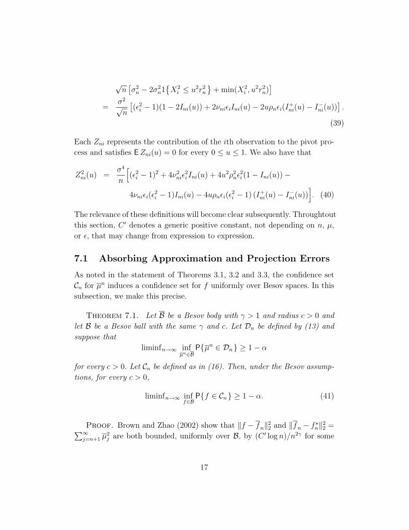
i(µi(λ) − µi)2 be the loss function and let Sn(λ) be an unbiased

estimate of Ln(λ). The Beran-Dumbgen strategy has the following steps.

1. Show that the pivot process Bn(λ) =√

n(Ln(λ) − Sn(λ)) converges

weakly to a Gaussian process with covariance kernel K(s, t).

2. Show that Bn(λn) also has a Gaussian limit, where λn minimizes Sn(λ).

This step follows from the previous step if λn is independent of the

pivot process or if Bn(λn) is stochastically very close to Bn(λn) for an

appropriate deterministic sequence λn.

3. Find a consistent estimator τ 2n of K(λn, λn).

2

4. Conclude that

Dn =

{µ :

Ln(λn) − Sn(λn)

τn/√

n≤ zα

}

=

{µ :

n∑`=1

(µn` − µ`)2 ≤ τn zα√

n+ Sn(λn)

}

is an asymptotic 1 − α confidence set for the coefficients, where zα

denotes the upper-tail α-quantile of a standard Normal and where

µn` ≡ µ`(λn).

5. It follows that

Cn =

{n∑

`=1

µ`φ`(·) : µ ∈ Dn

}is an asymptotic 1 − α confidence set for fn =

∑n`=1 µ`φ`.

6. With appropriate function-space assumptions, conclude that Cn is also

a confidence set for f .

The limit laws – and thus the confidence sets – we obtain are uniform

over Besov balls. The exact form of the limit law depends on how the µis are

estimated. We consider universal shrinkage (Donoho and Johnstone 1995a) ,

modulation estimators (Beran and Dumbgen 1998), and a restricted form of

SureShrink (Donoho and Johnstone 1995b).

Having obtained the confidence set Cn, we immediately get confidence

sets for any functional T (f). Specifically, (inff∈Cn T (f), supf∈CnT (f)) is an

asymptotic confidence set for T (f). In fact, if T is a set of functionals, then

the collection {(inff∈Cn T (f), supf∈CnT (f)) : T ∈ T } provides simultane-

ous intervals for all the functionals in T . If the functionals in T are point-

evaluators, we obtain a confidence band for f ; see Section 8 for a discussion of

confidence bands. An alternative method for constructing confidence bands

is given in Picard and Tribouley (2000).

In Section 2, we discuss the basic framework of wavelet regression. In

Section 3, we give the formulas for the confidence sets with known variance.

In Section 4, we extend the results to the unknown variance case. In Section

3

5, we describe how to obtain confidence sets for functionals. In Section 6, we

consider numerical examples. Finally, Section 7 contains technical results,

and Section 8 discusses a variety of related issues.

2 Wavelet Regression

Let φ and ψ be, respectively, a father and mother wavelet that generate the

following complete orthonormal set in L2[0, 1]:

φJ0,k(x) = 2J0/2φ(2J0x − k)

ψj,k(x) = 2j/2ψ(2jx − k),

for integers j ≥ J0 and k, where J0 is fixed. Any function f ∈ L2[0, 1] may

be expanded as

f(x) =2J0−1∑k=0

αk φJ0,k(x) +∞∑

j=J0

2j−1∑k=0

βj,k ψj,k(x) (1)

where αk =∫

fφJ0,k and βj,k =∫

fψj,k. For fixed j, we call βj· = {βj,k : k =

0, . . . , 2j − 1} the resolution-j coefficients.

Assume that

Yi = f(xi) + σεi, i = 1, . . . , n

where f ∈ L2[0, 1], xi = i/n, and εi are iid standard Normals. The goal is

to estimate f under squared error loss. We assume that n = 2J1 for some

integer J1. Let

fn(x) =2J0−1∑k=0

αk φJ0,k(x) +

J1∑j=J0

2j−1∑k=0

βj,k ψj,k(x) (2)

denote the projection of f onto the span of the first n basis elements.

Define empirical wavelet coefficients

αk =n∑

i=1

Yi

∫ i/n

(i−1)/n

φj0,k(x) dx ≈ 1

n

n∑i=1

φJ0,k(xi)Yi ≈ αk +σ√n

Zk

βj,k =n∑

i=1

Yi

∫ i/n

(i−1)/n

ψj,k(x) dx ≈ 1

n

n∑i=1

ψj,k(xi)Yi ≈ βj,k +σ√n

Zj,k,

4

where the Zks and Zj,ks are iid standard Normals. In practice, these coeffi-

cients are computed in O(n) time using the discrete wavelet transform.

We consider two types of estimation: soft thresholding and modulation.

The soft-threshold estimator with threshold λ ≥ 0, given by Donoho and

Johnstone (1995), is defined by

αk = αk (3)

βj,k = sign(βj,k) (|βj,k| − λ)+, (4)

where a+ = max(a, 0).

Two common rules for choosing the threshold λ are the universal thresh-

old and the SureShrink threshold. To define these, let σ2 be an estimate of σ2

and let ρn =√

2 log n. The universal threshold is λ = ρnσ/√

n. The levelwise

SureShrink rule chooses a different threshold λj for the nj = 2j coefficients

at resolution level j by minimizing Stein’s unbiased risk estimator (SURE)

with estimated variance. This is given by

Sn(λ) =σ2

n2J0 +

J1∑j=J0

S(λj) (5)

where

Sj(λj) =

nj∑k=1

[σ2

n− 2

σ2

n1{|βj,k| ≤ λj

}+ min(β2

j,k, λ2j)

], (6)

for J0 ≤ j ≤ J1. The minimization is usually performed over 0 ≤ λj ≤ρnj

σ/√

n, although we shall minimize over a smaller interval for reasons that

explain in the remark after Theorem 3.2. SureShrink can also be used to

select a global threshold by minimizing Sn(λ) using the same constant λ at

every level. We call this global SureShrink.

The second estimator we consider is the modulation estimator given by

Beran and Dumbgen (1998) and Beran (2000). Although these papers did

not explicitly consider wavelet estimators, we can adapt their technique to

construct estimators of the form

αk = ξφ αk (7)

βj,k = ξj βj,k, (8)

5

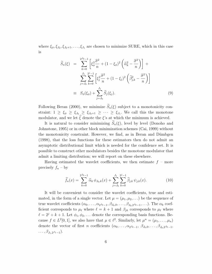
where ξφ, ξJ0 , ξJ0+1, . . . , ξJ1 are chosen to minimize SURE, which in this case

is

Sn(ξ) =2J0−1∑k=0

[ξ2φ

σ2

n+ (1 − ξφ)

2

(α2

k −σ2

n

)]+

J1∑j=J0

2j−1∑k=0

[ξ2j

σ2

n+ (1 − ξj)

2

(β2

j,k −σ2

n

)]

≡ Sφ(ξφ) +

J1∑j=J0

Sj(ξj). (9)

Following Beran (2000), we minimize Sn(ξ) subject to a monotonicity con-

straint: 1 ≥ ξφ ≥ ξJ0 ≥ ξJ0+1 ≥ · · · ≥ ξJ1 . We call this the monotone

modulator, and we let ξ denote the ξ’s at which the minimum is achieved.

It is natural to consider minimizing Sn(ξ), level by level (Donoho and

Johnstone, 1995) or in other block minimization schemes (Cai, 1999) without

the monotonicity constraint. However, we find, as in Beran and Dumbgen

(1998), that the loss functions for these estimators then do not admit an

asymptotic distributional limit which is needed for the confidence set. It is

possible to construct other modulators besides the monotone modulator that

admit a limiting distribution; we will report on these elsewhere.

Having estimated the wavelet coefficients, we then estimate f – more

precisely fn – by

fn(x) =2J0−1∑k=0

αk φJ0,k(x) +

J1∑j=J0

2j−1∑k=0

βj,k ψj,k(x). (10)

It will be convenient to consider the wavelet coefficients, true and esti-

mated, in the form of a single vector. Let µ = (µ1, µ2, . . .) be the sequence of

true wavelet coefficients (α0, . . . , α2J0−1, βJ0,0, . . . , βJ0,2J0−1, . . .). The αk coef-

ficient corresponds to µ` where ` = k + 1 and βjk corresponds to µ` where

` = 2j + k + 1. Let φ1, φ2, . . . denote the corresponding basis functions. Be-

cause f ∈ L2[0, 1], we also have that µ ∈ `2. Similarly, let µn = (µ1, . . . , µn)

denote the vector of first n coefficients (α0, . . . , α2J0−1, βJ0,0, . . . , βJ0,2J0−1,

. . . , βJ1,2J1−1).

6

For any c > 0 define:

`2(c) =

{µ ∈ `2 :

∞∑`=1

µ2` ≤ c2

},

and let Bςp,q(c) denote a Besov space with radius c. If the wavelets are r-

regular with r > ς, the wavelet coefficients of a function f ∈ Bςp,q(c) satisfy

||µ||ςp,q ≤ c, where

‖µ‖ςp,q =

∞∑j=J0

2j(ς+(1/2)−(1/p))

(∑k

|βj,k|p)1/p

q1/q

. (11)

Let

γ =

{ς p ≥ 2ς + 1

2− 1

p1 ≤ p < 2.

(12)

We assume that p, q ≥ 1 and also that γ > 1/2. However, for certain re-

sults we require the stronger condition that γ > 1. We also assume that the

mother and father wavelets are bounded, have compact support, and have

derivatives with finite L2 norms. We will call a space of functions f satisfy-

ing these assumptions a Besov ball with γ > 1/2 (or 1) and radius c and the

corresponding body of coefficients with ‖µ‖ ≤ c a Besov body with γ > 1/2

(or 1) and radius c. We use B to denote either, depending on context. If B is

a coefficient body, we will denote by Bm for any positive integer m, the set

of vectors (µ1, . . . , µm) for µ ∈ B.

3 Confidence Sets With σ Known

Here we give explicit formulas for the confidence set when σ is known. The

proofs are deferred until Section 7, and the σ unknown case is treated in

Section 4. It is to be understood in this section that σ replaces σ in (5) and

(9).

The confidence set is of the form

Dn =

{µn :

n∑`=1

(µ` − µ`)2dx ≤ s2

n

}. (13)

7

The definition of the radius sn is given in Theorems 3.1, 3.2, 3.3. In each

case, we will show that

limn→∞

supµn∈Bn

|P{µn ∈ Dn} − (1 − α)| = 0, (14)

for a coefficient body B. Strictly speaking, the confidence set Dn is for approx-

imate wavelet coefficients, but we show in Section 7 that the approximation

error can be easily accounted for. By the Parseval relation, Dn also yields a

confidence set for fn. We then show that if f is in a Besov ball B with γ > 1

and radius c then

lim infn→∞

inff∈B

P{f ∈ Cn} ≥ 1 − α (15)

where

Cn =

{f ∈ B :

∫ 1

0

(f(x) − fn(x))2 ≤ t2n

}(16)

and t2n = s2n+δ log n/n for any small, fixed δ > 0. The factor δ log n/n accom-

modates the difference between the true and approximate wavelet coefficients

and is negligible relative to the size of the confidence set.

Theorem 3.1 (Universal Threshold). Suppose that fn is the esti-

mator based on the global threshold λ = ρnσ/√

n. Let

s2n = σ2 zα√

n/2+ Sn(λ). (17)

Then, equations (14) and (15) hold for any Besov body B with γ > 1 and

radius c > 0.

Remark 3.1. When σ is known, this theorem actually holds with B =

`2(c) (and thus with Bn equal to a sphere of radius c in Rn) because there

is no need to prove asymptotic equicontinuity of the pivot process. However,

this generalization is not useful in practice.

We consider a restricted version of the SureShrink estimator where we

minimize SURE over %ρnσ/√

n ≤ λ ≤ ρnσ/√

n, where % > 1/√

2.

8

Theorem 3.2 (Restricted SureShrink). Let 1/√

2 < % < 1. In the

global case, let λJ0 = · · · = λJ1 ≡ λ be obtained by minimizing Sn(λ) over

%ρnσ/√

n ≤ λ ≤ ρnσ/√

n. In the levelwise case, let λ ≡ (λJ0 , . . . , λJ1) be

obtained by minimizing Sn(λJ0 , . . . , λJ1). Let

s2n = σ2 zα√

n/2+ Sn(λ). (18)

Then, equations (14) and (15) hold for any Besov body B with γ > 1 and

radius c > 0.

Remark 3.2. We conjecture that our results holds with only the restric-

tion that % > 0. We hope to report on this extension in a future paper.

Interestingly, the above theorem does not hold for % = 0 because the asymp-

totic equicontinuity of Bn fails, so some restriction on SureShrink appears to

be necessary.

Remark 3.3. The theorem also holds with a data-splitting scheme sim-

ilar to that used in Nason (1996) and Picard and Tribouley (2000), where we

use one half of the data to estimate the SURE-minimizing threshold and the

other half to construct the confidence set. In the case % > 1/√

2, this is not

required but it may be needed in the more general case % > 0.

Finally, we consider the modulation estimator.

Theorem 3.3 (Modulators). Let fn be the estimate obtained from

the monotone modulator. Let

s2n = τ

zα√n

+ S(a) (19)

where

τ 2 =2σ4

n

n∑`=1

(2ξ` − 1)2 + 4σ2

n∑`=1

(µ2

` −σ2

n

)2

(1 − ξ`)2 (20)

where ξ` is the estimated shrinkage coefficient associated with µ`. Then equa-

tion (14) holds for any Besov body B with γ > 1/2 and radius c > 0, and

equation (15) holds for any Besov body B with γ > 1 and radius c > 0.

9

4 Confidence Sets With σ Unknown

Suppose now that σ is not known. We consider two cases. The first, assumed

in Beran and Dumbgen (1998, eq. 3.2), is that there exists an independent,

uniformly consistent estimate of σ. For example, if there are replications

at each design point then the residuals at these points provide the required

estimator σ. More generally, letting L(·) denote the law of a random variable,

they assume the following condition:

(S1) There exists an estimate σ2n, independent of the empirical

wavelet coefficients, such that L(σ2n/σ

2) depends only on n and

such that

limn→∞

m(L(n1/2(σ2

n/σ2 − 1)), N(0, f2)

)= 0

where m(·, ·) metrizes weak convergence and f > 0.

In the absence of replication (or any other independent estimate of σ2),

we estimate σ2 by

σ2n = 2

n∑`=n

2+1

µ2` (21)

which Beran (2000) calls the high-component estimator. We then need to as-

sume that µn is contained in a more restrictive space. Specifically, we assume

the following:

(S2) The coefficients µ of f are contained in the set{µ ∈ `2(c) : ||βj·||2 ≤ ζj, j ≥ J2

}for some c > 0, J2 > J0 and some sequence of positive reals ζ =

(ζ1, ζ2, . . .) where ζj = O(2−j/2) and βj· denotes the resolution-j

coefficients.

Condition (S2) holds when f is in a Besov ball B with γ > 1/2. We note that

such a condition is implicit in Beran (2000) and Beran and Dumbgen (1998)

in the absence of (S1).

10

Beran and Dumbgen (1998) construct confidence sets with σ unknown by

including an extra term in the formula for s2n to account for the variability in

σ2n. This strategy is feasible for modulators since terms involving σ2

n separate

nicely in the estimated loss from the rest of the data. In thresholding estima-

tors, the empirical process in Theorem 7.2 depends on σn in a complicated

way, making it difficult to deal with σ separately. We offer two methods for

this case. For the soft-thresholded wavelet estimators, it turns out that a

plug-in method suffices. More generally, we can use “double confidence set”

approach.

For both approaches, we need the uniform consistency of σ.

Lemma 4.1. For any Besov body B with γ > 1/2,

supµ∈B

∣∣∣∣ σ2

σ2− 1

∣∣∣∣ P→ 0. (22)

The proof of this lemma is straightforward and is omitted.

In the plug-in approach, we simply replace σ by σ in the expressions of

the last section.

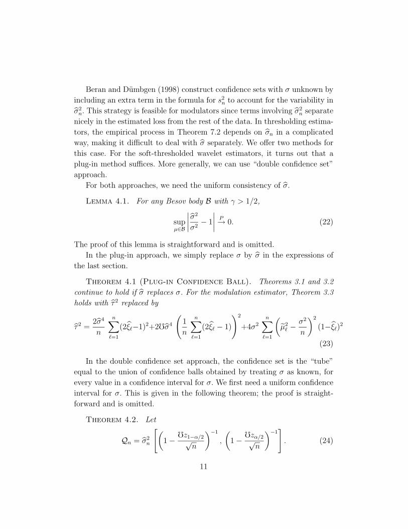
Theorem 4.1 (Plug-in Confidence Ball). Theorems 3.1 and 3.2

continue to hold if σ replaces σ. For the modulation estimator, Theorem 3.3

holds with τ 2 replaced by

τ 2 =2σ4

n

n∑`=1

(2ξ`−1)2+2fσ4

(1

n

n∑`=1

(2ξ` − 1)

)2

+4σ2

n∑`=1

(µ2

` −σ2

n

)2

(1−ξ`)2

(23)

In the double confidence set approach, the confidence set is the “tube”

equal to the union of confidence balls obtained by treating σ as known, for

every value in a confidence interval for σ. We first need a uniform confidence

interval for σ. This is given in the following theorem; the proof is straight-

forward and is omitted.

Theorem 4.2. Let

Qn = σ2n

[(1 − fz1−α/2√

n

)−1

,

(1 − fzα/2√

n

)−1]

. (24)

11

Under Condition (S1), we have

lim infn→∞

infσ>0

P{σ ∈ Qn} ≥ 1 − α. (25)

Under Condition (S2) with f = 2, we have for any Besov body B with γ > 1/2

lim infn→∞

infµ∈B,σ>0

P{σ ∈ Qn} ≥ 1 − α. (26)

Theorem 4.3 (Double Confidence Set). Let α = 1 −√

1 − α if

(S1) holds and let α = α/2 if (S2) holds. Let Qn be an asymptotic 1 − α

confidence interval for σ as in Theorem 4.2. Let

Dn =⋃

σ∈Qn

Dn,σ (27)

where Dn,σ is a 1− α confidence ball for µ from the previous section obtained

with fixed σ. Then,

lim infn→∞

infµn∈Bn

P{µn ∈ Dn} ≥ 1 − α. (28)

Finally, under conditions (S1) or (S2), Theorems 3.1, 3.2, and 3.3 continue

to hold with equation (28) replacing equation (14) and Dn as in equation

(27).

5 Confidence Sets for Functionals

Let f 7→ f ?n be the operation that takes f to the approximation defined in

equation (38). The reader can think of f ?n as simply the projection fn of f

onto the span of the first n basis functions. Define C?n to be the set of f ?

n

corresponding to coefficient sequences µn ∈ Dn. For real-valued functionals

T , define

J?n(T ) =

(inf

f?n∈C?

n

T (f ?n), sup

f?n∈Cn

T (f ?n)

). (29)

We then have the following immediately from the asymptotic coverage of

the confidence set.

12

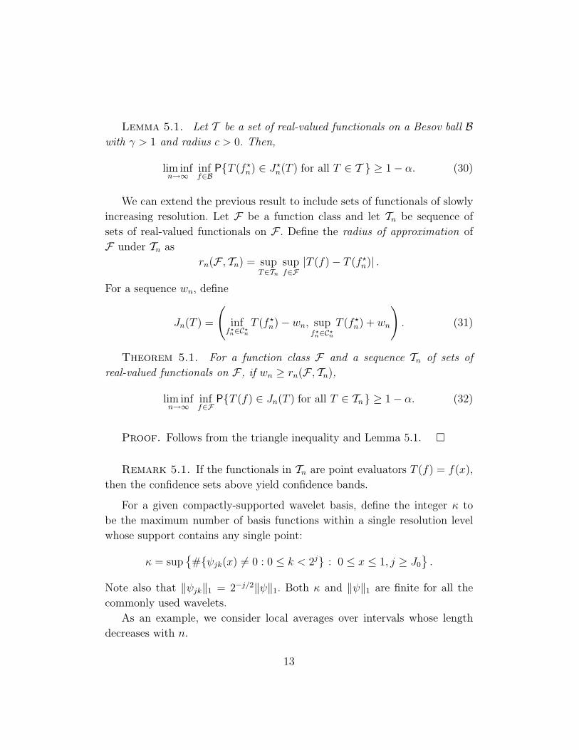
Lemma 5.1. Let T be a set of real-valued functionals on a Besov ball Bwith γ > 1 and radius c > 0. Then,

lim infn→∞

inff∈B

P{T (f ?n) ∈ J?

n(T ) for all T ∈ T } ≥ 1 − α. (30)

We can extend the previous result to include sets of functionals of slowly

increasing resolution. Let F be a function class and let Tn be sequence of

sets of real-valued functionals on F . Define the radius of approximation of

F under Tn as

rn(F , Tn) = supT∈Tn

supf∈F

|T (f) − T (f ?n)| .

For a sequence wn, define

Jn(T ) =

(inf

f?n∈C?

n

T (f ?n) − wn, sup

f?n∈C?

n

T (f ?n) + wn

). (31)

Theorem 5.1. For a function class F and a sequence Tn of sets of

real-valued functionals on F , if wn ≥ rn(F , Tn),

lim infn→∞

inff∈F

P{T (f) ∈ Jn(T ) for all T ∈ Tn} ≥ 1 − α. (32)

Proof. Follows from the triangle inequality and Lemma 5.1. ¤

Remark 5.1. If the functionals in Tn are point evaluators T (f) = f(x),

then the confidence sets above yield confidence bands.

For a given compactly-supported wavelet basis, define the integer κ to

be the maximum number of basis functions within a single resolution level

whose support contains any single point:

κ = sup{#{ψjk(x) 6= 0 : 0 ≤ k < 2j} : 0 ≤ x ≤ 1, j ≥ J0

}.

Note also that ‖ψjk‖1 = 2−j/2‖ψ‖1. Both κ and ‖ψ‖1 are finite for all the

commonly used wavelets.

As an example, we consider local averages over intervals whose length

decreases with n.

13

Theorem 5.2. Fix a decreasing sequence ∆n > 0 and define

Tn =

{T : T (f) =

1

b − a

∫ b

a

f dx, 0 ≤ a < b ≤ 1, |b − a| ≥ ∆n

}.

Let c > 0 and Fc =⋃

p,q≥1γ>1

Bςp,q(c).

If the mother and father wavelets are compactly supported with κ < ∞and ‖ψ‖1 < ∞ and if ∆−1

n = o(nζ/(log n)d) for some 0 ≤ ζ < 1 and d = 0

or for ζ = 1 and d > 0, then

rn(Fc, Tn) = o(nζ−1/(log n)d). (33)

Hence, for any sequence wn such that wn → 0 and wnn1−ζ(log n)d → ∞,

lim infn→∞

inff∈Fc

P{T (f) ∈ Jn(T ) for all T ∈ Tn} ≥ 1 − α. (34)

6 Numerical Examples

Here we study the confidence sets for the zero function f0(x) ≡ 0 and for the

two examples considered in Beran and Dumbgen (1998). We also compare

the wavelet confidence sets to confidence sets obtained from a cosine basis as

in Beran (2000).

The two functions, defined on [0, 1], are given by

f1(x) = 2(6.75)3x6(1 − x)3 (35)

f2(x) =

1.5 if 0 ≤ x < 0.30.5 if 0.3 ≤ x < 0.62.0 if 0.6 ≤ x < 0.80.0 otherwise.

(36)

Tables 1 and 2 report the results of a simulation using α = .05, n = 1024,

σ = 1, and 5000 iterations (which gives a 95% confidence interval for the

estimated coverage of length no more than 0.025). For comparison, the radius

of the standard 95 per cent χ2 confidence ball, which uses no smoothing, is

1.074. We used a symmlet 8 wavelet basis, and all the calculations were done

using the S+Wavelets package.

14

Table 1. Coverage and average confidence ball radius, by

method, in the σ-known case. Here, n = 1024 and σ = 1.

Method Function Coverage Average Radius

Universal f0 0.951 0.274f1 0.949 0.299f2 0.935 0.439

SureShrink (global) f0 0.946 0.270f1 0.941 0.292f2 0.937 0.401

SureShrink (levelwise) f0 0.944 0.268f1 0.940 0.289f2 0.927 0.395

Modulator (wavelet) f0 0.941 0.258f1 0.940 0.269f2 0.933 0.329

Modulator (cosine) f0 0.931 0.253f1 0.930 0.259f2 0.905 0.318

Table 2. Coverage, by thresholding method, in the σ-

unknown case using the Plug-in Confidence Ball. Again

n = 1024 and σ = 1.

Function Universal Sure GL Sure LW WaveMod CosMod

f0 0.961 0.955 0.954 0.955 0.999f1 0.963 0.955 0.953 0.961 0.999f2 0.938 0.940 0.929 0.951 0.997

15

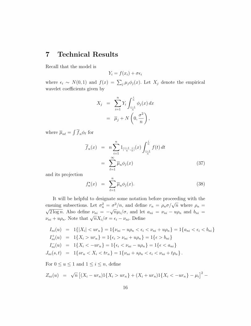
7 Technical Results

Recall that the model is

Yi = f(xi) + σεi

where εi ∼ N(0, 1) and f(x) =∑

j µjφj(x). Let Xj denote the empirical

wavelet coefficients given by

Xj =n∑

i=1

Yi

∫ in

i−1n

φj(x) dx

= µj + N

(0,

σ2

n

),

where µn` =∫

fnφ` for

fn(x) = n

n∑i=1

1[ i−1n

, in

](x)

∫ in

i−1n

f(t) dt

=∞∑

`=1

µnφj(x) (37)

and its projection

f ?n(x) =

n∑`=1

µnφj(x). (38)

It will be helpful to designate some notation before proceeding with the

ensuing subsections. Let σ2n = σ2/n, and define rn = ρnσ/

√n where ρn =√

2 log n. Also define νni = −√nµi/σ, and let ani = νni − uρn and bni =

νni + uρn. Note that√

nXi/σ = εi − νni. Define

Ini(u) = 1{|Xi| < urn} = 1{νni − uρn < εi < νni + uρn} = 1{ani < εi < bni}I+ni(u) = 1{Xi > urn} = 1{εi > νni + uρn} = 1{ε > bni}

I−ni(u) = 1{Xi < −urn} = 1{εi < νni − uρn} = 1{ε < ani}

Jni(s, t) = 1{srn < Xi < trn} = 1{νni + sρn < εi < νni + tρn} .

For 0 ≤ u ≤ 1 and 1 ≤ i ≤ n, define

Zni(u) =√

n[(Xi − urn)1{Xi > urn} + (Xi + urn)1{Xi < −urn} − µi

]2 −

16

√n

[σ2

n − 2σ2n1

{X2

i ≤ u2r2n

}+ min(X2

i , u2r2n)

]=

σ2

√n

[(ε2

i − 1)(1 − 2Ini(u)) + 2νniεiIni(u) − 2uρnεi(I+ni(u) − I−

ni(u))].

(39)

Each Zni represents the contribution of the ith observation to the pivot pro-

cess and satisfies E Zni(u) = 0 for every 0 ≤ u ≤ 1. We also have that

Z2ni(u) =

σ4

n

[(ε2

i − 1)2 + 4ν2niε

2i Ini(u) + 4u2ρ2

nε2i (1 − Ini(u)) −

4νniεi(ε2i − 1)Ini(u) − 4uρnεi(ε

2i − 1) (I+

ni(u) − I−ni(u))

]. (40)

The relevance of these definitions will become clear subsequently. Throughtout

this section, C ′ denotes a generic positive constant, not depending on n, µ,

or ε, that may change from expression to expression.

7.1 Absorbing Approximation and Projection Errors

As noted in the statement of Theorems 3.1, 3.2 and 3.3, the confidence set

Cn for µn induces a confidence set for f uniformly over Besov spaces. In this

subsection, we make this precise.

Theorem 7.1. Let B be a Besov body with γ > 1 and radius c > 0 and

let B be a Besov ball with the same γ and c. Let Dn be defined by (13) and

suppose that

liminfn→∞ infµn∈B

P{µn ∈ Dn} ≥ 1 − α

for every c > 0. Let Cn be defined as in (16). Then, under the Besov assump-

tions, for every c > 0,

liminfn→∞ inff∈B

P{f ∈ Cn} ≥ 1 − α. (41)

Proof. Brown and Zhao (2002) show that ‖f − fn‖22 and ‖fn − f ?

n‖22 =∑∞

j=n+1 µ2j are both bounded, uniformly over B, by (C ′ log n)/n2γ for some

17

universal c′ > 0. It then follows that

‖f − f ?n‖2

2 ≤(‖f − fn‖2 + ‖fn − f ?

n‖2

)2

≤ C ′ log n

n2γ.

Let

s2n = s2

n + δn =τ zα√

n+ δn + Sn

where δn = δ log n/n for some fixed, small δ > 0, and let W 2 = ‖fn − f ?n‖2

2.

Then,

‖fn − fn‖22 = ‖fn − f ?

n‖22 + ‖f ?

n − fn‖22

≤ W 2 +C log n

4n2γ,

uniformly over B. Hence,

P{‖fn − fn‖2

2 > s2n

}≤ P

{W 2 > s2

n − C log n

n2γ

}= P

{W 2 > s2

n + δn − C log n

4n2γ

}.

Now, uniformly,

lim infn→∞

δn − C log n

4n2γ> 0

since γ > 1 and so

lim supn→∞

supf∈B

P

{W 2 > s2

n + δn − C log n

4nγ/4

}≤ lim sup

n→∞supf∈B

P{W 2 > s2

n

}≤ α.

To do the same for f we note that

‖fn − f‖22 = ‖fn − f ?

n‖22 + ‖f − f ?

n‖22 + 2

⟨fn − f ?

n, f ?n − f

⟩= ‖fn − f ?

n‖22 + ‖f − f ?

n‖22 + 2

⟨fn − f ?

n, f ?n − fn

⟩= ‖fn − f ?

n‖22 + ‖f − f ?

n‖22 + 2

n∑i=1

(µ` − µ`)(µ` − µ`)

18

≤ ‖fn − f ?n‖2

2 + ‖f − f ?n‖2

2 + 2‖fn − f ?n‖2 ‖fn − f ?

n‖2

=(‖fn − f ?

n‖2 + ‖fn − f ?n‖2

)2

+ ‖f − fn‖22

≤(

W +

√C log n

4n2γ

)2

+C log n

4n2γ.

where the last inequality follows from the results in Brown and Zhao (2002)

since ‖fn − f ?n‖ ≤ ‖f − fn‖. Letting k2

n = C log n4n2γ , we have

P{‖f − fn‖2

2 > s2n

}≤ P

{(W + kn)2 > s2

n − k2n

}= P

{W 2 > s2

n − 2kn

√s2

n − k2n

}= P

{W 2 > s2

n + δn − 2kn

√s2

n + δn − k2n

},

where the first inequality follows from the non-negativity of W and kn and

is implied by W >√

s2n − k2

n − kn. Now, uniformly, since γ > 1,

lim infn→∞

δn − 2kn

√s2

n + δn − k2n > 0,

so

P{

W 2 > s2n + δn − 2kn

√s2

n + δn − k2n

}≤ lim sup

n→∞supf∈B

P{W 2 > s2

n

}≤ α.

¤

7.2 The Pivot Process

In the rest of this section, for convenience, we will denote µj simply by µj.

We now focus on the confidence set Dn for µn defined by

Dn =

{µn :

n∑i=1

(µi − µi)2 ≤ s2

n

}.

Our main task in showing that Dn has correct asymptotic coverage, is to

show that the pivot process has a tight Gaussian limit.

19

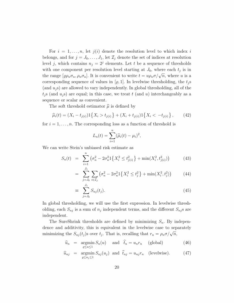
For i = 1, . . . , n, let j(i) denote the resolution level to which index i

belongs, and for j = J0, . . . , J1, let Ij denote the set of indices at resolution

level j, which contains nj = 2j elements. Let t be a sequence of thresholds

with one component per resolution level starting at J0, where each tj is in

the range [%ρnσn, ρnσn]. It is convenient to write t = uρnσ/√

n, where u is a

corresponding sequence of values in [%, 1]. In levelwise thresholding, the tjs

(and ujs) are allowed to vary independently. In global thresholding, all of the

tjs (and ujs) are equal; in this case, we treat t (and u) interchangeably as a

sequence or scalar as convenient.

The soft threshold estimator µ is defined by

µi(t) = (Xi − tj(i))1{Xi > tj(i)

}+ (Xi + tj(i))1

{Xi < −tj(i)

}, (42)

for i = 1, . . . , n. The corresponding loss as a function of threshold is

Ln(t) =n∑

i=1

(µi(t) − µi)2,

We can write Stein’s unbiased risk estimate as

Sn(t) =n∑

i=1

(σ2

n − 2σ2n1

{X2

i ≤ t2j(i)}

+ min(X2i , t2j(i))

)(43)

=

J1∑j=J0

∑i∈Ij

(σ2

n − 2σ2n1

{X2

i ≤ t2j}

+ min(X2i , t2j)

)(44)

≡J1∑

j=J0

Snj(tj). (45)

In global thresholding, we will use the first expression. In levelwise thresh-

olding, each Snj is a sum of nj independent terms, and the different Snjs are

independent.

The SureShrink thresholds are defined by minimizing Sn. By indepen-

dence and additivity, this is equivalent in the levelwise case to separately

minimizing the Snj(tj)s over tj. That is, recalling that rn = ρnσ/√

n,

un = argmin%≤u≤1

Sn(u) and tn = unrn (global) (46)

unj = argmin%≤uj≤1

Snj(uj) and tnj = unjrn (levelwise). (47)

20

We now define

Bn(u) =√

n (Ln(urn) − Sn(urn)) . (48)

We regard {Bn(u) : u ∈ U%} as a stochastic process. Let % > 1/√

2. In the

global case, we take U% = [%, 1]. In the levelwise case, we take U = [%, 1]∞,

the set of sequences (u1, . . . , uk, 1, 1, . . .) for any positive integer k and any

% ≤ uj ≤ 1. This process has mean zero because Sn is an unbiased estimate

of risk. The process Bn can be written as

Bn(u) =n∑

i=1

Zni(uj(i)), (49)

where Zni is defined in equation (39). For levelwise thresholding, Bn(u) is

also additive in the threshold components:

Bn(u) =

J1∑j=J0

Bnj(uj) =

J1∑j=J0

∑i∈Ij

Zni(uj). (50)

Each Bnj is of the same basic form as the sum of nj independent terms.

Lemma 7.1. Let B be a Besov body with γ > 1 and radius c > 0. The

process Bn(u) is asymptotically equicontinuous on U% uniformly over µ ∈ Bfor any % > 1/

√2 with both global and levelwise thresholding. In fact, it is

uniformly asymptotically constant in the sense that for all δ > 0,

lim supn→∞

supµ∈B

P∗

{sup

u,v∈U%

|Bn(u) − Bn(v)| > δ

}= 0. (51)

Proof. As above, let ani = νni−uρn and bni = νni +uρn. From equation

(39), we have for 0 ≤ u < v ≤ 1,

√n

2σ2(Zni(u) − Zni(v))

= (ε2i − 1)(Ini(v) − Ini(u)) − νniεi(Ini(v) − Ini(u))

−uρnεi(I+ni(u) − I−

ni(u)) + vρnεi(I+ni(v) − I−

ni(v))

21

= (ε2i − 1)1{uρn ≤ |εi − νni| < vρn} − νniεi1{uρn ≤ |εi − νni| < vρn}

−uρnεi1{uρn ≤ εi − νni < vρn} + uρnεi1{−vρn ≤ εi − νni < −uρn}+(v − u)ρnεi(I

+ni(v) − I−

ni(v))

= (ε2i − 1)1{uρn ≤ |εi − νni| < uρn + (v − u)ρn}

−bniεi1{bni < εi ≤ bni + (v − u)ρn} − aniεi1{ani − (v − u)ρn ≤ εi < ani}+(v − u)ρnεi [1{εi > bni + (v − u)ρn} − 1{εi < ani − (v − u)ρn}] (52)

From equation (52), we have that√

n

2σ2|Zni(u) − Zni(v)|

≤ (ε2i + (|νni| + uρn)|εi| + 1) 1{uρn ≤ |εi − νni| ≤ vρn} +

|v − u|ρn|εi|1{|εi − νni| > vρn}≤ (ε2

i + |νni||εi| + 1) 1{uρn ≤ |εi − νni| ≤ vρn} + ρn|εi|1{|εi − νni| ≥ uρn}≤ (ε2

i + |νni||εi| + 1) 1{%ρn ≤ |εi − νni| ≤ ρn} + ρn|εi|1{|εi − νni| ≥ %ρn}≡ ∆ni (53)

Let An0 = {1 ≤ i ≤ n : |νni| ≤ 1}, An1 = {1 ≤ i ≤ n : 1 < |νni| ≤ 2ρn},and An2 = {1 ≤ i ≤ n : |νni| > 2ρn}. The Besov condition implies that

n∑i=1

ν2nii

2γ ≤ C2n log n, (54)

so ν2nii

2γ ≤ C2n log n. Let n0(n) =⌈C1/γn1/2γ(log n)1/2γ

⌉. This is o(n) if

γ > 1/2 and o(√

n) if γ > 1. It follows that for i ≥ n0, |νni| ≤ 1; hence,

#(An0) = n − n0(n) and #(An1) + #(An2) ≤ n0(n).

From the above, we have in the global thresholding case that

sup%≤u≤v≤1

|Bn(u) − Bn(v)|

≤ sup%≤u≤v≤1

n∑i=1

|Zni(u) − Zni(v)|

≤ 2σ2

√n

n∑i=1

[(ε2

i + |νni||εi| + 1) 1{%ρn ≤ |εi − νni| ≤ ρn}

+ ρn|εi|1{|εi − νni| ≥ %ρn}]

(55)

22

We break the sum∑n

i=1 into three sums∑

i∈An0+

∑i∈An1

+∑

i∈An2and

consider these one at a time.

For the case where |νni| ≤ 1 we have the following:

2σ2

√n

∑i∈An0

[(ε2

i + |νni||εi| + 1) 1{%ρn ≤ |εi − νni| ≤ ρn} + ρn|εi|1{|εi − νni| ≥ %ρn}]

≤ 2σ2

√n

∑i∈An0

(ε2i + (1 + ρn)|εi| + 1) 1{|εi| ≥ %ρn − 1} .

Let tn = %ρn − 1. By equations (67) and (68), the expected value of each

summand is

E(ε2i + (1 + ρn)|εi| + 1

)1{|εi| ≥ %ρn − 1}

= 2(tn + ρn + 1)φ(tn) + 4(1 − Φ(tn))

= o(n−1/2).

The entire sum thus goes to zero as well. To see the last equality, note that

there exists δ > 0 such that

φ(tn) =1√2π

exp

{−1

2t2n

}=

1√2πe

e−%2ρ2n/2 e%ρn

=1√2πe

n√

2%√log n

−%2

= o(n−1/2−δ),

because√

2%√log n

− %2 < −1/2 − δ for large enough n, where δ = |%2 − 1/2|/2.

It follows that ρnφ(tn) = o(n−1/2) and similarly for (1 − Φ(tn)) ∼ φ(tn)/tn.

For the case where 1 < |νni| ≤ 2ρn we have the following:

2σ2

√n

∑i∈An1

[(ε2

i + |νni||εi| + 1) 1{%ρn ≤ |εi − νni| ≤ ρn} + ρn|εi|1{|εi − νni| ≥ %ρn}]

≤ 2σ2

√n

∑i∈An1

(ε2i + 3ρn|εi| + 1) 1{|εi − νni| ≥ %ρn} .

The expected value of each summand is bounded by 2 + 3ρn. The expected

value of the entire sum is thus bounded by

n0(n)√n

2σ2(2 + 3ρn) → 0,

23

because γ > 1 implies n0(n)ρn/√

n → 0.

For the case where 2ρn < |νni| we have the following from equation (53):

2σ2

√n

∑i∈An2

[(ε2

i + |νni||εi| + 1) 1{%ρn ≤ |εi − νni| ≤ ρn} + ρn|εi|1{|εi − νni| ≥ %ρn}]

≤ 2σ2

√n

( ∑i∈An2

(ε2i + 2ρn|εi| + 1) +

∑i∈An2

(|νni| − ρn)|εi|1{|εi| ≥ |νni| − ρn})

.

The expected value of the summands in the first term is bounded by 2+2ρn.

The expected value of the summands in the second term is bounded by

2(|νni| − ρn)φ(|νni| − ρn). Hence, the expected value of the entire sum is

bounded by

n0(n)√n

2σ2(2 + ρn + 2(|νni| − ρn)φ(|νni| − ρn)) → 0,

because γ > 1 implies n0(n)ρn/√

n → 0.

We have shown that E sup%≤u≤v≤1 |Bn(u)−Bn(v)| → 0. The result follows

for all δ > 0 by Markov’s inequality.

Next, consider the levelwise thresholding case. The product space U% =

[%, 1]∞ is the set of sequences (u1, . . . , uk, 1, 1, . . .) over positive integers k

and % ≤ uj ≤ 1. By Tychonoff’s theorem, this space is compact and thus

totally bounded, so U% is totally bounded under the product metric d(u, v) =∑∞`=J0

2−`|u` − v`|. For u ∈ U∞, define

Bn(u) =n∑

i=1

Zni(uj(i)).

It follows then that for any u, v ∈ U∞, d(u, v) ≤ 1 − % and

|Bn(u) − Bn(v)| ≤n∑

i=1

∣∣Zni(uj(i)) − Zni(vj(i))∣∣ (56)

≤n∑

i=1

supu,v∈U%

|Zni(u) − Zni(v)| (57)

≤n∑

i=1

∆ni, (58)

24

where ∆ni is the u, v independent bound established above in equation (53).

The result above shows that

E supu,v∈U%

|Bn(u) − Bn(v)| → 0. (59)

This implies that Bn is asymptotically constant (and thus equicontinuous)

on U%. ¤

Lemma 7.2. Let B be a Besov body with γ > 1 and radius c > 0.

For any fixed u1, . . . , uk in either global or levelwise thresholding, the vector

(Bn(u1), . . . , Bn(uk)) converges in distribution to a mean zero Gaussian on

Rk, uniformly over µ ∈ B, in the sense that

supµ∈B

m(L(Bn(u1), . . . , Bn(uk)), N(0, Σ(u1, . . . , uk; µ)) → 0,

where m is any metric on Rk that metrizes weak convergence and where Σ

represents a limiting covariance matrix, possibly different for each µ.

Proof. We begin by showing that the Lindeberg condition holds uni-

formly over µ ∈ B and over 0 ≤ u ≤ 1.

First consider global thresholding. Define ||Zni|| = sup0≤u≤1 |Zni(u)|. Re-

call that E Zni = 0 for all n and i. Now by equations (39) and (40),

Z2ni(u) ≤ 2σ4

n

[(ε2

i − 1)2 + 4u2ρ2nε

2i (1 − Ini(u)) + 4ν2

niε2i Ini(u)

]≡ ℵ1 + ℵ2 + ℵ3.

Note that none of ℵ1,ℵ2 or ℵ3 depend on u. Hence,

||Zni||21{||Zni|| > η} ≤ (ℵ1 + ℵ2 + ℵ3)1{(ℵ1 + ℵ2 + ℵ3) > η2

}≤

3∑r=1

3∑s=1

ℵrJs (60)

where Js = 1{ℵs > η2/3}. We will now show that the nine terms in (60) are

exponentially small in n which implies that the Lindeberg condition holds.

Moreover, we will see that the condition holds uniformly over `2(c).

25

First,

P

{ℵ1 >

η2

3

}= P

{|ε2

i − 1| >η√

n

σ2√

12

}≤ 2 exp

{− η

√n

8σ2√

12

}using the fact that P{|χ2

1 − 1| > t} ≤ 2e−t(t∧1)/8. To bound ℵ2 we use Mill’s

ratio:

P

{ℵ2 >

η2

3

}≤ P

{|εi| >

η

σrn

√48

}≤ 2

rn

√48

ηe−η2/(96r2

n) = 2ρ√

48

η√

ne−nη2/(96ρ2).

For the third term, if µi = 0, ℵ3 = 0. If µi 6= 0,

P

{ℵ3 >

η2

3

}≤ P

({|Xi| ≤ rn} ∩

{ε2i >

η2

48σ2µ2i

})≡ b(µi).

An elementary calculus argument shows that b(µi) ≤ b(µ∗) where

|µ∗| =ρnσ

2√

n+

1

2

√ρ2

nσ2

n+

4η√48n

.

Now, for all large n,

b(µ∗) ≤ P{ε > −ρnσ +

√n|µ∗|

}≤ P

{ε >

n1/4√η

6

}≤ 6

η√

2πn1/4e−η

√n/72.

These inequalities show that for η > 0 and for s = 1, 2, 3, E Jsi ≤K1 exp(−K2 min(η, η2)

√n). Because

√Eℵ2

1i ≤ K3/n,√

Eℵ22i ≤ ρ2

nK4/n,

and√

Eℵ23i ≤ µ2

i K5, the Cauchy-Schwarz and equation (60) show that for

η > 0,

En∑

i=1

‖Zni‖21{‖Zni‖ > η} ≤ K6(σ, ρ, c) exp(−K7(σ, ρ) min(η, η2)√

n). (61)

Here, the constants Kj depend at most on σ. It follows that the Lindeberg

condition holds uniformly by applying the Cauchy-Schwartz inequality to

(60).

26

Write Bn(u) ≡ Bn;µ(u) to emphasize the dependence on µ and similarly

for Zni;µi(u). In particular, let Bn;0(u) denote the process with µ1 = µ2 =

· · · 0. Let Ln;µ(u) denote the law of Bn;µ(u) =∑n

i=1 Zni;µi(u) and let N denote

a Normal with mean 0 and variance 2. By the triangle inequality,

m(Ln;µ(u),N ) ≤ m(Ln;0(u),N ) + m(Ln;µ(u),Ln;0(u))

where m(·, ·) denotes the Prohorov metric. By the uniform Lindeberg condi-

tion above, the CLT holds for Ln;0(u) and hence, by Theorem 7.3, m(Ln;0(u),N ) →0. Now we show that

supµ∈B

m(Ln;µ(u),Ln;0(u)) → 0. (62)

Note that√

n

2σ2|Zni;µi

(u) − Zni;0(u)|

=∣∣∣(ε2

i − 1)(Ini;µi(u) − Ini;0(u)) + νniεiIni;µi

(u)

−uρnεi[(I+ni;µi

(u) − I+ni;0(u)) − (I−

ni;µi(u) − I−

ni;0(u))]∣∣∣

This can be bounded as in the proof of Lemma 7.1 and the sum split over

the same three cases |νni| ≤ 1, 1 < |νni| ≤ 2ρn, and |νni| > 2ρn. It follows

that

supµ∈B

E sup%≤u≤1

|Bn;µ(u) − Bn;0(u)| ≤ a2n (63)

where an → 0; note that an does not depend on u or µ. Therefore,

supµ∈B

sup%≤u≤1

P{|Bn;µ(u) − Bn;0(u)| > an} ≤ a2n

an

= an

for all large n. Recall that, by Strassen’s theorem, if P{|X − Y | > ε} ≤ ε

then the marginal laws of X and Y are no more than ε apart in Prohorov

distance. Hence,

supµ∈B

sup%≤u≤1

m(Ln;µ(u),Ln;0(u)) ≤ an → 0. (64)

27

This establishes the theorem for one u. When Bn(u1, . . . , uk) is an Rk-valued

process for some fixed k,

E ‖Bn;µ(u1, . . . , uk) − Bn;0(u1, . . . , uk)‖ ≤ k E sup%≤u≤1

|Bnr;µ(u) − Bnr;0(u)| ,

(65)

so by equation (63) the sup of the former is bounded by ka2n. Since k is fixed,

the result follows. Thus, (62) holds for any finite dimensional marginal.

The same method shows that the result also holds in the levelwise case.

¤

Theorem 7.2. For any Besov body with γ > 1 and radius c > 0 and for

any 1/√

2 < % < 1, there is a mean zero Gaussian process W such Bn à W

uniformly over µ ∈ B, in the sense that

supµ∈B

m(L(Bn),L(W )) → 0, (66)

where m is any metric that metrizes weak convergence on `∞[%, 1].

Proof. The result follows from the preceeding lemmas in both the global

and levelwise cases. Lemmas 7.3 and 7.2 shows that the finite-dimensional

distributions of the process converge to Gaussian limits. Lemma 7.1 proves

asymptotic equicontinuity. It follows then that Bn converges weakly to a tight

Gaussian process W . ¤

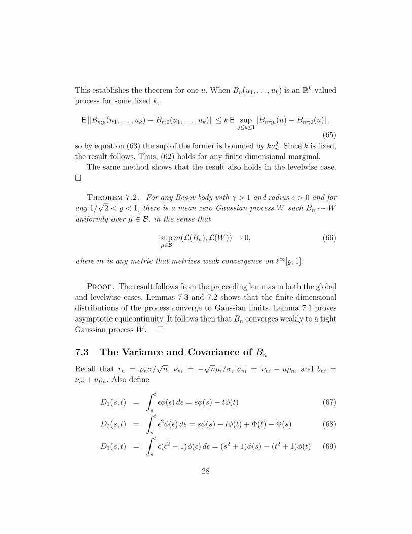
7.3 The Variance and Covariance of Bn

Recall that rn = ρnσ/√

n, νni = −√nµi/σ, ani = νni − uρn, and bni =

νni + uρn. Also define

D1(s, t) =

∫ t

s

εφ(ε) dε = sφ(s) − tφ(t) (67)

D2(s, t) =

∫ t

s

ε2φ(ε) dε = sφ(s) − tφ(t) + Φ(t) − Φ(s) (68)

D3(s, t) =

∫ t

s

ε(ε2 − 1)φ(ε) dε = (s2 + 1)φ(s) − (t2 + 1)φ(t) (69)

28

D4(s, t) =

∫ t

s

(ε2 − 1)2φ(ε)dε

= 2 (Φ(t) − Φ(s)) + s(s2 + 1)φ(s) − t(t2 + 1)φ(t). (70)

Let Kn(u, v) = Cov (Bn(u), Bn(v)). It follows from equation (40) that

Kn(u, u) = E Z2ni(u)

=2σ4

n

[1 + 2ν2

niD2(ani, bni) + 2u2ρ2n (1 − D2(ani, bni)) −

2νniD3(ani, bni) + 2uρn (D3(−∞, ani) − D3(bni,∞))]

=2σ4

n

[1 + 2u2ρ2

n + 2anibniD2(ani, bni) −

2bni(a2ni + 1)φ(ani) + 2ani(b

2ni + 1)φ(bni)

]=

2σ4

n

[1 + 2u2ρ2

n + 2anibni

(Φ(bni) − Φ(ani)

)+

2bnia2niφ(ani) − 2anib

2niφ(bni) −

2bni(a2ni + 1)φ(ani) + 2ani(b

2ni + 1)φ(bni)

]=

2σ4

n

[1 + 2u2ρ2

n + 2anibni

(Φ(bni) − Φ(ani)

)︸ ︷︷ ︸I

+

II︷ ︸︸ ︷2aniφ(bni) − 2bniφ(ani)

]≡ 2σ4

n

[1 + I + II

].

Theorem 7.3. Let B be a Besov ball with γ > 1/2 and radius c > 0.

Then,

limn→∞

supµ∈B

∣∣∣∣∣n∑

i=1

E Z2ni(u) − 2σ4

∣∣∣∣∣ = 0.

Proof. Apply Lemma 7.4 to the sum of terms I and II. This is of the

form 1n

∑ni=1 gn(νni), where

gn(x) = 2u2ρ2n + 2(x2 − u2ρ2

n)(Φ(x + uρn) − Φ(x − uρn)) +

29

2(x − uρn)φ(x + uρn) − 2(x + uρn)φ(x − uρn).

We have gn(0) → 0 because |gn(0)| ≤ 6ρnn−%2

, and hence n > 288/ε implies

that |gn(0)| < ε.

Now, if |x| > 2ρn, then by Mill’s inequality, |gn(x)| ≤ Cρ2n. If |x| ≤ 2ρn,

the same holds because each term is of order ρ2n. Hence, ‖gn‖∞ = O(log n).

For x in a neighborhood of zero,

|gn(x) − gn(0)| ≤ |g′n(ξ)| |x| for some |ξ| ≤ |x|

≤ sup|ξ|≤|x|

|g′n(ξ)| |x|.

Hence,

supn

|gn(x) − gn(0)| ≤ |x| supn

sup|ξ|≤|x|

|g′n(ξ)|.

By direct calculation, for ε > 0 and δ = min(ε, 1/8), sup|ξ|≤|x| |g′n(ξ)| ≤ 1,

so |x| ≤ δ implies supn |gn(x) − gn(0)| ≤ ε. Thus (gn) is an equicontinuous

family of functions at 0.

By Lemma 7.4, the result follows. ¤

Lemma 7.3. Let B be a Besov body with γ > 1/2 and radius c > 0.

Then the function Kn(u, v) = Cov (Bn(u), Bn(v)) converges to a well defined

limit uniformly over µ ∈ B:

limn→∞

supµ∈B

∣∣Kn(u, v) − 2σ4∣∣ = 0.

Proof. Theorem 7.3 proves the result for u = v. Let 0 ≤ u < v ≤ 1.

Then, by equation (39)

Zni(u)Zni(v) =σ4

n(ε2 − 1)2(1 − 2Ini(v) + 2Ini(u)) +

2σ3

√n

ε(ε2 − 1){

vrnI−ni(v) + urnI−

ni(u) − µi −

vrnI+ni(v) − urnI+

ni(u) + 3µIni(u) +

2urnJni(u, v) − 2urnJni(−v,−u)}

+

2σ2ε2{2µ2Ini(u) + 2urn(µ + rnv)Jni(u, v) +

2urn(vrn − µv)Jni(−v,−u)}.

30

Let ani = νni − vρ and bni = νni + vρ. We then have

Kn(u, v) = E (Zni(u)Zni(v))

=2σ4

n

[1 − D4(ani, bni) + D4(ani, bni)

vρnD3(−∞, ani) + uρnD3(−∞, ani) + νni −

vρnD3(bni,∞) − uρnD3(bni,∞) − 3νniD3(ani, bni)

2uρnD3(bni, bni) − 2uρnD3(ani, ani) +

2ν2niD2(ani, bni) + 2uvρn(ρn − νni)D2(bni, bni) +

2uvρn(ρn + νni)D2(ani, ani)].

The proof that this converges is essentially the same as the proof of Theorem

7.3. ¤

Lemma 7.4. Let B be a Besov ball with γ > 1/2. Let gn be a sequence

of functions equicontinuous at 0, with ‖gn‖∞ = O((log n)α) for some α > 0,

and satisfying gn(0) → a ∈ R. Then,

limn→∞

supµ∈B

1

n

n∑i=1

gn(µi

√n) = a.

Proof. Without loss of generality, assume that a = 0. Let Mn = ‖gn‖∞.

Fix ε > 0. By equicontinuity, there exists δ > 0 such that |x| < δ implies

|gn(x) − gn(0)| < ε/4 for all n. By assumption, there exists an N such that

|gn(0)| < ε/4 for n ≥ N . Since B is by assumption a Besov ball, there is a

constant C such that for all n,∑n

i=1 µ2i i

2γ ≤ C2 log n, for all µ ∈ B. See (Cai

1999, pp. 919–920) for inequalities that imply this.

Let νni = µi

√n. The condition on µ implies for all n that

n∑i=1

ν2nii

2γ ≤ C2n log n.

31

Let the set of such νns be denoted by Bn. We thus have

supµ∈B

∣∣∣∣∣ 1nn∑

i=1

g(µi

√n)

∣∣∣∣∣ ≤ supνn∈Bn

1

n

n∑i=1

|g(νni)| .

Let n0 =⌈C1/γn1/2γ(log n)1/2γ/δ1/γ

⌉. This is less than n and bigger than

N for large n. Then for i ≥ n0 and n ≥ N , |νni| ≤ δ and |gn(νni)| ≤ ε/2. We

have

1

n

n∑i=1

|gn(νni)| ≤ n0

nMn +

ε

2

n − n0 + 1

n

≤ n−(1−1/2γ) (log n)1/2γ C1/γMn

δ2+

ε

2.

Thus, as soon as

n (log n)−1

2γ−1 ≥(

C1/γ

δ1/γmax

(1,

2Mn

ε

)) 2γ2γ−1

,

we have

supνn∈Bn

1

n

n∑i=1

|gn(νni)| ≤ ε,

which proves the lemma. ¤

7.4 Proofs of Main Theorems

Proof Theorem 3.1. This follows from Theorems 7.2, and 7.3. The last

statement follows from Theorems 7.1. ¤

Proof Theorem 3.2. This follows from Theorems 7.2, 7.3, and the

fact that B(u) = B(1) + oP (1), uniformly in % ≤ u ≤ 1 and µ ∈ B. The last

statement follows from Theorems 7.1. ¤

Proof Theorem 3.3. This follows from the Theorem 3.2 in Beran and

Dumbgen (1998) and Theorem 7.1. ¤

32

Proof Theorem 4.1. Let m = σ/σ The pivot process with σ “plugged

in” is

Bn(u) =√

n

n∑i=1

[(µi − µi(urnm))2 +

[mσ2

n − 2mσ2n1

{X2

i ≤ u2r2nm2

}+ min(X2

i , u2r2nm

2)]]

= Bn(um) + (m2 − 1)σ2

n

n∑i=1

(1 − 2

{|βj,k| ≤ urnm

})= Bn(u) + oP (1),

uniformly over u ∈ U% and µ ∈ B, by Lemmas 7.1 and 4.1. The result follows.

¤

Proof Theorem 4.3. Let µ0 and σ0 denote the true values of µ and

σ, respectively. Then under (S1) we have,

P{µn0 ∈ Dn} ≥ P{σ0 ∈ Qn}P{µn

0 ∈ Dn | σ0 ∈ Qn}≥ P{σ0 ∈ Qn}P{µn

0 ∈ Dn,σ0 | σ0 ∈ Qn}= P{σ0 ∈ Qn}P{µn

0 ∈ Dn,σ0 } .

Hence,

lim infn→∞

infµn∈Bn

P{fn ∈ Dn} ≥ (1 − α)2 = (1 − α).

Under (S2),

P{µn0 6∈ Dn} = P{µn

0 6∈ Dn, σ0 /∈ Qn} + P{µn0 6∈ Dn, σ0 ∈ Qn}

≤ P{σ0 /∈ Qn} + P{µn0 6∈ Dn,σ0 , σ0 ∈ Qn}

≤ P{σ0 /∈ Qn} + P{µn0 6∈ Dn,σ0 } .

Thus,

lim infn→∞

infµn∈Bn

P{fn ∈ Cn} ≥ (1 − α − α) = 1 − α.

This completes the proof.

33

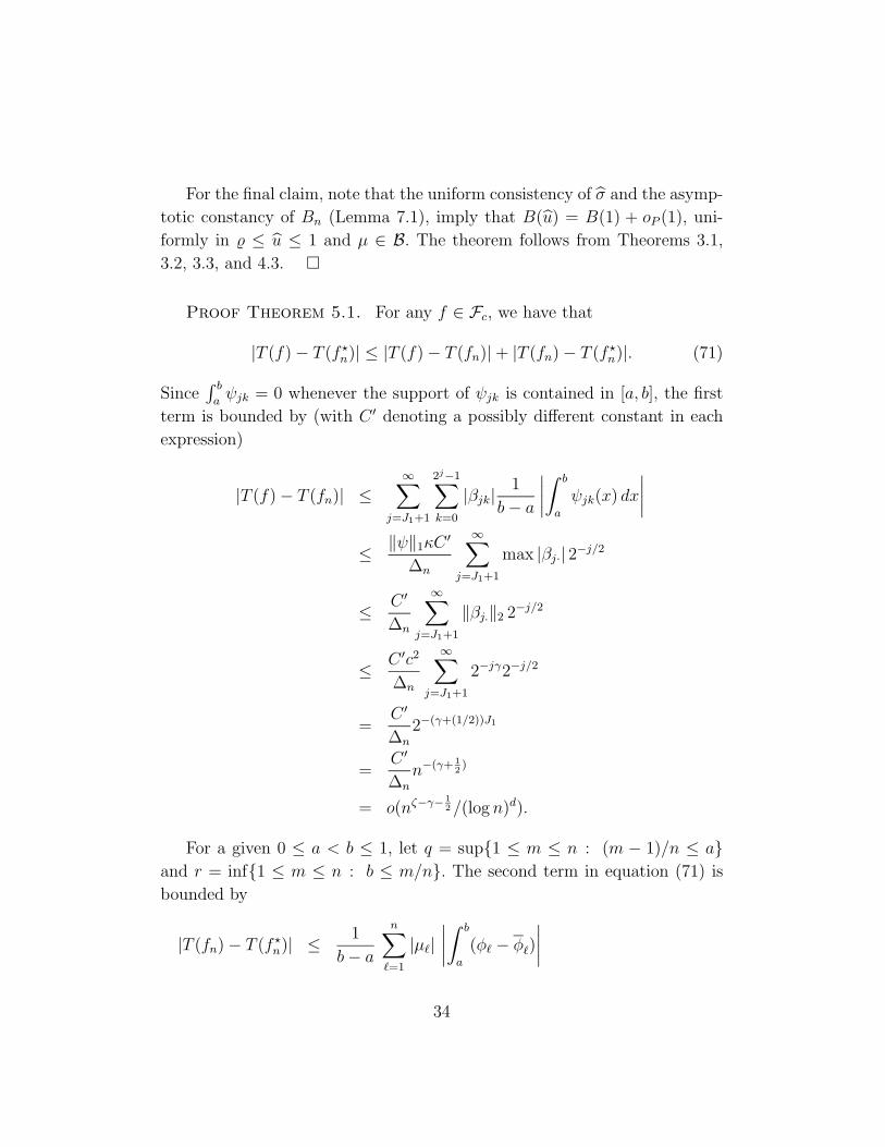
For the final claim, note that the uniform consistency of σ and the asymp-

totic constancy of Bn (Lemma 7.1), imply that B(u) = B(1) + oP (1), uni-

formly in % ≤ u ≤ 1 and µ ∈ B. The theorem follows from Theorems 3.1,

3.2, 3.3, and 4.3. ¤

Proof Theorem 5.1. For any f ∈ Fc, we have that

|T (f) − T (f ?n)| ≤ |T (f) − T (fn)| + |T (fn) − T (f ?

n)|. (71)

Since∫ b

aψjk = 0 whenever the support of ψjk is contained in [a, b], the first

term is bounded by (with C ′ denoting a possibly different constant in each

expression)

|T (f) − T (fn)| ≤∞∑

j=J1+1

2j−1∑k=0

|βjk|1

b − a

∣∣∣∣∫ b

a

ψjk(x) dx

∣∣∣∣≤ ‖ψ‖1κC ′

∆n

∞∑j=J1+1

max |βj·| 2−j/2

≤ C ′

∆n

∞∑j=J1+1

‖βj.‖2 2−j/2

≤ C ′c2

∆n

∞∑j=J1+1

2−jγ2−j/2

=C ′

∆n

2−(γ+(1/2))J1

=C ′

∆n

n−(γ+ 12)

= o(nζ−γ− 12 /(log n)d).

For a given 0 ≤ a < b ≤ 1, let q = sup{1 ≤ m ≤ n : (m − 1)/n ≤ a}and r = inf{1 ≤ m ≤ n : b ≤ m/n}. The second term in equation (71) is

bounded by

|T (fn) − T (f ?n)| ≤ 1

b − a

n∑`=1

|µ`|∣∣∣∣∫ b

a

(φ` − φ`)

∣∣∣∣34

=1

b − a

n∑`=1

|µ`|∣∣∣∣∣∫ b

a

φ` −∫ r/n

(q−1)/n

φ`

∣∣∣∣∣≤ 1

b − a

n∑`=1

|µ`|(∫ a

(q−1)/n

|φ`| +∫ r/n

b

|φ`|)

≤ 1

b − a

2J0−1∑k=0

|αk|C0

n+

4κC1

n

J1∑j=J0

max |βj·|2j/2

≤ 1

b − a

2J0−1∑k=0

|αk|C0

n+

4κC1

n

J1∑j=J0

‖βj·‖22j/2

≤ 1

b − a

2J0−1∑k=0

|αk|C0

n+

4κC1c

n

J1∑j=J0

2−(γ− 12)j

=

1

b − a

2J0−1∑k=0

|αk|C0

n+

4κC ′1c

n+ 4κC ′′

1 c 2−(γ+ 12)J1

≤ 1

b − a

[C0c2

J0

n+

4κC ′1c

n+ 4κC ′′

1 c 2−(γ+ 12)J1

]=

1

b − a

[C ′

n+ C ′ n−(γ+ 1

2)

]≤ 1

∆n

[C ′

n+ C ′ n−(γ+ 1

2)

]= o(nζ−1/(log n)d).

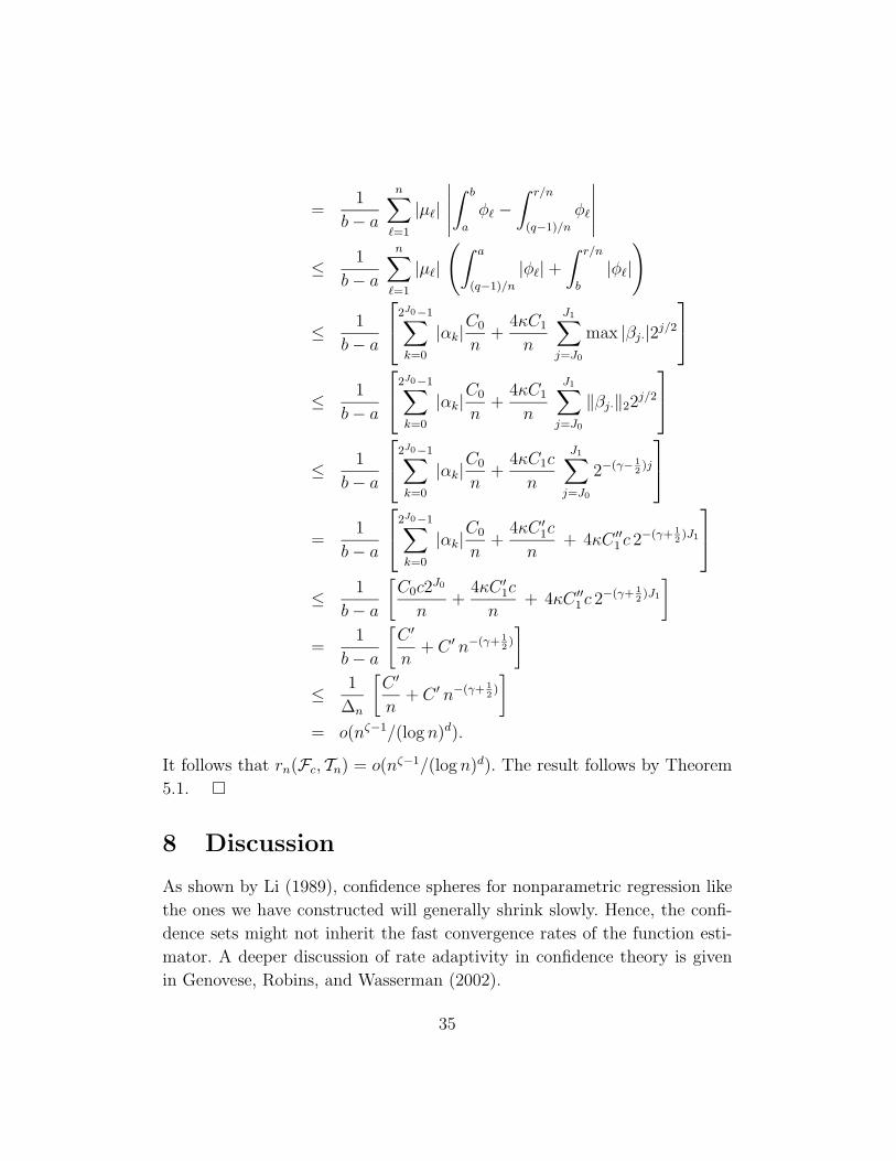
It follows that rn(Fc, Tn) = o(nζ−1/(log n)d). The result follows by Theorem

5.1. ¤

8 Discussion

As shown by Li (1989), confidence spheres for nonparametric regression like

the ones we have constructed will generally shrink slowly. Hence, the confi-

dence sets might not inherit the fast convergence rates of the function esti-

mator. A deeper discussion of rate adaptivity in confidence theory is given

in Genovese, Robins, and Wasserman (2002).

35

We have chosen to emphasize confidence balls and simultaneous confi-

dence sets for functionals. A more traditional approach is to construct an

interval of the form f(x)±wn where f(x) is an estimate of f(x) and wn is an

appropriate sequence of constants. This corresponds to taking T (f) = f(x),

the evaluation functional, in Theorem 5.1. There is a rich literature on this

subject; a recent example in the wavelet framework is Picard and Tribouley

(2000). Such confidence intervals are pointwise in two senses. First, they fo-

cus on the regression function at a particular point x, although they can

be extended into a confidence band. Second, the validity of the asymptotic

coverage usually only holds for a fixed function f : the absolute difference be-

tween the coverage probability and the target 1−α converges to zero for each

fixed function, but the supremum of this difference over the function space

need not converge. Moreover, in this approach one must estimate the asymp-

totic bias of the function estimator or eliminate the bias by undersmoothing.

While acknowledging that this approach has some appeal and is certainly of

great value in some cases, we prefer the confidence ball approach for several

reasons. First, it avoids having to estimate and correct for the bias which is

often difficult to do in practice and usually entails putting extra assumptions

on the functions. Second, it produces confidence sets that are asymptoti-

cally uniform over large classes. Third, it leads directly to confidence sets

for classes of functionals which we believe are quite useful in scientific ap-

plications. Of course, we could take the class of functionals T to be the set

of evaluation functions f(x) and so our approach does produce confidence

bands too. It is easy to see, however, that without additional assumptions on

the functions these bands are hopelessly wide. We should also mention that

another approach is to construct Bayesian posterior intervals as in Barber,

Nason, and Silverman (2002) for example. However, the frequentist coverage

of such sets is unknown.

In Section 5, we gave a flavor of how information can be extracted from

the confidence ball Cn using functionals. Beran (2000) discusses a different

approach to exploring Cn which he calls “probing the confidence set.” This

involves plotting smooth and wiggly representatives from Cn. A generalization

of these ideas is to use families of what we call parametric probes. These are

parameterized functionals tailored to look for specific features of the function

36

such as jumps and bumps. In a future paper, will report on probes as well as

other practical issues that arise. In particular, we will report on confidence

sets for other shrinkage schemes besides thresholding and linear modulators.

References

Barber, S., Nason, G. and Silverman, B. (2002). Posterior probability

intervals for wavelet thresholding. J. Royal Statist. Soc. Ser. B, 64, 189–205.

Beran, R. (2000). REACT scatterplot smoothers: superefficiency through

basis economy. J. Amer. Statist. Assoc. 95, 155–171.

Beran, R. and Dumbgen, L. (1998). Modulation of estimators and con-

fidence sets. Ann. Statist. 26, 1826–1856.

Brown, L. and Zhao, L. (2001). Direct asymptotic equivalence of non-

parametric regression and the infinite dimensional location problem. Techni-

cal report, Wharton School.

Cai, T. (1999). Adaptive wavelet estimation: a block thresholding and or-

acle inequality approach. Ann. Statist. 27, 898–924.

Cai, T. and Brown, L. (1998). Wavelet shrinkage for non-equispaced

samples. Ann. Statist. 26, 1783–1799.

Donoho, D. and Johnstone, I. (1995a). Adapting to unknown smooth-

ness via wavelet shrinkage. J. Amer. Statist. Assoc. 90, 1200–1224.

Donoho, D. and Johnstone, I. (1995b). Ideal spatial adaptation via

wavelet shrinkage. Biometrika 81, 425–455.

Donoho, D. and Johnstone, I. (1998). Minimax Estimation via Wavelet

Shrinkage. Annals of Statistics 26, 879–921.

Efromovich, S., (1999). Quasi-linear Wavelet Estimation, Journal of the

37

American Statistical Association, 94, 189–204.

Genovese, C., Robins, J. and Wasserman, L. (2002). Wavelets and

adaptive inference. In progress.

Johnstone, I. and Silverman, B. (2002). Risk bounds for Empirical

Bayes estimates of sparse sequences, with applications to wavelet smoothing.

Unpublished manuscript.

Li, K. (1989). Honest confidence regions for nonprametric regression. Ann.

Statist. 17, 1001–1008.

Ogden, R. T. (1997). Essential Wavelets for Statistical Applications and

Data Analysis. Birkhauser, Boston.

Picard, D. and Tribouley, K. (2000). Adaptive confidence interval for

pointwise curve estimation. Ann. Statist. 28, 298–335.

Stein, C. (1981). Estimation of the mean of a multivariate normal distri-

bution. Ann. Statist. 9, 1135–1151.

38