Logic of Confidence

Noname manuscript No.(will be inserted by the editor)

Logic of Confidence

Pavel Naumov · Jia Tao

the date of receipt and acceptance should be inserted later

Abstract The article studies knowledge in multiagent systems where dataavailable to the agents may have small errors. To reason about such uncertainknowledge, a formal semantics is introduced in which indistinguishability re-lations, commonly used in the semantics for epistemic logic S5, are replacedwith metrics to capture how much two epistemic worlds are different from anagent’s point of view. The main result is a logical system sound and completewith respect to the proposed semantics.

Keywords Uncertainty · Confidence of Knowledge · Axiomatic System

1 Introduction

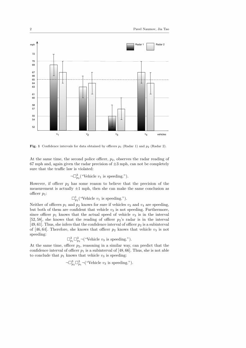
Uncertainty about information in multiagent systems often comes from theimprecision in measurements or small errors in data. Consider an example ofthe radar data about four different vehicles depicted in Figure 1. The data isreported by two different police officers. The first police officer, p1, observesvehicle v1 going with speed 69 miles per hour (mph). Assuming that the pre-cision of the radar is ±3 mph, officer p1 concludes that the actual speed ofvehicle v1, in miles per hour, is in the interval [66, 72]. Such an interval is oftenreferred to as a confidence interval. Since driving a vehicle at any speed in thisinterval exceeds 65 mph speed limit, officer p1 concludes that the driver ofvehicle v1 breaks the traffic law, as long as the precision of the radar is indeed±3 mph. We write it formally as

�3p1

(“Vehicle v1 is speeding.”).

Pavel NaumovMcDaniel College, Westminster, Maryland 21157, USAE-mail: [email protected]

Jia TaoBryn Mawr College, Bryn Mawr, Pennsylvania 19010, USAE-mail: [email protected]

2 Pavel Naumov, Jia Tao

65

69

63

66

60

72

61

64

58

70

67

v1 v2 v3 v4

mph

vehicles

57

55

Radar 1 Radar 2

54

52

Fig. 1 Confidence intervals for data obtained by officers p1 (Radar 1) and p2 (Radar 2).

At the same time, the second police officer, p2, observes the radar reading of67 mph and, again given the radar precision of ±3 mph, can not be completelysure that the traffic law is violated:

¬�3p2


However, if officer p2 has some reason to believe that the precision of themeasurement is actually ±1 mph, then she can make the same conclusion asofficer p1:

�1p2


Neither of officers p1 and p2 knows for sure if vehicles v2 and v4 are speeding,but both of them are confident that vehicle v3 is not speeding. Furthermore,since officer p1 knows that the actual speed of vehicle v3 is in the interval[52, 58], she knows that the reading of officer p2’s radar is in the interval[49, 61]. Thus, she infers that the confidence interval of officer p2 is a subintervalof [46, 64]. Therefore, she knows that officer p2 knows that vehicle v3 is notspeeding:

�3p1�3

p2¬(“Vehicle v3 is speeding.”).

At the same time, officer p2, reasoning in a similar way, can predict that theconfidence interval of officer p1 is a subinterval of [48, 66]. Thus, she is not ableto conclude that p1 knows that vehicle v3 is speeding:

¬�3p2�3

p1¬(“Vehicle v3 is speeding.”).

Logic of Confidence 3

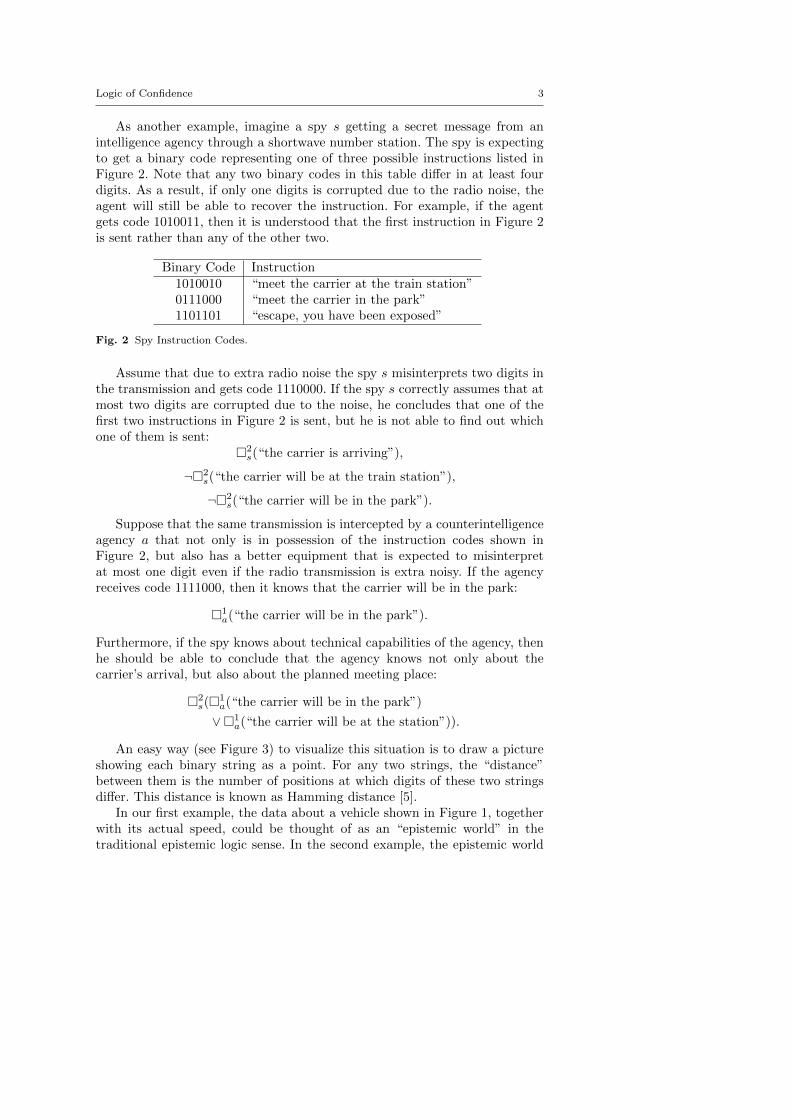
As another example, imagine a spy s getting a secret message from anintelligence agency through a shortwave number station. The spy is expectingto get a binary code representing one of three possible instructions listed inFigure 2. Note that any two binary codes in this table differ in at least fourdigits. As a result, if only one digits is corrupted due to the radio noise, theagent will still be able to recover the instruction. For example, if the agentgets code 1010011, then it is understood that the first instruction in Figure 2is sent rather than any of the other two.

Binary Code Instruction1010010 “meet the carrier at the train station”0111000 “meet the carrier in the park”1101101 “escape, you have been exposed”

Fig. 2 Spy Instruction Codes.

Assume that due to extra radio noise the spy s misinterprets two digits inthe transmission and gets code 1110000. If the spy s correctly assumes that atmost two digits are corrupted due to the noise, he concludes that one of thefirst two instructions in Figure 2 is sent, but he is not able to find out whichone of them is sent:

�2s(“the carrier is arriving”),

¬�2s(“the carrier will be at the train station”),

¬�2s(“the carrier will be in the park”).

Suppose that the same transmission is intercepted by a counterintelligenceagency a that not only is in possession of the instruction codes shown inFigure 2, but also has a better equipment that is expected to misinterpretat most one digit even if the radio transmission is extra noisy. If the agencyreceives code 1111000, then it knows that the carrier will be in the park:

�1a(“the carrier will be in the park”).

Furthermore, if the spy knows about technical capabilities of the agency, thenhe should be able to conclude that the agency knows not only about thecarrier’s arrival, but also about the planned meeting place:

�2s(�1

a(“the carrier will be in the park”)

∨�1a(“the carrier will be at the station”)).

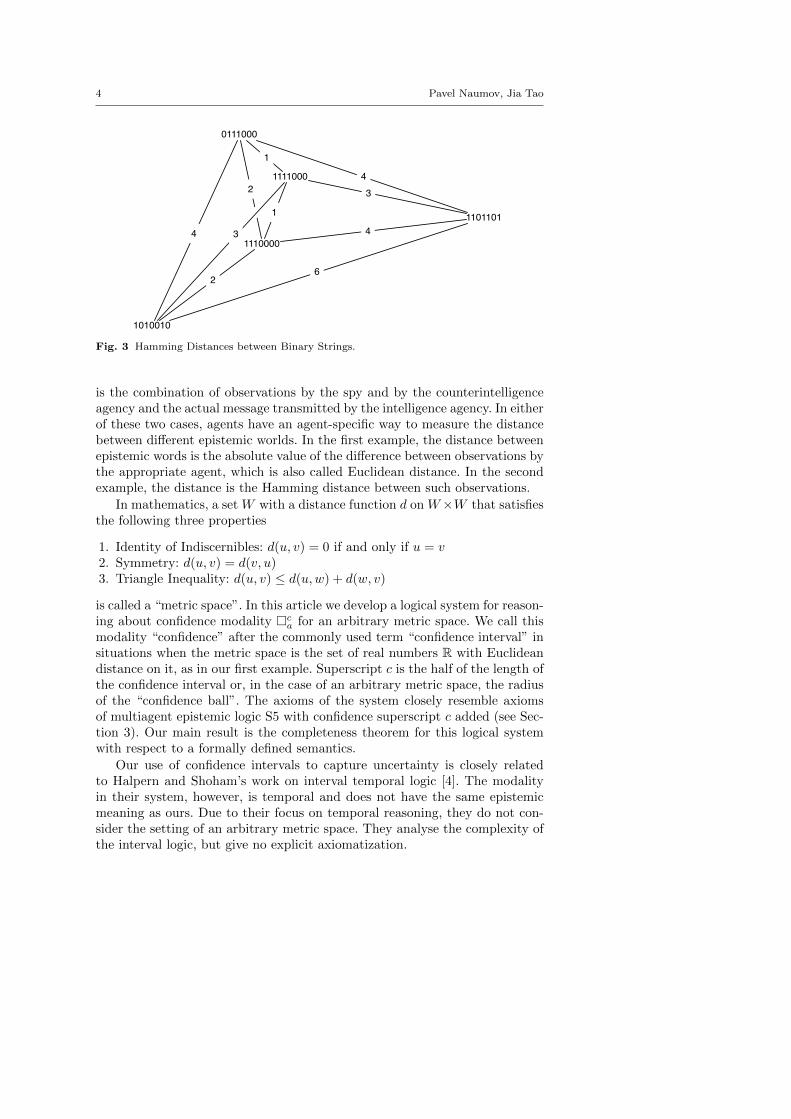
An easy way (see Figure 3) to visualize this situation is to draw a pictureshowing each binary string as a point. For any two strings, the “distance”between them is the number of positions at which digits of these two stringsdiffer. This distance is known as Hamming distance [5].

In our first example, the data about a vehicle shown in Figure 1, togetherwith its actual speed, could be thought of as an “epistemic world” in thetraditional epistemic logic sense. In the second example, the epistemic world


1010010

0111000

41101101

6

4

1110000

2

2

4

1111000

1

1

3

3

Fig. 3 Hamming Distances between Binary Strings.

is the combination of observations by the spy and by the counterintelligenceagency and the actual message transmitted by the intelligence agency. In eitherof these two cases, agents have an agent-specific way to measure the distancebetween different epistemic worlds. In the first example, the distance betweenepistemic words is the absolute value of the difference between observations bythe appropriate agent, which is also called Euclidean distance. In the secondexample, the distance is the Hamming distance between such observations.

In mathematics, a set W with a distance function d on W×W that satisfiesthe following three properties

1. Identity of Indiscernibles: d(u, v) = 0 if and only if u = v2. Symmetry: d(u, v) = d(v, u)3. Triangle Inequality: d(u, v) ≤ d(u,w) + d(w, v)

is called a “metric space”. In this article we develop a logical system for reason-ing about confidence modality �c

a for an arbitrary metric space. We call thismodality “confidence” after the commonly used term “confidence interval” insituations when the metric space is the set of real numbers R with Euclideandistance on it, as in our first example. Superscript c is the half of the length ofthe confidence interval or, in the case of an arbitrary metric space, the radiusof the “confidence ball”. The axioms of the system closely resemble axiomsof multiagent epistemic logic S5 with confidence superscript c added (see Sec-tion 3). Our main result is the completeness theorem for this logical systemwith respect to a formally defined semantics.

Our use of confidence intervals to capture uncertainty is closely relatedto Halpern and Shoham’s work on interval temporal logic [4]. The modalityin their system, however, is temporal and does not have the same epistemicmeaning as ours. Due to their focus on temporal reasoning, they do not con-sider the setting of an arbitrary metric space. They analyse the complexity ofthe interval logic, but give no explicit axiomatization.


Milnikel [8] proposed a version of justification logic [1] with uncertain justi-fications. His system studies the degrees up to which an agent is confident thatcertain evidence justifies the formula. The difference between our and his ap-proaches manifests itself most explicitly in the modal distributivity axiom. Inour system (see Section 3) the distributivity axiom is: �c

a(ϕ→ ψ)→ (�caϕ→

�caψ). Informally, it states that if agent a is confident in ϕ → ψ, assuming

precision of measurements ±c, and she is also confident in ϕ, assuming thesame precision of measurements, then she is confident in ψ, again with thesame precision. The corresponding axiom in Milnikel’s system [8] could bewritten as �c

a(ϕ → ψ) → (�dbϕ → �c·d

a,bψ), where c · d is the product of tworeal numbers representing agent’s degrees of confidence that the combinationof justifications a and b supports claim ψ.

Our work at its core is very much connected to Moss and Parikh’s work ontopological reasoning and epistemic logic [9]. Similar to ours, their work startedwith confidence intervals, although they did not use this term explicitly. Thesame example about the accuracy of a police officer’s knowledge of the speedof a car was used to introduce the topic. They chose, however, a much moregeneral setting than ours. Instead of generalizing from confidence intervalson a number line to a “ball” in an arbitrary metric space as we do, theywent one step further by interpreting it as an open set in a topological space.The smaller such a set is the more precise the knowledge is. As a result, theirlogical system can reason about different levels of precision without assigning anumerical value to this precision. They also separated the knowledge modalityinto two different modal operators: one representing the knowledge and theother representing the precision of the knowledge (or, to use their terminology,“the effort”).

Finally, our work could also be thought of as a study of spatial reasoningin an arbitrary metric space. The satisfiability relation w �c

aϕ, from such aperspective, could be interpreted as “statement ϕ is true in c-neghbourhoodof point w under the metric associated with agent a”. This relates our systemto other modal logics for spatial reasoning [12,3].

The rest of the article is structured as follows. Section 2 formally specifiessyntax and semantics of the logical system. Section 3 introduces its axiomsand inference rules. The soundness of the system with respect to the formalsemantics is shown in Section 4. The proof of the completeness is divided intotwo parts. Section 5 considers metric spaces in which distances between pointscould be infinite and proves the completeness theorem with respect to theclass of confidence models based on such metric spaces. The proof employsthe “unravelling” [11] technique from modal logic model theory. Section 6uses truncation of metric spaces to prove the completeness for the class ofconfidence models based on the metric spaces with finite distances. Section 7discusses possible generalizations of our logic to group confidence as well asits connections to standard Kripke models and judgement aggregation.


2 Syntax and Semantics

In this section we formally define syntax and semantics of our logical system.We assume a fixed set P of atomic propositions and a fixed set A of agents.

Definition 1 Let Φ be the smallest set of formulas such that

1. P ⊆ Φ,2. if ϕ,ψ ∈ Φ, then ¬ϕ ∈ Φ and ϕ→ ψ ∈ Φ,3. if ϕ ∈ Φ, then �c

aϕ ∈ Φ, for each a ∈ A, and each real number c ≥ 0.

Below is the standard definition of a metric space [10]. Hamming dis-tance [5], Manhattan distance [7], shortest path distance, and Euclidean spacedistance are standard examples of such metric spaces.

Definition 2 A finite metric space is a pair (W,d) such that W is a set and dis a distance function between two elements of W whose value is a non-negativereal number. Additionally, function d must satisfy the following properties forall u, v, w ∈W :

1. Identity of Indiscernibles: d(u, v) = 0 if and only if u = v,2. Symmetry: d(u, v) = d(v, u),3. Triangle Inequality: d(u, v) ≤ d(u,w) + d(w, v).

In the above definition, as in some of the literature on metric spaces [2], weuse the term finite metric space. In Section 5, we consider a more generaldefinition of a metric space in which distances can be infinite.

Definition 3 A finite confidence model is a tuple (W, {da}a∈A, π), such that(W,da) is a finite metric space for each a ∈ A and π is a function fromatomic propositions into subsets of W . Elements of set W are called “epistemicworlds”.

In Section 7, we discuss relation between finite confidence models and standardKripke models used in epistemic logic.

Definition 4 For any world w of a finite confidence model (W, {da}a∈A, π)and any formula ϕ ∈ Φ, we define satisfiability relation w ϕ as follows:

1. w p if w ∈ π(p), where p ∈ P,2. w ¬ψ if w 1 ψ, where ψ ∈ Φ,3. w ψ1 → ψ2 if w 1 ψ1 or w ψ2, where ψ1, ψ2 ∈ Φ,4. w �c

aψ if u ψ for each epistemic world u ∈W such that da(w, u) ≤ c,where ψ ∈ Φ, a ∈ A, and c ≥ 0.

3 Axioms and Inference Rules

Our logical system, in addition to propositional tautologies in language Φ,contains the following axioms:


1. Zero Confidence: ϕ→ �0aϕ,

2. Truth: �caϕ→ ϕ,

3. Positive Introspection: �c+da ϕ→ �c

a�daϕ,

4. Negative Introspection: ¬�caϕ→ �d

a¬�c+da ϕ,

5. Distributivity: �ca(ϕ→ ψ)→ (�c

aϕ→ �caψ).

We write ` ϕ if formula ϕ is provable from the propositional tautologies andthe above axioms using Modus Ponens and Necessitation inference rules:

ϕ, ϕ→ ψ

ψ

ϕ

�caϕ

We write X ` ϕ if formula ϕ is provable from propositional tautologies, theabove axioms, and the additional set of axioms X using only Modus Ponensinference rule.

4 Soundness

In this section we establish the soundness of our logical system with respect tothe semantics given in Definition 2. The soundness of propositional tautologiesand of Modus Ponens inference rule is straightforward. Below we prove thesoundness of each remaining axiom and of the Necessitation inference rule asa separate lemma. We assume that w is an arbitrary epistemic world of a finiteconfidence model (W, {da}a∈A, π).

Lemma 1 (Zero Confidence) For any formula ϕ ∈ Φ and any a ∈ A, ifw ϕ, then w �0

aϕ.

Proof We need to prove that u ϕ for each u ∈W such that da(w, u) = 0. ByIdentity of Indiscernibles property of metric spaces (see Definition 2), equalityda(w, u) = 0 implies w = u. Hence, u ϕ due to the assumption w ϕ. ut

Lemma 2 (Truth) For any formula ϕ ∈ Φ, any a ∈ A, and any real numberc ≥ 0, if w �c

aϕ, then w ϕ.

Proof Suppose that w �caϕ. By Identity of Indiscernibles property of met-

ric spaces (see Definition 2), da(w,w) = 0. Thus, da(w,w) ≤ c. Hence, byDefinition 4, w ϕ. ut

Lemma 3 (Positive Introspection) For any formula ϕ ∈ Φ, any a ∈ A,and any real numbers c, d ≥ 0, if w �c+d

a ϕ, then w �ca�

daϕ.

Proof Consider any u ∈ W such that da(w, u) ≤ c. By Definition 4, it suf-fices to show that u �d

aϕ. Indeed, let v ∈ W be any epistemic world suchthat da(u, v) ≤ d. We need to prove that v ϕ. By Triangle Inequality,da(w, v) ≤ da(w, u) + da(u, v) ≤ c + d. Thus, due to assumption w �c+d

a ϕand Definition 4, v ϕ. ut


Lemma 4 (Negative Introspection) For any formula ϕ ∈ Φ, any a ∈ A,and any real numbers c, d ≥ 0, if w ¬�c

aϕ, then w �da¬�c+d

a ϕ.

Proof By Definition 4, assumption w ¬�caϕ implies the existence of an

epistemic world u ∈ W such that da(w, u) ≤ c and u 1 ϕ. To prove w �d

a¬�c+da ϕ, consider any v ∈W such that da(w, v) ≤ d. It suffices to show that

v 1 �c+da ϕ. Indeed, by Triangle Inequality, da(v, u) ≤ da(v, w)+da(w, u) ≤ d+

c. Additionally, u 1 ϕ due to the choice of world u. Therefore, by Definition 4,v 1 �c+d

a ϕ. ut

Lemma 5 (Distributivity) For any formulas ϕ,ψ ∈ Φ, any a ∈ A, and anyreal number c ≥ 0, if w �c

a(ϕ→ ψ) and w �caϕ, then w �c

aψ.

Proof Consider any u ∈ W such that da(w, u) ≤ c. It suffices to show thatu ψ. Indeed, u ϕ → ψ and u ϕ due to Definition 4 and assumptionsw �c

a(ϕ → ψ) and w �caϕ respectively. Therefore, again by Definition 4,

u ψ. ut

Lemma 6 (Necessitation) For any formula ϕ ∈ Φ, if u ϕ for each worldu of each finite confidence model, then u �c

aϕ for each world u of each finiteconfidence model, where a ∈ A and c is a non-negative real number.

Proof Suppose that v ∈W is such that da(u, v). It suffices to show that v ϕ,which is true due to the assumption of the lemma. ut

5 Completeness for Confidence Models

The goal of this and the next section is to prove the completeness theoremfor our logical system with respect to finite confidence models specified inDefinition 3. This result is obtained in two steps. In this section, we generalizefinite confidence models to confidence models and prove the completeness ofour system with respect to this class of more general models. The proof employsthe “unravelling” [11] technique from modal logic model theory. In the nextsection, we show how to convert a confidence model to a finite confidencemodel, using a technique from metric space theory sometimes (for example,in [6]) called “truncation”.

5.1 Metric Space and Confidence Models

In Definition 2, we require each distance to be a finite real number. It issometimes more convenient to use a more general notion of a metric spacewith possibly infinite distances. Following [2], we refer to the more generalnotion as just a metric space as opposed to the earlier discussed notion of afinite metric space.


Definition 5 A metric space is a pair (W,d) such that W is a set and d is adistance function between two elements ofW whose value is a non-negative realnumber or ∞. Additionally, function d must satisfy the following propertiesfor all u, v, w ∈W :

1. Identity of Indiscernibles: d(u, v) = 0 if and only if u = v,2. Symmetry: d(u, v) = d(v, u),3. Triangle Inequality: d(u, v) ≤ d(u,w) + d(w, v).

In the above definition we assume that ∞ +∞ = ∞ and ∞ + r = ∞, wherer is any non-negative real number.

We define a more general notion of a confidence model using metric spacesin the same way finite confidence models are specified in Definition 3 usingfinite metric spaces.

Definition 6 A confidence model is a tuple (W, {da}a∈A, π), such that (W,da)is a metric space for each a ∈ A and π is a function from atomic propositionsinto subsets of W . Elements of set W are called “epistemic worlds”.

The satisfiability relation for confidence models is defined below in thesame way as in the case of finite confidence models (Definition 4).

Definition 7 For any world w of an confidence model (W, {da}a∈A, π) andany formula ϕ ∈ Φ, we define satisfiability relation w ϕ as follows:

1. w p if w ∈ π(p), where p ∈ P,2. w ¬ψ if w 1 ψ, where ψ ∈ Φ,3. w ψ1 → ψ2 if w 1 ψ1 or w ψ2, where ψ1, ψ2 ∈ Φ,4. w �c

aψ if u ψ for each epistemic world u ∈W such that da(w, u) ≤ c,where ψ ∈ Φ, a ∈ A, and c ≥ 0.

5.2 Canonical Confidence Model

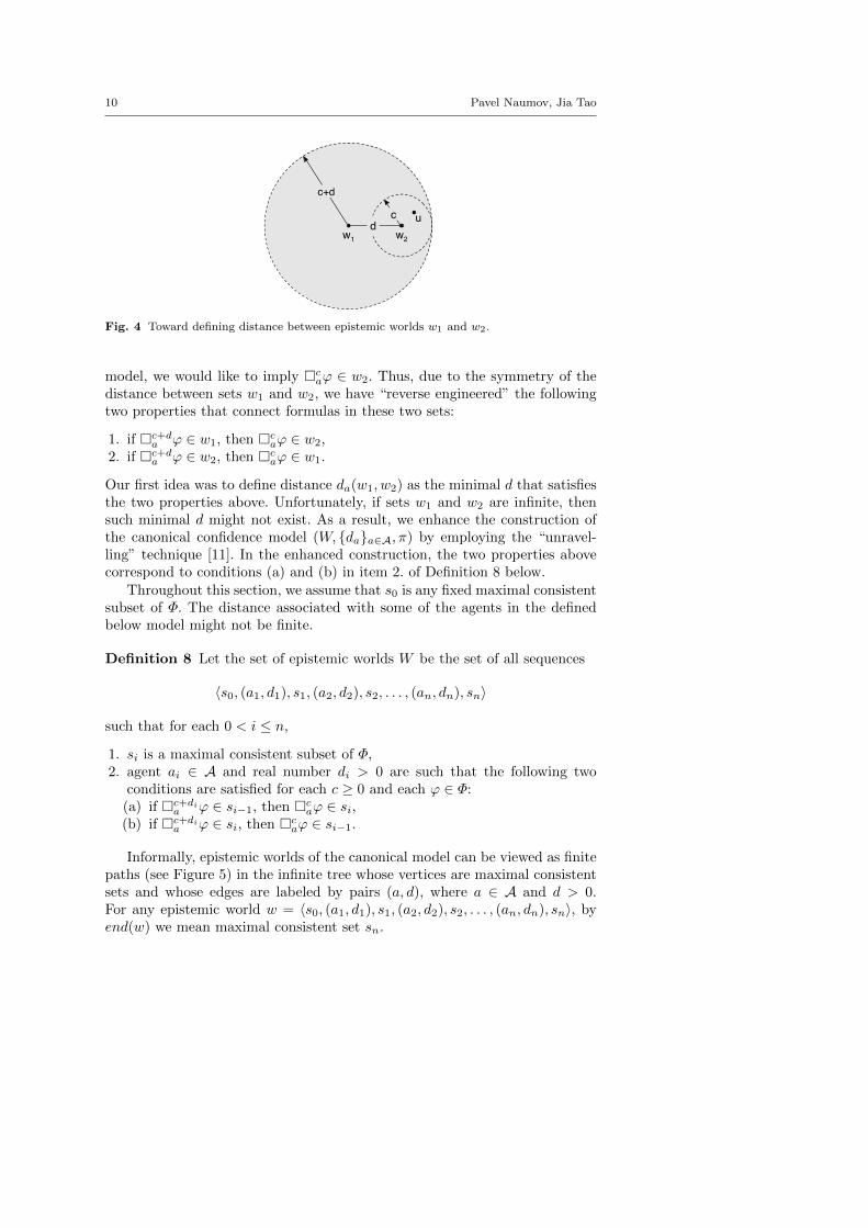
In this section we modify the standard canonical epistemic model constructionto produce a canonical confidence model. The epistemic worlds in the canonicalepistemic model are usually defined as maximal consistent sets of formulas.Two such sets w1 and w2 are indistinguishable to an agent a when �aϕ ∈ w1 ifand only if �aϕ ∈ w2 for each formula ϕ. To construct a canonical confidencemodel, instead of indistinguishability relation, we need to define the distancebetween maximal consistent sets w1 and w2 under the metric associated withany given agent a. We “reverse engineer” this definition by assuming that thedistance between w1 and w2 is d (see Figure 4) and by studying the relationbetween formulas in sets w1 and w2.

Suppose that �c+da ϕ ∈ w1. We would like this to imply that in our canonical

model w1 �c+da ϕ. Then, by Definition 7, u ϕ for each world u inside

the ball of radius c + d around epistemic world w1. Hence, by the TriangleInequality, u ϕ for each u inside the ball of radius c around epistemicworld w2 (see Figure 4). In other words, w2 �c

aϕ, which, in our canonical


c+d

cd

w1 w2

u

Fig. 4 Toward defining distance between epistemic worlds w1 and w2.

model, we would like to imply �caϕ ∈ w2. Thus, due to the symmetry of the

distance between sets w1 and w2, we have “reverse engineered” the followingtwo properties that connect formulas in these two sets:

1. if �c+da ϕ ∈ w1, then �c

aϕ ∈ w2,2. if �c+d

a ϕ ∈ w2, then �caϕ ∈ w1.

Our first idea was to define distance da(w1, w2) as the minimal d that satisfiesthe two properties above. Unfortunately, if sets w1 and w2 are infinite, thensuch minimal d might not exist. As a result, we enhance the construction ofthe canonical confidence model (W, {da}a∈A, π) by employing the “unravel-ling” technique [11]. In the enhanced construction, the two properties abovecorrespond to conditions (a) and (b) in item 2. of Definition 8 below.

Throughout this section, we assume that s0 is any fixed maximal consistentsubset of Φ. The distance associated with some of the agents in the definedbelow model might not be finite.

Definition 8 Let the set of epistemic worlds W be the set of all sequences

〈s0, (a1, d1), s1, (a2, d2), s2, . . . , (an, dn), sn〉

such that for each 0 < i ≤ n,

1. si is a maximal consistent subset of Φ,2. agent ai ∈ A and real number di > 0 are such that the following two

conditions are satisfied for each c ≥ 0 and each ϕ ∈ Φ:(a) if �c+di

a ϕ ∈ si−1, then �caϕ ∈ si,

(b) if �c+dia ϕ ∈ si, then �c

aϕ ∈ si−1.

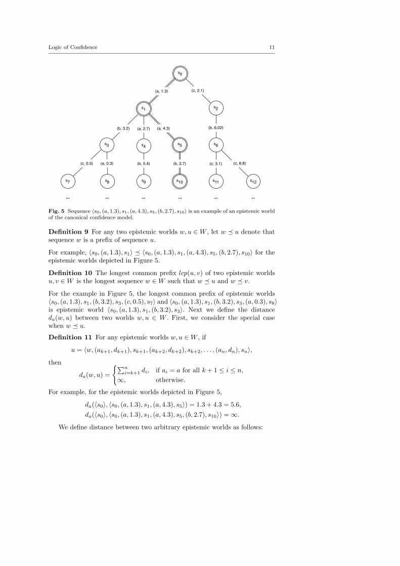
Informally, epistemic worlds of the canonical model can be viewed as finitepaths (see Figure 5) in the infinite tree whose vertices are maximal consistentsets and whose edges are labeled by pairs (a, d), where a ∈ A and d > 0.For any epistemic world w = 〈s0, (a1, d1), s1, (a2, d2), s2, . . . , (an, dn), sn〉, byend(w) we mean maximal consistent set sn.


s2s1

s0

s3 s4 s5 s6

s11 s12s9 s10s8s7

(a, 1.3) (c, 2.1)

(b, 3.2)

(c, 0.5) (a, 0.3)

(a, 4.3)(a, 2.7)

(b, 5.4) (b, 2.7)

(b, 6.02)

(c, 8.8)(c, 3.1)

... ... ... ... ... ...

Fig. 5 Sequence 〈s0, (a, 1.3), s1, (a, 4.3), s5, (b, 2.7), s10〉 is an example of an epistemic worldof the canonical confidence model.

Definition 9 For any two epistemic worlds w, u ∈ W , let w � u denote thatsequence w is a prefix of sequence u.

For example, 〈s0, (a, 1.3), s1〉 � 〈s0, (a, 1.3), s1, (a, 4.3), s5, (b, 2.7), s10〉 for theepistemic worlds depicted in Figure 5.

Definition 10 The longest common prefix lcp(u, v) of two epistemic worldsu, v ∈W is the longest sequence w ∈W such that w � u and w � v.

For the example in Figure 5, the longest common prefix of epistemic worlds〈s0, (a, 1.3), s1, (b, 3.2), s3, (c, 0.5), s7〉 and 〈s0, (a, 1.3), s1, (b, 3.2), s3, (a, 0.3), s8〉is epistemic world 〈s0, (a, 1.3), s1, (b, 3.2), s3〉. Next we define the distanceda(w, u) between two worlds w, u ∈ W . First, we consider the special casewhen w � u.

Definition 11 For any epistemic worlds w, u ∈W , if

u = 〈w, (ak+1, dk+1), sk+1, (ak+2, dk+2), sk+2, . . . , (an, dn), sn〉,

then

da(w, u) =

{∑ni=k+1 di, if ai = a for all k + 1 ≤ i ≤ n,

∞, otherwise.

For example, for the epistemic worlds depicted in Figure 5,

da(〈s0〉, 〈s0, (a, 1.3), s1, (a, 4.3), s5〉) = 1.3 + 4.3 = 5.6,

da(〈s0〉, 〈s0, (a, 1.3), s1, (a, 4.3), s5, (b, 2.7), s10〉) =∞.

We define distance between two arbitrary epistemic worlds as follows:


Definition 12 For any two epistemic worlds u, v ∈ W , the distance betweenu and v is: da(u, v) = da(lcp(u, v), u) + da(lcp(u, v), v).

For example, for the epistemic worlds depicted in Figure 5,

da(〈s0, (a, 1.3), s1, (a, 2.7), s4〉, 〈s0, (a, 1.3), s1, (a, 4.3), s5〉) = 2.7 + 4.3 = 7.0,

da(〈s0, (a, 1.3), s1, (b, 3.2), s3〉, 〈s0, (a, 1.3), s1, (a, 4.3), s5〉) =∞.

Lemma 7 For any two worlds w, u ∈W such that w � u and da(w, u) ≤ c,

1. if �caϕ ∈ end(w), then �c−da(w,u)

a ϕ ∈ end(u),

2. if �caϕ ∈ end(u), then �c−da(w,u)

a ϕ ∈ end(w).

Proof We prove by induction on the length of sequence u.Base Case: w = u. Then the required follows from da(w, u) = 0.Induction Step: The induction step for parts 1 and 2 of the lemma follows,respectively, from conditions a) and b) of part 2 of Definition 8. ut

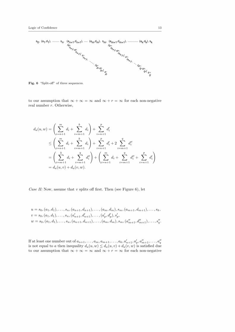
Shortest path distance between any two points of an arbitrary weightedgraph satisfies all conditions in Definition 2 and, thus, specifies metric betweenvertices of the graph. By definition, a tree is a graph that has exactly one pathwithout self-intersections between any two vertices. Thus, the length of sucha path is a metric on vertices of an arbitrary weighted tree. One can see thatfunction da(w, u) is equal to the length of the shortest path between verticesend(w) and end(v) on the tree partially depicted in Figure 5. This impliesthat da is a metric on the set of epistemic worlds W . However, since we havenever formally defined the class of trees whose example is depicted in Figure 5,our proof below, instead of using shortest distance argument, directly refersto Definition 12.

Lemma 8 The pair (W,da) is a metric space for each a ∈ A.

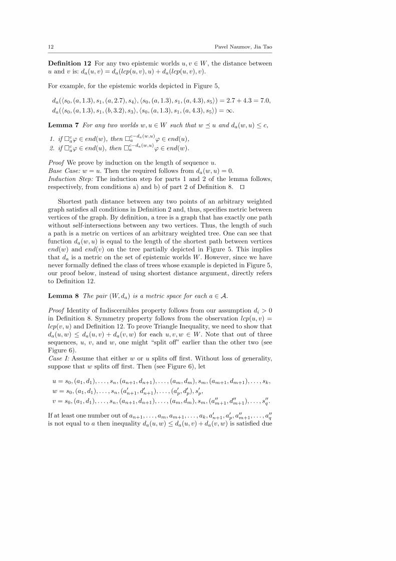
Proof Identity of Indiscernibles property follows from our assumption di > 0in Definition 8. Symmetry property follows from the observation lcp(u, v) =lcp(v, u) and Definition 12. To prove Triangle Inequality, we need to show thatda(u,w) ≤ da(u, v) + da(v, w) for each u, v, w ∈ W . Note that out of threesequences, u, v, and w, one might “split off” earlier than the other two (seeFigure 6).Case I: Assume that either w or u splits off first. Without loss of generality,suppose that w splits off first. Then (see Figure 6), let

u = s0, (a1, d1), . . . , sn, (an+1, dn+1), . . . , (am, dm), sm, (am+1, dm+1), . . . , sk,

w = s0, (a1, d1), . . . , sn, (a′n+1, d

′n+1), . . . , (a′p, d

′p), s′p,

v = s0, (a1, d1), . . . , sn, (an+1, dn+1), . . . , (am, dm), sm, (a′′m+1, d

′′m+1), . . . , s′′q .

If at least one number out of an+1, . . . , am, am+1, . . . , ak, a′n+1, a

′p, a′′m+1, . . . , a

′′q

is not equal to a then inequality da(u,w) ≤ da(u, v) + da(v, w) is satisfied due


sn,s0, (ak,dk), sk

(a'p ,d'p ), s'p

(a'n+1 ,d'n+1 ), s'n+1 ,

(a1,d1), (an+1,dn+1), (am,dm), sm,(a''m+1 ,d''m+1 ), s''m+1 ,

(a''q ,d''q ), s''q

(am+1,dm+1),

Fig. 6 “Split-off” of three sequences.

to our assumption that ∞ +∞ = ∞ and ∞ + r = ∞ for each non-negativereal number r. Otherwise,

da(u,w) =

(m∑

i=n+1

di +k∑

i=m+1

di

)+

p∑i=n+1

d′i

≤

(m∑

i=n+1

di +

k∑i=m+1

di

)+

p∑i=n+1

d′i + 2

q∑i=m+1

d′′i

=

(k∑

i=m+1

di +

q∑i=m+1

d′′i

)+

(m∑

i=n+1

di +

q∑i=m+1

d′′i +

p∑i=n+1

d′i

)= da(u, v) + da(v, w).

Case II: Now, assume that v splits off first. Then (see Figure 6), let

u = s0, (a1, d1), . . . , sn, (an+1, dn+1), . . . , (am, dm), sm, (am+1, dm+1), . . . , sk,

v = s0, (a1, d1), . . . , sn, (a′n+1, d

′n+1), . . . , (a′p, d

′p), s′p,

w = s0, (a1, d1), . . . , sn, (an+1, dn+1), . . . , (am, dm), sm, (a′′m+1, d

′′m+1), . . . , s′′q .

If at least one number out of an+1, . . . , am, am+1, . . . , ak, a′n+1, a

′p, a′′m+1, . . . , a

′′q

is not equal to a then inequality da(u,w) ≤ da(u, v) + da(v, w) is satisfied dueto our assumption that ∞ +∞ = ∞ and ∞ + r = ∞ for each non-negative


real number r. Otherwise, by Definition 12,

da(u,w) =

k∑i=m+1

di +

q∑i=m+1

d′′i

=

k∑i=m+1

di +

q∑i=m+1

d′′i + 2

p∑i=n+1

d′i + 2

m∑i=n+1

di

=

(m∑

i=n+1

di +

k∑i=m+1

di +

p∑i=n+1

d′i

)

+

(p∑

i=n+1

d′i +

m∑i=n+1

di +

q∑i=m+1

d′′i

)= da(u, v) + da(v, w).

ut

Definition 13 π(p) = {w ∈W | p ∈ end(w)} for any atomic proposition p.

This concludes the definition of the canonical confidence model (W, {da}a∈A, π).Remaining lemmas in this section describe various properties of the canonicalmodel needed for the proof of completeness.

Lemma 9 For any two worlds u, v ∈ W , if �caϕ ∈ end(u) and da(u, v) ≤ c,

then ϕ ∈ end(v).

Proof Consider w = lcp(u, v). By Part 2 of Lemma 7, assumption �caϕ ∈

end(u) implies that �c−d(u,w)a ϕ ∈ end(w). Note that da(u,w) + da(w, v) =

da(u, v) ≤ c by Definition 12. Hence, by Part 1 of Lemma 7,

�c−da(u,w)−da(w,v)a ϕ ∈ end(v).

Thus, �c−da(u,v)a ϕ ∈ end(v) by again Definition 12. Thus, end(v) ` ϕ by Truth

axiom. Therefore, ϕ ∈ end(v) due to the maximality of the set end(v). ut

Lemma 10 For any epistemic world w ∈ W , if �caϕ /∈ end(w), then there is

a world u ∈W such that ϕ /∈ end(u) and da(w, u) = c.

Proof If c = 0, then choose u to be world w. Suppose that ϕ ∈ end(w). Thus,end(w) ` �0

aϕ by Zero Confidence axiom. Hence, �0aϕ ∈ end(w) due to the

maximality of set w, which contradicts the assumption of the lemma.Suppose that c > 0. We first show that the following set is consistent

X = {¬ϕ} ∪ {�daψ | �d+c

a ψ ∈ end(w)} ∪ {¬�d+ca χ | ¬�d

aχ ∈ end(w)}.

Assume the opposite. Thus, there must exist

�d1+ca ψ1, . . . ,�

dn+ca ψn,¬�

d′1

a χ1, . . . ,¬�d′m

a χm ∈ end(w) (1)


such that

�d1a ψ1, . . . ,�

dna ψn,¬�

d′1+c

a χ1, . . . ,¬�d′m+c

a χm ` ϕ.

Hence, by Deduction theorem for propositional logic,

` �d1a ψ1 → (. . . (�dn

a ψn → (¬�d′1+c

a χ1 → (. . . (¬�d′m+c

a χm → ϕ) . . . ))) . . . ).

Thus, by Necessitation rule,

` �ca(�d1

a ψ1 → (. . . (�dna ψn → (¬�d′

1+ca χ1 → (. . . (¬�d′

m+ca χm → ϕ) . . . ))) . . . )).

By Distributivity axiom and Modus Ponens rule,

�ca�

d1a ψ1 ` �c

a(�d2a ψ2 → (· · · → (¬�d′

m+ca χm → ϕ) . . . )).

By repeating the previous step (n+m− 1) times,

�ca�

d1a ψ1, . . . ,�

ca�

dna ψn,�

ca¬�

d′1+c

a χ1, . . . ,�ca¬�

d′m+c

a χm ` �caϕ.

By Positive Introspection axiom applied n times,

�d1+ca ψ1, . . . ,�

dn+ca ψn,�

ca¬�

d′1+c

a χ1, . . . ,�ca¬�

d′m+c

a χm ` �caϕ.

By Negative Introspection axiom applied m times,

�d1+ca ψ1, . . . ,�

dn+ca ψn,¬�

d′1

a χ1, . . . ,¬�d′m

a χm ` �caϕ.

Hence, end(w) ` �caϕ, due to assumption (1). Thus, due to the maximality

of end(w), we have �caϕ ∈ end(w), which contradicts the assumption of the

lemma. Therefore, setX is consistent. Let X be a maximal consistent extensionof X. Define u to be the extension of sequence w such that u = w, (a, c), X. ByDefinition 8 and due to the assumption c > 0, we have u ∈W . By Definition 11,d(w, u) = c. ut

Lemma 11 w ϕ if and only if ϕ ∈ end(w), for any epistemic world w ∈Wand any formula ϕ ∈ Φ.

Proof We prove the lemma by induction on the structural complexity of for-mula ϕ. If ϕ is an atomic proposition, then the required follows from Defini-tion 13 and Definition 7. If formula ϕ is of the form ¬ψ or ψ → χ, then therequired follows from maximality and consistency of the set end(w), Defini-tion 7 and the induction hypothesis in the standard way. Suppose that ϕ is ofthe form �c

aψ.(⇒) : If �c

aψ /∈ end(w), then, by Lemma 10, there exists u ∈ W such thatda(w, u) = c and ψ /∈ end(u). Thus, by the induction hypothesis, u 1 ψ.Therefore, by Definition 7, w 1 �c

aψ.(⇐) : Assume that w 1 �c

aψ. Hence, by Definition 7, there must exist u ∈Wsuch that u 1 ψ and da(w, u) ≤ c. Thus, by the induction hypothesis, ψ /∈end(u). Therefore, by Lemma 9, �c

aψ /∈ end(w). ut


5.3 Completeness Theorem

We are now ready to state and prove the completeness theorem for (not nec-essarily finite) confidence models.

Theorem 1 If w ϕ for each epistemic world w of each confidence model,then ` ϕ.

Proof Suppose that 0 ϕ. Let s0 be any maximal consistent set containing ¬ϕ.Consider the canonical model defined, based on s0, in Section 5.2. Note thatsingle-element sequence s0 is a world of the canonical model. By Lemma 11,s0 1 ϕ. ut

6 Completeness for Finite Confidence Models

In this section we use the truncation operation on metric spaces to strengthenour completeness theorem from the class of all confidence models to the classof finite confidence models.

6.1 Truncation of Metric Spaces

Definition 14 For any metric space (W,d), any u, v ∈ W , and any positive(“threshold”) real number t, let truncated distance d�t be defined as

d�t(u, v) =

{d(u, v), if d(u, v) ≤ t,t, otherwise.

Lemma 12 (X, d�t) is a finite metric space for each metric space (X, d) andeach positive real threshold value t.

Proof Identity of Indiscernibles and Symmetry properties follow from Defini-tion 14 and Definition 5. To prove Triangle Inequality, for any world w ∈ Wwe prove that d�t(u, v) ≤ d�t(u,w) + d�t(w, v). If max{d(u,w), d(w, v)} ≥ t,then max{d�t(u,w), d�t(w, v)} = t. Thus,

d�t(u, v) ≤ t = max{d�t(u,w), d�t(w, v)} ≤ d�t(u,w) + d�t(w, v).

Otherwise, max{d(u,w), d(w, v)} < t. Thus, d�t(u,w) + d�t(w, v) = d(u,w) +d(w, v). Hence, by Triangle Inequality for metric d,

d�t(u, v) ≤ d(u, v) ≤ d(u,w) + d(w, v) = d�t(u,w) + d�t(w, v).

ut


6.2 Truncation of Confidence Models

Definition 15 For any confidence model (W, {da}a∈A, π) and any real num-ber t, let truncation of this model with threshold value t be triple (W, {da�t}a∈A, π).

The following lemma follows from Definition 15 and Lemma 12.

Lemma 13 For any any confidence model (W, {da}a∈A, π) and any thresholdvalue t > 0, truncation (W, {da�t}a∈A, π) is a finite confidence model.

Informally, rank(ϕ) is the largest modality superscript c that appears in-side formula ϕ. Formally, rank(ϕ) is defined below.

Definition 16 For any formula ϕ ∈ Φ, the non-negative value rank(ϕ) isdefined recursively as follows:

1. rank(p) = 0 for each atomic proposition p,2. rank(¬ψ) = rank(ψ), for each ψ ∈ Φ,3. rank(ψ → χ) = max{rank(ψ), rank(χ)}, for each ψ, χ ∈ Φ,4. rank(�c

aψ) = max{c, rank(ψ)}, for each c ≥ 0, a ∈ A, ψ ∈ Φ.

Lemma 14 If is satisfiability relation of a confidence model (W, {da}a∈A, π)and ′ is satisfiablility relation of model (W, {da�t}a∈A, π), then w ϕ if andonly if w ′ ϕ, for any ϕ ∈ Φ such that rank(ϕ) ≤ t.

Proof We prove by induction on structural complexity of formula ϕ. If ϕ is anatomic proposition p, then, by Definition 4, both w p and w ′ p are equiv-alent to statement w ∈ π(p). Thus, w p if and only if w ′ p. Cases when ϕis a negation or an implication follow from the induction hypothesis, Defini-tion 4, and Definition 7. Assume now that ϕ is �c

aψ. Then, by Definition 16,c ≤ t and rank(ψ) ≤ t.(⇒) : Suppose that w 1′ �c

aψ. Thus, by Definition 4, there is u ∈W such thatda�t(w, u) ≤ c and u 1′ ψ. Then, da(w, u) ≤ c due to c ≤ t and Definition 14.Also, by the induction hypothesis, u 1 ψ. Therefore, w 1 �c

aψ by Definition 7.(⇐) : Assume that w 1 �c

aψ. Thus, by Definition 7, there is u ∈ W suchthat da(w, u) ≤ c and u 1 ψ. Then, da�t(w, u) ≤ da(w, u) ≤ c. Also, by theinduction hypothesis, u 1′ ψ. Therefore, w 1′ �c

aψ by Definition 4. ut

6.3 Completeness Theorem

We now state and prove the main completeness result of this article.

Theorem 2 If w ϕ for each epistemic world w of each finite confidencemodel, then ` ϕ.

Proof Suppose that 0 ϕ. By Theorem 1, there is an epistemic world w of aconfidence model (W, {da}a∈A, π) such that w 1 ϕ. Let ′ be satisfiability re-lation for truncated confidence model (W, {da�rank(ϕ)}a∈A, π). By Lemma 14,w 1′ ϕ. ut


7 Discussion

In this article we studied epistemic modality expressing confidence of a singleagent in a multiagent system. Similar to the notion of distributed knowledgemodality in epistemic logic, one may consider using formula �c

Aϕ, where Ais an arbitrary set of agents, to express “group confidence” in statement ϕ.There are, however, at least two different ways to interpret this modality. Onecan say that formula �c

Aϕ is satisfied in epistemic world w if formula ϕ issatisfied in each epistemic world that is no further than c away from w in themetric of each agent a ∈ A. Alternatively, one can require the total sum of alldistances for all a ∈ A to be no more than c. These two definitions of groupconfidence have different modal properties. For example, the first definition

satisfies property �cAϕ → (�d

Bϕ → �max{c,d}A∪B ϕ). The second definition yields

a stronger form of this property: �cAϕ→ (�d

Bϕ→ �c+dA∪Bϕ).

One can also define “common confidence” modality CcAϕ among a group

of agents A. Namely, w CcAϕ is true if for any sequence of epistemic worlds

w0, . . . , wn and any a1, . . . , an ∈ A if w = w0 and∑

1≤i≤n dai(wi−1, wi) < c,

then wn ϕ.

If Identity of Indiscernibles in Definition 5 is replaced with a weaker con-dition: d(u, u) = 0, then the resulting mathematical structure is known aspseudo metric space. Accordingly, if da in Definition 6 is assumed to be onlya pseudo metric, then we call the resulting structure pseudo confidence model.Of a particular interest are pseudo confidence models in which any distance iseither 0 or ∞. All epistemic worlds in such models are partitioned into classessuch that distance between worlds in the same class is zero. Thus, any suchmodel is isomorphic to a standard S5 Kripke model, where confidence modality�0

a is translated to epistemic modality �a.

There is a connection between confidence reasoning and judgement aggre-gation. Indeed, consider an epistemic world w ∈ W of an S5 Kripke model(W, {∼a}a∈A, π), where A is a set of agents. One can introduce judgementaggregation modality �nϕ to represent the fact that at most n agents in setA do not know that ϕ is true:

w �nϕ if there is A0 ⊆ A such that (i) |A \ A0| ≤ n and (ii) for anya ∈ A0, if w ∼a v, then v ϕ.

Alternatively, one can define judgement aggregation modality �nϕ to representthe fact that ϕ is true in all epistemic worlds indistinguishable from the currentworld by all except for at most n agents in set A:

w �nϕ if v ϕ for all v such that |A \ {a ∈ A | w ∼a v}| ≤ n.

Note that function d(w, u) = |A \ {a ∈ A | w ∼a v}| is a pseudo metric on theset of epistemic worlds and the alternative judgement aggregation modalityis just confidence modality in the pseudo confidence model defined by thispseudo metric.


References

1. Sergei Artemov. The logic of justification. The Review of Symbolic Logic, 1(04):477–513,2008.

2. Dmitri Burago, Yuri Burago, and Sergei Ivanov. A course in metric geometry, vol-ume 33. American Mathematical Society Providence, 2001.

3. Tristan Charrier, Florent Ouchet, and Francois Schwarzentruber. Big brother logic:reasoning about agents equipped with surveillance cameras in the plane. In Proceedingsof the 2014 international conference on Autonomous agents and multi-agent systems,pages 1633–1634. International Foundation for Autonomous Agents and MultiagentSystems, 2014.

4. Joseph Y Halpern and Yoav Shoham. A propositional modal logic of time intervals.Journal of the ACM (JACM), 38(4):935–962, 1991.

5. Richard W Hamming. Error detecting and error correcting codes. Bell System technicaljournal, 29(2):147–160, 1950.

6. Subhash Khot and Rishi Saket. Hardness of embedding metric spaces of equal size.In Approximation, Randomization, and Combinatorial Optimization. Algorithms andTechniques, pages 218–227. Springer, 2007.

7. Eugene F Krause. Taxicab geometry: An adventure in non-Euclidean geometry. CourierDover Publications, 2012.

8. Robert S. Milnikel. The logic of uncertain justifications. Annals of Pure and AppliedLogic, 165(1):305 – 315, 2014. The Constructive in Logic and Applications.

9. Lawrence S Moss and Rohit Parikh. Topological reasoning and the logic of knowl-edge: preliminary report. In Proceedings of the 4th conference on Theoretical aspects ofreasoning about knowledge, pages 95–105. Morgan Kaufmann Publishers Inc., 1992.

10. Walter Rudin. Principles of mathematical analysis (international series in pure & ap-plied mathematics). 1976.

11. Henrik Sahlqvist. Completeness and correspondence in the first and second order seman-tics for modal logic. Studies in Logic and the Foundations of Mathematics, 82:110–143,1975.

12. Mikhail Sheremet, Frank Wolter, and Michael Zakharyaschev. A modal logic frameworkfor reasoning about comparative distances and topology. Annals of Pure and AppliedLogic, 161(4):534 – 559, 2010.

Logic of Confidence

Documents

Transcript of Logic of Confidence