Component Selection and Smoothing in Multivariate

Nonparametric Regression

By Yi Lin1AND Hao Helen Zhang2

University of Wisconsin - Madison and North Carolina State University

Abstract

We propose a new method for model selection and model fitting in multi-

variate nonparametric regression models, in the framework of smoothing spline

ANOVA. The “COSSO” is a method of regularization with the penalty func-

tional being the sum of component norms, instead of the squared norm em-

ployed in the traditional smoothing spline method. The COSSO provides a

unified framework for several recent proposals for model selection in linear

models and smoothing spline ANOVA models. Theoretical properties, such

as the existence and the rate of convergence of the COSSO estimator, are stud-

ied. In the special case of a tensor product design with periodic functions, a

detailed analysis reveals that the COSSO does model selection by applying a

novel soft thresholding type operation to the function components. We give an

equivalent formulation of the COSSO estimator which leads naturally to an it-

erative algorithm. We compare the COSSO with the MARS, a popular method

that builds functional ANOVA models, in simulations and real examples. The

COSSO method can be extended to classification problems and we compare

its performance with those of a number of machine learning algorithms on real

datasets. The COSSO gives very competitive performances in these studies.

Key words and phrases: smoothing spline ANOVA, method of regularization, nonparametric

regression, nonparametric classification, model selection, machine learning.

1 Introduction

Consider the multivariate nonparametric regression problem yi = f(xi) + εi, i =

1, ..., n, where f is the regression function to be estimated, xi = (x(1)i , ..., x

(d)i )’s are

d dimensional vectors of covariates, and the ε’s are independent noises with mean

0 and variance σ2. The estimator is judged in terms of prediction accuracy and

interpretability. A popular model for high dimensional problems is the smoothing

1Supported in part by NSF Grant DMS-01349872Supported in part by NSF Grant DMS-0405913

1

spline analysis of variance (SS-ANOVA) model [Wahba (1990); Wahba, Wang, Gu,

Klein and Klein (1995); Gu (2002)]. In the SS-ANOVA we write

f(x) = b +d

∑

j=1

fj(x(j)) +

∑

j<k

fjk(x(j), x(k)) + · · ·, (1)

where b is a constant, fj’s are the main effects, fjk’s are the two way interactions,

and so on. The sequence is usually truncated somewhere to enhance interpretability.

The identifiability of the terms in (1) is assured by side conditions through averaging

operators. The SS-ANOVA generalizes the popular additive model and provides a

general framework for nonparametric multivariate function estimation.

The common approach to estimation in SS-ANOVA is penalized least square,

with the penalty being a sum of squared norms of the terms in (1). One important

question in the application of SS-ANOVA is to determine which variables or which

ANOVA components should be included in the model. Gu (1992) proposed using

cosine diagnostics as model checking tools after model fitting in Gaussian regression.

Chen (1993) studied interaction spline models via SS-ANOVA and developed a non-

standard test procedure for model selection. Yau, Kohn and Wood (2003) presented

a Bayesian method for variable selection in a nonparametric manner. Gunn and

Kandola (2002) proposed a sparse kernel approach in a closely related framework.

Zhang, Wahba, Lin, Voelker, Ferris, Klein and Klein (2004) proposed a likelihood

basis pursuit approach to model selection and estimation in the SS-ANOVA for

exponential families. They expanded each nonparametric component function in

(1) as a linear combination of a large number of basis functions, and applied L1

penalty to the coefficients of all the basis functions. The L1 penalty gives a solution

that is sparse in the coefficients. However, a separate model selection procedure has

to be applied after model fitting, since sparsity in coefficients helps but does not

guarantee the sparsity in SS-ANOVA components.

In this paper we introduce a new approach for model selection and estima-

tion in the SS-ANOVA. This is a penalized least square method with the penalty

functional being the sum of component norms, rather than the sum of squared com-

ponent norms. Our method will be referred to as the COmponent Selection and

Smoothing Operator (COSSO). The general methodology is introduced in Section

2, where we also prove the existence of the COSSO estimate and give some rate of

convergence results. A connection between the COSSO and the popular LASSO in

2

linear regression is shown. It turns out that when the COSSO formulation is used

in linear models, it reduces to the LASSO. On the other hand, the COSSO gives an

alternative interpretation of the penalty term in the LASSO to being the L1 norm of

the coefficients: it is the sum of component norms. Thus the COSSO can be seen as

a nontrivial extension of the LASSO in linear models to multivariate nonparametric

models. In Section 3 we obtain an alternative formulation of the COSSO that is

more suitable for computation. In Section 4, we consider the special case of a tensor

product design with periodic functions. A detailed analysis in this special case sheds

light on the mechanism of the COSSO in terms of component selection in the SS-

ANOVA. In particular, we show in this case, that the COSSO does model selection

by applying a novel soft thresholding type operation to the function components.

In Section 5, we present a COSSO algorithm that is based on iterating between

the smoothing spline method and the nonnegative garrote (Breiman (1995)). In

Section 6, we consider the choice of the tuning parameter. Simulations are given in

Section 7, where we compare the COSSO with the MARS developed by Friedman

(1991), a popular algorithm that builds functional ANOVA models. The COSSO

can be naturally extended to perform classification tasks, and we also compare the

performance of the COSSO with those of many machine learning methods on some

benchmark datasets. These real examples are given in Section 8, and Section 9

contains a discussion. The proofs are given in the Appendices.

2 The COSSO in smoothing spline ANOVA

2.1 The smoothing spline ANOVA

In the commonly used smoothing spline ANOVA model over X = [0, 1]d, it is as-

sumed that f ∈ F , where F is a reproducing kernel Hilbert space (RKHS) corre-

sponding to the decomposition (1). Let H j be a function space of functions of x(j)

over [0, 1] such that Hj = {1} ⊕ Hj. Then the tensor product space of the H j’s is

⊗dj=1H

j = {1} ⊕d

∑

j=1

Hj ⊕∑

j<k

[Hj ⊗ Hk] ⊕ · · · . (2)

Each functional component in the SS-ANOVA decomposition (1) lies in a subspace in

the orthogonal decomposition (2) of ⊗dj=1H

j . Typically only low order interactions

3

are considered in the SS-ANOVA model for interpretability and visualization. The

popular additive model is a special case in which f(x(1), ..., x(d)) = b+∑d

j=1 fj(x(j)),

with fj ∈ Hj . In this case the selection of functional components is equivalent to

variable selection. In more complex SS-ANOVA models model selection amounts to

the selection of main effects and interaction terms in the SS-ANOVA decomposition.

The interaction terms reside in the tensor product spaces of univariate function

spaces. The reproducing kernel of a tensor product space is simply the product of

the reproducing kernels of the individual spaces. This greatly facilitates the use of

smoothing spline type method in such models.

A common example of the function space H j of univariate functions is the

Sobolev Hilbert space. The `-th order Sobolev Hilbert space is: S` = {g : g, g′, ..., g(`−1)

are absolutely continuous, g(`) ∈ L2[0, 1]}. Following Wahba (1990), we define the

norm in S` by

‖g‖2 =

`−1∑

ν=0

{∫ 1

0g(ν)(t) dt}2 +

∫ 1

0{g(`)(t)}2 dt. (3)

With this norm S` can be decomposed as the direct sum of two orthogonal subspaces

S` = {1} ⊕ S`. The spaces S` and S` are RKHS’ and their reproducing kernels are

given in Wahba (1990). The second order Sobolev Hilbert space S2 is the most

commonly used in practice, and will be used in our implementation of the COSSO.

2.2 The COSSO

In general, the function space in the SS-ANOVA can be written as

F = {1} ⊕ F1, with F1 =

p⊕

α=1

Fα, (4)

where F1, ..., Fp are p orthogonal subspaces of F . In the additive model p = d and

Fα’s are the main effect spaces. In the two way interaction model there are d main

effect spaces and d(d−1)/2 two way interaction spaces, thus p = d(d+1)/2. We may

further decompose the functional components into parametric and nonparametric

parts, as is commonly done with the smoothing spline method. We do not pursue

this in this paper as our emphasis is on the selection of functional components in

the SS-ANOVA. However, the general idea of our procedure can still be applied

with this further decomposition, and it may be helpful to select parametric and

4

nonparametric components of the variables.

Denote the norm in the RKHS F by ‖ · ‖. A traditional smoothing spline type

method finds f ∈ F to minimize

1

n

n∑

i=1

{yi − f(xi)}2 + λ

p∑

α=1

θ−1α ‖P αf‖2, (5)

where P αf is the orthogonal projection of f onto Fα and θα ≥ 0. If θα = 0, then

the minimizer is taken to satisfy ‖P αf‖2 = 0. We use the convention 0/0 = 0

throughout this paper. The smoothing parameter λ is confounded with the θ’s, but

is usually included in the setup for computational purpose.

We propose the COSSO procedure that finds f ∈ F to minimize

1

n

n∑

i=1

{yi − f(xi)}2 + τ2nJ(f), with J(f) =

p∑

α=1

‖P αf‖, (6)

where τn is a smoothing parameter. We sometimes suppress the dependence of τ on

n in our notation. The penalty term J(f) in the COSSO is a sum of RKHS norms,

instead of the squared RKHS norm penalty employed in the smoothing spline. The

penalty J(f) is not a norm in F . However, it is a convex functional and is a

pseudo-norm in the sense: for any f, g in F , J(f) ≥ 0, J(cf) = |c|J(f), J(f + g) ≤J(f) + J(g); for any nonconstant f in F , J(f) > 0. And we have that

p∑

α=1

‖P αf‖2 ≤ J2(f) ≤ p

p∑

α=1

‖P αf‖2. (7)

The existence of the COSSO estimate is guaranteed due to the convexity of (6),

as stated in the following

Theorem 1 Let F be a RKHS of functions over an input space X . Assume that Fcan be decomposed as in (4). Then there exists a minimizer of (6) in F .

2.3 Connection to the LASSO in linear models

In linear models the regression function is assumed to be f(x) = β0 +∑d

j=1 βjx(j).

Traditional approaches to variable selection include the best subset selection and

the forward/backward stepwise selection. As pointed out by Breiman (1995), these

5

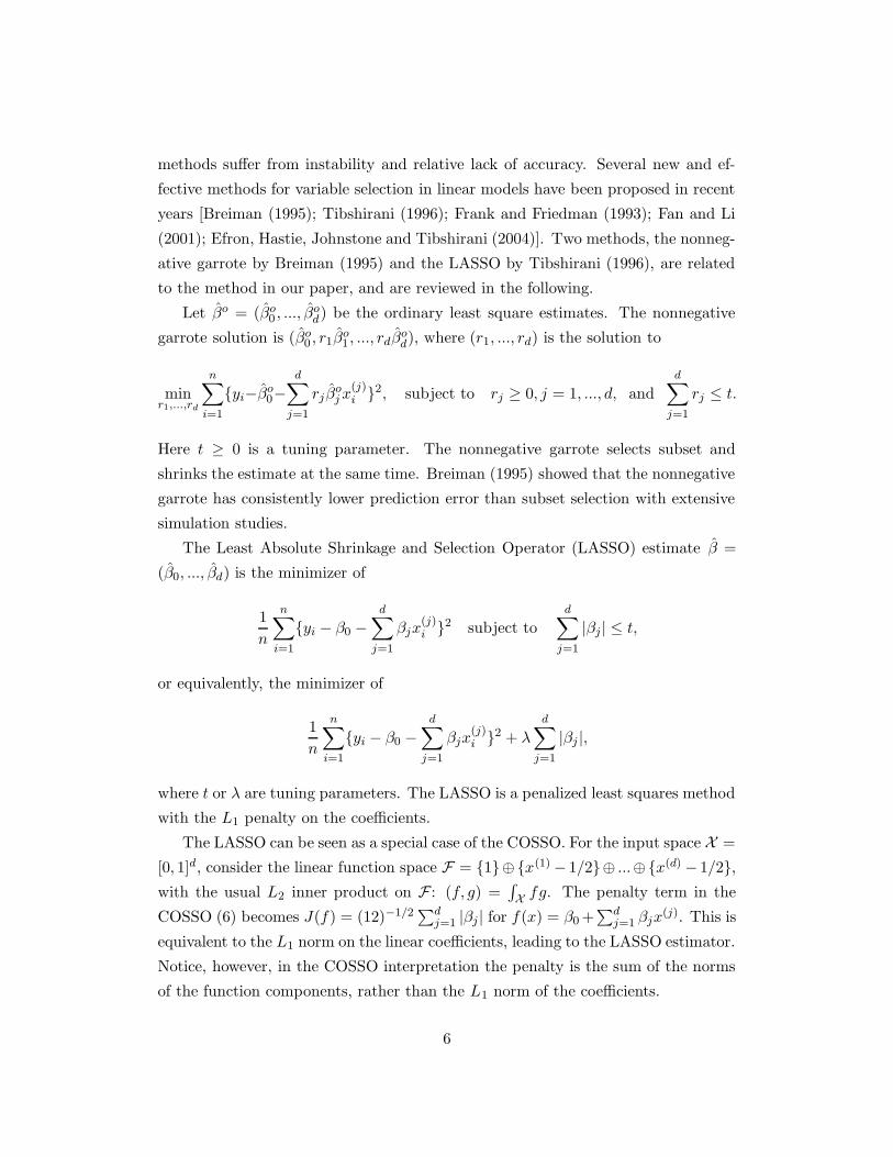
methods suffer from instability and relative lack of accuracy. Several new and ef-

fective methods for variable selection in linear models have been proposed in recent

years [Breiman (1995); Tibshirani (1996); Frank and Friedman (1993); Fan and Li

(2001); Efron, Hastie, Johnstone and Tibshirani (2004)]. Two methods, the nonneg-

ative garrote by Breiman (1995) and the LASSO by Tibshirani (1996), are related

to the method in our paper, and are reviewed in the following.

Let βo = (βo0 , ..., βo

d) be the ordinary least square estimates. The nonnegative

garrote solution is (βo0 , r1β

o1 , ..., rdβ

od), where (r1, ..., rd) is the solution to

minr1,...,rd

n∑

i=1

{yi−βo0−

d∑

j=1

rj βoj x

(j)i }2, subject to rj ≥ 0, j = 1, ..., d, and

d∑

j=1

rj ≤ t.

Here t ≥ 0 is a tuning parameter. The nonnegative garrote selects subset and

shrinks the estimate at the same time. Breiman (1995) showed that the nonnegative

garrote has consistently lower prediction error than subset selection with extensive

simulation studies.

The Least Absolute Shrinkage and Selection Operator (LASSO) estimate β =

(β0, ..., βd) is the minimizer of

1

n

n∑

i=1

{yi − β0 −d

∑

j=1

βjx(j)i }2 subject to

d∑

j=1

|βj | ≤ t,

or equivalently, the minimizer of

1

n

n∑

i=1

{yi − β0 −d

∑

j=1

βjx(j)i }2 + λ

d∑

j=1

|βj |,

where t or λ are tuning parameters. The LASSO is a penalized least squares method

with the L1 penalty on the coefficients.

The LASSO can be seen as a special case of the COSSO. For the input space X =

[0, 1]d, consider the linear function space F = {1}⊕{x(1) − 1/2}⊕ ...⊕{x(d) − 1/2},with the usual L2 inner product on F : (f, g) =

∫

Xfg. The penalty term in the

COSSO (6) becomes J(f) = (12)−1/2∑d

j=1 |βj | for f(x) = β0 +∑d

j=1 βjx(j). This is

equivalent to the L1 norm on the linear coefficients, leading to the LASSO estimator.

Notice, however, in the COSSO interpretation the penalty is the sum of the norms

of the function components, rather than the L1 norm of the coefficients.

6

2.4 Asymptotic property of the COSSO

In this section we assume a fixed design. Define y = (y1, ..., yn)T. With a little abuse

of notations, let f stand for both the regression function and its functional values at

data points, i.e., f = (f(x1), ..., f(xn))T. Define the norm ‖ · ‖n and inner product

〈·, ·〉n in Rn as

‖f‖2n =

1

n

n∑

i=1

f2(xi), 〈f, g〉n =1

n

n∑

i=1

f(xi)g(xi);

then ‖y − f‖2n = 1/n

∑ni=1{yi − f(xi)}2. The following theorem shows that the

COSSO estimator in the additive model has a rate of convergence n−`/(2`+1), where

` is the order of smoothness of the components.

Theorem 2 Consider the regression model yi = f0(xi) + εi, i = 1, ..., n, where xi’s

are given covariates in [0, 1]d, and εi’s are independent N(0, σ2) noises. Assume

f0 lies in F = {1} ⊕ F1, F1 =⊕d

j=1 Sj, with Sj = {1} ⊕ Sj being the `-th or-

der Sobolev space with norm (3). Consider the COSSO estimate f as defined in

(6). Then (i) if f0 is not a constant, and τ−1n = Op(n

`/(2`+1))J (2`−1)/(4`+2)(f0), we

have ‖f − f0‖n = Op(τn)J1/2(f0); (ii) if f0 is a constant, we have ‖f − f0‖n =

Op(max{n−`/(2`−1)τ−2/(2`−1)n , n−1/2}).

3 An equivalent formulation

It can be shown that the solution to (6) is in a finite dimensional space, therefore

the COSSO estimate can be computed directly from (6).

Lemma 1 Let f = b +∑p

α=1 fα be a minimizer of (6) in (4), with fα ∈ Fα. Then

fα ∈ span{Rα(xi, ·), i = 1, ..., n}, where Rα(·, ·) is the reproducing kernel of Fα.

However, it is possible to give an equivalent form of (6) that is easier to compute.

Consider the problem of finding θ = (θ1, ..., θp)T and f ∈ F to minimize

1

n

n∑

i=1

{yi − f(xi)}2 + λ0

p∑

α=1

θ−1α ‖P αf‖2 + λ

p∑

α=1

θα, subject to θα ≥ 0, α = 1, ..., p,

(8)

where λ0 is a constant and λ is a smoothing parameter. The constant λ0 can be fixed

at any positive value and is included here only for computational considerations.

7

Lemma 2 Set λ = τ 4/(4λ0). (i) If f minimizes (6), set θα = λ1/20 λ−1/2‖P αf‖, then

the pair (θ, f) minimizes (8). (ii) On the other hand, if a pair (θ, f) minimizes (8),

then f minimizes (6).

The form of (8) is very similar to the common smoothing spline (5) with mul-

tiple smoothing parameters, except that there is an additional penalty on the θ’s.

Different from Zhang et al. (2004) where the sparsity in coefficients does not assure

the sparsity in the functional components, for the COSSO procedure the sparsity of

each component fj is controlled by a single parameter θj. The additional penalty

term on θ’s,∑p

j=1 θj, shrinks them toward zero and hence makes θ’s sparse, giving

rise to zero function components in the COSSO estimate.

We only need to tune λ in the implementation of the COSSO, and λ0 can be

fixed at any positive value. In Section 6, we will see that an appropriate choice of

λ0 helps to put the tuning parameter on a natural scale and facilitates the tuning

of the COSSO. In contrast, the common smoothing spline has two sets of smooth-

ing parameters λ and θ’s that are confounded. The common way to search for

smoothing parameters iterates between λ and log θ’s, making it difficult to have

zero components in the solution.

4 A special case with the tensor product design

To illustrate the mechanism of the COSSO for model selection, in this section we

give an instructive analysis in the special case of a tensor product design with a SS-

ANOVA model built from the second order Sobolev spaces of periodic functions. We

assume the ε’s in the regression model are independent with distribution N(0, σ2).

In a tensor product design the design points are

{(xi1,1, xi2,2, ..., xid ,d) : ik = 1, ..., nk, k = 1, ..., d},

where xj,k = j/nk, j = 1, ..., nk, k = 1, ..., d. Without loss of generality, we fix

λ0 = 1 in the COSSO (8) and focus on the case of d = 2 with the SS-ANOVA model

being f(s, t) = b + f1(s) + f2(t) + f12(s, t). We assume n1 = n2 = m being an even

integer. The sample size is then n = m2.

The second order Sobolev space of periodic functions can be written as T =

8

{1} ⊕ T , where

T = {f : f(t) =

∞∑

ν=1

aν

√2 cos 2πνt+

∞∑

ν=1

bν

√2 sin 2πνt, with

∞∑

ν=1

(a2ν+b2

ν)(2πν)4 < ∞}.

The norm in T is ‖g‖2 =∫ 10 {g′′(t)}2 dt. When m is large, a good approximate

subspace of T is Tm = {1} ⊕ Tm with

Tm = {f : f(t) =

m/2−1∑

ν=1

aν

√2 cos 2πνt +

m/2−1∑

ν=1

bν

√2 sin 2πνt + am/2 cosπmt}.

Wahba (1990) used this subspace approximation to give a very instructive investiga-

tion of the filtering properties of the smoothing spline. Here we consider minimizing

(8) in Fm = T 1m ⊗ T 2

m = {1} ⊕ T 1m ⊕ T 2

m ⊕ (T 1m ⊗ T 2

m), as the argument is instruc-

tive. The argument for the more general function space F = T 1 ⊗ T 2 is similar but

involves more technicality, and is deferred to Appendix 2.

In this case (8) becomes

1

n

m∑

k=1

m∑

`=1

{ykl − f(xk,1, x`,2)}2 + θ−11

∫ 1

0

{

∂2f1(s)

∂s2

}2

ds + θ−12

∫ 1

0

{

∂2f2(t)

∂t2

}2

dt

+θ−112

∫ 1

0

∫ 1

0

{

∂4f12(s, t)

∂s2∂t2

}2

dsdt + λ(θ1 + θ2 + θ12), θ1 ≥ 0, θ2 ≥ 0, θ12 ≥ 0.

Write γ1(t) = 1, γ2ν(t) =√

2 cos(2πνt), γ2ν+1(t) =√

2 sin(2πνt), for ν =

1, ...,m/2 − 1, and γm(t) = cos(πmt). Then any function in Tm can be written

as g(t) =∑m

ν=1 aνγν(t), and any function in Fm can be written as

f(s, t) =

m∑

µ=1

m∑

ν=1

aµνγµ(s)γν(t). (9)

It is known that (see Wahba (1990), page 23)

m−1m

∑

k=1

γµ(k/m)γν(k/m) = 1 if µ = ν = 1, ...,m;

= 0 if µ 6= ν, µ, ν = 1, ...,m.

Recall the inner product 〈·, ·〉n of Rn defined in Section 2.4. Write γµν(s, t) =

9

γµ(s)γν(t), and γµν as the data vector corresponding to the function γµν(s, t). From

the above orthogonality relations and the tensor product design, we get

〈γµ1ν1, γµ2ν2

〉n = 1 if µ1 = µ2 = 1, ...,m; ν1 = ν2 = 1, ...,m;

= 0 if µ1 6= µ2 or ν1 6= ν2, µ1, ν1, µ2, ν2 = 1, ...,m.

Therefore {γµν , µ = 1, ...,m; ν = 1, ...,m} form an orthonormal basis in Rn with

respect to the norm ‖ · ‖n. We then get from (9) that aµν = 〈f, γµν〉n. Write

zµν = 〈y, γµν〉n. Then zµν = aµν + δµν , where δµν ∼ N(0, σ2/n) are independent.

The COSSO problem can be written as

m∑

µ=1

m∑

ν=1

(zµν−aµν)2+θ−11

m∑

µ=2

qµ1a2µ1+θ−1

2

m∑

ν=2

q1νa21ν+θ−1

12

m∑

µ=2

m∑

ν=2

qµνa2µν+λ(θ1+θ2+θ12),

(10)

with qµν ∼ µ4ν4 uniformly for µ 6= 1 or ν 6= 1, µ, ν = 1, ...,m. Here ∼ is read as

“has the same order as.” Therefore the minimizing aµν satisfies a11 = z11; aµ1 =

zµ1θ1(θ1 + qµ1)−1, for µ ≥ 2; a1ν = z1νθ2(θ2 + q1ν)

−1, for ν ≥ 2; aµν = zµνθ12(θ12 +

qµν)−1, for µ ≥ 2, ν ≥ 2; and (10) becomes

{m

∑

µ=2

qµ1z2µ1(qµ1 + θ1)

−1 + λθ1} + {m

∑

ν=2

q1νz21ν(q1ν + θ2)

−1 + λθ2}

+ {m

∑

µ=2

m∑

ν=2

qµνz2µν(qµν + θ12)

−1 + λθ12}.

We see that the three components can be minimized separately. Let us concentrate

on θ12, as θ1 and θ2 can be dealt with similarly. Let

A(θ12) =

m∑

µ=2

m∑

ν=2

qµνz2µν(qµν + θ12)

−1 + λθ12.

Then A′(θ12) = λ − ∑mµ=2

∑mν=2 qµνz

2µν(qµν + θ12)

−2, which increases as θ12 ≥ 0

increases. Define U =∑m

µ=2

∑mν=2 q−1

µν z2µν . If U ≤ λ, then A′(0) ≥ 0, A′(θ12) > 0

for all θ12 > 0, and the minimizing θ12 of A is 0; otherwise the minimizing θ12 is

larger than 0. Therefore we can see that the COSSO estimator selects components

through a soft thresholding type operation according to the magnitude of U . Notice

θ12 = 0 implies f12 = 0.

10

With the analysis above, we can now show that, when λ → 0 and nλ → ∞, the

COSSO selects the correct model with probability tending to one. Without loss of

generality, let us concentrate on f12.

If f12 = 0, then aµν = 0 for any pair (µ, ν) such that µ ≥ 2 and ν ≥ 2. So

E(U) ∼ σ2/n∑m

µ=2

∑mν=2 µ−4ν−4 ∼ n−1σ2, var(U) =

∑mµ=2

∑mν=2 2n−2σ4q−2

µν ∼n−2σ4. Therefore when nλ → ∞, by Chebyshev’s inequality,

pr(U > λ) ≤ pr(|U − E(U)| > λ − E(U)) ≤ var(U)/{λ − E(U)}2 → 0.

Therefore with probability tending to unity, U ≤ λ, and thus f12 = 0.

On the other hand, if f12 6= 0, then aµ0,ν06= 0 for some µ0 ≥ 2 and ν0 ≥ 2, and

E(U) ≥ E(q−1µ0,ν0

z2µ0,ν0

) ≥ q−1µ0,ν0

a2µ0,ν0

;

var(U) =

m∑

µ=2

m∑

ν=2

q−2µν var(z2

µν) =

m∑

µ=2

m∑

ν=2

q−2µν (4n−1a2

µνσ2 + 2n−2σ4)

≤ {4n−1σ2m

∑

µ=2

m∑

ν=2

a2µν} + 2n−2σ4 = 4n−1σ2‖f12‖2

L2+ 2n−2σ4 = O(n−1).

Therefore when λ → 0, by Chebyshev’s inequality, we get

pr(U < λ) ≤ pr(|U − E(U)| > E(U) − λ) ≤ var(U)/{E(U) − λ}2 → 0.

Therefore with probability tending to unity, U > λ, and thus f12 6= 0.

5 Algorithm

For any fixed θ, the COSSO (8) is equivalent to the smoothing spline (5). Therefore

from the smoothing spline literature [for example,Wahba (1990)] it is well known

the solution f has the form f(x) =∑n

i=1 ciRθ(xi, x) + b, where c = (c1, ..., cn)T ∈Rn, b ∈ R, and Rθ =

∑pα=1 θαRα, with Rα being the reproducing kernel of Fα.

With some abuse of notations, let Rα also stand for the n × n matrix {Rα(xi, xj)},i = 1, ..., n, j = 1, ..., n, let Rθ also stand for the matrix

∑pα=1 θαRα, and let 1r be

the column vector consisting of r ones. Then we can write f = Rθc + b1n, and (8)

11

can be expressed as

1

n(y −

p∑

α=1

θαRαc − b1n)T(y −p

∑

α=1

θαRαc − b1n) + λ0

p∑

α=1

θαcTRαc + λ

p∑

α=1

θα, (11)

where θα ≥ 0, α = 1, ..., p.

If θ’s were fixed, then (11) can be written as

minc,b

(y − Rθc − b1n)T(y − Rθc − b1n) + nλ0cTRθc. (12)

The solution to this smoothing spline problem is given in Wahba (1990).

On the other hand, if c and b were fixed, denote gα = Rαc, and let G be the

n × p matrix with the αth column being gα. Simple calculation shows that the

θ = (θ1, ..., θp)T that minimizes (11) is the solution to

minθ

(z − Gθ)T(z − Gθ) + nλ

p∑

α=1

θα subject to θα ≥ 0, α = 1, ..., p, (13)

where z = y − (1/2)nλ0c − b1n.

Therefore a reasonable scheme would be to iterate between (12) and (13). In

each iteration (11) is decreased. Notice that (13) is equivalent to

minθ

(z − Gθ)T(z − Gθ) subject to θα ≥ 0, α = 1, ..., p;

p∑

α=1

θα ≤ M, (14)

for some M ≥ 0. We prefer to iterate between (12) and (14) for computational

considerations.

Notice that the formulation (14) is exactly the problem in calculating the non-

negative garrote estimate. Therefore our algorithm iterates between the smoothing

spline and the nonnegative garrote. The algorithm starts with a natural initial solu-

tion given by the smoothing spline, which is already a good estimate. By applying

later iterations of our algorithm, we get what we view as an iterative improvement

on the smoothing spline. A limited number of iterations are usually sufficient to

achieve good performance in practical applications. This is in spirit similar to the

basis pursuit algorithm in Chen, Donoho and Saunders (1998). We observe empir-

ically that the COSSO objective function decreases quickly in the first iteration,

12

and the objective function after the first iteration is already very close to the objec-

tive function at convergence, as the magnitude of the decrease in the first iteration

dominates the decreases in subsequent iterations. This motivates us to consider the

following one step update procedure:

1. Initialization: Fix θα = 1, α = 1, ..., p.

2. Solve for c and b with (12).

3. For c and b obtained in step 2, solve for θ with the nonnegative garrote (14).

4. With the new θ, solve for c and b with the smoothing spline (12).

This one step update procedure has the flavor of the one step maximum likeli-

hood procedure, in which one step Newton-Raphson algorithm is applied to a good

initial estimator and which is as efficient as the fully iterated maximum likelihood.

A discussion of one step procedure and fully iterated procedure (in a different algo-

rithm) can be found in Fan and Li (2001). In our experience, the one step update

procedure and the fully iterated procedure have comparable estimation accuracy.

6 Choosing the tuning parameter

The generalized cross validation proposed by Craven and Wahba (1979) is one of the

most popular methods for choosing smoothing parameters in the smoothing spline

method. Let A be the smoothing matrix of the smoothing spline. That is, y = Ay.

The generalized cross validation estimate of the risk is

GCV =‖y − y‖2

n

{n−1tr(I − A)}2.

Tibshirani (1996) proposed a GCV-type criterion for choosing the tuning param-

eter for the LASSO through a ridge estimate approximation. This approximation

is particularly easy to understand in light of the form (8) for the linear model

f(x) = β0 +∑d

j=1 βjx(j): fix the θj’s at their estimated values θj’s, and calcu-

late GCV for the corresponding ridge regression. This approximation ignores some

variability in the estimation process. However, the simulation study in Tibshirani

(1996) suggests that it is a useful approximation. This motivates our GCV-type

13

criterion: We use the GCV score for the smoothing spline in (8) when θ’s are fixed

at the solution.

Another popular technique for choosing tuning parameters is the five or ten

fold cross validation. The computation load of GCV is smaller. We compare the

performances of these two criteria in the COSSO with simulations. It is also possible

to use the Cp criterion based on the concept of generalized degrees of freedom (Ye

(1998); Shen and Ye (2002)). We do not consider this possibility since in our problem

there is no explicit formula for the degrees of freedom and numerical evaluations tend

to be computationally intensive.

The following is the complete algorithm for the COSSO with adaptive tuning:

1. Fix θα = 1, α = 1, ..., p. Solve the smoothing spline problem, and tune λ0

according to CV or GCV. Fix λ0 at the chosen value in all later steps.

2. For each fixed M in a reasonable range, apply the one step COSSO algo-

rithm with M . Choose the best M according to CV or GCV. The solution

corresponding to this chosen M is the final solution.

In our simulations, it is noticed that once λ0 is fixed according to step 1, the

optimal M seems to be close to the number of important components. This helps

for determining the range of tuning for M .

7 Simulations

In this section we study the empirical performance of the COSSO estimate in terms

of estimation accuracy and model selection. We compare the COSSO with GCV,

the COSSO with five-fold cross validation, and MARS, which is a popular stepwise

forward/backward procedure for building functional ANOVA models. The measure

of accuracy is the integrated squared error ISE = EX{f(X) − f(X)}2, which is

estimated by Monte Carlo integration using 10, 000 test points from the same dis-

tribution as the training points. We run each simulation example 100 times and

average. The matlab code for the COSSO is available from webpages of the authors

(www.stat.wisc.edu/˜yilin or www4.stat.ncsu.edu/˜hzhang). The MARS simula-

tions are done in R, with the function “mars” in the “mda” library contributed by

Trevor Hastie and Robert Tibshirani.

14

The following four functions on [0, 1] are used as building blocks of regression

functions in some of the simulations: g1(t) = t; g2(t) = (2t−1)2; g3(t) = sin(2πt)2−sin(2πt) ;

and g4(t) = 0.1 sin(2πt) + 0.2 cos(2πt) + 0.3 sin2(2πt) + 0.4 cos3(2πt) + 0.5 sin3(2πt).

Consider two covariance structures of the input vector X, with varying correlation:

Compound symmetry: Let X (j) = (Wj + tU)/(1 + t), j = 1, ..., d, where W1, ...,

Wd and U are i.i.d from Uniform(0,1). Therefore corr(X (j), X(k)) = t2/(1+t2)

for j 6= k. The uniform design corresponds to the case t = 0.

(trimmed) AR(1): Let W1, ..., Wd be i.i.d N(0, 1), and X (1) = W1, X(j) =

ρX(j−1) +(1−ρ2)1/2Wj, j = 2, ..., d. Trim X (j) in [-2.5, 2.5] and scale to [0,1].

Example 1. Consider a simple additive model in R10, with the underlying re-

gression function f(x) = 5g1(x(1)) + 3g2(x

(2)) + 4g3(x(3)) + 6g4(x

(4)). Therefore

X(5), ..., X(10) are uninformative. We consider a sample size n = 100. Generate

y = f(x) + ε, where ε is distributed as N(0, 1.74). The standard deviation of the

noise was chosen to give a signal to noise ratio 3 : 1 in the uniform case. For

comparison, the variances of the component functions are var{5g1(X(1))} = 2.08,

var{3g2(X(2))} = 0.80, var{4g3(X

(3))} = 3.30 and var{6g4(X(4))} = 9.45.

0 1 2 3 4 5 6 7 80

0.5

1

1.5

2

2.5

3

x4

x3

x1

x2

x7

The tuning parameter M

The

empi

rical

L1 n

orm

of t

he c

ompo

nent

s

Figure 1: The empirical L1 norm of the estimated components as plotted against

the tuning parameter M in one run of Example 1.

15

We apply the COSSO with additive models (the additive COSSO) to the sim-

ulated data. Therefore there are 10 functional components in the model. Figure 1

shows how the magnitudes of the estimated components change with the tuning pa-

rameter M in one run. The magnitudes of the functional components are measured

by their empirical L1 norms, defined as 1/n∑n

i=1 |fj(x(j)i )| for j = 1, ..., d. The λ0

in this run is fixed at 9.7656×10−6 . Both GCV and five-fold cross validation choose

M = 3.5, giving a model of 5 terms in this run. The estimated function compo-

nents are plotted along with the true function components in Figure 2. Notice the

components are centered according to the ANOVA decomposition.

0 0.5 1−5

0

5

x1

0 0.5 1−5

0

5

x2

0 0.5 1−5

0

5

x3

0 0.5 1−5

0

5

x4

0 0.5 1−5

0

5

x7

Figure 2: The estimated component (dashed line) and true component (solid line)

functions in one run of Example 1. Shown are the components for variables 1, 2, 3,

4, and 7. For the other variables, both true and estimated components are zero.

For each setting of covariance structure, we run the simulation 100 times and

average. The resulting average integrated squared error and its associated standard

error (in parentheses) are given in Table 1. Also included in the table is the average

integrated squared error of MARS for additive models. We can see the two COSSO

procedures perform better than MARS in all the settings studied. To study the

performance of the COSSO in terms of model selection, we determine in the uniform

16

case the number of times each variable appears in the 100 chosen models (Table 2),

and the number of terms in the 100 chosen models (Table 3). In our calculation

we take θ to be zero if it is smaller than 10−6. The COSSO with five-fold cross

validation misses the second variable 6 times, but chooses the correct four variable

model 84 times. The COSSO with GCV and the MARS do not miss any important

variable, but tend to include uninformative variables in the chosen models. The

COSSO with GCV chooses the correct four variable model 57 times, while MARS

does that only 4 times.

Table 1. Comparison of average integrated squared errors for Example 1.

Comp. symm. AR(1)

t = 0 t = 1 t = 3 ρ = −0.5 ρ = 0 ρ = 0.5

COSSO(GCV) 0.93 (0.05) 0.92 (0.04) 0.97 (0.07) 0.94 (0.05) 1.04 (0.07) 0.98 (0.07)

COSSO(5CV) 0.80 (0.03) 0.97 (0.05) 1.07 (0.06) 1.03 (0.06) 1.03 (0.06) 0.98 (0.05)

MARS 1.57 (0.07) 1.24 (0.06) 1.30 (0.06) 1.32 (0.07) 1.34 (0.07) 1.36 (0.08)

Table 2. Appearance frequency of the variables in the models in the uniform

setting.

Variable

1 2 3 4 5 6 7 8 9 10

COSSO(GCV) 100 100 100 100 14 11 18 15 11 13

COSSO(5CV) 100 94 100 100 1 1 3 2 4 2

MARS 100 100 100 100 35 35 34 39 28 35

Table 3. Frequency of the size of the models in the uniform setting.

Model size

3 4 5 6 7 8 9 10 Mean

COSSO(GCV) 0 57 17 18 5 2 0 1 4.82

COSSO(5CV) 6 84 7 3 0 0 0 0 4.07

MARS 0 4 24 40 26 6 0 0 6.06

Table 4 gives the mean and standard deviation of the model sizes chosen by the

methods in various settings. The settings considered are compound symmetry with

17

t = 1 and 3 and trimmed AR(1) with ρ = −0.5, 0 and 0.5. The average model size

chosen by the COSSO with five-fold cross validation is close to 4, the size of the true

model. The COSSO with GCV selects slightly larger models. The models chosen

by MARS are even larger.

Table 4. Mean and standard deviation of the model sizes.Comp. symm. AR(1)

t = 1 t = 3 ρ = −0.5 ρ = 0 ρ = 0.5

COSSO(GCV) 4.8 (1.2) 4.8 (1.5) 4.7 (1.2) 4.8 (1.3) 4.6 (1.2)

COSSO(5CV) 4.1 (1.2) 4.4 (1.9) 4.1 (1.2) 4.0 (1.0) 3.8 (0.9)

MARS 6.3 (0.9) 6.2 (0.9) 6.1 (1.0) 6.1 (0.8) 5.9 (0.8)

Example 2. Consider a larger model with d = 60, and the regression function

f(x) = g1(x(1)) + g2(x

(2)) + g3(x(3)) + g4(x

(4)) + 1.5g1(x(5)) + 1.5g2(x

(6))

+ 1.5g3(x(7)) + 1.5g4(x

(8)) + 2g1(x(9)) + 2g2(x

(10)) + 2g3(x(11)) + 2g4(x

(12)).

Therefore there are 48 uninformative variables. Let n = 500. The variance of the

normal noise is 0.5184, to give a signal to noise ratio of 3 : 1 in the uniform case.

For comparison, in the uniform setting var{g1(X(1))} = 0.08, var{g2(X

(2))} = 0.09,

var{g3(X(3))} = 0.21 and var{g4(X

(4))} = 0.26. Both COSSO and MARS are run

100 times with additive models. The results are summarized in Table 5. We see

that the two COSSO procedures outperform MARS, with the COSSO with five-fold

cross validation doing slightly better than the COSSO with GCV.

Table 5. Average ISE (unit 10−3) and model sizes with their standard errors.

Comp. symm. AR(1)

t = 0 t = 1 ρ = 0.5 ρ = −0.5

ISE COSSO(GCV) 201 (4) 178 (5) 199 (6) 183 (5)

COSSO(5CV) 144 (4) 162 (5) 153 (4) 149 (5)

MARS 353 (7) 302 (7) 286 (6) 280 (5)

Model Sizes COSSO(GCV) 18.0 (4.1) 18.0 (4.1) 19.0 (5.1) 18.0 (4.3)

COSSO(5CV) 12.0 (0.2) 11.7 (1.4) 12.1 (1.4) 11.9 (1.0)

MARS 35.2 (2.3) 36.1 (2.1) 35.2 (2.5) 35.9 (2.4)

18

Example 3. We consider a 10 dimensional regression problem with several two

way interactions:

f(x) = g1(x(1))+g2(x

(2))+g3(x(3))+g4(x

(4))+g1(x(3)x(4))+g2(

x(1) + x(3)

2)+g3(x

(1)x(2)).

We consider the uniform setting, and set the noise to be normal with standard

deviation 0.2546, to give a signal to noise ratio of 3 : 1. The average integrated

squared errors are given in Table 6 for sample sizes n = 100, 200, 400. Both the

COSSO and MARS are run with the two way interaction model. We follow the

advice in Friedman (1991) to set the cost for each basis function optimization to be

3 in the MARS for two way interaction models.

Table 6. Average integrated squared errors for Example 3.

n = 100 n = 200 n = 400

COSSO(GCV) 0.358 (0.009) 0.100 (0.003) 0.045 (0.001)

COSSO(5CV) 0.378 (0.005) 0.094 (0.004) 0.043 (0.001)

MARS 0.239 (0.008) 0.109 (0.003) 0.084 (0.001)

There are 55 function components in the COSSO. The COSSO does not do

well when n = 100. It seems that there are too many function components for

the COSSO to select from with 100 data points. MARS does not suffer from a

small sample size so much as the COSSO. Part of the reason is that the MARS

algorithm introduces a certain hierarchical order of the terms being searched from:

only after a univariate basis function is included in the model, will the product of

other terms with it become a candidate for inclusion in later steps. In contrast, the

COSSO selects from all the function components and does not distinguish between

main effects and interaction terms. Therefore the COSSO does not assume any

hierarchical structure, and may not be efficient when the true model is hierarchical

and the sample size is small. However, as the sample size increases, the COSSO

procedures catch up quickly. Their performances are comparable to MARS when

n = 200 and better than MARS when n = 400.

In the above examples we see that in general the COSSO with five-fold cross

validation tends to do better than the COSSO with the GCV. We therefore recom-

mend the use of five-fold cross validation with the COSSO unless the computation

19

time is a crucial factor. In the following examples the COSSO is tuned with five-fold

cross validation.

Example 4. The circuit example. This is an example from Friedman (1991).

Of interest is the dependence of the impedance Z of a circuit and phase shift φ on

components in the circuit. The true dependence is described by

Z = [R2 + {ωL − 1/(ωC)}2]1/2,

φ = tan−1{ωL − 1/(ωC)

R

}

.

The input variables are uniform in the range: 0 ≤ R ≤ 100, 40π ≤ ω ≤ 560π, 0 ≤L ≤ 1, 1 ≤ C ≤ 11, and the noise is normal with the standard deviation set to give

a signal to noise level 3 : 1.

This is a relatively small problem with d = 4. All order of interactions are

present. Friedman (1991) applied MARS with additive model, two way interaction

model, and the saturated model to this example, and found that the performance

of the two way interaction model was the best. We scale the input region to [0, 1]4

and apply the COSSO with five fold cross validation. With the small dimension, it

is possible to apply the COSSO with the saturated model, which has 24 − 1 = 15

function components. However, it turns out that the two way interaction COSSO

does slightly better than the saturated model. We compare the integrated squared

error of the two way interaction COSSO and that of the two way interaction MARS

in Table 7. It turns out that the COSSO performs much better than MARS. We note

that in Table 7, the numbers reported for the MARS when n = 200 are calculated

after excluding one large extreme outlier in ISE, and those for the MARS when

n = 400 are calculated after excluding three large extreme outliers in ISE.

Table 7. Average integrated squared errors for estimating the impedance Z (in the

unit of 103) and the phase shift φ (in the unit of 10−3).

n = 100 n = 200 n = 400

For Z COSSO 1.91 (0.12) 0.85 (0.05) 0.51 (0.03)

MARS 5.57 (0.41) 2.47 (0.16) 1.37 (0.08)

For φ COSSO 12.98 (0.36) 7.96 (0.20) 5.36 (0.10)

MARS 20.59 (0.96) 12.60 (0.71) 8.19 (0.14)

20

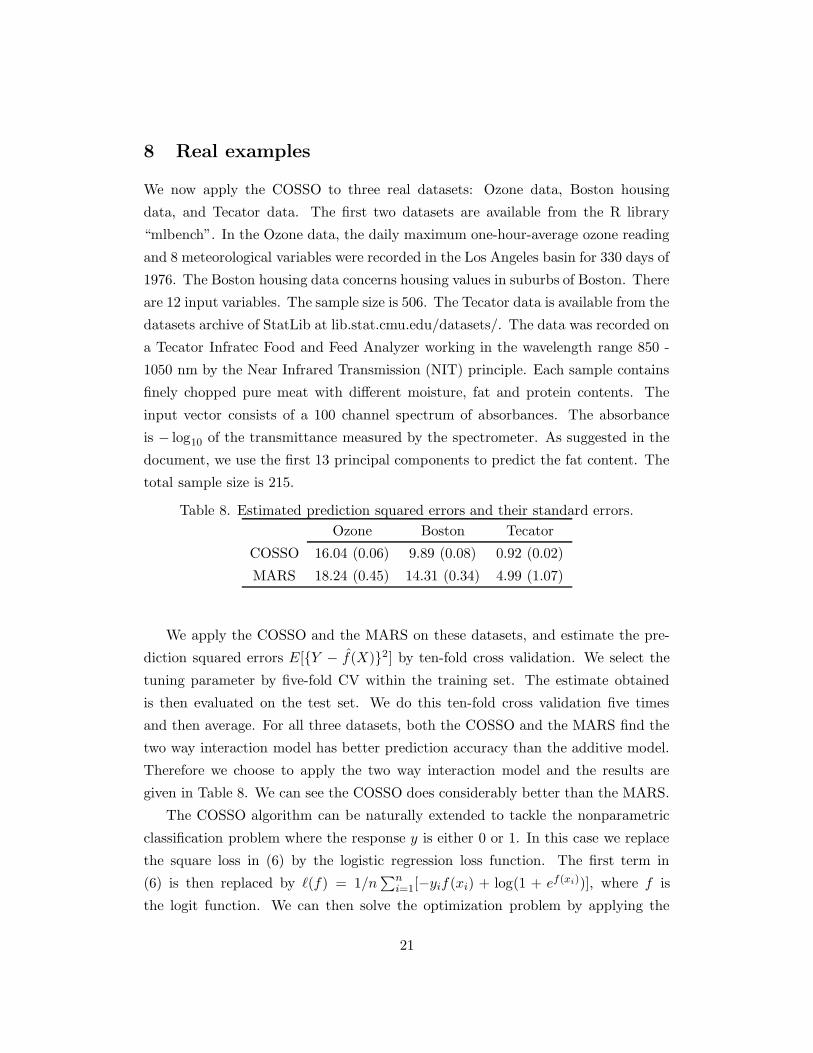
8 Real examples

We now apply the COSSO to three real datasets: Ozone data, Boston housing

data, and Tecator data. The first two datasets are available from the R library

“mlbench”. In the Ozone data, the daily maximum one-hour-average ozone reading

and 8 meteorological variables were recorded in the Los Angeles basin for 330 days of

1976. The Boston housing data concerns housing values in suburbs of Boston. There

are 12 input variables. The sample size is 506. The Tecator data is available from the

datasets archive of StatLib at lib.stat.cmu.edu/datasets/. The data was recorded on

a Tecator Infratec Food and Feed Analyzer working in the wavelength range 850 -

1050 nm by the Near Infrared Transmission (NIT) principle. Each sample contains

finely chopped pure meat with different moisture, fat and protein contents. The

input vector consists of a 100 channel spectrum of absorbances. The absorbance

is − log10 of the transmittance measured by the spectrometer. As suggested in the

document, we use the first 13 principal components to predict the fat content. The

total sample size is 215.

Table 8. Estimated prediction squared errors and their standard errors.

Ozone Boston Tecator

COSSO 16.04 (0.06) 9.89 (0.08) 0.92 (0.02)

MARS 18.24 (0.45) 14.31 (0.34) 4.99 (1.07)

We apply the COSSO and the MARS on these datasets, and estimate the pre-

diction squared errors E[{Y − f(X)}2] by ten-fold cross validation. We select the

tuning parameter by five-fold CV within the training set. The estimate obtained

is then evaluated on the test set. We do this ten-fold cross validation five times

and then average. For all three datasets, both the COSSO and the MARS find the

two way interaction model has better prediction accuracy than the additive model.

Therefore we choose to apply the two way interaction model and the results are

given in Table 8. We can see the COSSO does considerably better than the MARS.

The COSSO algorithm can be naturally extended to tackle the nonparametric

classification problem where the response y is either 0 or 1. In this case we replace

the square loss in (6) by the logistic regression loss function. The first term in

(6) is then replaced by `(f) = 1/n∑n

i=1[−yif(xi) + log(1 + ef(xi))], where f is

the logit function. We can then solve the optimization problem by applying the

21

quadratic approximation to `(f) iteratively. This leads to the iteratively reweighted

least squares (IRLS) procedure, which is equivalent to a Newton-Raphson algorithm.

Using this approach, we can solve our optimization problem by iterative application

of the COSSO algorithm, within an IRLS loop. We illustrate the performance of

this procedure by comparing it with a number of machine learning algorithms on

several high dimensional real data sets.

Table 9: Comparison of the test set performance of the COSSO with the

performances of SVM, LS-SVM, LDA, QDA, Logit, C4.5, oneR, IB, Naive Bayes,

and the Majority Rule.

BUPA Ionosphere Pima Indian Sonar MR Wisc. BC

n 345 351 768 208 683

d 6 33 8 60 9

COSSO 71.1 (3.5) 91.1 (3.7) 77.3 (2.2) 79.0 (4.5) 97.0 (0.8)

SVM (linear) 67.7 (2.6) 87.1 (3.4) 77.0 (2.4) 74.1 (4.2) 96.3 (1.0)

SVM (RBF) 70.4 (3.2) 95.4 (1.7) 77.3 (2.2) 75.0 (6.6) 96.4 (1.0)

LS-SVM (linear) 65.6 (3.2) 87.9 (2.0) 76.8 (1.8) 72.6 (3.7) 95.8 (1.0)

LS-SVM (RBF) 70.2 (4.1) 96.0 (2.1) 76.8 (1.7) 73.1 (4.2) 96.4 (1.0)

LDA 65.4 (3.2) 87.1 (2.3) 76.7 (2.0) 67.9 (4.9) 95.6 (1.1)

QDA 62.2 (3.6) 90.6 (2.2) 74.2 (3.3) 53.6 (7.4) 94.5 (0.6)

Logit 66.3 (3.1) 86.2 (3.5) 77.2 (1.8) 68.4 (5.2) 96.1 (1.0)

C4.5 63.1 (3.8) 90.6 (2.2) 73.5 (3.0) 72.1 (2.5) 94.7 (1.0)

oneR 56.3 (4.4) 83.6 (4.8) 71.3 (2.7) 62.6 (5.5) 91.8 (1.4)

IB 61.3 (6.2) 87.2 (2.8) 73.6 (2.4) 77.7 (4.4) 96.4 (1.2)

Naive Bayes 63.7 (4.5) 92.1 (2.5) 75.5 (1.7) 71.6 (3.5) 97.1 (0.9)

Majority Rule 56.5 (3.1) 64.4 (2.9) 66.8 (2.1) 54.4 (4.7) 66.2 (2.4)

Gestel et al. (2004) conducted a benchmark study comparing a number of com-

monly used machine learning techniques including the support vector machine (SVM);

least squares SVM (LS-SVM); linear discriminant analysis (LDA); quadratic dis-

criminant analysis (QDA); logistic regression (Logit); the decision tree algorithm

C4.5; Holte’s one-rule classifier (oneR); instance based learners (IB); and the Naive

Bayes method. There are five binary classification datasets with continuous predic-

tors, and we test the performance of the COSSO on these datasets. The datasets

22

are the BUPA Liver Disorder data, the Johns Hopkins University Ionosphere data;

the PIMA Indian Diabetes; the Sonar, Mines vs. Rocks data; and the Wisconsin

Breast Cancer data. The basic features of the datasets and the performances of

different algorithms are summarized in Table 9. Due to the high dimension of these

problems, we only consider the COSSO additive model.

Following Gestel et al. (2004), for each dataset we randomly select 2/3 of the

data for training and tuning, and test on the remaining 1/3 of the data. We do this

randomization 10 times and report the average test set performance and sample

standard deviation for the COSSO. The results for the other algorithms are taken

from Gestel et al. (2004). Gestel et al. (2004) included six types of LS-SVMs and

found that the LS-SVM with the radial basis function (RBF) kernel performs the

best overall. To save space we only include the LS-SVM with RBF kernel and linear

kernel in Table 9. Gestel et al. (2004) included two instance based learners (IB1

and IB10 in that paper). We combine them and report the better performance

of the two. Same is done for the two Naive Bayes methods considered in Gestel

et al. (2004). The best average test set performance is denoted in bold face for each

dataset in Table 9. We can see the COSSO gives very competitive performance on

these benchmark datasets.

9 Discussion

The difference between the COSSO and the common smoothing spline in smooth-

ing spline ANOVA mirrors that between the LASSO and ridge regression in linear

models. Compared with other model selection algorithms based on greedy search,

the COSSO optimizes a global criterion and provides a shrinkage estimate. We have

shown that the COSSO has attractive properties for model selection and estimation.

One future research topic is the statistical inference based on the COSSO. Tra-

ditionally inference after model selection is based on the selected models, resulting

in biased inferences. Shen et al. (2004) proposed a method to make approximately

unbiased inferences. It is of interest to see if their method can be adapted to our

problem to give unbiased inferences.

APPENDIX 1

Proof of Theorem 1. Denote the functional to be minimized in (6) by A(f),

23

then A(f) is convex and continuous. Without loss of generality, we assume τ = 1.

By (7) we have that J(f) ≥ ‖f‖, for any f ∈ F1. Let RF1be the reproducing

kernel of F1 and 〈·, ·〉F1be the inner product in F1. Denote a = maxn

i=1 R1/2F1

(xi, xi).

By the definition of reproducing kernel, we have for any f ∈ F1 and i = 1, ..., n,

|f(xi)| = |〈f(·), RF1(xi, ·)〉F1

| ≤ ‖f‖〈RF1(xi, ·), RF1

(xi, ·)〉1/2F1

= ‖f‖R1/2F1

(xi, xi) ≤ a‖f‖ ≤ aJ(f). (A1)

Denote ρ = maxni=1(y

2i + |yi| + 1). Consider the set

D = {f ∈ F : f = b + f1,with b ∈ {1}, f1 ∈ F1, J(f) ≤ ρ, |b| ≤ ρ1/2 + (a + 1)ρ}.

Then D is a closed, convex, and bounded set. Therefore by Theorem 4 of Tapia

and Thompson (1978, page 162), there exists a minimizer of (6) in D. Denote the

minimizer by f . Then A(f) ≤ A(0) < ρ.

On the other hand, for any f ∈ F with J(f) > ρ, clearly A(f) ≥ J(f) > ρ; for

any f ∈ F with J(f) ≤ ρ, f = b + f1, b ∈ {1}, f1 ∈ F , and |b| > ρ1/2 + (a + 1)ρ, we

use (A1) to get that, for any i = 1, ..., n,

|b + f1(xi) − yi| > [ρ1/2 + (a + 1)ρ] − aρ − ρ = ρ1/2.

Therefore A(f) > ρ. For any f 6∈ D, A(f) > A(f), i.e. f is a minimizer of (6) in F .

Proof of Theorem 2. For any f ∈ F , we can write f(x) = c + f1(x(1)) +

... + fd(x(d)) = c + g(x), such that

∑ni=1 fj(x

(j)i ) = 0, j = 1, ..., d. Similarly, write

f0(x) = c0 + f01(x(1)) + ... + f0d(x

(d)) = c0 + g0(x), and f(x) = c + f1(x(1)) + ... +

fd(x(d)) = c + g(x). By construction

∑ni=1{g0(xi) − g(xi)} = 0, we can write (6) as

(c0 − c)2 +2

n(c0 − c)

n∑

i=1

εi +1

n

n∑

i=1

{g0(xi) + εi − g(xi)}2 + τ2nJ(g).

Therefore, the minimizing c must minimize (c0 − c)2 +2/n(c0 − c)∑n

i=1 εi. That

is, c = c0 + 1/n∑n

i=1 εi. Therefore (c − c0)2 converges with rate n−1. On the other

hand, g must minimize

1

n

n∑

i=1

{g0(xi) + εi − g(xi)}2 + τ2nJ(g).

24

Let G = {g ∈ F : g(x) = f1(x(1)) + ... + fd(x

(d)), with∑n

i=1 fj(x(j)i ) = 0, j =

1, ..., d}. Then g0 ∈ G, g ∈ G. The conclusion of Theorem 2 then follows from

Theorem 10.2 of van de Geer (2000) and the following lemma.

Lemma 3 Let H∞(δ,G) be the δ-entropy of G for the supremum norm. Then

H∞(δ, {g ∈ G : J(g) ≤ 1}) ≤ Ad(`+1)/`δ−1/`,

for all δ > 0, n ≥ 1 and some A > 0 not depending on δ, n, or d.

Proof of Lemma 3. Define Gj as the set of univariate functions of x(j):

Gj = {fj ∈ S` : J(fj) ≤ 1,

n∑

i=1

fj(x(j)i ) = 0},

where S` is the `-th order Sobolev space. Then from (3), any h ∈ G j satisfies

`−2∑

ν=0

[h(ν)(1) − h(ν)(0)]2 +

∫ 1

0{h(`)(t)}2 dt ≤ 1. (A2)

We first show that for any h ∈ Gj , we have |h|∞ ≡ {sups∈[0,1] |h(s)|} ≤ 1. For

any fixed h ∈ Gj , define K = {k : 0 ≤ k ≤ `− 1, and for any integer q ∈ [0, k], there

exists aq ∈ [0, 1] satisfying h(q)(aq) = 0}. Since∑n

i=1 h(x(j)i ) = 0, we have 0 ∈ K.

Let k0 be the largest number in K. Now we consider two possibilities k0 6= ` − 1

and k0 = ` − 1 separately.

If k0 6= ` − 1, then k0 ≤ ` − 2, k0 ∈ K, and k0 + 1 6∈ K. By the definition of K,

we see that h(k0) is monotone, and crosses the x-axis. So for any s ∈ [0, 1], we have

|h(k0)(s)| ≤ |h(k0)(1) − h(k0)(0)| ≤ 1. The last inequality follows from (A2). From

this and the fact that h(k0−1) crosses the x-axis, we get |h(k0−1)(s)| ≤ 1, ∀s ∈ [0, 1].

Continuing with this argument, we get |h|∞ ≤ 1.

On the other hand, if k0 = `−1, then maxs h(`−1)(s) ≥ 0, and mins h(`−1)(s) ≤ 0.

By (A2) we get

1 ≥∫ 1

0{h(`)(t)}2dt ≥ {

∫ 1

0|h(`)(t)|dt}2 ≥ {max

sh(`−1)(s) − min

sh(`−1)(s)}2.

Therefore −1 ≤ mins h(`−1)(s) ≤ 0 ≤ maxs h(`−1)(s) ≤ 1. That is, |h(`−1)(s)| ≤ 1,

25

∀s ∈ [0, 1]. Now by the definition of K and that ` − 1 ∈ K, we know that h(k)

crosses the x-axis for any integer k ∈ [0, ` − 1]. Therefore we get |h|∞ ≤ 1.

Therefore we have shown that |h|∞ ≤ 1 for any h ∈ Gj . It then follows from

Theorem 2.4 of van de Geer (2000, page 19)that

H∞(δ,Gj) ≤ Aδ−1/` (A3)

for all δ > 0, and n ≥ 1, and some positive A not depending on δ and n.

By the definition of the G and Gj , we see that in terms of the supreme norm,

if each Gj , j = 1, ...d, can be covered by N balls of radius δ, then the set {g ∈ G :

J(g) ≤ 1} can be covered by N d balls with radius dδ. By (A3) we get

H∞(dδ, {g ∈ G : J(g) ≤ 1}) ≤ Adδ−1/`,

and the conclusion of the lemma follows.

Proof of Lemma 1. For any f ∈ F , we can write f = b +∑p

α=1 fα with

fα ∈ Fα. Let the projection of fα onto span{Rα(xi, ·), i = 1, ..., n} ⊂ Fα be gα and

its orthogonal complement be hα. Then fα = gα + hα, and ‖fα‖2 = ‖gα‖2 + ‖hα‖2,

α = 1, ..., p. Since R = 1+∑p

α=1 Rα is the reproducing kernel of F , we have, making

use of the orthogonal structures,

f(xi) = 〈1 +

p∑

α=1

Rα(xi, ·), b +

p∑

α=1

(gα + hα)〉 = b +

p∑

α=1

〈Rα(xi, ·), gα〉,

where 〈·, ·〉 is the inner product in F . Therefore (6) can be written as

1

n

n∑

i=1

{yi − b −p

∑

α=1

〈Rα(xi, ·), gα〉}2 + τ2p

∑

α=1

(‖gα‖2 + ‖hα‖2)1/2.

Therefore any minimizing f satisfies hα = 0, α = 1, ..., p, and the conclusion of the

lemma follows.

Proof of Lemma 2. Denote the functional in (6) by A(f) and the functional

in (8) by B(θ, f). We have λ0θ−1α ‖P αf‖2 + λθα ≥ 2λ

1/20 λ1/2‖P αf‖ = τ2‖P αf‖, for

any θα ≥ 0 and f ∈ F , and the equality holds if and only if θα = λ1/20 λ−1/2‖P αf‖.

Therefore B(θ, f) ≥ A(f) for any θα ≥ 0 and f ∈ F , and the equality holds if and

only if θα = λ1/20 λ−1/2‖P αf‖, α = 1, ..., p. The conclusion of the lemma follows.

26

APPENDIX 2

Further derivations in the tensor product design case. Now we consider

the function space F = T 1 ⊗ T 2. Define Σ = {K(xi,1, xj,1)}m×m, the marginal

kernel matrix corresponding to the reproducing kernel of T . With a little abuse of

notation, let Rj, j = 1, 2, also stand for the n × n matrix of the reproducing kernel

Rj evaluated at the n data points, and same for R12. Suppose the data points are

permuted appropriately, we have R12 = Σ ⊗ Σ, where ⊗ stands for the Kronecker

product between matrices. Let 1m be the column vector consisting of m ones. For

the main effect spaces, we have, R1 = Σ ⊗ (1m1T

m) and R2 = (1m1T

m) ⊗ Σ.

Straightforward calculation gives Σ1m = mt1m, where t = 1/(720m4). Let

{ξ1 = 1m, ξ2, ..., ξm} be an orthonormal (with respect to the inner product 〈·, ·〉m

in Rm) eigensystem of Σ, with corresponding eigenvalues mη1, mη2, ..., mηm, where

η1 = t, and η2 ≥ η3 ≥ ... ≥ ηm. Then it is well known that ηi ∼ i−4, for i ≥ 2.

See Utreras (1983). Notice ξ1, ξ2, ..., ξm are also the eigenvectors of 1m1T

m, with

corresponding eigenvalues being m, 0, ..., 0. Write ξµν = ξµ ⊗ ξν . It is then easy

to check that {ξµν : µ, ν = 1, ...,m} form an eigensystem of R1, R2, and R12. The

eigenvalues of R1, R2, and R12 are, respectively,

r1,µ1 = nηµ; r1,µν = 0 for µ ≥ 1, ν ≥ 2;

r2,1ν = nην ; r2,µν = 0 for µ ≥ 2, ν ≥ 1;

r12,µν = nηµην for µ ≥ 1, ν ≥ 1.

It is clear that {ξµν : µ, ν = 1, ...,m} is also an orthonormal basis in Rn with

respect to the inner product 〈·, ·〉n. Consider the vector of length n of function values

at the sample points: f = (f(xk,1, x`,2) : k, ` = 1, ...,m)T. Let O be the n×n matrix

with columns being the vectors ξµν , µ, ν = 1, ...,m. Then OTO = nI. Denote a =

(aµν : µ, ν = 1, ...,m)T = (1/n)OTf , and z = (zµν : µ, ν = 1, ...,m)T = (1/n)OTy.

That is,

aµν = 〈f, ξµν〉n, zµν = 〈y, ξµν〉n;

then f ∈ Rn can be expanded in terms of the orthonormal basis:

f =∑

µ,ν

aµνξµν = f0 + f1 + f2 + f12,

27

where f0 = a11ξ11, f1 =∑m

µ=2 aµ1ξµ1, f2 =∑m

ν=2 a1νξ1ν , f12 =∑m

µ=2

∑mν=2 aµνξµν .

Then all the components f0, f1, f2, f12, are orthogonal in Rn. Furthermore, we

have zµν = aµν + δµν , where δµν ∼ N(0, σ2/n), for µ ≥ 1, ν ≥ 1.

Now let us consider the COSSO estimate (11):

1

n(y−Rθc−b1n)T(y−Rθc−b1n)+cTRθc+λ

p∑

α=1

θα, subject to θα ≥ 0, α = 1, ..., p,

where Rθ =∑p

α=1 θαRα. Let s = OTc, Dα = (1/n2)OTRαO. Then Dα is a diagonal

matrix with diagonal elements rα,µν/n, α = 1, 2, or 12. The COSSO problem can

be written as

(z − Dθs − (b, 0, ..., 0)T)T(z − Dθs − (b, 0, ..., 0)T) + sTDθs + λ

p∑

α=1

θα,

where Dθ =∑p

α=1 θαDα. It can then be shown by straightforward calculation that,

for the minimizing s, b, and θ, s11 = 0, b = z11, and s and θ minimize

∑

µ≥2

[{zµ1 − ηµ(θ1 + θ12t)sµ1}2 + ηµ(θ1 + θ12t)s2µ1]

+∑

ν≥2

[{z1ν − ην(θ2 + θ12t)s1ν}2 + ην(θ2 + θ12t)s21ν ]

+∑

µ≥2,ν≥2

[(zµν − θ12ηµηνsµν)2 + θ12ηµηνs

2µν ] + λ(θ1 + θ2 + θ12).

Therefore at the minimum, we have

sµ1 = {1 + ηµ(θ1 + θ12t)}−1zµ1, µ ≥ 2;

s1ν = {1 + ην(θ2 + θ12t)}−1z1ν , ν ≥ 2;

sµν = (1 + ηµηνθ12)−1zµν , µ ≥ 2, ν ≥ 2;

and θ’s minimize

A(θ1, θ2, θ12) =∑

µ≥2

z2µ1(1 + ηµθ1 + ηµθ12t)

−1 +∑

ν≥2

z21ν(1 + ηνθ2 + ηνθ12t)

−1

+∑

µ≥2,ν≥2

z2µν(1 + θ12ηµην)−1 + λ(θ1 + θ2 + θ12),

28

subject to θ1 ≥ 0, θ2 ≥ 0, θ12 ≥ 0. A calculation similar to that in Section 4

then shows that, when λ is appropriately chosen, the COSSO selects the correct

components with probability tending to one.

Acknowledgments. The authors wish to thank Grace Wahba for helpful com-

ments.

References

Breiman, L. (1995). Better subset selection using the nonnegative garrotte. Tech-

nometrics 37 373–384.

Chen, S., Donoho, D. and Saunders, M. (1998). Atomic decomposition by basis

pursuit. SIAM J. Sci. Comput. 20 33–61.

Chen, Z. (1993). Fitting multivariate regression functions by interaction spline

models. Journal of Royal Statistical Society, B 55 473–491.

Craven, P. and Wahba, G. (1979). Smoothing noisy data with spline functions.

Numer. Math. 31 377–403.

Efron, B., Hastie, T., Johnstone, I. and Tibshirani, R. (2004). Least angle

regression. Annals of Statistics 32 407–451.

Fan, J. and Li, R. Z. (2001). Variable selection via penalized likelihood. J. Am.

Statist. Assoc. 96 1348–1360.

Frank, I. E. and Friedman, J. H. (1993). A statistical view of some chemometrics

regression tools. Technometrics 35 109–148.

Friedman, J. H. (1991). Multivariate adaptive regression splines (invited paper).

Ann. Statist. 19 1–141.

Gestel, T. V., Suykens, J. A. K., Baesens, B., Viaene, S., Vanthienen, J.,

Dedene, G., Moor, B. D. and Vandewalle, J. (2004). Benchmarking least

squares support vector machine classifiers. Machine Learning 54 5–32.

Gu, C. (1992). Diagnostics for nonparametric regression models with additive term.

J. Am. Statist. Assoc. 87 1051–1058.

29

Gu, C. (2002). Smoothing Spline ANOVA Models. Springer-Verlag.

Gunn, S. R. and Kandola, J. S. (2002). Structural modeling with sparse kernels.

Mach. Learning 48 115–136.

Shen, X., Huang, H. and Ye, J. (2004). Inference after model selection. Journal

of the American Statistical Association 99 751–762.

Shen, X. and Ye, J. (2002). Adaptive model selection. Journal of the American

Statistical Association 97 210–221.

Tapia, R. and Thompson, J. (1978). Nonparametric Probability Density Estima-

tion. Baltimore, MD: Johns Hopkins University Press.

Tibshirani, R. J. (1996). Regression shrinkage and selection via the lasso. Journal

of Royal Statistical Society, B 58 267–288.

Utreras, F. (1983). Natural spline functions: their associated eigenvalue problem.

Numeri. Math. 42 107–117.

van de Geer, S. (2000). Empirical Processes in M-Estimation. Cambridge Uni-

versity Press.

Wahba, G. (1990). Spline Models for Observational Data, vol. 59. SIAM. CBMS-

NSF Regional Conference Series in Applied Mathematics.

Wahba, G., Wang, Y., Gu, C., Klein, R. and Klein, B. (1995). Smoothing

spline ANOVA for exponential families, with application to the WESDR. Ann.

Statist. 23 1865–1895.

Yau, P., Kohn, R. and Wood, S. (2003). Bayesian variable selection and model

averaging in high dimensional multinomial nonparametric regression. J. Comp.

Graph. Statist. 12 23–54.

Ye, J. (1998). On measuring and correcting the effects of data mining and model

selection. Journal of American Statistical Association 93 120–131.

Zhang, H. H., Wahba, G., Lin, Y., Voelker, M., Ferris, M., Klein, R.

and Klein, B. (2004). Variable selection and model building via likelihood basis

pursuit. Journal of American Statistical Association 99 659–672.

30