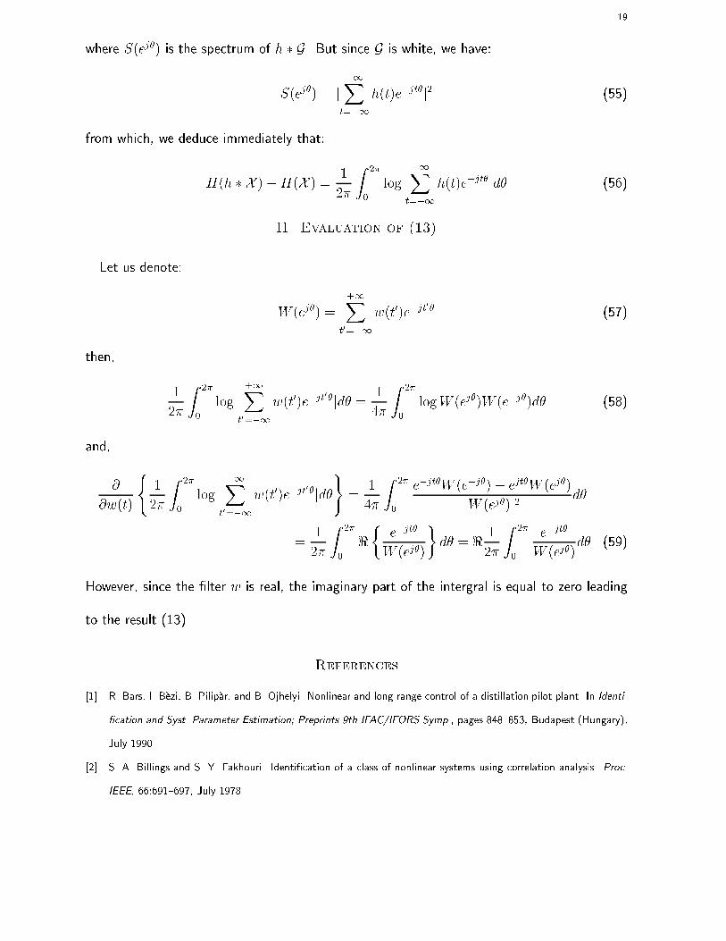
Quasi-nonparametric blind inversion of Wiener systems
24
Transcript of Quasi-nonparametric blind inversion of Wiener systems

1
Quasi-Nonparametric Blind Inversion of
Wiener Systems
Anisse Taleb (1,2), Jordi Sol�e (3), Christian Jutten (1,2)
(1) INPG-LIS, 46 Ave Flix Viallet, 38031 Grenbole Cedex, France
(2) GDR-PRC ISIS
(3) UNIVERSITAT DE VIC, c/ Sagrada fam��lia, 7 - 08500 Vic, Catalunya, Spain.
EDICS: 2SPTM 2NLIN 1MCHT 1NLHO
Correspondance author, email: [email protected]

2
Abstract
An e�cient procedure for the blind inversion of a nonlinear Wiener system is proposed. We proved that the
problem can be expressed as a problem of blind source separation in nonlinear mixtures, for which a solution
has been recently proposed. Based on a quasi-nonparametric relative gradient descent, the proposed algorithm
can perform e�ciently even in the presence of hard distortions.
I. Introduction
When linear models fail, nonlinear models, because of their better approximation capabilities,
appear to be powerfull tools for modeling practical situations. Examples of actual nonlinear
systems include digital satellite and microwave channels which are composed of a linear �lter
followed by a memoryless nonlinear travelling wave tube ampli�er [6], magnetic recording
channel, etc. Identi�cation of such systems is, therefore, of great theoretical and practical
interest.
Many researches have been done for the identi�cation and/or the inversion of such sys-
tems. Traditional nonlinear system identi�cation methods have been based on higher-order
input/output cross-correlations [2], or on the application of the Bussgang and Prices theorems
[3], [10] for nonlinear systems with Gaussian inputs.
These methods assume the availability of the nonlinear system input. However, in a real
world situation, one often does not have access to the system input: blind identi�cation of the
nonlinearity becomes then a necessary and a powerful tool. Although higher order statistics of
the output signal has been used in the detection of nonlinearities [11], [12] or in the identi�cation
of cascade of linear system - memoryless polynomial nonlinearity - linear system [13], blind
identi�cation of nonlinear systems has remained an intractable problem, except for a very
restricted class of inputs, mainly Gaussian.

3
It is well known that, unlike the case of linear systems, prior knowledge of the model is
necessary for nonlinear system identi�cation [14]. This paper is concerned by a particular
class of nonlinear systems. These are composed by a linear time invariant subsystem (�lter h)
followed by a memoryless nonlinear distortion (function f) (Figure 1). This class of nonlinear
systems, also known as Wiener systems, is not only another nice and mathematically attracting
model, but also a model found in various areas, such as biology: study of the visual system [5],
relation between the muscle length and tension [8], industry: description of a distillation plant
[1], sociology and psychology. See also [9] and the references therein. Despite its interest, at
our knowledge, no blind procedure exists for the inversion of such systems.
The paper organizes as follows. In section II, the model, notations and assumptions are
detailed. The cost function, based on mutual information, is proposed in section III. Derivation
of the cost function optimization algorithm is exposed in section IV. In V, practical issues for
implementing the algorithm are adressed. Finally, section VI illustrates the good behavior of the
proposed algorithm in a hard situation, and its e�ciency by means of Monte-Carlo simulations.
II. Model and assumptions
We suppose that the input of the system, S = fs(t)g is an unknown non-Gaussian indepen-
dent and identically distributed (iid) process, and that both subsystems h; f are unknown and
invertible. We are concerned by the restitution of s(t) by only observing the system's output.
This implies the blind design of an inverse structure (Figure 2), this structure will be composed
of the same subsystems than the Wiener system, i.e. a linear �lter and a memoryless nonlin-
earity, but in the reverse order, i.e. a Hammerstein system. The nonlinear part g is concerned
by the compensation of the distortion f without access to its input, while the linear part w is

4
a deconvolution �lter.
The following notation will be adopted through the paper. For each process Z = fz(t)g, z
denotes a vector of in�nite dimension, whose t-th entry is z(t). Following this notation, the
unknown input-output transfert can be written as:
e = f(Hs) (1)
where:
H =
0BBBBBBBBB@
� � � � � � � � � � � � � � �
� � � h(t + 1) h(t) h(t� 1) � � �
� � � h(t + 2) h(t + 1) h(t) � � �
� � � � � � � � � � � � � � �
1CCCCCCCCCA
(2)
denotes a square Toeplitz matrix of in�nite dimension and represents the action of the �lter h
on s(t). This matrix is nonsingular provided that the �lter h is invertible, i.e. h�1 exists and
satis�es h�1 � h = h � h�1 = �0, where �0 is the Dirac impulse at t = 0.
One can recognise in equation (1) the postnonlinear (pnl) model [15]. However, this model
has been studied only in the �nite dimentional case, in which it has been shown that, under
mild conditions, the system is separable provided that the input s has independent components,
and that the matrix H has at least two nonzero entries per row or per column.
Here, we conjecture that this will remain true for the in�nite dimension case. The �rst
separability condition is full�led since s has independent components due to the iid assumption.
Moreover, due to the particular structure of the matrixH, the second condition of separability
will always hold except if h is proportional to a pure delay.
5
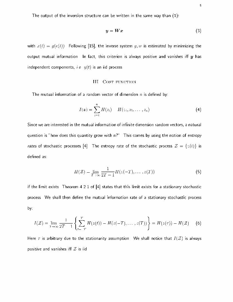
The output of the inversion structure can be written in the same way than (1):
y =Wx (3)
with x(t) = g(e(t)). Following [15], the inverse system g; w is estimated by minimizing the
output mutual information. In fact, this criterion is always positive and vanishes i� y has
independent components, i.e. y(t) is an iid process.
III. Cost function
The mutual information of a random vector of dimension n is de�ned by:
I(z) =nXi=1
H(zi)�H(z1; z2; : : : ; zn) (4)
Since we are interested in the mutual information of in�nite dimension random vectors, a natural
question is "how does this quantity grow with n?". This comes by using the notion of entropy
rates of stochastic processes [4]. The entropy rate of the stochastic process Z = fz(t)g is
de�ned as:
H(Z) = limT!1
1
2T + 1H(z(�T ); : : : ; z(T )) (5)
if the limit exists. Theorem 4.2.1 of [4] states that this limit exists for a stationary stochastic
process. We shall then de�ne the mutual information rate of a stationary stochastic process
by:
I(Z) = limT!1
1
2T + 1
(TX
t=�T
H(z(t))�H(z(�T ); : : : ; z(T )))
= H(z(�))�H(Z) (6)
Here � is arbitrary due to the stationarity assumption. We shall notice that I(Z) is always
positive and vanishes i� Z is iid.

6
Now, since S is stationary, and since h and w are time-invariant �lters, then Y is also
stationary, and I(Y) is de�ned by:
I(Y) = H(y(�))�H(Y) (7)
We need the following lemma, proof of which is given in Appendix A:
Lemma 1: Let X be a stationary stochastic process, and let h be an invertible linear time
invariant �lter, then:
H(h � X ) = H(X ) + 1
2�
Z 2�
0
logj+1Xt=�1
h(t)e�jt�jd� (8)
2
Since y(t) = h � x(t), one can write, applying lemma 1:
H(Y) = H(X ) + 1
2�
Z 2�
0
logj+1Xt=�1
w(t)e�jt�jd� (9)
Moreover, since x(t) = g(e(t)) and by using the stationarity of E = e(t), one can write:
H(X ) = limT!1
1
2T + 1
(H(e(�T ); : : : ; e(T )) +
TXt=�T
E [log g0(e(t))]
)
= H(E) + E [log g0(e(�))] (10)
Combining (9) and (10) in (7) leads �nally to:
I(Y) = H(y(�))� 1
2�
Z 2�
0
logj+1Xt=�1
w(t)e�jt�jd� � E [log g0(e(�))]�H(E) (11)
IV. Theoretical derivation of the inversion algorithm
To derive the optimization algorithm we need the derivatives of I(Y) (11) with respect to
the linear part w and with respect to the nonlinear function g.

7
A. Linear subsystem
For the linear subsystem w, this is quite easy since the �lter w is well parameterized by its
coe�cients. For the coe�cient w(t), corresponding to the t-th lag, we have:
@H(y(�))
@w(t)= �E[
@y(�)
@w(t) y(�)(y(�))] = �E[x(� � t) y(�)(y(�))] (12)
where y(�)(u) = (log py(�))0(u). Since, by stationarity, y(�) is independent of � , in the
following it will be denoted simply y. The second term of interest is (see appendix B):
@
@w(t)
(1
2�
Z 2�
0
logj+1X
t0=�1
w(t0)e�jt0�jd�
)=
1
2�
Z 2�
0
e�jt�P+1t=�1w(t)e
�jt�d� (13)
One recognises the f�tg-th coe�cient of the inverse of the �lter w, which we denote w(�t).
The derivatives of the other terms with respect to the w coe�cients are null, which leads, by
combining (12) and (13), to:
@I(Y)@w(t)
= �E[x(� � t) y(y(�))]� w(�t) (14)
Equation (14) is the gradient of I(Y) with respect to w(t). Considering a small relative
variation of w, expressed as the convolution of w by a "small" �lter �:
w! w + � � w (15)
the �rst order variation of I(Y) writes as :
�I(Y) = ��( y; y(y) + �) � � (0) (16)
where y; y(y)(t) = E[y(� � t) y(y(�))] and � is the identity �lter. One immediately notices
that taking:
� = �� y; y(y) + �
; (17)
8
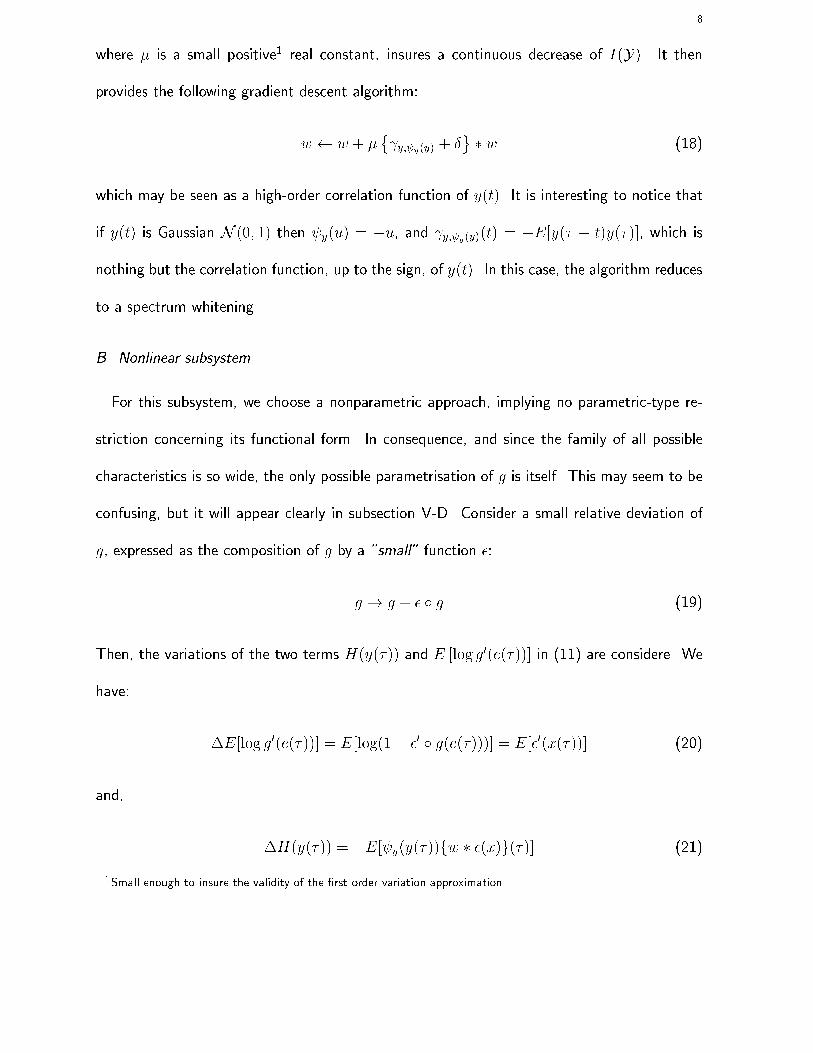
where � is a small positive1 real constant, insures a continuous decrease of I(Y). It then
provides the following gradient descent algorithm:
w w + �� y; y(y) + �
� w (18)
which may be seen as a high-order correlation function of y(t). It is interesting to notice that
if y(t) is Gaussian N (0; 1) then y(u) = �u, and y; y(y)(t) = �E[y(� � t)y(�)], which is
nothing but the correlation function, up to the sign, of y(t). In this case, the algorithm reduces
to a spectrum whitening.
B. Nonlinear subsystem
For this subsystem, we choose a nonparametric approach, implying no parametric-type re-
striction concerning its functional form. In consequence, and since the family of all possible
characteristics is so wide, the only possible parametrisation of g is itself. This may seem to be
confusing, but it will appear clearly in subsection V-D. Consider a small relative deviation of
g, expressed as the composition of g by a "small" function �:
g ! g + � � g (19)
Then, the variations of the two terms H(y(�)) and E [log g0(e(�))] in (11) are considere. We
have:
�E[log g0(e(�))] = E[log(1 + �0 � g(e(�)))] = E[�0(x(�))] (20)
and,
�H(y(�)) = �E[ y(y(�))fw � �(x)g(�)] (21)
1Small enough to insure the validity of the �rst order variation approximation.

9
It leads to a variation:
�I(Y) = �E[ y(y(�))fw � �(x)g(�)] � E[�0(x(�))] (22)
of I(Y). Now let us write:
�0(x) =
ZR
�(v)�0(x� v)dv (23)
�(x) =
ZR
�(v)�(x� v)dv (24)
then:
�I(Y) = �ZR
E[ y(y(�))fw � �(x� v)g(�) + �0(x(�)� v)]| {z }J(v)
�(v)dv (25)
To make a gradient descent, we may take:
�(v) = �Q � J(v) (26)
where � is a small positive real constant, and Q is any function such that:
ZR
J(v)Q � J(v)dv � 0; (27)
to insure that I(Y) decreases. Using the Parseval equality, the last condition becomes
ZR
jJ (�)j2<fQ(�)gd� � 0 (28)
where J and Q are the Fourier transforms of J and Q respectively and < denotes the real part.
It is thus su�cient to take <fQ(�)g > 0 for insuring the descent condition. The algorithm
writes then as:
g g + � fQ � Jg � g (29)

10
V. Practical issues
It is clear that (18) and (29) are unusable in practice. This section is concerned by
adapting these algorithms to an actual situation. We consider then a �nite discrete sam-
ple E = fe(1); e(2); : : : ; e(T )g. We assume that we already have computed the output of the
inversion system, i.e. X = fx(1); x(2); : : : ; x(T )g and Y = fy(1); y(2); : : : ; y(T )g. The �rst
question of interest is the estimation of the quantities involved in equations (18) and (29).
A. Estimation of y
Two approaches can be used to estimate y. The �rst approach consists in estimating the
pdf of y, and by y = (log py)0 one gets an estimate of y. A possible choice of an estimator
of py consists in using nonparametric approaches, in particular methods based on kernels [7].
Kernel density estimators are easy to implement and have a very exible form. However, they
su�er from the di�culty of the choice of the kernel bandwidth B. In fact, this choice strongly
depends on the criterion used to evaluate the performance of the estimation.
Formally, using normalized kernels2, one estimates py by:
py(u) =1
BT
TXt=1
K
�u� y(t)
B
�(30)
and y by:
y(u) =
PTt=1K
0
�u�y(t)B
�BPT
t=1K
�u�y(t)B
� (31)
In our experiments we used the Gaussian kernel (K has a Gaussian shape), however many other
kernel shapes can be good candidates (see [7] for more details). A "quick and dirty" method
2RRK(u)du = 1.

11
for the choice of the bandwith consists in using the rule of thumb h = 1:06 �y T�1=5 which
is based on the minimum asymptotic mean integrated error criterion. Probably better choices
could be used, but experimentally we noticed that the proposed estimator works �ne.
A second approach for the estimation of y is based on the direct mean square minimisation
of:
�( y) = E[( y(y)� y(y))2] (32)
which can be done without knowing the true function y. In fact, using:
E[ y(y) y(y)] = �E[ 0y(y)]
equation (32) reduces to:
�( y) = E[ y(y)2 + 2 0y(y)] + E[ y(y)
2] (33)
in which the true function y appear as a constant term. y being nonlinear, it could then
be modeled, for example, by a neural network [16] and trained using the backpropagation
algorithm. This approach has not been used in this paper where we prefer a nonparametric
approach.
B. Estimation of y; y(y)
According to the previous subsection, it is assumed that one has an estimator of y. We are
now interested in estimating:
y; y(y)(t) = E[y(� � t) y(y(�))] (34)
Assuming y(t) is ergodic, one can get the estimate:
y; y(y)(t) =1
T
TX�=1
y(� � t) y(y(�)) (35)

12
where, by convention, y(�) = 0 for � < 1 and � > T . This estimate corresponds to the use of
a rectangular window. Other estimates can be obtained by choosing di�erent windows. Since,
in theory, y; y(y)(0) = �1, y; y(y)(0) will be set to �1 without computing. Equation (35) is
a convolution, it implementation is done by resort to the FFT which reduces dramatically the
computation load.
C. Filter estimation
In pratical situations, the �lter w, updated according to:
w w + �f y; y(y) + �g � w; (36)
has a �nite length (FIR). The result of the convolution of w with y; y(y)+� should be truncated
to �t the size of w. A smooth truncation, e.g. using of a Hamming window, is preferable to
avoid overshooting.
D. Nonlinear subsystem estimation
We recall that no parametrisation of g is used. Then, one would ask the intriguing question
"How would I compute the output of the nonlinear subsystem without having g?". In fact,
applying the equation (29) to the t-th element of the sample E , and using x(t) = g(e(t)), one
gets:
x(t) x(t) + � fQ � Jg (x(t)) (37)
As (37) converges, for each input sample e(t), we know that x(t) = g(e(t)). A simple nonlinear
approximation using the samples [x(t); e(t)]; t = 1; : : : ; T could lead to an approximation of
teh function g. However, this is not necessary and (37) has the advantage to be nonparametric,
and e�cient for any g.

13
E. Estimation of Q � J
This function is necessary to adapt the output of the nonlinear subsystem, and can be
estimated by:
Q � J(v) = 1
T
TXt=1
�Q0(v � x(t)) + y(y(t))fw �Q(v � x)g(t) (38)
A possible choice of Q is:
Q(u) =
8>><>>:�u if u � 0
0 otherwise
(39)
which is very simple from a computational point of view. The real part of its Fourier transform
is <Q(!) = 1=!2 and satis�es (28).
In order to reduce the computational load when T is large, equation (38) can be simpli�ed.
Instead of computing Q�J at each sample x(t), it is computed only at N � T equally-spaced
points in the range [xmin; xmax] of the input signal x(t). The values of Q�J at the sample x(t)
are then obtained by linear interpolation. Equation (37) is in fact quite robust to sampling:
this can be explained by the low-pass �ltering e�ect of Q on J .
F. Indeterminacies
The output of the nonlinear subsystem x(t); t = 1; : : : ; T should be centered and normalized.
In fact, the inverse of the nonlinear distortion can be restored only up to a scale and a shift
factor. For the linear subsystem, the output y(t); t = 1; : : : ; T should also be normalized due

14
to scale indeterminacy on w. For example, the mean and variance of x(t) are estimated by:
mx =1
T
TXt=1
x(t) (40)
�x =
vuut 1
T
TXt=1
(x(t)� mx)2 (41)
and x(t) is normalized by:
x(t) x(t)� mx
�x(42)
One can use the same normalisation scheme for y(t).
VI. Experimental results
A. Hard experiment
To test the previous algorithm, we simulate a hard situation. The iid input sequence s(t),
shown in �gure 5, is generated by applying a cubic distortion to an iid Gaussian sequence. The
�lter h is FIR, with the coe�cients:
h = [0:826;�0:165; 0:851; 0:163; 0:810]
Its frequency response is shown in �gure 3. Figure 4 shows that h has two zeros outside the
unit circle, which indicates that h is non-minimum phase.
The nonlinear distortion is a hard saturation f(u) = tanh(10u). The observed sequence is
shown in �gure 5.
The algorithm was provided with a sample of size T = 1000. The size of the impulse response
of w was set to 51 with equal size for the causal and anti-causal parts. Estimation results,
shown in �gures 5,6 and 7, prove the good behavior of the proposed algorithm. The phase of

15
w (Figure 6) is composed of a linear part which corresponds to an arbitrary uncontrolled but
constant delay, and of a nonlinear part which cancels the h phase.
B. Performance analysis
The performance of the proposed algorithm is evaluated by means of Monte-Carlo simula-
tions. Since we are interested in restoring the original sequence, a good performance index
consists in evaluating the error between the original signal s(t) and the restored signal y(t).
The performance index writes then as:
PT = E
"1
T
TXt=1
(y(t)� s(t))2#
(43)
in which, it is supposed that y(t) has been properly delayed and rescaled.
A uniformally distributed signal in the range [�p3;p3] is chosen for the simulations. Filter
h is a simple low-pass �lter with coe�cients [1; 0:5], and the nonlinear distortion is still f(u) =
tanh(10u). Figure 8 shows the results of the simulations, where each point is the average of
50 experiments. As one can expect, the performance index decreases when the sample size T
increases.
C. Real data
The previous procedure has been tested on real data. Figure 9 shows a seismic refraction
pro�le recorded using a vessel and an Ocean Bottom Seismometer (OBS) over the Beaulieu
plateau in France.
Each wave correspond to the signal recorded by the unique sensor, located on the sea bottom
(OBS), in response to the shots which are produced at regular time intervals by the vessel which
moves at constant speed.

16
In this experiment, the proposed procedure provides an estimate of the nonlinearity g which
is far from a linear characteristic. The output of the nonlinear processing is shown in Figure
10.
Figure 11 compares a purely linear deconvolution and the proposed nonlinear method as-
suming the existence of a nonlinear memoryless distortion. We can notice that the proposed
procedure provides an enhanced version of the purely linear deconvolution revealing hidden
structures not emphasized by the linear deconvolution. However, these results are currently
not well understood since seismic experts consider usually purely linear models. The only
thing that can be said is that the linear model does not hold since our procedure revealed the
existence of a nonlinearity.
VII. Final remarks and conclusion
In this paper a blind procedure for the inversion of a nonlinear Wiener system was pro-
posed. Contrary to other blind identi�cation procedures, the system input is not assumed to
be Gaussian. Moreover, the nonlinear subsystem is unknown or not directly identi�able. The
inversion procedure is based on a quasi-nonparametric relative gradient descent of the mutual
information rate of the inversion system output. It is inspired from recent results on blind
source separation in nonlinear mixtures.
One may notice that some quantities involved in the algorithm can be e�ciently estimated
by resort to FFT and interpolation, which reduces dramatically the computational cost. The
estimation of g is done implicitely: only the values of x(t) = g(e(t)); t = 1; : : : ; T are esti-
mated. One can further use any regression algorithm based on these data to estimate g, e.g.
neural networks, splines, etc.
17
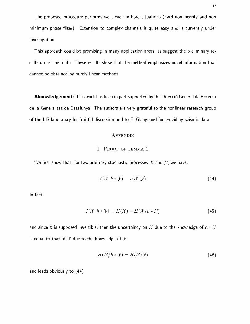
The proposed procedure performs well, even in hard situations (hard nonlinearity and non
minimum phase �lter). Extension to complex channels is quite easy and is currently under
investigation.
This approach could be promising in many application areas, as suggest the preliminary re-
sults on seismic data. These results show that the method emphasizes novel information that
cannot be obtained by purely linear methods.
Aknowledgement: This work has been in part supported by the Direcci�o General de Recerca
de la Generalitat de Catalunya. The authors are very grateful to the nonlinear research group
of the LIS laboratory for fruitful discussion and to F. Glangeaud for providing seismic data.
Appendix
I. Proof of lemma 1
We �rst show that, for two arbitrary stochastic processes X and Y, we have:
I(X ; h � Y) = I(X ;Y) (44)
In fact:
I(X ; h � Y) = H(X )�H(X =h � Y) (45)
and since h is supposed invertible, then the uncertaincy on X due to the knowledge of h � Y
is equal to that of X due to the knowledge of Y:
H(X =h � Y) = H(X =Y) (46)
and leads obviously to (44).
18
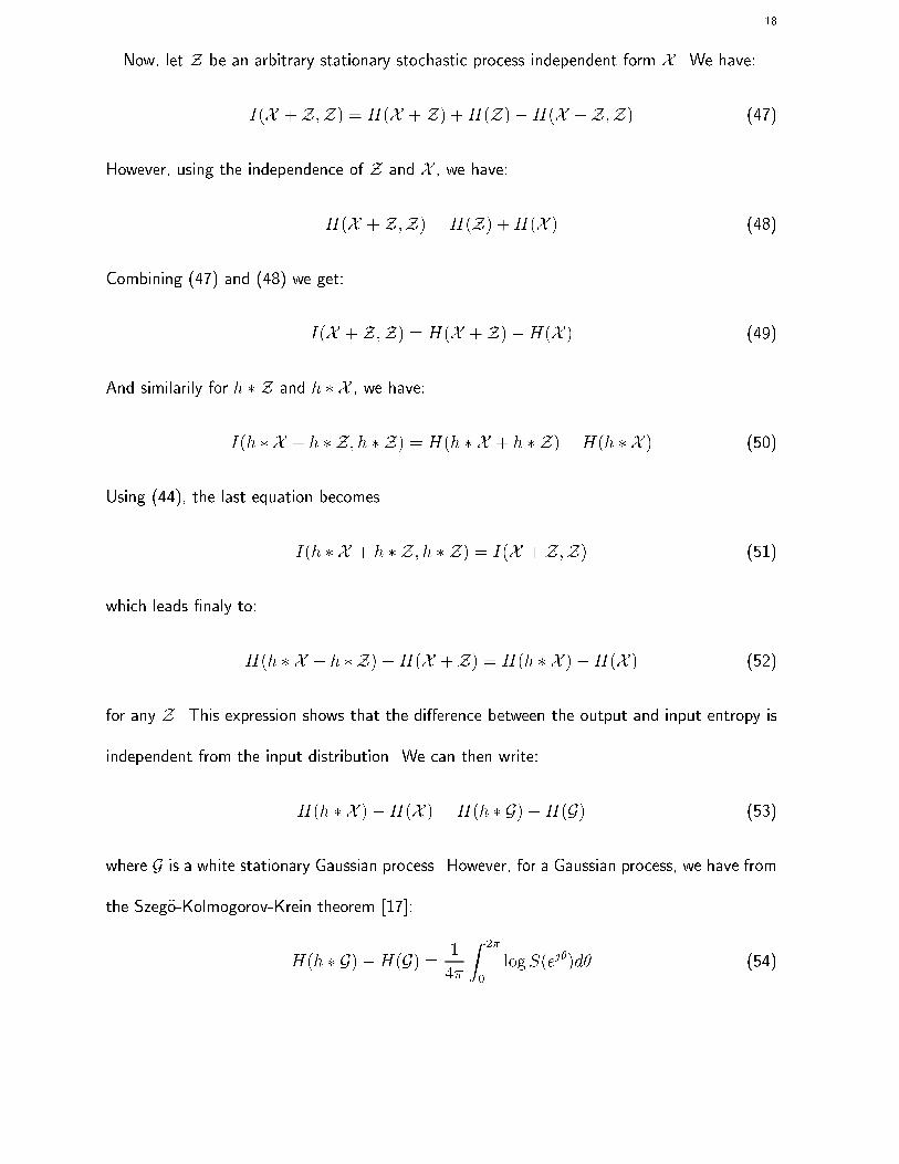
Now, let Z be an arbitrary stationary stochastic process independent form X . We have:
I(X + Z;Z) = H(X + Z) +H(Z)�H(X + Z;Z) (47)
However, using the independence of Z and X , we have:
H(X + Z;Z) = H(Z) +H(X ) (48)
Combining (47) and (48) we get:
I(X + Z;Z) = H(X + Z)�H(X ) (49)
And similarily for h � Z and h � X , we have:
I(h � X + h � Z; h � Z) = H(h � X + h � Z)�H(h � X ) (50)
Using (44), the last equation becomes
I(h � X + h � Z; h � Z) = I(X + Z;Z) (51)
which leads �naly to:
H(h � X + h � Z)�H(X + Z) = H(h � X )�H(X ) (52)
for any Z. This expression shows that the di�erence between the output and input entropy is
independent from the input distribution. We can then write:
H(h � X )�H(X ) = H(h � G)�H(G) (53)
where G is a white stationary Gaussian process. However, for a Gaussian process, we have from
the Szeg�o-Kolmogorov-Krein theorem [17]:
H(h � G)�H(G) = 1
4�
Z 2�
0
logS(ej�)d� (54)
19
where S(ej�) is the spectrum of h � G. But since G is white, we have:
S(ej�) = j+1Xt=�1
h(t)e�jt�j2 (55)
from which, we deduce immediately that:
H(h � X )�H(X ) = 1
2�
Z 2�
0
logj+1Xt=�1
h(t)e�jt�jd� (56)
II. Evaluation of (13)
Let us denote:
W (ej�) =+1X
t0=�1
w(t0)e�jt0� (57)
then,
1
2�
Z 2�
0
logj+1X
t0=�1
w(t0)e�jt0�jd� = 1
4�
Z 2�
0
logW (ej�)W (e�j�)d� (58)
and,
@
@w(t)
(1
2�
Z 2�
0
logj+1X
t0=�1
w(t0)e�jt0�jd�
)=
1
4�
Z 2�
0
e�jt�W (e�j�) + ejt�W (ej�)
jW (ej�)j2 d�
=1
2�
Z 2�
0
<�
e�jt�
W (ej�)
�d� = < 1
2�
Z 2�
0
e�jt�
W (ej�)d� (59)
However, since the �lter w is real, the imaginary part of the intergral is equal to zero leading
to the result (13).
References
[1] R. Bars, I. B�ezi, B. Pilip�ar, and B. Ojhelyi. Nonlinear and long range control of a distillation pilot plant. In Identi-
�cation and Syst. Parameter Estimation; Preprints 9th IFAC/IFORS Symp., pages 848{853, Budapest (Hungary),
July 1990.
[2] S. A. Billings and S. Y. Fakhouri. Identi�cation of a class of nonlinear systems using correlation analysis. Proc.
IEEE, 66:691{697, July 1978.

20
[3] E. D. Boer. Cross-correlation function of a bandpass nonlinear network. Proc. IEEE, 64:1443{1444, September
1976.
[4] T. M. Cover and J. A. Thomas. Elements of Information Theory. Wiley Series in Telecommunications, 1991.
[5] A. C. den Brinker. A comparison of results from parameter estimations of impulse responses of the transient visual
system. Biol. Cybern., 61:139{151, 1989.
[6] K. Feher. Digital Communications{Satellite/Earth Station Engineering. Englewood Cli�s, NJ: Prentice-Hall, 1993.
[7] W. H�ardle. Smoothing Techniques, with implementation in S. Springer-Verlag, 1990.
[8] I. W. Hunter. Frog muscle �ber dynamic sti�ness determined using nonlinear system identi�cation techniques.
Biophys. J., 49:81a, 1985.
[9] I. W. Hunter and M. J. Korenberg. The identi�cation of nonlinear biological systems: Wiener and Hamerstein
cascade models. Biol. Cybern., 55:135{144, 1985.
[10] G. Jacovitti, A. Neri, and R. Cusani. Methods for estimating the autocorrelation function of complex stationary
processes. IEEE Trans. ASSP., 35:1126{1138, August 1987.
[11] C. L. Nikias and Petropulu A. P. Higher-Order Spectra Analysis - A Nonlinear Signal Processing Framework.
Englewood Cli�s, NJ: Prentice-Hall, 1993.
[12] C. L. Nikias and M. R. Raghuveer. Bispectrum estimation: A digital signal processing framework. Proc. IEEE,
75:869{890, July 1987.
[13] S. Prakriya and D. Hatzinakos. Blind identi�cation of LTI-ZMNL-LTI nonlinear channel models. Biol. Cybern.,
55:135{144, 1985.
[14] M. Schetzen. Nonlinear system modeling based on the Wiener theory. Proc. IEEE, 69:1557{1573, December 1981.
[15] A. Taleb and C. Jutten. Source separation in postnonlinear mixtures. IEEE trans. S.P.- To appear.
[16] A. Taleb and C. Jutten. Entropy optimization, application to blind source separation. In ICANN 97, pages 529{534,
Lausanne (Switzerland), October 1997.
[17] P. Whittle. Some recent contributions to the theory of stationary processes. Almquist and Wiksell, 1954. Appendix
2 in H. Wold, A study in the analysis of stationary time series.

21
h
f
s(t) e(t)
Fig. 1. Wiener system.
w
g
e(t) x(t) y(t)
Fig. 2. Wiener system inversion structure - Hammerstein system.
0 0.1 0.2 0.3 0.4 0.5 0.6 0.7 0.8 0.9 1−400
−300
−200
−100
0
Normalized frequency (Nyquist == 1)
Pha
se (
degr
ees)
0 0.1 0.2 0.3 0.4 0.5 0.6 0.7 0.8 0.9 1−15
−10
−5
0
5
10
Normalized frequency (Nyquist == 1)
Mag
nitu
de R
espo
nse
(dB
)
Fig. 3. h frequency domain response.

22
−1 −0.5 0 0.5 1
−1
−0.5
0
0.5
1
Real part
Imag
inar
y pa
rt
Fig. 4. Zeros of h.
0 100 200 300 400 500 600 700 800 900 1000−1
−0.8
−0.6
−0.4
−0.2
0
0.2
0.4
0.6
0.8
1
0 100 200 300 400 500 600 700 800 900 1000−1
−0.8
−0.6
−0.4
−0.2
0
0.2
0.4
0.6
0.8
1
0 100 200 300 400 500 600 700 800 900 1000−8
−6
−4
−2
0
2
4
6
8
Fig. 5. From left to right: Original input sequence s(t), Observed sequence e(t), Restored sequence y(t).
0 0.1 0.2 0.3 0.4 0.5 0.6 0.7 0.8 0.9 1−5000
−4000
−3000
−2000
−1000
0
Normalized frequency (Nyquist == 1)
Pha
se (
degr
ees)
0 0.1 0.2 0.3 0.4 0.5 0.6 0.7 0.8 0.9 1−10
−5
0
5
10
15
Normalized frequency (Nyquist == 1)
Mag
nitu
de R
espo
nse
(dB
)
Fig. 6. Estimated inverse of h: w frequency domain response.

23
−1 −0.8 −0.6 −0.4 −0.2 0 0.2 0.4 0.6 0.8 1−4
−3
−2
−1
0
1
2
3
4
Fig. 7. Estimated inverse of the nonlinear characteristic f : x(t) vs. e(t)
200 300 400 500 600 700 800 900 1000−18
−16
−14
−12
−10
−8
−6
−4
T
Per
form
ance
inde
x (d
B)
Fig. 8. Performance index versus sample size T .

24
50 100 150 200 250
−3
−2
−1
0
1
2
3
x 105
Fig. 9. Original seismic data
50 100 150 200 250
−1.5
−1
−0.5
0
0.5
1
1.5
x 105
Fig. 10. Output of the nonlinear processing stage
50 100 150 200 250
−150
−100
−50
0
50
100
150
50 100 150 200 250
−150
−100
−50
0
50
100
150
Fig. 11. Linear deconvolution vs. Nonlinear Wiener system deconvolution