The tax benefit of income smoothing

Electronic copy available at: http://ssrn.com/abstract=1836577

The Tax Benefit of Income Smoothing

Kristian Rydqvist Steven T. Schwartz Joshua D. Spizman∗

November 2011

Abstract

There is a long-held belief that a worker can reduce tax liability by contributing to aprivate pension plan when marginal tax rates are high and withdraw pension benefitswhen marginal tax rates are low. We quantify the tax benefit of income smoothingthrough the private retirement system and find that it is small. This conclusion is ofconsiderable importance to investment advisers, tax policymakers, and scholars engagedin financial retirement planning.

Keywords: private pensions, life-cycle model, tax progressivity.JEL Classification Numbers: G11, G18, G23, H24, D91.

∗We thank participants at Binghamton University, Financial Management Association, Syracuse University, theSouthern Finance Association, and our discussants Steven Beach and Raphael Kuznetsovski for comments and usefulsuggestions. Rydqvist: Binghamton University and CEPR; e-mail: [email protected] . Schwartz: e-mail:[email protected] . Spizman: Loyola Marymount University; email: [email protected] .

Electronic copy available at: http://ssrn.com/abstract=1836577

1 Introduction

Deferral of income taxes to retirement is a cornerstone of the U.S. private pension system. This

principle makes it possible to contribute to a private pension plan during work years when marginal

tax rates are relatively high and withdraw from the pension plan when marginal tax rates tend to

be low. A widely-held belief is that, as a result of the progressivity of the tax code, the tax benefit

of smoothing income between working years and old age is large, but little work has been done to

quantify how much taxes can be saved.1 Our objective is to quantify the tax benefit of income

smoothing. Ascertaining the value of the smoothing benefit should be of interest to scholars engaged

in research on savings and consumption decisions and on the growth of financial intermediation,

investment advisors and union leaders designing retirement plans, and policymakers interested in

how tax incentives affect savings decisions.

Ippolito (1986) conducts an extensive analysis of the United States private pension system and

estimates the potential smoothing benefit as 20% of life-time taxes or, expressed in terms of tax

rates, a reduction of the effective tax rate by five to six percentage points. His calculations are based

on a life-cycle consumption model and actual taxes paid from the IRS Statistics of Income. Some

other attempts such as those by Ozanne and Lindeman (1987) and Horan (2005) are only suggestive

because the tax rates at contribution and withdrawal are treated as exogenous. For example,

Ozanne and Lindeman (1987) assume that the contribution rate is 28% and the withdrawal rate

15%, thus implying that tax liability is almost cut in half. Gokhale, Kotlikoff, and Neumann (2008)

use a life-cycle financial planner program (Economic Security Planner) to numerically evaluate the

tax benefits of saving before tax. However, in their analysis, the smoothing benefit is mixed in

with other effects, notably that investment income remains untaxed until withdrawal of funds in

retirement.

In this paper, we update and extensively develop the work of Ippolito (1986). Relative to

the attention paid to the smoothing benefit in textbooks, articles, by investment advisers, and by

Ippolito (1986), our estimate is surprisingly small. Under extreme behavioral assumptions that1E.g., Ippolito (1986), Feenberg and Skinner (1989), Ragan (1994), Burmann, Gale, and Weiner (2001), Turner

(2005), Lankford (2008), Horan (2009), and Nishiyama (2010). See also the tax treatment of pensions in the Ency-clopedia of Taxation and Tax Policy.

1

entail lifetime planning from the time the worker enters the job market until death, the average

worker cannot reduce the effective tax rate by more than 3.2 percentage points. The main reason is

that the United States income tax system is not sufficiently progressive. If we add Social Security,

the tax rate reduction resulting from lifetime income smoothing decreases to 1.7 percentage points.

We believe that such a small magnitude is unlikely to motivate the type of disciplined savings

necessary to obtain the smoothing benefit.

As an example of the potential smoothing benefit, consider a worker with annual taxable income

$300,000.2 Using the 2010 federal income tax table, the standard deduction, and two exemptions,

the effective tax rate on this income is 23.3%. If the worker could split his income equally between

work years and retirement years, the taxable income would decrease to $150,000 and the effective tax

rate drop to 16.4%. Accordingly, the smoothing benefit equals the 6.9 percentage point reduction

in the effective tax rate. This is a considerable tax benefit worth paying attention to, but many

real-world features reduce it. (i) Time spent in the work force tends to exceed the number of

retirement years. (ii) Social Security income replaces private retirement income. (iii) Contribution

limits and borrowing restrictions induce the worker to deviate from the tax-minimizing solution to

support other consumption and saving goals. We illustrate how some of these real-world features

bring down the smoothing benefit from 6.9% in the example to as little as 1.7%, on average.

Our findings on the magnitude of the smoothing benefit are robust to a variety of parameter

choices. We perform comparative statics on real interest, income growth (income variability),

uncertainty, life expectancy, the savings rate, and the years spent saving for retirement. Real

interest influences the smoothing benefit similar to Social Security: it fills up lower marginal tax

brackets in retirement with capital income and, thus, prevents the worker from using them for

smoothing labor income. Income growth and increased life expectancy raise the smoothing benefit;

income growth because it represents income variability, which can be beneficially smoothed, and

increased life expectancy because it increases the number of years available for smoothing. However,

the effects of both income growth and increased life expectancy as well as variations in the savings

rate and the start of retirement savings are all relatively small because of the lack of progressivity in2This example is inspired by and closely-related to the example of income shifting between spouses and children

provided by Stiglitz (1988a).

2

the United States personal income tax code. Somewhat surprisingly, uncertainty is largely irrelevant

to the smoothing benefit.

Historical smoothing benefit calculations from 1950 conclude our analysis. The historical time-

series sheds light on Ippolito’s hypothesis that the smoothing benefit is one of the reasons for the

growth of the private pension system in the United States. As the smoothing benefit is quite small

throughout most of the post-war period, the tax benefit of income smoothing does not appear to

be a significant factor in the growth of union led retirement plans. In defense of Ippolito (1986),

who studies the growth of the private pension system right before The Tax Reform Act of 1986

(TRA 1986), the smoothing benefit is briefly higher at this point than at any other point in time

and may have attracted the attention of union leaders and other retirement planners. In addition,

nothing in our paper rules out Ippolito’s other assertion that deferral of investment income tax has

played a major role in the creation of the private retirement system.3

The income smoothing problem in our paper adds to the literature on tax shifting within

a progressive system. There are papers studying the tax implications of shifting income across

spouses, unmarried couples, from parents to children, and across households.4 Also, the tax code

itself permits income smoothing. There are carry back and carry forward provisions for corporations

(operating losses) and households (capital losses). Farmers and fishermen can pay tax on income

averaged over the current year and the three past years and, during a twenty-year period before

TRA 1986, income averaging was available to the general tax payer.

The rest of the paper is organized as follows: Section 2 provides the reader with a short summary

of the main features of the private and public pension systems in the United States. In the next

Section 3, we derive the tax implications of income smoothing within a stylized tax table with only

three income brackets and large tax rate jumps. In Section 4, we apply the model to personal

income taxation in the United States 2010, and examine the robustness to parameters choices. The

section ends with the analysis of the historical United States time-series. Section 5 concludes the3See Rydqvist, Spizman, and Strebulaev (2010) for statistical test of this hypothesis in a cross-country and time-

series panel data set.4Stephens and Ward-Batts (2004) analyze spouses, Eissa and Hoynes (2000) study unmarried couples, and Stiglitz

(1988b) discusses shifting income from parents to children. Green and Rydqvist (1999) and Rydqvist (2011) examineinterpersonal netting of stock market gains and losses through trading in lottery bonds.

3

paper.

2 Institutional Background

In the United States, there is an array of retirement savings options. We describe the most relevant

options to our study. We classify options according to the tax provisions that attach to them. Other

important attributes include the sponsor, the party who bears the risk of investment performance,

and the option of not participating.

A large class of retirement savings options allows for pre-tax contributions to savings, tax-free

growth, and taxed withdrawals. Options in this class include 401(k), 403(b), 414(h), and 457(g)

employer-sponsored retirement savings plans. Qualifying contributions to traditional Individual

Retirement Accounts (IRAs) are also included. The difference between IRAs and the other options

is that IRAs are self-initiated, while 401(k) products must be provided by employers. Also, the

statutory limits on IRA contributions are relatively small. Defined benefit pension plans also belong

to this class. Although workers may not have to contribute explicitly to their pension plan it is often

the case that pension benefits are granted in lieu of wage increases (Lowenstein (2008)). Hence

defined benefit pension plans offer implicit pre-tax retirement savings. The important distinction

between defined contribution plans such as 401(k)s and defined benefit plans is the party that bears

the risk of investment performance. In the former it is the worker, in the latter it is the employer.

A second option for retirement savings is an after-tax contribution that offers tax free growth and

withdrawal of earnings. Options in this class are employer-sponsored Roth 401(k)s and self-initiated

Roth IRAs. As in the pre-tax case, the Roth 401(k) allows for significantly higher statutory limits

on contributions than the Roth IRA. It is also possible to convert traditional IRAs and 401(k)s to

Roth plans. Under a flat-tax system, Roth and traditional plans yield identical tax savings. The

Roth account also has the advantage of higher effective contribution limits (see Burmann, Gale,

and Weiner (2001)).

A third option, that is generally not of great importance, are after tax contributions that offer

tax free earnings growth but not tax free withdrawal. Most notable in this class are contributions to

traditional IRAs that do not qualify for pre-tax treatment. For individuals covered by a retirement

4

plan by their employers, the income limit excludes many individuals who would have the financial

resources for savings from qualifying for pre-tax treatment of contributions. For individuals without

an employer-sponsored plan there is no income limit, however there are significant limits on the size

of contributions relative to 401(k) plans. United States Savings Bonds have similar provisions in

that they are after-tax savings vehicles that accrue earnings tax free but are taxed upon withdrawal.

One difference between savings bonds and IRAs is that savings bond income is not taxable at the

state and local level.

By far the most important source of retirement income in the United States is Social Security.

Unlike all of the options described above, Social Security is mandatory for most workers in the

United States. Overall Social Security accounts for about 40% of retirees’ income and virtually

100% of income for the bottom third of retirees (Reno and Lavery (2007)). Social Security shares

some tax attributes with all three retirement savings options described above. Contributions from

workers are made after tax, there are no taxes paid during accumulation of benefits and, for many

retirees, benefits are not taxed upon withdrawal. In this sense, Social Security acts like a Roth IRA

or Roth 401(k). Beginning in 1984, individuals who have significant income in retirement other

than Social Security may have some of their Social Security benefits taxed as regular income. For

these individuals Social Security acts, in part, like non-qualified contributions to traditional IRAs.

Of particular note is that withdrawals from 401(k) plans and similar products are considered other

income while withdrawals from Roth products are not. Therefore, savings for retirement pre-tax

may come at a cost of increased taxes on Social Security benefits. Finally, half of Social Security

premiums are paid by employers. To the extent that these premiums substitute for taxable wages,

Social Security resembles a private pension and, hence, provides some smoothing benefits (Vroman

(1974) and Ippolito (1986)).

5

3 Income Smoothing

3.1 Zero Interest and No Income Growth

We analyze the consumption and savings decision of a worker who can save before income tax in

a retirement account that is either a company pension, a 401(k)-type account, or an Individual

Retirement Account (IRA). The worker contributes to the retirement account over n work years to

Figure 1: Life-Cycle Model

0

25

50

75

100

125

25 35 45 55 65 75

Perc

ent

Age

Save

Dis-save

The figure shows the annual before-tax income (solid line) and annual income smoothed over adult

life time (dotted line). We assume 40 work years and 16 retirement years.

support consumption over m − n retirement years. A numerical example is provided in Figure 1

assuming certainty, zero interest, and no income growth. The worker has an annual income of 100

during work years and zero income during retirement years, he begins working at age 25, he retires

at age 65, and he dies at age 81. In this example that entails perfect income smoothing over the

life cycle the before-tax savings rate is 28.6%.

We consider a worker who maximizes his after-tax income by solving a tax-minimization problem

and, then, uses the capital market to reach his desired life-time consumption path. The capital

market is represented by a Roth-style savings account that preserves all the tax benefits of the

regular retirement account except the smoothing benefit. Assuming a Roth account as opposed to

6

a regular savings account allows us to isolate the pure smoothing benefit from the other major tax

benefit of a retirement account, that income on the investment portfolio compounds at the before-

tax rate of return. The two savings accounts provide the worker with a choice between smoothing

income before tax in the regular account or after tax in the Roth account. We also assume that

the worker can save as much for retirement as he wants (no contribution limit), he can withdraw

funds from either account without penalty, and he can borrow any amount he wishes against future

income. These assumptions allow us to analyze the tax-minimization problem independently of the

utility-maximization problem.5 In what follows, we explicitly solve the tax-minimization problem

only, and we abstain from parameterizing the life-cycle consumption model. Our approach makes

the smoothing benefit the largest possible. Realistic modeling of life-cycle consumption behavior

with capital market restrictions on borrowing and lending would only reduce the smoothing benefit

relative to the tax-minimizing benchmark.

We analyze the tax-minimization problem assuming zero interest, no growth, and full certainty

over future income and tax liability. After we have presented the base case model, we extend

the analysis to include the effects of positive interest and income growth in Subsection 3.2, and

uncertainty in Subsection 3.3. Undoubtedly, real interest reduces the smoothing benefit and income

growth raises it. In our calibrations of the model to the United States tax code in Section 4, we

take an agnostic view and assume that the two effects approximately cancel out. Then, we show

that uncertainty is irrelevant to the smoothing benefit. Hence, while we believe that uncertainty

is a first-order determinant of life-cycle consumption behavior, we find that uncertainty does not

matter to the tax-minimization problem.

3.1.1 Tax-Minimization Problem

The worker’s objective is to choose the before-tax savings rate φ that minimizes lifetime tax liability:

minφ

T = nT ((1− φ)Y ) + (m− n)T(

nφY

m− n

), (1)

5The corresponding assumption that allows the researcher to separate the tax problem from the investment problemis used by Constantinides (1983), Huang (2008), and others.

7

where Y is annual income, T (·) is the tax liability function, n is the number of work years, and

m− n is the number of retirement years. The first term on the right hand side is the tax liability

on work income, and the second term is the tax liability on retirement income. The first-order

condition for a minimum requires that the marginal tax rate during work years and retirement

years are equal:

T ′((1− φ)Y ) = T ′(

nφY

m− n

). (2)

One specific solution that we refer to as perfect income smoothing is when work year income equals

retirement year income:

φ =m− n

m. (3)

Generally, the tax-minimization problem has multiple solutions because the tax liability function is

piecewise linear. As long as marginal tax rates are different during work years and retirement years,

tax liability can be reduced by shifting income, but when marginal tax rates are equal, shifting

income between work years and retirement years does not change tax liability.

Figure 2: Stylized Tax Table

0

10

20

30

40

50

60

0 10 20 30 40 50 60 70 80 90 100

Mar

gina

l tax

rate

(%)

Taxable income (000s)

This figure plots marginal and effective tax rates for a stylized tax table with three income brackets

and marginal tax rates at 0%, 20%, and 50%. The break points between income brackets are $10,000

and $50,000, respectively.

8

We numerically illustrate the properties of the solution to the tax-minimization problem using a

stylized tax table. Later, in Section 4, we quantify the smoothing benefit using United States 2010

tax tables. The stylized tax table in Figure 2 is a step function with three income brackets and

marginal tax rates at 0%, 20%, and 50%. The breakpoints between income brackets are $10,000

and $50,000, respectively. Within each income bracket the marginal tax rate is constant. The

effective tax rate curve plotted below (dotted line) is an increasing function with kinks at the break

points between income brackets. The stylized tax table has few income brackets as is typical after

TRA 1986, but the tax rate increments between income brackets have been exaggerated to bring

out the model properties.6

Figure 3: Tax-Minimizing Savings Rate

0

25

50

75

100

0 10 20 30 40 50 60 70 80 90 100

Pre-

tax

savi

ngs

rate

(%)


The figure shows the tax-minimizing savings rate with perfect smoothing φ = (m − n)/m (solid

middle line), the maximum φmax (solid line above), and the minimum φmin (dotted line below)

using the stylized tax table, 40 work years, and 16 retirement years.

The range of solutions within the stylized tax table can be seen in Figure 3. The solid line

above displays the maximum solution φmax and the dotted line below the minimum solution φmin.

The horizontal line in the middle represents the special case when income is perfectly smoothed

over the life cycle. Perfect smoothing is the unique solution to the tax-minimization problem where6Tax tables before TRA 1986 often have more than 30 income brackets. Such tax tables would be better approx-

imated by a continuous function. Interestingly, such tax tables exist in Germany, where the marginal tax rate isdetermined by a polynomial.

9

the φmax and φmin functions intersect near each breakpoint Yb:

Y = Yb ×(

m

n

). (4)

At this income level, tax liability is minimized by shifting all income out of the higher income

bracket into the lower brackets. At income levels below $625, any savings rate φ ∈ [0%, 100%]

is a tax-minimizing solution as the worker can shift his entire income in or out of the retirement

account without ever being liable for income tax.

3.1.2 Smoothing Benefit Measure

To measure the tax benefit of income smoothing, we define lifetime tax-liability with and without

income smoothing:

Non-Smooth = nT (Y ).

Smooth = nT ((1− φ)Y ) + (m− n)T(

nφYm−n

).

(5)

The difference between these terms divided by lifetime income is a natural measure of the tax

benefit of income smoothing:

SMOOTH =Non-Smooth− Smooth

nY. (6)

In the special case of perfect income smoothing, we have φ = (m−n)/m, and the smoothing benefit

can be expressed as a reduction of the effective tax rate τ(·) in the amount:

SMOOTH = τ(Y )− τ

(nY

m

). (7)

The smoothing benefit measure increases with the slope of the effective tax rate curve, which

depends on tax progressivity.7 The effective tax rate curve is upward-sloping when the tax is7Slitor (1948) proposes to measure tax progressivity as the instantaneous slope of the effective tax rate curve.

Other common measures of tax progressivity are based on the difference between the marginal tax rate and theeffective tax rate (see Røed and Strøm (2002)).

10

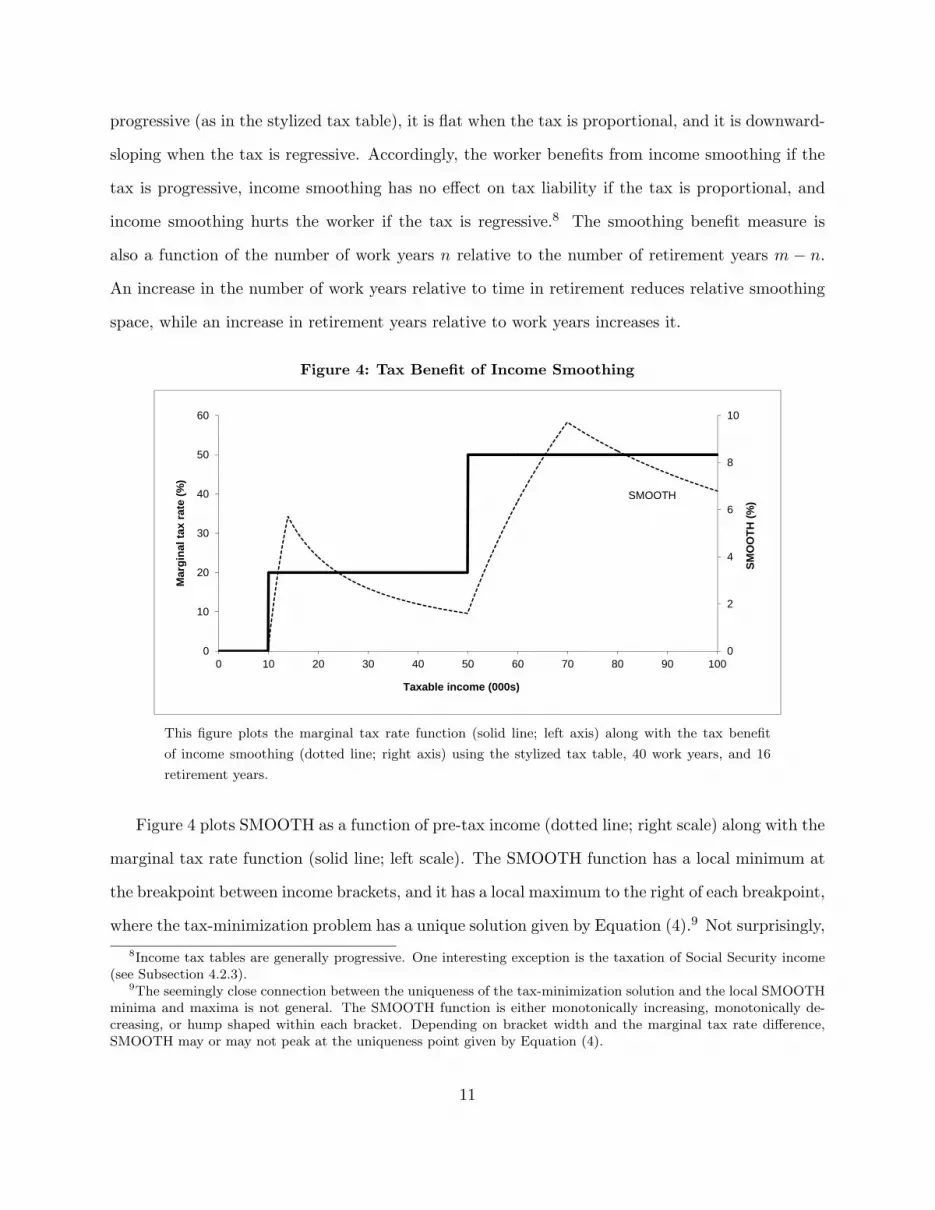
progressive (as in the stylized tax table), it is flat when the tax is proportional, and it is downward-

sloping when the tax is regressive. Accordingly, the worker benefits from income smoothing if the

tax is progressive, income smoothing has no effect on tax liability if the tax is proportional, and

income smoothing hurts the worker if the tax is regressive.8 The smoothing benefit measure is

also a function of the number of work years n relative to the number of retirement years m − n.

An increase in the number of work years relative to time in retirement reduces relative smoothing

space, while an increase in retirement years relative to work years increases it.

Figure 4: Tax Benefit of Income Smoothing

Figure 1

Page 1

0

2

4

6

8

10

0

10

20

30

40

50

60

0 10 20 30 40 50 60 70 80 90 100

SMO

OTH

(%)

Mar

gina

l tax

rate

(%)


SMOOTH

This figure plots the marginal tax rate function (solid line; left axis) along with the tax benefit

of income smoothing (dotted line; right axis) using the stylized tax table, 40 work years, and 16

retirement years.

Figure 4 plots SMOOTH as a function of pre-tax income (dotted line; right scale) along with the

marginal tax rate function (solid line; left scale). The SMOOTH function has a local minimum at

the breakpoint between income brackets, and it has a local maximum to the right of each breakpoint,

where the tax-minimization problem has a unique solution given by Equation (4).9 Not surprisingly,8Income tax tables are generally progressive. One interesting exception is the taxation of Social Security income

(see Subsection 4.2.3).9The seemingly close connection between the uniqueness of the tax-minimization solution and the local SMOOTH

minima and maxima is not general. The SMOOTH function is either monotonically increasing, monotonically de-creasing, or hump shaped within each bracket. Depending on bracket width and the marginal tax rate difference,SMOOTH may or may not peak at the uniqueness point given by Equation (4).

11

the tax benefit of income smoothing is most pronounced to the right of the breakpoints between

income brackets where the worker can shift income out of the higher bracket.10 For the same

reason, the smoothing benefit is particularly small right at each breakpoint where large amounts

of pre-tax income must be shifted into retirement to reach the lower income bracket.

3.1.3 Invariance Property

The multiplicity of solutions to the tax-minimization problem (1) means that the worker can vary

the savings rate or the point of time when he begins saving for retirement without reducing the

smoothing benefit. The invariance property is numerically illustrated in Figure 5. The upper plot

shows the effect of varying the beginning age.11 The number of work years is n, but the worker

postpones saving for retirement x years. With postponement, lifetime tax liability with and without

income smoothing are:

Non-Smooth = nT (Y ).

Smooth = xT (Y ) + (n− x)T ((1− φ)Y ) + (m− n)T(

(n−x)φYm−n

).

(8)

The smoothing benefit is maximized at the beginning age of 25 years but the two functions associ-

ated with $50,000 and $120,000 have long flat stretches where the smoothing benefit is invariant to

the beginning age. When pre-tax income is $120,000, the worker can postpone saving until age 55

without reducing the smoothing benefit and, for pre-tax income $50,000, the worker can wait until

four years before retirement. Of course, the required savings rate associated with such late starts

may be both economically painful and statutorily infeasible. The $70,000 function that occurs at a

local SMOOTH maximum is single-peaked. Every year of postponement means a loss of smoothing

benefits as perfect income smoothing is required to reach the maximum benefit of 9.7%.

The lower plot shows SMOOTH as a function of the savings rate. As in the upper plot, the two

functions associated with income levels $50,000 and $120,000 display long flat stretches where the10See Milligan (2003) for a related discussion (page 260, footnote 11).11Since we analyze a constant income stream over time, we can think of this model experiment as one with time-

varying marginal utility of consumption. When the worker is young and the marginal utility of consumption isrelatively high the worker does not save, and when he is old and marginal utility is low the worker behaves as inthe life-cycle model See discussions in Bernheim, Skinner, and Weinberg (2001) and Browning and Crossley (2001)related to empirical validation of the life-cycle model.

12

Figure 5: Invariance Property

-2

0

2

4

6

8

10

0 10 20 30 40 50

SMO

OTH

(%)

Savings rate (%)

Y=70,000

Y=120,000

Y=50,000

0

2

4

6

8

10

25 35 45 55 65

SMO

OTH

(%)

Age begin saving

Y=70,000

Y=120,000

Y=50,000

The figure plots the smoothing benefit against the beginning age and the savings rate, respectively,

for three different income levels. The calculations are based on the stylized tax table, 40 work years,

and 16 retirement years.

13

smoothing benefit does not depend on the savings rate, while the $70,000 function is single-peaked.

At $50,000, where smoothing space is small relative to smoothing demand, any savings rate from

8% to 40% yields the maximum smoothing benefit of 1.6%. The income level $120,000 represents

an intermediate case with the flat stretch shifted towards higher savings rates. A low savings rate

implies a low replacement ratio, and vice versa. The replacement ratio of retirement year income

to work year income is defined by:

ρ =n

m− n· φ

1− φ. (9)

For an annual income of $50,000, we have φmax = 40% and φmin = 8%. The replacement ratios

associated with these numbers are 167% and 22%, respectively. Hence, the replacement ratio can

vary within this range without reducing the smoothing benefit.

3.2 Interest and Income Growth

In this subsection, we investigate how real interest and income growth influence the tax benefit of

income smoothing. We analyze real as opposed to nominal interest and income growth because we

are interested in long-term retirement planning. In accordance with current practice, we assume

that tax tables are indexed to inflation.12

3.2.1 Interest

Interest generates capital income that fills up smoothing space in lower income brackets. Con-

sequently, the tax benefit of smoothing labor income decreases. In the limit, as the interest rate

approaches infinity, the smoothing benefit goes to zero.

Consider the interest rate r > 0. Each year, the worker pays tax and consumes the net proceeds

from (1 − φ)Y , and he saves the residual φY for retirement. The future value of the retirement

account after n work years equals:

FVn = FnφY, (10)12At times, nominal bracket creep can be important (Rydqvist, Spizman, and Strebulaev (2010)). Income tax tables

are nominally fixed over extended time periods between World War II and TRA 1986, but discrete adjustments takeplace, and formal cost-of-living indexation is introduced with TRA 1986.

14

where Fn = [(1 + r)n − 1] /r is the future-value annuity factor. The tax-minimization problem with

interest becomes:

minφ

T = nT ((1− φ)Y ) + (m− n)T(

FnφY

Am−n

). (11)

Interest enters inside the second term on the right hand side of the equation through the future-value

annuity factor Fn in the numerator and the present-value annuity factor Am−n in the denominator.

The income effect of earning real interest can be large. A one percent real interest rate raises the

future-value annuity factor from Fn = 40 to Fn = 48.9, which means that one percent real interest

compounded over 40 years is equivalent to being able to save for retirement over 8.9 more work

years. The effect on the denominator is also significant. The continued earning of real interest at

the one percent rate during retirement reduces the denominator by more than six years down from

m− n = 16 retirement years at zero interest to Am−n = 9.9 with one percent real interest.

A simple analytical solution obtains when income is perfectly smoothed over the life cycle. At

the time of retirement, the worker exchanges the balance from the retirement account for a life-

annuity to be paid over m− n retirement years. The procedure of saving a constant amount over

working years and exchanging the account balance for a life-annuity at retirement is analytically

equivalent to exchanging a work-year annuity for a lifetime annuity at the beginning of the working

career. Let An be the annuity factor over n work years and Am the corresponding annuity over

m life years. Perfect income smoothing over the life cycle means that the work-year annuity with

present value AnY equals the life annuity worth Am(1−φ)Y . The resulting before-tax savings rate

is, accordingly:

φ =Am −An

Am. (12)

This expressions implies that the savings rate decreases with the interest rate. Using the base-case

parameters above, a real interest rate of r = 1% reduces the savings rate from 28.6% to 23.1%,

and a real interest rate of r = 4% reduces it to 10.9%. Since the worker saves less, the smoothing

benefit decreases.

15

3.2.2 Income Growth

Income growth introduces income variability that tends to increase the smoothing benefit. Specif-

ically, income growth means that the worker is being pushed into higher income brackets towards

the end of his working career. The worker mitigates the higher effective taxation by increasing his

before-tax savings over time.

Formally, consider the constant growth rate g > 0, and define the future-value annuity factor

of income growth with zero interest as Gn = [(1 + g)n − 1] /g. To make the numbers comparable

with the no-growth case, we assume that the growth annuity is a mean-preserving spread of the

no-growth annuity by picking the starting income level Y0 at age 25 such that GnY0 = nY . This

assumption and the absence of capital market imperfections imply the smoothing benefit with

income growth as:

Non-Smooth =∑n

t=1 T (Yt).

Smooth = nT ((1− φ)Y ) + (m− n)T(

nφYm−n

).

(13)

The non-smooth term with income growth exceeds the non-smooth term without income growth in

Equation (5). This is an immediate consequence of the convexity of the tax liability function. The

smooth term with income growth is the same as the smooth term without growth in Equation (1).

One option facing the worker at age 25 is to exchange the growth annuity for a no-growth annuity

in the capital market and, then, solve the tax-minimization problem without growth. Since this is

the best the worker can do, the solutions to the growth and no-growth problems must be the same.

A numerical example with constant growth and perfect income smoothing can be seen in Fig-

ure 6. The worker borrows from age 25 to 34, he saves from age 35 to 64, and he dis-saves from age

65 to 81. In practice, the worker may not be able to borrow during early work years, and contribu-

tion limits may restrict how much he can save during late years. Borrowing and lending constraints

reduce the smoothing benefit, although the invariance property of the smoothing benefit function

suggests that borrowing and lending constraints are not binding over wide parameter ranges.

16

Figure 6: Income Growth

0

25

50

75

100

125

150

25 35 45 55 65 75

Perc

ent

Age

Save

Dis-saveBorrow

The figure shows the annual income (solid line) and annual income smoothed over adult life time

(dotted line). The growth rate is 2.5%.

3.2.3 Smoothing with Interest and Income Growth

Interest and income growth move the smoothing benefit in opposite directions. The net effect

depends on parameters and income level. In Figure 7, we plot the smoothing benefit against taxable

income assuming zero interest and no income growth (solid line), real interest rate r = 3% (dashed

line below), and real growth rate g = 3% (dashed line above). The smoothing benefit decreases

with interest, and it increases with income growth. The effect of interest is most pronounced at

each local SMOOTH maximum. The effect is also large at high income levels because high income

earners save more and interest on larger savings fill up fixed smoothing space in lower income

brackets, thus preventing the worker from smoothing labor income. The effect of income growth

is the largest at the local SMOOTH minima. Elsewhere, at very low income levels, income growth

does not push the worker into the higher bracket and, at very high income levels, taxable income

quickly fills up the fixed smoothing space anyway.

17

Figure 7: Smoothing with Interest and Income Growth

0

2

4

6

8

10

12

0 10 20 30 40 50 60 70 80 90 100

SMO

OTH

(%)


r=3%

g=3%

The figure plots the smoothing benefit as a function of taxable income assuming zero interest and

no growth (base case; solid thick line), 3% interest (dashed line below), and 3% growth (dashed

line above). The calculations are based on the stylized tax table, 40 work years, and 16 retirement

years.

3.3 Uncertainty

We conclude the analysis of the model and the stylized tax table by investigating how uncertainty

influences the tax benefit of income smoothing. A simple analytical experiment is conducted.

In the middle of his career, the worker experiences an income shock. We reach the somewhat

surprising insight that uncertainty is largely irrelevant to the smoothing benefit even for large and

unpredictable income shocks.

We analyze uncertainty by assuming that, after k work years, income jumps up or down by a

parameter λ ∈ [0, 1] with equal probability, such that:

Yu = Y (1 + λ), probability = 0.50,

Yd = Y (1− λ), probability = 0.50.(14)

The experiment is designed so that income in each state is more variable than under the base case

but the smoothing benefit may increase or decrease relative the base case depending on the income

18

level and the state of the world. The smoothing benefit is not a monotonic function of income, so

the average of the smoothing benefit evaluated at Yu and Yd, respectively, may end up larger or

smaller than the smoothing benefit evaluated at Y . To proceed, we first need to establish a full

certainty benchmark against which we can compare the effects of uncertainty.

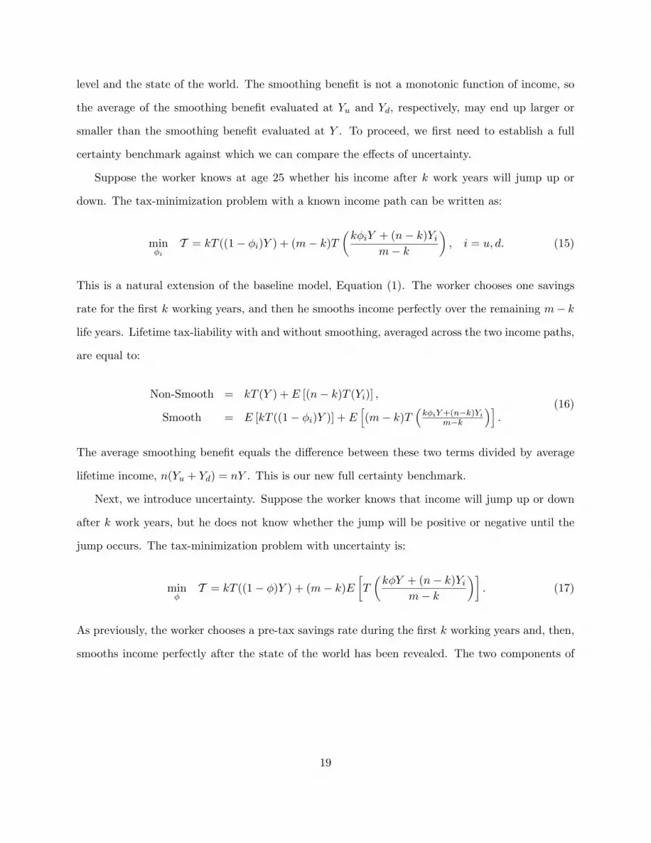
Suppose the worker knows at age 25 whether his income after k work years will jump up or

down. The tax-minimization problem with a known income path can be written as:

minφi

T = kT ((1− φi)Y ) + (m− k)T(

kφiY + (n− k)Yi

m− k

), i = u, d. (15)

This is a natural extension of the baseline model, Equation (1). The worker chooses one savings

rate for the first k working years, and then he smooths income perfectly over the remaining m− k

life years. Lifetime tax-liability with and without smoothing, averaged across the two income paths,

are equal to:

Non-Smooth = kT (Y ) + E [(n− k)T (Yi)] ,

Smooth = E [kT ((1− φi)Y )] + E[(m− k)T

(kφiY +(n−k)Yi

m−k

)].

(16)

The average smoothing benefit equals the difference between these two terms divided by average

lifetime income, n(Yu + Yd) = nY . This is our new full certainty benchmark.

Next, we introduce uncertainty. Suppose the worker knows that income will jump up or down

after k work years, but he does not know whether the jump will be positive or negative until the

jump occurs. The tax-minimization problem with uncertainty is:

minφ

T = kT ((1− φ)Y ) + (m− k)E[T

(kφY + (n− k)Yi

m− k

)]. (17)

As previously, the worker chooses a pre-tax savings rate during the first k working years and, then,

smooths income perfectly after the state of the world has been revealed. The two components of

19

the smoothing benefit measure are:

Non-Smooth = kT (Y ) + E [(n− k)T (Yi)] ,

Smooth = kT ((1− φ)Y ) + E[(m− k)T

(kφY +(n−k)Yi

m−k

)].

(18)

When we compare the average smoothing benefit with known income paths in Equation (16) to

the smoothing benefit under uncertainty in Equation (18), we see that the non-smooth terms are

equivalent, but that the smooth terms depend on the solutions φu and φd versus φ. However, the

multiplicity of solutions implies that the smooth terms may be equal. Suppose that:

φu ≤ φ ≤ φd, ∀ Y. (19)

In this case, the tax-minimizing savings rate under uncertainty is chosen where the range conditional

on being in the up-state overlaps with the range conditional on the down-state. Tax liability is

minimized in both states of the world and uncertainty is irrelevant.

In Figure 8, we plot the smoothing benefit against taxable income using our stylized tax table.

We compare the base case (5) (solid line) to known income variability (16) (dashed line) and

uncertainty (18) (same dashed line) assuming a jump parameter of λ = 0.5 after k = 20 years.

The stylized tax table and the symmetric income jump imply that the smoothing benefit with

known income variability (16) equals the smoothing benefit under uncertainty (18). Hence, the

condition (19) is satisfied and uncertainty does not reduce the smoothing benefit. We also see

that the smoothing benefit is different from the base case with a constant income stream, but the

overall impression is that the sizable jump after 20 years makes little difference. In the income

range around the local smooth minimum at Y = 50, 000, income variability raises the smoothing

benefit, and around the local smooth maxima at Y = 14, 000 and Y = 70, 000, income variability

lowers it. Over the income range displayed in Figure 8, income variability increases the average

smoothing benefit by half a percentage point.

A numerical example helps to illustrate why uncertainty does not matter. The starting income

is Y = 70, 000. After k = 20 years, income either increases to Yu = 105, 000 or decreases to

20

Figure 8: Smoothing Benefit, Income Variability, and Uncertainty

0

2

4

6

8

10

0 10 20 30 40 50 60 70 80 90 100

SMOOTH

(%)


Base case

Uncertainty & Income variability

The figure shows the smoothing benefit as a function of income using the stylized tax table under

the base case parameters, the average smoothing benefit with certain but variable income, and the

expected smoothing benefit with uncertainty. We assume 40 work years and 16 retirement years.

The jump parameter is λ = 0.5 after k = 20 years.

Yd = 35, 000. Suppose the worker knows that the down-state will occur. Anticipating the future

loss of income, the worker saves at least 20,000 per year during the first 20 years to move himself

out of the top income bracket. This saving generates a taxable income of 50,000 during the first

20 years and approximately 30,500 per year during the remaining 20 work years and 16 retirement

years. The worker can save much more, up to 55,000 per year the first 20 years, without raising

lifetime tax liability. This amount would result in an income of 15,000 during the first 20 work

years and 50,000 during the remaining 36 life years, also keeping worker out of the top income

bracket. Suppose instead that the up-state occurs. Anticipating the future salary increase, the

worker saves up to 20,000 per year resulting in taxable income of 50,000 during the first 20 years

and approximately 86,100 during the remaining 36 life years. Any higher savings amount would

waste available smoothing space the first 20 years. We see from this example that the minimum

savings amount in the down-state equals the maximum savings amount in the up-state (20,000

per year). When the worker does not know in advance which state will occur, he chooses exactly

this amount, which minimizes tax liability in the down-state and the up-state. Consequently, tax

21

liability is minimized regardless of which state occurs, and uncertainty is irrelevant.

Irrelevance is an implication of the invariance property of the smoothing benefit function (see

Subsection 3.1.3). The stylized tax table with wide income brackets allows the worker to vary the

savings rate without reducing the smoothing benefit. In experiments with asymmetric probabilities

and income jumps, we identify income regions where uncertainty makes a difference, but the effects

are small as long as we use the stylized tax table. We have also evaluated the effects of uncertainty

using a stylized tax table where the constant marginal tax rate in the middle income bracket is

replaced by a linear and continuous function. This change produces a unique solution to the tax-

minimization problem, and uncertainty matters in the middle income region. The quantitative

effects remain small, however.13

4 Income Smoothing in the United States

4.1 United States 2010

In this section, we quantify the tax benefit of income smoothing in the United States using the

2010 federal income tax table. The smoothing benefit is evaluated for a married couple filing jointly

taking the standard deduction and two exemptions. The personal exemption is higher for elderly

of age 65 and above. We make no attempt to account for the effects of progressive state and local

taxes as they vary widely across the United States.14 Many households can do better than the

standard deduction by itemizing mortgage interest, state and property taxes, etc., and they can

also claim exemptions for children. We ignore these tax deductions as they are household and time

specific, but we think including them would reduce the smoothing benefit. For example, exemptions

for children can be claimed during work years, but do not travel to retirement. Contribution limits

are not binding except in the analysis of the catch-up provision in Subsection 4.2.2.

The federal tax rate schedule up to $500,000 (left axis) along with the smoothing benefit (right

axis) can be seen in Figure 9. The smoothing benefit is about two percent at low income levels, and13A detailed description of those calculations are available from the authors upon request.14By ignoring state and local taxes, we implicitly ignore the option to move from a high-tax state during work

years to a zero-tax state in retirement.

22

Figure 9: Income Smoothing in the United States 2010

0

1

2

3

4

5

0

10

20

30

40

50

0 100 200 300 400 500

SMO

OTH

(%)

Mar

gina

l tax

rate

(%)


This figure plots the federal tax rate schedule for a married couple filing jointly taking the stan-

dard deduction and two exemptions (solid line; left axis) and the tax benefit of income smoothing

assuming 40 work years, 16 retirement years, no interest, and no income growth.

it fluctuates between three and four percent from $100,000 to $500,000. The average smoothing

benefit in this income range is 3.2%. The smoothing benefit is smaller than in the stylized tax

table in Figure 4 above, which we purposely made more progressive. The smoothing benefit is

sensitive to the income level around the breakpoint between the 15% and 25% income brackets.

Otherwise, it is approximately constant. Maximum SMOOTH occurs at annual income $125,000,

where the worker can shift all his income from the 25% bracket into the two lower brackets and the

tax-exempt smoothing space created by the standard deduction and personal exemptions.

As an example, suppose a worker has a pre-tax income of $100,000 per year. Without smoothing,

annual federal income tax liability is $12,138 during employment and $0 during retirement. With

smoothing, annual federal income tax liability is $6,742 during both employment and retirement.

The lifetime savings from income smoothing is 40 × $12, 138 − 56 × $6, 742 = $107, 960 or $2,699

per work year. These tax savings represent 2.699% of income and therefore SMOOTH=2.699%.

Hence, smoothing reduces the effective tax rate from 12.138% to 9.439%.

In Table 1, we quantify the sensitivity of the smoothing benefit to the savings rate. The

23

Table 1: Smoothing Benefit and Savings Rate

Smoothing benefit target

Perfect smoothing Max (3.2%) 3% 2% 1%

Minimum savings rate (%) 28.6 19.2 15.5 8.2 4.0

The table reports the average minimum percentage savings rate to reach a smoothing benefit target. The savingsrate and the number of years have been evaluated in increments of $1000 between $100,000 and $500,000 usingthe Federal tax table 2010 for a married couple filing jointly taking the standard deduction and two exemptions.The demographic parameters are 40 work years and 16 retirement years.

table reports the minimum savings rate that yields a targeted smoothing benefit. We evaluate the

smoothing benefit for each increment of $1000 between $100,000 and $500,000 and compute the

arithmetic average. The calculations are limited to the income range from $100,000 to $500,000

where the smoothing benefit is approximately independent of income level. The chosen range is also

where we think saving privately inside a retirement matters. Perfect income smoothing requires

that the worker saves 28.6% of his before-tax income. If this contribution rate is high, the worker

can reduce the savings rate to 19.2% without lowering the smoothing benefit. A savings rate of

19.2% may still be too high. In this case, the worker can generate smoothing benefits in the amount

of three, two, and one percent by reducing the savings rate to 15.5%, 8.2%, and 4.0%, respectively.

The two higher numbers are in line with the contribution rates of standard 401(k) contracts that,

accordingly, generate smoothing benefits of two to three percent.

4.2 Extensions

We proceed by examining the sensitivity of the smoothing benefit calculations to life expectancy

and the number of work years. In the last subsection, we introduce Social Security and examine

how retirement income from the Social Security Administration changes our calculations.

4.2.1 Life Expectancy

Smoothing space depends on life expectancy. We have chosen to work with m = 81, but the National

Center for Health Statistics provides us with numerous alternative life expectancy numbers. In

24

Table 2, we report life expectancy statistics and associated smoothing benefits conditional on

statistical method, gender, and whether the individual has reached age 25 or age 65. For a married

couple, we also report the joint and last survivor life expectancy conditional on both spouses

reaching 65 years old. The period method is based on realized life expectancy, while the cohort

method is based on life expectancy forecasts that take life expectancy growth into account. The

Table 2: Smoothing Benefit and Life Expectancy

Conditional on age 30 Conditional on age 65

Period Cohort Period Cohort Joint

A. Male

Life expectancy (years) 76.9 82.4 81.8 85.9 92.1

Smoothing benefit (%) 2.5 3.4 3.3 4.0 5.0

B. Female

Life expectancy (years) 80.9 85.9 84.2 88.4 92.1

Smoothing benefit (%) 3.2 4.0 3.7 4.4 5.0

The table shows select life expectancy statistics from the National Center for Health Statistics. The periodmethod is based on realizations, while the cohort method forecasts life expectancy growth. The smoothingbenefit has been evaluated for annual income in increments of $1000 between $100,000 and $500,000 using theFederal tax table 2010 for a married couple filing jointly taking the standard deduction and two exemptions.The table reports the arithmetic average smoothing benefit.

tabulated life expectancy statistics vary widely from 76.9 to 92.1, and the associated smoothing

benefits from 2.5% to 5.0%. Our choice of m = 81 puts us somewhere in the middle. Adding eleven

years of life expectancy raises the average smoothing benefit from 3.2% to 5.0%, and subtracting

four years reduces it to 2.5%. While longevity raises the smoothing benefit, we conclude that the

order of magnitude does not depend on which life expectancy number we pick.

4.2.2 Catch-Up Provision

Smoothing space also depends on when the worker starts saving for retirement. Starting late

unambiguously reduces the lifetime tax benefit of income smoothing (see Subsection 3.1.3 above)

but, regarding the lost years as sunk, the tax incentive to smooth income increases with age because

relative smoothing space increases. Consider a worker who did not save for retirement when young

25

and, suddenly, becomes aware of the retirement problem at age 50. The catch-up provision in the

tax code is designed for this scenario. In 2010, the 401(k) limit is $49,000 per year. This limit

applies to employer-sponsored programs.15 In addition, a worker can contribute on his own an

additional $16,500 plus the catch-up contribution amount of $5,500 from age 50. How large is the

smoothing benefit for someone who misses out the first 25 years? The fifty-year old worker has

15 remaining work years to support 16 retirement years. With no other income during retirement,

there is plenty of smoothing space relative to demand. In fact, smoothing space may be so abundant

that the worker cannot take full advantage of the smoothing benefit within statutory contribution

limits.

Table 3: Catch-Up Provision

Smoothing benefit target

Income Statutory Perfect Max 5% 4% 3% 2% 1%limit smoothing (5.5%)

$100,000 71.0 51.6 40.2 33.0 19.2 12.5 8.0 4.0

$200,000 35.5 51.6 47.4 22.5 16.0 10.7 7.1 3.5

$300,000 23.7 51.6 47.3 19.9 14.3 9.8 6.0 3.0

$400,000 17.8 51.6 42.5 21.7 16.1 10.6 6.1 2.9

$500,000 14.2 51.6 49.1 22.8 15.7 10.7 6.2 2.8

The table reports average percentage minimum savings rates at various targeted smoothing benefits for a workerwho begins saving at age 50 to support consumption during 16 retirement years. Italicized savings rates areinfeasible under statutory contribution limits. The savings rates have been evaluated using the Federal taxtable 2010 for a married couple filing jointly taking the standard deduction and two exemptions.

Smoothing benefit calculations for a fifty-year old late starter can be found in Table 3. The

percentage contribution limit and the minimum savings rate to reach a smoothing benefit target are

reported at five income levels. We obtain a percentage contribution limit by adding the 401(k) and

the elective dollar limits and dividing by annual income.16 Italicized savings rates are statutorily15There are also limitations on how much can be contributed to and paid out from a defined benefit plan, but these

limits are difficult to translate into a savings rate.16The 401(k) contribution limit is an upper boundary. Standard pension contracts specify a percentage contribution

rate that is equal to all workers with certain characteristics. A typical worker has no bargaining power over thestandard contract and must accept the contribution rate whether he reaches the $49,000 contribution limit or not.The 50-year-old worker has full discretion over the elective $22,000 amount, however.

26

infeasible. The smoothing benefit peaks between five and six percent, but such high smoothing

benefits are not statutorily feasible except at the lowest income reported in the table. A four-

percent smoothing benefit is feasible from $100,000–$400,000. For this category of late starters,

the tax incentive to smooth income is higher than for those who start at age 25. Otherwise, as the

smoothing benefit target decreases, savings rates become statutorily feasible, but the smoothing

benefit does not exceed that of early retirement savers in Figure 9.

4.2.3 Social Security

Social Security is a government-sponsored program in the United States that provides support for

individuals in times of hardship such as death of a spouse, disability, and old age (retirement). The

program is supported by a 6.2% payroll tax paid by the employee and a 6.2% payroll tax paid by

employers, both capped at wages of $106,800 in 2010. In our analysis, we ignore the contribution

component and treat the income received from the Social Security system as exogenous. To the

extent that Social Security income is taxable, it fills up smoothing space with non-labor income

thereby reducing the tax benefit of income smoothing. The effect of taxable Social Security on the

smoothing benefit is qualitatively similar to the effect of real interest (Subsection 3.2.1).

The taxation of Social Security income differs from the taxation of ordinary income. Up to

85% of Social Security income is taxable under current tax laws. The percentage depends on the

amount of other income received in retirement and Social Security income. To determine the taxed

portion of Social Security income, we first define combined income:

Y ′(φ) =nφY

m− n+ 0.5Ys, (20)

where the first term is the amount of private retirement income given by our model and the second

term is half the Social Security income. The taxed portion of Social Security income is determined

27

by the following function:

Y τs (φ) =

0, if Y ′(φ) ≤ $32, 000,

min[0.50(Y ′(φ)− $32, 000), 0.50Ys], if $32, 000 < Y ′(φ) ≤ $44, 000,

min[0.85(Y ′(φ)− $44, 000) + $6, 000, 0.85Ys], if Y ′(φ) > $44, 000.

(21)

Social Security income is tax free at low income levels (first row), and it is 85% taxable at high

income levels (third row). Between the floor and the cap, the taxed portion of Social Security

income increases linearly at the rate of 50 cents per dollar between $32,000 and $44,000, and at the

rate of 85 cents per dollar above $44,000. From these definitions, we derive the income-tax basis

with private retirement income and Social Security income:

Yr(φ) =nφY

m− n+ Y τ

s (φ) (22)

These equations show that saving privately for retirement changes the taxed portion of Social

Security income.

The worker solves the following tax-minimization problem with income from Social Security:

minφ

T = nT ((1− φ)Y ) + (m− n)T (Yr(φ)) , (23)

and he picks a tax-minimizing solution φ that determines the tax benefit of income smoothing as:17

SMOOTH =[

nT (Y )nY + (m− n)Ys

]−

[nT ((1− φ)Y ) + (m− n)T (Yr(φ))

nY + (m− n)Ys

]. (24)

For our numerical calculations, we use the benefits estimator found on the Social Security web

site. As noted by the Social Security Administration, “The benefit computation is complex and

there is no simple method or table to tell you how much you may receive”. We retrieve the benefit

amount for wages in increments of $5,000 and interpolate the values between. In order to be

conservative, we assume the married couple has a single income and credit the spouse with 50% of17Curiously, in a middle-income zone, where the worker manages his private savings such that Social Security

income is either fully or 50% exempt, the tax-minimizing solution is unique.

28

the wage earners benefits.18 In Figure 10, we report the smoothing benefit with and without Social

Figure 10: Smoothing Benefit with Social Security

0

1

2

3

4

5

0 100 200 300 400 500

SMO

OTH

(%)


Social Security

Base case

The figure compares the tax benefit of income smoothing without Social Security (base case; solid

line) and with Social Security (dashed line) using the 2010 federal tax rate schedule for a married

couple filing jointly taking the standard deduction and two exemptions. The married couple has

one income, and the non-working spouse receives 50% of the wage earner’s Social Security benefit.

We assume 40 work years, 16 retirement years, no interest, and no income growth.

Security using the 2010 tax rate schedule. We see that Social Security reduces the tax benefit of

income smoothing relative to the base case by approximately one to two percentage points. The

main reason is smoothing space reduction. Taxable Social Security income fills up the lower infra-

marginal brackets that otherwise would have been available for private retirement income. At lower

income levels, a large portion of Social Security income is tax exempt and, therefore, does not fill

up smoothing space.

4.3 United States 1950–2010

We end our examination by reporting smoothing benefit numbers from the United States history

after 1950. The historical time-series allow us to compare our estimates with those of Ippolito18For married couples, the spouse with the lower earned benefits receives the greater of actual earned benefits or

50% of the spouse’s earned benefits. With two equal incomes the household receives 200% of the Social Securitybenefit of the highest income earner. Due to the progressivity of Social Security benefits, married couples may receivemore than twice the benefits of a single individual with the same income.

29

(1986). The historical numbers can also shed light on the argument that the smoothing benefit

is one of the driving forces behind the growth of the private pension system in the United States

(Ippolito (1986)).

Figure 11: Income Smoothing in the United States 1979

0

1

2

3

4

5

6

7

0

25

50

75

100

0 20 60 80 100

SMO

OTH

(%)

Mar

gina

l tax

rate

(%)


Ippolito (1986)

This figure plots the federal tax rate schedule for a married couple filing jointly taking the stan-

dard deduction and two exemptions (solid line; left axis) and the tax benefit of income smoothing

assuming 40 work years, 13 retirement years, no interest, and no income growth (dashed line; right

axis). Ippolito (1986) bases his calculations on the Statistics of Income (filled diamonds).

Ippolito (1986) bases his calculations on actual taxes paid according to Statistics of Income

rather than the Federal tax rate schedule. He assumes that work begins at age 25 and that the

worker retires at age 65 but, since life expectancy is shorter in 1979, the worker dies at age 78.

His smoothing benefit calculations are marked as diamonds in Figure 11, where we also plot the

Federal marginal tax rate schedule up to $120,000 and our smoothing benefit function using his

demographic parameters. The chosen income range corresponds in real terms to the income used

in Figure 9 for 2010 data. Our smoothing benefit numbers are a little higher than those of Ippolito

(1986), but the increasing pattern is similar.19 The smoothing benefit is generally higher in 1979

than in 2010 because the 1979 tax table is more progressive. The smoothing benefit averaged over

the income range $20,000 to $120,000 is 5.2%.19We infer these estimates from the information provided by Ippolito (1986) in Table 2-1.

30

Our historical smoothing benefit calculations are based on life expectancy statistics from the

Human Mortality Database, the average of male and female conditional on age 25.20 Tax liability is

evaluated assuming an annual income of five times GDP per capita, which is approximately $60,000

in 1979 and $230,000 in 2008 (the most recently available). This income level is relatively high

so that saving privately for retirement matters, but it is not so high that standard pension plans

become marginal. It is at the margin of the 401(k) contribution limit and statutorily feasible.21

GDP-per-capita time-series are taken from the International Financial Statistics Browser provided

by the International Monetary Fund. We compute the smoothing benefit with and without Social

Security. A worker with income equal to five times GDP per capita receives the maximum Social

Security benefit.

Figure 12: Smoothing Benefit History

0

1

2

3

4

5

6

1950 1960 1970 1980 1990 2000

SMO

OTH

(%)

Base case

Social Security

ERTA 1981

TRA 1986

The solid line above is the base case smoothing benefit assuming 40 work years and time in retire-

ment equal to life expectancy minus 65. Tax liability is evaluated at an income of five times GDP

per capita for a married couple filing jointly taking the standard deduction and two exemptions.

The dashed line below adjust for Social Security income assuming that the married couple receives

150% of the wage earner’s Social Security benefit. We have marked the Economic Recovery Tax

Act of 1981 (ERTA 1981) and the Tax Reform Act of 1986 (TRA 1986).

The post-war time-series of smoothing benefits is displayed in Figure 12. The solid line above20University of California, Berkeley (USA) available at www.mortality.org.21Contribution limits are introduced with the 401(k) plan. Previously, employers may offer any pension to their

employees (Gokhale, Kotlikoff, and Warshawsky (2004)).

31

represents our base case, and the dashed line below the smoothing benefit with Social Security.

The time-series path is hump shaped with a positive time trend. Increasing life expectancy drives

the time trend. The peak occurs shortly before the tax reform when Ippolito (1986) analyzes the

tax benefit of income smoothing. The hump is the result of bracket creep and the regulatory

response to combat it. Income tax tables are essentially unchanged from 1950 to 1980. While

personal income taxes are nominally fixed during this long thirty-year period, nominal income per

capita increases approximately six times. As a result of income growth, five times GDP per capita

grows from $10,000 in 1950 to $60,000 in 1980. The effect on the smoothing benefit can be seen in

Figure 11 above. The smoothing benefit associated with $10,000 income is about 3% (1950), while

the smoothing benefit of $60,000 is close to 6% (1980). Together with increased life expectancy,

bracket creep raises the smoothing benefit from 1% in 1950 to above 5% in 1980 as seen in Figure 12.

The tax reform (TRA 1986) reduces progressivity, and inflation indexing prevents further bracket

creep.

Social Security reduces the smoothing benefit, but the effect of Social Security changes over

time. Social Security income reduces the smoothing benefit from 1984 when it becomes partly

taxed. The gap between the cases with and without Social Security widens in 1994 when the taxed

portion increases and fills up more smoothing space.

5 Conclusion

Households can defer income taxes until withdrawal by saving before tax inside a traditional re-

tirement account. Under a progressive tax system, deferral of income tax to retirement provides

a smoothing benefit. The tax benefit of income smoothing is perceived as large. However, our

estimates for the United States in 2010 in the amount of 3.2% without Social Security and 1.7%

adjusted for Social Security are surprisingly small relative to the perceived benefit. Our calculations

are derived from solving a tax minimization problem. We have not studied what economic agents

actually do. Especially, we have not discussed the effects of smoothing on individuals’ savings

behavior or the rationale for tax policies related to pension and retirement savings. However, our

calculations suggest that the tax benefit of income smoothing is too small to explain the growth

32

of the US private pension system, as claimed by Ippolito (1986). At best, the smoothing benefit

can have inspired retirement planners and labor unions bargaining for pensions over wages during

a short time period in the 1970s, when the smoothing benefit was substantially larger than today.

33

References

Bernheim, B. Douglas, Jonathan Skinner, and Steven Weinberg, 2001, What Accounts for theVariation in Retirement Wealth among U.S. Households?, American Economic Review 91, 832–857.

Browning, Martin, and Thomas F. Crossley, 2001, What Accounts for the Variation in RetirementWealth among U.S. Households?, Journal of Economic Perspective 15, 3–22.

Burmann, Leonard E., William G. Gale, and David Weiner, 2001, The Taxation of RetirementSaving: Choosing between Front-Loaded and Back-Loaded Options, National Tax Journal 54,689–702.

Constantinides, George M., 1983, Capital Market Equilibrium with Personal Tax, Econometrica51, 611–636.

Eissa, and Hoynes, 2000, Tax and Transfer Policy, and Family Formation: Marriage and Cohabi-tation, working paper, UC Berkeley.

Feenberg, Daniel, and Jonathan Skinner, 1989, Sources of IRA Saving, Tax Policy and the Economy3, 25–46.

Gokhale, Jagadeesh, Laurence J. Kotlikoff, and Todd Neumann, 2008, Does Participation in 401(k)Raise Lifetime Taxes?, working paper, Federal Reserve Bank of Cleveland.

Gokhale, Jagadeesh, Laurence J. Kotlikoff, and Mark J. Warshawsky, 2004, Life-Cycle Saving,Limits on Contributions to DC Pension Plans, and Lifetime Tax Benefits, in William G. Gale,John. B. Shoven, and Mark J. Warshawsky, Private Pensions and Public Policies (BrookingsInstitutions Press, Washington D.C.).

Green, Richard C., and Kristian Rydqvist, 1999, Ex-Day Behavior with Dividend Preference andLimitations to Short-Term Arbitrage: The Case of Swedish Lottery Bonds, Journal of FinancialEconomics 53, 145–187.

Horan, Stephen M., 2005, Tax-Advantaged Savings Accounts and Tax-Efficient Wealth Accumula-tion. (Research Foundation of the CFA Institute).

Horan, Stephen M., 2009, Private Wealth: Wealth Management in Practice. (John Wiley & Sons,Hoboken, New Jersey).

Huang, Jennifer, 2008, Taxable and Tax-Deferred Investing: A Tax-Arbitrage Approach, Review ofFinancial Studies 21, 2173–2207.

Ippolito, Richard A., 1986, Pensions, Economics, and Public Policy. (Dow Jones-Irwin HomewoodIllinois).

Lankford, Kimberly, 2008, Taxes on 401(k) and IRA Withdrawals, available athttp://www.kiplinger.com/columns/ask/archive/2008/q0508.htm.

Lowenstein, Roger, 2008, While America Aged: How Pension Debts Ruined General Motors,Stopped the NYC Subways, Bankrupted San Diego, and Loom as the Next Financial Crisis.(Penguin Press, New York).

34

Milligan, Kevin, 2003, How Do Contribution Limits Affect Contributions to Tax-Preferred SavingsAccounts?, Journal of Public Economics 87, 253–281.

Nishiyama, Shinichi, 2010, The Budgetary and Welfare Effects of Tax-Deferred Retirement SavingsAccounts, working paper, Georgia State University.

Ozanne, Larry, and David Lindeman, 1987, Tax Policy for Pensions and other Retirement Savings,Congressional Budget Office Study, Congress of the United States.

Ragan, Christopher, 1994, Progressive Income Taxes ad the Substitution Effect of RRSPs, CanadianJournal of Economics 27, 43–57.

Reno, Virginia P., and Joni Lavery, 2007, Social Security and Retirement Income Adequacy, SocialSecurity Brief 25, pp. 1-12, National Academy of Social Insurance.

Røed, Knut, and Steinar Strøm, 2002, Progressive Taxes and the Labour Market: Is the Trade-Offbetween Equality and Efficiency Inevitable?, Journal of Economic Surveys 16, 77–110.

Rydqvist, Kristian, 2011, Tax Arbitrage with Risk and Effort Aversion: Swedish Lottery Bonds1970–1990, working paper, SSRN.

Rydqvist, Kristian, Joshua D. Spizman, and Ilya Strebulaev, 2010, The Evolution of AggregateStock Ownership, working paper, SSRN.

Slitor, Richard E., 1948, The Measurement of Progressivity and Built-In Flexibility, QuarterlyJournal of Economics 62, 309–313.

Stephens, Melvin, and Jennifer Ward-Batts, 2004, The Impact of Separate Taxation on the Intra-Household Allocation of Assets: Evidence from the UK, Journal of Public Economics 88, 1989–2007.

Stiglitz, Joseph E., 1988a, Economics of the Public Sector. (W.W. Norton & Company).

Stiglitz, Joseph E., 1988b, The general theory of tax avoidance, NBER working paper.

Turner, John A., 2005, Pensions, tax treatment of, in J. Cordes, R. Ebel, and J. Gravelle, eds.:NTA Encyclopedia of Taxation and Tax Policy (Urban Institute Press, Washington D.C.).

Vroman, Wayne, 1974, Employer Payroll Taxes and Money Wage Behavior, Applied Economics 6,189–204.

35

The tax benefit of income smoothing

Documents

Transcript of The tax benefit of income smoothing