Tilburg University

Fast Filtering and Smoothing for Multivariate State Space Models

Koopman, S.J.M.; Durbin, J.

Publication date:1998

Link to publication in Tilburg University Research Portal

Citation for published version (APA):Koopman, S. J. M., & Durbin, J. (1998). Fast Filtering and Smoothing for Multivariate State Space Models.(CentER Discussion Paper; Vol. 1998-18). Econometrics.

General rightsCopyright and moral rights for the publications made accessible in the public portal are retained by the authors and/or other copyright ownersand it is a condition of accessing publications that users recognise and abide by the legal requirements associated with these rights.

• Users may download and print one copy of any publication from the public portal for the purpose of private study or research. • You may not further distribute the material or use it for any profit-making activity or commercial gain • You may freely distribute the URL identifying the publication in the public portal

Take down policyIf you believe that this document breaches copyright please contact us providing details, and we will remove access to the work immediatelyand investigate your claim.

Download date: 12. Mar. 2022

Fast filtering and smoothing for multivariate state space modelsS.J. Koopman †Tilburg University, The Netherlands.J. DurbinLondon School of Economics and Political Science, UK.

Abstract

This paper gives a new approach to diffuse filtering and smoothingfor multivariate state space models. The standard approach treats theobservations as vectors while our approach treats each element of theobservational vector individually. This strategy leads to computation-ally efficient methods for multivariate filtering and smoothing. Also,the treatment of the diffuse initial state vector in multivariate modelsis much simpler than existing methods. The paper presents detailsof relevant algorithms for filtering, prediction and smoothing. Proofsare provided. Three examples of multivariate models in statistics andeconomics are presented for which the new approach is particularlyrelevant.

Keywords: Diffuse initialisation; Kalman filter; Multivariate model-s; Smoothing; State space; Time series.

† Address for correspondence: CentER for Economic Research, POBox 90153, 5000 LE Tilburg, The Netherlands.E-mail: s.j.koopman@kub.nl

February 1998

1

1 Introduction

In the standard multivariate linear state space model, the observation vectoryt depends linearly on an unobserved state vector αt which develops overtime as a first order vector autoregression for t = 1, . . . , n. In this paperwe consider filtering and smoothing for this model. The object of filtering isto calculate the mean and error variance matrix of αt given y1, . . . , yt−1 andthe object of smoothing is to calculate the mean and error variance matrixof αt given y1, . . . , yn. Analysis based on these models is important in manyareas and particularly in applied time series analysis. For a general treatmentof state space models for time series analysis see Harvey (1989) and for anapplication to a particular problem of public importance together with apublished discussion of the merits of these models see Harvey and Durbin(1986).

The conventional approach to filtering and smoothing for these modelsis based on considering the contribution of the entire observational vectorat each successive time point. The basic idea of this paper is to introducethe elements of the observational vectors one at a time into the filtering andsmoothing processes. In effect, we convert the original multivariate seriesinto a univariate series and analyse the data in univariate form. Although theconcept is simple, the improvement in computational efficiency is dramaticfor models of more than a modest degree of complexity. The advantage isparticularly strong for the treatment of initialisation by diffuse priors.

The idea of decomposing the observational vectors into sub-vectors for theimprovement of computational efficiency in Kalman filtering was suggestedby Anderson and Moore (1979, section 6.4) under the name sequential pro-cessing. Fahrmeir and Tutz (1994, section 8.4) discuss a similar strategy forlongitudinal models. However, both contributions assume that the initialconditions are known and they do not deal with diffuse initialisation andparameter estimation which are major concerns in this paper.

Section 2 presents the multivariate linear Gaussian state space modeland sets out the standard Kalman filter recursions in a form that is suitablefor later work in the paper. A general form of the partially diffuse initialstate vector is considered in which some elements of the state vector at theinitial time point have finite variances while others have infinite variances.In section 3 the model is written in univariate form, first for the case wherethe observation error matrix is diagonal and secondly for the case where the

2

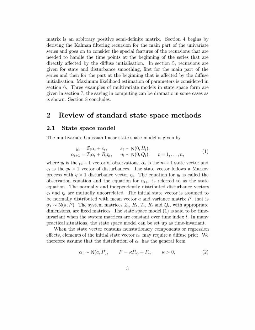
matrix is an arbitrary positive semi-definite matrix. Section 4 begins byderiving the Kalman filtering recursion for the main part of the univariateseries and goes on to consider the special features of the recursions that areneeded to handle the time points at the beginning of the series that aredirectly affected by the diffuse initialisation. In section 5, recursions aregiven for state and disturbance smoothing, first for the main part of theseries and then for the part at the beginning that is affected by the diffuseinitialisation. Maximum likelihood estimation of parameters is considered insection 6. Three examples of multivariate models in state space form aregiven in section 7; the saving in computing can be dramatic in some cases asis shown. Section 8 concludes.

2 Review of standard state space methods

2.1 State space model

The multivariate Gaussian linear state space model is given by

yt = Ztαt + εt, εt ∼ N(0, Ht),αt+1 = Ttαt +Rtηt, ηt ∼ N(0, Qt), t = 1, . . . , n,

(1)

where yt is the pt× 1 vector of observations, αt is the m× 1 state vector andεt is the pt × 1 vector of disturbances. The state vector follows a Markovprocess with q × 1 disturbance vector ηt. The equation for yt is called theobservation equation and the equation for αt+1 is referred to as the stateequation. The normally and independently distributed disturbance vectorsεt and ηt are mutually uncorrelated. The initial state vector is assumed tobe normally distributed with mean vector a and variance matrix P , that isα1 ∼ N(a, P ). The system matrices Zt, Ht, Tt, Rt and Qt, with appropriatedimensions, are fixed matrices. The state space model (1) is said to be time-invariant when the system matrices are constant over time index t. In manypractical situations, the state space model can be set up as time-invariant.

When the state vector contains nonstationary components or regressioneffects, elements of the initial state vector α1 may require a diffuse prior. Wetherefore assume that the distribution of α1 has the general form

α1 ∼ N(a, P ), P = κP∞ + P∗, κ > 0, (2)

3

where vector a and matrices P∞ and P∗ are fixed and known and where weshall in due course let κ→∞. The matrix P∞ is typically diagonal and whena diagonal element of P∞ is nonzero the corresponding row and column ofP∗ are not relevant.

2.2 Kalman filter

The Kalman filter recursions evaluate the mean of the state vector αt+1 con-ditional on the observations Yt = {y1, . . . , yt} and its error variance matrix,that is at+1 = E(αt+1|Yt) and Pt+1 = var(αt+1 − at+1|Yt), for t = 1, . . . , n.The Kalman filter for the state space model (1) and (2) with κ given can bewritten in the form

vt = yt − Ztat,

at+1 = Tt(at +KtF

−1t vt

),

Ft = ZtPtZ′t +Ht,

Kt = PtZ′t,

Pt+1 = Tt(Pt −KtF

−1t K ′t

)T ′t +RtQtR

′t,

(3)for t = 1, . . . , n. The one-step ahead prediction error is vt = yt − E(yt|Yt−1)with variance matrix Ft = var(yt|Yt−1) = var (vt). The matrix Kt is thecovariance matrix cov (αt, yt|Yt−1). The proof of the Kalman filter can beobtained by applying some basic results on the multivariate normal distribu-tion or by applying linear prediction results; see, for example, Duncan andHorn (1972), Anderson and Moore (1979) and Harvey (1989).

The Kalman filter recursions for given κ are initialised by

a1 = E (α1|Y0) = E (α1) = a, P1 = var (α1|Y0) = var (α1) = P, (4)

where a and P are the unconditional mean and variance matrix of the initialstate vector, respectively. The diffuse case of κ → ∞ is discussed when weconsider the univariate form of the filter in section 4.2.

2.3 Smoothing

Estimators of the state and disturbance vectors, conditional on the full set ofobservations Yn = {y1, . . . , yn}, are referred to as smoothed estimators andthey are evaluated by backwards smoothing algorithms. The work of de Jong(1988), Kohn and Ansley (1989) and Koopman (1993) leads to the following

4

basic smoothing recursions for model (1),

rt−1 = Z ′tF−1t vt + L′tT

′trt, Nt−1 = Z ′tF

−1t Zt + L′tT

′tNtTtLt, (5)

for t = n, . . . , 1 with Lt = I −KtF−1t Zt. The backwards recursions (5) are

initialized by rn = 0 and Nn = 0. Storage of the Kalman filter output vt,F−1t and Kt is required for t = 1, . . . , n.

The output of recursions (5) can be used to construct the smoothed es-timators of the disturbance vectors εt and ηt conditional on the full data-setYn, that is εt = E (εt|Yn) and ηt = E (ηt|Yn), together with their variancematrices. These smoothed estimators are computed by

εt = HtF−1t (vt −K ′trt) , var (εt) = HtF

−1t (Ft +K ′tNtKt)F

−1t Ht,

ηt = QtR′trt, var (ηt) = QtR

′tNtRtQt,

(6)for t = n, . . . , 1. The proofs and more general results for smoothed distur-bances are given by Koopman (1993).

The smoothed state vector αt = E (αt|Yn) and variance matrix Vt =var (αt|Yn) also use (5) and can be evaluated by

αt = at + Ptrt−1, Vt = Pt − PtNt−1Pt, (7)

for t = n, . . . , 1. A substantial amount of additional memory space is requiredfor the storage of at and Pt. Proofs of (5) and (7) are given by de Jong (1988)and Kohn and Ansley (1989). The state smoother (5) and (7) can also beobtained by re-formulating the classical Anderson and Moore (1979) fixedinterval smoothing algorithm; see Koopman (1997b).

A more efficient algorithm for calculating the smoothed estimator of thestate vector only is given by

αt+1 = Ttαt +Rtηt, t = 1, . . . , n, (8)

with α1 = a + Pr0 and ηt is given by (6). The forwards recursion (8) canbe applied after the smoothing algorithm (5) has stored the vector rt usingthe storage space of the Kalman filter, for t = 1, . . . , n. The substantialstorage space for the state smoother (7) is not required. Also, the recursion(8) is computationally more efficient than the first equation of (7) becausethe matrices Tt and Rt in (8) are usually sparse; see Koopman (1993) for adiscussion.

5

3 Univariate approach to multivariate case

Assuming first that variance matrix Ht is diagonal, write the observation andobservation disturbance vectors as

yt =

yt,1...

yt,pt

, εt =

εt,1...

εt,pt

,with the observation system matrices

Zt =

Zt,1

...Zt,pt

, Ht =

σ2t,1 0 0

0. . . 0

0 0 σ2t,pt

,where yt,i, εt,i and σ2

t,i are scalars and Zt,i is a (1 ×m) row vector, for i =1, . . . , pt. The observation equation for the univariate representation of themodel is

yt,i = Zt,iαt,i + εt,i, t = 1, . . . , n, i = 1, . . . , pt, (9)

where αt,i = αt. The state equation corresponding to (9) is

αt,i+1 = αt,i, i = 1, . . . , pt − 1,αt+1,1 = Ttαt,pt +Rtηt, t = 1, . . . , n,

(10)

with initial state vector α1,1 = α1 given by (2).When Ht is not diagonal, we put the disturbance vector εt into the state

vector. For the observation equation of (1) define

αt =

(αtεt

), Zt =

(Zt Imt

),

and for the state equation define

ηt =

(ηtεt

), Tt =

(Tt 00 0

), Rt =

(Rt 00 Imt

), Qt =

(Qt 00 Ht

),

leading to

yt = Ztαt, αt+1 = Ttαt + Rtηt, ηt ∼ N(0, Qt),

for t = 1, . . . , n. We then proceed with the same strategy as for the case whereHt is diagonal by treating each element of the observation vector individually.

6

4 Univariate filtering

4.1 The basic algorithm

Define at,1 = E (αt,1|Yt−1) and at,i = E (αt,i|Yt−1, yt,1, . . . , yt,i−1) with Pt,1 =var (αt,1|Yt−1) and Pt,i = var (αt,i|Yt−1, yt,1, . . . , yt,i−1), for i = 2, . . . , pt. Bytreating the vector series y1, . . . , yn as the scalar series

y1,1, . . . , y1,pt, y2,1, . . . , yn,pn,

the filtering equations where Ht is diagonal can be written as

at,i+1 = at,i +Kt,iF−1t,i vt,i, Pt,i+1 = Pt,i −Kt,iF

−1t,i K

′t,i, (11)

where

vt,i = yt,i − Zt,iat,i, Ft,i = Zt,iPt,iZ′t,i + σ2

t,i, Kt,i = Pt,iZ′t,i, (12)

for i = 1, . . . , pt and t = 1, . . . , n. This formulation has vt,i and Ft,i as scalarsand Kt,i as a column vector. The transition from time t to time t + 1 isachieved by the relations

at+1,1 = Ttat,pt+1, Pt+1,1 = TtPt,pt+1T′t +RtQtR

′t. (13)

These values at+1,1 and Pt+1,1 are the same as the values at+1 and Pt+1 givenby the standard Kalman filter (3).

It is important to note that the elements of the innovation vector vt of (3)are not the same as vt,i, for i = 1, . . . , pt; only the first element of vt is equalto vt,1. The same applies to the diagonal elements of the variance matrix Ftand the variances Ft,i, for i = 1, . . . , pt; only the first diagonal element of Ftis equal to Ft,1. It is reasonable to assume that the full matrix Ft is not zerosince this would indicate a model that had not been properly formulated.However, there are models for which Ft,i can be zero, for example the casewhere yt is a multinomial observation. This indicates that yt,i is linearlydependent on previous observations. Thus

at,i+1 = E (αt,i+1|Yt−1, yt,1, . . . , yt,i) = E (αt,i+1|Yt−1, yt,1, . . . , yt,i−1) = at,i,

and similarly Pt,i+1 = Pt,i. The contingency is therefore easily dealt with.

7

The main motivation of this ‘univariate’ approach to filtering for multi-variate state space models is computational efficiency. This approach avoidsthe inversion of matrix Ft and two matrix multiplications. Also, the actu-al implementation of the recursions is more straightforward. Table 1 showsthat the percentage savings in the number multiplications for the univariateapproach compared to the standard approach are considerable. The calcula-tions concerning the transition (13) are not considered because matrix Tt isusually sparse with most elements equal to zero and unity.

4.2 Diffuse filtering

The filtering recursions (11) to (13) are valid for initial condition (2) withany fixed κ > 0. The diffuse case of κ → ∞ requires some adjustmentsfor a limited number of filtering steps until the dependence of Pt,i on κ hasvanished. The method of diffuse initialisation is based on the treatment ofKoopman (1997a).

The definition P = P∗ + κP∞ in (2) implies that the matrix Pt,i, thevector Kt,i and the scalar Ft,i, can be decomposed as

Pt,i = P∗,t,i + κP∞,t,i,

Kt,i = K∗,t,i + κK∞,t,i, (14)

Ft,i = F∗,t,i + κF∞,t,i,

where

F∗,t,i = Zt,iP∗,t,iZ′t,i + σ2

t,i, F∞,t,i = Zt,iP∞,t,iZ′t,i,

K∗,t,i = P∗,t,iZ′t,i, K∞,t,i = P∞,t,iZ

′t,i.

(15)

To obtain the diffuse filtering recursions, we expand F−1t,i as a power series in

κ−1 giving

F−1t,i = κ−1F−1

∞,t,i − κ−2F∗,t,iF

−2∞,t,i +O

(κ−3

), for F∞,t,i > 0.

This is easily obtained from the identity F−1t,i (F∗,t,i + κF∞,t,i) = 1; see Koop-

man (1997a). From (11) the diffuse filtering recursions are therefore givenby

at,i+1 = at,i +K∞,t,iF−1∞,t,ivt,i,

8

P∗,t,i+1 = P∗,t,i +K∞,t,iK′∞,t,iF∗,t,iF

−2∞,t,i − (16)(

K∗,t,iK′∞,t,i +K∞,t,iK

′∗,t,i

)F−1∞,t,i,

P∞,t,i+1 = P∞,t,i −K∞,t,iK′∞,t,iF

−1∞,t,i,

for i = 1, . . . , pt. In the case where F∞,t,i = 0, the usual filtering equationsapply, that is

at,i+1 = at,i +K∗,t,iF−1∗,t,ivt,i,

P∗,t,i+1 = P∗,t,i −K∗,t,iK′∗,t,iF

−1∗,t,i, (17)

P∞,t,i+1 = P∞,t,i,

for i = 1, . . . , pt. For the transition from time t to time t+ 1 we have

at+1,1 = Ttat,pt+1,

P∗,t+1,1 = TtP∗,t,pt+1T′t +RtQtR

′t, (18)

P∞,t+1,1 = TtP∞,t,pt+1T′t ,

for t = 1, . . . , n.Although it is not a restriction for a properly defined model, we require

thatr (P∞,t+1,1) = r (P∞,t,pt+1) , (19)

which implies that matrix Tt does not influence the rank of P∞,t,i. It can beshown that, when F∞,t,i > 0,

r (P∞,t,i+1) = r (P∞,t,i)− 1; (20)

see Koopman (1997a). The diffuse recursions (16) to (18) are continued untilmatrix P∞,t,i+1 becomes zero at t, i = t∗, i∗. From then on the usual Kalmanfilter is used with Pt,i+1 = P∗,t,i+1. The univariate series

y1,1, . . . , y1,pt, y2,1, . . . , yt∗,i∗

will be referred to as the initial series.It can be shown that, when F∞,t,i > 0, the filtering recursion (16) for

P †t,i = (P∗,t,i, P∞,t,i) can be written compactly as

P †t,i+1 = L†tP†t,i, with L†t =

(L∞,t,i Lo,t,i0 L∞,t,i

), i = 1, . . . , pt, (21)

9

where

L∞,t,i = I −K∞,t,iZt,iF−1∞,t,i,

Lo,t,i =(K∞,t,iF∗,t,iF

−1∞,t,i −K∗,t,i

)Zt,iF

−1∞,t,i; (22)

see Koopman and Durbin (1998, section 4).The diffuse filtering equations imply a limited number of additional multi-

plications compared to the usual Kalman filter. The computational implica-tions are discussed in Koopman (1997a) where it is argued that this methodoutperforms existing methods for univariate cases. It should be stressed thatour approach of diffuse multivariate filtering is simpler and computationallymore efficient than the methods proposed by Ansley and Kohn (1985) andKoopman (1997a) which require intricate Cholesky transformations on vari-ance matrices such as Pt and Ft. Our approach also outperforms the diffuseinitialisation methods of de Jong (1991) and Snyder and Saligari (1996) forunivariate and multivariate cases.

5 Univariate smoothing

5.1 The basic algorithm

The basic smoothing recursions (5) for the model (1) can be reformulated forthe univariate series

y1,1, . . . , y1,pt, y2,1, . . . , yn,pn,

as

rt,i−1 = Z ′t,iF−1t,i vt,i + L′t,irt,i, Nt,i−1 = Z ′t,iF

−1t,i Zt,i + L′t,iNt,iLt,i,

rt−1,pt = T ′t−1rt,0, Nt−1,pt = T ′t−1Nt,0Tt−1,(23)

where Lt,i = I −Kt,iZt,iF−1t,i , for i = pt, . . . , 1 and t = n, . . . , 1. The initiali-

sations are rn,pn = 0 and Nn,pn = 0. The equations for rt−1,pt and Nt−1,pt donot apply for t = 1. The values for rt,0 and Nt,0 are the same as the valuesfor the smoothing quantities rt−1 and Nt−1 of (5), respectively.

The univariate smoothing approach avoids two matrix multiplications andthe implementation is more straightforward. Table 2 presents the consider-able percentage savings in the number of multiplications for the univariate

10

approach compared to the standard multivariate approach. The computa-tions involving the usually sparse transition matrix Tt are not considered.

5.2 State and disturbance smoothing

The state smoothing equations for our ‘univariate’ approach provide the sameresults as equations (7) since at = at,1, Pt = Pt,1, rt−1 = rt,0 and Nt−1 = Nt,0.Similar considerations apply for the smoothed disturbances ηt and var (ηt) in(6) and the state smoother (8). The smoothed estimators for the observationdisturbances εt,i of (9) follow directly from our approach and are given by

εt,i = σ2t,iF

−1t,i

(vt,i −K ′t,irt,i

), var (εt,i) = σ4

t,iF−2t,i

(Ft,i +K ′t,iNt,iKt,i

).

5.3 Diffuse smoothing

In this section we present the diffuse smoothing recursions for the initialseries with indices

(t, i) = (t∗, i∗) , (t∗, i∗ − 1) , . . . , (t∗, 1) , (t∗ − 1, pt∗−1) , . . . , (1, 1) .

The treatment is based on Koopman and Durbin’s (1998) results for thevector observation case.

To obtain smoothed estimators as κ→∞, we expand rt,i and Nt,i of (23)in terms of reciprocals of κ in the same way as for F−1

t,i , that is

rt,i = r(0)t,i + κ−1r

(1)t,i +O

(κ−2

),

Nt,i = N(0)t,i + κ−1N

(1)t,i + κ−2N

(2)t,i +O

(κ−3

), (24)

with r(0)t∗,i∗ = rt∗,i∗, r

(1)t∗,i∗ = 0, N

(0)t∗,i∗ = Nt∗,i∗ and N

(1)t∗,i∗ = N

(2)t∗,i∗ = 0. We need

three terms in the series for Nt,i compared with two in the series for rt,i toallow for the contribution of terms in κ and κ2 from the multiplications ofPt = P∗,t + κP∞,t required for state smoothing as given by (7). Note thatrt∗,i∗ and Nt∗,i∗ are obtained from (23) at t, i = t∗, i∗. By defining

r†t,i =

(r

(0)t,i

r(1)t,i

), N †t,i =

(N

(0)t,i N

(1)t,i

N(1)t,i N

(2)t,i

),

11

it can be shown using (23) that the diffuse basic smoothing equations, whenF∞,t,i > 0, are given by

r†t,i−1 =

(0

Z ′t,iF−1∞,t,ivt,i

)+ L†′t,ir

†t,i,

N †t,i−1 =

(0 Z ′t,iF

−1∞,t,iZt,i

Z ′t,iF−1∞,t,iZt,i Z ′t,iF

−2∞,t,iZt,iF∗,t,i

)+ L†′t,iN

†t,iL†t,i, (25)

where L†t,i is defined as in (21) for the initial series and with

r†t−1,pt =

(Tt−1 00 Tt−1

)′r†t,0,

N †t−1,pt =

(Tt−1 00 Tt−1

)′N †t,0

(Tt−1 00 Tt−1

),

for t = t∗, . . . , 1; see section 4 of Koopman and Durbin (1998) for details.The diffuse state smoothing equations are given by

αt = at,1 + P †t,1r†t,0, Vt = P∗,t,1 − P

†t,1N

†t,0P

†′t,1, (26)

for t = t∗, . . . , 1. The diffuse smoothed disturbances for the initial series aregiven by

εt,i = −σ2t,iF

−1∞,tK

′∞,tr

(0)t,i , var (εt,i) = σ4

t,iF−2∞,tK

′∞,tN

(0)t,i K∞,t,

ηt = QtR′tr

(0)t,0 , var (ηt) = QtR

′tN

(0)t,0 RtQt,

(27)

where it should be noted that the smoothed disturbance equations (27) do

not need the quantities r(1)t,i , N (1)

t,i and N(2)t,i which simplify the calculations

considerably.

6 Parameter estimation

The system matrices Zt, Ht, Tt, Rt and Qt of model (1) may contain unknownelements which can be estimated by maximum likelihood. Let us denote thevector of these parameters by ψ. The output of the Kalman filter allowslikelihood evaluation via the prediction error decomposition for given ψ and

12

the score vector for ψ can be constructed using the basic smoothing equationsfor given ψ. Numerical optimization routines can be used to maximize thelog-likelihood function with respect to ψ.

The Gaussian log-likelihood function for model (9) and (10) is given by

logL = constant− 0.5n∑t=1

pt∑i=1

logFt,i + v2t,iF

−1t,i , (28)

where vt,i and Ft,i are defined in section 4.1. The log-likelihood function (28)is obtained by treating the series of vector observations as a univariate seriesand applying the prediction error decomposition; see Harvey (1989, section3.4). The conventional method of likelihood evaluation is based on the usualKalman filter (3) and is given by

logL = constant− 0.5n∑t=1

log |Ft|+ v′tF−1t vt. (29)

Equation (28) is computationally more efficient to compute than (29) becausethe ‘univariate’ Kalman filter is more efficient and (28) avoids calculating thedeterminant of Ft.

The score vector for ψ can be obtained via the basic smoothing recur-sions (5) which may lead to dramatic computational efficiencies compared tonumerical score evaluation; see Koopman and Shephard (1992). For exam-ple, let the i-th element of ψ represents some unknown value of the systemmatrices Rt, for t = 1, . . . , n. Its score value evaluated at ψ = ψ∗ is given by

∂ logL

∂ψi

∣∣∣∣∣ψ=ψ∗

=n∑t=1

tr∂Rt

∂ψiQtR

′t

(rt,0r

′t,0 −Nt,0

),

where rt,0 and Nt,0 are defined in section 5.1. Similar expressions exist forelements of ψ which are associated with system matrices Ht and Qt. Theequation for the score of a parameter which is associated with the systemmatrices Zt and/or Tt is intricate and it requires state smoothing. Koop-man and Shephard (1992) argue that in this case it is computationally moreefficient to compute the score numerically.

The likelihood and score for the diffuse case are given by

logL = constant− 0.5t∗∑t=1

i∗∑i=1

logF∞,t,i − 0.5n∑

t=t∗

pt∑i=i∗+1

logFt,i + v2t,iF

−1t,i ,

13

and the score for the example given is

∂ logL

∂ψi

∣∣∣∣∣ψ=ψ∗

=n∑t=1

tr∂Rt

∂ψiQtR

′t

(r

(0)t,0 r

(0)′t,0 −N

(0)t,0

),

see Koopman (1997a). Parameter estimation requires many likelihood andscore evaluations within the numerical optimization routine. It is fortunatethat the auxiliary part of diffuse filtering, which consists of the equations forF∞,t,i, K∞,t,i and P∞,t,i, does not depend on the system matrices Ht, Rt andQt. This follows immediately from a close examination of equations (14) to(18). Therefore, the computations for F∞,t,i, K∞,t,i and P∞,t,i do not haveto be repeated each time when a new likelihood evaluation is required for anew parameter vector ψ. This leads to considerable computational savingsduring the process of parameter estimation which can not be achieved whenthe initialization strategy of de Jong (1991) or the one of Snyder and Saligari(1996) is adopted. By further examining the diffuse recursions and takinginto account that most parameters associated with nonstationary or fixedunknown elements of the state vector do not affect the stationary part of thestate vector, the computational efficiency also applies to parameters withinψ which are associated with Tt and Zt.

7 Applications

In this section we discuss three different applications in statistics and eco-nomics for which our results particularly are relevant. We do not give fullnumerical details, we only discuss the models and indicate why our approachis superior to the standard approach.

7.1 Multivariate time series models

The state space model can be used for a variety of time series models such asthe autoregressive moving average (ARMA) model, the unobserved compo-nents time series model and the dynamic regression model. The vector au-toregressive (VAR) model and the multivariate structural time series modelare further examples. State space representations of these models are dis-cussed by Harvey (1989). The computational savings for these models arethe same as for the general state space model and given by tables 1 and

14

2. The computations involving the transition matrix Tt are not consideredbecause the sparse nature of this matrix for most models.

7.2 Vector splines

The generalization of smoothing splines, see Hastie and Tibshirani (1990),to the multivariate case are considered by Fessler (1991) and Yee and Wild(1996). The vector spline model is given by

yi = θ (xi) + εi, E (εi) = 0, var (εi) = Σi, i = 1, . . . , n,

where yi is a p× 1 vector response at scalar xi, an arbitrary smooth vectorfunction is θ (·) and error εi is mutually uncorrelated. The variance matrix Σi

is assumed known and is usually constant for varying i. The standard methodof estimating the smooth vector function is by minimising the generalizedleast squares criterion

n∑i=1

{yi − θ (xi)}Σ−1i {yi − θ (xi)}+

p∑j=1

λj

∫θ′′j (x)2 dx,

where the non-negative smoothing parameter λj determines the smoothnessof the j-th smooth function θj (·) of vector θ (·) for j = 1, . . . , p. Note thatxi+1 > xi for i = 1, . . . , n − 1 and θ′′j (x) denotes the second derivative ofθj (x) with respect to x. In the same way as Wecker and Ansley (1983) putsmoothing splines into state space form, vector splines can be parameterisedas

yi = µi + εi,

µi+1 = µi + βi + ηi, var (ηi) =δ3i

3Λ,

βi+1 = βi + ζi, var (ζi) = Λ, cov (ηi, ζi) =δ2i

2Λ,

with µi = θ (xi), δi = xi+1 − xi and Λ = diag (λ1, . . . , λp). Note that Schur’sdecomposition implies that MiΣiM

′i = Di with orthogonal matrix Mi such

that M ′iMi = I and diagonal matrix Di; see Magnus and Neudecker (1988,Chapter 1, Theorem 13). In the case of Σi = Σ and diagonalization MΣM ′ =D, we obtain the transformed model

y∗i = µ∗i + ε∗i ,

µ∗i+1 = µ∗i + β∗i + η∗i , var (ηi) =δ3i

3Q,

β∗i+1 = β∗i + ζ∗i , var (ζi) = Q, cov (ηi, ζi) =δ2i

2Q,

15

with y∗i = Myi and var (ε∗i ) = D. Furthermore, we have Q = MΛM ′. TheKalman filter smoother algorithm provides the fitted smoothing spline. Theuntransformed model and the transformed model can both be handled bythe ‘univariate’ strategy of filtering and smoothing. The advantage of thetransformed model is that ε∗i can be excluded from the state vector whichis not possible for the untransformed model because var (εi) = Σi is notnecessarily diagonal.

The percentage computational saving of the ‘univariate’ approach for s-pline smoothing depends on the size p. The state vector dimension for thetransformed model is m = 2p so that the percentage saving in computing forfiltering is 30 if p = 5 and it is 35 if p = 10; see table 1. The percentages forsmoothing are 28 and 33, respectively; see table 2.

7.3 Modelling bid-ask spreads

Competitive dealership markets, such as the London Stock Exchange andthe Chicago Mercantile Exchange, have typically several dealers negotiatingand completing multiple trades at the same time. Different market pricesof the same equity float within the market at the same period of, say, aminute. The sequential order of market prices in the same period is unknown.Moreover, the number of trades vary for different periods. Therefore, thestandard approach of disentangling the bid-ask spread from trade prices usingthe autocovariance structure of differenced market prices is not possible; seeHuang and Stoll (1997) for an overview of the standard approach. Koopmanand Lai (1998) offer an alternative approach by modelling the price datausing a simple state space framework which deals with the specific features ofcompetitive dealership markets. They apply their model using equity pricesof Shell, Glaxo and British Telecom traded at the London Stock Exchange.

The basic specification of the Koopman and Lai (1998) model is

yt,i = µt + dt,iα + εt,i, εt,i ∼ N (0, σ2ε) , i = 1, . . . , pt,

µt+1 = µt + ηt, ηt ∼ N(0, σ2

η

), t = 1, . . . , n,

(30)

where yt,i is a univariate series of equity prices and dt,i is zero or unity de-pending on whether the i-th trade at time t is a buy or a sell. The spread isthe constant α and the disturbances εt,i are mutually independent and uncor-related with the disturbances ηt. The number of trades within time period

16

t, pt, typically ranges from 0 to 100. The time index t is usually measured inseconds, minutes or quarters of hours. For example, the London Stock Ex-change can provide trade information each minute. Various generalisationsmay be applied to this model. For example, the spread α can be a randomwalk with regression spline effects for time and trade size and the underlying‘true’ price µt may be corrected for adverse selection effects; see Koopmanand Lai (1998).

The univariate strategy of Kalman filtering and smoothing will dramat-ically decrease the number of computations for model (30) compared to thestandard approach for this model. The tables 1 and 2 give the percentagesavings for values of pt up to 20 (and with m = 1 as for this model) but in thisapplication pt repeatedly take values of 70 and more leading to even moredramatic savings such as 99.96%. The size of n is typically in thousands sothe computational savings are important in such applications.

8 Conclusions

In this paper we consider filtering, smoothing and log-likelihood estimationfor multivariate linear state space models. We show that by bringing inelements of the observational vectors one by one instead of together as vectorsconsiderable, and in some cases spectacular, computational savings can bemade. The exact treatment of diffuse priors in multivariate cases is simplifiedconsiderably by this ‘univariate’ approach.

References

Anderson, B.D.O., and Moore, J.B. (1979) Optimal Filtering, EnglewoodCliffs: Prentice Hall.

Ansley, C.F., and Kohn, R. (1985) “Estimation, filtering and smoothingin state space models with incompletely specified initial conditions”,Annals of Statistics, 13, 1286-1316.

de Jong, P. (1988) “A Cross Validation Filter for Time Series Models”,Biometrika, 75, 594-600.

17

de Jong, P. (1991) “The Diffuse Kalman filter”, Annals of Statistics, 19,1073-1083.

Duncan, D.B. and Horn, S.D. (1972) “Linear Dynamic Regression from theViewpoint of Regression Analysis”, Journal of the American StatisticalAssociation, 67, 815-821.

Harvey, A.C. (1989) Forecasting, Structural time series models and theKalman filter, Cambridge: Cambridge University Press.

Hastie, T. and Tibshirani, R. (1990) Generalized Additive Models. London:Chapman and Hall.

Huang, R. and Stoll, H. (1997) “The components of bid-ask spread: a gen-eral approach”, Review of Financial Studies, 10, 995-1034.

Fahrmeir, L. and Tutz, G. (1996) “Multivariate statistical modelling basedon generalized linear models”, New York: Springer-Verlag.

Fessler, J.A. (1991) “Nonparametric fixed-interval smoothing with vectorsplines”, IEEE Trans. Signal Process., 39, 852-859.

Kohn, R., and Ansley, C.F. (1989) “A fast algorithm for signal extraction,influence and cross-validation in state space models”, Biometrika, 76,65-79.

Koopman, S.J., (1993) “Disturbance smoother for state space models”,Biometrika, 80, 117-126.

Koopman, S.J. (1997a) “Exact initial Kalman filtering and smoothing fornonstationary time series models”, Journal of the American StatisticalAssociation, 92, 1630-1638.

Koopman, S.J. (1997b) “Kalman Filtering and Smoothing”, The Encyclo-pedia of Biostatistics (P. Armitage and T. Colton, editors), Chicester:John Wiley and Sons.

Koopman, S.J. and Durbin, J. (1998) “Diffuse state smoothing for statespace models”, to appear.

18

Koopman, S.J. and Lai, H.N. (1998) “Modelling Bid-Ask Spreads in Com-petitive Dealership Markets”, to appear.

Koopman, S.J., and Shephard, N. (1992) “Exact score for time series modelin state space form”, Biometrika, 79, 823-826.

Magnus, J.R., and Neudecker, H. (1988) Matrix Differential Calculus withApplications in Statistics and Econometrics, Chichester: Wiley andSons.

Snyder, R.D., and Saligari, G.R. (1996) “Initialization of the Kalman fil-ter with partially diffuse initial conditions”, Journal of Time SeriesAnalysis, 17, 409-424.

Wecker, W.E. and Ansley, C.F. (1983) “The signal extraction approach tononlinear regression and spline smoothing”, Journal of the AmericanStatistical Association, 78, 81-89.

Yee, T.W., and Wild, C.J. (1996) “Vector Generalized Additive Models”,Journal of the Royal Statistical Society B, 58, 481-493.

19

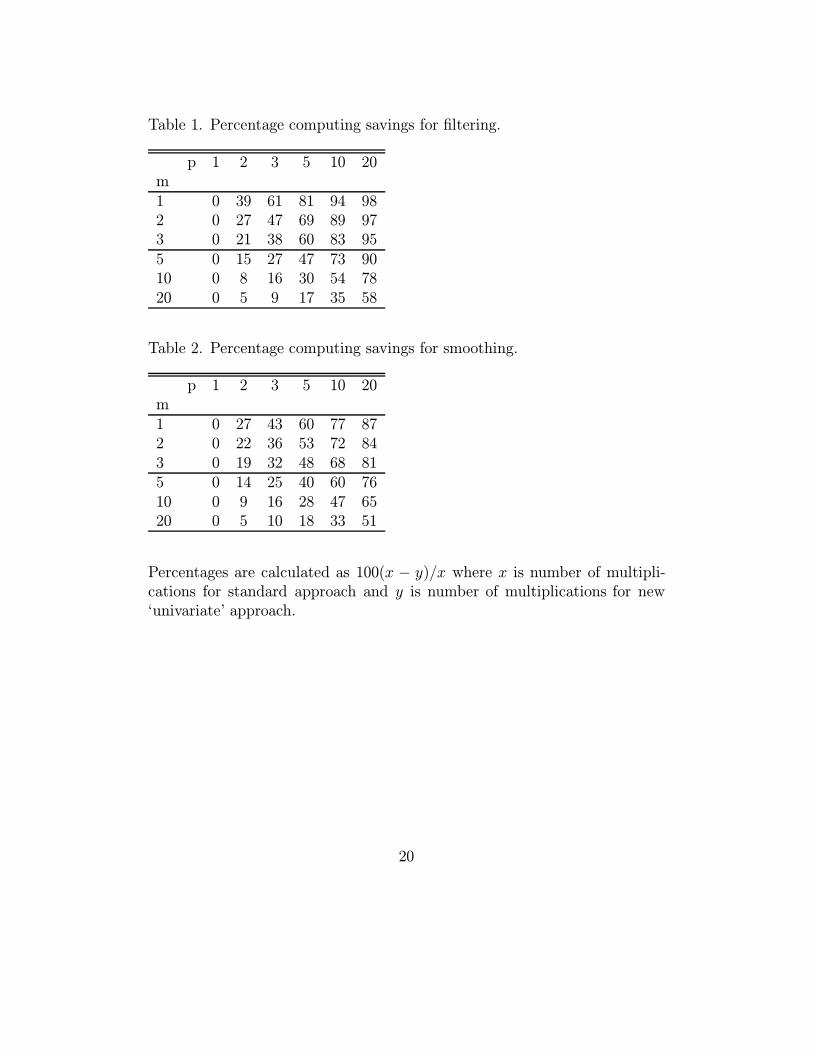
Table 1. Percentage computing savings for filtering.

p 1 2 3 5 10 20m1 0 39 61 81 94 982 0 27 47 69 89 973 0 21 38 60 83 955 0 15 27 47 73 9010 0 8 16 30 54 7820 0 5 9 17 35 58

Table 2. Percentage computing savings for smoothing.

p 1 2 3 5 10 20m1 0 27 43 60 77 872 0 22 36 53 72 843 0 19 32 48 68 815 0 14 25 40 60 7610 0 9 16 28 47 6520 0 5 10 18 33 51

Percentages are calculated as 100(x − y)/x where x is number of multipli-cations for standard approach and y is number of multiplications for new‘univariate’ approach.

20