Feature-preserving volume filtering

Joint EUROGRAPHICS - IEEE TCVG Symposium on Visualization (2002)D. Ebert, P. Brunet, I. Navazo (Editors)

Feature-Preserving Volume Filtering

László Neumann�, Balázs Csébfalvi

�, Ivan Viola

�, Matej Mlejnek

�, and Eduard Gröller

�

Vienna University of Technology, Austria, http://www.cg.tuwien.ac.at/home/

AbstractIn this paper a feature-preserving volume filtering method is presented. The basic idea is to minimize a three-component global error function penalizing the density and gradient errors and the curvature of the unknownfiltered function. The optimization problem leads to a large linear equation system defined by a sparse coefficientmatrix. We will show that such an equation system can be efficiently solved in frequency domain using fast Fouriertransformation (FFT). For the sake of clarity, first we illustrate our method on a 2D example which is a deditheringproblem. Afterwards the 3D extension is discussed in detail since we propose our method mainly for volumefiltering. We will show that the 3D version can be efficiently used for elimination of the typical staircase artifactsof direct volume rendering without losing fine details. Unlike local filtering techniques, our novel approach ensuresa global smoothing effect. Previous global 3D methods are restricted to binary volumes or segmented iso-surfacesand they are based on area minimization of one single reconstructed surface. In contrast, our method is a generalvolume-filtering technique, implicitly smoothing all the iso-surfaces at the same time. Although the strength of thepresented algorithm is demonstrated on a specific 2D and a specific 3D application, it is considered as a generalmathematical tool for processing images and volumes.

Categories and Subject Descriptors (according to ACM CCS): I.3.3 [Computer Graphics]: Feature-preservingsmoothing, derivative and gradient estimation, direct volume rendering, antialiasing, noise filtering.

1. Introduction

There are several research areas, like noise filtering of sig-nals, image processing, or direct volume rendering, wherethe input data is available as a continuous function sampledat regular or irregular grid points. It is a recurring problem,how to reconstruct the most important features of the orig-inal signal from the sampled values. For instance, after dis-cretization the exact derivatives are not available anymore,therefore they have to be estimated from the samples.

The traditional approach is convolution-based filtering.The support of the filter kernels used in image-processing orvolume-visualization practice is usually limited to a narrowneighborhood. An ideal but computationally impractical re-construction however would require convolution filters with

�[email protected]�[email protected]�[email protected]�[email protected]@cg.tuwien.ac.at

infinite support, like the Sinc filter for function reconstruc-tion. A consequence of the local support is for example thestaircase aliasing in direct volume rendering. Even if somelow-pass filtering is used it remedies the problem only lo-cally since the voxels far away from a given voxel do nothave an effect on its estimated gradient. The global influencecan be ensured using iterative methods but they are rathertime-consuming and restricted to binary volumes 11 12.

Our goal is to develop a global smoothing method, whereeach sample has an influence on all the others, but samplesfar away from each other interact only very slightly. We wantto obtain smooth homogeneous regions but also achieve apreservation of important features. Sharp edges of an imageor well defined iso-surfaces in a volumetric data set have tobe retained.

First our method is illustrated on a 2D example whichis a dedithering problem. Afterwards we discuss the 3Dextension and its major application field which is feature-preserving volume filtering. In Section 2 we overview theprevious work that has been done in 3D feature reconstruc-

c�

The Eurographics Association 2002.

Neumann et al. / Feature-Preserving Volume Filtering

tion. Section 3 presents in detail the mathematical back-ground of our new method. Section 4 discusses the 2D caseand its application in image processing. Section 5 describesthe extension to 3D volumes and the adaptation for directvolume rendering of binary and gray-scale data sets. In Sec-tion 6 the contribution of this paper is summarized.

2. Previous work

Function and derivative reconstruction from sampled val-ues is a fundamental problem in computer graphics. One re-search direction is interpolation oriented assuming that ac-curate samples are available. The Sinc and Cosc functionsare considered as ideal interpolation and derivative filters re-spectively 8 9. For a practical use of the Sinc filter window-ing is suggested 10. Möller et al. 1 give a survey of existingdigital derivative filters and compare their accuracy analyt-ically. These derivative reconstruction techniques based onwindowing are local methods as for practical reasons onlya limited number of neighboring samples are taken into ac-count.

Another approach for derivative reconstruction is approx-imation oriented. Here it is assumed that the sampled func-tion is noisy, which is typical when some real physical prop-erties are measured. The basic idea is to estimate the incli-nation or the normal from a larger neighborhood. In orderto reduce staircase aliasing several methods were proposedfor normal computation especially in binary volumes 2 3 4.Contextual shading techniques try to fit a locally approx-imating plane 5 or a biquadratic function 6 7 to the set ofpoints that belong to the same iso-surface. These methodsare time-consuming and limited to a certain neighborhood.Bryant and Krumvieda 5 solve a set of linear equations byGaussian elimination in order to obtain an approximate tan-gent plane at a given surface point. Webber’s technique 6 7

is similar to 5. In a 26-neighborhood the surface is approx-imated by a biquadratic function producing accurate resultsfor objects with C1 continuous faces. Neumann et al. 16 lin-early approximate the density function itself using a 3D re-gression hyperplane. Their approach leads to a computation-ally efficient convolution operation. The common drawbackof these approximation techniques is the local influence ofthe neighboring samples. It is rather easy to define cases,where staircase aliasing still appears in the generated imageeven if some more sophisticated local gradient estimation isapplied.

A rather new research direction is based on distance-transformation methods 11 14. Sramek 14 proposes a vox-elization method, where the generated volume contains den-sities proportional to the nearest distance from an analyti-cal surface. Smooth distance maps created also from binaryvolumes 13 can be exploited in gradient estimation. Gibson11 uses an iterative method based on this idea. Her “elas-tic surface net” creates a globally smooth surface modelfrom binary segmented volumes. Staircase artifacts can be

eliminated also using shape-based interpolation calculatingsmooth 2D distance maps 15. The main disadvantage of dis-tance transformation is its limitation to binary segmentedvolumes or to iso-surface-oriented applications.

Whitaker’s 12 approach is similar to Gibson’s 11 methodbut an iteration is performed directly on the volume withoutgenerating an intermediate triangular mesh. His technique isalso restricted to binary data sets.

In contrast, our method is a general tool for filtering bi-nary and gray scale volumes, making all the iso-surfacessmoother at the same time. Unlike convolution-based filter-ing, the smoothing effect is global due to a global curvatureminimization. Feature preservation is the main characteristicof our novel filtering approach. By globally penalizing largegradient deviations important features and fine details likeedges or iso-surfaces are preserved.

3. The new filtering algorithm

The input data is given as a noisy n-dimensional functionf sampled at regular grid points. We want to generate a fil-tered function f̃ with reduced noise and preserved features.The discrete samples are denoted by fi and f̃i respectively.We assume that the original function f contains continuousand smooth features as well as discontinuities. Our method isbased on a quadratic penalty function E. Given N samples fiwe are looking for N unknown samples f̃i which minimizethe penalty function. E is defined so that feature preserva-tion and smoothing is simultaneously possible. For reasonsof simplicity we illustrate the method first for the 1D case.Penalty function E consists of the following three compo-nents summed over every sample point i:

� difference squared between filtered value f̃i and originalvalue fi. This term ensures that the original values fi areclosely approximated by the filtered values f̃i.� difference squared between the gradients of the filteredvalue f̃i and the original value fi. This term ensures fea-ture preservation which means gradient preservation. Inareas of high gradient magnitude the gradient of filteredfunction f̃ must closely follow the gradient of f . Other-wise a large unwanted contribution to penalty functionE results. Filtered function f̃ will be a smooth functiontherefore central differences (

�f̃i � 1 � f̃i � 1 �� 2) are suffi-

cient to approximate the gradient of f̃ . This is not thecase for data values fi which might result from a binaryor noisy function f . Using central differences to estimatethe gradient of function f , would induce f̃ to follow stair-case or noise artifacts in f instead of approximating thetrue underlying gradient of f . The gradient at fi is there-fore approximated with gi which is calculated accordingto a more sophisticated gradient-estimation scheme (Ap-pendix 8.1.)16. The derivative function g is based on linearregression and contains only locally-reduced staircase ar-tifacts. Additionally the gradient differences between f̃i

c�



and fi are multiplied by a weighting factor G which de-termines the impact of feature preservation on the penaltyfunction E.� the squared curvature of the filtered function f̃ . To achievesmoothing we are looking for a function f̃ with smalloverall curvature. The curvature at point i is approximatedby the difference between the gradient at point i (approx-imated by f̃i � 1 � f̃i) and the gradient at point i � 1 (ap-proximated by f̃i � f̃i � 1). This term is multiplied by aweighting factor S which determines the importance ofsmoothing.

In the 1D case the penalty function E therefore has thefollowing structure (the second term is multiplied by 4 inorder to simplify the further mathematical derivation):

E � ∑i

� �f̃i � fi � 2 � (1)

4 � G � � � f̃i � 1 � f̃i � 1 �� 2 � gi � 2 �S � � f̃i � 1

� f̃i � 1 � 2 f̃i � 2 ��Using the above curvature and gradient estimation

schemes it is assumed that the values f̃i represent N num-ber of replicated samples in an infinite periodical signal,therefore f̃i

� f̃i � N . This assumption is necessary, since inour method, as it will be shown in the further discussion,a 3D Fourier transform of the original volume will be ex-ploited. Before we describe how to find filtered values f̃ithat minimize the global error we shortly discuss several de-grees of freedom in penalty function E. The weights S andG determine the relative importance of feature preservationas opposed to smoothing. The linear regression based gradi-ent estimation (function g) takes a local neighborhood intoaccount (Appendix 8.1.). Increasing the size of this neigh-borhood reduces local staircase artifacts but also increasessmoothing. Noise reduction can be achieved by omitting gra-dients below a certain threshold. In this case function f̃ doesnot try to follow small noise-related gradient variations inf . Instead of simple thresholding non-linear operations ongradient magnitudes of g are also possible. By, e.g., em-phasizing high gradient magnitudes, only the most impor-tant features are preserved. The minimization of the penaltyfunction E results in a globally smooth filtered function f̃preserving the fine details due to the gradient component.

Since we use non-negative G and S parameters thepenalty function E is a convex quadratic function having aunique global minimum. At the minimum location the par-tial derivatives according to all the N unknown values f̃i haveto be equal to zero, where i � 0 � 1 � 2 � � � � � N � 1:

∂E�f̃0 � f̃1 � f̃2 � � � � � f̃N � 1 �� ∂ f̃i

� 0 � (2)

As penalty function E is a quadratic function, the partialderivatives are linear functions of variables f̃i. Therefore,having all of these partial derivatives evaluated, a large linearequation system is obtained with N unknown variables:

A � f̃ � m � (3)

where A is a sparse coefficient matrix, and f̃ is the unknownvector containing the N samples of the filtered function. Vec-tor m is derived from the original function samples fi in thefollowing way:

mi� fi � 2G � � gi � 1 � gi � 1 � � (4)

Matrix A, derived from the partial derivatives, is definedby a symmetric point spread vector p:

p � �p1 � p2 � p3 � p4 � p5 � � �

S � G � � 4S � 1 � 6S � 2G � � 4S � S � G � �(5)

A ��

p3 p4 p5 0 � p1 p2p2 p3 p4 p5 � 0 p1p1 p2 p3 p4 � 0 00 p1 p2 p3 � p5 0� � � � � p4 p5p5 0 0 p1 p2 p3 p4p4 p5 0 0 p1 p2 p3

� ��

�

In 1D, the coefficient matrix A is a symmetric circular ma-trix. At first sight, it seems that the solution of the large equa-tion system (3) would require tremendous computationaltime. One possibility of optimization is to exploit the specialstructure of matrix A. Unfortunately, when the minimizationproblem is extended to 2D and 3D the coefficient matrix willnot have such a simple structure. In this case, the unknownvector f̃ contains all the pixels of the unknown image or allthe voxels of the unknown volume. The structure of the co-efficient matrix depends on the ordering of these elements.However, matrix A is always a symmetric positive definitematrix, therefore the inverse exists and it is also symmet-ric and positive definite. A linear equation system definedby such a coefficient matrix can be solved by applying theconjugated gradient method. According to our experience,in case of S � 50 and G � 50 this matrix was well condi-tioned ensuring the numerical stability of gradient methods.

As an alternative, we present a fast method for solving thelinear equation in frequency domain. In fact, function m iscalculated by a convolution of the unknown function f̃ withthe kernel p:

mi� 5

∑j � 1

f̃i � j � 3 � p j � (6)

c�



Here we assumed that f̃ � 1� f̃N � 1, f̃ � 2

� f̃N � 2, f̃N� f̃0,

and f̃N � 1� f̃1. Because of this assumption, there will be a

slight interaction between the opposite border regions of theoutput signal. This interaction can be reduced by adding anappropriately thick zero extension at the borders.

In the frequency domain the convolution operation is rep-resented by a multiplication: M

�ω � � F̃

�ω � � P �

ω � . There-fore, the Fourier transform F̃ of the unknown vector f̃ can becalculated as F̃

�ω � � M

�ω �� P

�ω � . In the spatial domain the

multiplication with matrix A is equivalent with a convolutionwith kernel p. Similarly, the multiplication with inverse ma-trix A � 1 is equivalent with a deconvolution with p, whichcan be written as a convolution with a kernel p

�

, which isthe inverse Fourier transform of P

� �ω � � 1 � P

�ω � . Such a

deconvolution operation in frequency domain is unambigu-ous (a division by zero problem does not occur) if there isa unique solution of the equivalent linear equation system,which means that matrix A is invertable.

This can be proven in the following way. Matrix A isderived from the partial derivatives of a convex (G andS are non-negative parameters) quadratic penalty function.The penalty function is formally the sum of N number of�aix

� bi � 2 terms, therefore the coefficient matrix A can bewritten as the sum of diadic products of the correspondingterms ai � aT

i . Since each term is positive semidefinite, ma-trix A is also positive semidefinite. It is easy to see that incase of non-negative G and S parameters the matrix A is notonly positive semidefinite but positive definite, and thereforeit is invertable.

Thus, the unknown function f̃ is calculated as an inverseFourier transform of F̃ . Using fast Fourier transformation(FFT) our filtering algorithm consists of the following steps:

1. estimation of gradients gi using linear regression2. non-linear operations on the gradient function g3. calculation of function m using the modified g4. M � FFT

�m � - Fourier transform of function m

5. P � FFT�p � - Fourier transform of function p

6. F̃ � M � P - deconvolution in frequency domain7. f̃ � INVFFT

�F̃ � - inverse Fourier transform of F̃

The second step is optional and can be an arbitrary non-linear operation on the gradient function g. The 2D and 3Dextension of our method requires 2D and 3D kernel p and m.The derivation is analogous to the 1D case. Results for p andm are given in Appendix 8.2.

4. 2D application - Dedithering

In the image-processing literature there are various lo-cal edge-preserving smoothing methods. Global techniques,which are similar to our approach, like the snake (active con-tours) 17 19 18 method or the total variation 20 21 method alsominimize a global penalty function in order to reduce noiseand enhance contours. The first and second order derivative

terms used by these methods are fundamentally differentfrom the schemes of our method. The global error is min-imized applying different iterative techniques, and usuallythe numerical stability requires an appropriate precondition-ing. In contrast, our method does not rely on an iterativesolution and does not use any additional (for example La-grange) constraints, therefore it is fast and numerically sta-ble.

In order to make the volume smoothing application moreunderstandable, we illustrate our filtering algorithm on a 2Dexample which is a dedithering problem. A binary ditheredimage can be considered as a noisy representation of theoriginal image with significant loss of information. Theproblem is how to reconstruct the original features like sharpedges, smooth homogeneous regions, and fine details fromthe binary pixels of the dithered image.

In the 2D penalty function the gradients g�i � j � are esti-

mated using linear regression (Appendix 8.1.). In the secondterm of the penalty function (weighted by G) the gradientsof the unknown image are defined by central differences:

f̃x�i � j � � �

f̃�i � 1 � j � � f̃

�i � 1 � j � � � 2 � (7)

f̃y�i � j � � �

f̃�i � j � 1 � � f̃

�i � j � 1 � � � 2 �

In the third term of the penalty function (weighted by S)we use the following quadratic norm of the Hessian matrixas a measure of the local curvature:

f̃ 2xx

� f̃ 2yy

� 2 f̃ 2xy � (8)

The 2D algorithm is analogous to the 1D case. The con-stant term m in Equation 3 and the convolution kernel p(defining the coefficient matrix A) are derived from theEquations 2. The result of the derivation is presented in Ap-pendix 8.2.

We illustrate the 2D version of our filtering method ona binary dithered image. A low resolution detail of this isshown in Figure 1a. For the sake of comparison, first we triedto apply a Gaussian filter to generate a gray-scale image ap-proximating the original one. We used a rather narrow kernel(σ � 1 � 5) in order to smooth the homogeneous regions with-out removing the fine details. Figure 1b shows the result ofthe Gaussian filtering.

Figure 1c shows an image generated applying our feature-preserving filtering. We used parameter settings G � 10 andS � 24. Note that, compared to the Gaussian filtering thehigh frequency details are well preserved. There are alsosome clearly visible details which are hardly recognizableeven by the human eyes when you take a look at the ditheredimage in Figure 1a.

c�



(a) (b) (c)

Figure 1: (a) The original binary dithered image. (b) Gaussian filtering. (c) Feature-preserving filtering.

(a) (b) (c)

Figure 2: The middle slice of the equivalent convolution kernel p�

using varying parameter settings: (a) S = 0, G = 1, (b) S =1, G = 1, (c) S = 1, G = 0.

5. 3D application - Volume filtering

In this section we discuss how to extend our method to the3D case and how to apply it for feature-preserving volumefiltering. Each gradient value g

�i � j � k � is estimated using lin-

ear regression (Appendix 8.1.).

In the 3D penalty function E the gradients in the filteredvolume are approximated by central differences. The gradi-ent component of E (weighted by G) is extended to 3D asfollows:

G � � � f̃x�i � j � k � � gx

�i � j � k �� 2 � (9)

�f̃y

�i � j � k � � gy

�i � j � k �� 2 �

�f̃z�i � j � k � � gz

�i � j � k �� 2 ��

The curvature term of E (weighted by S) can be extendedto 3D using finite differences to approximate the followingformula:

f̃ 2xx

� f̃ 2yy

� f̃ 2zz

� (10)

2 � f̃ 2xy

� 2 � f̃ 2xz

� 2 � f̃ 2yz �

Note that, the derived linear equation system (3) containsas many unknown variables as the number of voxels which is2563 for a typical data set. Fortunately, due to the deconvolu-tion performed in frequency domain, the optimization prob-lem can be efficiently solved. The 3D filtering algorithm isanalogous to the 1D case. Appendix 8.2. presents the derivedconstant term m of Equation 3 and the 3D kernel p used forthe deconvolution in Step 6.

In order to illustrate the global behavior of our method wecalculated the equivalent convolution kernels which have tobe applied for the modified volume m to obtain the same re-sults. The Fourier transform P

�

of the equivalent kernel p�

contains the reciprocals of the coefficients in P. Therefore,kernel p

�

can be easily calculated as the inverse transform ofP

�

. Figure 2 shows the middle slice of p�

evaluated for vary-ing S and G parameters and rendered as gray-scale images.The filter values are non-linearly overemphasized in orderto visualize also the low weights. Note that, if weight G isdominant then the kernel is similar to a Gaussian filter whilesetting a dominant S weight the kernel is getting similar to aSinc function. In fact, the images in Figure 2 depicting con-volution kernels in the spatial domain, represent the inverse

c�



of the coefficient matrix A in Equation 3. Such an equivalentconvolution kernel exists if a non-linear operation in the 2.step of the algorithm is not applied. Since this is a crucialstep of the algorithm, in general it is not possible to substi-tute our method with a simple convolution-based filtering.

Parameter S controls the smoothing of iso-surfaces andparameter G is responsible for preserving the fine detailsin the volume. Figure 3 shows a very low-resolution (64 �

64 � 32) artificial binary volume which contains several dis-cretized objects. This binary data set was filtered using vary-ing S and G parameters. The higher the parameter G is,the better the estimated gradients g

�i � j � k � are approximated.

Since linear regression using a larger voxel neighborhood re-sults in a smooth gradient function an increased G has alsoa local smoothing effect. This effect is controlled by the ra-dius r of the considered neighborhood and the sphericallysymmetric weighting function. Here the gradients g

�i � j � k �

were estimated from a 26-neighborhood weighted by 1 � d3 ,where d is the Euclidean distance of a neighboring voxelfrom the current voxel. In a special case gradient estimationbased on linear regression provides the same results as cen-tral differences, making the local smoothing effect minimal(Appendix 8.1.). Gradients approximated from such a nar-row voxel neighborhood are preferred when also voxel-sizedetails are required to be preserved.

Increasing parameter S the global smoothing effect is get-ting stronger because of the weighted curvature minimiza-tion. In case of G � 0 and S �� 0 the results approximateonly very roughly the original surfaces, and small details areremoved. This can be compensated by setting a higher valueof G. Figure 3 illustrates how these contradictory conditionsfight each other. Generally, the appropriate parameter settingis always a compromise, depending on whether one wants toemphasize small details or rather to enhance smooth charac-teristic surfaces.

For the sake of comparison, Figure 4 shows the renderingof the original binary volume (a) and the filtered volume (b).In order to make the surfaces smoother and to preserve thesmall details at the same time, we used parameters G � 3and S � 3.

Figure 5 shows a gray-scale data set of a lobster filteredusing varying S and G parameters. Figure 6 compares theimages of the original and the filtered data generated with thesame rendering conditions. For the filtering, we used S � 3and G � 12 in order to preserve small details like the feelerof the lobster.

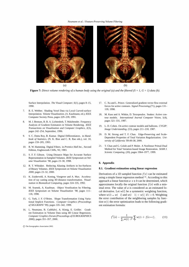
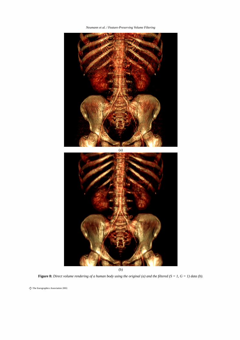
We tested our method also using a more complex trans-fer function emphasizing two different density ranges at thesame time. Figure 7 (see color section) shows the renderingof a human body using the original CT data set (a) and the fil-tered volume (b). The test data set is rather noisy and it con-tains contrast material in the blood vessels having nearly thesame densities as the bone. Therefore, an appropriate trans-fer function has to be very fine tuned in order to render the

vessels separately from the bone. Figure 7a shows an imagerendered using the original data set. Note that, the final im-age contains point like noise and typical staircase artifacts. Inorder to remedy these problems we filtered the volume withparameters G � 1 and S � 1. We also applied a thresholdcutting according to the gradient magnitudes for noise re-duction. The entire filtering process took 8 minutes for sucha 202 � 152 � 255 resolution volume on an 800 MHz Pen-tium PC with 512M RAM. Figure 7b shows the visualizationof the filtered volume using the same rendering parametersas for the original data. Note that the details are well pre-served and the iso-surfaces are much smoother. The pointlike noise is also significantly reduced.

Figure 7 also illustrates that our method is basicallya volume-filtering method making all the iso-surfacessmoother inside the volume and it is not restricted to onesingle iso-surface like the previous global smoothing tech-niques.

6. Conclusion

In this paper a feature-preserving volume filtering methodhas been presented. With a three-component penalty func-tion, approximation of the original values, feature preser-vation and curvature minimization can be controlled effi-ciently. Images generated by direct volume rendering fromthe filtered data contain only reduced point like noise andstaircase artifacts. Furthermore, the sampled smooth sur-faces and fine details can be reconstructed at the sametime. Unlike local convolution-based filtering techniques,our method provides a global smoothing effect because ofthe global curvature minimization. The scalability is ensuredby the weighting parameters of the three-component penaltyfunction. Due to the applied FFT method filtering is per-formed efficiently. Our approach is not restricted to binarydata or segmented iso-surfaces, unlike previous techniquesbased on iterative solution. Although the presented filteringalgorithm has been illustrated on a specific 2D and a spe-cific 3D example it can be considered as a general math-ematical tool usable for image or volume-processing pur-poses. Among the possible 2D application fields we mentionfeature-preserving smoothing or zooming, image restora-tion, and terrain-modeling. In the 3D case, our technique isapplicable to gradient-driven or shape-based interpolation,and smoothing of binary segmented masks.

7. Acknowledgements

The work presented in this publication has been fundedby the ADAPT project (FFF-804544). ADAPT is supportedby Tiani Medgraph, Vienna (http://www.tiani.com), andthe Forschungsförderungsfonds für gewerbliche Wirtschaft,Austria. See http://www.cg.tuwien.ac.at/research/vis/adaptfor further information on this project. Special thanks toTorsten Möller and Attila Neumann for their useful com-ments.

c�



S = 3 S = 6 S = 12

G = 0

G = 3

Figure 3: A binary volume filtered with varying S and G parameters.

(a) (b)

Figure 4: Rendering of a 64 � 64 � 32 binary volume using the original (a) and the filtered (S = 3, G = 3) data (b).

References

1. T. Möller, R. Machiraju, K. Müller, R. Yagel. A Comparisionof Normal Estimation Schemes. Proceedings of IEEE Visual-ization ’97, pages 19–26, 1997.

2. G. Thürmer, C. A. Wüthrich. Normal Computation for Dis-crete Surfaces in 3D Space. Computer Graphics Forum (Pro-ceedings of EUROGRAPHICS ’97), pages 15–26, 1997.

3. R. Yagel, D. Cohen, A. Kaufman. Normal Estimation in 3D

c�



S = 3 S = 6 S = 12

G = 0

G = 3

Figure 5: A CT scan of a lobster filtered with varying S and G parameters.

(a) (b)

Figure 6: Rendering of the lobster using the original (a) and the filtered (S = 3, G = 12) data (b).

Discrete Space. The Visual Computer, 8, pages 278–291,1992.

4. D. Cohen, A. Kaufman, R. Bakalash, S. Bergman. Real TimeDiscrete Shading. The Visual Computer, 6, pages 16–27, 1990.

5. J. Bryant, C. Krumvieda. Display of 3D Binary Objects: I-shading. Computers and Graphics, 13(4), pages 441–444,1989.

6. R. E. Webber. Ray Tracing Voxel Data via Biquadratic Local

c�



(a) (b)

Figure 7: Direct volume rendering of a human body using the original (a) and the filtered (S = 1, G = 1) data (b).

Surface Interpolation. The Visual Computer, 6(1), pages 8–15,1990.

7. R. E. Webber. Shading Voxel Data via Local Curved-surfaceInterpolation. Volume Visualization, (A. Kaufmann, ed.), IEEEComputer Society Press, pages 229–239, 1991.

8. M. J. Bentum, B. B. A. Lichtenbelt, T. Malzbender. FrequencyAnalysis of Gradient Estimators in Volume Rendering. IEEETransactions on Visualization and Computer Graphics, 2(3),pages 242–254, September, 1996.

9. S. C. Dutta Roy, B. Kumar. Digital Differentiators. in Hand-book of Statistics, (N. K. Bise and C. R. Rao eds.), vol. 10,pages 159–205, 1993.

10. R. W. Hamming. Digital Filters. in Prentice Hall Inc., SecondEdition, Englewoods Cliffs, NJ, 1983.

11. S. F. F. Gibson. Using Distance Maps for Accurate SurfaceRepresentation in Sampled Volumes. IEEE Symposium on Vol-ume Visualization ’98, pages 23–30, 1998.

12. R. T. Whitaker. Reducing Aliasing Artifacts in Iso-Surfacesof Binary Volumes. IEEE Symposium on Volume Visualization2000, pages 23–32, 2000.

13. K. Zuiderveld, A. Koning, Viergever and A. Max. Accelera-tion of ray casting using 3D distance transformation. Visual-ization in Biomedical Computing, pages 324–335, 1992.

14. M. Sramek, A. Kaufman. Object Voxelization by Filtering.IEEE Symposium on Volume Visualization ’98, pages 111–118, 1998.

15. G. Turk, J. F. O’Brien. Shape Transformation Using Varia-tional Implicit Functions. Computer Graphics (Proceedingsof SIGGRAPH ’99), pages 335–342, 1999.

16. L. Neumann, B. Csébfalvi, A. König, E. Gröller. Gradi-ent Estimation in Volume Data using 4D Linear Regression.Computer Graphics Forum (Proceedings of EUROGRAPHICS2000), pages 351–357, 2000.

17. C. Xu and L. Prince. Generalized gradient vector flow externalforces for active contours. Signal Processing,(71), pages 131–139, 1998.

18. M. Kass and A. Witkin, D. Terzopoulos. Snakes: Active con-tour models. International Journal Computer Vision, 1(4),pages 321–331, 1987.

19. L. D. Cohen. On active contour models and balloons. CVGIP:Image Understanding, (53), pages 211–218, 1987.

20. D. M. Strong and T. F. Chan. Edge-Preserving and Scale-Dependent Properties of Total Variation Regularization. Uni-versity of California TR-00-38, 2000.

21. T. Chan and G. Golub and P. Mulet. A Nonlinear Primal-DualMethod for Total Variation-based Image Restoration. SIAM J.Scientic Computing, (20), pages 1964–1977, 1999.

8. Appendix

8.1. Gradient estimation using linear regression

Derivatives of a 1D sampled function f�x � can be estimated

using a simple linear regression method 16. According to thisapproach a linear function a � x � b can be determined, whichapproximates locally the original function f

�x � with a min-

imal error. The value of a is considered as an estimated lo-cal derivative. Let w

�i � be a symmetric weighting function,

where w�i � � w

� � i � and w�i � 1 � � w

�i � if i � 0. Weighting

the error contribution of the neighboring samples by func-tion w

�i � the error optimization leads to the following gradi-

ent estimation formula:

f� �

x � � 1

∑i w�i � � i2 ∑

iw�i � � i � f

�x � i � � (11)

c�



This method can be easily extended to 2D and 3D gra-dient estimation. In 2D, denoting the sampled function asf�x � y � and the symmetric weighting function as w

�i � j � the

estimated gradient components are calculated the followingway:

fx�x � y � � 1

∑i � j w�i � j � � i2 ∑

i � j w�i � j � � i � f

�x � i � y � j � � (12)

fy�x � y � � 1

∑i � j w�i � j � � j2 ∑

i � j w�i � j � � j � f

�x � i � y � j � �

where w�i � j � � w

� � i � � j � and w�i � j � � w

�k � l � if i2 � j2 �

k2 � l2.

The 3D gradient estimation formulas are analogous to the2D case:

fx�x � y � z � � 1

W � i2 ∑i � j � k w

�i � j � k � � i � f

�x � i � y � j � z � k � � (13)

fy�x � y � z � � 1

W � j2 ∑i � j � k w

�i � j � k � � j � f

�x � i � y � j � z � k � �

fz�x � y � z � � 1

W � k2 ∑i � j � k w

�i � j � k � � k � f

�x � i � y � j � z � k � �

where W � ∑i � j � k w�i � j � k � . In fact, these gradient estimation

schemes define kernels for computationally efficient convo-lution. The convolution is evaluated only for those neigh-boring samples, where the weighting function w is greaterthan zero. The weighting function controls the smoothnessof the estimated gradient function. The wider the consideredneighborhood is the stronger is the local smoothing effect.For instance, in 3D the classical gradient estimation basedon central differences is a special case of the linear regres-sion method using the following weighting function:

w�i � j � k � �

�� 1 if i �� 1 � � 1 � � j � 0 � k � 0or i � 0 � j �� 1 � � 1 � � k � 0or i � 0 � j � 0 � k �� 1 � � 1 �

0 otherwise.

(14)

In this special case the local smoothing is minimal since justa narrow voxel neighborhood is taken into account.

8.2. The 2D and 3D convolution kernels

In the 2D case, the convolution kernel p derived from Equa-tions 2 is defined as the following 5 � 5 point spread matrix:

p ��

S8 0 3

4 S � G 0 S8

0 0 � 4S 0 034 S � G � 4S 1 � 4G � 12 � 5S � 4S 3

4 S � G0 0 � 4S 0 0S8 0 3

4 S � G 0 S8

� ��

The 2D function m�i � j � in Equation 3 is calculated simi-

larly to the 1D case:

m�i � j � � f

�i � j � � (15)

2G � � � gx�i � 1 � j � � gx

�i � 1 � j � �

gy�i � j � 1 � � gy

�i � j � 1 � ��

In the 3D case, the derived convolution kernel p is a 5 �

5 � 5 volume. Let us denote the ith slice by pi. Because ofthe symmetric kernel p1

� p5 and p2� p4. The slices are

defined by the following matrices:

p1�

�

0 0 S8 0 0

0 0 0 0 0S8 0 S

2 � G 0 S8

0 0 0 0 00 0 S

8 0 0

� ��

p2�

�

0 0 0 0 00 0 0 0 00 0 � 4S 0 00 0 0 0 00 0 0 0 0

� ��

p3�

�

S8 0 S

2 � G 0 S8

0 0 � 4S 0 0S2 � G � 4S 1 � 6G � 19 � 5S � 4S S

2 � G0 0 � 4S 0 0S8 0 S

2 � G 0 S8

� ��

The constant term m�i � j � k � in Equation 3 is analogous to

the 2D case:

m�i � j � k � � f

�i � j � k � � (16)

2G � � � gx�i � 1 � j � k � � gx

�i � 1 � j � k � �

gy�i � j � 1 � k � � gy

�i � j � 1 � k � �

gz�i � j � k � 1 � � gz

�i � j � k � 1 � ��

c�



(a)

(b)

Figure 8: Direct volume rendering of a human body using the original (a) and the filtered (S = 1, G = 1) data (b).

c�


Feature-preserving volume filtering

Documents

Transcript of Feature-preserving volume filtering