Privacy-Preserving Location-based Services

Privacy-Preserving Location-based Services

A DISSERTATION

SUBMITTED TO THE FACULTY OF THE GRADUATE SCHOOL

OF THE UNIVERSITY OF MINNESOTA

BY

Chi Yin Chow

IN PARTIAL FULFILLMENT OF THE REQUIREMENTS

FOR THE DEGREE OF

Doctor Of Philosophy

May, 2010

Acknowledgements

First and foremost, I would like to express my deepest gratitude to my advisors Dr.

Mohamed F. Mokbel and Dr. Tian He. Especially, it has been an honor to be Dr.

Mokbel’s first Ph.D. student. They have taught me how high quality computer science

research is done. I appreciate all their contributions of time, ideas, guidance, and funding

to make my Ph.D. experience productive and stimulating. The joy and enthusiasm they

have for their research was motivational for me, even during tough times in the Ph.D.

pursuit. I am also thankful for the excellent example they have provided as a successful

scholar and professor.

The members of the Data Management Lab, Jie Bao, Biplob Debnath, Abdeltawab

Hendawi, Mohamed Khalefa, Justin Levandoski, Joe Naps, and Mohamed Sarwat, and

the members of the Sensor System Group, Yu Gu, Shuo Guo, Jaehoon Jeong, Qingquan

Zhang, Ziguo Zhong, and Ting Zhu, and other peers, Rene Bustamante, Colin DeLong,

David Kuo-Wei Hsu, Taehyun Hwang, James Kang, Gaurav Pandey, Nishith Pathak,

and Daniel Sandler, have contributed immensely to my personal and professional time

at Minnesota. These people have been a source of friendships as well as good advice

and collaboration.

I would also like to thank Dr. Xuan Liu, the mentor of my summer intern at

the IBM Thomas J. Watson Research Center in 2008, and other great collaborators,

Prof. Walid G. Aref (Purdue University), Dr. Jinchuan Chen (Renmin University),

Dr. Reynold Cheng (The University of Hong Kong ), Dr. Hong-Va Leong (The Hong

Kong Polytechnic University), and Dr. Suman Nath (Microsoft Research) for giving

their insight suggestions to my research and sharing their research experiences and

knowledge with me.

i

For this thesis, I would like to thank my final oral examination committee mem-

bers, Prof. Shashi Shekhar (the chair) and Dr. Gediminas Adomavicius (the external

member), for their time, insight questions, and helpful comments.

Last but not the least, I would like to thank my fiancee Christine Liu, my sister

Aster Chow, and my parents for all their endless love, support, and encouragement.

This thesis is dedicated to all of them.

ii

Dedication

To my fiancee Christine Liu, my sister Aster Chow, and my parents.

iii

ABSTRACT

Location-based services (LBS for short) providers require users’ current locations to

answer their location-based queries, e.g., range and nearest-neighbor queries. Revealing

personal location information to potentially untrusted service providers could create

privacy risks for users. To this end, our objective is to design a privacy-preserving

framework for LBS where users can obtain LBS and preserve their location privacy. In

this thesis, we propose privacy-preserving LBS frameworks for different environments:

(1) client-server environments in Euclidean space (the Casper system), (2) client-server

environments in road networks, (3) mobile peer-to-peer environments, and (4) location

monitoring services in wireless sensor networks (the TinyCasper system). In general,

these frameworks have two main modules, namely, location anonymization and privacy-

aware query processing. The location anonymization module blurs an user’s exact loca-

tion into a cloaked area (or a cloaked road segment set in road network environments)

that satisfies the user’s privacy requirements. The proposed frameworks support the

two most popular privacy requirements, k-anonymity, i.e., a user is indistinguishable

among k users, and minimum area Amin (or minimum total length of a cloaked road

segment set), i.e., the size of a cloaked area is at least Amin. The user is able to specify

his/her privacy requirements in a privacy profile and change the privacy profile at any

time. The privacy-aware query processing module is embedded inside a database server

to provide LBS based on cloaked areas (or cloaked road segment sets). To prove the

concept of our privacy-preserving LBS frameworks, we implement system prototypes for

Casper and TinyCasper. For each proposed privacy-preserving LBS framework, we con-

duct extensive experiments to evaluate the performance of its location anonymization

and privacy-aware query processing modules. All experiment results show that the pro-

posed frameworks are scalable and efficient with respect to large numbers of users, large

numbers of queries, and various privacy requirements, and they provide high quality

services in terms of the accuracy of query answers and the query response time.

iv

Contents

Acknowledgements i

Dedication iii

Abstract iv

List of Tables ix

List of Figures x

1 Introduction 1

1.1 Related Work . . . . . . . . . . . . . . . . . . . . . . . . . . . . . . . . . 5

1.1.1 Location Privacy . . . . . . . . . . . . . . . . . . . . . . . . . . . 5

1.1.2 Location-based Query Processing . . . . . . . . . . . . . . . . . . 6

1.1.3 Privacy Models . . . . . . . . . . . . . . . . . . . . . . . . . . . . 7

1.1.4 Privacy-Aware Query Processing . . . . . . . . . . . . . . . . . . 7

1.2 Organization of the Thesis . . . . . . . . . . . . . . . . . . . . . . . . . . 8

2 The Casper System 10

2.1 Architecture . . . . . . . . . . . . . . . . . . . . . . . . . . . . . . . . . . 11

2.2 System Prototype . . . . . . . . . . . . . . . . . . . . . . . . . . . . . . . 12

3 Location Anonymization in Casper 16

3.1 The Basic Location Anonymizer . . . . . . . . . . . . . . . . . . . . . . 17

3.2 The Adaptive Location Anonymizer . . . . . . . . . . . . . . . . . . . . 19

3.3 Discussion . . . . . . . . . . . . . . . . . . . . . . . . . . . . . . . . . . . 21

v

3.4 Experiment Results . . . . . . . . . . . . . . . . . . . . . . . . . . . . . . 22

3.4.1 The Pyramid Height . . . . . . . . . . . . . . . . . . . . . . . . . 23

3.4.2 Scalability . . . . . . . . . . . . . . . . . . . . . . . . . . . . . . . 25

3.4.3 Effect of Privacy Profile . . . . . . . . . . . . . . . . . . . . . . . 26

3.5 Summary . . . . . . . . . . . . . . . . . . . . . . . . . . . . . . . . . . . 27

4 Query Processing in Casper 28

4.1 Snapshot Privacy-Aware Query Processing . . . . . . . . . . . . . . . . . 29

4.1.1 Private Queries over Public Data . . . . . . . . . . . . . . . . . . 30

4.1.2 Public Queries over Private Data . . . . . . . . . . . . . . . . . . 39

4.1.3 Private Queries over Private Data . . . . . . . . . . . . . . . . . 41

4.2 Continuous Privacy-aware Query Processing . . . . . . . . . . . . . . . . 47

4.2.1 Basic Continuous Privacy-aware Query Processing . . . . . . . . 48

4.2.2 Shared Execution Paradigm for Continuous Privacy-aware Query

Processing . . . . . . . . . . . . . . . . . . . . . . . . . . . . . . . 50


4.3.1 Effect of Performance Tuning Parameters . . . . . . . . . . . . . 63

4.3.2 Scalability . . . . . . . . . . . . . . . . . . . . . . . . . . . . . . . 68

4.3.3 Effect of Privacy Requirements . . . . . . . . . . . . . . . . . . . 71

4.4 Summary . . . . . . . . . . . . . . . . . . . . . . . . . . . . . . . . . . . 72

5 Approximate Range Nearest Neighbor Queries 73

5.1 System Model . . . . . . . . . . . . . . . . . . . . . . . . . . . . . . . . . 76

5.2 Approximate Range NN Query Processing . . . . . . . . . . . . . . . . . 78

5.2.1 Building Voronoi Diagrams . . . . . . . . . . . . . . . . . . . . . 78

5.2.2 Access Method for Voronoi Diagrams . . . . . . . . . . . . . . . 78

5.2.3 Online Query Processing Algorithm . . . . . . . . . . . . . . . . 81

5.3 Experimental Results . . . . . . . . . . . . . . . . . . . . . . . . . . . . . 85

5.3.1 Effect of Approximation Tolerance Levels . . . . . . . . . . . . . 86

5.3.2 Effect of Query Region Size . . . . . . . . . . . . . . . . . . . . . 88

5.3.3 Effect of Number of Objects . . . . . . . . . . . . . . . . . . . . . 89

5.3.4 Effect of Object Size . . . . . . . . . . . . . . . . . . . . . . . . . 90

5.3.5 Effect of Communication Bandwidth . . . . . . . . . . . . . . . . 90

vi

5.4 Summary . . . . . . . . . . . . . . . . . . . . . . . . . . . . . . . . . . . 92

6 Query-Aware Location Anonymization in Road Networks 94

6.1 System Model . . . . . . . . . . . . . . . . . . . . . . . . . . . . . . . . . 96

6.2 Cost Model for Private Queries . . . . . . . . . . . . . . . . . . . . . . . 98

6.2.1 Private K-Nearest-Neighbor Queries . . . . . . . . . . . . . . . . 98

6.2.2 Private Range Queries . . . . . . . . . . . . . . . . . . . . . . . . 100

6.3 Query-Aware Anonymization . . . . . . . . . . . . . . . . . . . . . . . . 101

6.3.1 Motivation: A Trade-off between Query Cost and Query Quality 102

6.3.2 Objective Cost Function . . . . . . . . . . . . . . . . . . . . . . . 103

6.3.3 Greedy Approaches . . . . . . . . . . . . . . . . . . . . . . . . . . 104

6.4 Shared Execution Paradigm . . . . . . . . . . . . . . . . . . . . . . . . . 109

6.4.1 Motivation . . . . . . . . . . . . . . . . . . . . . . . . . . . . . . 110

6.4.2 Algorithm . . . . . . . . . . . . . . . . . . . . . . . . . . . . . . . 112


6.5.1 Scalability . . . . . . . . . . . . . . . . . . . . . . . . . . . . . . . 116

6.5.2 Privacy Requirements . . . . . . . . . . . . . . . . . . . . . . . . 117

6.5.3 Query Parameters . . . . . . . . . . . . . . . . . . . . . . . . . . 118

6.5.4 Randomness Factor . . . . . . . . . . . . . . . . . . . . . . . . . 119

6.5.5 Objective Cost Function . . . . . . . . . . . . . . . . . . . . . . . 120

6.5.6 Shared Execution Paradigm . . . . . . . . . . . . . . . . . . . . . 121

6.6 Summary . . . . . . . . . . . . . . . . . . . . . . . . . . . . . . . . . . . 124

7 Location Anonymization in Peer-to-Peer Environments 125

7.1 System Model . . . . . . . . . . . . . . . . . . . . . . . . . . . . . . . . . 127

7.2 Peer-to-Peer Spatial Cloaking Algorithm . . . . . . . . . . . . . . . . . . 130

7.2.1 Spatial Cloaking Algorithm . . . . . . . . . . . . . . . . . . . . . 130

7.2.2 Information Sharing Scheme . . . . . . . . . . . . . . . . . . . . . 134

7.2.3 Peer-to-Peer Spatial Cloaking in a Partitioned Network . . . . . 136

7.2.4 Cloaked Area Adjustment Scheme . . . . . . . . . . . . . . . . . 140

7.3 Anonymous Location-based Services . . . . . . . . . . . . . . . . . . . . 143


7.4.1 Anonymization Strength . . . . . . . . . . . . . . . . . . . . . . . 145

vii

7.4.2 Scalability . . . . . . . . . . . . . . . . . . . . . . . . . . . . . . . 146


7.4.4 Effect of Transmission Range . . . . . . . . . . . . . . . . . . . . 152

7.4.5 Effect of Uncertainty Tolerance . . . . . . . . . . . . . . . . . . . 152

7.5 Summary . . . . . . . . . . . . . . . . . . . . . . . . . . . . . . . . . . . 154

8 The TinyCasper System 156

8.1 System Model . . . . . . . . . . . . . . . . . . . . . . . . . . . . . . . . . 159

8.2 System Prototype . . . . . . . . . . . . . . . . . . . . . . . . . . . . . . . 162

9 Location Anonymization and Query Processing in TinyCasper 165

9.1 Location Anonymization Algorithms . . . . . . . . . . . . . . . . . . . . 166

9.1.1 The Resource-Aware Algorithm . . . . . . . . . . . . . . . . . . . 166

9.1.2 The Quality-Aware Algorithm . . . . . . . . . . . . . . . . . . . 170

9.2 Spatial Histogram . . . . . . . . . . . . . . . . . . . . . . . . . . . . . . 179

9.3 System Evaluation . . . . . . . . . . . . . . . . . . . . . . . . . . . . . . 181

9.3.1 Attacker Model . . . . . . . . . . . . . . . . . . . . . . . . . . . . 182

9.3.2 Simulation Settings . . . . . . . . . . . . . . . . . . . . . . . . . . 183

9.3.3 Performance Metrics . . . . . . . . . . . . . . . . . . . . . . . . . 184

9.4 Experimental Results and Analysis . . . . . . . . . . . . . . . . . . . . . 185

9.4.1 Anonymization Strength . . . . . . . . . . . . . . . . . . . . . . . 185

9.4.2 Effect of Query Region Size . . . . . . . . . . . . . . . . . . . . . 186

9.4.3 Effect of the Number of Objects . . . . . . . . . . . . . . . . . . 188


9.4.5 Effect of Mobility Speeds . . . . . . . . . . . . . . . . . . . . . . 190

9.5 Summary . . . . . . . . . . . . . . . . . . . . . . . . . . . . . . . . . . . 191

10 Conclusion and Discussion 192

10.1 Future Research Directions . . . . . . . . . . . . . . . . . . . . . . . . . 194

References 196

viii

List of Tables

4.1 The computational cost of each privacy-aware query type. . . . . . . . . 53

4.2 Summary of parameter settings. . . . . . . . . . . . . . . . . . . . . . . . 63

5.1 Parameter settings. . . . . . . . . . . . . . . . . . . . . . . . . . . . . . . 86


7.1 Summary of the features of our algorithms. . . . . . . . . . . . . . . . . 144



ix

List of Figures

2.1 The Casper system architecture. . . . . . . . . . . . . . . . . . . . . . . 11

2.2 The client GUI. . . . . . . . . . . . . . . . . . . . . . . . . . . . . . . . . 13

2.3 The basic location anonymizer. . . . . . . . . . . . . . . . . . . . . . . . 14

2.4 The adaptive location anonymizer. . . . . . . . . . . . . . . . . . . . . . 15

2.5 The server GUI. . . . . . . . . . . . . . . . . . . . . . . . . . . . . . . . 15

3.1 The basic location anonymizer. . . . . . . . . . . . . . . . . . . . . . . . 17

3.2 The adaptive location anonymizer. . . . . . . . . . . . . . . . . . . . . . 20

3.3 Map of Hennepin County, MN, USA. . . . . . . . . . . . . . . . . . . . . 23

3.4 Effect of the pyramid structure height for the location anonymizer. . . . 24

3.5 Effect of the number of users for the location anonymizer. . . . . . . . . 25

3.6 Effect of the k-anonymity levels for the location anonymizer. . . . . . . 26

4.1 Two trivial approaches for processing private queries over public data. . 30

4.2 Example of a private nearest-neighbor query over public data (refine = 1). 34

4.3 Two termination cases for the query processing of private queries over

public data. . . . . . . . . . . . . . . . . . . . . . . . . . . . . . . . . . . 37

4.4 Example of a public nearest-neighbor query over private data. . . . . . . 40

4.5 Example of a private nearest-neighbor query over private data (refine = 1). 43

4.6 Some termination cases for private queries over private data. . . . . . . 46

4.7 The effect of δ for the shared execution paradigm. . . . . . . . . . . . . 52

4.8 Example of the shared execution paradigm for a private continuous

nearest-neighbor query over public data (refine = 1). . . . . . . . . . . . 55

4.9 refine values (private queries over public data). . . . . . . . . . . . . . . 64

4.10 refine values (private queries over private data). . . . . . . . . . . . . . . 64

4.11 Number of static query points (private queries over public data). . . . . 65

x

4.12 Number of static query points (public queries over private data). . . . . 66

4.13 Number of static query points (private queries over private data). . . . . 66

4.14 δ values (private queries over public data). . . . . . . . . . . . . . . . . . 67

4.15 δ values (public queries over private data). . . . . . . . . . . . . . . . . . 67

4.16 δ values (private queries over private data). . . . . . . . . . . . . . . . . 68

4.17 Number of users (private queries over public data). . . . . . . . . . . . . 68

4.18 Number of users (private queries over private data). . . . . . . . . . . . 69

4.19 Number of data (private queries over public data). . . . . . . . . . . . . 69

4.20 Number of data (private queries over private data). . . . . . . . . . . . . 70

4.21 Data object size (total processing time). . . . . . . . . . . . . . . . . . . 70

4.22 k-anonymity requirements (private queries over public data). . . . . . . 71

4.23 k-anonymity requirements (private queries over private data). . . . . . . 71

5.1 A motivating example for approximate range NN queries. . . . . . . . . 75

5.2 The 1-order and 2-order Voronoi diagrams for five sites s1 to s5. . . . . 77

5.3 The base level of an incomplete pyramid structure. . . . . . . . . . . . . 79

5.4 Incomplete pyramid structure. . . . . . . . . . . . . . . . . . . . . . . . 80

5.5 Range NN query processing using Voronoi diagrams. . . . . . . . . . . . 81

5.6 Example of a range search in the incomplete pyramid structure (Figure 5.4). 82

5.7 Inverted lists. . . . . . . . . . . . . . . . . . . . . . . . . . . . . . . . . . 84

5.8 Example of the query-covering step, based on Figure 5.7b. . . . . . . . . 85

5.9 Approximation tolerance levels (t). . . . . . . . . . . . . . . . . . . . . . 87

5.10 Query region size. . . . . . . . . . . . . . . . . . . . . . . . . . . . . . . 88

5.11 Number of objects. . . . . . . . . . . . . . . . . . . . . . . . . . . . . . . 89

5.12 Object size. . . . . . . . . . . . . . . . . . . . . . . . . . . . . . . . . . . 90

5.13 Downlink bandwidth at vehicular speeds (128 kbps). . . . . . . . . . . . 91

5.14 Downlink bandwidth at stationary or very slow speeds (2 Mbps). . . . . 92

6.1 Spatial cloaking for the Euclidean space. . . . . . . . . . . . . . . . . . . 95

6.2 Private K-nearest-neighbor query. . . . . . . . . . . . . . . . . . . . . . . 100

6.3 A trade-off between query quality and cost. . . . . . . . . . . . . . . . . 102

6.4 Example of the greedy approach. . . . . . . . . . . . . . . . . . . . . . . 107

6.5 Motivating example of shared execution. . . . . . . . . . . . . . . . . . . 110

xi

6.6 An example of the shared execution scheme for a query set Q =

{Q1, Q2, Q3}. . . . . . . . . . . . . . . . . . . . . . . . . . . . . . . . . . 112

6.7 Number of mobile users (K-NN queries). . . . . . . . . . . . . . . . . . . 116

6.8 k-anonymity (K-NN queries). . . . . . . . . . . . . . . . . . . . . . . . . 117

6.9 Minimum length Lmin (K-NN queries). . . . . . . . . . . . . . . . . . . . 118

6.10 Query parameters. . . . . . . . . . . . . . . . . . . . . . . . . . . . . . . 119

6.11 Random factor RandF (K-NN queries). . . . . . . . . . . . . . . . . . . 119

6.12 Objective cost function (K-NN queries). . . . . . . . . . . . . . . . . . . 120

6.13 Number of queries. . . . . . . . . . . . . . . . . . . . . . . . . . . . . . . 121

6.14 Privacy requirements (K-NN queries). . . . . . . . . . . . . . . . . . . . 122

6.15 Query parameters. . . . . . . . . . . . . . . . . . . . . . . . . . . . . . . 123

7.1 System architecture. . . . . . . . . . . . . . . . . . . . . . . . . . . . . . 127

7.2 Example of the peer-to-peer spatial cloaking algorithm. . . . . . . . . . 132

7.3 Example of peer-to-peer spatial cloaking in a partitioned network. . . . 139

7.4 Examples of the cloaked area adjustment scheme. . . . . . . . . . . . . . 142

7.5 Privacy-aware nearest-neighbor query processing. . . . . . . . . . . . . . 143

7.6 “Center-of-cloaked-area” privacy attack. . . . . . . . . . . . . . . . . . . 147

7.7 Number of querying users. . . . . . . . . . . . . . . . . . . . . . . . . . . 148

7.8 Number of users. . . . . . . . . . . . . . . . . . . . . . . . . . . . . . . . 149

7.9 Number of data objects. . . . . . . . . . . . . . . . . . . . . . . . . . . . 150

7.10 k-anonymity privacy requirements. . . . . . . . . . . . . . . . . . . . . . 151

7.11 Minimum area privacy requirements. . . . . . . . . . . . . . . . . . . . . 152

7.12 Transmission range. . . . . . . . . . . . . . . . . . . . . . . . . . . . . . 153

7.13 Uncertainty tolerance for the information sharing scheme (tols). . . . . . 154

8.1 A location monitoring system using counting sensors. . . . . . . . . . . . 157

8.2 System architecture. . . . . . . . . . . . . . . . . . . . . . . . . . . . . . 159

8.3 The prototype of TinyCasper on a physical test-bed with 39 MICAz motes.161

8.4 Server GUI - aggregate locations reported from sensor nodes. . . . . . . 162

8.5 Server GUI - a spatial histogram and range queries. . . . . . . . . . . . 163

9.1 System overview. . . . . . . . . . . . . . . . . . . . . . . . . . . . . . . . 166

9.2 The resource-aware location anonymization algorithm (k = 5). . . . . . 167

9.3 The search space S of sensor node A. . . . . . . . . . . . . . . . . . . . . 171

xii

9.4 The lattice structure of a set of four items. . . . . . . . . . . . . . . . . 174

9.5 The quality-aware cloaked area of sensor node A. . . . . . . . . . . . . . 175

9.6 Example of histogram maintenance. . . . . . . . . . . . . . . . . . . . . 181

9.7 Attacker model error. . . . . . . . . . . . . . . . . . . . . . . . . . . . . 185

9.8 Query region size. . . . . . . . . . . . . . . . . . . . . . . . . . . . . . . 186

9.9 Number of objects. . . . . . . . . . . . . . . . . . . . . . . . . . . . . . . 187

9.10 Anonymity levels. . . . . . . . . . . . . . . . . . . . . . . . . . . . . . . . 188

9.11 Object mobility speeds. . . . . . . . . . . . . . . . . . . . . . . . . . . . 190

xiii

Chapter 1

Introduction

Location-based services (LBS) combine the functionality of location-aware devices (e.g.,

GPS-like devices), wireless communication technologies, and information management

to provide personalized services for users based on their current locations. Examples

of LBS include location-aware emergency services, e.g., “Dispatch the nearest ambu-

lance”, location-based advertisement, e.g., “Send e-coupons to all cars that are within

two miles of my gas station”, live traffic reports, e.g., “What is shortest path from my

current location to a destination”, and location-based store finders, e.g., “Where is my

nearest restaurant”. The user registered with LBS continuously send his/her location

to a location-based database server. Upon requesting LBS, the registered user issues

a location-based query that is executed at the server based on the knowledge of the

user’s current location [1, 2, 3, 4]. Location-based queries can be categorized into either

snapshot or continuous queries. Examples of snapshot queries include “Where is my

nearest gas station” and “What are the restaurants within one mile of my location”,

while examples of continuous queries include “Continuously report my nearest police

car” and “Continuously report the gas stations within one mile of my car”.

Although LBS promise safety and convenience, they threaten the privacy and se-

curity of their users. The privacy threat comes from the fact that LBS providers rely

mainly on an implicit assumption that the user agrees to reveal his/her private location

to get LBS. In other words, the user trades his/her privacy with the service. If the

user wants to keep his/her private location information, the user has to turn off the

location-aware device and (temporarily) unsubscribe from the service. With potentially

1

2

untrusted servers, such a service subscription model poses several privacy threats to the

user. For example, an employer may check on his/her employee’s behavior by knowing

the places where the employee visits and the time of each visit, the personal medical

records can be inferred by knowing which clinic a person visits, or someone can track

the locations of his/her ex-friends. In many real-life cases, people abuse GPS devices to

stalk personal locations [5, 6, 7], and many people worry about their location privacy

when they are using LBS [8]. Unfortunately, the traditional approach of pseudonymity

(i.e., using a fake identity) [9] is not applicable to LBS, as the location information of

a person can directly lead to the true identity. For example, asking about the nearest

Pizza restaurant to the location of my house using a fake identity will reveal my true

identity, as a resident of the house. In fact, many web-based tools are available to

translate a location into a street address (e.g., Google Maps [10]) and find the resident

of a street address (e.g., Intelius [11]).

In this thesis, we first present the Casper system [12, 13]; a query processing frame-

work for privacy-preserving LBS. Casper consists of two main components, location

anonymizer and privacy-aware query processor. The location anonymizer, which is a

trusted third party placed between the user and the database server, blurs a user’s

exact location point into a cloaked area that satisfies the user’s privacy requirements.

Casper supports the two most popular privacy requirements, k-anonymity, i.e., a user is

indistinguishable among k users, and minimum area Amin. Thus, a user’s cloaked area

contains at least k− 1 other users and the size of the cloaked area is at least Amin. The

privacy-aware query processor is embedded inside the database server to process both

snapshot and continuous location-based queries based on cloaked areas rather than lo-

cation points. The privacy-aware query processor supports three types of privacy-aware

queries: (1) private queries over public data, (2) public queries over private data, and

(3) private queries over private data. Data and/or queries are public if their exact

location information is reported to the database server, while data and/or queries are

private if only their cloaked location areas are reported to the database server. Since

the privacy-aware query processor only knows that the query issuer and/or data are

located in cloaked areas, the query processor can only returns a candidate answer set

to the location anonymizer. Casper guarantees that the candidate answer set includes

the exact answer to the user. As the location anonymizer knows the exact location of

3

the query issuer and data, it computes the exact answer for the user. To prove the con-

cept of Casper, we implement a system prototype for Casper [14], where the location

anonymizer is implemented as a stand-alone server placed between the user and the

database server, and the privacy-aware query processor is implemented as query oper-

ators inside the PLACE server; a scalable location-aware database server developed by

the Purdue University for spatio-temporal data streams [15, 16].

In some other privacy-preserving LBS frameworks, the user has to blur his/her

location into a cloaked area without the help of the location anonymizer and contact

the database server directly. Thus, the user has to receive the entire candidate answer

set from the database server, and then computes the exact answers from the candidate

answer set. Since the bandwidth of communication channels between the mobile user

and the database server could be very limited (e.g., the downlink bandwidth of 3G

mobile subscribers ranges from 128 kbps at vehicular speeds to 2 Mbps at stationary or

very slow speeds), we propose an approximate range nearest-neighbor query, i.e., private

queries over public data, with a quality guarantee [17]. It is important to note that the

proposed query processing algorithm can also be used to deal with uncertain locations,

where the user’s location is modeled as a spatial area to capture its uncertainty. Given

a query region and an approximation tolerance level t, the query processing algorithm

returns a candidate answer set such that at least one of the t nearest objects of every

point inside the query region is in the candidate answer set. The larger the value of t,

the smaller the candidate answer set is returned to the user from the database server.

Thus, the approximation tolerance level t can be served as a tuning parameter that

trades off between the query response time and the quality of answers.

We extend the functionalities of Casper to road network environments [18], where a

user’s location is blurred into a set of connected road segments rather than a spatial area.

Each user specifies two privacy parameters k and Lmin in his/her privacy profile, such

that the user’s cloaked segment set contains at least k users and the total length of the

cloaked segment set is at least Lmin. The extended query processing framework is not

only designed specifically for the road network environment, but it is also “query-aware”

as it aims to balance between the query execution cost and the size of the candidate

answer set returned to the user from the database server.

In mobile peer-to-peer (P2P) networks, where mobile users can only communicate

4

with other peers through multi-hop routing without any support of fixed communication

infrastructure or centralized/distributed servers. The mobile P2P networks have many

unique limitations, e.g., user mobility, limited transmission range, multi-hop communi-

cation, scarce communication resources, and network partitions1 . With the advances

in wireless communication technologies and mobile devices, the mobile P2P networks

have become an important computing platform, so we propose a P2P spatial cloaking

algorithm that mainly extends the functionality of the location anonymizer of Casper to

the mobile P2P networks [19, 20]. The main idea of the P2P spatial cloaking algorithm

is that when a mobile user wants to obtain services from an LBS provider, the user

collaborates with other peers via multi-hop communication to blur his/her location into

a cloaked area. Our algorithm guarantees that the cloaked area satisfies the user’s k-

anonymity and minimum area Amin privacy requirements. Then, the user sends his/her

location-based query along with the cloaked area to the database server. After the user

gets the candidate answer set from the database server, the user computes the exact

answer from the candidate answer set.

This thesis finally presents the TinyCasper system; a privacy-preserving location

monitoring system designed for wireless sensor networks [21]. In traditional location

monitoring systems, sensors are deployed in the system to track personal locations. How-

ever, monitoring personal locations with a potentially untrusted system poses privacy

threats to the monitored individuals, because an adversary could abuse the location in-

formation gathered by the system to infer personal sensitive information [22, 23, 24, 25].

To tackle the privacy breach in location monitoring systems, each sensor node blurs its

sensing area into a cloaked area, in which at least k persons are residing. TinyCasper

only allows each sensor node to report aggregate location information, which is in a

form of a cloaked area along with the number of persons, N , located in the cloaked

area, where N ≥ k, to the server. It is important to note that the value of k achieves

a trade-off between the strictness of privacy protection and the accuracy of monitoring

services. A smaller k indicates less privacy protection, because a smaller cloaked area

will be reported from the sensor node to the server; hence, more accurate monitoring

services. However, a larger k results in a larger cloaked area, which will reduce the

1 In a partitioned network, mobile users are partitioned into disjoint networks, in which a mobileuser is only able to communicate with other peers residing in his/her network partition.

5

accuracy of monitoring services, but it provides better privacy protection. Although

TinyCasper only knows the aggregate location information about the monitored per-

sons, it can still provide monitoring services through answering aggregate queries, for

example, “What is the number of persons in a certain area”. To support aggregate

queries, we propose a spatial histogram that analyzes the aggregate locations reported

from the sensor nodes to estimate the distribution of the monitored persons in the sys-

tem. The estimated distribution is used to answer the aggregate queries. To prove the

concept of TinyCasper, we implement a system prototype for TinyCasper [26] with 39

MICAz motes [27] on a physical test-bed, and the spatial histogram is implemented

inside the base station computer with visualization.

1.1 Related Work

In this section, we highlight the related work to privacy-preserving LBS in four different

areas, namely, location privacy, location-based query processing, privacy models, and

privacy-aware query processing.

1.1.1 Location Privacy

Motivated by the privacy threats of location-detection devices [28, 29, 30, 31], recent

attempts for providing location privacy in location-based services (LBS) (e.g., [32, 30,

19, 33, 34, 35, 36, 37, 38, 39, 40, 41, 42, 43, 44, 45, 46, 47, 48]) and other location-aware

applications (e.g., context-aware computing [49] and sensor networks [23]) focus only

on the location anonymizer part. Although such techniques would be valuable for pro-

tecting users’ private locations in LBS, the practicality in real location-based database

servers is doubtful as these techniques lack privacy-aware query processing capacity.

By protecting users’ location information from being disclosed to the location-based

database server, processing these location privacy-preserving queries becomes challeng-

ing where new techniques need to be presented to provide efficient query processing

while not being able to know users’ exact locations.

In general, four different approaches have been explored: (1) False dummies [45]. For

every location update, a user sends n different locations to the server with only one of

them is true while the rest are dummies. Thus, the server cannot know which one of these

6

locations is the actual one. (2) Landmark objects [43]. Rather than sending the exact

location to a location-based database server, the user refers to the location of a certain

landmark or a significant object. (3) Location perturbation [32, 19, 33, 34, 35, 36, 37, 38,

39, 40, 41, 44, 46, 47, 48]. The main idea is to blur a user’s exact location into a cloaked

area using either spatial or temporal cloaking [32, 19, 33, 36, 37, 38, 39, 41, 44, 46, 47, 48]

or location obfuscation [35]. The cloaked area can be based either on the k-anonymity

concept [50, 51, 52] (i.e., the area should contain at least k users) or on a graph model

that represents a road network [35]. (4) Avoid location tracking [30, 40]. While the

previous three approaches focus only on hiding a certain instance of the user location,

this approach aims to avoid tracking the user behavior.

Among these location anonymization techniques, our proposed privacy-aware query

processor supports the location perturbation techniques that blur users’ exact locations

into rectilinear areas, i.e., cloaked areas, as this is the most commonly used form of

location anonymization in many various environment settings, e.g., [32, 19, 36, 37, 38,

39, 41, 44] for snapshot locations, [33, 34, 47, 48] for continuous locations, [48] for spatial

networks, and [26, 23] for wireless sensor networks.

1.1.2 Location-based Query Processing

A plethora of techniques has been proposed to deal with various snapshot location-based

queries (e.g., [53, 54, 55, 56, 57, 58, 59]) and continuous location-based queries (e.g., [60,

61, 62, 63, 64, 3, 65, 66]). The main idea of snapshot queries is to provide an efficient and

real-time execution of location-based queries using spatio-temporal index structures for

frequently updated data. On the other hand, query processors for continuous location-

based queries have mainly focused on efficiency and scalability. In terms of efficiency,

several techniques have been proposed to use grid-based structures to support location-

based services for moving data and moving queries (e.g., [61, 62, 3, 67, 65]). In terms

of scalability, several techniques have proposed to employ a shared execution paradigm

in which multiple concurrent continuous queries can be evaluated simultaneously at

the location-based database server (e.g., [68, 60, 65, 69]). However, all these query

processors for snapshot and continuous location-based queries rely on the knowledge

of the users’ exact locations as none of these techniques have considered private data

and/or private queries.

7

1.1.3 Privacy Models

During the last decade, several paradigms of architecture have been explored to provide

secure data transformation from the client to the server machines. Secure-multi-party

communication [70, 71] organizes the communication among m parties such that each

party can have the knowledge of only a certain function but not the actual data for

other parties. However, the computational overhead of such a scheme prevents its direct

application to database problems. Thus, the minimal information sharing [72] paradigm

is proposed where it uses cryptographic techniques to perform join and intersection

operations. However, the computational cost and the inability to serve other queries

make such a paradigm not suitable for real time applications. The untrustworthy third

party [73] paradigm has been proposed in the context of peer-to-peer systems. The main

idea is to employ a third party that executes queries by collecting secure information

from multiple data sources, i.e., peers. The most commonly used model is the trusted

third party [74, 75] paradigm. The main idea is to employ a third party that is trusted

by the users and acts as a middle layer between the user and the database server.

Among these models, our framework employs the trusted third party model as it

requires less computational overhead and is more suitable for real-time query processing.

The trusted third party model is already utilized by existing location privacy techniques

(e.g., [30, 32, 19, 33, 36, 37, 41, 44, 46, 12, 47, 48]) and is commercially applied in

other fields. For example, the Anonymizer [76] is for anonymous web surfing while the

PayPal [77] system is a trusted third party where a user can buy products without

giving his/her credit card information to the provider.

1.1.4 Privacy-Aware Query Processing

Recent research efforts have been dedicated to deal with location privacy-preserving

queries, i.e., getting anonymous services from location-based applications (e.g., [34, 78,

44, 79, 80, 12, 81]). These query processing frameworks can be divided into three main

categories. (1) Location obstruction [81]. The basic idea is that a querying user first

sends a query along with a false location to a database server, and the database server

keeps sending the list of nearest objects to the reported false location to his/her until the

list of received objects satisfies the user’s privacy and quality requirements. (2) Space

8

transformation [78, 79]. This approach converts the original location of data and queries

into another space through a trusted third party. The space transformation maintains

the spatial relationship among the data and query, in order to provide accurate query

answers. (3) Cloaked area processing [34, 44, 80, 12]. In this framework, a privacy-aware

query processor is embedded in the database server side to deal with the cloaked spatial

area received either from a querying user [34, 80] or from a trusted third party [44, 12].

Among the existing cloaked area processing frameworks, the works [80, 44] are closest

to ours. These works find the exact set of objects as a query answer based on the linear

nearest neighbor search algorithm [82]. The difference between these two works is that

the work [80] considers rectilinear cloaked areas while the other one considers circular

cloaked areas [44]. The key distinctions between these two works and our proposed

privacy-aware query processor are follows: (1) Our query processor has the ability to

ease the optimality of query answers by finding a superset of the minimal answer set

that contains the exact answer, in order to achieve system scalability. We use a tuning

parameter to trade off between the system scalability and the candidate answer set

size. (2) According to our classification of privacy-aware queries, these two previous

works consider only private queries over public data, so they cannot be applied to the

case of private data. (3) We consider continuous privacy-aware queries by proposing a

shared execution paradigm that aims to improve system scalability when dealing with a

numerous number of privacy-aware continuous queries. The shared execution paradigm

also provides two other tuning parameters to trade off between system scalability and

answer optimality. The detail of our privacy-aware query processor will be described in

Section 4.

1.2 Organization of the Thesis

In this chapter, we have described the background of privacy-preserving LBS and the

motivation and contribution of this thesis. The rest of this thesis is organized as follows:

• Chapter 2 describes the architecture and system model of the Casper system, and

the Casper prototype.

• Chapter 3 presents the location anonymization algorithms used by the location

9

anonymizer of Casper to blur users’ locations into cloaked areas.

• Chapter 4 gives the query processing algorithms proposed for the privacy-aware

query processor of Casper to process the three introduced privacy-aware query

types, i.e., private queries over public data, public queries over private data, and

private queries over private data.

• Chapter 5 presents the query processing algorithm for approximate range nearest-

neighbor queries with quality guarantees.

• Chapter 6 describes the query-aware location anonymization algorithms and query

processing algorithms for privacy-preserving LBS in road network environments.

• Chapter 7 gives the spatial cloaking algorithm, designed for location anonymiza-

tion, in mobile P2P environments.

• Chapter 8 describes the architecture and system model of the TinyCasper system,

and the TinyCasper prototype.

• Chapter 9 presents the in-network location anonymization algorithms and the

spatial histogram, designed for supporting aggregate query processing, in Tiny-

Casper.

• Chapter 10 concludes this thesis and discusses future research directions in

privacy-preserving LBS.

Chapter 2

The Casper System

This chapter describes the architecture of the Casper system and the Casper prototype.

In Casper, mobile users can entertain location-based services (LBS) without the need

to reveal their private location information. Upon registration with Casper, the mobile

users specify their desired level of privacy through a user privacy profile. A user privacy

profile includes two parameters k and Amin. k indicates that the mobile user wants to

be k-anonymous, i.e., not distinguishable among other k users while Amin indicates that

the user wants to hide her location information within an area of at least Amin. Large

values for k and Amin indicate stricter privacy requirements. Our employed privacy

profile matches the privacy requirements of mobiles users as depicted by several social

science studies (e.g., see [29, 40, 42, 83, 84]).

Casper mainly consists of two components, namely, the location anonymizer and the

privacy-aware query processor. The location anonymizer is a trusted third party that

acts as a middle layer between the mobile user and the location-based database server

in order to: (1) receive the user’s exact location along with his/her privacy profile,

(2) blur the user’s exact location into a cloaked area based on the user’s privacy profile,

and (3) send the cloaked area to the location-based database server. The privacy-

aware query processor is embedded inside the location-based database server to tune its

functionality to deal with anonymous queries and cloaked areas rather than the exact

location information. We identify three novel query types that are supported by Casper:

(a) Private queries over public data, e.g., “Where is my nearest gas station”, in which

the person who issues the query is a private entity while the data (i.e., gas stations) are

10

11

��

��

��

��

��

��

��

��

��

��

��

�� !�"��

��

#��

��

Figure 2.1: The Casper system architecture.

public, (b) Public queries over private data, e.g., “How many cars in a certain area”,

in which a public entity asks about personal private locations, and (c) Private queries

over private data, e.g., “Where is my nearest buddy” in which both the person who

issues the query and the requested data are private. With this classification in mind,

traditional location-based query processors can support only public queries over public

data. Due to the lack of the exact location information at the server, the privacy-aware

query processor returns a candidate answer set instead of a single exact answer to the

location anonymizer. Since the location anonymizer knows the user’s exact location,

it computes the exact answer for the user. In Chapter 4, we prove that the candidate

answer set returned by our privacy-aware query processor is inclusive, i.e., the candidate

answer set contains the exact answer to the user, and is minimal, i.e., the candidate

answer set size is minimal.

2.1 Architecture

Figure 2.1 depicts the system architecture of Casper, which has two main compo-

nents: the location anonymizer and the privacy-aware query processor. The location

anonymizer receives location updates from mobile users, blurs their locations to cloaked

areas that match their user privacy profiles (k,Amin), and sends the cloaked areas to

the location-based database server. While cloaking the user’s location information, the

location anonymizer also removes any user identity from the user’s request to ensure the

pseudonymity of the location information [9]. Similar to the exact point locations, the

location anonymizer also blurs the query location information before sending a cloaked

query area to the location-based database server.

The privacy-aware query processor is embedded inside the location-based database

12

server to deal with location-based queries based on cloaked areas rather than exact

location points. Instead of returning an exact answer, the privacy-aware query processor

returns a candidate answer set for the location-based query to the location anonymizer.

As the location anonymizer knows the user’s exact location, it computes the exact

answer for the user. The privacy-aware query processor guarantees that the candidate

answer set contains the exact query answer. The size of the candidate list heavily

depends on the user privacy profile. A stricter privacy profile would result in a larger

candidate list. With user privacy profiles, mobile users have the ability to adjust a

personal trade-off between the amount of information they would like to reveal about

their locations and the size of the candidate answer sets that they obtain from Casper.

Location-based queries processed at the privacy-aware location-based database server

may be received either from the mobile users or from public administrators. Queries

that come from mobile users are considered as private queries and should pass by the

location anonymizer to hide the query identity and blur the location of the user who

issues the query. Location-based queries that are issued from public administrators are

considered as public queries and do not need to pass through the location anonymizer,

instead, they are directly submitted to the location-based database server. The database

server will answer such public queries based on the stored blurred location information

of all mobile users.

2.2 System Prototype

The system prototype of Casper consists of three different modules that can run on three

different machines, namely, the client module (Figure 2.2), the location anonymizer mod-

ule (Figures 2.3 and 2.4), and the location-based database server module (Figure 2.5).

While both the client and the location anonymizer are implemented as stand alone ap-

plications, the privacy-aware query processor is implemented as query operators inside

the PLACE server; a research prototype for location-based database services [2, 15].

Figure 2 gives a GUI screen shot of the client module. The GUI is divided into four

parts: (1) A road network map that displays the position of the client roaming on the

road network. In addition, query results that are requested by the client are displayed

on the road network map. (2) The privacy profile interface where the user can update

13

Figure 2.2: The client GUI.

the values of k and Amin at any time and submit the updated privacy profile to the

location anonymizer. (3) The query submission interface in which the client has the

ability to choose from four different query types, public query over public data, private

query over public data, public query over private data, and private query over private

data. Notice that the first query type is the traditional query type in location-based

database servers while the latter three query types are unique to Casper. With each

query type, there is a set of controls that appears to the clients to help in forming the

required query without actually writing the SQL query. Figure 2.2 gives an example

where the client selects a private query over public data. In this case, the client has the

ability to choose either a range query or a nearest-neighbor query. In case of a range

query, the client has to specify the range around its location. The SQL query will be

displayed to the user for illustration. (4) The query result interface in which the query

answer is tabulated to the user in addition to being shown on the road network map.

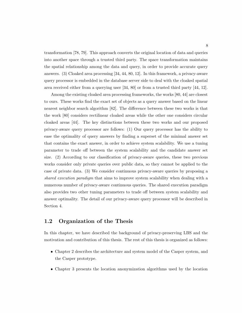
Figures 2.3 and 2.4 give the GUI screen shot for the basic and adaptive location

anonymizers, respectively. The details of the basic and adaptive location anonymizers

are described in Chapter 3. The GUI mainly shows the current exact locations of

all participating mobile users over the road network. The level of the pyramid data

structure is displayed as a grid over the road network. The number of mobile users at

14

Figure 2.3: The basic location anonymizer.

each grid cell is displayed along with the grid level in the case of the adaptive anonymizer

(Figure 2.4). As a default, the GUI displays only the lowest-level maintained cells.

As a result, all grid cells in the basic location anonymizer GUI are of the same size

(Figure 2.3) while in the adaptive location anonymizer GUI, grid cells have different

sizes (Figure 2.4). For illustration, there is a set of controls at the top of the GUI for

both location anonymizers that: (1) Alternates the GUI to show either the basic or the

adaptive location anonymizer, (2) Controls the maximum level of the pyramid structure,

(3) Turns on/off the counter display at each grid cell, and (4) Sets a parameter that

refreshes the GUI every certain milliseconds in order to achieve better visualization.

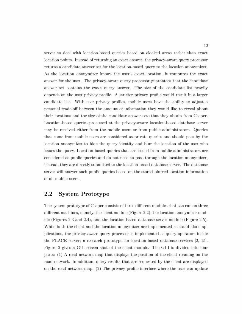
Figure 2.5 gives the GUI screen shot for the privacy-aware location-based database

server which is implemented inside the PLACE server [2, 15]. The GUI shows the road

network map with the exact locations of stationary public data (e.g., restaurants, gas

stations, and hospitals) and moving public data (e.g., police cars). For private data (i.e.,

user location information), the server can show only the cloaked area that is received

from the location anonymizer. The query processing steps are shown on the server

console during the query life time.

15

Figure 2.4: The adaptive location anonymizer.

Figure 2.5: The server GUI.

Chapter 3

Location Anonymization in

Casper

In this chapter, we describe the data structures designed for the location anonymizer

in Casper. As depicted in Figure 2.1 (in Chapter 2), the location anonymizer blurs the

exact location point of each mobile user to a cloaked area R that satisfies each user’s

privacy profile. To avoid the drawbacks of previous location anonymizers [85, 37], i.e.,

the assumption of a system-wide static k-anonymity for all users [37] and the support of

only small k-anonymity levels (k ≈ 10) [85], we identify the following four requirements

that we aim to satisfy in our location anonymizer:

1. Accuracy. The cloaked area R should be of area AR and contain kR users that

satisfy and as close as possible to the user profile (i.e., kR & k, AR & Amin).

2. Quality. An adversary can only know that the exact user location information

could be equally likely anywhere within the cloaked area R.

3. Efficiency. The cloaking algorithm should be computationally efficient and scal-

able. It should be able to cope with the continuous movement of large numbers

of mobile users and real-time requirements of spatio-temporal queries.

4. Flexibility. Each registered user with the location anonymizer should have (1) the

ability to specify her own privacy requirements and (2) the ability to change her

requirements at any time.

16

17

��

��

��

��

��

��

��

��

��

��

��

��

��

��

��!��"#

��!��$#

��!��#

��!��%#

Figure 3.1: The basic location anonymizer.

Notice that the spatio-temporal cloaking algorithm in [37] can support only the

quality requirement, while the CliqueCloak algorithm in [85] can partially support the

accuracy and flexibility requirements in terms of the k-anonymity parameter. In the

rest of this section, we present two alternative techniques for our location anonymizer

that satisfy the above four requirements, namely, the basic location anonymizer and the

adaptive location anonymizer.

3.1 The Basic Location Anonymizer

Data structure. Figure 3.1 depicts the data structure for the basic location

anonymizer. The main idea is to employ a grid-based complete pyramid data struc-

ture [86] that hierarchically decomposes the spatial space into H levels where a level of

height h has 4h grid cells. The root of the pyramid is of height zero and has only one

grid cell that covers the whole space. Each pyramid cell is represented as (cid,N) where

cid is the cell identifier while N is the number of mobile users within the cell boundaries.

The pyramid structure is dynamically maintained to keep track of the current number

of mobile users within each cell. In addition, we keep track of a hash table that has one

entry for each registered mobile user with the form (uid, profile, cid) where uid is the

mobile user identifier, profile is the user’s privacy profile, and cid is the cell identifier

in which the mobile user is located. cid is always at the lowest level of the pyramid (the

shaded level in Figure 3.1).

18

Algorithm 1 Bottom-up Cloaking Algorithm

1: Function BottomUp-Cloaking(k,Amin, cid)2: if cid.N ≥ k and cid.Area ≥ Amin then3: return Area(cid);4: end if5: cidV ← The vertical neighbor cell of cid.6: cidH ← The horizontal neighbor cell of cid.7: NV = cid.N + cidV .N , NH = cid.N + cidH .N8: if (NV ≥ k OR NH ≥ k) AND 2cid.Area ≥ Amin then9: if (NH ≥ k AND NV ≥ k AND NH ≤ NV ) OR NV < k then

10: return Area(cid) ∪Area(cidH);11: else12: return Area(cid) ∪Area(cidV );13: end if14: else15: BottomUp-Cloaking((k,Amin),Parent(cid));16: end if

Maintenance. Due to the highly dynamic environment of location-based appli-

cations, any employed data structure should be sustainable to frequent updates. A

location update is sent to the location anonymizer in the form (uid, x, y) where uid is

the user identifier, x and y are the spatial coordinates of the user’s new location. Once

the update is received at the location anonymizer, a hash function h(x, y) is applied to

get the user cell identifier cidnew at the lowest grid layer. Then, the user entry in the

hash table is checked to get its original cell identifier cidold. If the old cell identifier

matches the new one (cidold = cidnew), then there is no need to do any more processing.

If there is a change in the cell identifier (cidold 6= cidnew), three operations should take

place: (1) Update the new cell identifier in the hash table, (2) Update the counters N

in both the old and new pyramid grid cells, and (3) If necessary, propagate the changes

in the cell counters N for higher pyramid layers. If a new user is registered, a new entry

will be created in the hash table and the counters of all the affected grid cells in the

pyramid structure are increased by one. Similarly, if an existing user quits, its entry is

deleted from the hash table and the counters of all affected grid cells are decreased by

one.

The cloaking algorithm. Algorithm 1 depicts a bottom-up cloaking algorithm

19

for the grid-based pyramid structure. The input to the algorithm is the user privacy

profile (k,Amin) and the cell identifier cid for the gird cell that the user is currently in.

k and Amin should be less than the total number of users registered in the system and

the total spatial area, respectively. If the initially given cell already satisfies the user

privacy requirement, i.e., cid.N ≥ k (the number of users within the cell is greater than

k) and cid.Area ≥ Amin (the cell area is larger than Amin), we return the cell cid as the

cloaked area (Line 3 in Algorithm 1). If this is not the case, we check for the vertical and

horizontal neighbor cells to cell cid. Two cells are considered neighbors to each other

if they have the same parent and lie in a common row (horizontal neighbor) or column

(vertical neighbor). Thus, each cell has only one horizontal and one vertical neighbors.

If the combination of the cell cid with any of its neighbors yields a spatial region that

satisfies the anonymity requirement, we return the combination that gives closer value

to k (Lines 5 to 13 in Algorithm 1). If none of the neighbors can be combined with cell

cid, then the algorithm is recursively executed with the parent cell of cid till a valid cell

is returned (Line 15 in Algorithm 1).

3.2 The Adaptive Location Anonymizer

The basic location anonymizer incurs high cost for both location updates and cloaking

time. For location updates, when a user changes her cell from cid1 to cid2, a set of

updates need to be propagated from cid1 and cid2 at the lowest level till a common

parent is reached. For the cloaking time, Algorithm 1 has to start from the lowest level

regardless of the user privacy requirements. To avoid these drawbacks, we introduce the

adaptive location anonymizer where the pyramid structure is adaptively maintained to

certain levels that match the privacy requirements of existing users.

Data structure. Figure 3.2 depicts the data structure for the adaptive location

anonymizer that mainly utilizes an incomplete pyramid structure [87]. The contents

of each grid cell and the hash table are exactly similar to those of Figure 3.1. The

main idea of the incomplete pyramid structure is to maintain only those grid cells that

can be potentially used as cloaking regions for the mobile users. For example, if all

mobile users have strict privacy requirements where the lowest pyramid level would not

satisfy any user privacy profile, the adaptive location anonymizer will not maintain such

20

��

��

��

��

��

��

��

��

��

��

��

��

��

�!� "#

�!� $#

�!� �#

�!� %#

Figure 3.2: The adaptive location anonymizer.

level, hence, the cost of maintaining the pyramid structure is significantly reduced. The

shaded cells in Figure 3.2 indicate the lowest level cells that are maintained (Compare

to Figure 3.1 where all shaded cells are only in the lowest level). As an example, in the

second topmost level, the right bottom quadrant is shaded indicating that all users in

this quadrant have strict privacy requirements that will not be satisfied by any lower

grid cell. Notice that it is not necessary to extend a whole quadrant. For example, in

the lowest level, there are four shaded cells in the upper-right corner to indicate that

these cells have the most relaxed user privacy requirements. Instead of having the hash

table pointing to the lowest pyramid level as in Figure 3.1, in the adaptive location

anonymizer, the hash table points to the lowest maintained cells which may not be at

the lowest pyramid level.

Maintenance. In addition to the regular maintenance procedures as that of the

basic location anonymizer, the adaptive location anonymizer is also responsible on main-

taining the shape of the incomplete pyramid. Due to the highly dynamic environment,

the shape of the incomplete pyramid may have frequent changes. Two main operations

are identified to maintain the efficiency of the incomplete pyramid structure, namely,

cell splitting and cell merging.

Cell splitting. A cell cid at level i needs to be split into four cells at level i + 1 if

there is at least one user u in cid with a privacy profile that can be satisfied by some

cell at level i + 1. To maintain such criterion, we keep track of the most relaxed user

ur for each cell. If a newly coming object unew to the cell cid has more relaxed privacy

21

requirement than ur, we check if splitting cell cid into four cells at level i + 1 would

result in having a new cell that satisfies the privacy requirements of unew. If this is the

case, we will split cell cid and distribute all its contents to the four new cells. However,

if this is not the case, we just update the information of ur. In case one of the users

leaves cell cid, we just update ur if necessary.

Cell merging. Four cells at level i are merged into one cell at a higher level i − 1

only if all the users in the level i cells have strict privacy requirements that cannot be

satisfied within level i. To maintain this criterion, we keep track of the most relaxed

user u′r for the four cells of level i together. If such user leaves these cells, we have to

check upon all existing users and make sure that they still need cells at level i. If this

is the case, we just update the new information of u′r. However, if there is no need for

any cell at level i, we merge the four cells together into their parent cell. In the case of

a new user entering cells at level i, we just update the information of u′r if necessary.

The high cost of cell splitting and merging is amortized by the huge saving in con-

tinuous updates and maintenance of large numbers of non-utilized grid cells as in the

case of the basic location anonymizer. However, the basic assumption is that mobile

users are moving at reasonable speeds. Thus, cell splitting and merging are not very

frequent events. In the case of extremely high speed, e.g., each user movement results

in a cell change, the basic location anonymizer would have less maintenance cost than

the adaptive one.

The cloaking algorithm. The cloaking algorithm for the adaptive location

anonymizer is exactly similar to Algorithm 1. The only difference is that the input

to the algorithm is a cell cid from the lowest maintained level rather than a cell from

the lowest pyramid level. Thus, the number of recursive calls of the algorithm (Line 15

in Algorithm 1) is greatly reduced. In fact, in many cases, we may not need any recursive

calls.

3.3 Discussion

Both the basic and adaptive location anonymizers satisfy the four requirements that

we have set at the beginning of this section, namely, accuracy, quality, efficiency, and

flexibility. In terms of accuracy, the ability to maintain large numbers of small size

22

grid cells along with searching for horizontal and vertical neighbor grid cells help in

achieving higher accuracy for large number of users of various privacy requirements.

For quality, the fact that we utilize a pre-defined space partitioning scheme (i.e., the

pyramid structure) guarantees that the cloaked area is completely independent form the

data. Thus, an adversary cannot guess any information about the exact user location

other than that the probability that the user is located at a certain point in the cloaked

region R is 1Area(R) for all points within R, i.e., the possible user location is uniformly

distributed over the cloaked region R. Compared to previous algorithms [85, 37], the

efficiency of the pyramid-based location anonymizer is obvious as its pre-computed

grid cells scale well to large numbers of mobile users. The main idea is that the cloaking

time is considerably low as the space is already partitioned while the update time is

optimized through the efficient grid structure. With respect to flexibility, our location-

anonymizer allows each user to specify her convenient privacy requirements through the

privacy profile (k,Amin). In addition, a user has the flexibility to change her privacy

profile anytime.

3.4 Experiment Results

In this section, we evaluate and compare the efficiency and scalability of both the basic

and adaptive location anonymizers with respect to the cloaking time, maintenance cost,

and accuracy. We were unable to perform comparison with other approaches for the

location anonymizer [85, 37] as these approaches are limited either for small numbers of

users [37] or for privacy requirement (k is from 5 to 10) [85]. In all the experiments of

this section, we use the Network-based Generator of Moving Objects [88] to generate a

set of moving objects. The input to the generator is the road map of Hennepin County

in Minnesota, USA (Figure 3.3). The output of the generator is a set of moving objects

that move on the road network of the given city. Target objects are chosen as uniformly

distributed in the spatial space. Unless mentioned otherwise, the experiments in this

section consider 50K registered mobile users in a pyramid structure with 9 levels. We

generate a random privacy profile for each user where k and Amin are assigned uniformly

within the range [1-50] users and [.005,.01]% of the space, respectively.

23

Figure 3.3: Map of Hennepin County, MN, USA.

3.4.1 The Pyramid Height

Figure 3.4 gives the effect of the pyramid height on the performance of both the basic

and adaptive location anonymizers. The pyramid height varies from four to nine levels.

Figure 3.4a gives the effect of the pyramid height on the average cloaking time per

user request (Algorithm 1). For more than six pyramid levels, the performance of the

adaptive approach is clearly better. The main reason is that the adaptive approach

smartly decides about the lowest maintained level such that the number of pyramid

levels to be searched is minimized. Figure 3.4b gives the effect of the pyramid height on

the average number of updates required for each location update. For lower pyramid

levels, the basic approach has a lower update cost as the cost of splitting and merging

in the adaptive approach prevails the savings in updating the cell counters. However,

for higher pyramid levels, the adaptive approach has less update cost as it encounters

huge savings in updating large numbers of cell counters.

Optimally, a user wants to have a cloaked region that exactly matches her privacy

profile. Due to the resolution of the pyramid structure, the location anonymizer may

not be able to provide an exact match. Instead, a more restrictive cloaked region will

24

0.06

0.08

0.1

0.12

0.14

0.16

0.18

0.2

9 8 7 6 5 4

CPU Time (in ms)

Pyramid Height

AdaptiveBasic

(a) Cloaking Time

0

0.2

0.4

0.6

0.8

1

1.2

1.4

9 8 7 6 5 4

No. of Updates

Pyramid Height

AdaptiveBasic

(b) Update Cost

35

30

25

20

15

10

5

1 9 8 7 6 5 4

Error Ratio (k)

Pyramid Height

1-1010-50

50-100150-200

(c) k Precision

120

100

80

60

40

20

1 9 8 7 6 5 4

Error Ratio (Amin)

Pyramid Height

<0.005%0.005-0.01%0.015-0.02%0.025-0.03%

(d) Amin Precision

Figure 3.4: Effect of the pyramid structure height for the location anonymizer.

be given to the user which may result in a lousy service that the user is not comfortable

with. Figures 3.4c and 3.4d give the effect of the pyramid height on the accuracy of

the cloaked region in terms of k and Amin, respectively. Both the basic and adaptive

approaches yield the same accuracy as they result in the same cloaked region from

Algorithm 1. In Figure 3.4c, the accuracy is measured as k ′/k, where k′ is the number

of users included in the cloaked spatial region while k is the exact user requirement. We

run the experiment for various groups of users with most relaxed privacy requirements

(k is from 1 to 10) to restrictive users (k is from 150 to 200) while setting Amin to zero.

Lower pyramid levels give very inaccurate answer for relaxed users. However, higher

pyramid levels give very accurate cloaked region that is very close to one (optimal case)

even for relaxed users. Similar behavior is depicted in Figure 3.4d where the accuracy

25

0.1

0.15

0.2

0.25

0.3

0.35

50 40 30 20 10 1Cloaking CPU Time (in ms)

Number of Users (K)

AdaptiveBasic

(a) Cloaking Time

0

0.2

0.4

0.6

0.8

1

1.2

1.4

50 40 30 20 10 1

No. of Updates

Number of Users (K)

AdaptiveBasic

(b) Update Cost

Figure 3.5: Effect of the number of users for the location anonymizer.

is measured as A′/Amin, where A′ is the computed cloaked area while Amin is the

required one. Also, we run the experiment for several groups of users with various Amin

requirements while setting k to one.

3.4.2 Scalability

Figure 3.5 gives the scalability of the basic and adaptive location anonymizers with

respect to varying the number of registered users from 1K to 50K. With respect to

the cloaking time (Figure 3.5a), the performance of the basic location anonymizer is

greatly enhanced with the increase of the number of users. The main idea is that by

increasing the number of users, the privacy requirements of mobile users will be likely to

be satisfied in lower pyramid levels, i.e., less recursive calls to Algorithm 1. This is not

the case for the adaptive location anonymizer where the large number of users increases

the number of maintained grid cells to accommodate users with various requirements.

However, the cloaking time of the adaptive approach is always less than that of the

basic approach. For the update cost (Figure 3.5b), with the increase of the number of

users, the performance of the adaptive approach is always better than that of the basic

approach due to the less number of maintained cells.

26

0.05

0.1

0.15

0.2

0.25

0.3

150-200100-15050-10010-501-10

CPU Time (in ms)

k Ranges

AdaptiveBasic

(a) Cloaking Time

0.6 0.8

1 1.2 1.4 1.6 1.8

2 2.2 2.4 2.6 2.8

150-200100-15050-10010-501-10

No. of Updates

k Ranges

AdaptiveBasic

(b) Update Cost

Figure 3.6: Effect of the k-anonymity levels for the location anonymizer.

3.4.3 Effect of Privacy Profile

Figure 9.10 gives the effect of increasing the k anonymity parameter on both the basic

and adaptive approaches. The range of k varies from [1-10] to [150-200]. For the cloaking

time (Figure 9.10a), the basic location anonymizer incurs high cloaking cost with more

restrictive privacy requirements as it has to traverse more pyramid levels in order to get

the desired cloaked region. The adaptive location anonymizer has similar cost trend for

relaxed users (k < 50). However, with more restrictive privacy profile, the performance

of the adaptive approach gets much better as mobile users tend to cluster in higher

pyramid levels, thus decreasing the cloaking time. For the update cost (Figure 9.10b),

the basic approach is not affected by the privacy profile as it always maintains a complete

pyramid structure. On the other hand, the adaptive approach has high update cost only

for relaxed users as this will require maintaining lower pyramid levels in addition to the

splitting and merging cost. However, the adaptive approach adopts its structure with

more strict privacy requirements to give a much better performance than that of the

basic approach. Similar figures and experiments give similar results for the case of

changing Amin.

27

3.5 Summary

In Casper, the location anonymizer acts as a third trusted party that blurs the exact

location information of each user into a cloaked area that matches the user privacy

profile. This chapter describes the four requirements from the location anonymizer:

accuracy, quality, efficiency, and flexibility. Two alternatives of the location anonymizer

that achieve these requirements are proposed: the basic and adaptive location anonymiz-

ers. We use a complete pyramid structure for our basic location anonymizer, while a

incomplete pyramid structure for our adaptive one. The performance of the basic and

adaptive location anonymizers is evaluated through simulated experiments. The results

show that the adaptive location anonymizer is more efficient than the basic one in terms

of location anonymization time and location update cost.

Chapter 4

Query Processing in Casper

This chapter goes beyond the location anonymization problem as we address the chal-

lenging problem of providing snapshot and continuous LBS even when receiving the

user’s blurred location information from the location anonymizer rather than the exact

locations from system users. Basically, we propose a snapshot/continuous privacy-aware

query processor that is embedded inside the location-based database server to tune its

functionalities to deal with anonymous location-based queries with cloaked areas re-

ceived from the location anonymizer rather than the exact location information. Our

privacy-aware query processor is completely independent of the underlying location

anonymization algorithm. Thus, any existing location anonymization technique that

cloaks users’ locations into rectilinear areas can be employed. The proposed query pro-

cessor supports three privacy-aware query types: (1) Private queries over public data,

e.g., “Where is my nearest gas station”, in which the person who issues the query is a

private entity while the data (i.e., gas stations) is public, (2) Public queries over private

data, e.g., “How many cars within a certain area”, in which a public entity asks about

personal private locations, and (3) Private queries over private data, e.g., “Where is my

nearest buddy” in which both the person who issues the query and the requested data

are private. With this classification in mind, traditional location-based query processors

can support only public queries over public data. This query classification is applicable

regardless of having the underlying query as snapshot or continuous.

Due to the lack of exact location information on the server side, the proposed privacy-

aware query processor provides a candidate answer set instead of an exact answer. We

28

29

prove that the candidate answer set is inclusive, i.e., contains the exact answer, and

is minimal, i.e., given certain conditions, the candidate answer set is of minimal size.

In addition, our proposed query processor can be tuned through a tuning parameter

to provide a trade-off between query processing cost and answer optimality, i.e., the

candidate answer set size. For continuous location-based queries, we propose a shared

execution paradigm that enables the privacy-aware query processor to scale to a large

number of concurrent continuous queries. The shared execution paradigm maintains

the answer of a set of selected static continuous queries, and the answer is shared by all

outstanding continuous queries. The proposed shared execution paradigm provides two

other tuning parameters to achieve a trade-off between system scalability and answer

optimality.

4.1 Snapshot Privacy-Aware Query Processing

In this section, we present the privacy-aware query processing for snapshot queries.

Although previous approaches can be used to compute a minimal candidate answer set

for private queries over public data [80, 82], the minimal candidate answer set would

be expensive to compute in many cases, e.g., private queries with large cloaked areas

and the number of data is very large. On the other hand, our proposed algorithms for

privacy-aware query processing provide a distinct feature to compute a superset of the

minimal candidate answer set that contains the exact answer to the user with lower

computational cost. We can adjust between the computational cost and the candidate

answer set size through a tuning parameter refine. A larger value of refine gives a smaller

candidate answer set, but incurs higher computational cost. When refine = ∞, our

algorithm provides the same minimal candidate answer set as the previous approaches.

Furthermore, although these previous approaches give conditions for pruning internal

nodes with rectangular regions in an R-tree to obtain a set of candidate objects for query

processing [80, 82], the given conditions are not sufficient for computing a minimal

candidate answer set for private queries over private data, and simply returning all

such candidate objects would result in a large candidate answer set that incurs high

transmission time. Similar to private queries over public data, our algorithm for private

queries over private data also supports the tuning parameter refine. When refine =∞,

30

��

��

��

��

��

��

��

��

��

��

��

��

��

��

��

�

��

�

��

��

��

��

��

��

��

��

��

��

��

��

��

��

(a) The Server

��

(b) Client: Trivial Approach I

��

��

��

��

��

��

��

��

��

��

��

��

��

��

��

�

��

�

��

��

��

��

��

��

��

��

��

��

��

��

��

��

(c) Client: Trivial Approach II

Figure 4.1: Two trivial approaches for processing private queries over public data.

our algorithm provides a minimal candidate answer set for private data.

The rest of this section is organized as follows. First, we consider private queries

over public data. Then, we extend the query processing algorithm to deal with public

queries over private data and private queries over private data.

4.1.1 Private Queries over Public Data

In this section, we will consider a nearest-neighbor query issued by a user in a form

“What is my nearest gas station”. In this case, the privacy-aware query processor does

not know the exact location information of the user. Instead, the query processor knows

only a cloaked area in which the user resides. On the other hand, the exact location of

the gas stations is known. Figure 4.1a depicts such a scenario by showing the data stored

on the server side. There are 32 target objects, i.e., gas stations, T1 to T32 represented

by circles. The shaded area represents the cloaked area of the user who issued the query.

For clarity, the actual user location is plotted as a square inside the cloaked area, but

this information is not revealed to the database server.

Figures 4.1b and 4.1c give two trivial approaches that represent two different ex-

tremes for evaluating private nearest-neighbor queries over public data. In the first

approach (Figure 4.1b), the server computes the nearest object to the center of the

cloaked area, i.e., T16, as the query answer. Although this approach minimizes the data

transmitted from the server to the client, it gives an inaccurate answer where the actual

31

nearest object to the client is T13. In the second approach (Figure 4.1c), the server

sends all target objects to the client. Then, the client evaluates her query locally to get

T13 as the query answer. Although this approach provides the exact answer, it is not

practical due to the overhead of transmitting large numbers of target objects and the

limited processing and storage capabilities on the client side.

Our approach is to design a privacy-aware query processor that achieves a compro-

mise between these two extremes. The main idea is to compute a candidate answer set

that includes the exact answer, i.e., the nearest object to the user who issues the query.

To guarantee efficiency and enhance utility, the computed candidate answer set should

be of minimal size. In the rest of this section, we will describe our proposed privacy-

aware query processor for the case of nearest-neighbor queries along with a detailed

example. Then, we will prove that the candidate answer set produced by our algorithm

does include the exact answer and of minimal size.

Algorithm for Nearest-Neighbor Queries

Algorithm 2 gives the pseudo code for private nearest-neighbor queries over public data.

The inputs to Algorithm 2 are: (a) the cloaked area A that is received from the location

anonymizer and (b) a tuning parameter, termed refine. A larger value of refine requires

higher computational cost, yet it gives a smaller candidate answer set that reduces both

the transmission time of sending the candidate answer set from the database server to

the location anonymizer and the processing time of computing an exact answer from the

candidate answer set at the location anonymizer. Setting refine to zero would result in a

similar, yet better, algorithm to [12] that returns a candidate answer set with a size equal

to or larger than our algorithm. On the other hand, setting refine to ∞ would result

in a minimal candidate answer set with the highest computational cost. The output of

Algorithm 2 is a candidate answer set to be sent to the location anonymizer. In this

section, we consider refine as a system specified parameter, and we will describe how

to adaptively adjust refine to minimize overall response time which includes processing

and transmission time. For the ease of description, Figure 4.2 gives a running example

for a private nearest-neighbor query over public data where it presents a zoom view of

the shaded area of Figure 4.1a along with its neighbor cells and the tuning parameter

refine is set to one. In general, our algorithm has the following three steps:

32

Algorithm 2 Private NN Queries over Public Data

1: function PrivateNNPublicData(CloakedArea A, Int refine)2: for each vertex vi of A3: ti ← the nearest object to vi

4: candidate set ← {∅}; R ← {A}5: for each edge eij = vivj of region A do

6: if ti = tj then

7: candidate set ← candidate set ∪ {ti}8: else

9: R = R ∪ RecursiveRefinement(vivj , ti, tj , refine, candidate set)10: end if

11: end for

12: for each range search area R ∈ R13: candidate set ← candidate set ∪ {all target objects within R}14: return candidate set

Step 1: Filter selection step. The main objective of this step is to choose a

set of filters that prunes the set of all target objects to a smaller set of objects that

includes the exact answer. Basically, for each vertex vi of the cloaked area A, we choose

the nearest object of vi as its filter ti (Lines 2 to 3 in Algorithm 2). Thus, at most

four filters can be chosen. In our example, Figure 4.2a depicts that the nearest objects

for vertices v1, v2, v3, and v4 are T16, T16, T13, and T12, respectively, i.e., we end up

selecting only three objects {T16, T13, T12}.Step 2: Range selection step. The input to this step is the set of filter objects

chosen from the previous step. The output of this step has two components: (a) a set of

areas, R, encloses target objects that should be considered in the candidate answer set,

and (b) a set of target objects should be included in the candidate answer set. Initially,

we add the cloaked area A to the set of areas R, and the candidate answer set is set

to be empty (Line 4 in Algorithm 2). The initialization of R to A indicates that the

object within A should be considered in the candidate answer set as the actual user

object could be anywhere in A.

In this step, we deal with each edge eij = vivj of the cloaked area A separately.

Based on the two filters ti and tj of the edge vivj and the tuning parameter refine, we

have one of following four possibilities:

1. The trivial edge condition (ti = tj). We first check for the case that ti = tj, i.e.,

one object serves as the nearest object for both vertices vi and vj . If this is the

case, we just add ti to the candidate answer set (Lines 6 to 7 in Algorithm 2).

33

Algorithm 3 Private NN Queries over Public Data: Recursive Refinement

1: function RecursiveRefinement(Edge eij = vivj , Obj ti, Obj tj , Int refine, Set candidate set)2: sij ← the intersection point of eij and the perpendicular bisector (⊥) of ti and tj

3: if refine > 0 then

4: ts ← the nearest object to sij

5: if ts = ti or ts = tj then

6: candidate set ← candidate set ∪ {ti, tj}7: return {∅}8: else

9: refine← refine − 110: search area ← search area ∪ RecursiveRefinement(visij , ti, ts, refine, candidate set)11: search area ← search area ∪ RecursiveRefinement(sijvj , ts, tj , refine, candidate set)12: end if

13: else

14: search area ← a circle centered at sij of a radius dist(sij , ti)15: return search area

16: end if

Since we guarantee that ti is the nearest object to any point on vivj, we do not

need to perform any additional search on vivj, i.e., we do not need to consider

any further steps for this edge. In our example (Figure 4.2a), this case is applied

to edge v1v2 where t1 = t2 = T16. In this case, we just add T16 to the candidate

answer set as we guarantee that T16 is the nearest object to the user if the user

location is anywhere on edge v1v2.

2. The trivial split-point condition (ti 6= tj, refine > 0, ts = ti). In the case that ti 6=tj , (i.e., the two vertices vi and vj have different filters), we will use Algorithm 3

to process the edge. Basically, we compute the split point sij of the edge vivj as

the intersection point of vivj and the perpendicular bisector of ti and tj where

dist(sij, ti) = dist(sij , tj) (Line 2 in Algorithm 3). Since the refine parameter is

greater than zero, we go ahead and find the nearest object ts to the split point sij.

If it ends up that ts = ti, we add both ti and tj to the candidate answer set and

return an empty range search area (Lines 6 to 7 in Algorithm 3). It is important

to note that if ts = ti, then ts = tj as dist(sij, ti) = dist(sij , tj). The idea behind

returning the empty range search area is that if ts = ti, then we guarantee that

ti is the nearest object of any point on line segment visij, while tj is the nearest

object of any point on line segment sijvj . This means that there is no need to

have more search on the edge vivj. In our example, this case takes place for two

34

��

��

��

��

��

��

�

�

��

��

��

��

��

��

��

��

��

�

��

��

��

��

��

��

(a) The filter step and the trivial

edge condition on v1v2

��

��

��

��

��

��

�

�

��

��

��

��

��

��

��

��

��

�

��

��

��

��

��

��

��

(b) The trivial split-point condi-

tion on v2v3

��

��

��

��

��

��

�

�

��

��

��

��

��

��

��

��

��

�

��

��

��

��

��

��

��

(c) The recursive refinement

condition on v3v4

��

��

��

��

��

��

�

�

��

��

��

��

��

��

��

��

��

�

��

��

��

��

��

��

��

(d) The stopping criterion con-

dition on v3s34 and s34v4

��

��

��

��

��

��

�

�

��

��

��

��

��

��

��

��

��

�

��

��

��

��

��

��

��

(e) The trivial split-point condi-

tion on v1v4

��

��

��

��

��

��

�

�

��

��

��

��

��

��

��

��

��

�

��

��

��

��

��

��

(f) Range search step

Figure 4.2: Example of a private nearest-neighbor query over public data (refine = 1).

edges, v2v3 and v1v4. For edge v2v3, since t2 = T16 6= t3 = T13, we compute the

split point s23 (Figure 4.2b). Since the nearest object of s23 could be either T13

or T16, i.e., both T13 and T16 are of the same distance from s23, we just add T13

and T16 to the candidate answer set. Similarly, for edge v1v4, we figure out that

both T12 and T16 could be the nearest object to the split point s14 (Figure 4.2e).

Thus, we just add T12 to the candidate answer set because T16 is already there.

3. The recursive refinement condition (ti 6= tj, refine > 0, ts 6= ti). In the case that

the nearest object ts to the split point sij is different from ti and tj, we split the

edge vivj into two separate line segments visij and sijvj. Then, we decrease the

tuning parameter refine by one while recursively splitting each edge separately

until we either: (a) the tuning parameter refine reaches zero, or (b) we end up at

35

the trivial split-point condition (Lines 9 to 11 in Algorithm 3). In our example,

edge v3v4 depicts this case where t3 = T13 6= t4 = T12. The nearest object to

the split point s34 is T8 (Figure 4.2c). Since T8 is different from T12 and T13 and

the refine parameter is one, we decrease refine by one to zero while dividing the

edge v3v4 into two separate segments v3s34 and s34v4 (Figure 4.2d). Since refine

reaches zero for the two separate line segments, we end up with the next case of

the stopping criterion condition.

4. The stopping criterion condition (ti 6= tj, refine = 0). Once the tuning parameter

refine reaches zero, we terminate our algorithm by returning a range search area as

a circle centered at the split point sij with a radius of dist(sij, ti), i.e., dist(sij, ti) =

dist(sij, tj) (Line 14 in Algorithm 3). The idea behind this circular range search

area is that all target objects within that area could be the answer of some point

on vivj , so these objects should be added to the candidate answer set. It is

important to note two main issues in this step: (a) We may not reach to this

step as repetitive recursive splitting of the edges may always result in either the

trivial edge condition or the trivial split-point condition; and (b) Based on the

number of recursive calls and the tuning parameter refine, we may end up with

a large number of circular range search areas that include target objects to be

added to the candidate answer set. In our running example, we end up having

the two separate line segments v3s34 and s34v4 with refine set to zero. Thus, we

conclude these segments by returning two circular range search areas of their split

points. The range search area of line segment v3s34 is represented by a circle,

while the range search area of s34v4 is represented by a dotted circle, as depicted

in Figure 4.2d.

Step 3: Range search step. In this step, we can have one of two options that

either provide a candidate answer set with the minimal size (minimality will be proved

later) or provide a larger candidate answer set with less computation. In both cases,

the candidate answer set is guaranteed to include the exact answer (inclusion will be

proved later). The two options are:

1. To get the candidate answer set of the minimal size, we issue a range query for

each range search area R in the range query set R. All the results of these range

36

queries are added to the candidate answer set (Lines 12 to 13 in Algorithm 2),

and the candidate answer set is sent to the location anonymizer. In our example,

we will execute three range queries as one range query for the shaded cloaked area

A and two range queries for the two circles depicted in Figure 4.2f.

2. To reduce computational cost while getting a larger candidate answer set, we

execute only one range query that corresponds to the minimum boundary rectangle

of all range search areas inR. In our example, we will execute only one range query

with the minimum bounding rectangle (represented by a bold dotted rectangle)

as the query region that covers the circles and the cloaked area A (Figure 4.2f).

In our example, both options give the same candidate answer set (i.e., four target

objects T8, T12, T13, and T16) that contains the actual query answer T13.

Finally, it is important to know that our privacy-aware query processor is inde-

pendent of the underlying nearest-neighbor and range query algorithms used in the

nearest-neighbor search for filters or the nearest object of each split point in Step 1

and Step 2 and the range search in Step 3, respectively. These algorithms are assumed

to be implemented in traditional location-based database servers. We do not have any

assumptions about these algorithms as they can be employed using an R-tree or any

other methods. In fact, our approach can be seamlessly integrated with any traditional

location-based database servers to turn them to be privacy-aware.

Proof of Correctness

In this section, we show the correctness of the algorithm of private nearest-neighbor

queries over public data (Algorithm 2) by proving that: (1) Minimality - the algorithm

is optimal, i.e., it returns the minimal candidate answer set when the tuning parameter

refine is set to ∞, and (2) Inclusion - the algorithm is inclusive, i.e., it returns the

exact answer within the candidate answer set.

Theorem 1. Minimality. Given a cloaked area A, a user U who issues a query within

A, and a tuning parameter refine which is set to ∞, the algorithm computes a minimal

candidate answer set for A.

Proof. The algorithm results in a candidate answer set of objects which reside in A

and/or the nearest object of some point on the edge of A. We will show that a minimal

37

��

��

�

�

(a) Trivial edge condition (ti = tj)

��

��

��

��

��

(b) Trivial split-point condition (ti 6= tj , ts = ti)

Figure 4.3: Two termination cases for the query processing of private queries over publicdata.

candidate answer set contains all such objects. First, U could be located anywhere

within A. An object within A is the nearest object to U , when the object and U are at

the same location. Thus, the object within A could be the exact answer to U . Second, U

could be located at any point on the edge of A. For each line segment vivj with objects

ti and tj as the nearest object of its endpoints vi and vj, respectively, the algorithm ends

up having the line segment with either the trivial edge condition (i.e., ti = tj) or the

trivial split-point condition (i.e., ti 6= tj, ts = ti). This is because the stopping criterion

condition will not take place as refine =∞. We will show that the algorithm finds the

nearest object to any point on the line segment where either the trivial edge condition

or the trivial split-point condition takes place.

1. The trivial edge condition. Figure 4.3a depicts this case where t is the nearest

object to any point p on vivj , the dotted, shaded and solid circles are the required

nearest-neighbor search space of vi, p, and vj, respectively. The shaded circle

touches the intersection points of the dotted and solid circles, and it is totally

covered by the dotted and solid circles. Suppose that there is another object t ′

that is closer to p than t; and hence, t′ is within the shaded circle (i.e., t′ is within

the dotted and/or solid circles). However, if t′ is within the dotted circle (or solid

circle), it contradicts to the minimality, i.e., t is the nearest object to vi (or vj).

Therefore, t is the nearest object to any point on vivj.

2. The trivial split-point condition. Figure 4.3b depicts this case where sij is the split

point of the edge vivj and the nearest object of sij could be either ti or tj . For

the line segment visij, vi and sij have the same nearest object ti. The proof of

38

the trivial edge condition shows that ti is the nearest object to any point on visij.

Similarly, for the line segment sijvj , tj is the nearest object to any point on sijvj .

Since we guarantee that only the objects within A and the nearest objects to some

point on the edge of A are added to the candidate answer set, the candidate answer set

contains the minimal set of objects that could be the exact answer to U .

Theorem 2. Inclusion. Given a cloaked area A, a user U who issues a query within

A, and a tuning parameter refine ≥ 0, the algorithm computes a candidate answer set

for A that contains the exact answer to U .

Proof. When refine is set to ∞, the proof of Theorem 1 shows that the target objects

which could be the nearest object to U are added to the candidate answer set, so the

exact answer to U is included in the candidate answer set. On the other hand, when

refine is finite, the stopping criterion condition could take place for some line segments.

We will show that the exact answer of any point on such line segments is included in

the candidate answer set. When the stopping criterion condition is applied to a line

segment vivj, we do not find the nearest object to the split point sij of vivj. Thus, we

distinguish two cases.

Case 1: If ti and tj are the nearest objects of sij , the proof of the trivial split-point

condition in Theorem 1 can be applied to this case. Thus, ti is the nearest object to

any point on the line segment visij, while tj is the nearest object to any point on the

line segment sijvj. In this case, the algorithm adds the objects within the range search

area of sij to the candidate answer set. Since ti and tj are the only objects within the

range search area, these two objects are added to the candidate list.

Case 2: If neither ti nor tj is the nearest object of sij. There is an object t that is

closer to some point on vivj than ti and/or tj. For the line segment visij, if t is closer

to some point on visij than ti, the proof of the trivial edge condition in Theorem 1 gives

that t must be within the dotted and/or bold circles (Figure 4.3b). This is because if t

is outside the dotted and bold circles, ti is closer to any point on visij than t. Similarly,

for the line segment sijvj , if t is closer to some point on sijvj than tj, t is within the thin

and/or bold circles. Since ti and tj are the nearest objects to vi and vj, respectively,

there is no other objects within the dotted and/or thin circles. Therefore, t must be

39

within the bold circle, i.e., the range search area of sij. In this case, the algorithm adds

the objects within the range search area of sij to the candidate answer set.

For both cases, the nearest object to any point on a line segment where the stopping

criterion condition takes place is included in the candidate answer set. Therefore, the

exact answer to U is included in the candidate answer set whenever refine ≥ 0.

4.1.2 Public Queries over Private Data

In this section, we will consider a public nearest-neighbor query over private data issued

by a user in a form “What is the nearest customer to my taxi”. In this case, the

privacy-aware query processor is aware of the exact location of the query issuer, i.e., the

taxi. However, the query processor does not know the exact location of the data, i.e.,

customers’ locations. Instead, the query processor knows only a cloaked area in which

each customer resides. The query processor returns a candidate answer set that includes

the exact query answer. The query processing of public queries over private data is a

very simple one as we are describing it here just as a basis for processing private queries

over private data in Section 4.1.3.


As the idea of the algorithm is very simple, we just show the modifications that we need

to have in Algorithm 2 to deal with public queries over private data. The input to the

algorithm is a point-size area A where the four vertices are the same as the query location

point. Since the query location point has no edges, the tuning parameter refine takes

no effect on the algorithm; and thus, the range selection step (Step 2) in Algorithm 2 is

neglected. The other two steps will be slightly modified as follows. Figure 4.4 acts as a

running example where the location of the user who issues the query is represented by

a square while four private target objects, i.e., T1 to T4, are represented by rectangles.

Step 1: Filter selection step. This step is similar to the filter selection step in

Algorithm 2. The only modification is in the nearest object search where we consider

that the location of a private object T is its furthest corner from the user’s location.

In other words, the distance between a user’s location U and a private object t with a

cloaked area At, distmax(U,At), is the distance from U to the furthest corner of At from

40

��

�

��

��

(a) Filter selection step

��

�

��

��

(b) Range selection step

Figure 4.4: Example of a public nearest-neighbor query over private data.

U . Figure 4.4a depicts that T1 is a filter object and the distance between the user and

T1, i.e., distmax(U,AT1), is represented by a line.

Step 2: Range search step. In this step, we compute only one circular range

search area centered at the user’s location U with a radius of the maximum distance

between U and the filter object t, i.e., distmax(U,At). All objects which intersect the

range search area could be the exact query answer, so they are added to the candidate

answer set. Figure 4.4b depicts the range search area represented by a circle. The objects

which intersect the range search area, i.e., T1 and T4, are added to the candidate answer

set.

After the location anonymizer gets the candidate answer set from the privacy-aware

query processor, the exact location of a private object in the candidate answer set can be

disclosed to the user who issues the query, if (1) the user has the required privilege, e.g.,

police, to access these objects’ exact location information; and/or (2) the private object

has granted the user the required privilege, e.g., the user is on the object’s friend list.

However, if the user does not have the required privilege to access the exact location

of an object, the user can only get a cloaked area as the object’s location, in order to

preserve the object’s location privacy.


In this section, we show the correctness of the algorithm of public nearest-neighbor

queries over private data by proving that: (1) Minimality - the algorithm returns the

41

minimal candidate answer set, and (2) Inclusion - the algorithm returns the exact

answer within the candidate answer set.

Theorem 3. Minimality. Given a user U who issues a query, a filter object t with a

cloaked area At, and a range search area R centered at U with a radius of the distance

between U and the furthest corner of At from U , the set of objects which intersects R

constitutes a minimal candidate answer set.

Proof. If t is the only object in R, t is the exact answer to U . However, if there is another

object t′ and its cloaked area At′ intersects R, t′ could be the exact answer to U . Since

t′ intersects R, t′ is added to the candidate answer set. Since only the objects which

could be the exact answer are added to the candidate answer set, the result candidate

answer set is the minimal set of objects that contains the exact answer.

Theorem 4. Inclusion. Given a user U who issues a query, a filter object t with a

cloaked area At, and a range search area R centered at U with a radius of the distance

between U and the furthest corner of At from U , the exact answer intersects R.

Proof. We know that the distance between the exact answer and U is not larger than

distmax(U,At), and all objects intersecting R are added to the candidate answer set.

Suppose that t′ is the exact answer to U and t′ is not included in the candidate answer

set. Thus, we know that the distance between U and t′ is larger than distmax(U,At),

i.e., t must be closer to U than t′, that contradicts to the assumption that t′ is the exact

answer. Thus, the candidate answer set includes the exact answer.

4.1.3 Private Queries over Private Data

In this section, we will consider the case of private nearest-neighbor queries over private

data in which the query issued by the user is in a form “What is my nearest buddy”. In

this case, the privacy-aware query processor does not know the exact location informa-

tion of both the user who issued the query and the data, i.e., her buddies. Instead, the

query processor knows only a cloaked area in which the user or each of her buddies re-

sides. The query processor returns a candidate answer set that includes the exact query

answer to the query issuer. The query processing of private queries over private data is

similar to Algorithm 2, as described in Section 4.1.1, while using the query processing

42

of public queries over private data, as presented in Section 4.1.2, for nearest neighbor

searches.


As the basic idea of the algorithm is to employ the algorithm of public queries over

private data for nearest neighbor searches in Algorithm 2. Thus, we show only the

modifications that we need to have in Algorithm 2 to deal with private queries over

private data. The input to the algorithm is exactly the same as Algorithm 2, i.e., the

cloaked area A received from the location anonymizer and a tuning parameter refine,

where a larger value of refine gives a candidate answer set with a smaller size, but incurs

higher query processing time. The output of the algorithm is a candidate answer set to

be sent to the location anonymizer. Figure 4.5 depicts a running example for a private

nearest-neighbor query over private data where the cloaked area A is represented by a

shaded area and the private data is represented by rectangles. For clarity, the actual

location of the user who issued the query is represented by a square within A, but this

information is not revealed to the database server. Also, we show only the private data

that is involved in the query processing for the sake of simplicity. In this example, the

tuning parameter refine is set to one. The algorithm has the same three steps as in

Algorithm 2 with following modifications:

Step 1: Filter selection step. The only modification in this step is that we use

the algorithm of public queries over private data to find a filter ti for each vertex vi

of the cloaked area A. This means that ti with a cloaked area Ati has the smallest

distance distmax(vi, Ati), i.e., the distance between vi and the furthest corner of Ati from

vi, among all objects. In our example, Figure 4.5a depicts that the nearest objects for

vertices v1, v2, v3, and v4 are T1, T1, T2, and T4, respectively. The distance between

each vertex and its filter is represented by a dotted line.

Step 2: Range selection step. The basic idea of this step is similar to the

range selection step in Algorithm 2, but we have some modifications for each possible

condition.

1. The trivial edge condition (ti = tj). The only modification of this condition is that

we add two range search areas to the range query set R. One range search area is

43

��

��

��

��

��

��

��



��

��

��

��

��

��

��

��


tion on v2v3

��

��

��

��

��

��

��

��

(c) The recursive refinement

condition on v3v4

��

��

��

��

��

��

��

��

(d) The stopping criterion con-

dition on v3s34

��

��

��

��

��

��

��

��

(e) The stopping criterion con-

dition on s34v4

��

��

��

��

��

��

��

��

(f) The trivial split-point condi-

tion on v1v4

Figure 4.5: Example of a private nearest-neighbor query over private data (refine = 1).

a circular region centered at vi with a radius of distmax(vi, Ati) and the other range

search area is a circular region centered at vj with a radius of distmax(vj , Atj ). The

idea of adding these two range search areas to R instead of adding ti and tj to

the candidate answer set is that all objects intersecting these range search areas

could be the answer of some point on the edge vivj. Thus, these objects should

be added to the candidate answer set. In our example, this condition takes place

for edge v1v2 where t1 = t2 = T1, so we add the range search areas of v1 and v2

to R.

2. The trivial split-pint condition (ti 6= tj , refine > 0, ts = ti). We have two mod-

ifications for this case. The first modification is in the computation of the split

point sij of the edge vivj . sij is computed as an intersection point of vivj and

44

the perpendicular bisector of ti and tj in which we consider the furthest corners

of ti and tj from the opposite vertices vj and vi, respectively. Since the tuning

parameter refine is greater than zero, we find the nearest object ts to the split

point sij . The second modification is that if it results in a case ts = ti, we add

the range search areas of ti, ts, and tj, i.e., these areas are the circles centered at

vi, sij, and vj with a radius of distmax(vi, Ati), distmax(sij, Ati) = distmax(sij , Atj ),

and distmax(vj, Atj ), respectively, to the range query set R. The reason of return-

ing these three range search areas is that the set of objects intersecting the range

search areas of vi and sij constitutes the minimal set of objects that could be the

answer of some point on visij. On the other hand, the set of objects intersecting

the range search areas of sij and vj is the minimal set of objects that could be the

answer of some point on sijvj. In our example, this case is applied to two edges

v2v3 and v1v4. For edge v2v3, since t2 = T1 6= t3 = T2, and the tuning parameter

refine is larger than zero, we compute the split point s23 (Figure 4.5b). Since

the nearest object of s23 is T1 or T2, i.e., distmax(s23, AT1) = distmax(s23, AT2), we

add the range search areas of v2, s23, and v3 to the range query set R. Likewise,

for edge v1v4, we know that the nearest object to the split point s14 is T1 or T4

(Figure 4.5f). Since the range search area of v1 is already added to R, we merely

add the range search areas of s14 and v4 to R.

3. The recursive refinement condition (ti 6= tj , refine > 0, ts 6= ti). This step is

exactly the same as the recursive refinement condition in Algorithm 2. In our

example, this case is applied to edge v3v4 where v3, s34, and v4 have different

nearest objects, i.e., t3 = T2, ts34 = T3, and t4 = T4, and refine is larger than zero.

We split v3v4 into two separate line segments v3s34 and s34v4, and then recursively

execute this step on these two separate line segments while decreasing refine by

one to zero, as illustrated in Figures 4.5d and 4.5e, respectively. In this example,

refine reaches zero after the first recursive refinement for both line segments, we

end up with the next case of the stopping criterion condition.

4. The stopping criterion condition (ti 6= tj, refine = 0). The only modification of

this step is the same as the second modification of the trivial split-point condition.

When the tuning parameter refine reaches zero, we add the range search areas of

45

the endpoints vi and vj, and the split point sij of the edge vivj to the range query

set R.

Step 3: Range search step. The basic idea of this step is the same as in Algo-

rithm 2. The only modification for each option is follows:

1. To get the candidate answer set of the minimal size, we issue a range query for

each range search area R in the range query set R. For each range query, all

objects intersecting R are returned as the answer. The answers of these range

queries are added to the candidate answer set.

2. To reduce computational cost while getting a larger candidate answer set, we

execute only one range query with a query region that corresponds to the minimum

boundary rectangle of all range search areas in R. Then, all objects intersecting

the query region are added to the candidate answer set.


In this section, we show the correctness of the private nearest-neighbor queries over

private data algorithm by proving that: (1) Minimality - the algorithm is optimal, i.e.,

it returns the minimal candidate answer set, when the tuning parameter refine is set

to ∞, and (2) Inclusion - the algorithm is inclusive, i.e., it returns the exact answer

within the candidate answer set.

Theorem 5. Minimality. Given a cloaked area A, a user U who issues a query within

A, and a tuning parameter refine which is set to ∞, the algorithm computes a minimal

candidate answer set for A.

Proof. The algorithm results in a candidate answer set of objects which intersect with

A or could be the nearest object to some point on the edge of A. We will show that

the minimal candidate answer set contains all such objects. First, U could be anywhere

within A. The object intersecting A could be the exact answer because the object and

U could be at the same location. Second, U could be located at any point on the edge

of A. For each line segment vivj with objects ti and tj as the nearest object of its

endpoints vi and vj , respectively, the algorithm ends up having the line segment with

46

��

�

��

(a) ti= tj : same vertex

��

��

�

�

(b) ti = tj : different vertices

��

��

��

��

(c) ti 6= tj , ts = ti and ts = tj

Figure 4.6: Some termination cases for private queries over private data.

either the trivial edge condition (i.e., ti = tj) or the trivial split-point condition (i.e.,

ti 6= tj, ts = ti). This is because the stopping criterion condition will not take place

when refine = ∞. We will show that the algorithm finds all objects that could be the

exact answer of some point on a line segment where either the trivial edge condition or

the trivial split-point condition takes place.

1. The trivial edge condition. We distinguish two cases.

Case 1: The furthest corner of the cloaked area of the same filter t of vi and vj,

At, from vi and vj is the same (Figure 4.6a). The search range area of any point

p on vivj is a circle with a radius of a distance from p to the furthest corner of At

from p (represented by a dotted circle). By Theorems 3 and 4, the nearest object

to p intersects the range search area of p. All possible range search areas of p are

within the range search areas of vi and vj , so the objects intersecting the range

search area of vi and vj constitute the minimal set of objects that could be the

exact answer to p.

Case 2: The furthest corners of At from vi and vj are different (Figure 4.6b). Let

li be the line from vi to the furthest corner of At from vi (represented by a thin

line) and lj be the line from vj to the furthest corner of At from vj (represented

by a bold line). m is a point on vivj projected from the intersection point of li

and lj. The point p on the line segment vim has the same furthest corner, while

p on the line segment mvj also has the same furthest corner. Thus, the first case

can be applied to both line segments vim and mvj.

2. The trivial split-point condition. We split vivj into two separate line segments

47

visij and sijvj . Since both the line segments have the same nearest object, as

depicted in Figure 4.6c, the proof of the trivial edge condition can be applied to

this case.

Since we guarantee that only the objects within A and the objects that could be the

exact answer of some point on the edge of A are added to the candidate answer set, the

candidate answer set is minimal.

Theorem 6. Inclusion. Given a cloaked area A, a user U who issues a query within

A, and a tuning parameter refine ≥ 0, the algorithm computes a candidate answer set

that contains the exact answer to U .

Proof. When refine is set to ∞, the proof of Theorem 5 shows that target objects that

could be the nearest object to U are added to the candidate answer set, so the exact

answer to U is included in the candidate answer set. When refine is finite, the stopping

criterion condition could take place for some line segments. The proof of the trivial

split-point condition in Theorem 5 shows that the nearest object to any point on the

line segment vivj interests the range search areas of vi, vj, and/or the split point sij of

vivj . Since the stopping criterion condition adds these three range search areas to the

range query set R, the algorithm adds all objects intersecting these range search areas

to the candidate answer set. This means that the nearest object to any point on a line

segment where the stopping criterion condition takes place is included in the candidate

answer set. Therefore, the exact answer to U is included in the candidate answer set

whenever the tuning parameter refine ≥ 0.

4.2 Continuous Privacy-aware Query Processing

In this section, we propose a shared execution paradigm that turns the snapshot privacy-

aware query processor proposed in Section 4.1 into a scalable and efficient query pro-

cessor for continuous privacy-aware queries. Examples of continuous queries include

“Continuously send e-coupons to the car that is within one mile of my restaurant” and

“Continuously report my nearest police car”. The user issues a continuous query by

registering the query with a database server for a specified period of time. After the

user gets an initial query answer from the database server, she is notified with the

48

changes in the query answer. Since a numerous number of continuous privacy-aware

queries could be lasted for a long time at the database server, the most important chal-

lenges for processing such continuous queries are system scalability and computational

efficiency. However, a basic paradigm that simply extends the snapshot privacy-aware

query processing algorithm to deal with continuous queries individually is not scalable

and efficient. To this end, we propose a shared execution paradigm that aims to share

computational resources among continuous privacy-aware queries, in order to improve

system scalability and efficiency.

The rest of this section is organized as follows. First, we use a basic paradigm that ex-

tends the snapshot privacy-aware query processor to deal with continuous privacy-aware

queries and analyze the computational cost of maintaining their query answers. Then,

we give the detail of our proposed shared execution paradigm, analyze the computational

cost of employing the shared execution paradigm to process continuous privacy-aware

queries, and describe how to modify the snapshot privacy-aware query processing al-

gorithm to incorporate the shared execution paradigm for all introduced privacy-aware

query types.

4.2.1 Basic Continuous Privacy-aware Query Processing

This section describes a basic paradigm that extends the snapshot privacy-aware query

processing algorithm proposed in Section 4.1 to deal with continuous privacy-aware

queries. The main idea of the basic paradigm is that the snapshot privacy-aware query

processor computes an initial query answer. Due to mobility, the query answer would

become stale at any time. Thus, the query processor has to continuously detect the

change in the query answer and notify the user with the change immediately. Contin-

uously maintaining the answer of a privacy-aware query needs to detect two cases of

changes: (1) The nearest object of the vertex of a cloaked area A or the split point of

the edge of A changes its location or there is a new nearest object for the vertex or

split point, and (2) Some objects move to or out from a range search area in the range

query set R. For the first case of changes, we issue a continuous nearest-neighbor (NN)

query for each vertex or split point to monitor its nearest object. For the second case

of changes, we issue a continuous range query for each range search area in R to detect

49

the change of the target objects within the area. We will describe how the query pro-

cessor maintains the answer of continuous privacy-aware queries. Whenever the query

processor is notified with some changes in the continuous NN query, the query processor

re-evaluates the query answer. Then, we only send the changes in the query answer to

the location anonymizer, i.e., an incremental query answer update, in order to reduce

communication overhead. On the other hand, when we detect changes only in the con-

tinuous range queries, we simply send the changes in the query answer to the location

anonymizer without re-evaluating the query answer. If we re-evaluate a query answer

due to the change in a continuous NN queries, any change in continue range queries can

be neglected. This is because all range search areas will be removed from R before the

re-evaluation.

Analysis. We will study the computational cost of the basic paradigm for each

privacy-aware query type. In our analytical model, we consider the second option of

the range search step in Algorithm 2, i.e., only one continuous range query is issued to

monitor the minimum bounding rectangle of all range search areas in the range query

set R and let NQ be the number of continuous privacy-aware queries in the system.

Hence, the total number of continuous range queries is NQ. The computational cost

of each privacy-aware query type in terms of the number of continuous NN queries is

analyzed as follows:

• Private queries over public data. For each query, we issue one continuous NN

query to monitor the nearest object of each vertex of the cloaked area A, i.e., four

continuous NN queries for each query. For each edge of A, we have to monitor the

nearest object of at most 2refine − 1 split points of the edge; and hence, we issue

at most 4× (2refine− 1) continuous NN queries for all the split points of A. Thus,

the computational cost is O(NQ × [4 + 4× (2refine − 1)]) = O(NQ × 2refine+2).

• Public queries over private data. For each query, we issue only one continuous NN

query to monitor its filter object, Thus, the computational cost is NQ.

• Private queries over private data. The computational cost of this query type is

exactly the same as that of the private queries over public data, i.e., O(NQ ×2refine+2).

50

4.2.2 Shared Execution Paradigm for Continuous Privacy-aware

Query Processing

Although the basic paradigm is simple, the computational cost is dependent on the

number of continuous privacy-aware queries and the tuning parameter refine. The

basic paradigm would suffer from a scalability issue when a location-based database

server processes a numerous number of continuous privacy-aware queries with a strict

requirement on the answer optimality, i.e., a large value of refine. To this end, we

propose a shared execution paradigm for continuous privacy-aware queries to improve

system scalability and computational efficiency. The basic idea is that we maintain a

set of static query points whose nearest objects would be utilized as part of the query

processing for all continuous privacy-aware queries.

Static query points. In the shared execution paradigm, we maintain a set of static

query points that is uniformly distributed in the system. A static query point is either

in an on or off state. Initially, all static query points are in the off state. When the

query processor needs to find the nearest object of the vertex of a cloaked area A or the

split point of the edge of A, it finds the nearest static query point of the vertex or split

point, and then turns the static query point on and finds the nearest object to the static

query point as an approximate answer for the vertex or split point. We maintain the

answer of this static query point until it is no longer needed by any continuous privacy-

aware queries, i.e., we turn the static query point off. Since the answer of a static query

point may not be the actual nearest object of the vertex of a cloaked area A or the split

point of the edge of A, using the static query point would result in a larger candidate

answer set. Although the number of static query points can be served as a system-

wide performance tuning parameter, it would not satisfy the need of individual queries.

Thus, we introduce another tuning parameter δ for individual continuous privacy-aware

queries. The idea is to use the answer of a static query point as the nearest object of

the vertex or split point of A if the distance between the vertex or split point and its

nearest static query point is less than δ. When we set δ = δmax, where δmax is the

maximum value of δ, we always use the static query points for query processing. At the

other extreme case δ = 0, we will not use any static query points for query processing.

The privacy-aware query processor benefits from the shared execution paradigm in

three aspects. (1) The number of static query points can be served as a performance

51

tuning parameter to trade off between system scalability and query answer optimality.

In other words, a larger number of static query points gives better quality of query

answers, i.e., a smaller candidate answer set, but it incurs higher computational cost.

It is important to note that the shared execution paradigm guarantees that the exact

query answer is included in the candidate answer set, regardless of the number of static

query points. (2) The shared execution paradigm provides a fashion to bound the total

number of continuous NN queries maintained at the database server by the number of

static query points when δ = δmax. (3) When we use the answer of a static query point

as the nearest object of the vertex of a cloaked area A or the split point of the edge of

A, the answer is immediately available for the query processor without performing any

nearest-neighbor search, and thus reducing computational overhead.

Analysis. Table 4.1 summarizes the computational cost of the basic paradigm and

the shared execution paradigm with different values of δ for each privacy-aware query

type. Similar to the analysis of the basic paradigm, we let NQ be the number of contin-

uous privacy-aware queries and maintain a continuous range query for all range search

areas in the range query set R of each continuous privacy-aware query. Furthermore,

we assume that there are NS static query points that are uniformly distributed in the

system. Figure 4.7a depicts a cell (represented by a rectangle) enclosed by four static

query points (represented by triangles) where the length and width of the cell are l and

w, respectively, and the coverage area of each static query point is represented by a

shaded circle. A coverage area of a static query point is a circular area centered at the

query point with a radius of δ. We first develop a function to determine the probability

of using the answer of a static query point for the vertex of a cloaked area A or the split

point of the edge of A with respect to δ, PA(δ), and then analyze the computational

cost of each privacy-aware query type for different values of δ.

Figure 4.7b gives the case of the maximum value of δ, δmax, i.e., the distance from

a static query point to the center of the cell. Thus, δmax = |bc| =√|ab|2 + |ac|2 =√

(l2 + w2)/4, where c is the center of the cell and |bc| represents the distance of line

segment bc. For simplicity, we assume that PA(δ) of the vertices and split points of a

cloaked area A is independent; and thus, PA(δ) can be computed as a ratio of the area

of the union of the coverage area of the four static query points of a cell to the cell area.

To determine PA(δ) for different values of δ, we distinguish three cases:

52

�

�

��

��

(a) Static query points

�

�

�

�

�

(b) Maximum value of δ

�

�

��

(c) Intersection area

Figure 4.7: The effect of δ for the shared execution paradigm.

Case 1: 0 ≤ δ ≤ min(w, l). In this case, there is no intersection among the coverage

area of the four static query points of a cell (e.g., see Figure 4.7a); and hence, PA(δ) =

[4× (δ2π × 90/360)]/(w × l) = δ2π/(w × l).

Case 2: min(w, l) < δ < δmax. Figure 4.7c illustrates this case where |de| = |dg| =δ, |fg| = (2δ − l)/2 = δ − l/2, |df | = |dg| − |fg| = δ − (δ − l/2) = l/2, |ef | =√|de|2 − |df |2 =

√δ2 − (l/2)2, and θ = cos−1(|df |/|de|) = cos−1[(l/2)/δ]. The area of

the shaded area is equals to the area of the triangle EDF subtracted from the area

of the sector EDG. The area of the sector EDG is δ2π(θ/360) and the area of the

triangle EDF is (|df | × |ef |)/2; and hence, the shaded area is δ2π(θ/360) − (|df | ×|ef |)/2 = δ2π(cos−1[(l/2)/δ]/360) − [(l/2)

√δ2 − (l/2)2]/2. In general, the intersection

area of the coverage area of the two static query points on the vertical or horizontal

edge of a cell is AInt(s) = 2×{δ2π(cos−1[(s/2)/δ]/360)− [(s/2)√

δ2 − (s/2)2]/2}, where

s = l and s = w for the vertical and horizontal edge of a cell, respectively. Thus,

PA(δ) = [δ2π − 2(AInt(w) + AInt(l))]/(w × l).

Case 3: δ ≥ δmax. In this case, the cell area is totally covered by the coverage area of

the four static query points that enclose the cell; and hence, the query processor always

uses the answer of static query points for query processing, PA(δ) = 1.

Therefore, the probability of using the answer of a static query point as the nearest

object for the vertex or split point of a cloaked area A, PA(δ), can be summarized as

53

Table 4.1: The computational cost of each privacy-aware query type.Privacy-awareQuery Types

BasicParadigm

Shared ExecutionParadigm (δ = δmax)

Shared Execution Paradigm(δ < δmax)

Private Queriesover Public Data

O(NQ ×2refine+2)

O(min(NQ×2refine+2, NS))O((1−PA(δ))×NQ×2refine+2

+min(PA(δ)×NQ×2refine+2,NS))

Public Queriesover Private Data

NQ O(min(NQ, NS))((1−PA(δ))×NQ+

min(PA(δ)×NQ, NS))

Private Queriesover Private Data

O(NQ ×2refine+2)

O(min(NQ×2refine+2, NS))O((1−PA(δ))×NQ×2refine+2

+min(PA(δ)×NQ×2refine+2,NS))

the following equations:

PA(δ) =

δ2π/(w × l), 0 ≤ δ ≤ min(w, l);[δ2π − 2(AInt(w) + AInt(l))

]/(w × l), min(w, l) < δ < δmax;

1, δmax ≤ δ <∞.

The computational cost of each privacy-aware query type with different values of δ is

analyzed as follows:

• Private queries over public data. For a set of NQ queries, we use a total of at

most min(PA(δ)×NQ× 2refine+2, NS) static query points for query processing and

maintain at most (1 − PA(δ)) × NQ × 2refine+2 continuous NN queries. Thus,

the computational cost is O((1 − PA(δ)) × NQ × 2refine+2 + min(PA(δ) × NQ ×2refine+2, NS)).

• Public queries over private data. For a set of NQ queries, we use a total of at

most min(PA(δ)×NQ, NS) static query points for query processing and maintain

at most (1 − PA(δ)) ×NQ continuous NN queries. Thus, the computational cost

is O((1− PA(δ)) ×NQ + min(PA(δ) ×NQ, NS)).

• Private queries over private data. The computational cost of this query type is

exactly the same as that of the private queries over public data.

54

Algorithm for Private Nearest-Neighbor Queries over Public Data

In this section, we extend Algorithm 2 to employ the shared execution paradigm to

compute the query answer of a private continuous nearest-neighbor query over public

data. Figure 4.8 depicts a running example of the shared execution paradigm for a

private continuous nearest-neighbor query over public data where the cloaked area A is

represented by a shaded area, the four static query points of the cell intersecting A are

represented by triangles, and the tuning parameter refine is set to one. If a static query

point has been turned on by the query processor, the static query point is represented

by a black triangle; otherwise, the static query point is represented by a gray triangle.

For simplicity, we show only the objects that will be used by the algorithm. The actual

location of the user who issued the query is represented by a square for illustration only,

but this actual location information is not revealed to the database server. Initially, the

candidate answer set is set to be empty and the range query set R is set to the cloaked

area A. Then, the same idea of Algorithm 2 can be applied to the shared execution

paradigm with the following modifications:

Step 1: Filter selection step. The only modification is that for each vertex vi of

A, if the distance between vi and the nearest static query point is less than δ, we use the

answer of the nearest static query point as the filter ti of vi. Although the filter may not

be the actual nearest object to the vertex, we guarantee that the exact answer to the

user is included in the candidate answer set (inclusion will be proved later). Otherwise,

we find the actual nearest object of vi as the filter ti as in Algorithm 2. Note that if the

static query point has been turned on, its answer is immediately available for the query

processor without performing any nearest-neighbor search. In our example, Figure 4.8a

depicts that only the vertices v3 and v4 with a distance to their nearest static query

point is less than δ. Thus, the query processor needs to find the actual nearest object

to the other vertices v1 and v2 as their filters, i.e., t1 = t2 = T16. Since the distance

between v3 and the top right static query point is less than δ, the filter of v3 is the

answer of the top right static query point, i.e., t3 = T13. Likewise, the filter of v4 is the

answer of the top left static query point, i.e., t4 = T3.

Step 2: Range selection step. We will present the minor modification for each

possible condition.

55

��

��

��

��

��

��

��

��

��



��

��

��

��

��

��

��

��

��

��


tion on v2v3

��

��

��

��

��

��

��

��

��

��

(c) We find a better filter for v4

��

��

��

��

��

��

��

��

��

��

(d) The recursive refinement

condition on v3v4

��

��

��

��

��

��

��

��

��

��

(e) The stopping criterion con-

dition on v3s34 and s34v4

��

��

��

��

��

��

��

��

��

(f) The trivial split-point condi-

tion on v1v4

Figure 4.8: Example of the shared execution paradigm for a private continuous nearest-neighbor query over public data (refine = 1).

The trivial edge condition (ti = tj). This condition takes place for an edge vivj when

the same object serves the filter of vi and vj. In this condition, the only modification

is that if we use the answer of a static query point as the filter of vi, we do not add ti

to the candidate answer set. Instead, we add a range search area of vi that is a circle

centered at vi with a radius of the distance from vi to ti to the range query set R. The

idea behind this modification is that when we use a static query point, its answer may

not be the actual nearest object of the vertex. In fact, the objects that could be the

actual nearest object of vi are within the range search area. Thus, all these objects

should be added to the candidate answer set. The same scenario is also applied to the

vertex vj . In our example, this condition takes place for edge v1v2 because the same

object T16 serves the filter of both vertices v1 and v2 (Figure 4.8a). Since T16 is the

56

actual nearest object to v1 and v2, we simply add T16 to the candidate answer set and

no further refinement on v1v2 is needed.

The trivial split-point condition (ti 6= tj, refine > 0, ts = ti). We have two modi-

fications before checking for this condition, and one modification when this condition

holds for an edge vivj. The first modification is similar to the filter step. If the distance

between the split point sij of vivj and the nearest static query point is less than δ, we

use the answer of the nearest static query point as the nearest object ts of sij. The

second modification is that if ts is closer to vi than vi’s current filter ti, ts is considered

as the filter of vi. Then, we start over this step on vivj with the new filter. The idea

behind this modification is that if we find ti for vi based on a static query point, ts could

be closer to vi than ti, i.e., ts is a better filter for vi. The same scenario is also applied

to the vertex vj . We update the filter of vi and/or vj whenever we find a better one.

The third modification that is similar to the modification of the trivial edge condition is

for the case that this condition takes place. If we use the static query point to find the

nearest object of vi, we add a range search area of vi to the range query set R. This is

because the objects within range search area could be the actual nearest object of vi.

The same scenario is also applied to the vertex vj and the split point sij of vivj . In our

example, this condition takes place for edges v2v3 and v1v4. For edge v2v3, we compute

the split point s23 of v2v3. Since the distance between s23 and the nearest static query

point is larger than δ, we find the actual nearest object to s23. Figure4.8b gives that the

nearest object of s23 is the same as the filter of v2 and v3. Since we use only the answer

of the top right static query point as the filter of v3, we add the range search area of v3

to the range query set R and T13 to the candidate answer set. Similarly, for edge v1v4,

the actual nearest object of the split point s14 is the same as the filter of v1 and v4, as

depicted in Figure 4.8f. As we use the answer of the top left static query point for v4,

only the range search area of v4 and T16 are added to R and the candidate answer set,

respectively.

The recursive refinement condition (ti 6= tj, refine > 0, ts 6= ti). The query pro-

cessing of this condition is exactly the same as in Algorithm 2. In our example, this

condition takes place on edge v3v4 where we compute the split point s34 of v3v4, and

then find the actual nearest object to s34, i.e., the distance between s34 and the nearest

static query point is larger than δ. Figure 4.8c depicts that the nearest object of s34 is

57

T12. Since T12 is closer to v4 than v4’s current filter t4 = T3, we set T12 as v4’s filter,

i.e., t4 = T12. If the left top static query point is no longer used by any other continuous

privacy-aware queries, we turn off this static query point. Then, we start over the range

selection step on v3v4 with t3 = T13 and t4 = T12. Since the trivial edge and stopping

criterion conditions still do not take place, we recompute the split point s34 and find

the actual nearest object to s34, i.e., T8, as depicted in Figure 4.8d. T8 is different from

the filters of v3 and v4, so this condition takes place for edge v3v4 again. We split v3v4

into two separate line segments v3s34 and s34v4, and execute the range selection step on

these two separate line segments while decreasing the tuning parameter refine by one

to zero. In the recursive calls on these line segments, since refine = 0, we end up with

the next case of the stopping criterion condition for these line segments.

The stopping criterion condition (ti 6= tj, refine = 0). The only modification for

this condition is similar to the trivial edge condition. As in Algorithm 2, we first add

the range search area of the split point sij of the edge vivj to the range query set R.

However, if we use the answer of a static query point as the nearest object of vi, we

add the range search area of vi to the range query set R. The same scenario is also

applied to the other vertex vj . In our example, we end up with this condition for edge

v3v4, in which we compute the split point of each of the two separate line segments

v3s34 and s34v4 without finding the nearest object of these two split points. For the line

segment v3s34, we add the range search areas of v3 and the split point of v3s34 that are

represented by solid and dotted circles, respectively, at the right side in Figure 4.8e to

the range query set R and T8 to the candidate answer set. The idea of not adding the

search range area of s34 to R is that T8 is the actual nearest object to s34, so s34’s range

search area contains only T8. Likewise, for the line segment s34v4, we add the range

search areas of v4 and the split point of s34v4 to R and T8 to the candidate answer set.

Step 3: Range search step. This step is exactly the same as in Algorithm 2. In

our example depicted in Figure 4.8, the examples for the two options are:

1. We get the minimal candidate answer set by issuing a continuous range query for

each range search area in the range query set R, i.e., the cloaked area A and four

distinct range search areas represented by circles, and then adding the answer to

the candidate answer set.

58

2. We issue only one continuous range query with a query region that corresponds

to a minimum bounding rectangle covering all the range search areas in R, and

then add the answer to the candidate answer set.

Proof of Correctness. In this section, we show the correctness of the shared execution

paradigm for private queries over public data by proving that the paradigm is inclusive,

i.e., it returns the exact answer within the candidate answer set.

Theorem 7. Inclusion. Given a cloaked area A, a user U who issues the query within

A, the algorithm of private queries over public data employing the shared execution

paradigm computes the candidate answer set that contains the exact answer to U .

Proof. We first show that the exact nearest object tp to some point p on an edge vivj is

included in the candidate answer set for the trivial edge, trivial split-point, or stopping

criterion condition.

The trivial edge condition. By Theorem 1, tp is within the dotted and/or solid circles

(Figure 4.3a). We distinguish three cases. Case 1: We use the answer of a static query

point, t, as the nearest object of vi, while t is the actual nearest object of vj . Since t

is the actual nearest object of vj , there is no other objects within the solid circle. If

the actual nearest object of vi is t, there is no other objects within the dotted circle;

and hence, t = tp. On the other hand, if the actual nearest object of vi is not t, tp is

closer to p than t, tp is within the range search area of vi, i.e., the dotted circle. Thus,

tp is included in the candidate answer set. Case 2: We use the answer of a static query

point, t, as the nearest object of vj while t is the actual nearest object of vi. This case

is symmetric with Case 1. Case 3: We use the answer of static query points, t, as the

nearest object of both vi and vj. The proof of Case 1 is applied to the case that t is the

actual nearest object of vi and/or vj . If t is not the actual nearest object of vi or vj ,

tp is closer to p than t, tp is within the range search area of vi and/or vj . Thus, tp is

included in the candidate answer set.

The trivial split-point condition. As depicted in Figure 4.3b, we consider that the

edge vivj is split into two separate line segments visij and sijvj . For both the line

segments, the endpoints have the same nearest object, so the proof of the trivial edge

condition can be applied to these two line segments.

59

The stopping criterion condition. In this case, the range search area R of sij is

added to the range query set R, i.e., all objects within R are added to the candidate

answer set. For line segment visij, the proof of the Case 1 and Case 3 of the trivial edge

condition is applied to the case that we find the actual nearest object of vi and use the

answer of a static query point as the nearest object of vi, respectively. The proof for the

line segment sijvj is symmetric with that for the line segment visij.

Then, we show that the exact answer to U is within the candidate answer set.

When refine is set to ∞, each line segment ends up with having either the trivial edge

condition or the trivial split-point condition. When refine is finite, the stopping criterion

condition could take place for some line segments. We already show that the nearest

object to any point on each line segment is added to the candidate answer set for these

three conditions. The objects within A are also added to the candidate answer set.

Therefore, the exact answer to U is included in the candidate answer set.

Algorithms for Public Nearest-Neighbor Queries over Private Data

The query processing algorithm for public queries over private data presented in Sec-

tion 4.1.2 can be applied to the shared execution paradigm with only one modification

in the filter selection step. The modification is that if the distance between the user who

issues the query and the nearest static query point is less than δ, we use the answer of

the nearest static query point as the filter. Otherwise, we find the actual nearest object

of the user as the filter. The range search step is the same as in Section 4.1.2.

Proof of Correctness. We will show the correctness of the proposed shared execution

paradigm for public queries over private data by proving that the paradigm is inclusive,



A, the algorithm of public queries over private data employing the shared execution


Proof. We use the answer of a static query point, t, as the nearest object of U . Let t ′

be the actual nearest object of U . If t = t′, the proof is the same as in Theorem 4.

However, if t 6= t′, distmax(U,At′) < distmax(U,At), i.e., t′ intersects the range search

area of U . Thus, t′ is added to the candidate answer set.

60

Algorithms for Private Nearest-Neighbor Queries over Private Data

The private queries over private data algorithm presented in Section 4.1.3 only returns

range search areas, so we have only three minor modifications to apply the shared

execution paradigm to this algorithm. The modifications are as follows.

Step 1: Filter selection step. The only modification for this step is that for each

vertex vi of a cloaked area A, if the distance between vi and the nearest static query

point is less than δ, we use the answer of the static query point as the filter ti of vi.

Otherwise, we find the actual nearest object of vi as its filter ti.

Step 2: Range selection step. We have only two modifications in the trivial split-

point condition. These modifications are exactly the same as the first two modifications

in the trivial split-point condition of the range selection step in the private queries over

public data algorithm (Section 4.2.2).

Step 3: Range search step. We do not have any modification in this step.

Proof of Correctness. We will show the correctness of the proposed shared execution

paradigm for private queries over private data by proving that the paradigm is inclusive,



A, the algorithm of private queries over private data employing the shared execution


Proof. We first show that the exact nearest object tp to some point p on an edge vivj is

included in the candidate answer set for the trivial edge, trivial split-point, or stopping

criterion condition.

The trivial edge condition. We distinguish two cases.

Case 1: The furthest corner of the cloaked area of the same filter t of vi and vj, At,

from vi and vj is the same (Figure 4.6a). By Theorem 5, the cloaked area of tp intersects

the thin and/or bold circles. We distinguish three cases. Case I: We use the answer of

a static query point, t, as the nearest object of vi while the actual nearest object of vj

is t. Since the distance from the actual nearest object of vi to vi is either the same as

the distance from t to vi, i.e., t is the actual nearest object of vi, or smaller that the

distance from t to vi, so the cloaked area of the actual nearest object of vi is totally

covered by the thin circle; and thus, the actual range search area of vi is within the thin

61

and/or bold circles. As the trivial edge condition adds both the thin and bold circles to

the range query set R, all objects within the thin and/or bold circles are added to the

candidate answer set. This means that all objects intersecting the actual range search

area of vi will be added to the candidate answer set. Case II: We use the answer of a

static query point, t, as the nearest object of vj while the actual nearest object of vi

is t. This case is symmetric with Case I. Case III: We use the answer of static query

points as the nearest object of both vi and vj. The thin and bold circles are the range

search areas of vi and vj , respectively. Since the actual range search areas of vi and vj

are within the thin and/or bold circles, all objects within these two circles are added to

candidate answer set.

Case 2: The furthest corners of At from vi and vj are different (Figure 4.6b). The

proof of this case is the same as the Case 2 of the trivial edge condition in Theorem 5.

The trivial split-point condition. The proof of the trivial split-point condition in

Theorem 7 is applied to this case.

The stopping criterion condition. The proof of the stopping criterion condition in

Theorem 7 is applied to this case.

Then, we show that the exact answer to U is within the candidate answer set. When

refine is set to∞, each line segment ends up with having either the trivial edge condition

or the trivial split-point condition. When refine is finite, the stopping criterion condition

could take place for some line segments. We already show that the nearest object to

any point on each line segment is added to the candidate answer set for these three

conditions. The objects within A are added to the candidate answer set. Therefore, the

exact answer to U is included in the candidate answer set.


In this section, we evaluate the performance of the basic paradigm using the snapshot

privacy-aware query processing algorithm and the shared execution paradigm for all

privacy-aware query types, i.e., private queries over public data, public queries over pri-

vate data, and private queries over private data, in our Casper* framework. Since the

basic paradigm uses exact nearest-neighbor queries to compute candidate answer sets,

this paradigm is denoted as “Exact” in this section, while the shared execution paradigm

62

is denoted as “Shared”. We evaluate our algorithms with respect to performance tuning

parameters, system scalability, and privacy requirements. In all experiments, the per-

formance evaluation is in terms of (a) total processing time, which includes the query

processing time of computing an candidate answer set at the database server, the trans-

mission time of sending the candidate answer set from the database server to the location

anonymizer, and the filtration time of computing an exact answer from the candidate

answer set, and (b) candidate answer set size. However, the filtration time is much less

than both the query processing time and the transmission time, so we do not show the

filtration time in all the figures. For the experiments of performance tuning parameters,

we vary the value of refine, and the number of static query points and the value of δ

for the shared execution paradigm. These experiments are important to evaluate the

performance trade-off of the three tuning parameters. Then, we perform experiments

to show the scalability of the proposed algorithms with respect to large numbers of

users and data, and various data object sizes. Finally, we show the performance of the

proposed algorithms with respect to various levels of k-anonymity which is the most

commonly used privacy requirement.

We use two baseline algorithms to evaluate the performance of our algorithms. For

private queries over public data, we compare our algorithms with an existing range

nearest-neighbor algorithm that finds the minimal set of nearest objects of a rectangular

query region [80] (denoted as “RNN”). For private data, since none of existing approaches

works for private data, we design a baseline algorithm for private queries over private

data (denoted as “Base”). The basic idea of the Base algorithm is that we first find

the nearest object t to the center of a cloaked area A and determine the maximum

distance dmax between each vertex v of A and the furthest corner of t from v. Then, we

determine a circular range search area centered at the center of A with a radius of the

sum of the distance between the center of A and one of its vertex and dmax. The set

of private data that intersects the range search area constitutes an answer set. Thus,

the Base algorithm requires only one nearest neighbor search for t and one range search

for the extended A. Since public queries over private data is very simple, we do not

design any baseline algorithm for this query type. At the location anonymizer, we use

a nearest neighbor search to compute the exact answer from a candidate answer set.

In all experiments, we generate a set of moving objects on the road map of Hennepin

63

Table 4.2: Summary of parameter settings.Parameters Default Values Ranges

Number of users 200K 100K to 500K

Number of data 20K 10K to 50K

Data size 2 Kbytes 2 to 10 Kbytes

Number of static query points 210 × 210 26 × 26 to 210 × 210

refine 1 0 to ∞δ 60% of δmax = 500 20% to 100% of δmax

k-anonymity privacy requirement [10-50] [10-50] to [10-250]

County in Minnesota, USA. The input road map is extracted from the Tiger/Line files

that are publicly available [89]. Furthermore, the location anonymizer employs the

PrivacyGrid algorithm that is the state-of-the-art location anonymization algorithm to

blur users’ locations into cloaked areas [32]. These cloaked areas are the input of our

privacy-aware query processor. Unless mentioned otherwise, the experiment considers

200K mobile users in which 100K users issue continuous privacy-aware queries, and 20K

data objects with a size of 2 Kbytes. The continuous queries are simulated similar to the

work [65], but we consider a more dynamic environment. Each moving object or query

reports its new location information (if changed) every five seconds. Casper* is adopted

to refresh query results every five seconds. The communication bandwidth between the

database server and the location anonymizer is 1 Mbits per second (Mbps). We generate

a random k-anonymity privacy requirement for each user where k is assigned uniformly

within a range [10 − 50]. For both the basic and shared execution paradigms, refine is

set to one. For the shared execution paradigm, we consider 210× 210 static query points

and δ is set to 60% of δmax = 500. Table 9.1 summarizes the parameter settings.

4.3.1 Effect of Performance Tuning Parameters

In this section, we study the effect of three performance tuning parameters, i.e., refine,

the number of static query points, and δ, on our proposed basic paradigm (Exact) and

shared execution paradigm (Shared) with respect to total processing time and candidate

answer set size. In our framework, the tuning parameter refine is for both the basic and

shared execution paradigms, while the number of static query points and the parameter

δ are dedicated for the shared execution paradigm.

64

SH

AR

ED

SH

AR

ED

SH

AR

ED

SH

AR

ED

SH

AR

ED

EX

AC

T

EX

AC

T

EX

AC

T EX

AC

T

EX

AC

TRN

N

RN

N

RN

N

RN

N

RN

N

0

0.1

0.2

0.3

0 1 2 3 �

Tota

l Pro

cess

ing

Tim

e (s

ec)

refine Values

Processing Transmission

(a) Total Processing Time

0

1

2

3

4

5

6

7

8

9

10

0 1 2 3 �

Can

dida

te L

ist S

ize

refine Values

SHARED EXACT RNN

(b) Candidate Answer Set Size

Figure 4.9: refine values (private queries over public data).

SH

AR

ED

SH

AR

ED

SH

AR

ED

SH

AR

ED

SH

AR

ED

EX

AC

T

EX

AC

T

EX

AC

T

EX

AC

T

EX

AC

T

BA

SE

BA

SE

BA

SE

BA

SE

BA

SE

0

0.2

0.4

0.6

0.8

1

1.2

1.4

0 1 2 3 �

Tota

l Pro

cess

ing

Tim

e (s

ec)

refine Values



0

10

20

30

40

50

60

70

0 1 2 3 �

Can

dida

te L

ist S

ize

refine Values

SHARED EXACT BASE


Figure 4.10: refine values (private queries over private data).

Figures 4.9 and 4.10 depict the performance of the Shared and Exact algorithms with

respect to increasing the value of refine from zero to infinity. Figures 4.9a and 4.10a

give the effect of refine on total processing time which includes the processing time of a

candidate answer set at the database server (represented by gray bars) and the transmis-

sion time of sending the candidate answer set to the location anonymizer (represented

by white bars). Since the parameter refine has no effect on public queries over private

data, we show only the performance of private queries over public and private data. The

results show that the query processing time of our Shared and Exact algorithms increases

when refine gets larger. The results also indicate that Shared effectively improves query

65

SH

AR

ED

SH

AR

ED

SH

AR

ED

SH

AR

ED

SH

AR

ED

EX

AC

T

EX

AC

T

EX

AC

T

EX

AC

T

EX

AC

T

RN

N

RN

N

RN

N

RN

N

RN

N

0

0.05

0.1

0.15

0.2

0.25

0.3To

tal P

roce

ssin

g Ti

me

(sec

)

Number of Static Query Points


218214 216 220212


0

2

4

6

8

10

12

14

Can

dida

te L

ist S

ize


SHARED EXACT RNN

218214 216 220212


Figure 4.11: Number of static query points (private queries over public data).

processing time, i.e., Shared reduces the query processing time of Exact by from 17% to

55% for private queries over public data and by from 18% to 33% for private queries

over private data, as depicted in Figures 4.9a and 4.10a, respectively. The main reason

of the improvement is that Shared significantly reduces the number of nearest-neighbor

searches in Exact by sharing the answer of a set of static query points as approximate

nearest-neighbor searches among all continuous queries. It is important to note that

Shared only slightly increases the candidate answer set size (Figures 4.9b and 4.10b).

The total processing time of Shared and Exact is better than the baseline algorithms

RNN and Base for public and private data, respectively. The total processing time of

Shared and Exact increases and the candidate answer set size slightly reduces when re-

fine is larger than one. The main reason is that the first two iterations of refinements

already prune the object set to a small set of objects which includes the exact answer

to the user. Further refinements can only slight improve transmission time, but they

incur higher query processing time. Thus, we set refine to one as a default value for

other experiments.

Figures 4.11-4.13 depict the performance of Shared with respect to increasing the

number of static query points from 212 to 220. In general, when the number of static

query points gets larger, Shared only slightly increases the query processing time (Fig-

ures 4.11a-4.13a) while significantly improving the candidate answer set size (Fig-

ures 4.11b-4.13b). The decrease of the candidate answer set size is due to the fact

66

SH

AR

ED

SH

AR

ED

SH

AR

ED

SH

AR

ED

SH

AR

ED

EX

AC

T

EX

AC

T

EX

AC

T

EX

AC

T

EX

AC

T

0

0.1

0.2

0.3

0.4To

tal P

roce

ssin

g Ti

me

(sec

)


Processing

Transmission

218214 216 220212


0

5

10

15

20

25

Can

dida

te L

ist S

ize


SHARED EXACT

218214 216 220212


Figure 4.12: Number of static query points (public queries over private data).

SH

AR

ED

SH

AR

ED

SH

AR

ED

SH

AR

ED

SH

AR

ED

EX

AC

T

EX

AC

T

EX

AC

T

EX

AC

T

EX

AC

T

BA

SE

BA

SE

BA

SE

BA

SE

BA

SE

0

0.2

0.4

0.6

0.8

1

1.2

1.4

Tota

l Pro

cess

ing

Tim

e (s

ec)



218214 216 220212


0

10

20

30

40

50

60

70C

andi

date

Lis

t Siz

e


SHARED EXACT BASE

218214 216 220212


Figure 4.13: Number of static query points (private queries over private data).

that Shared provides more accurate approximate nearest neighbor searches as there are

more static query points, i.e., the vertex of a cloaked area A or the split point of the

edge of A is closer to its nearest static query point. As Shared reduces the candidate

answer set size, it also improves the transmission time; and thus, increasing the number

of static query points results in better total processing time.

Figures 4.14-4.16 give the performance of Shared with respect to increasing δ from

20% to 100% of δmax = 500, i.e., from 100 to 500. In general, the results show that when

δ gets larger, the query processing time of Shared decreases (Figures 4.14a-4.16a) while

the candidate answer set size slightly increases (Figures 4.14b-4.16b). The reason for

67

SH

AR

ED

SH

AR

ED

SH

AR

ED

SH

AR

ED

SH

AR

ED

EX

AC

T

EX

AC

T

EX

AC

T

EX

AC

T

EX

AC

T

RN

N

RN

N

RN

N

RN

N

RN

N

0

0.1

0.2

0.3

100 200 300 400 500

Tota

l Pro

cess

ing

Tim

e (s

ec)

delta Values



0

1

2

3

4

5

6

7

8

100 200 300 400 500

Can

dida

te L

ist S

ize

delta Values

SHARED EXACT RNN


Figure 4.14: δ values (private queries over public data).

SH

AR

ED

SH

AR

ED

SH

AR

ED

SH

AR

ED

SH

AR

ED

EX

AC

T

EX

AC

T

EX

AC

T

EX

AC

T

EX

AC

T

0

0.05

0.1

0.15

0.2

0.25

0.3

100 200 300 400 500

Tota

l Pro

cess

ing

Tim

e (s

ec)

delta Values



0

2

4

6

8

10

12

14

16

100 200 300 400 500

Can

dida

te L

ist S

ize

delta Values

SHARED EXACT


Figure 4.15: δ values (public queries over private data).

the improvement in query processing time is that the answer of static query points can

be shared with more queries. However, as δ gets larger, Shared provides more inaccurate

approximate nearest-neighbor searches for the query processor; and thus, the size of the

range search areas in the range query set R gets larger. Larger range search areas would

give larger candidate answer sets that lead to higher transmission time and filtration

time. Therefore, δ can be served as a tuning parameter for a trade-off between query

processing time and candidate answer set size.

68

SH

AR

ED

SH

AR

ED

SH

AR

ED

SH

AR

ED

SH

AR

ED

EX

AC

T

EX

AC

T

EX

AC

T

EX

AC

T

EX

AC

T

BA

SE

BA

SE

BA

SE

BA

SE

BA

SE

0

0.2

0.4

0.6

0.8

1

1.2

1.4

100 200 300 400 500

Tota

l Pro

cess

ing

Tim

e (s

ec)

delta Values



0

10

20

30

40

50

60

70

100 200 300 400 500

Can

dida

te L

ist S

ize

delta Values

SHARED EXACT BASE


Figure 4.16: δ values (private queries over private data).

SH

AR

ED

SH

AR

ED

SH

AR

ED

SH

AR

ED

SH

AR

ED

EX

AC

T

EX

AC

T

EX

AC

T

EX

AC

T

EX

AC

T

RN

N

RN

N

RN

N

RN

N

RN

N

0

0.1

0.2

0.3

0.4

100 200 300 400 500

Tota

l Pro

cess

ing

Tim

e (s

ec)

Number of Users (K)



0

2

4

6

8

10

12

14

100 200 300 400 500

Can

dida

te L

ist S

ize

Number of Users (K)

SHARED EXACT RNN


Figure 4.17: Number of users (private queries over public data).

4.3.2 Scalability

In this section, we evaluate the scalability of our algorithms with respect to three di-

mensions, i.e., the number of users, the number of data, and data size.

Figures 4.17 and 4.18 depict the scalability of our algorithms with respect to varying

the number of mobile users from 100K to 500K. As there are more users, the total

processing time of all approaches improves (Figures 4.17a and 4.18a). The main reasons

for this are that (a) increasing the number of users results in smaller cloaked areas that

incur lower query processing time; and (2) such smaller cloaked areas lead to smaller

candidate answer sets that reduce transmission time (Figures 4.17b and 4.18b).

69

SH

AR

ED

SH

AR

ED

SH

AR

ED

SH

AR

ED

SH

AR

EDEX

AC

T

EX

AC

T

EX

AC

T

EX

AC

T

EX

AC

T

BA

SE

BA

SE

BA

SE

BA

SE

BA

SE

0

0.5

1

1.5

2

2.5

3

100 200 300 400 500

Tota

l Pro

cess

ing

Tim

e (s

ec)

Number of Users (K)

Processing

Transmission


0

20

40

60

80

100

120

140

160

100 200 300 400 500

Can

dida

te L

ist S

ize

Number of Users (K)

SHARED EXACT BASE


Figure 4.18: Number of users (private queries over private data).

SH

AR

ED

SH

AR

ED

SH

AR

ED

SH

AR

ED

SH

AR

ED

EX

AC

T

EX

AC

T

EX

AC

T

EX

AC

T

EX

AC

TRN

N

RN

N RN

N RN

N RN

N

0

0.1

0.2

0.3

0.4

10 20 30 40 50

Tota

l Pro

cess

ing

Tim

e (s

ec)

Number of Data (K)



0

2

4

6

8

10

12

14

10 20 30 40 50

Can

dida

te L

ist S

ize

Number of Data (K)

SHARED EXACT RNN


Figure 4.19: Number of data (private queries over public data).

Figures 4.19 and 4.20 give the scalability of our algorithms with respect to increas-

ing the number of public/private data from 10K to 50K. The results show that the

total processing time and candidate answer set size of all approaches increase when the

number of data gets larger, as depicted in Figures 4.19a-4.20a and Figures 4.19b-4.20b,

respectively. The increase of the total processing time is due to higher transmission

time of sending larger candidate answer sets from the database server to the location

anonymizer. When the number of data increases, there are more objects within a cloaked

area A and each edge of A has more nearest target objects; and hence, the candidate

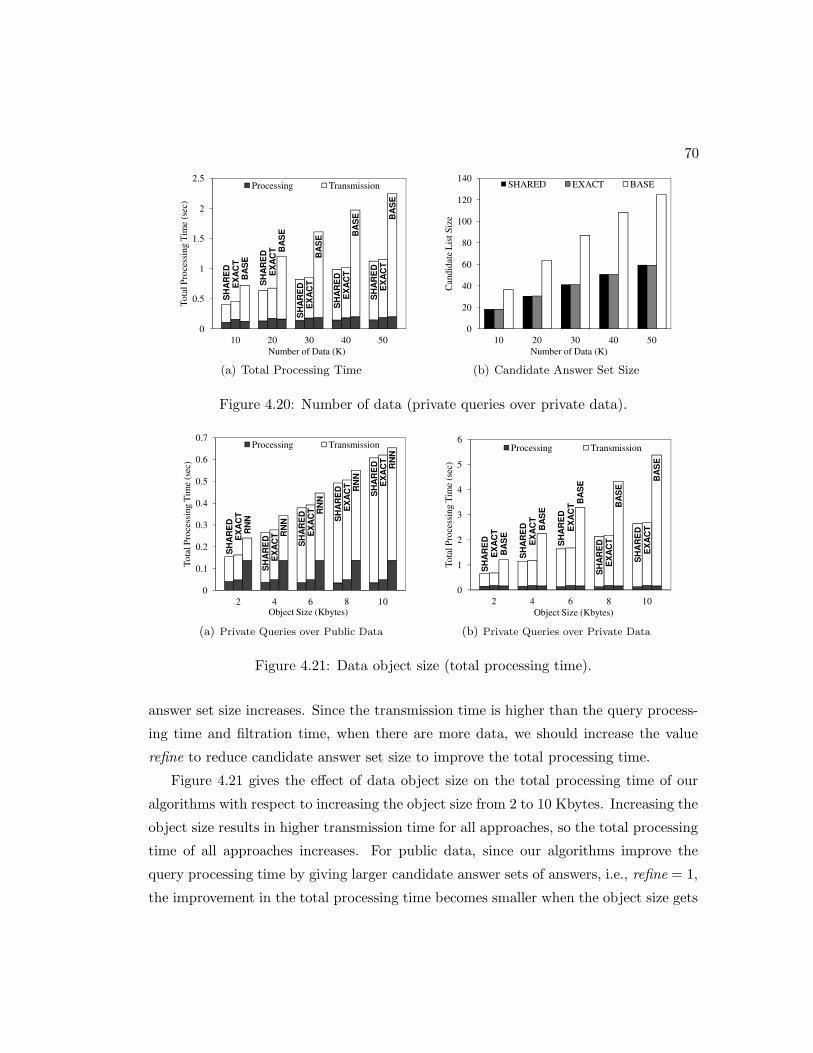
70

SH

AR

ED

SH

AR

ED

SH

AR

ED

SH

AR

ED

SH

AR

ED

EX

AC

T

EX

AC

T

EX

AC

T

EX

AC

T

EX

AC

T

BA

SE

BA

SE

BA

SE B

AS

E BA

SE

0

0.5

1

1.5

2

2.5

10 20 30 40 50

Tota

l Pro

cess

ing

Tim

e (s

ec)

Number of Data (K)



0

20

40

60

80

100

120

140

10 20 30 40 50

Can

dida

te L

ist S

ize

Number of Data (K)

SHARED EXACT BASE


Figure 4.20: Number of data (private queries over private data).

SH

AR

ED

SH

AR

ED SH

AR

ED SH

AR

ED SH

AR

ED

EX

AC

T

EX

AC

T EX

AC

T EX

AC

T EX

AC

T

RN

N

RN

N

RN

N

RN

N

RN

N

0

0.1

0.2

0.3

0.4

0.5

0.6

0.7

2 4 6 8 10

Tota

l Pro

cess

ing

Tim

e (s

ec)

Object Size (Kbytes)


(a) Private Queries over Public Data

SH

AR

ED

SH

AR

ED

SH

AR

ED

SH

AR

ED

SH

AR

ED

EX

AC

T

EX

AC

T

EX

AC

T

EX

AC

T

EX

AC

T

BA

SE

BA

SE

BA

SE

BA

SE

BA

SE

0

1

2

3

4

5

6

2 4 6 8 10

Tota

l Pro

cess

ing

Tim

e (s

ec)

Object Size (Kbytes)


(b) Private Queries over Private Data

Figure 4.21: Data object size (total processing time).

answer set size increases. Since the transmission time is higher than the query process-

ing time and filtration time, when there are more data, we should increase the value

refine to reduce candidate answer set size to improve the total processing time.

Figure 4.21 gives the effect of data object size on the total processing time of our

algorithms with respect to increasing the object size from 2 to 10 Kbytes. Increasing the

object size results in higher transmission time for all approaches, so the total processing

time of all approaches increases. For public data, since our algorithms improve the

query processing time by giving larger candidate answer sets of answers, i.e., refine = 1,

the improvement in the total processing time becomes smaller when the object size gets

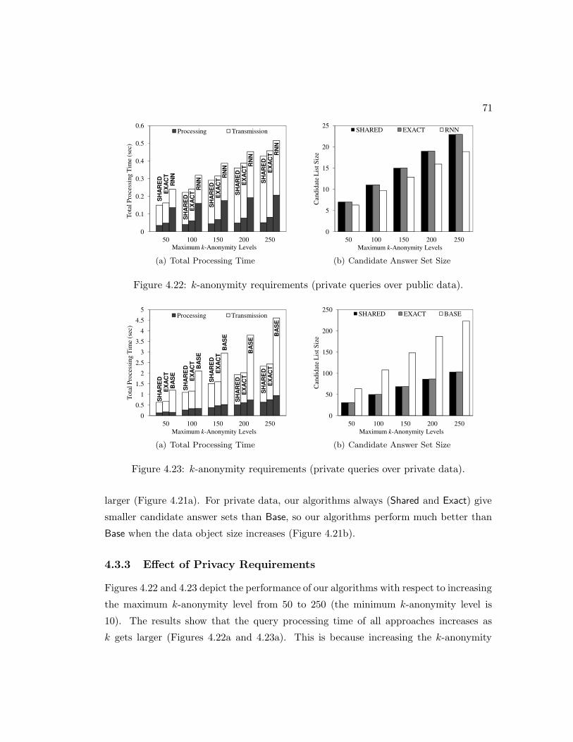
71

SH

AR

ED

SH

AR

ED

SH

AR

ED

SH

AR

ED

SH

AR

ED

EX

AC

T

EX

AC

T EX

AC

T EX

AC

T

EX

AC

T

RN

N

RN

N RN

N RN

N RN

N

0

0.1

0.2

0.3

0.4

0.5

0.6

50 100 150 200 250

Tota

l Pro

cess

ing

Tim

e (s

ec)

Maximum k-Anonymity Levels



0

5

10

15

20

25

50 100 150 200 250

Can

dida

te L

ist S

ize


SHARED EXACT RNN


Figure 4.22: k-anonymity requirements (private queries over public data).

SH

AR

ED

SH

AR

ED

SH

AR

ED

SH

AR

ED

SH

AR

ED

EX

AC

T

EX

AC

T

EX

AC

T

EX

AC

T

EX

AC

T

BA

SE

BA

SE

BA

SE

BA

SE

BA

SE

0

0.5

1

1.5

2

2.5

3

3.5

4

4.5

5

50 100 150 200 250

Tota

l Pro

cess

ing

Tim

e (s

ec)




0

50

100

150

200

250

50 100 150 200 250

Can

dida

te L

ist S

ize


SHARED EXACT BASE


Figure 4.23: k-anonymity requirements (private queries over private data).

larger (Figure 4.21a). For private data, our algorithms always (Shared and Exact) give

smaller candidate answer sets than Base, so our algorithms perform much better than

Base when the data object size increases (Figure 4.21b).

4.3.3 Effect of Privacy Requirements

Figures 4.22 and 4.23 depict the performance of our algorithms with respect to increasing

the maximum k-anonymity level from 50 to 250 (the minimum k-anonymity level is

10). The results show that the query processing time of all approaches increases as

k gets larger (Figures 4.22a and 4.23a). This is because increasing the k-anonymity

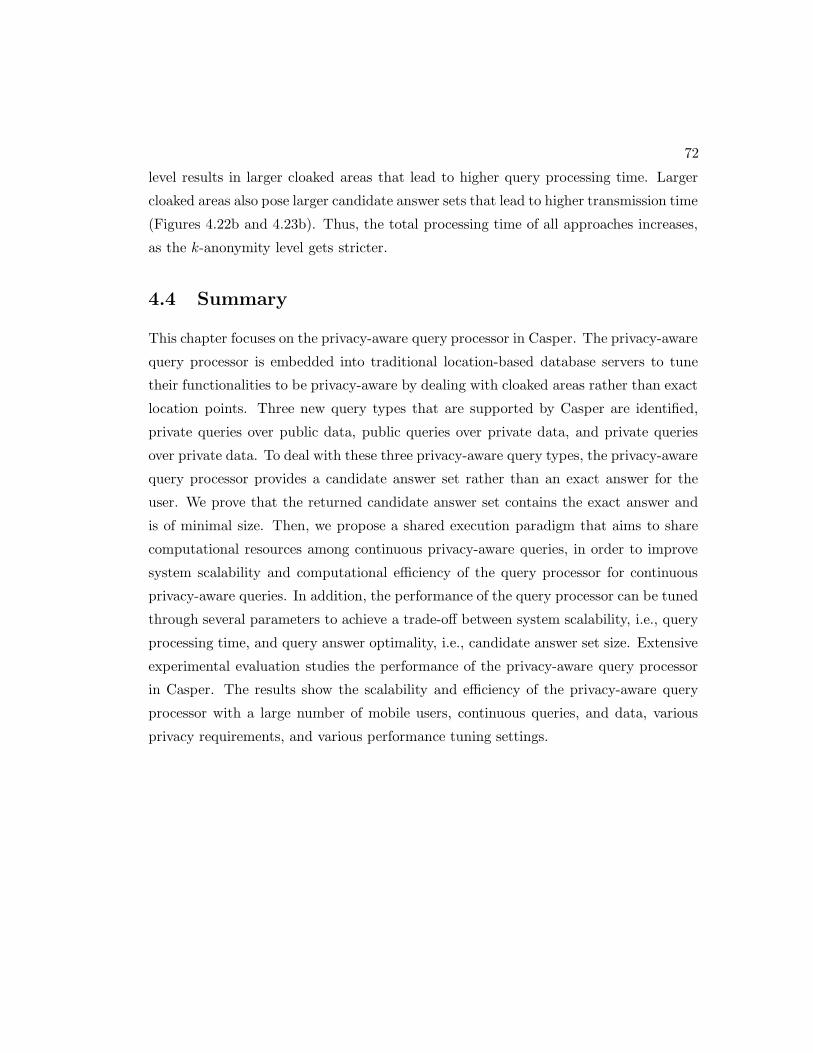
72

level results in larger cloaked areas that lead to higher query processing time. Larger

cloaked areas also pose larger candidate answer sets that lead to higher transmission time

(Figures 4.22b and 4.23b). Thus, the total processing time of all approaches increases,

as the k-anonymity level gets stricter.

4.4 Summary

This chapter focuses on the privacy-aware query processor in Casper. The privacy-aware

query processor is embedded into traditional location-based database servers to tune

their functionalities to be privacy-aware by dealing with cloaked areas rather than exact

location points. Three new query types that are supported by Casper are identified,

private queries over public data, public queries over private data, and private queries

over private data. To deal with these three privacy-aware query types, the privacy-aware

query processor provides a candidate answer set rather than an exact answer for the

user. We prove that the returned candidate answer set contains the exact answer and

is of minimal size. Then, we propose a shared execution paradigm that aims to share

computational resources among continuous privacy-aware queries, in order to improve

system scalability and computational efficiency of the query processor for continuous

privacy-aware queries. In addition, the performance of the query processor can be tuned

through several parameters to achieve a trade-off between system scalability, i.e., query

processing time, and query answer optimality, i.e., candidate answer set size. Extensive

experimental evaluation studies the performance of the privacy-aware query processor

in Casper. The results show the scalability and efficiency of the privacy-aware query

processor with a large number of mobile users, continuous queries, and data, various

privacy requirements, and various performance tuning settings.

Chapter 5

Approximate Range Nearest

Neighbor Queries

In this chapter, we present a new query type, termed approximate range nearest-

neighbor (NN) queries. Although the approximate range NN query is similar to the

private queries over private data, as described in Chapter 4, the approximate range NN

query does not assume a third party placed between the user and the database server

and it can also be applied to the case of users with uncertain location information. NN

queries have been widely used in location-based services (e.g., see [90, 61, 3, 65, 91]).

The problem of traditional NN queries can be defined as follows: “given a set of objects

and a query location point p, find the nearest object(s) to p”; and thus, they are referred

to as point NN queries. Point NN queries have been extended to find all NNs for line

segments [82] and spatial regions [80, 44, 12] that are referred to as linear and range

NN queries, respectively. A linear NN query returns an answer set that includes the

nearest object(s) to every point in a given line segment. On the other hand, a range

NN query returns an answer set that includes the nearest object(s) to every point in a

given spatial region, where the spatial region can be either a rectangular region [80, 12]

or a circular region [44].

Recent research efforts have shown the importance of range NN queries in location-

based services, as it can be applied to the following realistic scenarios:

• Uncertain locations. We have two kinds of location uncertainty, measurement

73

74

imprecision and sampling imprecision. The measurement imprecision is due to

the limitation of the underlying positioning techniques of network environments,

e.g., 2G/3G and Wi-Fi. On the other hand, the sampling imprecision is due

to continuous motion, network delays, and location update frequency even with

highly accurate positioning devices, e.g., GPS. Thus, we have to use a spatial

region where the user is guaranteed to be therein to represent the user location

information in order to capture location uncertainty (e.g., see [92, 93, 94, 95, 96]).

• Privacy-preserving queries. Mobile users are not willing to reveal their exact

location information to location-based service providers, as they want to preserve

their location privacy. The most commonly used privacy-enhancing technique is

to blur the user’s exact location into a spatial region, i.e., spatial cloaking, that

satisfies the user’s specified privacy requirements (e.g., see [44, 12, 32, 34, 39, 36,

97]).

In these two scenarios, the mobile user sends her NN query along with a spatial region as

the query location, i.e., a range NN query. Then, a database server returns an answer

set that includes the nearest object(s) to every point within the spatial region. The

answer set size would substantially increase as the query region gets larger. Unfortu-

nately, the communication bandwidth between the user and the database server is very

limited in a mobile environment, i.e., the downlink bandwidth ranges from 128 kbps at

vehicular speeds to 2 Mbps at stationary or very slow speeds for 3G mobile subscribers.

Transmitting large answer sets to the user would pose very high query response time.

Furthermore, as mobile users receive their answer handheld devices with a small screen,

it is convenient to return to the users very few answers with high quality.

In this chapter, we propose a new approximate range NN query processing algorithm

that enables the user to tune a trade off between query response time and the quality

of query answers. Our proposed algorithm allows the user to specify an approximation

tolerance level t, where we return an answer set A such that each object in A is one

of the t nearest objects of every point in the query region. The larger the value of t,

the smaller the answer set returned by a database server. Thus, the approximation

tolerance level is a tuning parameter that trades off between query response time and

the quality of answers. In the case that t = 1, we return the exact range NN answer of

75

�

�

�

��

(a) 1-NN of each region

��

��

��

��

��

��

��

(b) 2-NN of each region

��

��

��

��

��

(c) 3-NN of each region

Figure 5.1: A motivating example for approximate range NN queries.

maximal size to the user. On the other hand, if t > 1, we return an approximate answer

set, which is smaller than the exact answer, to the user; and thus, the transmission

time of sending the answer set to the user is reduced. Since query response time is

dominated by the communication overhead between the user and the database server,

a larger value of t incurs lower query response time.

Figure 5.1 depicts a motivating example for our problem where we decompose the

query region Q.R of a range NN query Q into disjoint regions and label each region

with its t-NN(s). Figure 5.1a shows the NN of each region. If a user wants to find the

nearest object(s) to Q.R, i.e., the exact range NN query answer, the required answer

set contains the nearest object(s) to every point in Q.R, i.e., A1 = {A,B,C,D,E}.Figure 5.1b shows the 2-NN of each region. If the user is satisfied with the 2-nd nearest

object(s) to Q.R, the answer set A2 should contain at least one object among the 2

nearest objects to every point in Q.R. For example, if A2 = {A,B,C,D}, regardless of

the actual user location within Q.R, the user is guaranteed to receive an object among

her 2 nearest objects. However, we can still do better. For example, if A′2 = {A,C,D},

the user is still guaranteed to receive an object among her 2 nearest objects, regardless

of her actual location within Q.R. Thus, the answer set of minimal size is a minimal

set of objects such that there is at least one object among the 2 nearest objects of each

region. Furthermore, if the user is satisfied with the 3-rd nearest object(s) to Q.R,

i.e., the required answer set A3 should contain at least one object among the 3 nearest

objects of each region, as depicted in Figure 5.1c, where the minimal answer set is

A3 = {A,C}. Therefore, if a user accepts a higher approximation tolerance in a range

NN query answer, the user will receive a smaller answer set and more user convenience.

The main idea of our proposed range NN query processing algorithm is to have an

76

off-line process to pre-compute a set of t-order Voronoi diagrams, from order one to a

predefined maximum order tmax, for a set of stationary data objects, e.g., restaurants,

gas stations and hotels. For a t-order Voronoi diagram, each Voronoi cell is associated

with a distinct set of t objects that are the t nearest objects to every point in the

cell. To efficiently search in a Voronoi diagram, we propose an incomplete pyramid

structure as an access method to index the Voronoi cells. Given a range NN query Q

and an approximation tolerance level t, our proposed on-line range NN query processing

algorithm first determines a set of Voronoi cells V that intersects the query region by

accessing the incomplete pyramid structure of the relevant t-order Voronoi diagram.

Then, the remaining query processing is reduced to a well-known set-covering problem

where we use a greedy approach to select the minimal set of objects, i.e., the answer

set A, from the objects associated with the Voronoi cells in V such that at least one

object from each Voronoi cell in V is selected. As a result, each object in A is one of

the t nearest objects to every Voronoi cell in V, i.e., each object in A is one of the t

nearest objects to every point in the query region. With a larger value of t, there are

more common objects associated among the Voronoi cells in V; and hence, we would

get smaller answer sets that incur lower query response time.

5.1 System Model

In this section, we first formally define our problem, and then present the basic concept

of Voronoi diagrams and the underlying system architecture.

Problem definition. Our problem is defined as follows: given a set of objects, a

range nearest-neighbor query Q with a query region Q.R, and an approximation tolerance

level t, find the minimal set of objects A such that each object in A is one of the t nearest

objects to every point in Q.R.

Voronoi diagrams. Given a set of points S on the plane, which are the Voronoi

sites, the Voronoi diagram of S, denoted as V (S), is a decomposition of the space into

disjoint regions, cells, such that each site si is associated with a cell Vj, denoted as

Vj = {si}, containing all the points in the plane that are closer to si than any other

site in S. In other words, si is the nearest site to every point in Vj . Figure 5.2a depicts

a Voronoi diagram of a set of five sites S = {s1, s2, s3, s4, s5}, V (S). V (S) decomposes

77

��

��

��

��

��

��

��

��

��

��

(a) 1-order Voronoi diagram

��

��

��

��

��

��

��

��

�

��

��

��

(b) 2-order Voronoi diagram

Figure 5.2: The 1-order and 2-order Voronoi diagrams for five sites s1 to s5.

the space into five cells V1, V2, V3, V4, and V5 that are associated with the sites s1, s2,

s3, s4, and s5, respectively. For example, given a point p in cell V1, s1 is the nearest

site to p.

Higher-order Voronoi diagrams. The t-order Voronoi diagram extends the con-

cept of the Voronoi diagram by defining cells based on the t nearest neighbors. The

t-order Voronoi diagram of S, where 1 < t ≤ |S|−1, denoted as Vt(S), is a decomposition

of the space into disjoint cells, such that a distinct set of t sites Si = {si1 , si2 , . . . , sit}is associated with a cell Vj, Vj = {Si}, containing all the points in the plane that have

the sites in Si as their t nearest sites. In other words, Si contains t nearest sites to

every point in Vj. Figure 5.2b depicts the 2-order Voronoi diagram of S, V2(S), that

decomposes the space into seven cells, i.e., V1 = {s1, s3}, V2 = {s1, s2}, V3 = {s2, s3},V4 = {s1, s4}, V5 = {s3, s4}, V6 = {s4, s5}, and V7 = {s3, s5}. For example, given a

point p in cell V3, the sites s2 and s3 are the two nearest sites to p.

System architecture. We consider a mobile environment where mobile users

communicate with a location-based database server through a (2G/3G) cellular network.

The data/control flow of our system is as follows: The mobile user sends range NN

queries to the database server. Our proposed approximate range NN query processing

algorithm that is implemented in the database server computes an answer set, and then

the server sends the answer set to the user. We use the Euclidean distance as our

distance metric.

78

5.2 Approximate Range NN Query Processing

In this section, we first describe an off-line process to compute Voronoi diagrams, from

order one to order tmax, where tmax is the maximum allowable user specified approxi-

mation tolerance level, and present our proposed incomplete pyramid structure that is

used as an access method for each Voronoi diagram. Then, we present an on-line query

processing algorithm for approximate range NN queries.

5.2.1 Building Voronoi Diagrams

We use an off-line process to build t Voronoi diagrams for a set of objects, e.g., restau-

rants, hotels and gas stations, from order one to order tmax, where tmax is the maximum

user specified approximation tolerance level. Thus, the user can specify her desired ap-

proximation tolerance level t from one to tmax. Notice that if t = 1, our algorithm

provides an exact answer set of the minimal size for range NN queries. Given a set

of objects S, building a set of Voronoi diagrams, from order one to order tmax, i.e.,

V1(S), V2(S), . . . , and Vtmax(S), takes O(t2maxN log N) time and O(∑tmax

t=1 t2(N − t))

space, where N is the number of objects in S [98]. After we build the t Voronoi

diagrams, they are stored for later use in our proposed range NN query processing al-

gorithm. For each Voronoi diagram, we maintain a table to store each Voronoi cell with

its associated objects.

5.2.2 Access Method for Voronoi Diagrams

We will construct an incomplete pyramid structure for each Voronoi diagram to support

efficient range search among Voronoi cells. The idea of our proposed incomplete pyramid

structure is that we need to find a set of Voronoi cells V that intersects a given range

query region in order to retrieve their associated objects. Without any index structure,

we have to scan every cell in a Voronoi diagram to find V. When the number of objects

and/or t is large, scanning all cells in a Voronoi diagram would pose a scalability issue.

To this end, we propose an incomplete pyramid structure to overcome this issue. The

construction of an incomplete pyramid structure for each Voronoi diagram includes two

main steps.

79

��

��

��

��

��

��

��

��

��

��

�

��

��

��

�

��

�

��

�

��

��

��

�

��

�

� � � � � � � �

�

�

�

�

�

�

�

�

Figure 5.3: The base level of an incomplete pyramid structure.

Step 1: Base level step. This step decomposes the space into grid cells where

each grid cell C(c, r) is uniquely identified by its column number c and row number r.

Also, we use a hash table, mapping table, that associates each grid cell identity with

a list of Voronoi cells that intersects the grid cell. Figure 5.3 depicts an 8 × 8 grid

structure for the Voronoi diagram given in Figure 5.2a and the corresponding mapping

table. For example, given a grid cell identity C(5, 1), we can retrieve a set of Voronoi

cells that intersects C(5, 1), i.e., V2, V3, and V5.

Step 2: Merge step. This step merges quadtree-like neighbor cells to their parent

if they intersect the same set of Voronoi cells. The idea of this step is to adaptively

determine the height of an incomplete pyramid structure for a Voronoi diagram to min-

imize search time. This is due to the fact that the t Voronoi diagrams we maintain

have different structures, e.g., the number of Voronoi cells and Voronoi cell size distri-

bution, with respect to the number of objects, the object distribution and the degree

of order (t). Thus, the shape of an incomplete pyramid structure would be different for

each computed Voronoi diagram. Other than the base level, each cell C(l, c, r) at upper

levels is identified by the level of the incomplete pyramid structure l, column number c

and row number r. This step uses a bottom-up approach to construct the upper levels

of an incomplete pyramid structure. Starting from the base level, if all quadtree-like

sibling cells (i.e., the cells have the same parent) intersect the same set of Voronoi cells,

they are merged to their parent. The merge process includes three tasks, (i) adding an

entry that associates the parent cell identity with the set of intersected Voronoi cells

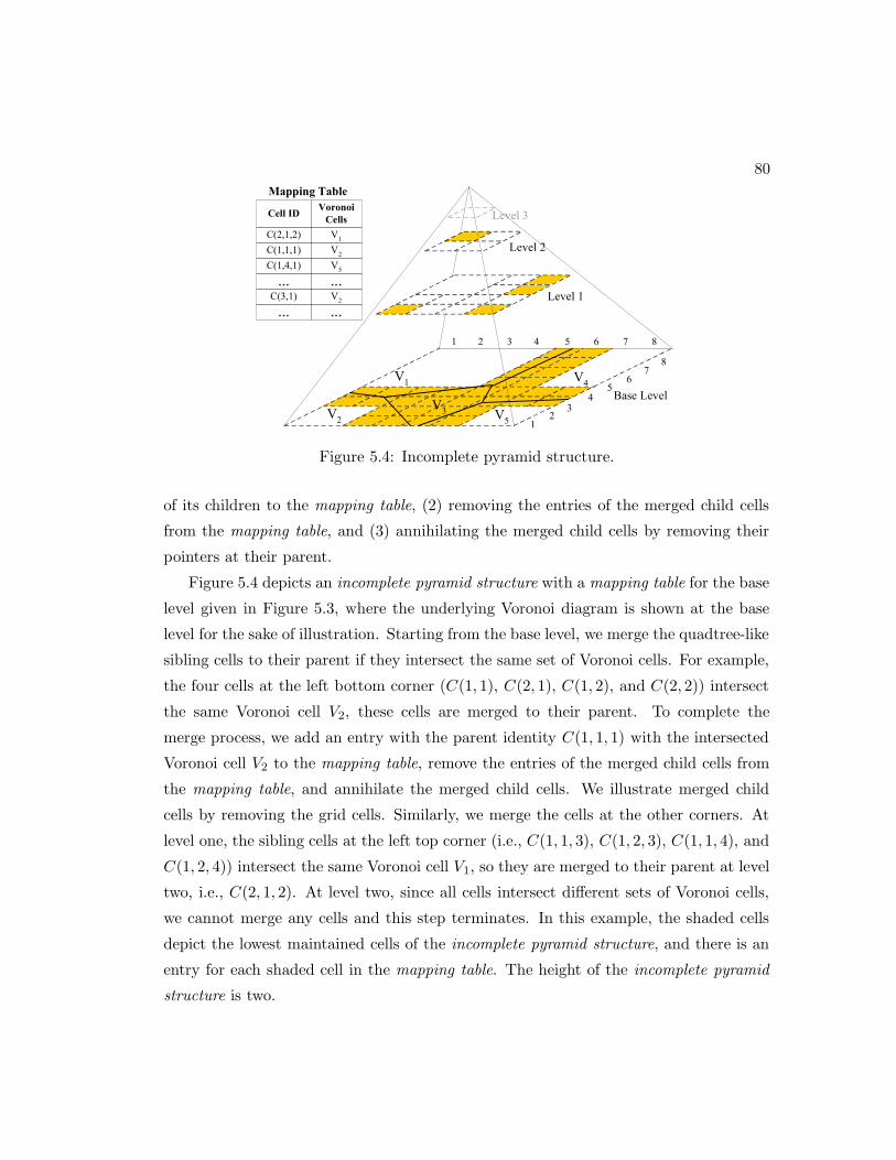
80

��

� ��

��

��

��

��

��

��

� � � � � � � �

��

��

��

��

��

��

��

��

��

��

��

��

��

��

Figure 5.4: Incomplete pyramid structure.

of its children to the mapping table, (2) removing the entries of the merged child cells

from the mapping table, and (3) annihilating the merged child cells by removing their

pointers at their parent.

Figure 5.4 depicts an incomplete pyramid structure with a mapping table for the base

level given in Figure 5.3, where the underlying Voronoi diagram is shown at the base

level for the sake of illustration. Starting from the base level, we merge the quadtree-like

sibling cells to their parent if they intersect the same set of Voronoi cells. For example,

the four cells at the left bottom corner (C(1, 1), C(2, 1), C(1, 2), and C(2, 2)) intersect

the same Voronoi cell V2, these cells are merged to their parent. To complete the

merge process, we add an entry with the parent identity C(1, 1, 1) with the intersected

Voronoi cell V2 to the mapping table, remove the entries of the merged child cells from

the mapping table, and annihilate the merged child cells. We illustrate merged child

cells by removing the grid cells. Similarly, we merge the cells at the other corners. At

level one, the sibling cells at the left top corner (i.e., C(1, 1, 3), C(1, 2, 3), C(1, 1, 4), and

C(1, 2, 4)) intersect the same Voronoi cell V1, so they are merged to their parent at level

two, i.e., C(2, 1, 2). At level two, since all cells intersect different sets of Voronoi cells,

we cannot merge any cells and this step terminates. In this example, the shaded cells

depict the lowest maintained cells of the incomplete pyramid structure, and there is an

entry for each shaded cell in the mapping table. The height of the incomplete pyramid

structure is two.

81

��

��

��

��

��

��

��

��

��

��

� � � � � � � �

�

�

�

�

�

�

�

�

�

(a) Voronoi diagram

��

��

��

��

��

��

��

��

�

��

��

��

� � � � � � � �

�

�

�

�

�

�

�

�

(b) 2-order Voronoi diagram

Figure 5.5: Range NN query processing using Voronoi diagrams.

5.2.3 Online Query Processing Algorithm

The distinct feature of our proposed approximate range NN query processing algorithm

is to enable the user to specify an approximation tolerance t for a range NN query, so

that we provide a minimal answer set A where each object is guaranteed to be one

of the t nearest objects to every point in the query region. If t = 1, we return an

exact answer set with the maximal size to the user. In the case that t > 1, we return

an approximate answer set with a smaller size than the exact one to the user; and

thus, the transmission time of the answer set is reduced. The input of our proposed

algorithm is a range NN query Q, a user specified approximation tolerance level t, and

a t-order Voronoi diagram that is pre-computed by an off-line process (as described in

Section 5.2.1). Figure 7.5 depicts a running example for our proposed algorithm where

the query region of the input range NN query Q is represented as a bold rectangle and

the maximum approximation tolerance level tmax is two. The algorithm consists of two

key steps, range search step (Section 5.2.3) and query-covering step (Section 5.2.3).

Range Search Step

In this step, we retrieve a set of Voronoi cells Vt = {V1, V2, . . . , Vn} that intersects

the query region Q.R and each Voronoi cell in Vt associates with t objects, i.e., Vi =

{si1 , . . . , sit} (1 ≤ i ≤ n). We use a top-down approach to traverse an incomplete

82

��

��

��

��

��

��

��

��

�

��

��

��

��

��

��

� ��

��

��

��

Figure 5.6: Example of a range search in the incomplete pyramid structure (Figure 5.4).

pyramid structure. Initially, at the highest maintained level of the incomplete pyramid

structure of the t-order Voronoi diagram, we find a set of grid cells that intersects

Q.R, and then recursively search each of these grid cells. During a recursive search,

if an encountered grid cell C that intersects Q.R is at the lowest maintained level or

base level of the incomplete pyramid structure, we retrieve the set of Voronoi cells that

intersects C from the mapping table, and then return it. Otherwise, we recursively

search the four child cells of C.

Figure 5.6 illustrates the range search step for the running example depicted in

Figure 7.5a where t = 1. For the sake of illustration, we only show the grid cells

intersecting the query region Q.R, and the grid cells at the lowest maintained level or

base level of the incomplete pyramid structure (as depicted in Figure 5.4) are represented

shaded nodes. As shown in Figure 5.4, the highest maintained level of the incomplete

pyramid structure is level two where we start the range search step. Since all grid cells

at level two, i.e., C(2, 1, 1), C(2, 1, 2), C(2, 2, 1) and C(2, 2, 2), intersect Q.R, we will

recursively search these grid cells. For C(2, 1, 1), only one child cell C(1, 2, 2) intersects

Q.R, so we search their child cells C(3, 3), C(3, 4), C(4, 3), and C(4, 4) at the base level.

Since all these child cells intersect Q.R, we retrieve the Voronoi cells that intersect them

from the mapping table and return the set of retrieved Voronoi cells. As C(2, 1, 2) is

at the lowest maintained level, we retrieve the Voronoi cells that intersects C(2, 1, 2)

from the mapping table without further search. Then, we search the grid cell C(2, 2, 1)

where it has two child cells C(1, 3, 2) and C(1, 4, 2) intersecting Q.R. Since all child

cells of C(1, 3, 2) and C(1, 4, 2) at the base level intersect Q.R, we retrieve the Voronoi

cells that intersect them from the mapping table and return the retrieved Voronoi cells.

Similarly, we search the grid cell C(2, 2, 2). As a result, the set of Voronoi cells that

83

Algorithm 4 Query-Covering Step

1: function QueryCovering (RNNQuery Q, ToleranceLevel t, VoronoiCellSet Vt)2: AnswerSet A ← {∅}3: Construct an inverted list of Vt, i.e., L(Vt) = {L(s1), L(s2), . . . , L(sm)}, where

L(si) = {Vi1 , Vi2 , . . . , Vi|L(si)|} and 1 ≤ i ≤ m

4: while L(Vt) 6= {∅} do5: Select the object si ∈ L(Vt) with the largest |L(si)|6: for each object sj ∈ L(Vt) (i 6= j) do7: L(sj)← L(sj)− L(si)8: if L(sj) = {∅} then9: L(Vt)← L(Vt)− {L(sj)}

10: end if11: end for12: A ← A ∪ {si}13: L(Vt)← L(Vt)− {L(si)}14: end while15: return A

intersects Q.R is V1 = {V1, V2, V3, V4, V5}. For the other running example where t = 2,

the range search step searches the incomplete pyramid structure of the 2-order Voronoi

diagram and the set of Voronoi cells that intersects Q.R is V2 = {V1, V3, V4, V5, V6, V7}.

Query-Covering Step

Algorithm 4 gives the pseudo code of this step where we aim to compute the minimal

set of objects in which each object is one of the t nearest objects to every point in the

query region Q.R. First, we construct an inverted list of the set of Voronoi cells Vt

retrieved from the previous step, L(Vt) (Line 3). In the inverted list L(Vt), each object

si has a list of Voronoi cells L(si) = {Vi1 , . . . , Vim} (m ≤ n), where si is associated with

Vij (1 ≤ j ≤ m).

Figure 5.7a depicts the inverted list of our running example for t = 1, as given in

Figure 7.5a, where the Voronoi cells in V1 with their associated objects retrieved from

the range search step are V1 = {s1}, V2 = {s2}, V3 = {s3}, V4 = {s4}, and V5 = {s5}.The inverted list of V1 is L(V1) = {L(s1) = {V1}, L(s2) = {V2}, L(s3) = {V3}, L(s4) =

{V4}, L(s5) = {V5}}. On the other hand, Figure 5.7b depicts the inverted list of our

running example for t = 2, as shown in Figure 7.5b where the Voronoi cells in V2

84

��

��

��

��

��

�

��

�

��

��

��

��

��

��

��

�

��

�

��

��

��

� ��

��

(a) Voronoi cell set V1

��

��

��

��

��

��

��

��

� ��

��

��

��

��

�

��

��

��

��

��

��

��

��

��

��

(b) Voronoi cell set V2

Figure 5.7: Inverted lists.

with their associated objects retrieved from the range search step are V1 = {s1, s3},V3 = {s2, s3}, V4 = {s1, s4}, V5 = {s3, s4}, V6 = {s4, s5}, and V7 = {s3, s5}. The

inverted list of V2 is L(V2) = {L(s1) = {V1, V4}, L(s2) = {V3}, L(s3) = {V1, V3, V5, V7},L(s4) = {V4, V5, V6}, L(s5) = {V6, V7}}.

After constructing the inverted list of Vt, L(Vt), our objective is to select the minimal

set of objects from L(Vt) such that every Voronoi cell in Vt has at least one associated

object selected in the answer set. In other words, we consider the items in the inverted

list as sets and the Voronoi cells in Vt as elements, and then select a minimum number

of sets so that the selected sets contain all the elements that are contained in any of

the sets in the inverted list. Thus, our problem can be reduced to a well-known set-

covering problem. Since computing the optimal solution for the set-covering problem

is NP-hard [99], we use a greedy approach to compute an answer set. Basically, the

greedy approach selects an object with the largest set of Voronoi cells, and then remove

the Voronoi cells associated with the selected object from other objects’ lists. Then, the

selected object and the objects with an empty list are removed from the inverted list.

We repeat this procedure until the inverted list is empty (Lines 4 to 14 in Algorithm 4).

The set of selected objects is returned as the answer set to the user.

In our running example for t = 1, i.e., the user wants to have an exact query answer,

the query-covering step simply add all objects in the inverted list L(V1) (Figure 5.7a)

to the answer set, i.e., A1 = {s1, s2, s3, s4, s5}. On the other hand, Figure 5.8 depicts

the query-covering step for our running example for t = 2, based on the inverted list of

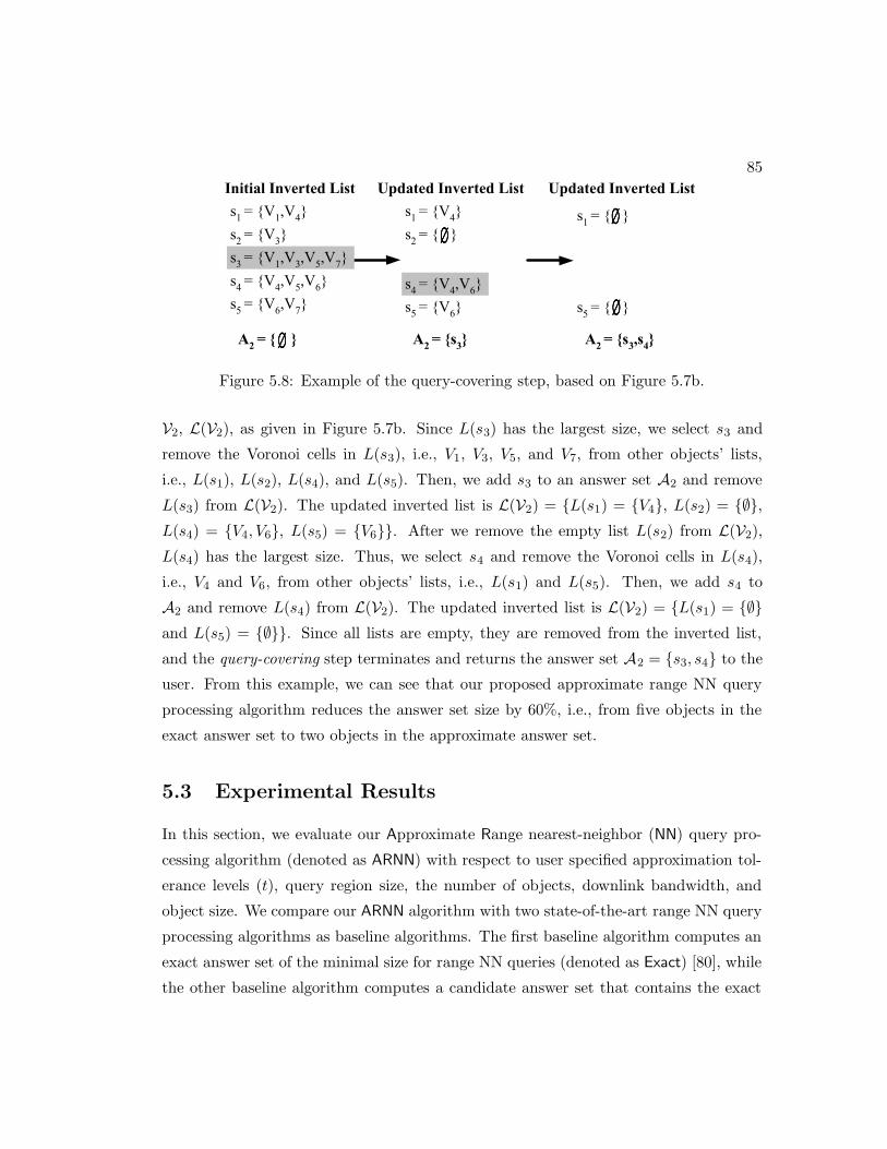
85

� ∅∅∅∅

��

��

��

�

��

��

��

��

��

��

��

��

� ∅∅∅∅ ��

�

��

��

��

��

�

��

��

��

� ∅∅∅∅ ��

� ∅∅∅∅

��

��

��

��

Figure 5.8: Example of the query-covering step, based on Figure 5.7b.

V2, L(V2), as given in Figure 5.7b. Since L(s3) has the largest size, we select s3 and

remove the Voronoi cells in L(s3), i.e., V1, V3, V5, and V7, from other objects’ lists,

i.e., L(s1), L(s2), L(s4), and L(s5). Then, we add s3 to an answer set A2 and remove

L(s3) from L(V2). The updated inverted list is L(V2) = {L(s1) = {V4}, L(s2) = {∅},L(s4) = {V4, V6}, L(s5) = {V6}}. After we remove the empty list L(s2) from L(V2),

L(s4) has the largest size. Thus, we select s4 and remove the Voronoi cells in L(s4),

i.e., V4 and V6, from other objects’ lists, i.e., L(s1) and L(s5). Then, we add s4 to

A2 and remove L(s4) from L(V2). The updated inverted list is L(V2) = {L(s1) = {∅}and L(s5) = {∅}}. Since all lists are empty, they are removed from the inverted list,

and the query-covering step terminates and returns the answer set A2 = {s3, s4} to the

user. From this example, we can see that our proposed approximate range NN query

processing algorithm reduces the answer set size by 60%, i.e., from five objects in the

exact answer set to two objects in the approximate answer set.

5.3 Experimental Results

In this section, we evaluate our Approximate Range nearest-neighbor (NN) query pro-

cessing algorithm (denoted as ARNN) with respect to user specified approximation tol-

erance levels (t), query region size, the number of objects, downlink bandwidth, and

object size. We compare our ARNN algorithm with two state-of-the-art range NN query

processing algorithms as baseline algorithms. The first baseline algorithm computes an

exact answer set of the minimal size for range NN queries (denoted as Exact) [80], while

the other baseline algorithm computes a candidate answer set that contains the exact

86

Table 5.1: Parameter settings.

Parameter Default Value Range

Approximation tolerance (t) 4 1 to 10Number of objects 200 100 to 300Query region size (0.05l)2 (0.008l)2 to (0.256l)2 (where l = 1000)

Downlink bandwidth 384 kbps 128 kbps to 2 MbpsObject size 10 Kbytes 0.5 Kbytes to 20 Kbytes

answer for range NN queries (denoted as Casper) [12].

We have two performance measures: (1) total processing time that includes the query

processing time at the database server and the transmission time of sending the answer

set to the user, and (2) answer set size that is the average number of objects returned

in the answer sets. The answer set size is important as it indicates communication

overhead and the power consumed by the user device to receive the answer set and user

convenience.

In all experiments, we assume that the user communicates with a database server

through a 3G cellular network. The downlink (i.e., from the database server to the user)

bandwidth varies with respect to the user mobility speed, i.e., 128 kbps (i.e., kbits per

second) at vehicular speeds, 384 kbps at pedestrian speeds, 2 Mbps at stationary or

very slow movement speeds. Unless mentioned otherwise, the experiments consider 200

objects in a square space of a length l = 1000. The mobile user moving at pedestrian

speeds (i.e., the downlink bandwidth is 384 kbps) issues 1,000 range NN queries, and

the object size is 10 Kbytes. The default user specified approximation tolerance level

(t) is four and the query region size is 0.05l×0.05l. Table 9.1 summarizes the parameter

settings.

5.3.1 Effect of Approximation Tolerance Levels

Figure 9.10 depicts the performance of our proposed algorithm (ARNN) with respect to

varying the approximation tolerance level (t) from 1 to 10. The performance of the base-

line algorithms (Casper and Exact) is not affected by varying the value of t. Figure 9.10a

gives the number of objects returned in the answer set, while Figure 9.10b indicates the

total processing time that includes the query processing time at the database server and

87

�

�

�

�

�

�

� � � � � ��

��

��

��

��

(a) Answer set size

�

��

��

��

��

�

� � � � � ��

��

� ��

��

�� !��

(b) Total Processing time

�

��

�

��

�

��

�

��

��

��

�� !��

"#$ $ %��!�� &'��

(c) Tolerance level: t = 2

�

��

�

��

�

��

�

��

��

��

�� !��

"#$ $ %��!�� &'��

(d) Tolerance level: t = 10

Figure 5.9: Approximation tolerance levels (t).

the transmission time of sending the answer set to the user. Figure 9.10a shows that

ARNN effectively reduces the answer set size as t gets larger. When t = 2 (t = 10),

ARNN reduces the size of the answer sets given by Casper and Exact by 34.3% and 66%

(79.3% and 89.3%), respectively. Since the transmission time is much higher than the

total processing time, the total processing time of ARNN decreases as t gets larger (Fig-

ure 9.10b). Figures 9.10c and 9.10d show that ARNN performs better than the baseline

algorithms for all mobility speeds. Since ARNN effectively reduces the answer set size,

when the downlink bandwidth is more limited, ARNN performs much better than Casper

and Exact.

88

�

�

��

��

��

��

��

��

��

��

��

��

��

��

� ��

��

��

� �!�

(a) Answer set size

�

�

�

�

�

��

��

��

��

��

� ��

!�" "

# �$��

%& ��

(b) Total processing time

�

��

��

��

��

�

��

��

��

��

�� !��

"#$ $

%��!��

&'��

(c) Query region size: (0.008l)2

�

�

��

��

��

��

��

��

��

��

� ��

��

!"# #

$��

%&��

(d) Query region size: (0.256l)2

Figure 5.10: Query region size.

5.3.2 Effect of Query Region Size

Figure 5.10 depicts the performance of our proposed algorithm (ARNN) with respect

to increasing the query region size from (0.008l)2 to (0.256l)2, where l = 1000. Fig-

ure 5.10a shows that the answer set of all algorithms gets larger as the query region size

increases. With small query regions, i.e., (0.008l)2, the answer set size of ARNN is 94.7%

and 59.8% smaller than Casper and Exact, respectively. For large query regions, i.e.,

(0.256l)2, the answer set size of ARNN is 442.1% and 145.3% smaller than Casper and

Exact, respectively. Thus, ARNN performs much better than the baseline algorithms

for larger query regions. Since the transmission time is much higher than the total

processing time, ARNN outperforms the baseline algorithms in terms of query response

89

�

�

�

�

�

�

�

��

��

� ��

��

�� !��

(a) Answer set size

�

��

��

��

��

�

��

��

��

��

��

!"� � # �$�� %& ��

(b) Total processing time

�

��

�

��

�

��

��

��

��

�� !��

"#$ $ %��!�� &'��

(c) 100 objects

�

��

�

��

�

��

�

��

��

��

��

�� !��

"#$ $ %��!�� &'��

(d) 300 objects

Figure 5.11: Number of objects.

time (Figure 5.10b). Figures 5.10c and 5.10d depict that ARNN effectively reduces the

total processing time of the baseline algorithms regardless of user mobility speeds.

5.3.3 Effect of Number of Objects

Figure 5.11 gives the performance of our proposed algorithm (ARNN) with respect to

varying the number of objects from 100 to 300. When the number of objects increases,

there are more nearest objects to the query region; and thus, the answer set size of

all algorithms gets larger (Figures 5.11a). Similar to the previous experiments, the

transmission time is much higher than the total processing time. Since the answer set

size of ARNN is smaller than the baseline algorithms Casper and Exact, ARNN incurs the

90

�

��

��

��

��

��

��

��

��

��

�� !��

"#$ $

%��!��

&'��

(a) 0.5 KB

�

�

�

�

�

�

�

��

��

��

�� !��

"#$ $

%��!��

&'��

(b) 20 KB

Figure 5.12: Object size.

lowest total processing time for any number of objects (Figures 5.11b). Likewise, ARNN

effectively reduces the answer set size, the total processing time of ARNN is better than

Casper and Exact for all user mobility speeds, as depicted in Figures 5.11c and 5.11d.

5.3.4 Effect of Object Size

Figure 5.12 depicts the performance of our proposed algorithm (ARNN) with respect to

the object size of 0.5 and 20 Kbytes. Since varying the object size does not affect the

answer set size, the answer set size of all algorithms is the same as the case that t = 4 in

Figure 9.10a. It is interesting to see that the transmission time is much higher than the

total processing time even if the object size is small and the answer set is sent to the user

through the downlink with the largest possible bandwidth, i.e., 2 Mbps. Therefore, the

results indicate that reducing the answer set size is an effective way to improve query

response time. This is the motivation of our proposed algorithm ARNN that aims to

minimize the answer set size while guaranteeing that the answer set is satisfied with the

user specified approximation tolerance level t.

5.3.5 Effect of Communication Bandwidth

Figures 5.13 and 5.14 give the comprehensive evaluation of our proposed algorithm

(ARNN) with respect to all parameters for users moving at vehicular speeds and very

slow speeds, respectively. Although Casper gives the best query processing time, it

91

�

��

�

��

�

��

�

� � � � ��

��

��

��

�� !�� "# ��

(a) Approximation tolerance

�

�

��

��

��

��

��

��

��

��

��

� ��

!�" "

# �$��

%& ��

(b) Query region size

�

��

�

��

�

��

�

��

��

��

��

��

�� !�� "#�

(c) Number of objects

�

�

�

�

�

�

�

� � � � � ��

��

��

� ��

!"# #

$��%��

&'��

(d) Object size

Figure 5.13: Downlink bandwidth at vehicular speeds (128 kbps).

suffers from very high transmission time. This is because the candidate answer set

provided by Casper is much larger than the answer set of ARNN and Exact. Thus, the

total processing time of Casper is always worse than ARNN and Exact. Since ARNN

provides approximate answers that satisfy the user specified approximation tolerance

level, the answer set size of ARNN is smaller than the exact answer set provided by

Exact. As a result, ARNN performs better than Casper and Exact in terms of the total

processing time for all parameter settings.

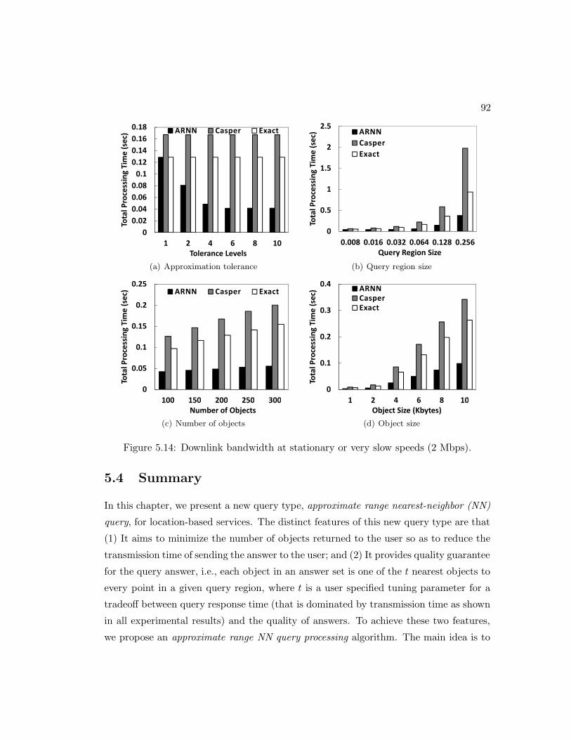
92

�

��

��

��

��

��

��

��

��

��

� � � � � ��

��

� ��

��

�� !��

(a) Approximation tolerance

�

��

�

��

�

��

��

��

��

� ��

!�" "

# �$��

%& ��

(b) Query region size

�

��

��

��

��

��

��

��

��

��

�� !�� "#�

(c) Number of objects

�

��

��

��

��

� � � � � ��

��

��

� ��

!"# #

$��%��

&'��

(d) Object size

Figure 5.14: Downlink bandwidth at stationary or very slow speeds (2 Mbps).

5.4 Summary

In this chapter, we present a new query type, approximate range nearest-neighbor (NN)

query, for location-based services. The distinct features of this new query type are that

(1) It aims to minimize the number of objects returned to the user so as to reduce the

transmission time of sending the answer to the user; and (2) It provides quality guarantee

for the query answer, i.e., each object in an answer set is one of the t nearest objects to

every point in a given query region, where t is a user specified tuning parameter for a

tradeoff between query response time (that is dominated by transmission time as shown

in all experimental results) and the quality of answers. To achieve these two features,

we propose an approximate range NN query processing algorithm. The main idea is to

93

have an off-line process to compute Voronoi diagrams, from order one to order tmax,

where tmax is the maximum allowable user specified approximation tolerance level, and

then build our proposed incomplete pyramid structure as an access method for each

Voronoi diagram. Given a range NN query and an approximation tolerance level t, our

on-line query processing algorithm accesses the incomplete pyramid structure of the t-

order Voronoi diagram to retrieve a set of Voronoi cells that intersects the query region

and the t nearest objects to each Voronoi cell. Then, the remaining query processing is

reduced to a set-covering problem where we use a greedy approach to find a minimal

answer set. Extensive experimental results show that our proposed algorithm is scalable

in terms of query processing time, and effective to reduce query response time compared

with the state-of-the-art techniques while guaranteeing that the answer set satisfies the

user desired approximation tolerance level.

Chapter 6

Query-Aware Location

Anonymization in Road Networks

In this chapter, we extend the functionalities of the Casper system, i.e., the location

anonymizer and the privacy-aware query processor, in road network environments. Sev-

eral techniques are proposed to anonymize the user location information through false

locations (e.g., [43, 45, 81]), space transformation (e.g., [78, 79]), or spatial cloaking

(e.g., [32, 34, 33, 19, 35, 36, 38, 39, 37, 23, 44, 12, 47, 48]). This chapter focuses on the

spatial cloaking technique as it is the most commonly used technique and is applicable

to various problem settings (e.g., distributed/peer-to-peer environments [19, 38, 39],

sensor networks [23], trajectories [48], and continuous queries [33, 47]).

Unfortunately, almost all previously proposed location anonymization techniques

suffer from two main drawbacks: (1) The location anonymization process is designed

completely independent from the underlying query processor. As a result, some of these

techniques may end up anonymizing the user location to an extent where it is either

very inefficient to execute a location-based query as a large number of queries need

to be sent to the server [45, 81] or specialized query processing techniques need to be

developed [78, 44, 79, 12]. (2) All techniques are designed only for the Euclidean space.

Applying these techniques to the road network environment results in privacy leakage.

Figure 6.1a depicts such a case where user q needs to be four anonymous with a cloaked

area of at least four grid cells. The gray area represents the cloaked area that could

94

95

�

(a) Euclidean Space

�

(b) Road Network

Figure 6.1: Spatial cloaking for the Euclidean space.

be provided by a location anonymization technique designed for the Euclidean space

(e.g., [32, 36, 37, 44, 12]). With such a cloaked area, an adversary knows that the user

can be anywhere in the gray area. Figure 6.1b shows the same example with the drawing

of the underlying road network. Since all the four users are in the same road segment,

an adversary can pinpoint the exact road segment of user q. Thus, the cloaked area

violates the area privacy requirement, i.e., the user cannot be anywhere in the cloaked

area, as the user has to be in a single road segment only. The only previous work that

addresses location privacy in a road network [100] suffers from the same drawbacks as

it solely relies on using an Euclidean-based anonymization technique while considering

the road network in the query processing only.

In this chapter, we overcome the above two main drawbacks by proposing a new

location anonymization algorithm that (a) is designed specifically for the road network

environment, and (b) not only aims to satisfy the user privacy requirements, but it is also

“query-aware” as it aims to balance between the query execution cost and the quality of

services that we can get from the server. The main idea of our proposed “query-aware”

location anonymization technique is to blur a user location into a cloaked set of con-

nected road segments S such that S satisfies the user specified privacy requirements,

k-anonymity and minimum length Lmin. The k-anonymity requirement indicates in-

clude at least k users while the minimum length l length Lmin requirement indicates

96

that the total length of in S must be at least l. As the database server only database

server only knows about a cloaked segment set S as a user’s location information, it

has to compute an answer set A includes the exact query answer should the user be

anywhere within S. The smaller the size of the returned answer set A, the better qual-

ity the server will provide. Thus, the quality of services is measured by the size of the

returned answer set. To achieve our goals, we design a new objective cost function that

encapsulates the query execution cost for both K-nearest-neighbor and range queries

with the answer quality. Then, the objective of our road network location anonymiza-

tion algorithm boils down to finding a cloaked set of road segments S that minimizes

our developed objective cost function while satisfying the user privacy requirements.

We present two versions of our proposed location anonymization algorithm. The

first version is a pure greedy approach where we repeatedly select road segments to be

included in a cloaked segment set S based on minimizing our developed objective cost

function. Although the pure greedy approach is simple and efficient, its deterministic

property may suffer from a reverse engineering attack where an adversary may crack the

system to know the objective cost function. To avoid such an attack, we propose another

version of our algorithm, termed randomized greedy approach, where we inject some

randomness into the greedy approach. To accommodate for cases of high workloads,

e.g., traffic congestions and rush hours, we propose a shared execution paradigm that

boosts the system scalability in terms of supporting large numbers of queries received

within a short time period. The main idea of the shared execution paradigm is to

maximize the number of shared road segments among the users’ cloaked segment sets.

By doing so, location-based queries at the shared road segments will be executed only

once for multiple queries.

6.1 System Model

In this section, we first give the preliminaries of this paper. Then, we describe the

underlying system architecture that consists of three main entities, mobile users, location

anonymizer, and location-based database server.

Preliminaries. The proposed location anonymization algorithm mainly blurs a

user’s location into a cloaked set of road segments S that is defined as a set of

97

connected road segments where the requesting user is residing therein, such that S

satisfies the user specified privacy requirements. In a cloaked set S, a vertex v is a

closed vertex if all edges connected to v are included in S; otherwise, v is an open

vertex. The underlying road network is modeled as a connected graph G = (V,E),

where V is a vertex set that represents the intersection and endpoints of the road

segments, while E is an edge set that represents the road segments.

Mobile users/privacy requirements. Mobile users register with the system

by specifying their personalized privacy requirements, i.e., k-anonymity and minimum

length Lmin. k-anonymity privacy requirement indicates user wants to be k-anonymous,

i.e., indistinguishable among k users. The minimum length privacy requirement Lmin

indicates that the minimum resolution of the blurred location the total length of the

road segments in S is at least . Thus, a user’s location must be blurred into a cloaked set

a cloaked set S that contains at least k users and the total length of the road segments

in S is at least Lmin.

Location anonymizer. The location anonymizer is a trusted third party placed be-

tween mobile users and the location-based database server. We assume that the location

anonymizer is placed at some cellular service provider through which the mobile users

have access to location-based service providers. Furthermore, the location anonymizer

maintains an edge table that is a hash-table on edge ID [67]. For each edge e, the tuple

in the edge table stores (a) its endpoints, (b) its length, (c) the set of edges connected

to each of its endpoints, and (d) the list of objects currently residing in e. Basically, the

location anonymizer blurs the location information of a user’s query into a cloaked set of

road segments S such that S satisfies the user’s privacy requirements. While blurring the

location information, the location anonymizer also removes any user identity to ensure

the pseudonymity of the location information [9]. Then, the location anonymizer sends

the anonymized query with the cloaked segment set to the database server. After the

location anonymizer gets a candidate answer set from the database server, it computes

the exact answer from the candidate answer set and sends the exact answer to the user.

Location-based database server. The location-based database server is placed at

an untrustworthy service provider and has the capacity to deal with private queries along

with cloaked sets of road segments. Since the private queries can be easily boiled down to

traditional K-nearest-neighbor (K-NN) and range queries (described in Section 6.2), the

98

query processor embedded inside the database server only needs to employ any existing

K-NN and range query algorithms designed for road networks (e.g., [101, 102, 103]). Fur-

thermore, the database server also maintains an edge table as in the location anonymizer.

Instead of returning an exact answer, the database server returns a candidate answer

set that is guaranteed to contain the exact answer to the location anonymizer regardless

of the exact user location within the given cloaked segment set S.

6.2 Cost Model for Private Queries

This section develops the cost model for both private K-nearest-neighbor (K-NN) and

range queries. This cost model will be used later by the location anonymizer (Sec-

tion 6.3) to find a cloaked set of road segments S that balances between minimizing the

developed cost function and the query answer quality while satisfying the user privacy

requirements. Throughout this section, we use the following terminologies and assump-

tions: (a) We assume only an existing spatio-temporal query processor embedded inside

the database server to deal with private K-NN and range queries. Thus, the query pro-

cessor can employ any existing K-NN and range query processing algorithms designed

for road networks (e.g., [101, 104, 102, 103]). (b) For any cloaked set of road segments

S, we define two functions Vo(S) and E(S) that return the number of open vertices (i.e.,

vertices where some of its connected edges are not included in S ) and the number of

edges in S, respectively. (c) Without loss of generality, we assume that all K-NN and

range queries ask about the same type of target objects (e.g., gas stations, taxis, or

restaurants). There are T such target objects and R road segments in the system. The

information about the number of target objects is given by the database server as hints.

For all vertices and edges in the road network, d and l represent the average degree of

connectivity of a vertex v (i.e., the number of edges connected to v) and the average

edge length, respectively.

6.2.1 Private K-Nearest-Neighbor Queries

A typical example of a K-nearest-neighbor (K-NN) query is “find the K nearest objects

of my location q = (x, y)”. However, with the anonymization process, the K-NN query

is transformed to a private one, i.e., “find the K nearest objects of my location, given

99

that my location is somewhere in a cloaked set of road segments S”.

Algorithm. An algorithm for a private K-NN query with a cloaked set of road

segments S will find a candidate answer set where the exact answer of the original query

is guaranteed to be in the candidate answer set regardless of the actual user location

within S. To facilitate the development of the query cost model, given a cloaked set of

road segments S, we divide the query processing algorithm of private K-NN queries into

two steps: (1) Range Search Step. In this step, we mainly execute a traditional range

query of the form “find all target objects located within the road segments in S” where

we add all target objects within S to the candidate answer set. (2) External Search

Step. In this step, we mainly execute a traditional K-NN query at each open vertex in

S, i.e., “find the closest K target objects to a vertex v”, where we add the answers of

these queries to the candidate answer set.

Thus, the execution of one private K-NN query boils down to executing one tradi-

tional range query and a set of traditional K-NN queries. Figure 6.2 depicts a private

K-NN query (K = 1), where the actual query location Q is represented as a triangle

located in edge v4v6. The cloaked segment set S of Q includes three edges v3v4, v4v6,

and v4v9, one closed vertex v4, and three open vertices v3, v6, and v9. Figure 6.2a de-

picts the range search step where we add all target objects of the three edges in S, o3

to o7, to the candidate answer set. Figure 6.2b depicts the external search step where

the nearest target object to each open vertex in S (enclosed in rectangles) is added to

the candidate answer set. The nearest target object of the open vertices v3, v6, and v9

are o2, o7, and o8, respectively. As a result, the answer of the private K-NN query is a

candidate answer set that contains seven objects o2 to o8. Notice that the exact answer,

according to the exact location of Q, is o7 which is included in the candidate answer

set.

Cost model. The execution cost of a private K-NN query is the sum of the execution

cost of the range search and external search steps. We will present the cost in terms of the

number of edges whose information is retrieved through the edge table data structure as

described in Section 6.1. For the range search step, we need to retrieve the information

(i.e., target objects) of all edges in S. This step results in a straightforward cost of

E(S), i.e., the number of edges in S. For the external search step, we will first consider

the cost of issuing a traditional K-NN query at one open vertex. Without the knowledge

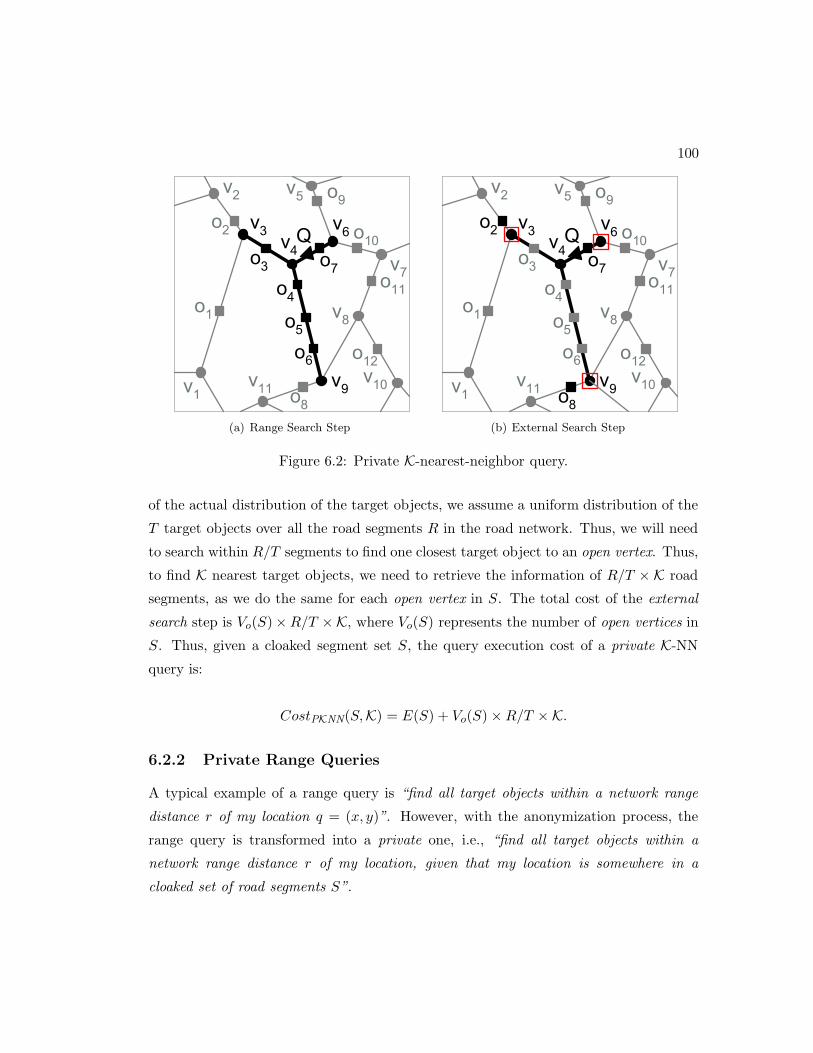
100

��

��

��

��

��

��

��

��

��

�

��

�

�

�

�

�

�

��

��

�

�

�

(a) Range Search Step

��

��

��

��

��

��

��

��

��

�

��

�

�

�

�

�

�

��

��

�

�

�

(b) External Search Step

Figure 6.2: Private K-nearest-neighbor query.

of the actual distribution of the target objects, we assume a uniform distribution of the

T target objects over all the road segments R in the road network. Thus, we will need

to search within R/T segments to find one closest target object to an open vertex. Thus,

to find K nearest target objects, we need to retrieve the information of R/T × K road

segments, as we do the same for each open vertex in S. The total cost of the external

search step is Vo(S)×R/T ×K, where Vo(S) represents the number of open vertices in

S. Thus, given a cloaked segment set S, the query execution cost of a private K-NN

query is:

CostPKNN(S,K) = E(S) + Vo(S)×R/T ×K.

6.2.2 Private Range Queries

A typical example of a range query is “find all target objects within a network range

distance r of my location q = (x, y)”. However, with the anonymization process, the

range query is transformed into a private one, i.e., “find all target objects within a

network range distance r of my location, given that my location is somewhere in a

cloaked set of road segments S”.

101

Algorithm. Similar to the case of private K-NN queries, an algorithm for a private

range query consists of two steps: (1) Range Search Step. The target objects residing

in the edges in S are added to the candidate answer set. (2) External Search Step.

The target objects within a network range distance r from each open vertex in S are

added to the candidate answer set. Thus, a private range query boils down to Vo(S)+1

traditional range queries.

Cost model. The execution cost of the range search step of a private range query is

exactly the same as in the case of private K-NN queries, i.e., E(S). The execution cost

of the external search step is the sum of the cost of finding the target objects within a

network range distance r of each open vertex in S. For each open vertex in S, we need

to expand the search to dr/le edges in all directions where l is the average edge length.

Given that the average degree of connectivity of a vertex is d, then, approximately, we

need to search a total of dr/le× d road segments for each open vertex in S. Thus, given

a cloaked set of road segments S, the query execution cost of a private range query is:

CostPRange(S, r) = E(S) + Vo(S)× dr/le × d.

6.3 Query-Aware Anonymization

As we have indicated earlier, there are two main factors that control the quality of a

cloaked set of road segments S, namely, the query execution cost and the answer quality.

To realize the first factor, query execution cost, we will need to select S that satisfies the

user privacy requirements while minimizing the query cost models that are developed

in Section 6.2. On the other hand, to realize the second factor, the quality of answers,

we need to select S that satisfies the user privacy requirements and has the number

of users and length as close as possible to the anonymity k and minimum length Lmin

privacy requirements, respectively. The main idea is that the shorter the length of S,

the smaller the size of the candidate answer set, and hence the better quality of answers

the query processor will provide.

In this section, we start by showing that realizing any of these two important factors

for S may significantly deteriorate the other factor (Section 6.3.1). Then, we develop an

objective cost function that aims to balance these two desired factors, query execution

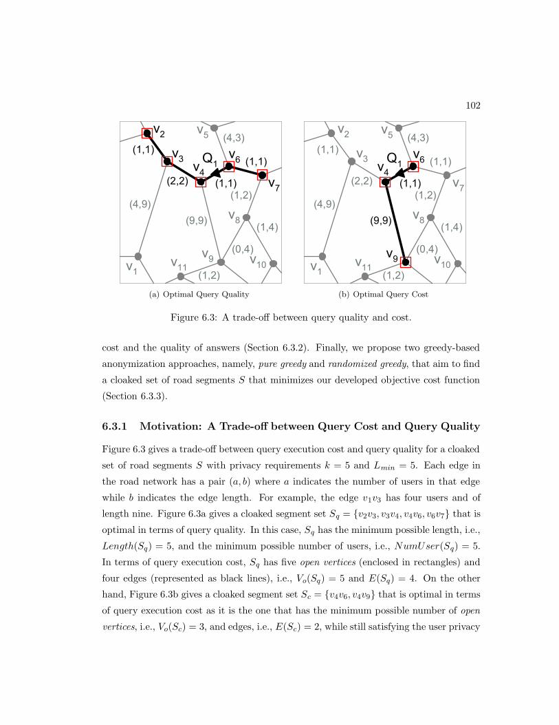
102

��

��

��

��

�

��

��

��

�

��

��

��

��

��

��

��

��

� ��

��

��

��

��

(a) Optimal Query Quality

��

��

��

��

�

��

��

��

�

��

��

��

��

��

��

��

��

� ��

��

��

��

��

(b) Optimal Query Cost

Figure 6.3: A trade-off between query quality and cost.

cost and the quality of answers (Section 6.3.2). Finally, we propose two greedy-based

anonymization approaches, namely, pure greedy and randomized greedy, that aim to find

a cloaked set of road segments S that minimizes our developed objective cost function

(Section 6.3.3).

6.3.1 Motivation: A Trade-off between Query Cost and Query Quality

Figure 6.3 gives a trade-off between query execution cost and query quality for a cloaked

set of road segments S with privacy requirements k = 5 and Lmin = 5. Each edge in

the road network has a pair (a, b) where a indicates the number of users in that edge

while b indicates the edge length. For example, the edge v1v3 has four users and of

length nine. Figure 6.3a gives a cloaked segment set Sq = {v2v3, v3v4, v4v6, v6v7} that is

optimal in terms of query quality. In this case, Sq has the minimum possible length, i.e.,

Length(Sq) = 5, and the minimum possible number of users, i.e., NumUser(Sq) = 5.

In terms of query execution cost, Sq has five open vertices (enclosed in rectangles) and

four edges (represented as black lines), i.e., Vo(Sq) = 5 and E(Sq) = 4. On the other

hand, Figure 6.3b gives a cloaked segment set Sc = {v4v6, v4v9} that is optimal in terms

of query execution cost as it is the one that has the minimum possible number of open

vertices, i.e., Vo(Sc) = 3, and edges, i.e., E(Sc) = 2, while still satisfying the user privacy

103

requirements. However, Sc may result in very bad answer quality Sc is 10 which is way

above the minimum length l privacy requirement.

From these examples, we can see that trying to find the optimal Sq, i.e., maximizing

the query quality, results in having five open vertices and four edges (Figure 6.3a) which

is 66.7% and 100% worse than what we can get from Sc (Figure 6.3b). On the other

hand, trying to find the optimal Sc that gives the minimal query execution cost, i.e., the

minimum possible number of open vertices and edges, results in the total segment length

of 10 (Figure 6.3b) which is 100% worse than what we can get from Sq (Figure 6.3a).

This raises the issue of finding an objective cost function that balances between query

execution cost and query quality.

6.3.2 Objective Cost Function

As we have discussed in the previous section, we need an objective cost function that

balances between query execution cost and query quality. The query execution cost is

measured by the cost models described in Section 6.2. On the other hand, the query

quality is measured by the number of candidate target objects returned by a database

server given that the query location is within a cloaked set of road segments S. In

general, the number of candidate target objects is proportional to the total length of

the road segments in S. Thus, the objective cost function aims to find a cloaked segment

set S, such that S not only satisfies the user privacy requirements, but it also minimizes

the query execution cost and the total segment length.

Based on these contradicting requirements, we distinguish between two cases for the

objective cost function based on whether the privacy requirements are achieved or not.

If the privacy requirements are not yet met, we try to minimize the query execution

cost while maximizing the number of users and total length of the road segments in S

as this will increase the query quality. On the other hand, if only one of the privacy

requirement is already met, we attempt to minimize the query execution cost and the

total length of S as further increase of the total length of S will unnecessarily degrade

the answer quality. Notice that in the second case, if k-anonymity privacy requirement

is already met, we do not have to worry about the number of users in S as maximizing or

minimizing the number of users will not affect the query quality. Then, we will discuss

the incorporation of each privacy requirement in our proposed objective cost function.

104

For the k-anonymity privacy requirement, when this requirement is not yet met, we

should select some edges that contain more users to S. For example, if adding edge ei or

ej to S incurs the same query execution cost QCost(S) that is computed by using the

cost models described in Section 6.2, the objective cost function should give a smaller

value to the edge containing more users; and thus, the objective cost function adjusts

QCost(S) by dividing it by a quality factor NumUser(S)/k. On the other hand, when

the k-anonymity requirement is satisfied, the number of users in S does not affect the

quality of answers, so the objective cost function no longer considers the k-anonymity

privacy requirement.

For the minimum length Lmin privacy requirement, if this requirement is not yet

achieved, we should select some longer edges to S. Similar to the k-anonymity privacy

requirement, the objective cost function adjusts QCost(S) by dividing it by a quality

factor Length(S)/Lmin. On the other hand, if the minimum length privacy requirement

is satisfied, the objective cost function gives a larger value to longer edges, i.e., dividing

QCost(S) by another quality factor Lmin/Length(S).

Since the quality factors of these two privacy requirements are normalized to the cor-

responding privacy requirement, we can encapsulate them in our objective cost function.

Hence, the quality factor is:

Quality(S) = min

(NumUser(S)

k, 1

)×min

(Length(S)

L min,

Lmin

Length(S)

).

Therefore, for each edge ei, we consider a new potential cloaked set of road segments

S = S ∪ {ei}, and we calculate the objective cost Cost(S,Q) as:

Cost(S,Q) =QCost(S,Q)

Quality(S), where

QCost(S,Q) =

{CostPKNN(S,K), if Q is a K-NN query;

CostPRange(S, r), if Q is a range query.

6.3.3 Greedy Approaches

Trying to find the optimal set of cloaked road segments S that minimizes a certain cost

function would require an exhaustive search process. As the underlying application of

105

road network anonymization (e.g., location-based services) is a real-time application in

which it is crucial to efficiently process the anonymization and query processing in a

minimal time, we avoid trying to get an optimal set S. Instead, we use a greedy ap-

proach to minimize the objective cost function developed in Section 6.3.2. In particular,

we present two efficient greedy approaches, namely pure greedy and randomized greedy

approaches, that rely on the objective cost function designed for balancing a trade-off

between query execution cost and query quality.

Pure Greedy Approach

The idea of our greedy approach is to start from the road segment in which the querying

user is residing. If this road segment satisfies the user’s privacy requirements, we return

it to a location-based database server as the cloaked road segment S. Otherwise, we

check all adjacent road segments of S and greedily pick the road segment that minimizes

the objective cost function. We keep adding these adjacent road segments greedily to S

until S satisfies the user privacy requirements. As the objective cost function is heavily

dependent on the underlying query execution cost model, such approach may result in

different S for different query types.

Algorithm 5 depicts the pseudo code of the pure greedy approach of our query-

aware location anonymization algorithm. The algorithm has two input parameters, the

identifier of the user U who issues the query and the issued query Q. The algorithm

starts by initializing a cloaked set of road segments S with the edge e that includes

the user U (Line 3 in Algorithm 5). If the current S does not satisfy U ’s privacy

requirements, i.e., U.k and U.Lmin, we do the following three steps (Lines 4 to 8 in

Algorithm 5): (1) We construct the set R that consists of all road segments that are

adjacent to some road segment in S. (2) For each road segment ei ∈ R, we calculate the

objective cost to decide whether ei should be added to S for the input query Q based

on the objective cost function designed in Section 6.3.2. Then, we choose the best edge

as the one that minimizes the objective cost function should it have been added to S.

(3) We add that best edge to the current cloaked set of road segments S. We keep doing

these three steps until S satisfies U ’s privacy requirements, i.e., NumUser(S) ≥ U.k

and Length(S) ≥ U.Lmin. Finally, we return S as the cloaked segment set for the user

U . It is important to note that S does satisfy the user privacy requirements while it

106

Algorithm 5 A Greedy Approach

1: function Greedy (User U , Query Q)2: e← the road segment contains the user U3: S ← {e}4: while NumUser(S) < U.k or Length(S) < U.Lmin do5: R← All adjacent road segments of S6: BestEdge← argminei∈R (Cost(S ∪ ei, Q))7: S ← S ∪BestEdge8: end while9: return S

aims to minimize the query execution cost and maximize the query quality according

to our developed objective cost function.

Figure 6.4 gives an example to illustrate the greedy approach for the query-aware

location anonymization algorithm where the user issues a K-NN query Q1 where K = 3

while being five anonymous within a set of connected road segments with a total length

of at least five, i.e., k = 5 and Lmin = 5. For ease of comparison and discussion, we

use the same road network that was used in Figure 6.3. Although we show only part

of the road network, we assume that the whole road network has R = 100, 000 road

segments and T = 1, 000 target objects. Hence, according to the query cost model

developed in Section 6.2, we will need to search R/T × K = 300 edges for each open

vertex in a cloaked segment set S. Since edge v4v6 contains Q1, we initially set the

cloaked set of road segments S to {v4v6}, where vertices v4 and v6 are open vertices

that are enclosed in rectangles. As S cannot satisfy the user privacy requirements, i.e.,

NumUser(S) = 1 and Length(S) = 1, we compute the objective cost of the adjacent

edges of v4v6 and add the edge with the lowest cost to S. The cost of these adjacent edges

is Cost(S∪v5v6) = (3×300+2)/(min(5/5, 1)×min(4/5, 5/4)) = 902/(1×4/5) = 1127.5,

Cost(S∪v6v7) = 902/(2/5×2/5) = 5637.5, Cost(S∪v3v4) = 902/(3/5×3/5) = 2505.6,

and Cost(S∪v4v9) = 902/(1×5/10) = 1804. Since edge v5v6 has the smallest objective

cost, we add v5v6 to S (Figure 6.4a).

However, S = {v4v6, v5v6} satisfies only the k-anonymity requirement, i.e.,

NumUser(S) = 5 and Length(S) = 4, so we compute the objective cost of the ad-

jacent edges of the edges in S. The cost of these adjacent edges is Cost(S ∪ v6v7) =

(3 × 300 + 3)/(min(6/5, 1) ×min(5/5, 5/5)) = 903/(1 × 5/5) = 903, Cost(S ∪ v3v4) =

107

��

��

��

��

�

��

��

��

�

��

��

��

��

��

��

��

��

� ��

��

��

��

��

(a) Add v5v6 to S = {v4v6}

��

��

��

��

�

��

��

��

�

��

��

��

��

��

��

��

��

� ��

��

��

��

��

(b) Add v6v7 to S={v4v6, v5v6}

Figure 6.4: Example of the greedy approach.

(4 × 300 + 3)/(min(7/5, 1) ×min(6/5, 5/6)) = 1203/(1 × 5/6) = 1443.6, and Cost(S ∪v4v9) = (4 × 300 + 3)/(min(14/5, 1) × min(13/5, 5/13)) = 1203/(1 × 5/13) = 3127.8.

Since edge v6v7 has the smallest objective cost, we add v6v7 to S (Figure 6.4b). Finally,

S = {v4v6, v5v6, v6v7} satisfies the user privacy requirements, i.e., NumUser(S) = 6 ≥ k

and Length(S) = 5 ≥ Lmin, and there are three open vertices in S, i.e., v4, v5, and v7,

that are enclosed in rectangles. This example shows that the developed objective cost

function effectively balances between query execution cost and query quality, because

the cloaked segment set S has the maximal query Length(S) = l = 5, and the query

execution cost of S (i.e., cost of S (i.e., Vo(S) = 3 and E(S) = 3) is only slightly dete-

riorated compared to the optimal query cost (i.e., Vo(Sc) = 3 and E(Sc) = 2) given in

Section 6.3.1.

Randomized Greedy Approach

Although the greedy approach is simple and effective in terms of achieving privacy re-

quirements, minimizing query execution cost, and maximizing query quality, the greedy

approach is vulnerable to adversary attacks. Basically, we assume the worst case that

an adversary knows the number of users and length of each road segment, and the ad-

versary is able to crack the system to know or guess the used objective cost function.

108

Then, the adversary can know the road segment in which the user issuing the query

is residing through a reverse engineering process. For example, given a cloaked set of

road segments S, the adversary performs two main steps. (1) The adversary selects a

certain edge ei ∈ S, and then applies the revealed cost function in a greedy manner for

ei to compute another cloaked set of road segments S ′. (2) If there is an edge ej where

ej ∈ S′ and ej /∈ S, the adversary knows that the user is not in ei. The main idea is

that if the user is in ei, S′ should always be included in S, i.e., S ′ ⊆ S, before S ′ is

equal to S. The adversary can repeat these two steps for each edge in S for all possible

combinations of the user’s privacy requirements, i.e., k and Lmin. When the adversary

achieves a case that S ′ = S, it is likely that the user who issued the query is in ei.

The main reason of having such a privacy attack is that the greedy approach relies on

a deterministic cost function to determine a cloaked set of road segments S. To this end,

we propose a randomized greedy approach for our query-aware location anonymization

algorithm. The idea is to inject some randomness into the process of selecting road seg-

ments to S. Rather than solely relying on a greedy approach, we will alternate between

greedy and random approaches. Although injecting randomness into the anonymization

process may degrade the query processing performance, i.e., query execution cost and

query quality, but it significantly reduces, if not prevent, the possibility of the adversary

attack. To balance between the query processing performance and the vulnerability of

adversary attacks, we introduce a user parameter, random factor (RandF ), that controls

the level of randomness injected into the greedy approach. When RandF is set to 0, our

randomized greedy approach acts exactly as the pure greedy approach. On the other

hand, when RandF is set to 1, our randomized greedy approach acts in a purely random

way where we keep randomly selecting the adjacent edges of a current cloaked segment

set S until S satisfies the user privacy requirements. In general, a larger RandF provides

more secure privacy for the user, yet it results in lower query processing performance. It

is important to note that both the pure greedy and randomized greedy approaches are

guaranteed to generate a cloaked set of road segments satisfying both the k-anonymity

and minimum length Lmin privacy requirements.

Algorithm 6 gives the pseudo code of our randomized greedy approach. The pseudo

code is similar to that of the pure greedy approach in Algorithm 5 except for the part of

choosing an edge in the set of adjacent edges of S, R, to be added to the current cloaked

109

Algorithm 6 A Randomized Greedy Approach

1: function RandomizedGreedy (User U , Query Q, Float RandF )2: e← the road segment contains the user U3: S ← {e}4: while NumUser(S) < U.k or Length(S) < U.Lmin do5: R← All adjacent road segments of S6: RandN ← a random number between 0 and 1, i.e., [0, 1)7: if RandF > RandN then8: BestEdge← a road segment is randomly selected from R9: else

10: BestEdge← argminei∈R (Cost(S ∪ ei, Q))11: end if12: S ← S ∪BestEdge13: end while14: return S

set of road segments S (Lines 6 to 11 in Algorithm 6). Basically, the randomized greedy

approach has an option to randomly select road segments to S. Thus, we generate

a random number between 0 and 1. If the input parameter RandF is greater than

the generated random number, we opt to randomly select a road segment among the

ones stored in R, i.e., the adjacent road segments of S. On the other hand, if the

input parameter RandF is less than the generated random number, we use our greedy

approach to select the road segment from R that minimizes the objective cost function

described in Section 6.3.2. By injecting randomness to the anonymization process, we

can prevent the reverse engineering attack as an adversary cannot guess the generated

random numbers.

6.4 Shared Execution Paradigm

As a location-based database server is likely to receive a numerous number of concurrent

queries, processing these queries individually would pose a system bottleneck. To tackle

this scalability issue, we propose a shared execution paradigm that aims to minimize

the number of queries executed by the database server for a set of private queries. The

main idea is to maximize the number of common vertices and edges in the cloaked set of

road segments of a set of similar queries issued from nearby users. Two or more queries

110

��

��

��

��

�

��

��

��

�

��

��

��

��

��

��

��

��

� ��

��

��

��

��

�

(a) Non-shared execution

��

��

��

��

�

��

��

��

�

��

��

��

��

��

��

��

� ��

��

��

��

��

�

��

(b) Shared execution

Figure 6.5: Motivating example of shared execution.

are similar if they belong to the same query type and interested in the same target

object type. It is important to note that the proposed shared execution paradigm can

be incorporated into both the pure greedy and randomized greedy approaches for query-

aware location anonymization. In this section, we first give the motivation of the shared

execution paradigm, and then present the algorithm with a running example.

6.4.1 Motivation

Figure 6.5 depicts a motivating example of the proposed shared execution paradigm,

in which the location anonymizer receives three similar queries Q = {Q1, Q2, Q3} at

the same time. The privacy requirements of these queries are (Q1.k=5, Q1.Lmin=5),

(Q2.k=6, Q2.l=7), and (Q3.k=3, Q3.=6). Without the concept of shared execution,

we use the use the pure greedy approach to anonymize the location information of

these queries individually. Figure 6.4b gives the cloaked set of road segments S1 of

Q1, while the cloaked segment sets S2 and S3 of Q2 and Q3 are depicted in Fig-

ure 6.5a. Anonymizing these queries individually results in three cloaked segment sets

S1 = {v4v6, v5v6, v6v7}, S2 = {v1v3, v2v3, v3v4}, and S3 = {v6v7, v7v8, v8v10} that con-

tain a total of nine edges (represented as black lines) and ten open vertices (enclosed

in rectangles), i.e., {v4, v5, v7} in S1, {v1, v2, v4} in S2, and {v6, v7, v8, v10} in S3. Thus,

111

Algorithm 7 A Greedy Approach with Shared Execution

1: function SharedExecutionGreedy (QuerySet Q)2: S ← {∅}3: Sort Q by the query parameter in decreasing order4: for Each query Qi ∈ Q do5: e← the road segment contains the user Ui of Qi

6: Si ← {e}7: while NumUser(Si) < Ui.k or Length(Si) < Ui.Lmin do8: R← All adjacent road segments of Si

9: if R ∩ S is empty then10: e← argminej∈R (Cost(Si ∪ ej , Qi))11: else12: e← argmaxej∈{R∩S} (Quality(Si ∪ ej))13: end if14: Si ← Si ∪ e15: end while16: S ← S ∪ Si

17: end for18: return S

the database server has to retrieve the target objects of these nine edges and execute

the requested query at each of these ten open vertices.

With the proposed shared execution paradigm, the location anonymization algo-

rithm aims to maximize the number of common open vertices and edges of the cloaked

segment sets of a set of similar queries. Figure 6.5b depicts the set S of distinct

edges in the cloaked segment sets S1, S2, and S3 that are computed by the pure

greedy approach with our shared execution paradigm, in which S1 = {v4v6, v5v6, v6v7},S2 = {v3v4, v4v6, v5v6, v6v7}, and S3 = {v3v4, v4v6, v6v7, v7v8}. Hence, S contains five

distinct edges (represented as black lines), i.e., v3v4, v4v6, v5v6, v6v7, and v7v8, and five

distinct open vertices (enclosed in rectangles), i.e., v3, v4, v5, v7, and v8. This exam-

ple shows that the shared execution paradigm reduces the number of edges and open

vertices among the cloaked segment sets of the three queries by 44.4% (i.e., from nine

edges to E(S) = 5) and 50% (i.e., from ten open vertices to Vo(S) = 5), respectively.

As a result, the database server needs to retrieve the target objects of five edges and

execute the requested query at five open vertices, and then share the answer of these

queries among Q1, Q2, and Q3.

112

��

��

��

�

��

��

��

�

��

��

��

��

��

��

��

� ��

��

��

��

��

�

(a) Add v4v6 to S2

��

��

��

�

��

��

��

�

��

��

��

��

��

��

��

� ��

��

��

��

��

�

(b) Add v5v6 to S2

��

��

��

�

��

��

��

�

��

��

��

��

��

��

��

� ��

��

��

��

��

�

(c) Add v6v7 to S2

��

��

��

�

��

��

��

�

��

��

��

��

��

��

��

� ��

��

��

��

��

�

(d) Cloaked Set S3 of Q3

Figure 6.6: An example of the shared execution scheme for a query setQ = {Q1, Q2, Q3}.

6.4.2 Algorithm

Main idea. Given a set of n similar queries Q = {Q1, Q2, . . . , Qn} received by the

location anonymizer at the same time or within a short time interval, the shared exe-

cution paradigm aims to maximize the number of common open vertices and edges in

the cloaked segment sets S1, S2, . . . , Sn for the queries in Q. S is a set of distinct edges

in the cloaked segment sets S1, S2, . . . , Sn, i.e., S =⋃

1≤i≤n Si. The main idea is that

when we compute a cloaked set Si of a query Qi, we always give a higher priority to

select the edges that are in the set of adjacent edges of Si, R, and have been selected

113

by other preceding queries in Q to Si, i.e., these edges are in the set {R∩S}. The main

reason is that adding any edge from S will have a zero query execution cost because

the query execution cost of the edges in S is absorbed by other queries in Q. Thus,

by using the quality function described in Section 6.3.2, we add the edge that gives the

highest quality of answers among the set {R∩ S} to Si. However, in case that {R ∩ S}is empty, we simply employ our objective cost function to select the best candidate

edge to Si. Although the shared execution paradigm would incur longer anonymization

time for some queries, it improves the average anonymization time of the queries in the

similar query set, and this sacrifice will be paid off by the significant gain in the query

processing at the database server. Experimental results in Section 7.4 give more details

on this performance gain.

Algorithm. Algorithm 7 depicts the pseudo code of the shared execution paradigm

applied to the pure greedy approach (or the randomized greedy approach with the same

modifications). The input of the algorithm is a set of similar queries Q. We maintain

a set S to store the distinct edges in the cloaked set of road segments of each query

in Q. Initially, we set S to empty and sort the queries in Q by their parameters in

decreasing order, i.e., the value of K of K-NN queries or the network range distance r

of range queries (Lines 2 to 3 in Algorithm 7). The main idea behind this sorting is to

ensure that the answer of the requested query at a selected open vertex can be used by

a database server to answer the subsequent queries in Q. For example, a K-NN query

answer can be used to answer another K′-NN query if K ≥ K′. For each query Qi in Q,

the proposed shared execution paradigm is applied to the pure greedy approach (or the

randomized greedy approach) to find a cloaked set of road segments Si. First, we set

the edge that contains the querying user Ui to Si (Line 6 in Algorithm 7). If Si does

not satisfy the user privacy requirements, i.e., Ui.k and Ui.Lmin, we repeatedly select

the adjacent edges of Si, R, to Si until Si satisfies the user privacy requirements. We

distinguish between two cases of selecting the best edge to Si. Case 1: {R∩S} is empty.

In this case, there is no adjacent edge of Si in S. Thus, we simply use the objective cost

function to select an edge with the best cost among the set of adjacent edges of Si, R

(Line 10 in Algorithm 7). Case 2: {R ∩ S} is not empty. In this case, there are some

adjacent edges of Si are in S. We select an edge with the largest quality from the set

{R ∩ S} (Line 12 in Algorithm 7). It is important to note that choosing any edge from

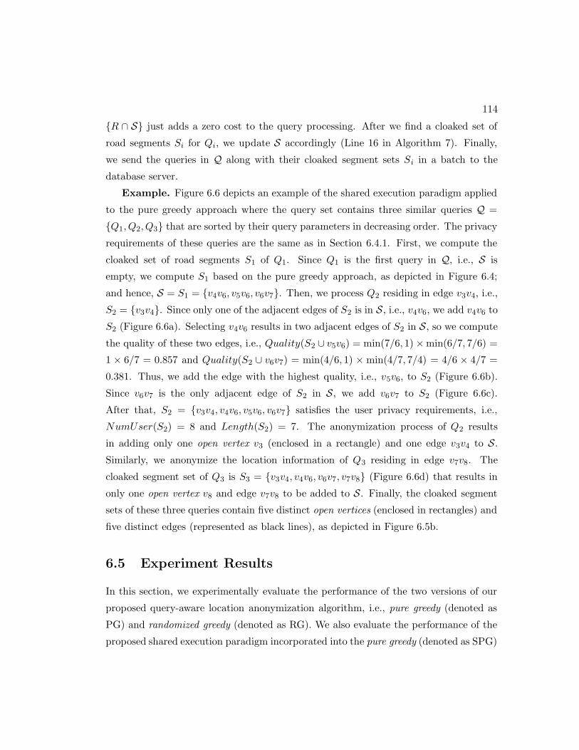
114

{R ∩ S} just adds a zero cost to the query processing. After we find a cloaked set of

road segments Si for Qi, we update S accordingly (Line 16 in Algorithm 7). Finally,

we send the queries in Q along with their cloaked segment sets Si in a batch to the

database server.

Example. Figure 6.6 depicts an example of the shared execution paradigm applied

to the pure greedy approach where the query set contains three similar queries Q =

{Q1, Q2, Q3} that are sorted by their query parameters in decreasing order. The privacy

requirements of these queries are the same as in Section 6.4.1. First, we compute the

cloaked set of road segments S1 of Q1. Since Q1 is the first query in Q, i.e., S is

empty, we compute S1 based on the pure greedy approach, as depicted in Figure 6.4;

and hence, S = S1 = {v4v6, v5v6, v6v7}. Then, we process Q2 residing in edge v3v4, i.e.,

S2 = {v3v4}. Since only one of the adjacent edges of S2 is in S, i.e., v4v6, we add v4v6 to

S2 (Figure 6.6a). Selecting v4v6 results in two adjacent edges of S2 in S, so we compute

the quality of these two edges, i.e., Quality(S2 ∪ v5v6) = min(7/6, 1)×min(6/7, 7/6) =

1 × 6/7 = 0.857 and Quality(S2 ∪ v6v7) = min(4/6, 1) ×min(4/7, 7/4) = 4/6 × 4/7 =

0.381. Thus, we add the edge with the highest quality, i.e., v5v6, to S2 (Figure 6.6b).

Since v6v7 is the only adjacent edge of S2 in S, we add v6v7 to S2 (Figure 6.6c).

After that, S2 = {v3v4, v4v6, v5v6, v6v7} satisfies the user privacy requirements, i.e.,

NumUser(S2) = 8 and Length(S2) = 7. The anonymization process of Q2 results

in adding only one open vertex v3 (enclosed in a rectangle) and one edge v3v4 to S.

Similarly, we anonymize the location information of Q3 residing in edge v7v8. The

cloaked segment set of Q3 is S3 = {v3v4, v4v6, v6v7, v7v8} (Figure 6.6d) that results in

only one open vertex v8 and edge v7v8 to be added to S. Finally, the cloaked segment

sets of these three queries contain five distinct open vertices (enclosed in rectangles) and

five distinct edges (represented as black lines), as depicted in Figure 6.5b.


In this section, we experimentally evaluate the performance of the two versions of our

proposed query-aware location anonymization algorithm, i.e., pure greedy (denoted as

PG) and randomized greedy (denoted as RG). We also evaluate the performance of the

proposed shared execution paradigm incorporated into the pure greedy (denoted as SPG)

115


Parameter Default Value Range

Number of users 100K 100K - 500KNumber of queries 5K 2K - 10K

Anonymity levels (k) 200 100 - 500Min. total segment length (Lmin) 10× l, l = 1590.6 10 × l - 50× l

Random factor RandF 0.2 0.1 - 0.5Requested no. of objects K 10 1 - 20Required range distance r 10× l 5× l - 30× l

and randomized greedy (denoted as SRG) approaches.

Baseline approach. We compare our approaches with the closest work [100] (de-

noted as BL) that is the only related work considering location anonymization and

privacy-preserving query processing in road networks. However, this work uses the

Casper’s location anonymization algorithm [12] that is designed for the Euclidean space

to blur users’ locations into k-anonymous spatial regions. After determining a cloaked

spatial region, the set of road segments intersecting the spatial region forms a cloaked

segment set.

Experiment settings. We use a network-based generator [88] to generate moving

objects on an actual road map that has 57,020 edges and 42,135 vertices in which the

average length of the edges (l) is 1,590.6 and the the average degree of connectivity

of the vertices (d) is 2.7. At the database server, we employ an incremental network

expansion algorithm [103] and a depth-first search algorithm to process K-NN and range

queries in the road network, respectively. We evaluate our algorithms with respect to

two performance measures, CPU time and total segment length. The CPU time is the

sum of the average time consumed in the anonymization process (i.e., cloaking time)

and the average query processing time at the database server. The total segment length

is the sum of the length of all road segments in a cloaked segment set S, Length(S).

Since a cloaked segment set with a larger total segment length is more likely to give a

larger candidate answer set, this measure indicates the query quality of S.

Parameter settings. Unless mentioned otherwise, the experiments in this section

consider 100,000 mobile users and 500 target objects in the road network in which

116

��

��

��

��

��

��

��

��

��

��

��

��

��

��

��

�

�

�

�

��

��

��

�� !�

��"��#��

�$��%�#��

(a) CPU Time

�

��

��

��

��

��

��

��

!

"!

#�

(b) Total Segment Length

Figure 6.7: Number of mobile users (K-NN queries).

5,000 users issue queries at each time interval. The default user privacy requirements,

anonymity level k and minimum length (Lmin), are k = 200 and Lmin = 10 × l, where

l is the average length of the road segments in the road network. The random factor

RandF for our randomized greedy approach is set to 0.2. The query parameters of

K-NN and range queries are K = 10 and r = 10 × l, respectively. Table 6.1 gives a

summary of the parameter settings.

6.5.1 Scalability

Figures 7.8a and 7.8b depict the scalability of our pure greedy (PG) and randomized

greedy (RG) approaches with respect to increasing the number of users from 100K to

500K for K-NN queries in terms of two performance measures, the average CPU time

per query (Figure 7.8a) and average total segment length per cloaked segment set S

(Figure 7.8b). Figure 7.8a gives the overall CPU time which includes the location

anonymization time at the location anonymizer (represented by shaded bars) and the

query processing time at the database server (represented by white bars). Focusing

on the baseline algorithm (BL), although it has better anonymization time than our

proposed greedy approaches, it suffers from bad query processing performance and low

quality of answers. The main reason is that BL always generates cloaked segment

sets with a larger number of open vertices and larger total segment length than our

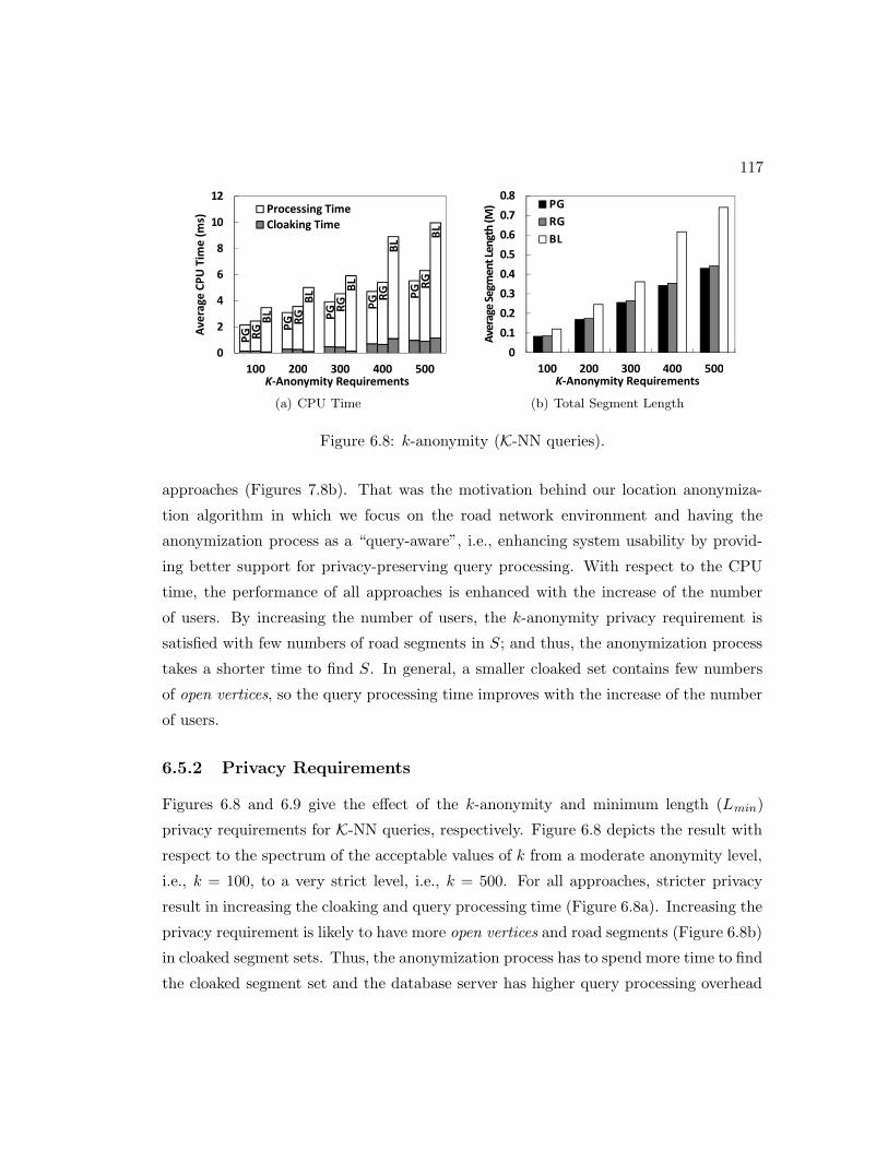
117

��

��

��

��

��

��

��

��

��

�

�

�

��

��

��

��

��

�� ! ��"#�� !�

��$��

�%��&��

(a) CPU Time

�

��

��

��

��

��

��

��

��

��

��

��

�� !�� "

#$

�$

%�


Figure 6.8: k-anonymity (K-NN queries).

approaches (Figures 7.8b). That was the motivation behind our location anonymiza-

tion algorithm in which we focus on the road network environment and having the

anonymization process as a “query-aware”, i.e., enhancing system usability by provid-

ing better support for privacy-preserving query processing. With respect to the CPU

time, the performance of all approaches is enhanced with the increase of the number

of users. By increasing the number of users, the k-anonymity privacy requirement is

satisfied with few numbers of road segments in S; and thus, the anonymization process

takes a shorter time to find S. In general, a smaller cloaked set contains few numbers

of open vertices, so the query processing time improves with the increase of the number

of users.

6.5.2 Privacy Requirements

Figures 6.8 and 6.9 give the effect of the k-anonymity and minimum length (Lmin)

privacy requirements for K-NN queries, respectively. Figure 6.8 depicts the result with

respect to the spectrum of the acceptable values of k from a moderate anonymity level,

i.e., k = 100, to a very strict level, i.e., k = 500. For all approaches, stricter privacy

result in increasing the cloaking and query processing time (Figure 6.8a). Increasing the

privacy requirement is likely to have more open vertices and road segments (Figure 6.8b)

in cloaked segment sets. Thus, the anonymization process has to spend more time to find

the cloaked segment set and the database server has higher query processing overhead

118

��

��

��

��

��

��

��

��

�

�

�

��

� ��

��

� ��

��!"��

�#!�$��

(a) CPU Time

�

��

��

��

��

��

��

��

��

��

� ��

�

�

!�


Figure 6.9: Minimum length Lmin (K-NN queries).

to compute the candidate answer set. With a higher anonymity level, the improvement

of our approaches (i.e., PG and RG) over the baseline algorithm (BL) significantly

increases in both the CPU time and query quality.

Figure 6.9 gives the performance of our approaches with respect to varying the

minimum length privacy requirement from Lmin = 10 × l to 50 × l, where l is the

average length of the segments in the road network. Similar to the k-anonymity privacy

requirement, the cloaking and processing time increases as the value of l gets larger.

Our greedy-based approaches also perform better than the baseline algorithm (BL) in

terms of both the CPU time (Figure 6.9a) and query quality (Figure 6.9b) when the

user specifies a stricter minimum length privacy requirement.

6.5.3 Query Parameters

Figures 6.10a and 6.10b give the performance of our greedy-based approaches, PG

and RG, for various query parameters of K-NN and range queries (r) in terms of the

CPU time, respectively. Figures 6.10a and 6.10b give the CPU time of all approaches

with respect to varying the value of K of K-NN queries from 1 to 20 and the network

range distance r of range queries from 5× l to 30× l, respectively. With a larger query

parameter, the query processing time increases as the database server needs to spend

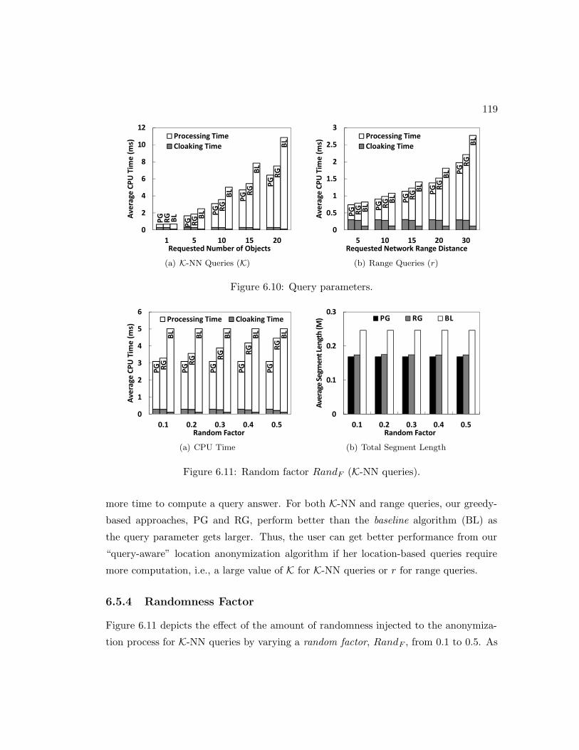
119

��

��

��

��

��

��

��

��

��

��

��

��

��

��

�

�

�

��

��

� � ��

��

��

�� !��"#�$ !%�&��

��"&��'��

�("�)�'��

(a) K-NN Queries (K)

��

��

��

��

��

��

��

��

��

��

��

��

�

��

��

��

�

� � � � ��

� ��

��

�� !�"��#��$��#%�

��!%��#��

�&!�"�#��

(b) Range Queries (r)

Figure 6.10: Query parameters.

��

��

��

��

��

��

��

��

��

��

�

�

�

�

�

� � � � � � � �

��

��

�� !"��

��!�� #��$��

(a) CPU Time

�

��

��

��

��

��

��

��

��


Figure 6.11: Random factor RandF (K-NN queries).

more time to compute a query answer. For both K-NN and range queries, our greedy-

based approaches, PG and RG, perform better than the baseline algorithm (BL) as

the query parameter gets larger. Thus, the user can get better performance from our

“query-aware” location anonymization algorithm if her location-based queries require

more computation, i.e., a large value of K for K-NN queries or r for range queries.

6.5.4 Randomness Factor

Figure 6.11 depicts the effect of the amount of randomness injected to the anonymiza-

tion process for K-NN queries by varying a random factor, RandF , from 0.1 to 0.5. As

120

��

��

��

��

��

��

��

��

��

��

��

��

��

��

��

��

��

��

��

��

�

�

�

�

� � � �

��

��

�� !�

��"��#��

�$��%�#��

(a) Number of Users

��

��

��

��

��

��

��

��

��

��

��

��

��

��

��

��

��

��

��

��

�

�

�

�

�

�

�

�

� � � �

��

��

��!�!"� �"��#$�� !�

��%��!��

�&��'�!��

(b) k-Anonymity

Figure 6.12: Objective cost function (K-NN queries).

a reference, we plot the result of the pure greedy approach (PG) and baseline algorithm

(BL), though they are not affected by the random factor. The cloaking time of the

randomized greedy approach (RG) gets better with more injected randomness, i.e., a

larger RandF . The main reason for this is that increasing the randomness alleviates

the need for the more expensive computation of the best edge (i.e., the objective cost

function) to be added to a cloaked segment set S. However, injecting randomness to

the anonymization process degrades query processing performance and query quality,

as depicted in Figures 6.11a and 6.11b, respectively. Since injecting more randomness

into the anonymization process only slightly increases the total segment length (Fig-

ure 6.11b), the main reason of the query performance deterioration is due to a larger

number of open vertices in the cloaked segment sets. Thus, we should limit the random

factor such that we can have moderate sacrifice of query processing performance in order

to obtain more secure privacy.

6.5.5 Objective Cost Function

Figure 6.12 depicts the effectiveness of our objective cost function described in Sec-

tion 6.3.2 with respect to increasing the number of users from 100K to 500K (Fig-

ure 6.12a) and the k-anonymity privacy requirement from k = 100 to 500 (Figure 6.12b)

for K-NN queries. To evaluate the objective cost function used by the pure greedy (PG)

and randomized greedy (RG) approaches, we compare them with the pure greedy and

121

��

��

��

��

��

��

��

��

��

��

��

��

��

��

��

��

��

��

��

��

�

�

�

�

��

� ��

��

��

��!��"�� #��$�"��

(a) K-NN Queries

��

��

��

��

��

��

��

��

��

��

��

��

��

��

��

��

��

��

��

�

��

��

��

��

�

��

��

� ��

��

��

��!��"�� #��$�"��

(b) Range Queries

Figure 6.13: Number of queries.

randomized greedy approaches that rely solely on the query execution cost model de-

scribed in Section 6.2 (denoted as PG-QCost and RG-QCost, respectively). The results

show that our objective cost function consistently performs better than the greedy ap-

proaches based on the query execution cost model. However, the cloaking time of the

greedy approaches using our objective cost function PG and RG is worse than the PG-

QCost and RG-QCost approaches. The main reason for this is that our objective cost

function incurs higher computational overhead than the query execution cost model.

By using our objective cost function, i.e., PG and RG approaches, the cloaked segment

set results in lower query processing cost that pays off the computational overhead of

the anonymization process. Furthermore, when we need to find a cloaked segment set

with more road segments, i.e., in a case of fewer numbers of users (Figure 6.12a) or

stricter privacy requirements (Figure 6.12b), the objective cost function is clearly more

effective than using only the query execution cost model.

6.5.6 Shared Execution Paradigm

In this section, we evaluate the performance of the shared execution paradigm incorpo-

rated into the pure greedy (denoted as SPG) and randomized greedy (denoted as SRG)

approaches with respect to workload, privacy requirements, and query parameters for

both K-NN and range queries.

122

��

��

��

��

��

��

��

��

��

��

��

��

��

��

��

��

��

��

��

��

�

�

�

�

�

�

��

��

��

�� !"��

��#��

�$��%��

(a) k-Anonymity

��

��

��

��

��

��

��

��

��

��

��

��

��

��

��

��

��

��

��

�

�

�

�

��

��

��

� ��

��!" ��

�#!�$��

(b) Minimum Length (Lmin)

Figure 6.14: Privacy requirements (K-NN queries).

Workload. Figure 6.13 depicts the effect of the query workload on the shared

execution approaches, SPG and SRG, by varying the number of queries received by the

location anonymizer within a short time period from 2K to 10K. Since the non-shared

execution approaches, PG and RG, process the queries individually, their performance

is not affected by varying the workload. On the other hand, the query processing cost of

the shared execution approaches significantly reduces as the workload increases. This is

because when the workload increases, it is likely to have more nearby similar queries; and

thus, there are more common open vertices and edges in their cloaked segment sets. The

results clearly indicate that our proposed shared execution paradigm effectively improves

system scalability, especially when the system encounters a high query workload.

Privacy requirements. Figures 6.14a and 6.14b give the performance of the shared

execution approaches with respect to increasing the anonymity levels from k = 100 to

500 and the minimum length requirement from Lmin = 10 × l to 50 × l for K-NN

queries, respectively. When the privacy requirement gets stricter, the anonymization

process spends more time to find cloaked segment sets; and hence, the cloaking time

of all approaches increases. For non-shared execution approaches, PG and RG, the

query processing time increases as the privacy requirement gets stricter. Increasing the

privacy requirement results in cloaked segment sets with more road segments. Since

these cloaked segment sets are likely to contain more open vertices and road segments,

the query processing cost increases. On the other hand, it is interesting to see that

123

��

��

��

��

��

��

��

��

��

��

��

��

��

��

��

��

��

��

�

�

�

�

�

�

� ��

��

��

�� !�� "��#$�% "&�'��

��#'��(��

�)#�*�(��

(a) K-NN Queries (K)

��

��

��

��

��

��

��

��

��

��

��

��

��

��

��

��

��

��

��

��

�

��

�

��

��

� ��

��

��

� �� !��"� �#��"$

�� $ ��"��

�% �!�"��

(b) Range Queries (r)

Figure 6.15: Query parameters.

the query processing cost of the shared execution approaches, SPG and SRG, slightly

improves as the privacy requirement gets stricter. The main reason for this is that it

is likely to have more common open vertices and edges of a set of similar queries, when

their cloaked segment sets incur more road segments.

Query parameters. Figure 6.15 depicts the effect of query parameters on the

performance of the shared execution approaches, SPG and SRG, with respect to varying

the requested number of nearest target objects (K) of K-NN queries from 1 to 20 and the

requested network range distance (r) of range queries from 5× l to 30 × l. Since these

two query parameters do not influence the anonymization process, the cloaking time

of all approaches is not affected. As discussed in Section 6.5.3, the query processing

time of all approaches increases when the query parameter gets larger. The results

show that the shared execution approaches clearly perform better than the non-shared

execution approaches in terms of the query processing time as the query parameters

get larger. This is because it is likely to have more common open vertices and edges in

larger cloaked segment sets. The results indicate that our shared execution paradigm

is more effective to enhance system scalability when the issued location-based queries

require more computation.

124

6.6 Summary

This chapter presents a query-aware location anonymization algorithm for road net-

works. The proposed algorithm distinguishes itself from all previous location anonymiza-

tion algorithms in the sense that it is query-aware and is designed specifically for the

road network environment. The proposed query-aware location anonymization algo-

rithm aims to blur a user location on a road network into a set of connected road

segments S such that: (a) there exist at least k users in S, and the total segment length

of the road segments in S is at least Lmin, (b) the processing cost of the requested

query over S is minimized, and (c) the query quality of S is maximized. Based on a

developed objective cost function that takes into account privacy requirements, query

processing cost, and query quality, we propose two greedy-based approaches for location

anonymization in road networks. To accommodate intervals with a high workload, we

also propose a shared execution paradigm to improve the scalability of our anonymiza-

tion process to support larger numbers of quires in a short time period. Extensive

experimental results show that our proposed location anonymization algorithm with

the two proposed approaches is efficient and scalable while preserving users’ location

privacy and enabling high quality services through minimizing the developed objective

cost function. The results also indicate that the shared execution paradigm significantly

improves system scalability and query processing performance.

Chapter 7

Location Anonymization in

Peer-to-Peer Environments

In this chapter, we extend the location anonymization functionality of the Casper system

in mobile peer-to-peer (P2P) environments. A mobile P2P network is a highly ad-hoc

environment in which mobile users can only communicate with other peers through

multi-hop routing without any support of fixed communication infrastructure or cen-

tralized/distributed servers. There are many unique limitations in the mobile P2P

environment, e.g., user mobility, limited transmission range, multi-hop communication,

scarce communication resources, and network partitions1 . In terms of system archi-

tecture, existing spatial cloaking techniques can be classified into three main categories,

centralized (e.g., [32, 36, 37, 44, 12, 47, 48]), distributed (e.g., [38, 39]), and peer-to-

peer approaches (e.g., [19]). Since the spatial cloaking algorithms proposed for the

centralized or distributed approach rely on fixed communication infrastructure and cen-

tralized/distributed servers, they cannot be applied to the mobile P2P environment. To

our best knowledge, our previous work is the only spatial cloaking algorithm for the

mobile P2P environment [19]. The main idea of the P2P spatial cloaking algorithm is

that when a mobile user wants to obtain services from an LBS provider, she collabo-

rates with other peers via multi-hop communication to blur her location into a cloaked

area. Our algorithm guarantees that the cloaked area satisfies the user’s k-anonymity

1 In a partitioned network, mobile users are partitioned into disjoint networks, in which a mobileuser is only able to communicate with other peers residing in her network partition.

125

126

and minimum area Amin privacy requirements. Then, the user sends her location-based

query along with the cloaked area to the LBS provider to obtain her desired services.

Since the location-based database server does not know the exact user location, it can

only return an answer set that includes the exact answer to the user. Thus, after the

user gets the answer set from the database server, she has to compute the exact answer

from the answer set.

In this chapter, we propose three key features to enhance the scalability, efficacy

and privacy protection of our P2P spatial cloaking algorithm. Since the mobile P2P

environment has limited communication resources and constrained transmission range,

excessively searching the network for peers would pose a scalability issue. To this

end, we propose an information sharing scheme for our P2P spatial cloaking algorithm

to enable mobile users to share their gathered peer location information with nearby

peers. If the mobile user can get enough peer location information from a peer, she

does not need to search the network; and therefore, the information sharing scheme can

reduce communication overhead. In addition, the mobile user may encounter a network

partition problem in the mobile P2P environment, i.e., the number of users residing

in her network partition is less than her required anonymity level, i.e., k, she cannot

find enough peer location information to satisfy her k-anonymity privacy requirement.

To alleviate the network partition problem, we design a historical location scheme that

allows users to utilize the peer location information cached by the peers residing in

their network partition. We use a consecutive approach to adjust such stale location

information to capture its uncertainty. Furthermore, the mobile user needs to search

the network for an adequate number of peers to satisfy her required anonymity level.

Since the peer search process usually starts at the user and spreads out from her nearby

peers to farther peers, the user may be close to the center of the cloaked area. Thus,

an adversary could guess that the user who is the closest to the center of a cloaked area

is the actual query issuer, i.e., a “center-of-cloaked-area” privacy attack. To avoid such

a privacy breach, we propose a cloaked area adjustment scheme that adjusts a cloaked

area such that the probability of the actual query issuer being the closest to the center

of a cloaked area is 1/K.

We evaluate the performance of our proposed features through simulated experi-

ments. The experimental results show that these features enhance the scalability of our

127

��

��

��

��

��

��

��

��

��

��

Figure 7.1: System architecture.

P2P spatial cloaking algorithm while guaranteeing the user’s location privacy protection.

In general, the contributions of this chapter can be summarized as follows:

• We propose a spatial cloaking algorithm for mobile peer-to-peer environments.

(Section 7.2.1)

• We introduce an information sharing scheme for our spatial cloaking algorithm to

enable mobile users to share their gathered peer location information with other

peers in order to reduce communication overhead. (Section 7.2.2)

• We design a historical location scheme for our algorithm to overcome the network

partition problem. (Section 7.2.3)

• We propose a cloaked area adjustment scheme for our algorithm to avoid the

“center-of-cloaked-area” privacy attack. (Section 7.2.4)

• We experimentally evaluate our P2P spatial cloaking algorithm with the three en-

hancement schemes. The experimental results show that the enhanced algorithm

is scalable while guaranteeing the user’s location privacy protection. (Section 7.4)

7.1 System Model

Figure 7.1 depicts the system architecture of our peer-to-peer (P2P) spatial cloaking

algorithm that consists of two entities, mobile users and location-based database servers.

128

We will first discuss our privacy threat model and privacy settings in user privacy

profiles, and then describe each entity in our system.

Privacy threat model. We assume that mobile users are trusted, so they do not

use their gathered peer location information to attack our system. However, we do not

have any assumption about the trustworthiness of the location-based service providers.

Thus, we assume that an adversary can utilize the information gathered by the service

provider to make privacy attacks. In addition, we only focus on snapshot location-based

queries, and each query is assigned a unique pseudonymous identity that is completely

unrelated to the user’s personal identity in order to ensure the pseudonymity of the

user’s location information [9].

User privacy profiles. Each user specifies her privacy requirements in a privacy

profile in a form of (K,Amin), where k indicates the required anonymity level and Amin

indicates the required minimum area of her cloaked areas. In other words, the user

wants to find a cloaked area that includes at least k users and has an area of at least

Amin. Amin is particularly useful in a dense area where a large k would not achieve

high privacy protection. For example, a user in a stadium with K = 100 may result in

a very small cloaked area. It is important to note that the user can change her privacy

profile at any time to guarantee that her specified privacy settings achieve her desired

privacy protection in different situations.

The privacy profile can be extended to support temporal, spatial, and/or interde-

pendent constraints on the required anonymity level and the required cloaked area size.

• Temporal constraint. The user can specify her privacy requirements for different

time intervals. For example, a user is willing to reveal her location information dur-

ing office hours, e.g., (K = 1, Amin = 0 mile) between 8:00 AM and 5:00 PM, but

she needs high privacy protection after office hours, e.g., (K = 100, Amin = 5 miles)

after 5:00 PM.

• Spatial constraint. The user can specify her privacy requirements for differ-

ent geographic regions. For example, a user needs a small Amin in downtown

areas, e.g., (K = 50, Amin = 1 mile), but a large Amin in rural areas, e.g.,

(K = 50, Amin = 10 miles). This is because a high density of geographic fea-

tures in a downtown area can make the adversary very difficult to infer anything

129

about the user even a small cloaked area of a couple of city blocks.

• Interdependent constraint. The user can specify an interdependence between the

anonymity level and the size of a cloaked area. For example, a user can specify a

maximum area Amax requirement of her cloaked areas, i.e., she is happy with a

cloaked area of a size Amax regardless of the number of users within the cloaked

area. Amax also ensures the query utility of our spatial cloaking algorithm.

Since it is straightforward to extend our P2P spatial cloaking algorithm to support

temporal, spatial, and/or interdependent constraints, we only discuss how our algorithm

finds cloaked areas satisfying both k and Amin in this paper.

Mobile users. Each mobile user is equipped with two wireless network interface

cards; one of them is dedicated to connect to a mobile base station to communicate

with location-based database servers, while the other one is devoted to communicate

with other peers via multi-hop routing without any support of fixed communication

infrastructure or centralized/distributed servers. This multi-interface approach has been

adopted in location-based services (e.g., [19, 105]) and mobile peer-to-peer information

access applications (e.g., [106, 107]). Each user is also equipped with a positioning

device, e.g., GPS, to determine her location that is represented as a coordinate (x, y).

It is important to note that we do not have any assumption about the transmission

range of the user mobile device, i.e., the mobile users can have different transmission

ranges, and the network topology.

Location-based database servers. A privacy-aware query processor embedded

inside the location-based database server has the ability to deal with location-based

queries with cloaked areas. When a mobile user wants to obtain services from a location-

based service provider, she executes our P2P spatial cloaking algorithm to blur her

location into a cloaked area that satisfies her privacy requirements. Then, the user

sends her location-based query along with the cloaked area to the database server.

Since the query processor does not know the exact user location, it can only compute

an answer set that includes the exact answer to the user. Then, the database server

sends the answer set to the user, and the user computes the exact answer from the

answer set.

130

7.2 Peer-to-Peer Spatial Cloaking Algorithm

We now present our spatial cloaking algorithm in mobile peer-to-peer (P2P) environ-

ments where no fixed communication infrastructure or centralize/distributed servers are

available. Thus, the mobile users are only able to collaborate with each other through

multi-hop routing to execute our algorithm. Such a highly ad-hoc mobile network poses

many limitations to the computing environment, e.g., user mobility, limited transmis-

sion range, multi-hop communication, scarce communication resources, and network

partition problems. In this section, we first describe our P2P spatial cloaking algorithm

(Section 7.2.1). Then, we present the three key features proposed for our algorithm.

Section 7.2.2 describes the information sharing scheme that enables users to share their

gathered peer location information with nearby peers in order to reduce communication

overhead. Section 7.2.3 gives the historical location scheme that allows users to utilize

stale peer location information to alleviate the network partition problem. Section 7.2.4

presents the cloaked area adjustment scheme that guarantees our algorithm to be free

from the “center-of-cloaked-area” privacy attack. We start by assuming that the net-

work partition problem does not take place, i.e., all mobile users can communicate with

each other through multi-hop routing in the network. The network partition problem

will be addressed in Section 7.2.3.

7.2.1 Spatial Cloaking Algorithm

The basic idea of our P2P spatial cloaking algorithm is that a mobile user communicates

with other peers via multi-hop routing to find at least K − 1 peers. Then, the user

determines a cloaked area that includes the K − 1 nearest peers and herself. The

cloaked area is k-anonymous because the user is indistinguishable among k users within

the cloaked area. After satisfying the k-anonymity privacy requirement, the user extends

the cloaked area to have an area of at least Amin, in order to satisfy the minimum area

privacy requirement. To obtain location-based services, the user sends her location-

based query along with the result cloaked area as her blurred location information to a

database server. We will discuss how the database server computes an answer set that

includes the exact answer to the user based on the cloaked area in Section 7.3.

131

Algorithm 8 Peer-to-Peer Spatial Cloaking

1: function P2PSpatialCloaking(User U)2: //Step 1: Peer Search Step3: List← {∅}4: h← 15: while NumUser(List) < U.K − 1 do6: Broadcast a request to the peers within h hop(s) from U7: List← List ∪ {the received peer location information}8: h← h + 19: end while

10: //Step 2: Cloaked Area Step11: S ← {U} ∪ {the K − 1 nearest peers of U in List}12: A← a minimum bounding rectangle of all users in S13: if Area(A) < U.Amin then

14: α← −2(w+l)+√

4(w+l)2−16(Area(A)−U.Amin)

8 , where w and l are the width and lengthof A, respectively

15: Expand each edge of A by α16: end if17: return A

Algorithm. Algorithm 8 depicts the pseudo code of our P2P spatial cloaking

algorithm. Figure 7.2 depicts a running example to illustrate the algorithm where 15

mobile users are labeled from m1 to m15. m8 who executes the algorithm is represented

by a triangle, and other peers are represented by circles. We assume that m8’s required

anonymity level is five, i.e., K = 5, and her required minimum area is Amin. In general,

the P2P spatial cloaking algorithm consists of two main steps.

Step 1: Peer search step. The user U starts this step by enlisting her neighbor

peers for help. First, U broadcasts a request to her neighbor peers, i.e., the hop distance

between U and her neighbor peers is one (h = 1). Each neighbor peer replies her identity

and location information to U . Then, U stores the received peer information in a list

List. If U has at least K − 1 neighbor peers, U gets enough peer information, so U

proceeds to the next step. However, if U does not have at least K−1 neighbor peers, U

has to enlist multi-hop peers for help. U increases h by one, i.e., h = 2, and broadcasts

the request to the peers within two hop distance. When a peer receiving the request, if

h > 1, the peer replies her identity and location information to U , decreases h by one,

and forwards the request with the updated h to her neighbor peers. However, if h = 1,

132

��

��

��

��

��

��

��

��

��

��

��

�

�

��

��

(a) One-hop Peer Search

��

��

��

��

��

��

��

��

��

��

��

�

�

��

��

(b) Two-hop Peer Search

��

��

��

��

��

��

��

��

��

��

��

�

�

��

��

(c) Peer Selection

��

��

��

��

��

��

��

��

��

��

�

��

�

��

��

(d) Area Expansion

Figure 7.2: Example of the peer-to-peer spatial cloaking algorithm.

the peer simply replies her identity and location information to U . U also stores the

received peer information in List. In case that U still cannot find an adequate number

of peers within h hop distance, i.e., NumUser(List) < K − 1, where NumUser(List)

returns the total number of peers included in List, U repeats this peer search process

until U finds at least K − 1 peers, as depicted in Lines 5 to 9 in Algorithm 8. After U

finds enough peer location information, it proceeds to the cloaked area step.

Figures 7.2a and 7.2b illustrate the peer search step, where m8 executes the algo-

rithm. The transmission range of m8 is represented by a dotted circle (Figure 7.2a).

Thus, m8 finds three neighbors peers, m5, m7, and m9, that are represented by black

circles, when m8 searches for her neighbor peers (i.e., h = 1). Since m8 cannot find an

133

adequate number of peers to satisfy her required anonymity level, i.e., m8.K = 5, m8

has to enlist more peers for help. m8 broadcasts a request with h = 2 to her neighbor

peers. After the neighbor peers m5, m7, and m9 receive the request with h > 1, they

send their identity and location information to m8, decrease h by one, and forward the

request with h = 1 to their neighbor peers. In Figure 7.2b, the transmission ranges of

m5, m7, and m9 are represented by thin, dotted, and bold circles, respectively. Thus,

the two-hop peers m4, m6, m10, and m15 receive the request with h = 1. Since h = 1,

they simply send their identity and location information to m8. After the two-hop

search, m8 has the location information of seven peers, m4, m5, m6, m7, m9, m10, and

m15, m8 has enough peer location information to proceed to the cloaked area step.

Step 2: Cloaked area step. This step takes the peer location information

stored in List from the previous step as an input, and determines a cloaked area A

that satisfies both the user k-anonymity and minimum area privacy requirements, i.e.,

NumUser(A) ≥ K and Area(A) ≥ Amin, where Area(A) returns the area of A. We

find a set of users S that includes U and the K − 1 nearest peers to U in List (Line 11

in Algorithm 8). Then, A is a minimum bounding rectangle of U and the selected peers

in S (Line 12 in Algorithm 8). A is represented by its bottom-left vertex (xs, ys) and

top-right vertex (xe, ye).

Although A already satisfies the k-anonymity privacy requirement, we still need to

check for the minimum area privacy requirement. If the area of A is larger than or equal

to Amin, i.e., Area(A) ≥ Amin, the algorithm simply returns A as U ’s blurred location

information. However, if Area(A) < Amin, we extend each edge of A by a distance α

such that the area of the extended A is equal to Amin. Let w and l be the width (i.e.,

xe− xs) and height (i.e., ye− ys) of A, respectively. We can determine α by solving the

following equation:

(w + 2α)(l + 2α) = Amin

4α2 + 2(w + l)α + w × l −Amin = 0

4α2 + 2(w + l)α + Area(A)−Amin = 0 (7.1)

Since Area(A) − Amin < 0, [2(w + l)]2 − 4(4)(Area(A) − Amin) ≥ 0, i.e., the dis-

criminant of Equation 7.1 is non-negative; hence, α is equal to the non-negative root

of Equation 7.1, i.e., α =−2(w+l)+

√4(w+l)2−16(Area(A)−Amin)

8 , as depicted in Line 14

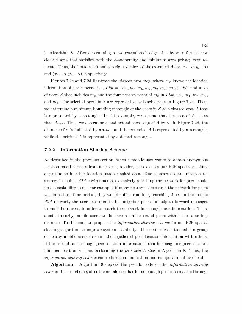
134

in Algorithm 8. After determining α, we extend each edge of A by α to form a new

cloaked area that satisfies both the k-anonymity and minimum area privacy require-

ments. Thus, the bottom-left and top-right vertices of the extended A are (xs−α, ys−α)

and (xe + α, ye + α), respectively.

Figures 7.2c and 7.2d illustrate the cloaked area step, where m8 knows the location

information of seven peers, i.e., List = {m4,m5,m6,m7,m9,m10,m15}. We find a set

of users S that includes m8 and the four nearest peers of m8 in List, i.e., m4, m5, m7,

and m9. The selected peers in S are represented by black circles in Figure 7.2c. Then,

we determine a minimum bounding rectangle of the users in S as a cloaked area A that

is represented by a rectangle. In this example, we assume that the area of A is less

than Amin. Thus, we determine α and extend each edge of A by α. In Figure 7.2d, the

distance of α is indicated by arrows, and the extended A is represented by a rectangle,

while the original A is represented by a dotted rectangle.

7.2.2 Information Sharing Scheme

As described in the previous section, when a mobile user wants to obtain anonymous

location-based services from a service provider, she executes our P2P spatial cloaking

algorithm to blur her location into a cloaked area. Due to scarce communication re-

sources in mobile P2P environments, excessively searching the network for peers could

pose a scalability issue. For example, if many nearby users search the network for peers

within a short time period, they would suffer from long searching time. In the mobile

P2P network, the user has to enlist her neighbor peers for help to forward messages

to multi-hop peers, in order to search the network for enough peer information. Thus,

a set of nearby mobile users would have a similar set of peers within the same hop

distance. To this end, we propose the information sharing scheme for our P2P spatial

cloaking algorithm to improve system scalability. The main idea is to enable a group

of nearby mobile users to share their gathered peer location information with others.

If the user obtains enough peer location information from her neighbor peer, she can

blur her location without performing the peer search step in Algorithm 8. Thus, the

information sharing scheme can reduce communication and computational overhead.

Algorithm. Algorithm 9 depicts the pseudo code of the information sharing

scheme. In this scheme, after the mobile user has found enough peer information through

135

Algorithm 9 Information Sharing Scheme

1: function InformationSharingScheme(User U , Tolerance tols)2: //Step 1: Peer Search Step3: List stores the received peer location information of the last peer search4: if the timestamp of the last peer search < tnow − tols then5: Request the neighbor peers to turn in their List size and the timestamp of their

last peer search tsearch

6: if some neighbor peer has List with a size of at least U.K and the timestamp ofher last peer search ≥ tnow − tols then

7: Select the neighbor peer P with the latest peer search timestamp8: Request P to turn in the cached location information of the k-nearest peers to

U9: List← the received peer location information

10: else11: return P2PSpatialCloaking(User U) (i.e., Algorithm 8)12: end if13: end if14: //Step 2: Cloaked Area Step15: Adjust the peer location information in List16: A← a minimum bounding rectangle includes U and the adjusted location region of

the K − 1 nearest P of U in List17: Execute Lines 13 to 16 in Algorithm 8 to ensure that A satisfies the minimum area

privacy requirement18: return A

the peer search step in Algorithm 8, she maintains the received peer information in List

and records the timestamp, tsearch, when the last peer search step started. Since this

scheme only provides the cached peer location information for the user, the information

could be cached a long time ago. The older the cached information, the lower the quality

of a cloaked area (i.e., the cloaked area size) will be obtained. To this end, the informa-

tion sharing scheme enables the user to control the staleness of the cached information

through a user specified parameter tols. In other words, the user only utilizes the peer’s

stored information cached not earlier than tols. The information sharing scheme can

be incorporated into our P2P spatial cloaking algorithm (i.e., Algorithm 8) with the

following modifications.

Step 1: Peer search step. The user U starts this step by checking whether she can

use her cached information and/or her neighbor peers’ cached information to blur her

136

location. U first checks the freshness of her cached peer information. If the timestamp of

the last peer search is larger than or equal to tnow− tols, where tnow is the current time,

U can reuse her cached peer information. Otherwise, U requests her neighbor peers to

reply with the size of their List along with tsearch (Line 5 in Algorithm 9). If more than

one neighbor peer caches enough peer location information and tsearch ≥ tnow − tols, U

selects the peer P caching the freshest information, i.e., the largest tsearch (Line 7 in

Algorithm 9). Then, U requests P to turn in the K − 1 nearest peer information to

U . However, if no neighbor peer caches enough peer location information or the cached

information is too stale, U simply executes the original peer search step in Algorithm 8

(Line 11 in Algorithm 9). After U receives enough peer information, U stores the peer

information in List.

Step 2: Cloaked area step. Due to user mobility, i.e., mobile users are continu-

ously moving, the only modification to this step is to capture the location uncertainty

of the cached peer information. The basic idea is that given a peer’s location cached

at time t, we use a conservative approach to determine a location region that includes

all possible locations of the peer at current time tnow. Since the current location of the

peer could be at any point within a circular area centered at the peer’s cached location

with a radius of (tnow−t)×vmax, where vmax is the maximum possible speed of the peer

and t is the time when the peer’s location information was cached, such a circular area

constitutes the peer’s adjusted location region. For a peer P with an adjusted location

region, we consider the maximum distance between U and P ’s adjusted location region,

i.e., dmax(U,P ) = d(U,P ) + (tnow − t) × vmax, as their distance. In reality, vmax can

be set to the maximum legal speed in the system area. Then, we form a k-anonymous

cloaked area A as a minimum bounding rectangle of U and the adjusted location region

of the K − 1 peers (Line 16 in Algorithm 9). If A does not satisfy the minimum area

privacy requirement, we extend A as in the original cloaked area step in Algorithm 8

(Line 17 in Algorithm 9).

7.2.3 Peer-to-Peer Spatial Cloaking in a Partitioned Network

Since we consider a highly ad hoc mobile environment, where no fixed communication

infrastructure or centralized/distributed servers are available, mobile users can only

communicate with each other via multi-hop peer-to-peer routing. Due to user mobility,

137

mobile users may be partitioned into disjoint networks. When a network partition takes

place, a mobile user can only communicate with other peers residing in her network

partition. If a user’s required anonymity level is larger than the number of users re-

siding in her network partition, the user cannot find enough peer location information

to blur her location information; and thus, the user suffers from a network partition

problem. In this section, we first discuss how to detect a network partition problem and

two straightforward approaches to alleviate it, and then propose the historical location

scheme to better alleviate the network partition problem.

We now discuss how to detect a network partition problem in the peer search step in

Algorithm 8. Let Listh be the set of peer location information that is found by the peer

search step with a hop distance h. It is expected to find more peers as h increases, i.e.,

|Listh| > |Listh−1|. Thus, we know that a network partition takes place when |Listh| =|Listh−1|. It is important to note that we only need to record the size of Listh−1 without

maintaining the peer location information. There are two straightforward approaches

that a user can use to overcome the network partition problem. (1) After the user

suffers from the network partition problem, she periodically performs the peer search

step until she can find enough peer location information. (2) After the user cannot find

an adequate number of peers in her network partition, she simply reduces her required

k-anonymity level to the number of users residing in her network partition. However,

these two straightforward approaches have drawbacks. The first approach would incur

very long searching time while the second one requires the user to degrade her privacy

protection. To this end, we propose the historical location scheme that enables the

users to utilize their or other peers’ cached information to better alleviate the network

partition problem.

Algorithm. Algorithm 10 depicts the pseudo code of the historical location scheme,

and Figure 7.3 gives an example to illustrate this scheme. Similar to the information

sharing scheme, the user can control the staleness of the historical peer location infor-

mation through a tolerance parameter tolh. Thus, this scheme only uses the historical

peer location information that was cached not earlier than tnow − tolh. When U suf-

fers from the network partition problem in the peer search step in Algorithm 8, i.e.,

|Listh| = |Listh−1| and Listh−1 < K, U sets hlast = h − 1 and executes the historical

location scheme. In general, the historical location scheme can be incorporated into our

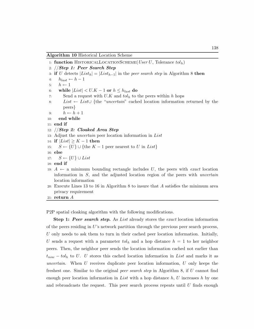
138

Algorithm 10 Historical Location Scheme

1: function HistoricalLocationScheme(User U , Tolerance tolh)2: //Step 1: Peer Search Step3: if U detects |Listh| = |Listh−1| in the peer search step in Algorithm 8 then4: hlast ← h− 15: h← 16: while |List| < U.K − 1 or h ≤ hlast do7: Send a request with U.K and tolh to the peers within h hops8: List ← List∪ {the “uncertain” cached location information returned by the

peers}9: h← h + 1

10: end while11: end if12: //Step 2: Cloaked Area Step13: Adjust the uncertain peer location information in List14: if |List| ≥ K − 1 then15: S ← {U} ∪ {the K − 1 peer nearest to U in List}16: else17: S ← {U} ∪ List18: end if19: A ← a minimum bounding rectangle includes U , the peers with exact location

information in S, and the adjusted location region of the peers with uncertainlocation information

20: Execute Lines 13 to 16 in Algorithm 8 to insure that A satisfies the minimum areaprivacy requirement

21: return A

P2P spatial cloaking algorithm with the following modifications.

Step 1: Peer search step. As List already stores the exact location information

of the peers residing in U ’s network partition through the previous peer search process,

U only needs to ask them to turn in their cached peer location information. Initially,

U sends a request with a parameter tolh and a hop distance h = 1 to her neighbor

peers. Then, the neighbor peer sends the location information cached not earlier than

tnow − tolh to U . U stores this cached location information in List and marks it as

uncertain. When U receives duplicate peer location information, U only keeps the

freshest one. Similar to the original peer search step in Algorithm 8, if U cannot find

enough peer location information in List with a hop distance h, U increases h by one

and rebroadcasts the request. This peer search process repeats until U finds enough

139

��

��

��

��

��

��

��

��

��

��

(a) Partitioned Network

��

��

��

��

��

��

(b) Historical Location Scheme

Figure 7.3: Example of peer-to-peer spatial cloaking in a partitioned network.

peer location information or h = hlast (Lines 6 to 10 in Algorithm 10). After U finishes

the peer search process, she proceeds to the next step regardless of whether List stores

enough peer location information.

Step 2: Cloaked area step. The user U starts this step by adjusting the uncertain

peer location information in List as in the information sharing scheme. If |List| ≥U.K−1, U adds the K−1 nearest peers in List and herself to S (Line 15 in Algorithm 10).

For a peer P with uncertain location information, the distance between U and P is the

maximum distance between U and the adjusted location region of P , i.e., dmax(U,P ) =

d(U,P )+(tnow− t)×vmax. However, if |List| ≤ U.K, we use the second straightforward

approach to temporally reduce U.K to |List|+ 1 (Line 17 in Algorithm 10); and thus,

U simply adds all peers in List and herself to S. Then, U forms a cloaked area A that

includes the peers with the exact location information and the adjusted location region

of the peers with the uncertain location information in S (Line 19 in Algorithm 10).

If A does not satisfy the minimum area privacy requirement, we extend A as in the

original cloaked area step in Algorithm 8 (Line 20 in Algorithm 10).

Example. Figure 7.3 depicts an example of a partitioned network where the mobile

users are partitioned into two disjoint networks. One network partition includes five

mobile users m1 to m5, while the other partition includes five mobile users m6 to m10

(Figure 7.3a). Each user is labeled with a pair of values, where the first value is her

identity and the second value is her required anonymity level. In this example, m4

(represented by a black circle) executes the P2P spatial cloaking algorithm to blur

her location into a cloaked area. Since the number of users residing in m4’s network

140

partition is less than her required anonymity level, i.e., m4.K = 6, m4 suffers from

the network partition problem. After m4 performs the peer search process with a hop

distance of h = 3, she detects the network partition problem because |List2| = |List3|(i.e., hlast = 2). We assume that m5 caches the location information of m6. Thus,

m4 can find enough peer location information after she enlists the peers within two

hop distance for help to turn in their cached location information. List stores the

location information of five peers, i.e., List = {m1,m2,m3,m5,m6}, where the peer

with uncertain location information is underlined. Then, m4 adjusts m6’s location

information, and the adjusted location region of m6 is represented by a dotted circle,

as depicted in Figure 7.3b. The cloaked area A of m4 that is represented by a rectangle

includes m4, the peers with exact location information in List, i.e., m1, m2, m3, and

m5, and the adjusted location region of m6 (i.e., the dotted circle). We assume that A

satisfies m4’s minimum area privacy requirement, so A is returned to m4 as her cloaked

area.

7.2.4 Cloaked Area Adjustment Scheme

As discussed in Section 7.2.1, our P2P spatial cloaking selects the nearest peers of a

mobile user to form her cloaked area A. This peer selection process may pose a privacy

breach that the query issuer tends to be the closest to the center of A, i.e., the “center-

of-cloaked-area” privacy attack [39, 44, 108]. Such a privacy breach may give more

information to an adversary to infer the query issuer’s actual location. To prevent

this privacy breach, we should adjust A such that the probability of the query issuer

being the closest to the center of A is 1/K. To this end, we propose the cloaked area

adjustment scheme that prevents the “center-of-cloaked-area” privacy attack if the user

knows the exact location information of the peers residing in A. In case that the user

only knows the historical location information of some peers residing in A, the cloaked

area adjustment scheme can still alleviate the “center-of-cloaked-area” privacy attack.

We will evaluate the resistance of our cloaked area adjustment scheme to this privacy

attack through extensive experiments in Section 7.4.1.

Algorithm. Algorithm 11 gives the pseudo code of the cloaked area adjustment

scheme. This algorithm is called by Algorithm 8 after executing Line 12; thus, we

141

Algorithm 11 Cloaked Area Adjustment Scheme

1: function CloakedAreaAdjustment(User U , UserSet S, Area A)2: C ′

A ← CA; A′ = {(x′s, y

′s), (x

′e, y

′e)} ← A = {(xs, ys), (xe, ye)}

3: PC ← the nearest user in S to CA

4: P ← a randomly selected user in S5: if P 6= PC then6: //Step 1: Center Adjustment Step7: PN ← the nearest user in S to P8: M ← the intersection point between line PCA and the circle centered at P with

a radius of d(P, PN )/29: R← a random value within a range of (d(M,CA), d(P,CA)]

10: C ′A ←

([d(P,CA)−R]×CA.x+R×P.x

d(P,CA) , [d(P,CA)−R]×CA.y+R×P.y

d(P,CA)

)

11: //Step 2: Area Adjustment Step12: ∆x ← |C ′

A.x− CA.x|13: ∆y ← |C ′

A.y −CA.y|14: if C ′

A.x < CA.x then x′s ← xs − 2∆x; else x′

e ← xe + 2∆x

15: if C ′A.y < CA.y then y′s ← ys − 2∆y; else y′e ← ye + 2∆y

16: end if17: return A′

add the statement “A ← CloakedAreaAdjustment(U, S,A)” after Line 12 in Al-

gorithm 8. The inputs to the algorithm include a user U , a set of users S selected by

the cloaked area step in Algorithm 8, and a minimum bounding box of the users in S,

A. A is represented by its bottom-left vertex (xs, ys) and top-right vertex (xe, ye), and

the center of A is CA = ((xs + xe)/2, (ys + ye)/2). The output of this algorithm is

an adjusted cloaked area A′ that is represented by its bottom-left vertex (x′s, y

′s) and

top-right vertex (x′e, y

′e), and C ′

A is the center of A′. Initially, we set A′ = A (Line 2

in Algorithm 11). For the peer with historical location information in S, we consider

the center of her adjusted location region as her location. We start this algorithm by

randomly selecting a user P in S and finding the nearest user PC in S to the center of

A, CA. If P = PC , we simply return the original A to Algorithm 8; otherwise, we have

to adjust A by the following two main steps.

Step 1: Center adjustment step. Figure 7.4a illustrates this step where the

gray and black squares represent the center of the input A (CA) and the center of the

adjusted A′ (C ′A), respectively. The user U starts this step by finding the nearest user

PN in S to P . Then, U computes the intersection point M between line PCA and the

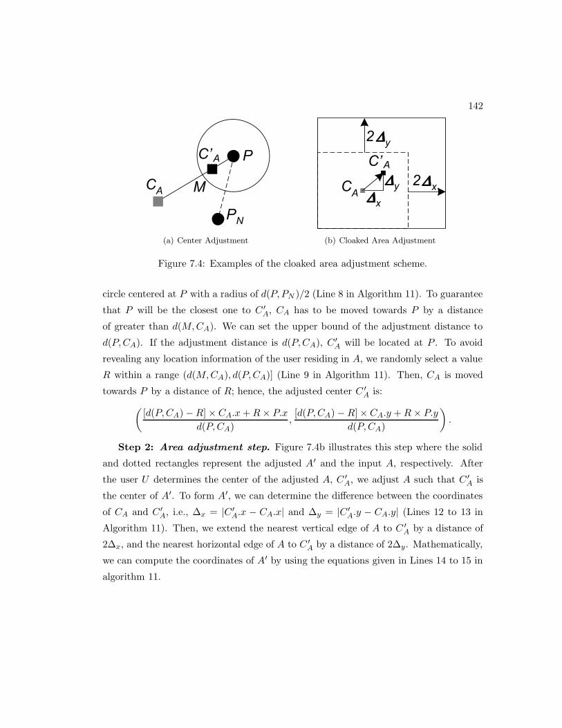
142

��

�

��

��

(a) Center Adjustment

�∆∆∆∆��∆∆∆∆��

�∆∆∆∆�

�∆∆∆∆�

��

��

��

��

(b) Cloaked Area Adjustment

Figure 7.4: Examples of the cloaked area adjustment scheme.

circle centered at P with a radius of d(P, PN )/2 (Line 8 in Algorithm 11). To guarantee

that P will be the closest one to C ′A, CA has to be moved towards P by a distance

of greater than d(M,CA). We can set the upper bound of the adjustment distance to

d(P,CA). If the adjustment distance is d(P,CA), C ′A will be located at P . To avoid

revealing any location information of the user residing in A, we randomly select a value

R within a range (d(M,CA), d(P,CA)] (Line 9 in Algorithm 11). Then, CA is moved

towards P by a distance of R; hence, the adjusted center C ′A is:

([d(P,CA)−R]× CA.x + R× P.x

d(P,CA),[d(P,CA)−R]× CA.y + R× P.y

d(P,CA)

).

Step 2: Area adjustment step. Figure 7.4b illustrates this step where the solid

and dotted rectangles represent the adjusted A′ and the input A, respectively. After

the user U determines the center of the adjusted A, C ′A, we adjust A such that C ′

A is

the center of A′. To form A′, we can determine the difference between the coordinates

of CA and C ′A, i.e., ∆x = |C ′

A.x − CA.x| and ∆y = |C ′A.y − CA.y| (Lines 12 to 13 in

Algorithm 11). Then, we extend the nearest vertical edge of A to C ′A by a distance of

2∆x, and the nearest horizontal edge of A to C ′A by a distance of 2∆y. Mathematically,

we can compute the coordinates of A′ by using the equations given in Lines 14 to 15 in

algorithm 11.

143

��

��

��

��

��

��

��

��

�

�

��

��

��

��

��

��

��

��

��

��

��

��

��

��

��

��

��

��

��

��

��

��

(a) Server Side

��

��

��

��

��

��

��

��

�

�

��

��

��

��

��

��

��

��

��

��

��

��

��

��

��

��

��

��

��

��

��

��

(b) Client Side

Figure 7.5: Privacy-aware nearest-neighbor query processing.

7.3 Anonymous Location-based Services

To enable location-based database servers to support privacy-aware location-based

queries with cloaked areas rather than with exact location points, the database server

needs to be equipped with a privacy-aware query processor [17, 80, 44, 12]. In this pa-

per, we adopt the work [80] as our privacy-aware query processor because it minimizes

the communication overhead of sending a minimal answer set from the database server

to the user while guaranteeing the user can get the exact answer. When a user wants

to issue a privacy-aware location-based queries, she executes our P2P spatial cloaking

algorithm to blur her location into a cloaked area. Then, the user sends the query along

with the cloaked area to the location-based database server. After the privacy-aware

query processor computes a minimal answer set that includes the exact answer to the

user, the database server sends the answer set to the user. Finally, the user computes

the exact answer from the answer set. The smaller the cloaked area, the smaller the

answer set will be returned to the user. However, the user may need to relax her pri-

vacy requirements to achieve a smaller cloaked area. Thus, a trade-off between the user

privacy protection and the quality of services can be achieved.

Figure 7.5 illustrates the privacy-aware nearest-neighbor query processing. Fig-

ure 7.5a depicts the data objects, e.g., gas stations, stored at the server side. There

are 32 data objects T1 to T32 represented by black circles, the shaded area represents

144

Table 7.1: Summary of the features of our algorithms.

P2P P2P-IS P2P-IS-CA P2P-IS-CA-HL

Peer-to-Peer Spatial Cloaking (P2P)√ √ √ √

Information Sharing Scheme (IS) × √ √ √

Cloaked Area Adjustment Scheme (CA) × × √ √

Historical Location Scheme (HL) × × × √

the cloaked area of the mobile user who issued the query. For clarification, the actual

mobile user location is plotted in Figure 7.5 as a black square inside the cloaked area A,

i.e., the shaded area. However, such information is neither stored at the server side nor

revealed to the server. The privacy-aware query processor determines a minimal answer

set that includes the nearest object to every point within A. It has been proved that

the minimal answer set includes all objects within A and the nearest object to every

point of each edge of A [80]. In this example, the server returns the answer set that

includes six objects, i.e., T8, T12, T13, T16, T17, and T22, to the user. Then, the user

computes the exact answer, i.e., T13, from the answer set. The algorithmic detail of the

privacy-aware query processor is beyond the scope of this paper. Interested readers are

referred to [80] for more details.


In this section, we evaluate the performance of our P2P spatial cloaking algorithm (de-

noted as P2P) with the three key features, information sharing scheme (denoted as

IS), historical location scheme (denoted as HL), and cloaked area adjustment scheme

(denoted as CA) through simulated experiments. Our P2P spatial cloaking algorithm

(P2P) corresponds to the on-demand approach of the state-of-the-art P2P spatial cloak-

ing algorithm [19]. We do not consider the proactive approach because its communica-

tion overhead is much higher than the on-demand approach. Table 7.1 summaries the

features of our algorithms.

We evaluate our algorithms with respect to five important performance measures.

(1) Number of messages. This measure gives the average number of messages incurred

145

by our algorithms per each query. It indicates the network bandwidth consumption and

the power consumption on user devices. (2) Cloaked area size. This measure gives the

average size of cloaked areas generated by our algorithms. The smaller the cloaked area,

the more accurate the location is reported to the location-based database server; the

thus, this measure can indicate the location utility of our algorithms. (3) Answer set size.

This measure indicates the average number of objects included in answer sets returned

by the location-based database server. It also indicates the communication overhead of

sending the answer set from the database server to the user. (4) Anonymization success

rate. This is a ratio of the number of times that the anonymization algorithm can find

enough peer location information to satisfy the user’s k-anonymity privacy requirement

to the total number of queries. (5) Privacy attack probability. This measure gives the

resilience of our algorithms to the “center-of-cloaked-area” privacy attack by measuring

the probability of the nearest user to the center of a cloaked area (Uc) being the actual

query issuer, i.e., P(Uc is the query issuer).

We use a networked generator to generate moving objects on the road map of Hen-

nepin County, Minnesota, USA. The road map consists of 57,020 edges and 42,135

vertices. Unless mentioned otherwise, all our experiments consider 100,000 mobile users

in which 10% of them are randomly selected to issue nearest-neighbor queries (e.g.,

“where is my nearest gas station”) at each time instance. The mobile users are moving

at speeds between 50 and 70 miles per hour. Their required k-anonymity levels are

uniformly selected from a range [50, 100], while their required minimum areas are set

to zero. There are 20,000 data objects that are uniformly distributed within the under-

lying road map. The default uncertainty tolerance for the information sharing scheme

(tols) and historical location scheme (tolh) is set to zero and 50 seconds, respectively.

We consider a heterogeneous network environment where the transmission range of each

user is uniformly selected within a range [100, 200] meters. Table 9.1 summarizes the

parameter settings.

7.4.1 Anonymization Strength

Figure 7.6 depicts the resilience of our algorithms to the “center-of-cloaked-area” privacy

attack with respect to varying (a) the k-anonymity level from 100 to 300, (b) the number

of users from 100,000 to 500,000, (c) the transmission range from [100, 100] to [100, 300]

146

Table 7.2: Parameter settings.Parameters Default values Ranges

Number of users 200K 100K to 500KNumber of querying users 20K 10K to 50KNumber of data objects 20K 10K to 50K

Transmission range [100, 200] meters [100, 100] to [100, 300] metersk-anonymity [50, 100] [50, 100] to [50, 300]

Minimum area Amin 0 1 to 5 km2

tols 0 0 to 50 secondstolh 50 seconds -

Movement speed [50, 70] miles per hour -

meters, and (d) the uncertainty tolerance for the information sharing scheme, i.e., tols,

from 0 to 50 seconds. The default k-anonymity level for (b)-(d) is 100. The results

of P2P-IS-CA-HL, P2P-IS-CA, P2P-IS, and P2P are represented by black, gray, light

gray, and white bars, respectively. The pattern bars represent the value of 1/K which

indicates the ideal probability of the actual query issuer being the nearest user to the

center of the cloaked area Uc, i.e., P(Uc is the query issuer). Although P2P is more

vulnerable to the “center-of-cloaked-area” attack than P2P-IS (Figures 7.6a-7.6d), the

probability of both P2P and P2P-IS are way above the ideal probability. The results

show that our cloaked area adjustment scheme (CA) gives the probability of Uc being the

actual query issuer is equal to or very close to 1/K. Thus, our cloaked area adjustment

scheme can effectively prevent the “center-of-cloaked-area” privacy attack.

7.4.2 Scalability

In this section, we evaluate the scalability of our algorithms with respect to large num-

bers of querying users, large numbers of users, and large numbers of data objects.

Figure 7.7 depicts the performance of our algorithms with respect to varying the

number of querying users from 10,000 to 50,000 users, i.e., from 5% to 25% of 200,000

users. The performance of P2P is not affected by the number of querying users because

there is no information sharing among users in P2P. The results show that our infor-

mation sharing scheme (i.e., P2P-IS, P2P-IS-CA, and P2P-IS-CA-HL) effectively reduces

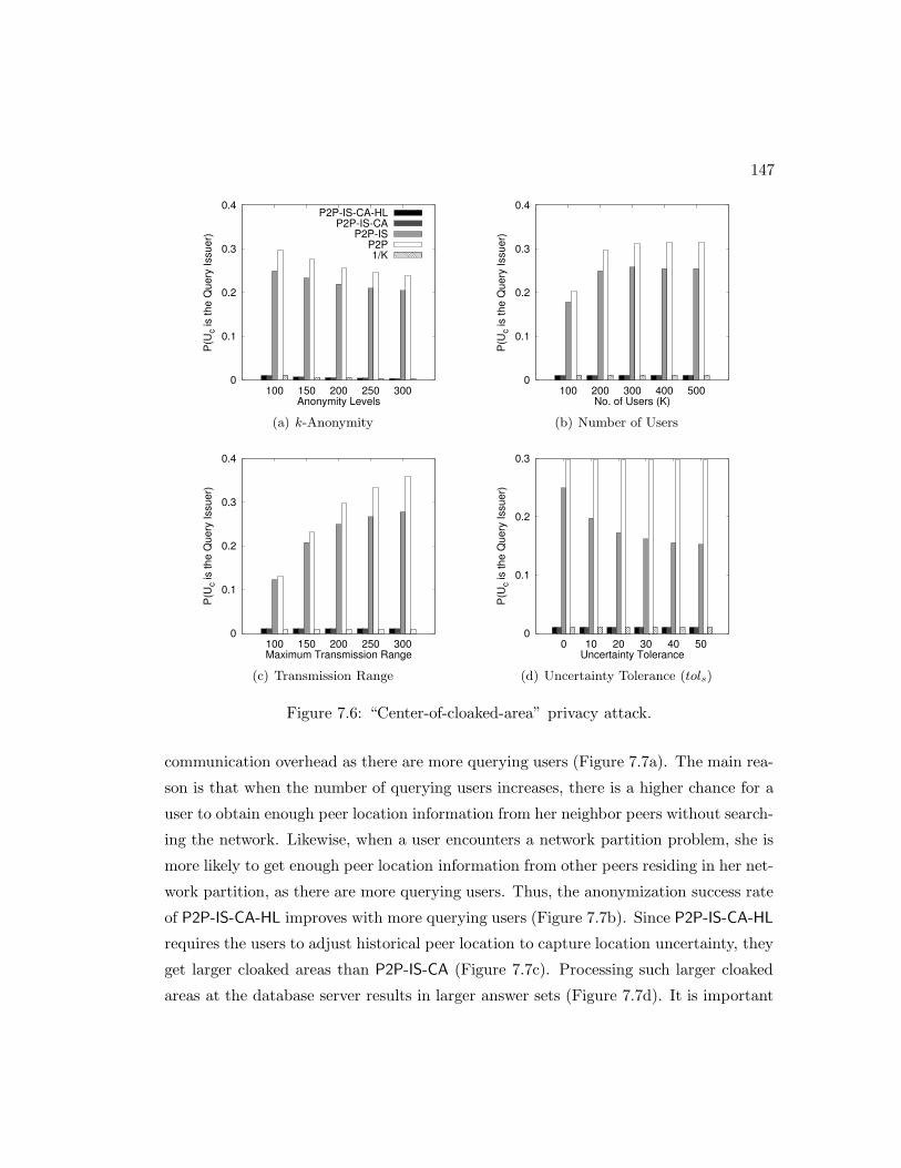
147

0

0.1

0.2

0.3

0.4

100 150 200 250 300

P(U

c is

the

Que

ry Is

suer

)

Anonymity Levels

P2P-IS-CA-HLP2P-IS-CA

P2P-ISP2P1/K

(a) k-Anonymity

0

0.1

0.2

0.3

0.4

100 200 300 400 500

P(U

c is

the

Que

ry Is

suer

)

No. of Users (K)

(b) Number of Users

0

0.1

0.2

0.3

0.4

100 150 200 250 300

P(U

c is

the

Que

ry Is

suer

)

Maximum Transmission Range

(c) Transmission Range

0

0.1

0.2

0.3

0 10 20 30 40 50

P(U

c is

the

Que

ry Is

suer

)

Uncertainty Tolerance

(d) Uncertainty Tolerance (tols)

Figure 7.6: “Center-of-cloaked-area” privacy attack.

communication overhead as there are more querying users (Figure 7.7a). The main rea-

son is that when the number of querying users increases, there is a higher chance for a

user to obtain enough peer location information from her neighbor peers without search-

ing the network. Likewise, when a user encounters a network partition problem, she is

more likely to get enough peer location information from other peers residing in her net-

work partition, as there are more querying users. Thus, the anonymization success rate

of P2P-IS-CA-HL improves with more querying users (Figure 7.7b). Since P2P-IS-CA-HL

requires the users to adjust historical peer location to capture location uncertainty, they

get larger cloaked areas than P2P-IS-CA (Figure 7.7c). Processing such larger cloaked

areas at the database server results in larger answer sets (Figure 7.7d). It is important

148

0.2

0.3

0.4

0.5

0.6

0.7

10 20 30 40 50

Ave

rage

No.

of M

essa

ges

(K)

No. of Querying Users (K)


P2P-ISP2P

(a) Communication Overhead

0.93

0.94

0.95

0.96

0.97

10 20 30 40 50

Ano

nym

izat

ion

Suc

cess

Rat

e


(b) Anonymization Success Rate

0.5

0.6

0.7

0.8

0.9

1

1.1

1.2

1.3

1.4

10 20 30 40 50

Ave

rage

Clo

aked

Are

a S

ize

(km

2 )


(c) Cloaked Area Size

14

16

18

20

22

24

26

10 20 30 40 50

Ave

rage

Ans

wer

Set

Siz

e


(d) Answer Set Size

Figure 7.7: Number of querying users.

to note that although our algorithms with the cloaked area adjustment scheme, i.e.,

P2P-IS-CA and P2P-IS-CA-HL, result in larger cloaked areas and answer sets than P2P

and P2P-IS, P2P-IS-CA and P2P-IS-CA-HL are free from the “center-of-cloaked-area”

privacy attack.

Figure 7.8 depicts the scalability of our algorithms with respect to increasing the

number of users from 100,000 to 500,000. The results show that the performance of all

algorithms gets better when there are more users. In a denser network, the user can

find enough peer information to blur her location with a smaller hop distance, i.e., a

smaller searching area; and hence, the communication overhead reduces (Figure 7.8a).

When the number of users increases, there are more users in a network partition. Thus,

149

0.1

0.2

0.3

0.4

0.5

0.6

0.7

0.8

0.9

1

100 200 300 400 500

Ave

rage

No.

of M

essa

ges

(K)

No. of Users (K)


P2P-ISP2P


0.7

0.75

0.8

0.85

0.9

0.95

1

100 150 200 250 300

Ano

nym

izat

ion

Suc

cess

Rat

e

No. of Users (K)


0

0.5

1

1.5

2

2.5

100 200 300 400 500

Ave

rage

Clo

aked

Are

a S

ize

(km

2 )

No. of Users (K)


5

10

15

20

25

30

35

40

45

50

100 200 300 400 500

Ave

rage

Ans

wer

Set

Siz

e

No. of Users (K)

(d) Answer Set Size

Figure 7.8: Number of users.

it is more likely that the user can find enough peer location information in her network

partition, i.e., the anonymization success rate improves (Figure 7.8b). Since the users

can blur their locations into smaller cloaked areas in the denser network (Figure 7.8c),

the database server returns smaller answer sets to them (Figure 7.8d).

Figure 7.9 depicts the scalability of our algorithms with respect to varying the num-

ber of data objects from 10,000 to 50,000. Since increasing the number of data objects at

the database server only affects the answer set size, the performance of the peer search

process and the spatial cloaking process of all algorithms is not affected. Figure 7.9b

gives that the answer set size of all algorithms linearly increases as there are more data

objects.

150

0.4

0.6

0.8

1

1.2

1.4

1.6

10 20 30 40 50

Ave

rage

Clo

aked

Are

a S

ize

(km

2 )

No. of Data Objects (K)


P2P-ISP2P

(a) Cloaked Area Size

5

10

15

20

25

30

35

40

45

50

55

10 20 30 40 50

Ave

rage

Ans

wer

Set

Siz

e

No. of Data Objects (K)

(b) Answer Set Size

Figure 7.9: Number of data objects.


In this section, we evaluate the performance of our algorithms with respect to the user

specified k-anonymity and minimum area Amin privacy requirements.

Figure 7.10 depicts the performance of our algorithms with the increase of the strict-

ness of the k-anonymity privacy requirement from [50, 100] and [50, 300]. It is expected

that the performance of all algorithms becomes worse as the k-anonymity privacy re-

quirement gets stricter. When k increases, the user needs to enlist more peers for help

to gather enough peer location information, so the communication overhead gets higher

(Figure 7.10a). Our algorithms with the information sharing scheme (i.e., P2P-IS, P2P-

IS-CA, and P2P-IS-CA-HL) perform better than P2P as k gets larger. Since the user

with a stricter k-anonymity privacy requirement needs to gather more peer location

information to blur her location, she is more likely to encounter the network partition

problem (Figure 7.10b). The results show that the user adopting our historical location

scheme (i.e., P2P-IS-CA-HL) records a higher anonymization success rate than other

algorithms. Figure 7.10c depicts that all algorithms generate larger cloaked areas to

satisfy stricter privacy requirements. With larger cloaked areas, it is expected that the

database server returns larger answer sets to the user (Figure 7.10d).

Figure 7.11 gives the performance of our algorithms with respect to increasing the

required minimum area Amin of cloaked areas from 1 to 5 km2. In this experiment, we

set the anonymity level to a smaller value, i.e., K = 10, so the results mainly depend

151

0

0.5

1

1.5

2

2.5

3

100 150 200 250 300

Ave

rage

No.

of M

essa

ges

(K)

Anonymity Levels


P2P-ISP2P


0.91

0.92

0.93

0.94

0.95

0.96

100 150 200 250 300

Ano

nym

izat

ion

Suc

cess

Rat

e

Anonymity Levels


0.5

1

1.5

2

2.5

3

3.5

100 150 200 250 300

Ave

rage

Clo

aked

Are

a S

ize

(km

2 )

Anonymity Levels


10

15

20

25

30

35

40

45

50

55

100 150 200 250 300

Ave

rage

Ans

wer

Set

Siz

e

Anonymity Levels

(d) Answer Set Size

Figure 7.10: k-anonymity privacy requirements.

on Amin. Varying Amin only affects the cloaked area size and the answer set size. It is

interesting to see that when Amin is stricter than the k-anonymity privacy requirement,

all algorithms give similar results in terms of cloaked area size and answer set size, as

depicted in Figures 7.11a and 7.11b, respectively. It is expected that all algorithms

generate larger cloaked areas as Amin gets stricter. When a cloaked area A gets larger,

it is more likely that A includes a larger set of data objects and each edge of A has

a larger set of nearest data objects. Thus, the answer set size increases as Amin gets

stricter.

152

0

1

2

3

4

5

6

1 2 3 4 5

Ave

rage

Clo

aked

Are

a S

ize

(km

2 )

Minimum Area (km2)


P2P-ISP2P

(a) Cloaked Area Size

20

30

40

50

60

70

80

90

100

1 2 3 4 5

Ave

rage

Ans

wer

Set

Siz

e

Minimum Area (km2)

(b) Answer Set Size

Figure 7.11: Minimum area privacy requirements.

7.4.4 Effect of Transmission Range

Figure 7.12 depicts the performance of our algorithms respect to increasing the transmis-

sion range of user mobile devices from [100, 100] to [100, 300] meters. If the transmission

range gets larger, the user can find enough peer location information within a smaller

hop distance; and thus, the communication overhead reduces (Figure 7.12a). As the

transmission range gets larger, our algorithms can find k-anonymized cloaked areas for

the users with stricter anonymity levels, so the anonymization success rate improves

(Figure 7.12b). However, the stricter the anonymity level, the lager the cloaked area

size is generated by our algorithms, so all algorithms generates larger cloaked areas as

the transmission range increases (Figure 7.12c). Since the increase of the cloaked area

size is small, the answer set size is slightly affected (Figure 7.12d).

7.4.5 Effect of Uncertainty Tolerance

Figure 7.13 gives the performance of our algorithms respect with to varying the user

uncertainty tolerance level for the information sharing scheme, i.e., tols, from 0 to 50

seconds. Since P2P does not support information sharing among users, varying tols

does not affect its performance. When the user is willing to utilize staler peer location

information, it is easier for her to obtain enough peer location information from her

neighbor peers without searching the network. Thus, the communication overhead of

153

0.2

0.4

0.6

0.8

1

1.2

1.4

1.6

100 150 200 250 300

Ave

rage

No.

of M

essa

ges

(K)



P2P-ISP2P


0.6

0.7

0.8

0.9

1

100 150 200 250 300

Ano

nym

izat

ion

Suc

cess

Rat

e



0

0.2

0.4

0.6

0.8

1

1.2

1.4

100 150 200 250 300

Ave

rage

Clo

aked

Are

a S

ize

(km

2 )



0

5

10

15

20

25

30

100 150 200 250 300

Ave

rage

Ans

wer

Set

Siz

e


(d) Answer Set Size

Figure 7.12: Transmission range.

the algorithms with the information sharing scheme (i.e., P2P-IS, P2P-IS-CA, and P2P-

IS-CA-HL) reduces, as tols gets larger (Figure 7.13a). Likewise, when the user accepts

a larger tols, there is a higher chance for her to find enough peer location information

within her network partition; and therefore, the user experiences a higher anonymization

success rate as tols increases (Figure 7.13b). With respect to cloaked area size, all

algorithms generate larger cloaked areas, as tols increases (Figure 7.13c). This is due to

the fact that we need larger adjusted location regions for staler peer location information

in order to capture its uncertainty. It is expected that the answer set size increases as

the cloaked area gets larger (Figure 7.13d).

154

0.1

0.2

0.3

0.4

0.5

0.6

0.7

0.8

0 10 20 30 40 50

Ave

rage

No.

of M

essa

ges

(K)



P2P-ISP2P


0.94

0.95

0.96

0.97

0 10 20 30 40 50

Ano

nym

izat

ion

Suc

cess

Rat

e



0.5

1

1.5

2

2.5

3

0 10 20 30 40 50

Ave

rage

Clo

aked

Are

a S

ize

(km

2 )



10

15

20

25

30

35

40

45

0 10 20 30 40 50

Ave

rage

Ans

wer

Set

Siz

e


(d) Answer Set Size

Figure 7.13: Uncertainty tolerance for the information sharing scheme (tols).

7.5 Summary

In this chapter, we present a peer-to-peer (P2P) spatial cloaking algorithm that enables

mobile users to obtain location-based services without revealing their exact location in-

formation. Our P2P spatial cloaking algorithm is designed for mobile P2P environments

in which no fixed communication infrastructure or centralized/distributed servers are

available. The main idea of our algorithm is that when a mobile user wants to obtain

location-based services, she collaborates with other peers to blur her location into a

cloaked area. Our algorithm guarantees the cloaked area satisfies the user specified k-

anonymity and minimum area Amin privacy requirements, i.e., the cloaked area includes

at least k users and has a size of at least Amin. To overcome the limitations of mobile

155

P2P environments, e.g., user mobility, limited transmission range, scarce communica-

tion resources, multi-hop communication, and network partition problem, we propose

three key features for our algorithm. (1) The information sharing scheme enables mo-

bile users to share their gathered peer location information with nearby peers in order

to reduce communication overhead. (2) The historical location scheme allows users to

utilize historical peer location information cached by other peers to alleviate the network

partition problem. (3) The cloaked area adjustment scheme aims to adjust a cloaked

area to guarantee that the adjusted cloaked area is free from a “center-of-cloaked area”

privacy attack. We evaluate our P2P spatial cloaking algorithm with the three key fea-

tures through extensive experiments. The experimental results show that our algorithm

is scalable and efficient while guaranteeing the user’s location privacy protection.

Chapter 8

The TinyCasper System

This chapter presents the architecture and system model of the TinyCasper system; a

privacy-preserving location monitoring system in wireless sensor networks. Monitoring

personal locations with a potentially untrusted location monitoring system poses privacy

threats to the monitored individuals, because an adversary could abuse the location

information gathered by the system to infer personal sensitive information [22, 23, 24,

25]. For the location monitoring system using identity sensors, the sensor nodes report

the exact location information of the monitored persons to the server; thus using identity

sensors immediately poses a major privacy breach. To tackle such a privacy breach, the

concept of aggregate location information, that is, a collection of location data relating to

a group or category of persons from which individual identities have been removed [25,

109], has been suggested as an effective approach to preserve location privacy [23, 25,

109]. Although the counting sensors by nature provide aggregate location information,

they would also pose privacy breaches.

Figure 8.1 gives an example of a privacy breach in a location monitoring system with

counting sensors. There are 11 counting sensor nodes installed in nine rooms R1 to R9,

and two hallways C1 and C2 (Figure 8.1a). The non-zero number of persons detected

by each sensor node is depicted as a number in parentheses. Figures 8.1b and 8.1c give

the numbers reported by the same set of sensor nodes at two consecutive time instances

ti+1 and ti+2, respectively. If R3 is Alice’s office room, an adversary knows that Alice

is in room R3 at time ti. Then the adversary knows that Alice left R3 at time ti+1 and

went to C2 by knowing the number of persons detected by the sensor nodes in R3 and

156

157

��

��

��

��

��

��

��

��

��

��

��

�

�

��

��

(a) At time ti

��

��

��

��

��

��

��

��

��

��

�

�

��

��

(b) At time ti+1

��

��

��

��

��

��

��

��

��

��

�

�

��

��

(c) At time ti+2

Figure 8.1: A location monitoring system using counting sensors.

C2. Likewise, the adversary can infer that Alice left C2 at time ti+2 and went to R7.

Such knowledge leakage may lead to several privacy threats. For example, knowing that

a person has visited certain clinical rooms may lead to knowing the her health records.

Also, knowing that a person has visited a certain bar or restaurant in a mall building

may reveal confidential personal information.

This paper proposes a privacy-preserving location monitoring system for wireless

sensor networks to provide monitoring services. Our system relies on the well established

k-anonymity privacy concept, which requires each person is indistinguishable among k

persons. In our system, each sensor node blurs its sensing area into a cloaked area, in

which at least k persons are residing. Each sensor node reports only aggregate location

information, which is in a form of a cloaked area, A, along with the number of persons,

N , located in A, where N ≥ k, to the server. It is important to note that the value

of k achieves a trade-off between the strictness of privacy protection and the quality

of monitoring services. A smaller k indicates less privacy protection, because a smaller

cloaked area will be reported from the sensor node; hence better monitoring services.

However, a larger k results in a larger cloaked area, which will reduce the quality of

monitoring services, but it provides better privacy protection. Our system can avoid

158

the privacy leakage in the example given in Figure 8.1 by providing low quality location

monitoring services for small areas that the adversary could use to track users, while

providing high quality services for larger areas. The definition of a small area is relative

to the required anonymity level, because our system provides better quality services for

the same area if we relax the required anonymity level. Thus the adversary cannot infer

the number of persons currently residing in a small area from our system output with

any fidelity; therefore the adversary cannot know that Alice is in room R3.

To preserve personal location privacy, we propose two in-network aggregate location

anonymization algorithms, namely, resource- and quality-aware algorithms. Both algo-

rithms require the sensor nodes to collaborate with each other to blur their sensing areas

into cloaked areas, such that each cloaked area contains at least k persons to constitute

a k-anonymous cloaked area. The resource-aware algorithm aims to minimize commu-

nication and computational cost, while the quality-aware algorithm aims to minimize

the size of the cloaked areas, in order to maximize the accuracy of the aggregate loca-

tions reported to the server. In the resource-aware algorithm, each sensor node finds an

adequate number of persons, and then it uses a greedy approach to find a cloaked area.

On the other hand, the quality-aware algorithm starts from a cloaked area A, which is

computed by the resource-aware algorithm. Then A will be iteratively refined based on

extra communication among the sensor nodes until its area reaches the minimal possible

size. For both algorithms, the sensor node reports its cloaked area with the number of

monitored persons in the area as an aggregate location to the server.

Although our system only knows the aggregate location information about the mon-

itored persons, it can still provide monitoring services through answering aggregate

queries, for example, “What is the number of persons in a certain area?” To support

these monitoring services, we propose a spatial histogram that analyzes the gathered

aggregate locations to estimate the distribution of the monitored persons in the system.

The estimated distribution is used to answer aggregate queries.

We evaluate our system through simulated experiments in Section 9.4. The re-

sults show that the communication and computational cost of the resource-aware al-

gorithm is lower than the quality-aware algorithm, while the quality-aware algorithm

provides more accurate monitoring services (the average accuracy is about 90%) than

the resource-aware algorithm (the average accuracy is about 75%). Both algorithms only

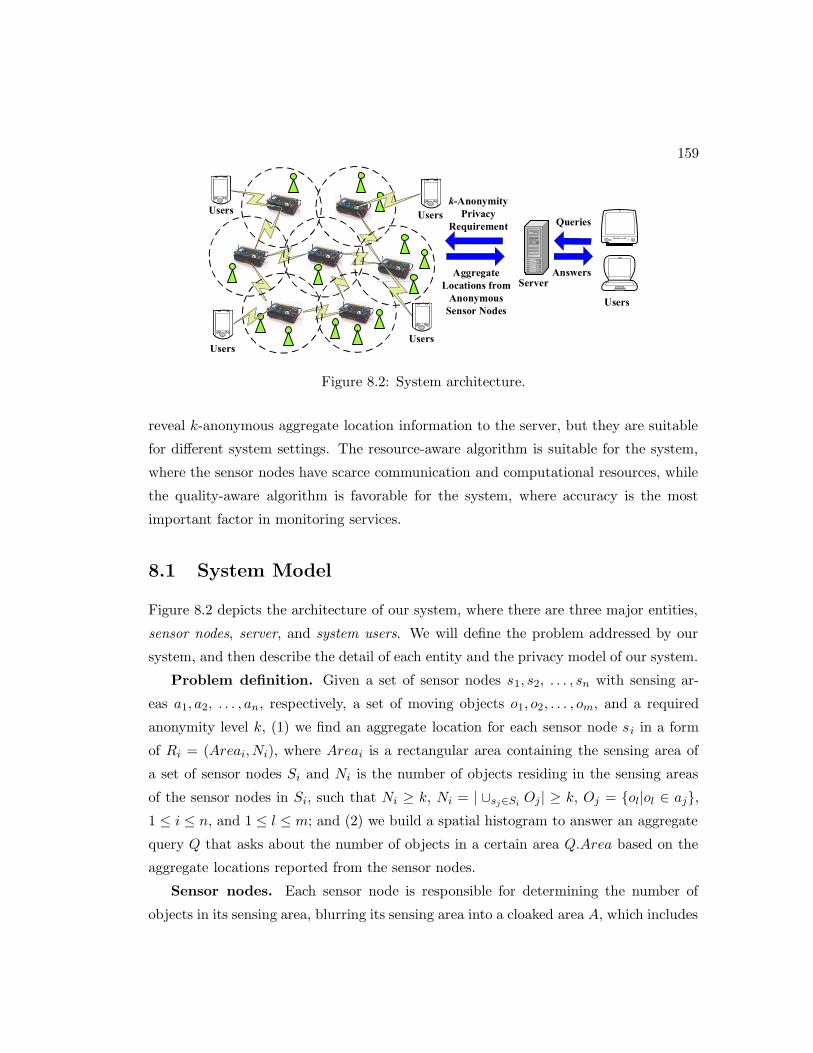
159

��

��

��

��

��

��

��

��

��

��

��

��

��

��

Figure 8.2: System architecture.

reveal k-anonymous aggregate location information to the server, but they are suitable

for different system settings. The resource-aware algorithm is suitable for the system,

where the sensor nodes have scarce communication and computational resources, while

the quality-aware algorithm is favorable for the system, where accuracy is the most

important factor in monitoring services.

8.1 System Model

Figure 8.2 depicts the architecture of our system, where there are three major entities,

sensor nodes, server, and system users. We will define the problem addressed by our

system, and then describe the detail of each entity and the privacy model of our system.

Problem definition. Given a set of sensor nodes s1, s2, . . . , sn with sensing ar-

eas a1, a2, . . . , an, respectively, a set of moving objects o1, o2, . . . , om, and a required

anonymity level k, (1) we find an aggregate location for each sensor node si in a form

of Ri = (Areai, Ni), where Areai is a rectangular area containing the sensing area of

a set of sensor nodes Si and Ni is the number of objects residing in the sensing areas

of the sensor nodes in Si, such that Ni ≥ k, Ni = | ∪sj∈SiOj | ≥ k, Oj = {ol|ol ∈ aj},

1 ≤ i ≤ n, and 1 ≤ l ≤ m; and (2) we build a spatial histogram to answer an aggregate

query Q that asks about the number of objects in a certain area Q.Area based on the

aggregate locations reported from the sensor nodes.

Sensor nodes. Each sensor node is responsible for determining the number of

objects in its sensing area, blurring its sensing area into a cloaked area A, which includes

160

at least k objects, and reporting A with the number of objects located in A as aggregate

location information to the server. We do not have any assumption about the network

topology, as our system only requires a communication path from each sensor node to

the server through a distributed tree [110]. Each sensor node is also aware of its location

and sensing area.

Server. The server is responsible for collecting the aggregate locations reported

from the sensor nodes, using a spatial histogram to estimate the distribution of the

monitored objects, and answering range queries based on the estimated object distribu-

tion. Furthermore, the administrator can change the anonymized level k of the system

at anytime by disseminating a message with a new value of k to all the sensor nodes.

System users. Authenticated administrators and users can issue range queries to

our system through either the server or the sensor nodes, as depicted in Figure 8.2. The

server uses the spatial histogram to answer their queries.

Privacy model. In our system, the sensor nodes constitute a trusted zone, where

they behave as defined in our algorithm and communicate with each other through a

secure network channel to avoid internal network attacks, for example, eavesdropping,

traffic analysis, and malicious nodes [23, 111]. Since establishing such a secure network

channel has been studied in the literature [23, 111], the discussion of how to get this

network channel is beyond the scope of this paper. However, the solutions that have

been used in previous works can be applied to our system. Our system also provides

anonymous communication between the sensor nodes and the server by employing exist-

ing anonymous communication techniques [112, 113]. Thus given an aggregate location

R, the server only knows that the sender of R is one of the sensor nodes within R. Fur-

thermore, only authenticated administrators can change the k-anonymity level and the

spatial histogram size. In emergency cases, the administrators can set the k-anonymity

level to a small value to get more accurate aggregate locations from the sensor nodes, or

even set it to zero to disable our algorithm to get the original readings from the sensor

nodes, in order to get the best services from the system. Since the server and the system

user are outside the trusted zone, they are untrusted.

We now discuss the privacy threat in existing location monitoring systems. In an

identity-sensor location monitoring system, since each sensor node reports the exact

location information of each monitored object to the server, the adversary can pinpoint

161

Figure 8.3: The prototype of TinyCasper on a physical test-bed with 39 MICAz motes.

each object’s exact location. On the other hand, in a counting-sensor location monitor-

ing system, each sensor node reports the number of objects in its sensing area to the

server. The adversary can map the monitored areas of the sensor nodes to the system

layout. If the object count of a monitored area is very small or equal to one, the ad-

versary can infer the identity of the monitored objects based on the mapped monitored

area, for example, Alice is in her office room at time instance ti in Figure 8.1.

Since our system only allows each sensor node to report a k-anonymous aggregate

location to the server, the adversary cannot infer an object’s exact location with any

fidelity. The larger the anonymity level, k, the more difficult for the adversary to infer

the object’s exact location. With the k-anonymized aggregate locations reported from

the sensor nodes, the underlying spatial histogram at the server provides low quality

location monitoring services for a small area, and better quality services for larger areas.

This is a nice privacy-preserving feature, because the object count of a small area is more

likely to reveal personal location information. The definition of a small area is relative to

the required anonymity level, because our system provides lower quality services for the

same area if the anonymized level gets stricter. We will also describe an attack model,

162

Figure 8.4: Server GUI - aggregate locations reported from sensor nodes.

where we stimulate an attacker that could be a system user or the server attempting

to infer the object count of a particular sensor node in Section 9.3.1. We evaluate our

system’s resilience to the attack model and its privacy protection in Section 9.4.

8.2 System Prototype

Figure 8.3 depicts the prototype of TinyCasper on the TinyOS/Mote platform [114]

in nesC [115] with 39 MICAz motes [27]. A floor plan is projected on two 4-foot by

8-foot boards using a projector. Also, we use an MIB510 serial gateway [116] connected

to a computer as a base station. This prototype consists of the following three main

modules.

1. Floor plan. We use the floor plan of the fourth floor of the Computer Science

and Engineering Building at University of Minnesota - Twin Cities. The floor plan is

divided into 39 monitoring areas that correspond to faculty offices, student labs, and

hallways. A moving object generator is used to generate people movement within the

floor plan. The exact locations of the moving objects are represented as red circles

163

Figure 8.5: Server GUI - a spatial histogram and range queries.

for illustration purposes only. However, these actual locations are not revealed to the

server.

2. Wireless sensor nodes. In each of the 39 monitoring areas, we install a

wireless sensor that is responsible for detecting the exact location of the users within

its monitoring area. In this demo, the wireless sensor nodes get the identity and exact

location of the moving objects within their monitoring areas from the floor plan module.

Also, the sensor nodes get the privacy requirement, i.e., the degree of k-anonymity, from

the server. Then, the sensor nodes with a non-zero object count collaborate with each

other to find their cloaked spatial regions (represented as blue rectangular regions).

Finally, the sensor nodes report their cloaked spatial regions along with the number of

objects within the region to the server.

3. Server. Figures 8.4 and 8.5 depict GUI screen shots for the TinyCasper server.

The server GUI is used by the system security or administration people where they can

change the privacy requirements of the system at anytime. Furthermore, they can get

the number of moving objects within a specified area or get an alarm if the number of

people in a certain area exceeds a specified threshold. Using the server GUI, users are

164

able to plot any area within the floor plan as a monitored area. However, they cannot see

the exact locations of people, but they can see only the cloaked spatial regions reported

by the sensor nodes (depicted as blue rectangles in Figure 8.4). Figure 8.5 visualizes

the spatial histogram, where an estimator is maintained for each cell to estimate the

number of people located within the cell area. The user can issue range queries through

the server GUI by dragging their query regions. The location information and query

answer of each range query is displayed in a table at the bottom of the server GUI.

Chapter 9

Location Anonymization and

Query Processing in TinyCasper

In this chapter, we present the detail of the TinyCasper system; a privacy-preserving

location monitoring system designed for wireless sensor networks. Figure 9.1 depicts

the system overview of TinyCasper, which consists of two main modules, location

anonymization and spatial histogram modules, whose details will be described in Sec-

tions 9.1 and 9.2, respectively. In the location anonymization module, we have two

in-network location anonymization algorithms, namely, resource- and quality-aware al-

gorithms. Both algorithms guarantee to provide aggregate locations with k-anonymous

cloaked areas. The resource-aware algorithm aims to minimize the communication and

computational cost of the anonymization process, while the quality-aware algorithm

aims to minimize the cloaked area size to provide more accurate aggregate location

information for the system.

In TinyCasper, the sensor node periodically executes the location anonymization

module. The sensor node starts with the resource-aware algorithm in the location

anonymization module. If the system is satisfied with the resource-aware cloaked areas,

the sensor node does not need to perform the quality-aware algorithm. However, if the

system requires the sensor node to produce cloaked areas of the minimal size, the sensor

node executes the quality-aware algorithm with the resource-aware cloaked area, which

is computed by the resource-aware algorithm as, an input. Then, the quality-aware

165

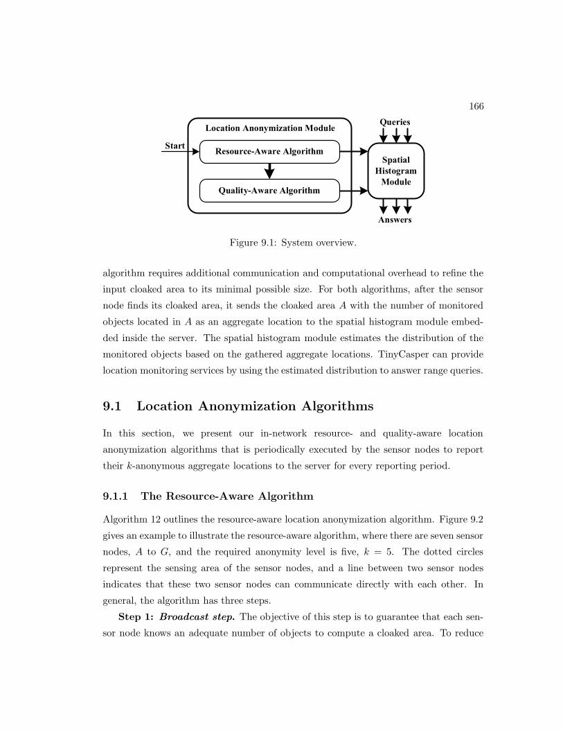
166

��

��

��

��

��

��

��

��

��

Figure 9.1: System overview.

algorithm requires additional communication and computational overhead to refine the

input cloaked area to its minimal possible size. For both algorithms, after the sensor

node finds its cloaked area, it sends the cloaked area A with the number of monitored

objects located in A as an aggregate location to the spatial histogram module embed-

ded inside the server. The spatial histogram module estimates the distribution of the

monitored objects based on the gathered aggregate locations. TinyCasper can provide

location monitoring services by using the estimated distribution to answer range queries.

9.1 Location Anonymization Algorithms

In this section, we present our in-network resource- and quality-aware location

anonymization algorithms that is periodically executed by the sensor nodes to report

their k-anonymous aggregate locations to the server for every reporting period.

9.1.1 The Resource-Aware Algorithm

Algorithm 12 outlines the resource-aware location anonymization algorithm. Figure 9.2

gives an example to illustrate the resource-aware algorithm, where there are seven sensor

nodes, A to G, and the required anonymity level is five, k = 5. The dotted circles

represent the sensing area of the sensor nodes, and a line between two sensor nodes

indicates that these two sensor nodes can communicate directly with each other. In

general, the algorithm has three steps.

Step 1: Broadcast step. The objective of this step is to guarantee that each sen-

sor node knows an adequate number of objects to compute a cloaked area. To reduce

167

��

��

� �

��

��

��

��

��

��

��

� �

��

��

��

��

� �

��

��

��

�

��

��

��

��

�

�

�

�

�

�

(a) PeerLists after the first broadcast

��

��

� �

��

��

��

��

� �

��

��

��

��

��

� �

��

��

� �

��

��

��

� �

��

��

��

�

��

��

��

� �

��

��

�

�

�

�

�

�

(b) Rebroadcast from sensor node F

��

��

� �

��

��

��

��

� �

��

��

��

��

��

� �

��

��

� �

��

��

��

� �

��

��

��

�

��

��

��

� �

��

��

�

�

�

�

�

�

(c) Resource-aware cloaked area of sensor node A

Figure 9.2: The resource-aware location anonymization algorithm (k = 5).

communication cost, this step relies on a heuristic that a sensor node only forwards

its received messages to its neighbors when some of them have not yet found an ade-

quate number of objects. In this step, after each sensor node m initializes an empty list

PeerList (Line 2 in Algorithm 12), m sends a message with its identity m.ID, sensing

area m.Area, and the number of objects located in its sensing area m.Count, to its neigh-

bors (Line 3). When m receives a message from a peer p, i.e., (p.ID, p.Area, p.Count),

m stores the message in its PeerList (Line 5). Whenever m finds an adequate number

of objects, m sends a notification message to its neighbors (Line 7). If m has not re-

ceived the notification message from all its neighbors, some neighbor has not found an

adequate number of objects; therefore m forwards the received message to its neighbors

168

Algorithm 12 Resource-aware Location Anonymization

1: function ResourceAware (Integer k, Sensor m, List R)2: PeerList ← {∅}

// Step 1: Broadcast step3: Send a message with m’s identity m.ID, sensing area m.Area, and object count m.Count to m’s

neighbor peers4: if Receive a message from a peer p, i.e., (p.ID, p.Area, p.count) then

5: Add the message to PeerList

6: if m has found an adequate number of objects then

7: Send a notification message to m’s neighbors8: end if

9: if Some m’s neighbor has not found an adequate number of objects then

10: Forward the message to m’s neighbors11: end if

12: end if

// Step 2: Cloaked area step13: S ← {m}14: Compute a score for each peer in PeerList

15: Repeatedly select the peer with the highest score from PeerList to S until the total number ofobjects in S is at least k

16: Area← a minimum bounding rectangle of the senor nodes in S17: N ← the total number of objects in S

// Step 3: Validation step18: if No containment relationship with Area and R ∈ R then

19: Send (Area,N) to the peers within Area and the server20: else if m’s sensing area is contained by some R ∈ R then

21: Randomly select a R′ ∈ R such that R′.Area contains m’s sensing area22: Send R′ to the peers within R′.Area and the server23: else

24: Send Area with a cloaked N to the peers within Area and the server25: end if

(Line 10).

Figures 9.2a and 9.2b illustrate the broadcast step. When a reporting period starts,

each sensor node sends a message with its identity, sensing area, and the number of

objects located in its sensing area to its neighbors. After the first broadcast, sensor

nodes A to F have found an adequate number of objects (represented by black circles),

as depicted in Figure 9.2a. Thus sensor nodes A to F send a notification message to their

neighbors. Since sensor node F has not received a notification message from its neighbor

G, F forwards its received messages, which include the information about sensor nodes

D and E, to G (Figures 9.2b). Finally, sensor node G has found an adequate number

of objects, so it sends a notification message to its neighbor, F . As all the sensor nodes

have found an adequate number of objects, they proceed to the next step.

169

Step 2: Cloaked area step. The basic idea of this step is that each sensor node

blurs its sensing area into a cloaked area that includes at least k objects, in order to

satisfy the k-anonymity privacy requirement. To minimize computational cost, this

step uses a greedy approach to find a cloaked area based on the information stored in

PeerList. For each sensor node m, m initializes a set S = {m}, and then determines a

score for each peer in its PeerList (Lines 13 to 14 in Algorithm 12). The score is defined

as a ratio of the object count of the peer to the Euclidean distance between the peer

and m. The idea behind the score is to select a set of peers from PeerList to S to form

a cloaked area that includes at least k objects and has an area as small as possible.

Then we repeatedly select the peer with the highest score from the PeerList to S until

S contains at least k objects (Line 15). Finally, m determines the cloaked area (Area)

that is a minimum bounding rectangle (MBR) that covers the sensing area of the sensor

nodes in S, and the total number of objects in S (N) (Lines 16 to 17).

An MBR is a rectangle with the minimum area (which is parallel to the axes) that

completely contains all desired regions, as illustrated in Figure 9.2c, where the dotted

rectangle is the MBR of the sensing area of sensor nodes A and B. The major reasons

of our algorithms aligning with MBRs rather than other polygons are that the concept

of MBRs have been widely adopted by existing query processing algorithms and most

database management systems have the ability to manipulate MBRs efficiently.

Figure 9.2c illustrates the cloaked area step. The PeerList of sensor node A contains

the information of three peers, B, D, and E. The object count of sensor nodes B, D,

and E is 3, 1, and 2, respectively. We assume that the distance from sensor node A to

sensor nodes B, D, and E is 17, 18, and 16, respectively. The score of B, D, and E is

3/17 = 0.18, 1/18 = 0.06, and 2/16 = 0.13, respectively. Since B has the highest score,

we select B. The sum of the object counts of A and B is six which is larger than the

required anonymity level k = 5, so we return the MBR of the sensing area of the sensor

nodes in S, i.e., A and B, as the resource-aware cloaked area of A, which is represented

by a dotted rectangle.

Step 3: Validation step. The objective of this step is to avoid reporting aggregate

locations with a containment relationship to the server. Let Ri and Rj be two aggregate

locations reported from sensor nodes i and j, respectively. If Ri’s monitored area

is included in Rj’s monitored area, Ri.Area ⊂ Rj .Area, or vice versa, Rj .Area ⊂

170

Ri.Area, they have a containment relationship. We do not allow the sensor nodes

to report their aggregate locations with the containment relationship to the server,

because combining these aggregate locations may pose privacy leakage. For example, if

Ri.Area ⊂ Rj .Area and Ri.Area 6= Rj .Area, an adversary can infer that the number

of objects residing in the non-overlapping area, Rj .Area − Ri.Area, is Rj .N − Ri.N .

In case that Rj.N − Ri.N < k, the adversary knows that the number of objects in

the non-overlapping is less than k, which violates the k-anonymity privacy requirement.

As this step ensures that no aggregate location with the containment relationship is

reported to the server, the adversary cannot obtain any deterministic information from

the aggregate locations.

In this step, each sensor node m maintains a list R to store the aggregate locations

sent by other peers. When a reporting period starts, m nullifies R. After m finds its

aggregate location Rm, m checks the containment relationship between Rm and the

aggregate locations in R. If there is no containment relationship between Rm and the

aggregate locations in R, m sends Rm to the peers within Rm.Area and the server

(Line 19 in Algorithm 12). Otherwise, m randomly selects an aggregate location Rp

from the set of aggregate locations in R that contain m’s sensing area, and m sends Rp

to the peers within Rp.Area and the server (Lines 21 to 22). In case that no aggregate

location in R contains m’s sensing area, we find a set of aggregate locations, R ′, in Rthat are contained by Rm and N ′ is the number of monitored persons in Rm that is

not covered by any aggregate location in R′. If N ′ ≥ k, the containment relationship

does not violate the k-anonymity privacy requirement; therefore m sends Rm to the

peers within Rm.Area and the server. However, if N ′ < k, m cloaks the number of

monitored persons of Rm, Rm.N , by increasing it by an integer uniformly selected

between k and 2k, and sends Rm to the peers within Rm.Area and the server (Line 24).

Since the server receives an aggregate location from each sensor node for every reporting

period, it cannot tell whether any containment relationship takes place among the actual

aggregate locations of the sensor nodes.

9.1.2 The Quality-Aware Algorithm

Algorithm 13 outlines the quality-aware algorithm that takes the cloaked area computed

by the resource-aware algorithm as an initial solution, and then refines it until the

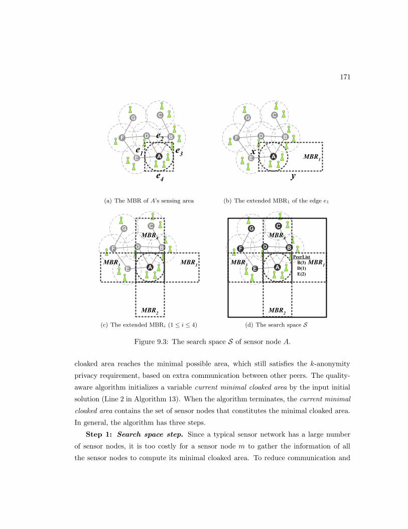
171

� �

�

�

�

�

�

��

��

��

��

(a) The MBR of A’s sensing area

� �

�

�

�

�

�

�

�

��

(b) The extended MBR1 of the edge e1

� �

�

�

�

�

�

��

��

��

��

(c) The extended MBRi (1 ≤ i ≤ 4)

��

��

� �

��

� �

�

�

�

�

�

��

��

��

��

(d) The search space S

Figure 9.3: The search space S of sensor node A.

cloaked area reaches the minimal possible area, which still satisfies the k-anonymity

privacy requirement, based on extra communication between other peers. The quality-

aware algorithm initializes a variable current minimal cloaked area by the input initial

solution (Line 2 in Algorithm 13). When the algorithm terminates, the current minimal

cloaked area contains the set of sensor nodes that constitutes the minimal cloaked area.

In general, the algorithm has three steps.

Step 1: Search space step. Since a typical sensor network has a large number

of sensor nodes, it is too costly for a sensor node m to gather the information of all

the sensor nodes to compute its minimal cloaked area. To reduce communication and

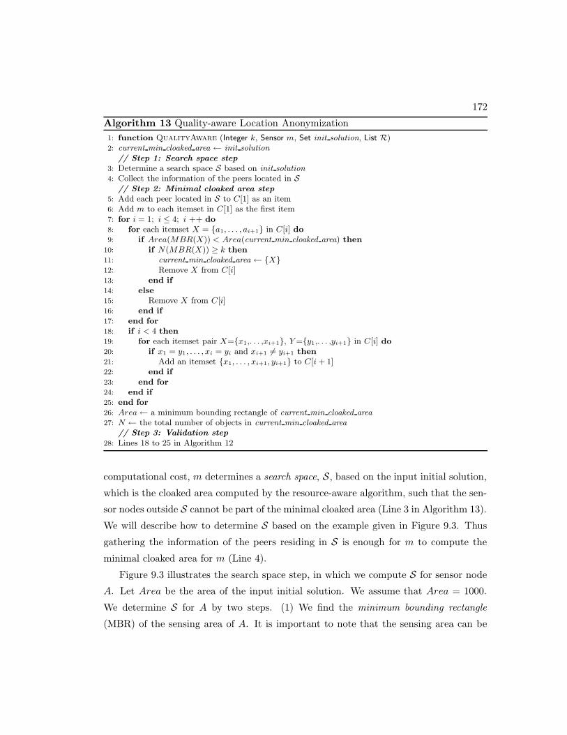
172

Algorithm 13 Quality-aware Location Anonymization

1: function QualityAware (Integer k, Sensor m, Set init solution, List R)2: current min cloaked area ← init solution

// Step 1: Search space step3: Determine a search space S based on init solution

4: Collect the information of the peers located in S// Step 2: Minimal cloaked area step

5: Add each peer located in S to C[1] as an item6: Add m to each itemset in C[1] as the first item7: for i = 1; i ≤ 4; i ++ do

8: for each itemset X = {a1, . . . , ai+1} in C[i] do

9: if Area(MBR(X)) < Area(current min cloaked area) then

10: if N(MBR(X)) ≥ k then

11: current min cloaked area ← {X}12: Remove X from C[i]13: end if

14: else

15: Remove X from C[i]16: end if

17: end for

18: if i < 4 then

19: for each itemset pair X={x1,. . . ,xi+1}, Y ={y1,. . . ,yi+1} in C[i] do

20: if x1 = y1, . . . , xi = yi and xi+1 6= yi+1 then

21: Add an itemset {x1, . . . , xi+1, yi+1} to C[i + 1]22: end if

23: end for

24: end if

25: end for

26: Area← a minimum bounding rectangle of current min cloaked area

27: N ← the total number of objects in current min cloaked area

// Step 3: Validation step28: Lines 18 to 25 in Algorithm 12

computational cost, m determines a search space, S, based on the input initial solution,

which is the cloaked area computed by the resource-aware algorithm, such that the sen-

sor nodes outside S cannot be part of the minimal cloaked area (Line 3 in Algorithm 13).

We will describe how to determine S based on the example given in Figure 9.3. Thus

gathering the information of the peers residing in S is enough for m to compute the

minimal cloaked area for m (Line 4).

Figure 9.3 illustrates the search space step, in which we compute S for sensor node

A. Let Area be the area of the input initial solution. We assume that Area = 1000.

We determine S for A by two steps. (1) We find the minimum bounding rectangle

(MBR) of the sensing area of A. It is important to note that the sensing area can be

173

in any polygon or irregular shape. In Figure 9.3a, the MBR of the sensing area of A is

represented by a dotted rectangle, where the edges of the MBR are labeled by e1 to e4.

(2) For each edge ei of the MBR, we compute an MBRi by extending the opposite edge

such that the area of the extended MBRi is equal to Area. S is the MBR of the four

extended MBRi. Figure 9.3b depicts the extended MBR1 of the edge e1 by extending

the opposite edge e3, where MBR1.x is the length of MBR1, MBR1.y = Area/MBR1.x

and Area = 1000. Figure 9.3c shows the four extended MBRs, MBR1 to MBR4, which

are represented by dotted rectangles. The MBR of the four extended MBRs constitutes

S, which is represented by a rectangle (Figure 9.3d). Finally, the sensor node only needs

the information of the peers within S.

Step 2: Minimal cloaked area step. This step takes a set of peers residing in

the search space, S, as an input and computes the minimal cloaked area for the sensor

node m. Although the search space step already prunes the entire system space into S,

exhaustively searching the minimal cloaked area among the peers residing in S, which

needs to search all the possible combinations of these peers, could still be costly. Thus

we propose two optimization techniques to reduce computational cost.

The basic idea of the first optimization technique is that we do not need to examine

all the combinations of the peers in S; instead, we only need to consider the combinations

of at most four peers. The rationale behind this optimization is that an MBR is defined

by at most four sensor nodes because at most two sensor nodes define the width of the

MBR (parallel to the x-axis) while at most two other sensor nodes define the height of the

MBR (parallel to the y-axis). Thus this optimization mainly reduces computational cost

by reducing the number of MBR computations among the peers in S. The correctness

of this optimization technique will be discussed in Section 9.1.2.

The second optimization technique has two properties, lattice structure and mono-

tonicity property. We first describe these two properties, and then present a progressive

refinement approach for finding a minimal cloaked area.

A. Lattice structure. In a lattice structure, a data set that contains n items can

generate 2n−1 itemsets excluding a null set. In the sequel, since the null set is meaning-

less to our problem, it will be neglected. Figure 9.4 shows the lattice structure of a set

of four items S = {s1, s2, s3, s4}, where each black line between two itemsets indicates

that an itemset at a lower level is a subset of an itemset at a higher level. For our

174

��

��

��

��

��

��

��

��

��

��

��

��

��

��

��

��

��

��

��

��

��

��

Figure 9.4: The lattice structure of a set of four items.

problem, given a set of sensor nodes S = {s1, s2, . . . , sn}, all the possible combinations

of these sensor nodes are the non-empty subsets of S; thus we can use a lattice structure

to generate the combinations of the sensor nodes in S. In the lattice structure, since

each itemset at level i has i items in S, each combination at the lowest level, level 1,

contains a distinct item in S; therefore there are n itemsets at the lowest level. We

generate the lattice structure from the lowest level based on a simple generation rule:

given two sorted itemsets X = {x1, . . . , xi} and Y = {y1, . . . , yi} in increasing order,

where each itemset has i items (1 ≤ i < n), if all item pairs but the last one in X and

Y are the same, x1 = y1, x2 = y2, . . ., xi−1 = yi−1, and xi 6= yi, we generate a new

itemset with i + 1 items, {x1, . . . , xi, yi}. In the example, we use bold lines to illustrate

the construction of the lattice structure based on the generation rule. For example, the

itemset {s1, s2, s3, s4} at level 4 is combined by the itemsets {s1, s2, s3} and {s1, s2, s4}at level 3, so there is a bold line from {s1, s2, s3, s4} to {s1, s2, s3} and another one to

{s1, s2, s4}.B. Monotonicity property. Let S be a set of items, and P be the power set of

S, 2S . The monotonicity property of a function f indicates that if X is a subset of Y ,

then f(X) must not exceed f(Y ), i.e., ∀X,Y ∈ P : (X ⊆ Y )→ f(X) ≤ f(Y ). For our

problem, the MBR of a set of sensor nodes S has the monotonicity property, because

adding sensor nodes to S must not decrease the area of the MBR of S or the number

175

��

��

��

��

��

(a) The full lattice structure

��

��

��

��

��

��

(b) Pruning itemset {A, B}

��

��

��

��

��

��

(c) Pruning itemset {A, D}

��

��

��

��

��

��

(d) The minimal cloaked area

Figure 9.5: The quality-aware cloaked area of sensor node A.

of objects within the MBR of S. Let Area(MBR(X)) and N(MBR(X)) be two func-

tions that return the area of the MBR of an itemset X and the number of monitored

objects located in the MBR, respectively. Thus, given two itemsets X and Y , if X ⊆ Y ,

then Area(MBR(X)) ≤ Area(MBR(Y )) and N(MBR(X)) ≤ N(MBR(Y )). By this

property, we propose two pruning conditions in the lattice structure. (1) If a combina-

tion C gives the current minimal cloaked area, other combinations that contain C at the

higher levels of the lattice structure should be pruned. This is because the monotonic-

ity property indicates that the pruned combinations cannot constitute a cloaked area

smaller than the current minimal cloaked area. (2) Similarly, if a combination C consti-

tutes a cloaked area that is the same or larger than the current minimal cloaked area,

other combinations that contain C at the higher levels of the lattice structure should be

176

pruned.

C. Progressive refinement. Since the monotonicity property shows that we would

not need to generate a complete lattice structure to compute a minimal cloaked area,

we generate the lattice structure of the peers in the search space, S, progressively from

the lowest level of the lattice structure to its higher levels, in order to minimize the

computational and storage overhead. To compute the minimal cloaked area for the

sensor node m, we first generate an itemset for each peer in S at the lowest level of the

lattice structure, C[1] (Line 5 in Algorithm 13). To accommodate with our problem,

we add m to each itemset in C[1] as the first item (Line 6). Such accommodation does

not affect the generation of the lattice structure, but each itemset has an extra item,

m. For each itemset X in C[1], we determine the MBR of X, MBR(X). If the area of

MBR(X) is less than the current minimal cloaked area and the total number of objects

in MBR(X) is at least k, we set X to the current minimal cloaked area, and remove X

from C[1] based on the first pruning condition of the monotonicity property (Lines 11

to 12). However, if the area of MBR(X) is equal to or larger than the area of the

current minimal cloaked area, we also remove X from C[1] based on the second pruning

condition of the monotonicity property (Line 15). Then we generate the itemsets, where

each itemset contains two items, at the second lowest level of the lattice structure, C[2],

based on the remaining itemsets in C[1] based on the generation rule of the lattice

structure. We repeat this procedure until we produce the itemsets at the highest level

of the lattice structure, C[4], or all the itemsets at the current level are pruned (Lines 19

to 23). After we examine all non-pruned itemsets in the lattice structure, the current

minimal cloaked area stores the combination giving the minimal cloaked area (Lines 26

to 27).

Figure 9.5 illustrates the minimal cloaked area step that computes the minimal

cloaked area for sensor node A. The set of peers residing in the search space is S =

{B,D,E}. We assume that the area of the MBR of {A,B}, {A,D}, and {A,E} is

1000, 1200, and 900, respectively. The number of objects residing in the MBR of

{A,B}, {A,D}, and {A,E} is six, four, and five, respectively, as depicted in Figure 9.2.

Figure 9.5a depicts the full lattice structure of S where A is added to each itemset as the

first item. Initially, the current minimal cloaked area is set to the initial solution, which

is the MBR of {A,B} ’computed by the resource-aware algorithm. The area of the MBR

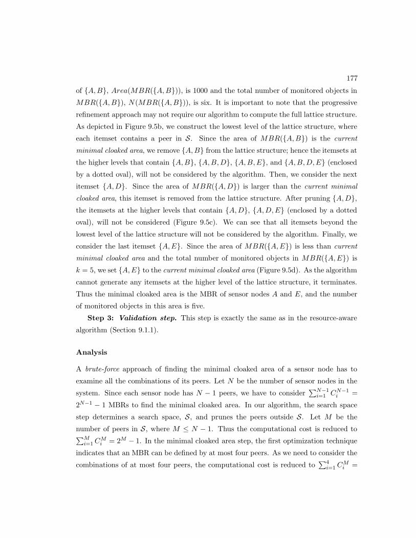
177

of {A,B}, Area(MBR({A,B})), is 1000 and the total number of monitored objects in

MBR({A,B}), N(MBR({A,B})), is six. It is important to note that the progressive

refinement approach may not require our algorithm to compute the full lattice structure.

As depicted in Figure 9.5b, we construct the lowest level of the lattice structure, where

each itemset contains a peer in S. Since the area of MBR({A,B}) is the current

minimal cloaked area, we remove {A,B} from the lattice structure; hence the itemsets at

the higher levels that contain {A,B}, {A,B,D}, {A,B,E}, and {A,B,D,E} (enclosed

by a dotted oval), will not be considered by the algorithm. Then, we consider the next

itemset {A,D}. Since the area of MBR({A,D}) is larger than the current minimal

cloaked area, this itemset is removed from the lattice structure. After pruning {A,D},the itemsets at the higher levels that contain {A,D}, {A,D,E} (enclosed by a dotted

oval), will not be considered (Figure 9.5c). We can see that all itemsets beyond the

lowest level of the lattice structure will not be considered by the algorithm. Finally, we

consider the last itemset {A,E}. Since the area of MBR({A,E}) is less than current

minimal cloaked area and the total number of monitored objects in MBR({A,E}) is

k = 5, we set {A,E} to the current minimal cloaked area (Figure 9.5d). As the algorithm

cannot generate any itemsets at the higher level of the lattice structure, it terminates.

Thus the minimal cloaked area is the MBR of sensor nodes A and E, and the number

of monitored objects in this area is five.

Step 3: Validation step. This step is exactly the same as in the resource-aware

algorithm (Section 9.1.1).

Analysis

A brute-force approach of finding the minimal cloaked area of a sensor node has to

examine all the combinations of its peers. Let N be the number of sensor nodes in the

system. Since each sensor node has N − 1 peers, we have to consider∑N−1

i=1 CN−1i =

2N−1 − 1 MBRs to find the minimal cloaked area. In our algorithm, the search space

step determines a search space, S, and prunes the peers outside S. Let M be the

number of peers in S, where M ≤ N − 1. Thus the computational cost is reduced to∑M

i=1 CMi = 2M − 1. In the minimal cloaked area step, the first optimization technique

indicates that an MBR can be defined by at most four peers. As we need to consider the

combinations of at most four peers, the computational cost is reduced to∑4

i=1 CMi =

178

(M4 − 2M3 + 11M2 + 14M)/24 = O(M 4). Furthermore, the second optimization

technique uses the monotonicity property to prune the combinations, which cannot

give the minimal cloaked area. In our example, the brute-force approach considers all

the combinations of six peers; hence this approach computes 26 − 1 = 63 MBRs to

find the minimal cloaked area of sensor node A. In our algorithm, the search space

step reduces the entire space into S, which contains only three peers; hence this step

needs to compute 23 − 1 = 7 MBRs. After examining the three itemsets at the lowest

level of the lattice structure, all other itemsets at the higher levels are pruned. Thus

the progressive refinement approach considers only three combinations. Therefore our

algorithm reduces over 95% computational cost of the brute-force approach, as it reduces

the number of MBR computations from 63 to 3.


In this section, we show the correctness of the quality-aware location anonymization

algorithm.

Theorem 10. Given a resource-aware cloaked area of size Area of a sensor node s, a

search space, S, computed by the quality-aware algorithm contains the minimal cloaked

area.

Proof. Let X be the minimal cloaked area of size equal to or less than Area. We know

that X must totally cover the sensing area of s. Suppose X is not totally covered by

S, X must contain at least one extended MBR, MBRi, where 1 ≤ i ≤ 4 (Figure 9.3c).

This means that the area of X is larger than the area of an extended MBR, Area. This

contradicts to the assumption that X is the minimal cloaked area; thus X is included

in S.

Theorem 11. A minimum bounding rectangle (MBR) can be defined by at most four

sensor nodes.

Proof. By definition, given an MBR, each edge of the MBR touches the sensing area

of some sensor node. In an extreme case, there is a distinct sensor node touching each

edge of the MBR but not other edges. The MBR is defined by four sensor nodes, which

touch different edges of the MBR. For any edge e of the MBR, if multiple sensor nodes

179

touch e but not other edges, we can simply pick one of these sensor nodes, because any

one of these sensor nodes gives the same e. Thus an MBR is defined by at most four

sensor nodes.

9.2 Spatial Histogram

In this section, we present a spatial histogram that is embedded inside the server to esti-

mate the distribution of the monitored objects based on the aggregate locations reported

from the sensor nodes. Our spatial histogram is represented by a two-dimensional array

that models a grid structure G of NR rows and NC columns; hence, the system space

is divided into NR × NC disjoint equal-sized grid cells. In each grid cell G(i, j), we

maintain a float value that acts as an estimator H[i, j] (1 ≤ i ≤ NC , 1 ≤ j ≤ NR) of

the number of objects within its area. We assume that the system has the ability to

know the total number of moving objects M in the system. The value of M will be

used to initialize the spatial histogram. In practice, M can be computed online for both

indoor and outdoor dynamic environments. For the indoor environment, the sensor

nodes can be deployed at each entrance and exit to count the number of users entering

or leaving the system [117, 118]. For the outdoor environment, the sensor nodes have

been already used to count the number of people in a predefined area [119]. We use the

spatial histogram to provide approximate location monitoring services. The accuracy

of the spatial histogram, which indicates the utility of our privacy-preserving location

monitoring system, will be evaluated in Section 9.4.

Algorithm 14 outlines the maintenance of our spatial histogram. Initially, we assume

that the objects are evenly distributed in the system, so the estimated number of objects

within each grid cell is H[i, j] = M/(NR × NC). The input of the histogram is a set

of aggregate locations R reported from the sensor nodes. Each aggregate location R

in R contains a cloaked area, R.Area, and the number of monitored objects within

R.Area, R.N . First, the aggregate locations in R are grouped into the same partition

P = {R1, R2, . . . , R|P |} if their cloaked areas are not overlapping with each other, which

means that for every pair of aggregate locations Ri and Rj in P , Ri.Area∩Rj .Area = ∅(Lines 2 to 8). Then, for each partition P , we update its entire set of aggregate locations

to the spatial histogram at the same time. For each aggregate location R in P , we

180

Algorithm 14 Spatial Histogram Maintenance

1: function HistogramMaintenance (AggregateLocationSet R)2: for each aggregate location R ∈ R do

3: if there is an existing partition P = {R1, . . . , R|P |} such that R.Area ∩ Rk.Area = ∅ for everyRk ∈ P then

4: Add R to P5: else

6: Create a new partition for R7: end if

8: end for

9: for each partition P do

10: for each aggregate location Rk ∈ P do

11: Rk.N ←∑

G[i,j]∈Rk.AreaH[i, j]

12: For every cell G(i, j) ∈ Rk.Area, H[i, j]← Rk.N

No. of cells within Rk .Area

13: end for

14: P.Area← R1.Area ∪ . . . ∪R|P |.Area15: For every cell G(i, j) /∈ P.Area,

H[i, j] = H[i, j] +∑

Rk∈P

Rk.N−Rk .N

No. of cells outside P.Area

16: end for

record the estimation error, which is the difference between the sum of the estimators

within R.Area, R.N , and R.N , and then R.N is uniformly distributed among the

estimators within R.Area; hence each estimator within R.Area is set to R.N divided

by the total number of grid cells within R.Area (Lines 10 to 13). After processing

all the aggregate locations in P , we sum up the estimation error of each aggregate

location in P ,∑|P |

k=1 Rk.N −Rk.N , that is uniformly distributed among the estimators

outside P.Area, where P.Area is the area covered by some aggregate location in P ,

P.Area = ∪Rk∈P Rk.Area (Line 15). Formally, for each partition P that contains |P |aggregate locations Rk (1 ≤ k ≤ |P |), every estimator in the histogram is updated as

follows:

H[i, j] =

Rk.NNo. of cells within Rk.Area

, for G(i, j) ∈ Rk.Area

H[i, j] +∑|P |

k=1 Rk .N−Rk.N

No. of cells outside P.Area, for G(i, j) /∈ P.Area

Example. Figure 9.6 depicts an example of maintaining the spatial histogram in

which the grid structure G divides the system space into NR × NC = 5 × 5 grid cells.

When the spatial histogram is initialized, the total number of objects in the system

is M = 100; and hence, the estimator of each grid cell is initially set to M/(NR ×

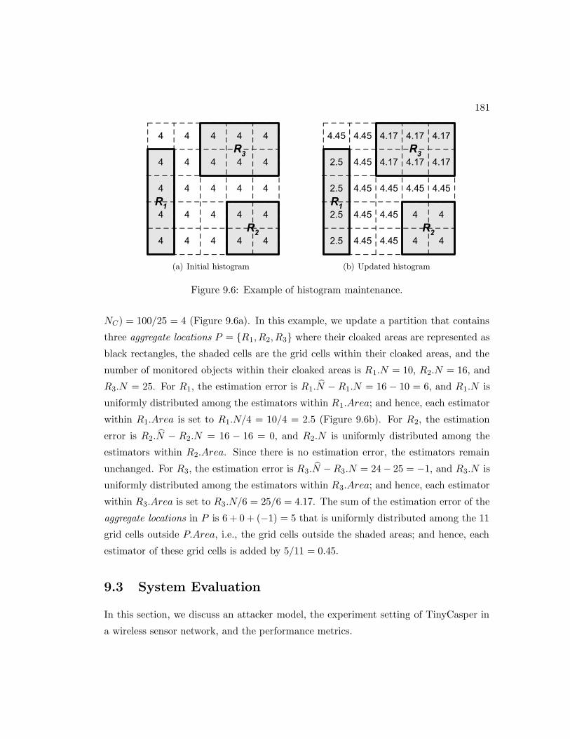
181

� � � � �

� � � � �

� � � � �

� � � � �

� � � � �

��

��

��

(a) Initial histogram

��

��

��

��

��

��

��

��

(b) Updated histogram

Figure 9.6: Example of histogram maintenance.

NC) = 100/25 = 4 (Figure 9.6a). In this example, we update a partition that contains

three aggregate locations P = {R1, R2, R3} where their cloaked areas are represented as

black rectangles, the shaded cells are the grid cells within their cloaked areas, and the

number of monitored objects within their cloaked areas is R1.N = 10, R2.N = 16, and

R3.N = 25. For R1, the estimation error is R1.N − R1.N = 16 − 10 = 6, and R1.N is

uniformly distributed among the estimators within R1.Area; and hence, each estimator

within R1.Area is set to R1.N/4 = 10/4 = 2.5 (Figure 9.6b). For R2, the estimation

error is R2.N − R2.N = 16 − 16 = 0, and R2.N is uniformly distributed among the

estimators within R2.Area. Since there is no estimation error, the estimators remain

unchanged. For R3, the estimation error is R3.N −R3.N = 24− 25 = −1, and R3.N is

uniformly distributed among the estimators within R3.Area; and hence, each estimator

within R3.Area is set to R3.N/6 = 25/6 = 4.17. The sum of the estimation error of the

aggregate locations in P is 6 + 0 + (−1) = 5 that is uniformly distributed among the 11

grid cells outside P.Area, i.e., the grid cells outside the shaded areas; and hence, each

estimator of these grid cells is added by 5/11 = 0.45.

9.3 System Evaluation

In this section, we discuss an attacker model, the experiment setting of TinyCasper in

a wireless sensor network, and the performance metrics.

182

9.3.1 Attacker Model

To evaluate the privacy protection of TinyCasper, we simulate an attacker attempting

to infer the number of objects residing in a sensor node’s sensing area. We will analyze

the evaluation result in Section 9.4.1. The key idea of the attacker model is that if the

attacker cannot infer the exact object count of the sensor node from our system output,

the attacker cannot infer the location information corresponding to an individual object.

We consider the worst-case scenario where the attacker has the background knowledge

about the system, which includes the map layout of the system, the location of each

sensor node, the sensing area of each sensor node, the total number of objects currently

residing in the system, and the aggregate locations reported from the sensor nodes. In

general, the attacker model is defined as: Given an area A (that corresponds to the mon-

itored area of a sensor node) and a set of aggregate locations R = {R1, R2, . . . , R|R|}overlapping with A, the attacker estimates the number of persons within A. Since the

validation step in our location anonymization algorithms guarantees that the contain-

ment relationship among the aggregate locations reported to the server does not violate

the k-anonymity privacy requirement, we do not consider any containment relationship

in R.

Without loss of generality, we use the Poisson distribution as a concrete exemplary

distribution for the attacker model [120]. Under the Poisson distribution, objects are

uniformly distributed in an area within intensity of λ. The probability of n distinct

objects in a region S of size s is P (N(S) = n) = e−λs(λs)n

n! , where λ is computed as the

number of objects in the system divided by the area of the system.

Suppose that the object count of each aggregate location Ri is ni, where 1 ≤ i ≤ |R|,and the aggregate locations in R and A constitute m non-overlapping subregions Sj ,

where 1 ≤ j ≤ m; hence N(Ri) =∑

Sj∈RiN(Sj) = ni. Each subregion must either

intersect or not intersect A, and it intersects one or more aggregate locations. If a

subregion Sk intersects A, but none of the aggregate locations in R, then N(Sk) = 0.

The probability mass function of the number of distinct objects in A being equal to na,

N = na, given the aggregate locations in R can be expressed as follows:

183

P (N = na|N(R1) = n1, . . . , N(R|R|) = n|R|)

=P (N = na, N(R1) = n1, . . . , N(R|R|) = n|R|)

P (N(R1) = n1, . . . , N(R|R|) = n|R|)

=

∑Vi∈(VS∩VA) < vi

1, vi2, . . . , v

im >

∑Vj∈VS

< vj1, v

j2, . . . , v

jm >

, (9.1)

where the notation V =< v1, v2, . . . , vm > represents the joint probability that there

are vi objects in a subregion Si (1 ≤ i ≤ m); the joint probability is computed

as∏

1≤i≤m P (N(Si) = vi). The lower and upper bounds of vi (denoted as LB(vi)

and UB(vi), respectively) are zero and the minimum nj of the aggregate locations

intersecting Si, respectively. Thus the possible value of vi is within a range of

[0,minRj∩Si 6=∅∧1≤i≤m∧1≤j≤|R|(nj)]. VS is the set of < v1, v2, . . . , vm > that is a solution

to the following equations: VS :∑

Si∈R1vi = n1,

∑Si∈R2

vi = n2, . . . ,∑

Si∈R|R|vi =

n|R|, where vi ≥ 0 for 1 ≤ i ≤ m. VA is the set of < v1, v2, . . . , vm > that satisfies the

following equation: VA :∑

1≤i≤m vi = na.

The attacker uses an exhaustive approach to find all possible solutions to VS , in

order to compute the expected value E(N ) of Equation 9.1 as the estimated value of

na. The complexity of computing E(N ) is O(∏

1≤i≤m UB(vi)). Since the complexity of

the attacker model is an exponential function of m and m would be much larger than

|R|, such exponential complexity makes it prohibitive for the attacker model to be used

to provide online location monitoring services; therefore we use our spatial histogram to

provide online services in the experiments. We will evaluate the resilience of our system

to the attacker model in Section 9.4.1.

9.3.2 Simulation Settings

In all experiments, we simulate 30 × 30 sensor nodes that are uniformly distributed in

a 600 × 600 system space. Each sensor node is responsible for monitoring a 20 × 20

space. We generate a set of moving objects that freely roam around the system space.

Unless mentioned otherwise, the experiments consider 5,000 moving objects that move

at a random speed within a range of [0, 5] space unit(s) per time unit, and the required

anonymity level is k = 20. The spatial histogram contains NR × NC = 200 × 200 grid

184


Description Default Value Range

Histogram size (NR ×NC) 200 × 200 502 to 2502

Query region size ratio [0.001, 0.032] 0.001 to 0.256Number of moving objects 5,000 2,000 to 10,000

k-anonymity level 20 10 to 30Object mobility speed [0,5] [0,5] to [0,30]

cells, and we issue 1,000 range queries whose query region size is specified by a ratio of

the query region area to the system area, that is, a query region size ratio. The default

query region size ratio is uniformly selected within a range of [0.001, 0.032]. Table 9.1

gives a summary of the parameter settings.

9.3.3 Performance Metrics

We evaluate TinyCasper in terms of five performance metrics. (1) Attack model error.

This metric measures the resilience of our system to the attacker model by the relative

error between the estimated number of objects N in a sensor node’s sensing area and

the actual one N . The error is measured as |N−N |N

. When N = 0, we consider N

as the error. (2) Communication cost. We measure the communication cost of our

location anonymization algorithms in terms of the average number of bytes sent by each

sensor node per reporting period. This metric also indicates the network traffic and the

power consumption of the sensor nodes. (3) Cloaked area size. This metric measures

the quality of the aggregate locations reported by the sensor nodes. The smaller the

cloaked area, the better the accuracy of the aggregate location is. (4) Computational

cost. We measure the computational cost of our location anonymization algorithms in

terms of the average number of minimum bounding rectangle (MBR) computations that

are needed to determine a resource- or quality-aware cloaked area. We compare our

algorithms with a basic approach that computes the MBR for each combination of the

peers in the required search space to find the minimal cloaked area. The basic approach

does not employ any optimization techniques proposed for our quality-aware algorithm.

(5) Query error. This metric measures the utility of our system, in terms of the relative

185

0

0.1

0.2

0.3

0.4

0.5

0.6

0.7

10 15 20 25 30

Att

ack

Mod

el E

rror

Anonymity Levels

Resource-AwareQuality-Aware

(a) Anonymity levels

0

0.1

0.2

0.3

0.4

0.5

0.6

0.7

2 4 6 8 10

Att

ack

Mod

el E

rror

Number of Objects (in thousands)


(b) Number of objects

Figure 9.7: Attacker model error.

error between the query answer M , which is the estimated number of objects within

the query region based on a spatial histogram, and the actual answer M , respectively.

The error is measured as |M−M |M

. When M = 0, we consider M as the error.

9.4 Experimental Results and Analysis

In this section, we show and analyze the experimental results with respect to the privacy

protection and the quality of location monitoring services of TinyCasper.

9.4.1 Anonymization Strength

Figure 9.7 depicts the resilience of our system to the attacker model with respect to

the anonymity level and the number of objects. In the figure, the performance of the

resource- and quality-aware algorithms is represented by black and gray bars, respec-

tively. Figure 9.7a depicts that the stricter the anonymity level, the larger the attacker

model error will be encountered by an adversary. When the anonymity level gets stricter,

our algorithms generate larger cloaked areas, which reduce the accuracy of the aggre-

gate locations reported to the server. Figure 9.7b shows that the attacker model error

reduces, as the number of objects gets larger. This is because when there are more

objects, our algorithms generate smaller cloaked areas, which increase the accuracy of

the aggregate locations reported to the server. It is difficult to set a hard quantitative

186

0

0.1

0.2

0.3

0.4

0.5

0.6

0.7

0.8

0.001 0.002 0.004 0.008 0.016 0.032 0.064 0.128 0.256

Que

ry A

nsw

er E

rror

Query Region Size Ratio

k=10k=15k=20k=25k=30

(a) Resource-aware algorithm

0

0.1

0.2

0.3

0.4

0.5

0.6

0.001 0.002 0.004 0.008 0.016 0.032 0.064 0.128 0.256

Que

ry A

nsw

er E

rror

Query Region Size Ratio

k=10k=15k=20k=25k=30

(b) Quality-aware algorithm

Figure 9.8: Query region size.

threshold for the attacker model error. However, it is evident that the adversary cannot

infer the number of objects in the sensor node’s sensing area with any fidelity.

9.4.2 Effect of Query Region Size

Figure 9.8 depicts the privacy protection and the quality of our location monitoring

system with respect to increasing the query region size ratio from 0.001 to 0.256, where

the query region size ratio is the ratio of the query region area to the system area

and the query region size ratio 0.001 corresponds to the size of a sensor node’s sensing

area. The results give evidence that our system provides low quality location monitoring

services for the range query with a small query region, and better quality services for

larger query regions. This is an important feature to protect personal location privacy,

187

3

4

5

6

7

8

9

10

2 4 6 8 10

Num

ber

of B

ytes

(in

thou

sand

s)



(a) Communication cost

0

0.5

1

1.5

2

2.5

100 200 300 400 500

Ave

rage

Clo

aked

Are

a S

ize

(km

2 )

No. of Users (K)

(b) Cloaked area size

10-1100101102103104105106107108

2 4 6 8 10

No.

of M

BR

Com

puta

tions



Basic

(c) Computational cost

0

0.05

0.1

0.15

0.2

0.25

2 4 6 8 10

Que

ry A

nsw

er E

rror



(d) Estimation error

Figure 9.9: Number of objects.

because providing the accurate number of objects in a small area could reveal individual

location information; therefore an adversary cannot use our system output to track the

monitored objects with any fidelity. The definition of a small query region is relative to

the required anonymity level k. For example, we want to provide low quality services,

such that the query error is at least 0.2, for small query regions. For the resource-aware

algorithm, Figure 9.8a shows that when k = 10, a query region is said to be small if its

query region size is not larger than 0.002 (it is about two sensor nodes’ sensing area).

However, when k = 30, a query region is only considered as small if its query region size

is not larger than 0.016 (it is about 16 sensor nodes’ sensing area). For the quality-aware

algorithm, Figure 9.8b shows that when k = 10, a query region is said to be small if

188

3 4 5 6 7 8 9

10 11 12 13

10 15 20 25 20

Num

ber

of B

ytes

(in

thou

sand

s)

Anonymity Levels



0.5

1

1.5

2

2.5

3

3.5

100 150 200 250 300

Ave

rage

Clo

aked

Are

a S

ize

(km

2 )

Anonymity Levels


10-1100101102103104105106107108109

10 15 20 25 30

No.

of M

BR

Com

puta

tions

Anonymity Levels


Basic


0

0.05

0.1

0.15

0.2

0.25

0.3

10 15 20 25 30

Que

ry A

nsw

er E

rror

Anonymity Levels



Figure 9.10: Anonymity levels.

its query region size is not larger than 0.002, while when k = 30, a query region is only

considered as small if its query region size is not larger than 0.004. The results also

show that the quality-aware algorithm always performs better than the resource-aware

algorithm.

9.4.3 Effect of the Number of Objects

Figure 9.9 depicts the performance of our system with respect to increasing the number

of objects from 2,000 to 10,000. Figure 9.9a shows that when the number of objects

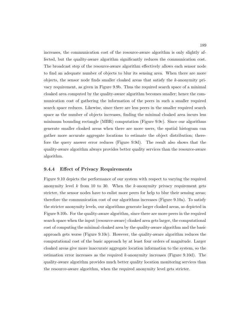
189

increases, the communication cost of the resource-aware algorithm is only slightly af-

fected, but the quality-aware algorithm significantly reduces the communication cost.

The broadcast step of the resource-aware algorithm effectively allows each sensor node

to find an adequate number of objects to blur its sensing area. When there are more

objects, the sensor node finds smaller cloaked areas that satisfy the k-anonymity pri-

vacy requirement, as given in Figure 9.9b. Thus the required search space of a minimal

cloaked area computed by the quality-aware algorithm becomes smaller; hence the com-

munication cost of gathering the information of the peers in such a smaller required

search space reduces. Likewise, since there are less peers in the smaller required search

space as the number of objects increases, finding the minimal cloaked area incurs less

minimum bounding rectangle (MBR) computation (Figure 9.9c). Since our algorithms

generate smaller cloaked areas when there are more users, the spatial histogram can

gather more accurate aggregate locations to estimate the object distribution; there-

fore the query answer error reduces (Figure 9.9d). The result also shows that the

quality-aware algorithm always provides better quality services than the resource-aware

algorithm.


Figure 9.10 depicts the performance of our system with respect to varying the required

anonymity level k from 10 to 30. When the k-anonymity privacy requirement gets

stricter, the sensor nodes have to enlist more peers for help to blur their sensing areas;

therefore the communication cost of our algorithms increases (Figure 9.10a). To satisfy

the stricter anonymity levels, our algorithms generate larger cloaked areas, as depicted in

Figure 9.10b. For the quality-aware algorithm, since there are more peers in the required

search space when the input (resource-aware) cloaked area gets larger, the computational

cost of computing the minimal cloaked area by the quality-aware algorithm and the basic

approach gets worse (Figure 9.10c). However, the quality-aware algorithm reduces the

computational cost of the basic approach by at least four orders of magnitude. Larger

cloaked areas give more inaccurate aggregate location information to the system, so the

estimation error increases as the required k-anonymity increases (Figure 9.10d). The

quality-aware algorithm provides much better quality location monitoring services than

the resource-aware algorithm, when the required anonymity level gets stricter.

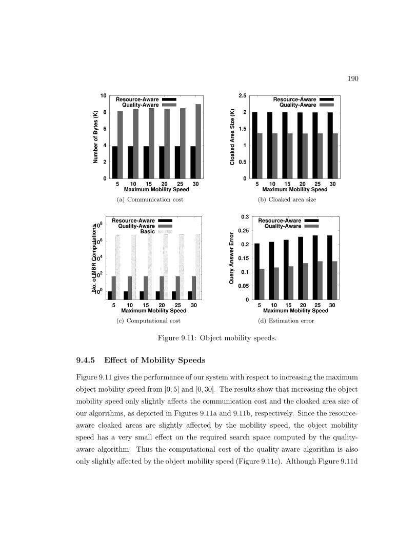
190

0

2

4

6

8

10

5 10 15 20 25 30

Num

ber

of B

ytes

(K)

Maximum Mobility Speed



0

0.5

1

1.5

2

2.5

5 10 15 20 25 30

Clo

aked

Are

a S

ize

(K)




100

102

104

106

108

5 10 15 20 25 30

No.

of M

BR

Com

puta

tions



Basic


0

0.05

0.1

0.15

0.2

0.25

0.3

5 10 15 20 25 30

Que

ry A

nsw

er E

rror




Figure 9.11: Object mobility speeds.

9.4.5 Effect of Mobility Speeds

Figure 9.11 gives the performance of our system with respect to increasing the maximum

object mobility speed from [0, 5] and [0, 30]. The results show that increasing the object

mobility speed only slightly affects the communication cost and the cloaked area size of

our algorithms, as depicted in Figures 9.11a and 9.11b, respectively. Since the resource-

aware cloaked areas are slightly affected by the mobility speed, the object mobility

speed has a very small effect on the required search space computed by the quality-

aware algorithm. Thus the computational cost of the quality-aware algorithm is also

only slightly affected by the object mobility speed (Figure 9.11c). Although Figure 9.11d

191

shows that query answer error gets worse when the objects are moving faster, the query

accuracy of the quality-aware algorithm is consistently better than the resource-aware

algorithm.

9.5 Summary

In this chapter, we present the TinyCasper system; a privacy-preserving location moni-

toring system designed for wireless sensor networks. We design two in-network location

anonymization algorithms, namely, resource- and quality-aware algorithms, that pre-

serve personal location privacy, while enabling the system to provide location monitor-

ing services. Both algorithms rely on the well established k-anonymity privacy concept

that requires a person is indistinguishable among k persons. In our system, sensor

nodes execute our location anonymization algorithms to provide k-anonymous aggre-

gate locations, in which each aggregate location is a cloaked area A with the number of

monitored objects, N , located in A, where N ≥ k, for the system. The resource-aware

algorithm aims to minimize communication and computational cost, while the quality-

aware algorithm aims to minimize the size of cloaked areas in order to generate more

accurate aggregate locations. To provide location monitoring services based on the ag-

gregate location information, we propose a spatial histogram approach that analyzes the

aggregate locations reported from the sensor nodes to estimate the distribution of the

monitored objects. The estimated distribution is used to provide location monitoring

services through answering range queries. We evaluate TinyCasper through simulated

experiments. The results show that TinyCasper provides high quality location mon-

itoring services (the accuracy of the resource-aware algorithm is about 75% and the

accuracy of the quality-aware algorithm is about 90%), while preserving the monitored

object’s location privacy.

Chapter 10

Conclusion and Discussion

In this thesis, Chapter 2 presents the Casper system; a privacy-preserving location-

based services (LBS) framework. Casper consists of two main components, namely,

location anonymizer and privacy-aware query processor. The location anonymizer is a

trusted third party placed between the user and the database server to blur a user’s

exact location into a cloaked area. The location anonymizer guarantees that the cloaked

area satisfies the user’s k-anonymity and minimum area privacy requirements that are

specified by the user in his/her privacy profile. The privacy-aware query processor

is embedded inside the database server to deal with location-based queries based on

cloaked areas.

In Chapter 3, we present the basic and adaptive location anonymizers of Casper. The

basic location anonymizer utilizes a complete pyramid structure to index mobile users

and blur their exact locations into cloaked areas. On the other hand, the adaptive loca-

tion anonymizer uses an incomplete pyramid structure for the location anonymization

task. Experiment results show that the adaptive location anonymizer is more effective

than the basic one in terms of location anonymization time and location update cost.

Chapter 4 describes the technical details of the privacy-aware query processor of

Casper. Casper supports three privacy-aware query types: private queries over pub-

lic data, public queries over private data, and private queries over private data. Data

and/or queries are public, if their exact locations are reported to the database server.

However, data and/or queries are private, if only their cloaked location areas are re-

ported to the database server passing through the location anonymizer. Since the

192

193

privacy-aware query processor only knows that the locations of queries and/or data

are located in their cloaked area, it returns a candidate answer set for a privacy-aware

query. The privacy-aware query processor guarantees that the candidate answer set

is inclusive, i.e., it contains the exact answer to the querying user, and minimal, i.e.,

the size of the candidate answer set is minimal. To guarantee system scalability, we

design a couple of query performance tuning parameters to trade off between the query

execution cost and the minimality of candidate answer sets.

Chapter 5 presents a new query type, called an approximate range nearest-neighbor

query, where the location of a query issuer is a rectangular area, i.e., query region, and

the locations of data are exact location points. The new query type is not only designed

for private queries over public data, but it also supports the query issuer with uncer-

tain location information. Given a query region and a user’s specified approximation

tolerance level k, the proposed query processing algorithm returns the user a candidate

answer set that includes at least one of the k nearest objects of interest of the user, no

matter where the user is actually located within the query region.

In Chapter 6, we extend the functionalities of Casper, i.e., location anonymization

and privacy-aware query processing, in road network environments. The extended lo-

cation anonymization algorithm is not only designed for road network environments,

i.e., a user’s location is blurred into a set of connected road segments, but it is also

“query-aware” as it aims to find a cloaked road segment set that minimizes the query

execution cost and the size of candidate answer sets. The extended query processing

algorithm supports both privacy-aware range and nearest-neighbor queries. To further

improve system performance, we also design a shared execution paradigm for nearby

privacy-aware queries.

Chapter 7 describes a location anonymization algorithm designed for mobile peer-

to-peer (P2P) environments. Mobile P2P environments have many unique limitations,

e.g., limited battery power, limited communication bandwidth, and network partition

problems. To tackle these limitations, we design an P2P information sharing scheme

that allows mobile users to share their cached information with other peers. Since mobile

P2P environments rely on multi-hop communication, the cloaking user tends to be the

nearest one to the center of a cloaked area. Thus, we propose a cloaked area adjustment

scheme to guarantee that the probability of the cloaking user being the closest to the

194

center of a cloaked area is 1/k, where the required anonymity level of the cloaking user

is k.

In Chapters 8 and 9, we present the TinyCasper system; a privacy-preserving lo-

cation monitoring system designed for wireless sensor networks. Given a required

anonymity level k, the sensor nodes work together to blur their sensing areas into

cloaked areas, where each cloaked area contains at least k monitored objects. Then,

each sensor node reports an aggregate location, which includes its cloaked area and

the number of monitored objects located within the cloaked area, to a server. On the

server side, we design a spatial histogram that estimates the object distribution based

on the aggregate locations reported from the sensor nodes. TinyCasper provides loca-

tion monitoring services through answering range queries based on the estimated object

distribution.

10.1 Future Research Directions

In this section, we outline some major open issues related to location privacy in LBS

that should be addressed in the future.

New privacy-aware query types. Existing privacy-preserving LBS frameworks

support only range and/or K-nearest-neighbor queries. To provide comprehensive pri-

vacy protection for users, it is important to extend the query processing functionality of

existing frameworks to support other popular location-based queries. Examples of these

location-based queries include shortest path queries [10], where we should protect the

privacy of the source and destination locations, reverse nearest-neighbor queries [121],

aggregate nearest-neighbor queries [122], and spatial matching queries [123].

PIR for privacy-preserving LBS. Spatial cloaking techniques have been recently

drawn a lot of attention for privacy-preserving LBS. There is a new approach for privacy-

preserving LBS that utilizes private information retrieval (PIR) techniques to preserve

the location privacy of query issuers. PIR allows a user to gain access to a specific record

of a database but it does not reveal the record to the service provider in which the user is

interested. Although PIR techniques have been proposed for nearest-neighbor queries,

they are limited to only snapshot queries over static data [78, 79, 124]. It is important

to investigate new PIR techniques for continuous queries over moving data, and other

195

query types, e.g., shortest path queries and spatial matching queries.

Probabilistic privacy-preserving LBS. Location perturbation is the most popu-

lar technique for privacy-preserving LBS. Since this technique does not allow a database

server to know the exact location information of query issuers and/or data, the database

server can only returns a candidate answer set to the query issuer. In many mobile en-

vironments, the communication bandwidth between the user and the database server is

very limited, especially, in the case that the user is moving at a high speed. Thus, it

is important to reduce the size of candidate answer sets to improve transmission time.

Given a user specified threshold, using probabilistic techniques to compute the prob-

ability of each object in a candidate answer set being the exact answer to the user,

and then the database server only sends the objects with probabilities larger than the

threshold to the user. Although such probabilistic techniques have been designed for

public nearest-neighbor (NN) queries over private data [125, 126], we should extend

them for other privacy-aware query types, i.e., public queries over private data and pri-

vate queries and private data, and other spatial query types, e.g., aggregate NN queries

and reverse NN queries.

Privacy-preserving trajectory publication. Many organizations have collected

huge amount of personal trajectory data through deploying GPS-enabled devices in ve-

hicles. This personal trajectory data is very useful for many important applications,

e.g., traffic analysis, travel time estimation, city planning, and customer behavior anal-

ysis [127]. However, this personal trajectory data cannot be published to third parties

for analysis due to privacy concerns. Thus, we should develop effective techniques that

anonymize personal trajectory data and maintain its usability for spatial and spatio-

temporal query processing, e.g., “How many cars have travelled from location A to

location B last year” and “What is the average travel time from location A to location

B during rush hours”, and analysis, e.g., data mining.

References

[1] Christian S. Jensen. Database Aspects of Location-Based Services. In Location-

Based Services, pages 115–148. Morgan Kaufmann, 2004.

[2] Mohamed F. Mokbel and Walid G. Aref. PLACE: A Scalable Location-aware

Database Server for Spatio-temporal Data Streams. IEEE Data Engineering Bul-

letin, 28(3):3–10, 2005.

[3] Kyriakos Mouratidis, Dimitris Papadias, and Marios Hadjieleftheriou. Conceptual

Partitioning: An Efficient Method for Continuous Nearest Neighbor Monitoring.

In Proceedings of the ACM International Conference on Management of Data,

SIGMOD, 2005.

[4] Ouri Wolfson, Hu Cao, Hai Lin, Goce Trajcevski, Fengli Zhang, and Naphtali

Rishe. Management of Dynamic Location Information in DOMINO. In Proceed-

ings of the International Conference on Extending Database Technology, EDBT,

2002.

[5] Foxs News. Man Accused of Stalking Ex-Girlfriend With GPS. http://www.

foxnews.com/story/0,2933,131487,00.html. September 4, 2004.

[6] John Voelcker. Stalked by Satellite: An Alarming Rise in GPS-enabled Harass-

ment. IEEE Spectrum, 47(7):15–16, 2006.

[7] USA Today. Authorities: GPS System Used to Stalk Woman. http://www.

usatoday.com/tech/news/2002-12-30-gps-stalker$_$x.htm. December 30,

2002.

196

197

[8] BBC News. Privacy Worry Over Location Data. http://news.bbc.co.uk/2/hi/

technology/7559731.stm. August 14, 2008.

[9] Andreas Pfitzmann and Marit Kohntopp. Anonymity, Unobservability, and

Pseudonymity - A Proposal for Terminology. In Proceedings of the Workshop

on Design Issues in Anonymity and Unobservability, 2000.

[10] Google Maps. http://maps.google.com.

[11] Intelius. http://www.intelius.com/people-search-address.html.

[12] Mohamed F. Mokbel, Chi-Yin Chow, and Walid G. Aref. The New Casper: Query

Procesing for Location Services without Compromising Privacy. In Proceedings

of the International Conference on Very Large Data Bases, VLDB, 2006.

[13] Chi-Yin Chow, Mohamed F. Mokbel, and Walid G. Aref. Casper*: Query Pro-

cessing for Location Services without Compromising Privacy. ACM Transactions

on Database Systems, TODS, 34(4), 2009.

[14] Mohamed F. Mokbel, Chi-Yin Chow, and Walid G. Aref. The New Casper: A

Privacy-Aware Location-Based Database Server (Demo). In Proceedings of the

International Conference on Data Engineering, ICDE, 2007.

[15] Mohamed F. Mokbel, Xiaopeng Xiong, Walid G. Aref, Susanne Hambrusch, Sunil

Prabhakar, and Moustafa Hammad. PLACE: A Query Processor for Handling

Real-time Spatio-temporal Data Streams (Demo). In Proceedings of the Interna-

tional Conference on Very Large Data Bases, VLDB, 2004.

[16] Mohamed F. Mokbel, Xiaopeng Xiong, Moustafa A. Hammad, and Walid G.

Aref. Continuous Query Processing of Spatio-temporal Data Streams in PLACE.

GeoInformatica, 2005.

[17] Chi-Yin Chow, Mohamed F. Mokbel, Joe Nap, and Suman Nath. Evaluation of

Range Nearest-Neighbor Queries with Quality Guarantee. In Proceedings of the

International Symposium on Advances in Spatial and Temporal Databases, SSTD,

2009.

198

[18] Chi-Yin Chow, Mohamed F. Mokbel, and Xuan Liu. Query-Aware Location

Anonymization in Road Networks. GeoInformatica, 2010, Under submission.

[19] Chi-Yin Chow, Mohamed F. Mokbel, and Xuan Liu. A Peer-to-Peer Spatial

Cloaking Algorithm for Anonymous Location-based Services. In Proceedings of

the ACM Symposium on Advances in Geographic Information Systems, ACM GIS,

2006.

[20] Chi-Yin Chow, Mohamed F. Mokbel, and Xuan Liu. Spatial Cloaking for Anony-

mous Location-based Services in Mobile Peer-to-Peer Environments. GeoInfor-

matica, To appear.

[21] Chi-Yin Chow, Mohamed Mokbel, and Tian He. A Privacy-Preserving Location

Monitoring System for Wireless Sensor Networks. IEEE Transactions on Mobile

Computing, TMC, To appear.

[22] Nissanka B. Priyantha, Anit Chakraborty, and Hari Balakrishnan. The Cricket

Location-Support System. In Proceedings of the International Conference on Mo-

bile Computing and Networking, MobiCom, 2000.

[23] Marco Gruteser, Graham Schelle, Ashish Jain, Rick Han, and Dirk Grunwald.

Privacy-Aware Location Sensor Networks. In Proceedings of the USENIX Inter-

national Workshop on Hot Topics in Operating Systems, HotOS, 2003.

[24] Gundars Kaupins and Robert Minch. Legal and Ethical Implications of Employee

Location Monitoring. In Proceedings of the Hawaii International Conference on

System Sciences, HICSS, 2005.

[25] Location Privacy Protection Act of 2001, http://www.techlawjournal.com/

cong107/privacy/location/s1164is.asp.

[26] Chi-Yin Chow, Mohamed Mokbel, and Tian He. TinyCasper: A Privacy-

Preserving Aggregate Location Monitoring System in Wireless Sensor Networks

(Demo). In Proceedings of the ACM International Conference on Management of

Data, SIGMOD, 2008.

199

[27] Crossbow Technology Inc. MICAz 2.4GHz. http://www.xbow.com/Products/

productdetails.aspx?sid=164.

[28] Linda Ackerman, James Kempf, and Toshio Miki. Wireless Location Privacy:

A Report on Law and Policy in the United States, the European Union, and

Japan. Technical Report DCL-TR2003-001, DoCoMo Commuinication Laborato-

ries, USA, 2003.

[29] Louise Barkhuus and Anind K. Dey. Location-Based Services for Mobile Tele-

phony: a Study of Users’ Privacy Concerns. In Proceedings of the IFIP Conference

on Human-Computer Interaction, INTERACT, 2003.

[30] Alastair R. Beresford and Frank Stajano. Location Privacy in Pervasive Comput-

ing. IEEE Pervasive Computing, 2(1):46–55, 2003.

[31] Jay Warrior, Eric McHenry, and Kenneth McGee. They Know Where You Are.

IEEE Spectrum, 40(7):20–25, 2003.

[32] Bhuvan Bamba, Ling Liu, Peter Pesti, and Ting Wang. Supporting Anonymous

Location Queries in Mobile Environments with PrivacyGrid. In Proceedings of the

International World Wide Web Conference, WWW, 2008.

[33] Chi-Yin Chow and Mohamed F. Mokbel. Enabling Private Continuous Queries

For Revealed User Locations. In Proceedings of the International Symposium on

Advances in Spatial and Temporal Databases, SSTD, 2007.

[34] R. Cheng, Y. Zhang, E. Bertino, and S. Prabhakar. Preserving User Location

Privacy in Mobile Data Management Infrastructures. In Proceedings of Privacy

Enhancing Technology Workshop, PET, 2006.

[35] Matt Duckham and Lars Kulik. A Formal Model of Obfuscation and Negotia-

tion for Location Privacy. In International Conference on Pervasive Computing,

PERVASIVE, 2005.

[36] Bugrg Gedik and Ling Liu. Protecting Location Privacy with Personalized k-

Anonymity: Architecture and Algorithms. IEEE Transactions on Mobile Com-

puting, TMC, 7(1):1–18, 2008.

200

[37] Marco Gruteser and Dirk Grunwald. Anonymous Usage of Location-Based Ser-

vices Through Spatial and Temporal Cloaking. In Proceedings of the International

Conference on Mobile Systems, Applications, and Services, MobiSys, 2003.

[38] Gabriel Ghinita, Panos Kalnis, and Spiros Skiadopoulos. PRIVE: Anonymous

Location-Based Queries in Distributed Mobile Systems. In Proceedings of the

International World Wide Web Conference, WWW, 2007.

[39] Gabriel Ghinita1, Panos Kalnis, and Spiros Skiadopoulos. MobiHide : A Mobile

Peer-to-Peer System for Anonymous Location-Based Queries. In Proceedings of

the International Symposium on Advances in Spatial and Temporal Databases,

SSTD, 2007.

[40] Marco Gruteser and Xuan Liu. Protecting Privacy in Continuous Location-

Tracking Applications. IEEE Security and Privacy, 2(2):28–34, 2004.

[41] Tanzima Hashem and Lars Kulik. Safeguarding Location Privacy in Wireless Ad-

Hoc Networks. In Proceedingds of the International Conference on Ubiquitous

Computing, UBICOMP, 2007.

[42] Urs Hengartner and Peter Steenkiste. Protecting Access to People Location Infor-

mation. In Proceedings of the International Conference on Security in Pervasive

Computing, SPC, 2003.

[43] Jason I. Hong and James .A. Landay. An Architecture for Privacy-Sensitive Ubiq-

uitous Computing. In In Proceedings of The International Conference on Mobile

Systems, Applications, and Services, MobiSys, 2004.

[44] Panos Kalnis, Gabriel Ghinita, Kyriakos Mouratidis, and Dimitris Papadias. Pre-

venting Location-Based Identity Inference in Anonymous Spatial Queries. IEEE

Transactions on Knowledge and Data Engineering, TKDE, 19(12):1719–1733,

2007.

[45] Hidetoshi Kido, Yutaka Yanagisawa, and Tetsuji Satoh. An Anonymous Commu-

nication Technique using Dummies for Location-based Services. In Proceedings of

the IEEE International Conference on Pervasive Services, ICPS, 2005.

201

[46] Po-Yi Li, Wen-Chih Peng, Tsung-Wei Wang, Wei-Shinn Ku, and Jianliang Xu.

A Cloaking Algorithm based on Spatial Networks for Location Privacy. In Pro-

ceedingds of the International Conference on Sensor Networks, Ubiquitous, and

Trustworthy Computing, SUTC, 2008.

[47] Toby Xu and Ying Cai. Location Anonymity in Continuous Location-based Ser-

vices. In Proceedings of the ACM Symposium on Advances in Geographic Infor-

mation Systems, ACM GIS, 2007.

[48] Toby Xu and Ying Cai. Exploring Historical Location Data for Anonymity Preser-

vation in Location-based Services. In Proceedings of the International Conference

of Computer Communications, INFOCOM, 2008.

[49] Asim Smailagic and David Kogan. Location Sensing and Privacy in a Context-

aware Computing Environment. IEEE Wireless Communication, 9(5):10–17,

2002.

[50] Pierangela Samarati. Protecting Respondents Identities in Microdata Release.

IEEE Transactions on Knowledge and Data Engineering, TKDE, 13(6), 2001.

[51] Latanya Sweeney. Achieving k-anonymity Privacy Protection using Generalization

and Suppression. International Journal on Uncertainty, Fuzziness and Knowledge-

based Systems, IJUFKS, 10(5):571–588, 2002.

[52] Latanya Sweeney. k-anonymity: A Model for Protecting Privacy. Interna-

tional Journal on Uncertainty, Fuzziness and Knowledge-based Systems, IJUFKS,

10(5):557–570, 2002.

[53] Marios Hadjieleftheriou, George Kollios, Petko Bakalov, and Vassilis J. Tsotras.

Complex Spatio-temporal Pattern Queries. In Proceedings of the International

Conference on Very Large Data Bases, VLDB, 2005.

[54] Bin Lin and Jianwen Su. Shapes Based Trajectory Queries for Moving Objects.

In Proceedings of the ACM Symposium on Advances in Geographic Information

Systems, ACM GIS, 2005.

202

[55] Dimitris Papadias, Qiongmao Shen, Yufei Tao, and Kyriakos Mouratidis. Group

Nearest Neighbor Queries. In Proceedings of the International Conference on Data

Engineering, ICDE, 2004.

[56] Jimeng Sun, Dimitris Papadias, Yufei Tao, and Bin Liu. Querying about the Past,

the Present and the Future in Spatio-temporal Databases. In Proceedings of the

International Conference on Data Engineering, ICDE, 2004.

[57] Yufei Tao and Dimitris Papadias. Historical Spatio-temporal Aggregation. ACM

Transactions on Information Systems, TOIS, 23(1):61–102, 2005.

[58] Yufei Tao, Jimeng Sun, and Dimitris Papadias. Analysis of Predictive Spatio-

temporal Queries. ACM Transactions on Database Systems, TODS, 28(4):295–

336, 2003.

[59] Ouri Wolfson, Bo Xu, and Sam Chamberlain. Location Prediction and Queries

for Tracking Moving Objects. In Proceedings of the International Conference on

Data Engineering, ICDE, 2000.

[60] Bugra Gedik and Ling Liu. MobiEyes: Distributed Processing of Continuously

Moving Queries on Moving Objects in a Mobile System. In Proceedings of the

International Conference on Extending Database Technology, EDBT, 2004.

[61] Haibo Hu, Jianliang Xu, and Dik Lun Lee. A Generic Framework for Monitoring

Continuous Spatial Queries over Moving Objects. In Proceedings of the ACM

International Conference on Management of Data, SIGMOD, 2005.

[62] Glenn S. Iwerks, Hanan Samet, and Ken Smith. Continuous k-Nearest Neighbor

Queries for Continuously Moving Points with Updates. In Proceedings of the

International Conference on Very Large Data Bases, VLDB, 2003.

[63] Mohammad R. Kolahdouzan and Cyrus Shahabi. Alternative Solutions for Contin-

uous K Nearest Neighbor Queries in Spatial Network Databases. GeoInformatica,

9(4):321–341, 2005.

203

[64] Iosif Lazaridis, Kriengkrai Porkaew, and Sharad Mehrotra. Dynamic Queries over

Mobile Objects. In Proceedings of the International Conference on Extending

Database Technology, EDBT, 2002.

[65] Mohamed F. Mokbel, Xiaopeng Xiong, and Walid G. Aref. SINA: Scalable In-

cremental Processing of Continuous Queries in Spatio-temporal Databases. In

Proceedings of the ACM International Conference on Management of Data, SIG-

MOD, 2004.

[66] Jun Zhang, Manli Zhu, Dimitris Papadias, Yufei Tao, and Dik Lun Lee. Location-

based Spatial Queries. In Proceedings of the ACM International Conference on

Management of Data, SIGMOD, 2003.

[67] Kyriakos Mouratidis, Man Lung Yiu, Dimitris Papadias, and Nikos Mamoulis.

Continuous Nearest Neighbor Monitoring in Road Networks. In Proceedings of

the International Conference on Very Large Data Bases, VLDB, 2006.

[68] Ying Cai, Kien A. Hua, and Guohong Cao. Processing Range-Monitoring Queries

on Heterogeneous Mobile Objects. In Proceedings of the International Conference

on Mobile Data Management, MDM, 2004.

[69] Sunil Prabhakar, Yuni Xia, Dmitri V. Kalashnikov, Walid G. Aref, and Susanne E.

Hambrusch. Query Indexing and Velocity Constrained Indexing: Scalable Tech-

niques for Continuous Queries on Moving Objects. IEEE Trans. on Computers,

51(10), 2002.

[70] Wenliang Du and Mikhail J. Atallah. Secure Multi-Party Computation Problems

and their Applications: A Review and Open Problems. In Proceedings of the New

Security Paradigms Workshop, 2001.

[71] Laura M. Haas, Renee J. Miller, B. Niswonger, Mary Tork Roth, Peter M.

Schwarz, and Edward L. Wimmers. Transforming Heterogeneous Data with

Database Middleware: Beyond Integration. IEEE Data Engineering Bulletin,

22(1), 1999.

204

[72] Rakesh Agrawal, Alexandre V. Evfimievski, and Ramakrishnan Srikant. Informa-

tion Sharing Across Private Databases. In Proceedings of the ACM International

Conference on Management of Data, SIGMOD, 2003.

[73] Fatih Emekci, Divyakant Agrawal, Amr El Abbadi, and Aziz Gulbeden. Privacy

Preserving Query Processing using Third Parties. In Proceedings of the Interna-

tional Conference on Data Engineering, ICDE, 2006.

[74] Gagan Aggarwal, Mayank Bawa, Prasanna Ganesan, Hector Garcia-Molina, Kr-

ishnaram Kenthapadi, Nina Mishra, Rajeev Motwani, Utkarsh Srivastava, Dilys

Thomas, Jennifer Widom, and Ying Xu. Vision Paper: Enabling Privacy for the

Paranoids. In Proceedings of the International Conference on Very Large Data

Bases, VLDB, 2004.

[75] Nigel Jefferies, Chris J. Mitchell, and Michael Walker. A Proposed Architecture

for Trusted Third Party Services. In Proceedings of the International Conference

on Cryptography: Policy and Algorithms, 1995.

[76] Anonymous surfing. http://www.anonymizer.com.

[77] Paypal. http://www.paypal.com.

[78] Gabriel Ghinita, Panos Kalnis, Ali Khoshgozaran, Cyrus Shahabi, and Kian-Lee

Tan. Private Queries in Location Based Services: Anonymizers Are Not Necessary.

In Proceedings of the ACM International Conference on Management of Data,

SIGMOD, 2008.

[79] Ali Khoshgozaran and Cyrus Shahabi. Blind Evaluation of Nearest Neighbor

Queries Using Space Transformation to Preserve Location Privacy. In Proceedings

of the International Symposium on Advances in Spatial and Temporal Databases,

SSTD, 2007.

[80] Haibo Hu and Dik Lun Lee. Range Nearest-Neighbor Query. IEEE Transactions

on Knowledge and Data Engineering, TKDE, 18(1):78–91, 2006.

[81] Man Lung Yiu, Christian Jensen, Xuegang Huang, and Hua Lu. SpaceTwist:

Managing the Trade-Offs Among Location Privacy, Query Performance, and

205

Query Accuracy in Mobile Services. In Proceedings of the International Con-

ference on Data Engineering, ICDE, 2008.

[82] Yufei Tao, Dimitris Papadias, and Qiongmao Shen. Continuous Nearest Neighbor

Search. In Proceedings of the International Conference on Very Large Data Bases,

VLDB, 2002.

[83] Eija Kaasinen. User Needs for Location-Aware Mobile Services. Personal and

Ubiquitous Computing, 7(1):70–79, 2003.

[84] Mohamed F. Mokbel. Towards Privacy-Aware Location-Based Database Servers.

In Proceedings of the International Workshop on Privacy Data Management,

PDM, 2006.

[85] Bugra Gedik and Ling Liu. A Customizable k-Anonymity Model for Protect-

ing Location Privacy. In Proceedings of the IEEE International Conference on

Distributed Computing Systems, ICDCS, 2005.

[86] Steven L. Tanimoto and Theodosios Pavlidis. A Hierarchical Data Structure for

Picture Processing. Computer Graphics and Image Processing, 4(2), 1975.

[87] Walid G. Aref and Hanan Samet. Efficient Processing of Window Queries in The

Pyramid Data Structure. In Proceedings of the ACM Symposium on Principles of

Database Systems, PODS, 1990.

[88] Thomas Brinkhoff. A Framework for Generating Network-Based Moving Objects.

GeoInformatica, 6(2):153–180, 2002.

[89] U.S. Census Bureau. TIGER/Line Census Files http://www.census.gov/geo/

www/tiger/, 2006.

[90] Rimantas Benetis, Christian S. Jensen, Gytis Karciauskas, and Simonas Salte-

nis. Nearest and Reverse Nearest Neighbor Queries for Moving Objects. The

International Journal on Very Large Data Bases, VLDB Journal, 15(3):229–249,

2006.

[91] Baihua Zheng, Jianliang Xu, Wang-Chien Lee, and Dik Lun Lee. Grid-Partition

Index: A Hybrid Method for Nearest-Neighbor Queries in Wireless Location-based

206

Services. The International Journal on Very Large Data Bases, VLDB Journal,

15(1):21–39, 2006.

[92] Victor Teixeira de Almeida and Ralf Hartmut Guting. Supporting Uncertainty in

Moving Objects in Network Databases. In Proceedings of the ACM Symposium

on Advances in Geographic Information Systems, ACM GIS, 2005.

[93] Reynold Cheng, Dmitri V. Kalashnikov, and Sunil Prabhakar. Querying Imprecise

Data in Moving Object Environments. IEEE Transactions on Knowledge and Data

Engineering, TKDE, 16(9), 2004.

[94] Dieter Pfoser and Christian S. Jensen. Capturing the Uncertainty of Moving-

Object Representations. In Proceedings of the International Symposium on Ad-

vances in Spatial Databases, SSD, 1999.

[95] Goce Trajcevski, Ouri Wolfson, Klaus Hinrichs, and Sam Chamberlain. Manag-

ing Uncertainty in Moving Objects Databases. ACM Transactions on Database

Systems, TODS, 29(3), September 2004.

[96] Man Lung Yiu, Nikos Mamoulis, Xiangyuan Dai, Yufei Tao, and Michail Vaitis.

Efficient Evaluation of Probabilistic Advanced Spatial Queries on Existentially

Uncertain Data. IEEE Transactions on Knowledge and Data Engineering, TKDE,

21(1):108–122, 2009.

[97] Haibo Hu and Jianliang Xu. Non-Exposure Location Anonymity. In Proceedings

of the International Conference on Data Engineering, ICDE, 2009.

[98] Der-Tsai Lee. On k-Nearest Neighbor Voronoi Diagrams in the Plane. IEEE

Transactions on Computers, 31(6):478–487, 1982.

[99] Thomas H. Cormen, Charles E. Leiserson, Ronald L. Rivest, and Clifford Stein.

Introduction to Algorithms, 2nd Edition. MIT Press, Cambridge, MA, 2001.

[100] Wei-Shinn Ku, Roger Zimmermann, Wen-Chih Peng, and Sushama Shroff. Pri-

vacy Protected Query Processing on Spatial Networks. In Proceedings of the

International Workshop on Privacy Data Management, PDM, 2007.

207

[101] Haibo Hu, Dik Lun Lee, and Jianliang Xu. Fast Nearest Neighbor Search on Road

Networks. In Proceedings of the International Conference on Extending Database

Technology, EDBT, 2006.

[102] Mohammad Kolahdouzan and Cyrus Shahabi. Voronoi-Based k Nearest Neigh-

bor Search for Spatial Network Databases. In Proceedings of the International

Conference on Very Large Data Bases, VLDB, 2004.

[103] Dimitris Papadias, Jun Zhang, Nikos Mamoulis, and Yufei Tao. Query Processing

in Spatial Network Databases. In Proceedings of the International Conference on

Very Large Data Bases, VLDB, 2003.

[104] Christian S. Jensen, Jan Kolar, Torben Bach Pedersen, and Igor Timko. Nearest

Neighbor Queries in Road Networks. In Proceedings of the ACM Symposium on

Advances in Geographic Information Systems, ACM GIS, 2003.

[105] Wei-Shinn Ku, Roger Zimmermann, and Haixun Wang. Location-Based Spatial

Query Processing with Data Sharing in Wireless Broadcast Environments. IEEE

Transactions on Mobile Computing, TMC, 7(6):778–791, 2008.

[106] Chi-Yin Chow, Hong Va Leong, and Alvin T. S. Chan. GroCoca: Group-based

Peer-to-Peer Cooperative Caching in Mobile Environment. The IEEE Journal on

Selected Areas in Communications: Special Issue on Peer-to-Peer Communica-

tions and Applications, J-SAC, 25(1):179–191, 2007.

[107] Wei Wu and Kian-Lee Tan. Global Cache Management in Nonuniform Mobile

Broadcast. In Proceedings of the International Conference on Mobile Data Man-

agement, MDM, 2006.

[108] Chengyang Zhang and Yan Huang. Cloaking Locations for Anonymous Location

based Services: A Hybrid Approach. GeoInformatica, 13(2):159–182, 2009.

[109] Title 47 United States Code Section 222 (h) (2), http://frwebgate.access.

gpo.gov/cgi-bin/getdoc.cgi?dbname=browse_usc&docid=Cite:+47USC222.

[110] David Culler and Mani Srivastava Deborah Estrin. Overview of Sensor Networks.

IEEE Computer, 37(8):41–49, 2004.

208

[111] Adrian Perrig, Robert Szewczyk, Victor Wen, David E. Culler, and J. D. Tygar.

SPINS: Security Protocols for Sensor Netowrks. In Proceedings of the International

Conference on Mobile Computing and Networking, MobiCom, 2001.

[112] Jiejun Kong and Xiaoyan Hong. ANODR: ANonymous On Demand Routing with

Untraceable Routes for Mobile Adhoc Networks. In Proceedings of the ACM In-

ternational Symposium on Mobile Ad Hoc Networking and Computing, MobiHoc,

2003.

[113] Pandurang Kamat, Yanyong Zhang, Wade Trappe, and Celal Ozturk. Enhancing

Source-Location Privacy in Sensor Network Routing. In Proceedings of the IEEE

International Conference on Distributed Computing Systems, ICDCS, 2005.

[114] UC Berkeley WEBS Project. TinyOS: Operating System Support for Sensor Tiny

Networked Sensors. http://www.tinyos.net.

[115] David Gay, Phil Levis, Rob von Behren, Matt Welsh, Eric Brewer, and David

Culler. The nesC Language: A Holistic Approach to Networked Embedded Sys-

tems. In Proceedings of the International Conference on Programming Language

Design and Implementation, PLDI, 2003.

[116] Crossbow Technology Inc. MIB510 Serial Gateway. http://www.xbow.com/

Products/productdetails.aspx?sid=226.

[117] Onesystems Technologies. Counting People in Buildings. http://www.

onesystemstech.com.sg/index.php?option=com_content&task=view&id=10.

[118] Traf-Sys Inc. People Counting Systems. http://www.trafsys.com/products/

people-counters/thermal-sensor.aspx.

[119] Byungrak Son, Seungchan Shin, Junggyu Kim, and Yongsork Her. Implemen-

tation of the Real-Time People Counting System using Wireless Sensor Net-

works. International Journal of Multimedia and Ubiquitous Engineering, IJMUE,

2(2):63–80, 2007.

209

[120] Shuo Guo, Tian He, Mohamed F. Mokbel, John A. Stankovic, and Tarek F. Ab-

delzaher. On Accurate and Efficient Statistical Counting in Sensor-based Surveil-

lance Systems. In Proceedings of the International Conference on Mobile Ad Hoc

and Sensor Systems, MASS, 2008.

[121] James M. Kang, Mohamed F. Mokbel, Shashi Shekhar, Tian Xia, and Donghui

Zhang. Continuous Evaluation of Monochromatic and Bichromatic Reverse Near-

est Neighbors. In Proceedings of the International Conference on Data Engineer-

ing, ICDE, 2007.

[122] Man Lung Yiu, Nikos Mamoulis, and Dimitris Papadias. Aggregate Nearest Neigh-

bor Queries in Road Networks. IEEE Transactions on Knowledge and Data En-

gineering, TKDE, 17(6), 2005.

[123] Leong Hou U, Man Lung Yiu, Kyriakos Mouratidis, and Nikos Mamoulis. Ca-

pacity Constrained Assignment in Spatial Databases. In Proceedings of the ACM

International Conference on Management of Data, SIGMOD, 2008.

[124] Wai Kit Wong, David Cheung, Ben Kao, and Nikos Mamoulis. Secure k-NN

Computation on Encrypted Databases. In Proceedings of the ACM International

Conference on Management of Data, SIGMOD, 2009.

[125] Reynold Cheng, Jinchuan Chen, Mohamed F. Mokbel, and Chi-Yin Chow. Prob-

abilistic Verifiers: Evaluating Constrained Nearest-Neighbor Queries over Uncer-

tain Data. In Proceedings of the International Conference on Data Engineering,

ICDE, 2008.

[126] Jinchuan Chen, Reynold Cheng, Mohamed F. Mokbel, and Chi-Yin Chow. Scal-

able Processing of Snapshot and Continuous Nearest-Neighbor Queries over One-

Dimensional Uncertain Data. The International Journal on Very Large Data

Bases, VLDB Journal, 18(5):1219–1240, 2009.

[127] Osman Abul, Francesco Bonchi, and Mirco Nanni. Never Walk Alone: Uncertainty

for Anonymity in Moving Objects Databases. In Proceedings of the International

Conference on Data Engineering, ICDE, 2008.

Privacy-Preserving Location-based Services

Documents

Transcript of Privacy-Preserving Location-based Services