Author's personal copy

Automatica 45 (2009) 2223–2233

Contents lists available at ScienceDirect

Automatica

journal homepage: www.elsevier.com/locate/automatica

Kalman filtering with faded measurementsI

Subhrakanti Dey ∗, Alex S. Leong, Jamie S. EvansARC Special Research Centre for Ultra-Broadband Information Networks (CUBIN), Department of Electrical and Electronic Engineering, University of Melbourne,Parkville, Vic. 3010, Australia

a r t i c l e i n f o

Article history:Received 5 October 2008Received in revised form10 June 2009Accepted 27 June 2009Available online 31 July 2009

Keywords:Fading channelsKalman filteringSensor networksStability

a b s t r a c t

This paper considers a sensor network where single or multiple sensors amplify and forward theirmeasurements of a common linear dynamical system (analog uncoded transmission) to a remote fusioncenter via noisy fading wireless channels. We show that the expected error covariance (with respect tothe fading process) of the time-varying Kalman filter is bounded and converges to a steady state value,based on some earlier results on asymptotic stability of Kalman filters with random parameters. Moreimportantly, we provide explicit expressions for sequences which can be used as upper bounds on theexpected error covariance, for specific instances of fading distributions and scalar measurements (persensor). Numerical results illustrate the effectiveness of these bounds.

© 2009 Elsevier Ltd. All rights reserved.

1. Introduction

Due to a recent steady growth of activity in wireless sensor net-works with a large number of nodes monitoring an environment/object in various applications, multi-sensor based estimation ofrandom processes under limited resources and communicationconstraints has led to new challenging filtering problems. In par-ticular, estimation of dynamical systems based on observations re-ceived from multiple sensors under these constraints is known tobe a potentially hard problem, especially in the case of data net-works connecting the sensors to the remote fusion center (FC),where the estimation algorithm is implemented. Delay and/orcommunication outage (or measurement loss) in such networkscan give rise to instability in the average estimation error at the FC.Instead of using a digital data network between a sensor and the FC,an alternative approach is to use uncoded transmissionwhere eachsensor simply amplifies and forwards its measurement to the FCusing analog communication. It was shown in Gastpar and Vetterli(2003) that, for a Gaussian sensor network, wheremultiple sensorsobserve a Gaussian source, such an amplify and forward protocol

I This work was supported by the Australian Research Council. The material inthis paper was partially presented at 2008 Allerton Conference on Communication,Control and Computing,Monticello, IL, USA, September 24–26, 2008. This paperwasrecommended for publication in revised form by Associate Editor George Yin underthe direction of Editor Ian R. Petersen.∗ Corresponding author. Tel.: +61 3 83446299; fax: +61 3 83446678.E-mail addresses: sdey@unimelb.edu.au (S. Dey), asleong@unimelb.edu.au

(A.S. Leong), jse@unimelb.edu.au (J.S. Evans).

combined with a perfectly synchronized simultaneous transmi-ssion from the sensors (resulting in a coherent addition of tran-smitted signals at the FC) leads to an asymptotically optimalestimation (based on minimum mean square estimation) at theFC, in that the estimation error at the FC decays as 1/M for a suf-ficiently large M where M is the number of sensors, as opposedto digital transmission (with separate source and channel coding)where the estimation error decays as 1/ logM . Furthermore, anuncoded analog transmission system is simple to implement andresults in little delay. Motivated by these results, we focus on asimilar amplify and forward strategy based sensor network esti-mating a linear dynamical system. In this scenario, the sensors sim-ply amplify and forward their measurements of the linear systemto a remote FC via randomly time-varying fading channels, wherethey are received in noise. The optimal state estimation filter atthe fusion center (with perfect knowledge of the fading channelgains at the FC) is still a (time-varying) Kalman filter where the er-ror covariance is given by a Riccati difference equation, albeit withrandom fading parameters. Studying the asymptotic stability prop-erties of this random parameter Riccati equation in terms of theaverage (over the fading process) error covariance is themain pur-pose of this paper. In addition, we provide concrete results on howto obtain deterministic and asymptotically convergent boundingsequences on the average error covarianceswhich are hard to com-pute analytically.The topic of stability analysis of time-varying and random

parameter Riccati equations is not new. Early results on detectabil-ity and stabilizability of time-varying systems include Andersonand Moore (1981) and Jazwinski (1970), though strong uniformity

0005-1098/$ – see front matter© 2009 Elsevier Ltd. All rights reserved.doi:10.1016/j.automatica.2009.06.025

Author's personal copy

2224 S. Dey et al. / Automatica 45 (2009) 2223–2233

conditions which are difficult to verify have to be satisfied. Less re-strictive conditions are considered in Bougerol (1993, 1995), andasymptotic properties studied. The results obtained include the al-most sure exponential stability of the Kalman filter, and the exis-tence of a unique stationary distribution for the error covariance.A suboptimal linear filter using only channel statistics is derivedand analyzed in Rajasekaran, Satyanarayana, and Srinath (1971)and Tugnait (1981) for the so-called linear systems with ‘‘multi-plicative noise’’ (the system model in this paper is similar to this).However, for unstable systems, the error covariance of this esti-mator becomes unbounded. Studies of the stability of the Kalmanfilter via expectation of the error covariance was done in Sinop-oli et al. (2004) for measurement losses (over a single commu-nication link) undergoing a Bernoulli process, and showed theexistence of a threshold such that, if the measurement arrival ratelies below this threshold, then the expected error covariance be-comes unbounded. These results were extended in various direc-tions: to Markovian measurement loss processes in Huang andDey (2007) and Xie and Xie (2008), to a network of communi-cation links in Dana, Gupta, Hespanha, Hassibi, andMurray (2007),to communication links with controlled transmission schemesin Xu and Hespanha (2005), and to multiple sensors sharing amulti-access channel in Zhu, Sinopoli, Poolla, and Sastry (2007).In all these papers, the results focus on finding the threshold (orbounds thereof) on the measurement arrival probability, belowwhich the expected error covariance becomes unbounded. Forcontinuous fading distributions, an analysis of the average errorcovariance for scalar systems and Rayleigh fading can be foundin Mostofi and Murray (2005), where it is found that the expectederror covariance is always bounded. Stability of random Riccatiequations was also studied in Yuan and Guo (1999) under a certainstochastic observability condition, and some boundedness condi-tions on the randommatrices in the system model.In this paper, we study a linear system (in particular for unsta-

ble systems), the noisy observations (via single or multiple sen-sors) of which are being sent over independent and identicallydistributed block-fading channels to a remote FC. Using somerather general asymptotic stability results for linear systems withergodic parameters from Bougerol (1995), we show that, undersomemild conditions, the expected (with respect to the fading pro-cess) error covariancematrix of the Kalman filter remains boundedand converges to a steady state matrix from arbitrary positivesemidefinitematrix initial conditions. This result is in contrastwiththe recent results in Sinopoli et al. (2004) which show that theexpected error covariance matrix for unstable systems in a sit-uation where measurements can be lost with a non-zero proba-bility can become unbounded if this loss probability exceeds acertain threshold. While this observation may not be surprisingfrom the results and discussions in Bougerol (1995), Mostofi andMurray (2005) and Yuan and Guo (1999), we believe that this ob-servation needs to be made in a general sense. In addition, forspecial cases of vector state and scalar measurements, and scalarstate and measurements (for both single sensor and multiple sen-sor scenarios), and specific fading distributions, we provide ex-plicit bounding matrix (or scalar) sequences that overbounds theexpected error covariance matrix and also converges to a steadystate value. These bounds provide a simple way to compute realis-tic (and often quite tight) bounds on the expected error covariance,and can be quite useful in situations when one wants to minimizethe expected error covariance for such sensor network based es-timation problems to optimally allocate resources across multiplesensors. When an exact recursive expression for the average errorcovariance is not available, one can minimize its upper bound in-stead, for which we provide exact recursive formulas. Problems ofthis nature can be solved by dynamic programming techniques andwill be addressed elsewhere.The rest of the paper is organized as follows. Section 2 presents

the various signal models treated in this paper and states the

assumptions under which we prove our results. Section 3 presentsthe convergence results for the various signal models and the re-sults on the bounding sequences, along with numerical illustra-tions. Finally, Section 4 concludes the paper with some discussionon future research. Proofs are relegated to theAppendix unless oth-erwise stated.

2. Systemmodel

We consider a discrete-time linear time invariant system thatrepresents a phenomenon of interest (for example, the trajectoryof a moving object) given by

xk+1 = Axk + wk (1)

where xk ∈ Rn, wk ∈ Rn, A ∈ Rn×n. We assume that wk iswhite1 and follows a Gaussian distribution with zero mean andvariance Σw > 0. Note here that a matrix V > 0 implies that V isa positive definite matrix. Similarly, V ≥ 0 implies V is a positivesemidefinite matrix. We also assume that the initial distributionof x0 is Gaussian with mean zero and covariance matrix P0 ≥ 0.Note that, in thiswork,we allowA to be an unstablematrix. Indeed,the results presented in this paper are interesting only when A isunstable, as in Sinopoli et al. (2004).This system is observed by a sensor or a number of sensors

which yield discrete-timemeasurements of the state of the system.These measurements are then sent over a wireless medium to acentral processing unit called the Fusion Centre (FC). We assumethat the sensors use analog forwarding as in Gastpar and Vetterli(2003) to send the measurements to the FC, i.e, they simplyamplify and forward their measurements to the FC. Due to therandomly time-varying nature of thewirelessmedium, the FC thenreceives faded versions of all the measurements in additive noiseeither separately (orthogonal access) or as a sum of all receivedmeasurements in noise (non-orthogonal access). We consider thesingle sensor and multiple sensor cases separately.

2.1. Single sensor case

In this case, the linear time invariant system (1) is observed bya single sensor which produces a discrete-time measurement ykwhich is given by

yk = Cxk + vk (2)

where yk ∈ Rm, vk ∈ Rm, C ∈ Rm×n. We assume that vk is whiteand Gaussian distributed with zero mean and variance Σv > 0.Denoting the ith element of the measurement and measurementnoise vectors as yik and v

ik respectively where i = 1, 2, . . . ,m,

we assume that the sensor transmitter amplifies the componentyik by a factor α

ik and sends it to the FC over a fading channel

with channel gain hk,i. We assume that the channel undergoesslow fading such that the phase of the complex channel can beestimated and compensated for at the receiver, so that essentiallyhk,i represents the real-valued envelope of the complex channelgain. We also assume that the channel gain remains constant overthe time interval to send the ith component, i = 1, 2, . . . ,mbut one can have hk,i 6= hk,j for i 6= j and i, j ∈ 1, 2, . . . ,m.This assumption is valid when each measurement interval ismuch larger than the coherence time of the fading channel,which is likely to be the case in low bandwidth sensor networkapplications. Denoting hk = (hk,1 hk,2 . . . hk,m), we also assumethat hk is independently and identically distributed according to acontinuous fading distribution f (h) such that P(hk,i > 0) = 1,∀k, i.

1 We say that a discrete-time process wk is white ifwk andwl are independentfor k 6= l.

Author's personal copy

S. Dey et al. / Automatica 45 (2009) 2223–2233 2225

The FC receives a scaled version of each component of the mea-surement vector added with measurement noise, in additive noiseat the FC, which represents the channel noise in the communica-tion channel between the sensor and the FC.We assume that all themeasurement components are sent separately to the FC via orthog-onal channels within the measurement time interval. The receivedsignal vector at the FC then can be written as

zk = HkCxk + Hkvk + nk (3)

where Hk = diag(α1khk,1 α2khk,2 . . . αmk hk,m) and nk = (n1k n

2k

. . . nmk )′ represents the channel noise vector. For simplicity, we as-

sume that nik, njk are mutually independent for i 6= j and n

ik is

Gaussian distributed with zero mean and variance σ 2ni ,∀k. Thus,nk is identically Gaussian distributed with zero mean and varianceΣn = diag(σ 2n1 σ

2n2 . . . σ

2nm). We also assume that nk is white and

x0, hk, vk, wk and nk are mutually independent.For simplicity we will also assume that αik = 1 for all i =

1, 2, . . . ,m and for all k = 1, 2, . . .. Note that, when the statespace model (1) is stable, αik is usually chosen to satisfy the powerconstraint at the sensor transmitter. However, for the unstablecase, this choicewillmakeαik → 0 as k→∞.We therefore chooseαik = 1,∀i, k although this will require the sensor transmitter totransmit with exponentially increasing power. This is justified bythe fact that the expected error covariance matrix converges toa bounded matrix (as seen later through numerical simulations)reasonably fast, thus making the results derived in this papermeaningful, even within a finite time horizon during which thesensor transmitter powerwill remain bounded. In Bougerol (1995),it was shown that the error covariance matrix, starting froman arbitrary positive semidefinite matrix as the initial condition,converges to a stationary process exponentially fast (see alsoLemma 3.2). However, an analytic computation of the rate ofconvergence for these results will hinge on a Lyapunov exponentanalysis of products of random matrices and is beyond the scopeof this paper.With the assumption that αik = 1,∀i, k, we now have Hk =

diag(hk,1 hk,2 . . . hk,m). The overall state-space model for thissystem can now be written as

xk+1 = Axk + wk, zk = HkCxk + vk (4)

where vk = Hkvk+nk. SinceHk is a diagonalmatrix, it is easy to seethat vk is Gaussian distributed with zero mean and time-varyingcovariance matrix Rk = HkΣvHk +Σn.

Assumption 2.1. We make the standard assumption that the pair

(A,Σ12w ) is stabilizable and the pair (A, C) is detectable.

For technical reasons, in order to use some results from Bougerol(1995) later,2 we will also make the assumption:

Assumption 2.2. (i) A is invertible.(ii) max(0, log ‖H0C‖) is integrable.(iii) Hk is stationary and ergodic.

For discrete time systems which are obtained by discretizing acontinuous time system, Assumption 2.2(i) will be satisfied (seee.g. Chan, Goodwin, & Sin, 1984). Assumption 2.2(ii) is alsosatisfied by commonly used fading distributions such as Rayleigh

2 The model (4) does not quite correspond to the model of Bougerol (1995),in that Σw is not the identity matrix and Rk is time-varying. But if we let xk =Σ−1/2w xk , A = Σ

−1/2w AΣ1/2w , wk = Σ

−1/2w wk , Ck = (HkΣvHk + Σn)−1/2HkCΣ

1/2w ,

vk = (HkΣvHk +Σn)−1/2(Hkvk + nk), zk = (HkΣvHk +Σn)−1/2zk , we then end upwith the model xk+1 = Axk + wk , zk = Ck xk + vk , with wk and vk both having unitcovariance.

or Nakagami. Assumption 2.2(iii) is automatically satisfied sincewe assumed Hk to be i.i.d., though the results of Bougerol(1995) can also hold in more general cases where the channel hasmemory.In what follows, we will also consider several special cases of

the above general model (4). In particular, we will consider thefollowing scalar state/scalar measurement model:

xk+1 = axk + wk, zk = hkxk + hkvk + nk (5)

where xk, zk, wk, vk, nk are all scalar random processes (withwk ∼N(0, σ 2w), vk ∼ N(0, σ

2v ), nk ∼ N(0, σ

2n )). We have taken c = 1

without loss of any generality, as both sides can be scaled by c toobtain the model described above. Just as before, we assume thathk is a sequence of i.i.d random variables distributed according toa continuous fading distribution f (h) such that P(hk > 0) = 1, ∀k.In addition, wewill consider a vector state/scalar measurement

model for the single-sensor case given by

xk+1 = Axk + wk, zk = hkcxk + hkvk + nk (6)

where c ∈ R1×n is given by c = (c1, c2, . . . , cn) and vk, nk arescalars, where xk, wk follow the same model as in (4), and nk, hkare described by the same models as in (5).

2.2. Multisensor case

In the multisensor case, we assume that the dynamical process(1) is observed byM sensors each producing a scalarmeasurement.While the general results on convergence and bounds derived inthe next section for the single sensor case can be extended to themultisensor case, for simplicity, we stick to a scalar state and scalarmeasurement (per sensor) model. The sensors can then commu-nicate their measurements to the FC via either a multi-accesschannel (Gastpar & Vetterli, 2003) (where all sensors transmit si-multaneously without the time/frequency division multiplexing)or via orthogonal channels (Cui, Xiao, Goldsmith, Luo, & Poor,2007).In the multi-access scheme, we assume that the phase shift

in each channel is compensated by distributed transmit beamfor-ming, so that themeasurements fromall sensors add up coherentlyat the FC. Note that although this may be difficult to implementin practice, especially for large sensor networks, it can still beachieved by the distributed synchronization scheme describedinMudumbai, Barriac, andMadhow (2007). Additionally, in studiessuch as Li and Dai (2007) it has been shown, in slightly differentcontexts, that, for moderate amounts of phase error, much of thepotential performance gains can still be retained. Mathematically,the signal model for the multisensor multi-access scheme is givenby

xk+1 = axk + wk, zk =M∑i=1

hk,i(cixk + vik)+ nk. (7)

We assume that vik ∼ N(0, σ 2vi), nk ∼ N(0, σ 2n ) and vik, v

jk

are mutually independent for i 6= j, i, j ∈ 1, 2, . . . ,M.Similarly, hk,i, hk,j are statistically independent for i 6=j, i, j ∈ 1, 2, . . . ,M. Note that hk,i may not be identicallydistributed for all i. Due to the distributed transmit beamformingassumption, note that hk,i,∀i denotes the non-negative channelfading amplitude. We also assume here that ci > 0 for all sensorswithout loss of generality. Note that if cl for sensor l is negative, onecan choose the amplification factor for this sensor as −1 insteadof 1. This assumption is there to ensure that the distributedtransmit beamforming scheme works effectively.In the orthogonal access scheme, the FC simply receives a

vector consisting of the individual fadedmeasurements fromall thesensors. We can write the signal model as

xk+1 = axk + wk, z ik = hk,icixk + hk,ivik + n

ik (8)

Author's personal copy

2226 S. Dey et al. / Automatica 45 (2009) 2223–2233

for i = 1, . . . ,M , where z ik denotes the received signal (at the FC)from the ith sensor and nik is the channel noise for the ith sensor’schannel. In this case, the FC observation consists of the vector(z1k , z

2k , . . . , z

Mk )′ and the other modelling assumptions regarding

hk,i, vik remain the same as in (7). nik is independently and

identically distributed with N(0, σ 2ni) and nik, n

jk are mutually

independent for i 6= j. The mutual independence assumptionamongst x0 and the various noise processes remains the same asbefore. Note that unlike (7) however, there is no need to assumeci > 0,∀i in this case.

3. Convergence results and bounds on the expected errorcovariance matrix

In this section, we present some convergence and boundednessresults on the average (over the channel fading distribution) errorcovariance matrix for the optimal one step ahead predictor forthe vector state vector measurement system (4). Later, we willspecialize these results for the various cases given by (5), (6) forthe single sensor case and (7) and (8) for the multisensor case,for specific fading distributions. Using the knowledge of thesedistributions and inequalities involving some special functions, wederive more specific bounds for these cases.We assume that the FC has full knowledge of the system ma-

trices and noise covariances, including the time-varying channelfading matrices Hk. The above state-space model (4) is a lineartime-varying system and the optimal predictor (filter) for this sys-tem is a time-varying Kalman predictor (filter), that can be con-structed at the FC. Denote Zk = (z0, z1, . . . , zk) and Hk = (H0,H1, . . . ,Hk), and define the one step ahead optimal predictor andits error covariance as

xk+1|k = E[xk+1|Zk,Hk]

Pk+1|k = E[(xk+1 − xk+1|k)(xk+1 − xk+1|k)′|Zk,Hk] (9)

where ′ denotes the transpose operation. In the following, we willuse the shorthand notation Pk+1 for Pk+1|k. Using the time-varyingKalman filtering equations, one can easily derive that the predic-tion error covariancematrix Pk satisfies the following discrete-timetime-varying Riccati equation:

Pk+1 = A[Pk − PkC ′Hk(HkCPkC ′Hk + Rk)−1HkCPk]A′ +Σw (10)

with Rk = HkΣvHk + Σn. It is straightforward to show that theabove equation can be rewritten as

Pk+1 = A[Pk − PkC ′(L−1k + CPkC′+Σv)

−1CPk]A′ +Σw (11)

where Lk = HkΣ−1n Hk. It can be easily shown that, starting withany P0 ≥ 0, one retains the positive semidefinite nature for all Pk,see e.g. Anderson and Moore (1979).

Remark 1. Note that herewemake the assumption that the fadingparameters Hk are perfectly known at the FC. This is a fairlycommon assumption in the wireless communication community,also known as channel state information at the receiver (CSIR). Fora slow fading channel, as assumed here, channel estimation can becarried out at the FC by periodically sending powerful pilot signalsto the sensors which allow the sensors to compute the channelgains and send them as overhead information to the FC. Note alsothat, here, the channel from the FC to each sensor is assumedto be identical to that from the sensor to the FC. This is knownas channel reciprocity, and holds for systems where informationis communicated between the transmitter and receiver using thesame frequency but at different time slots (known as time divisionduplex (TDD) protocol).

It should be obvious that EHk [Pk+1] = EHk−1 [G(Pk)] where theexpectation is takenwith respect to the channel realization historyHk = H1,H2, . . . ,Hk, and

G(Pk) = EHk[A[Pk − PkC ′(L−1k + CPkC

′+Σv)

−1CPk]A′ +Σw|Pk]

= A[Pk − PkC ′EHk [(L−1k + CPkC

′+Σv)

−1]CPk]A′ +Σw (12)

where the last line in the above equation follows due to thefact that Pk is adapted to Hk−1 and Hk is a sequence of i.i.drandom matrices. Below, for notational simplicity, we will dropthe subscript from the expectation operator whenever the randomprocess over which the expectation is taken is obvious from thecontext. Define the space of n×n positive semidefinite matrices asSn. Then we have the following property for G : Sn → Sn,

Lemma 3.1. The matrix-valued function G(X) is a concave non-decreasing function of X ∈ Sn.

See Appendix A for the proof.Now, given (A, C) is a detectable pair, it is easy to show that

so is (A,HkC) for Hk invertible, i.e. hk,i > 0,∀i. Then (A,HkC)is an almost surely weakly detectable pair (for the definition ofalmost sure weak detectability, see definition 2.4 of Bougerol,1995). Thus, under Assumptions 2.1 and 2.2, all the conditions ofTheorem 5.6 of Bougerol (1995) are satisfied. It then follows thatthe Kalman filter (the error covariance of which is defined by thetime-varying Riccati equation (10)) is almost surely exponentiallystable. This essentially implies that (starting from any P0 ∈ Sn),if the gain matrix associated with (10) is denoted as Kk =APkC ′Hk(HkCPkC ′Hk + Rk)−1, then the sequence Mk = A −KkHkC, k ∈ N is almost surely exponentially stable. This definitionof almost sure exponential stability for a sequence of randommatrices defined on a probability space (Ω,F ,P ) is given by thefollowing property (see definition 1.1 of Bougerol, 1995): for anyε > 0 and almost all ω ∈ Ω , there exists γ > 0 and J(ω) > 0 suchthat

‖Mk−1(ω)Mk−2(ω) . . . Mk−n(ω)‖ ≤ J(ω)e−nγ e(|k|+n)ε

for all k and ∀n ≥ 1.Next we present a convergence result for E[Pk] as k→∞.

Lemma 3.2. Staring with any P0 ∈ Sn, E[Pk] converges to a boundedmatrix 0∗ ∈ Sn, where Pk satisfies the discrete-time Riccati equations(11).

Proof. As stated above, we can easily verify that the notionsof weakly stabilizable and weakly detectable almost surely, in-troduced in Bougerol (1995) are satisfied. Then by Theorem 5.1of Bougerol (1995), we know that there exists a unique stationaryprocess Pk, with E[Pk] constant ∀k. That E[Pk] ≡ 0∗ is boundedfollows from equation (9) of Bougerol (1995), by setting e.g. n = 0to give a bound on P0.3 Furthermore, Theorem 5.3 of Bougerol(1995) shows that Pk starting from any initial condition P0 is ex-ponentially convergent to the stationary process Pk. Hence E[Pk]starting from any P0 will also converge to E[Pk] = 0∗ as k → ∞.

In general, analytically evaluating E[Pk] is difficult. Furthermore,even though E[Pk] will be bounded, it is not clear how one canobtain explicit upper bounds for arbitrary fading distributions.We now provide a result on a sequence of deterministic posi-tive semidefinitematrices that overbounds E[Pk],∀k, and also con-verges to a limit as k → ∞. Note that Pk+1 can be regarded as afunction of Pk and Hk, so we can write

E[Pk+1] = EHk [E[APkA′− APkC ′(L−1k + CPkC

′+Σv)

−1

× CPkA′ +Σw|Hk]].

3 Boundedness of E[Pk] can also be shown by using Theorem 3.3.

Author's personal copy

S. Dey et al. / Automatica 45 (2009) 2223–2233 2227

Denote Vk = E[Pk]. Then, by concavity,

Vk+1 ≤ EHk [AVkA′− AVkC ′(L−1k + CVkC

′+Σv)

−1

× CVkA′ +Σw]. (13)

We have:

Theorem 3.3. For the state space model (4), let Zk be defined by

Zk+1 = EHk [AZkA′− AZkC ′(L−1k + CZkC

′+Σv)

−1

× CZkA′ +Σw] (14)

where Z0 = E[P0], Lk = HkΣ−1n Hk, and the components of thediagonal matrix Hk are independent and identically distributed withcontinuous distributions. Then E[Pk] = Vk ≤ Zk, and Zk → Z∗ ask → ∞, where Z∗ is the unique fixed point of the recursion (14).E[Pk] starting from E[P0] = V0 converges to a limiting value 0∗ suchthat 0∗ ≤ Z∗.

See Appendix B for the proof.The bounding matrix sequence Zk mentioned above is still

difficult to compute in general due to the difficulty of explicitlyevaluating the expectation (with respect to the fading gain matrixHk) of the nonlinear term in the right hand side of Eq. (14). Inthe next few sections, we show how one can calculate (whereevaluating the above expectation is possible) precise boundsfor particular cases of systems (e.g, scalar systems, systemswith vector states and scalar measurements, and in the case ofmultisensor systems—scalar state and scalar measurements) alongwith given fading distribution(s) for the channel(s) connecting thesensor(s) to the FC.

3.1. Single sensor: Scalar state and measurement

In this section, we consider the scalar state and measurementmodel for a single sensor, given by (5). Specializing the error-covariance notation Pk to pk for the scalar case, it is straightforwardto show that pk satisfies the following scalar discrete-time Riccatiequation:

pk+1 = σ 2w +a2pk(h2kσ

2v + σ

2n )

h2k(pk + σ 2v )+ σ 2n. (15)

Denoting h2k by r , where the time index k has been removed as hkis a sequence of i.i.d. random variables, we have as a special caseof (13)

γk+1 ≤ σ2w + a

2Er

[γk(rσ 2v + σ

2n )

r(γk + σ 2v )+ σ 2n

](16)

where γk = E[pk]. In order to establish precise upper bounds onE[pk] as k → ∞, we consider two specific fading distributions,namely Rayleigh fading and Nakagami fading.

3.1.1. Rayleigh fadingIn this case r is exponentially distributedwithmean 1

λsuch that

r ∼ λ exp(−λr). It can then be easily shown that

Er

[γk(rσ 2v + σ

2n )

r(γk + σ 2v )+ σ 2n

]=

γkσ2v

γk + σ 2vEr

r + σ 2nσ 2v

r + σ 2nγk+σ

2v

=

γk

γk + σ 2v

[σ 2v +

λσ 2n γk

γk + σ 2vemkE1(mk)

]wheremk =

λσ 2nγk+σ

2vand exE1(x) =

∫∞

0e−uu+xdu, with E1(x) being the

exponential integral E1(x) =∫∞

xe−tt dt . Hence

γk+1 ≤ σ2w +

a2γkγk + σ 2v

[σ 2v +

λσ 2n γk

γk + σ 2vemkE1(mk)

].

Using the inequality exE1(x) < ln(1+ 1

x

), one can then write

γk+1 ≤ σ2w +

a2γkγk + σ 2v

[σ 2v +

λσ 2n γk

γk + σ 2vln(1+

γk + σ2v

λσ 2n

)]≤ σ 2w + a

2[σ 2v + λσ

2n ln

(1+

γk + σ2v

λσ 2n

)].

We will now define two new sequences sk, qk such that

sk+1 = σ 2w +a2sksk + σ 2v

[σ 2v +

λσ 2n sksk + σ 2v

exp(

λσ 2n

sk + σ 2v

)× E1

(λσ 2n

sk + σ 2v

)](17)

qk+1 = σ 2w + a2[σ 2v + λσ

2n ln

(1+

qk + σ 2vλσ 2n

)](18)

with s0 = E[p0], q0 = E[p0]. It is obvious that sk ≤ qk, ∀k.One can now provide bounds on E[pk] in terms of the limiting

values of the above sequences as follows:

Theorem 3.4. The sequences sk, qk defined above by (17), (18)converge to their individual limiting values s∗ and q∗, respectively ask→∞. It is also true that E[pk] ≤ sk ≤ qk,∀k. E[pk] starting fromE[p0] converges to a limiting value γ ∗ where γ ∗ ≤ s∗ ≤ q∗.

See Appendix C for the proof. Although convergence of sk followsfrom Theorem 3.3 as a special case (same applies to Theorem 3.5),we provide an alternative and slightly simpler proof for the scalarcase, of which the analysis will also be useful for the multisensorsituations later.The sequence sk is obviously a tighter bound than qk. The

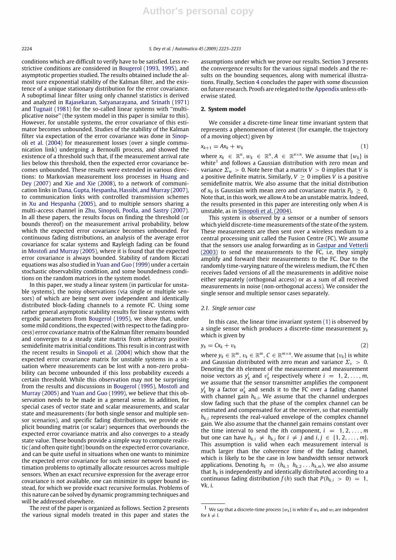
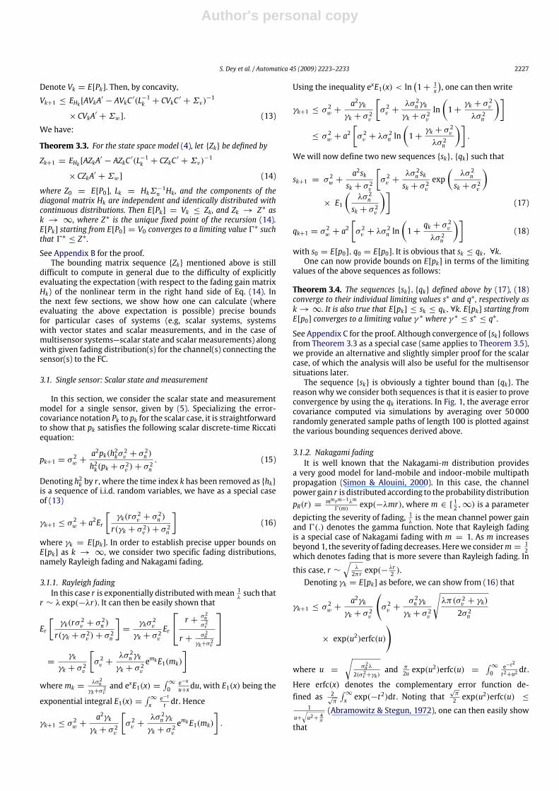
reason why we consider both sequences is that it is easier to proveconvergence by using the qk iterations. In Fig. 1, the average errorcovariance computed via simulations by averaging over 50000randomly generated sample paths of length 100 is plotted againstthe various bounding sequences derived above.

3.1.2. Nakagami fadingIt is well known that the Nakagami-m distribution provides

a very good model for land-mobile and indoor-mobile multipathpropagation (Simon & Alouini, 2000). In this case, the channelpower gain r is distributed according to the probability distributionpR(r) = mmrm−1λm

0(m) exp(−λmr), where m ∈ [ 12 ,∞) is a parameterdepicting the severity of fading, 1

λis the mean channel power gain

and 0(.) denotes the gamma function. Note that Rayleigh fadingis a special case of Nakagami fading with m = 1. As m increasesbeyond 1, the severity of fading decreases. Herewe considerm = 1

2which denotes fading that is more severe than Rayleigh fading. In

this case, r ∼√

λ2πr exp(−

λr2 ).

Denoting γk = E[pk] as before, we can show from (16) that

γk+1 ≤ σ2w +

a2γkγk + σ 2v

(σ 2v +

σ 2n γk

γk + σ 2v

√λπ(σ 2v + γk)

2σ 2n

× exp(u2)erfc(u)

)

where u =√

σ 2n λ

2(σ 2v+γk)and π

2u exp(u2)erfc(u) =

∫∞

0e−t2

t2+u2dt .

Here erfc(x) denotes the complementary error function de-fined as 2

√π

∫∞

x exp(−t2)dt . Noting that

√π

2 exp(u2)erfc(u) ≤

1

u+√u2+ 4π

(Abramowitz & Stegun, 1972), one can then easily show

that

Author's personal copy

2228 S. Dey et al. / Automatica 45 (2009) 2223–2233

0 20 40 60 80 100250

300

350

400

450

500

550

600

time index (k)

aver

age

erro

r co

varia

nce

and

boun

ds

γk

sk

qk

0 20 40 60 80 100400

600

800

1000

1200

1400

1600

1800

time index (k)

aver

age

erro

r co

varia

nce

and

boun

ds

γk

sk

qk

(a) σv = 2.0. (b) σv = 20.0.

Fig. 1. Average error covariance and bounds for Rayleigh fading with various σv values, with a = 1.25, c = 1.0, σw = 1.0, σn = 2.0, λ = 100.

γk+1 ≤ σ2w +

a2γkγk + σ 2v

σ 2v + σn√2λγk√

γk + σ 2v

1

u+√u2 + 4

π

.We can now define two sequences sk, qk as follows:

sk+1 = σ 2w +a2sksk + σ 2v

(σ 2v +

σ 2n sksk + σ 2v

√λπ(σ 2v + sk)2σ 2n

× exp(u2)erfc

(u) )

(19)

qk+1 = σ 2w + a2

σ 2v + σn√2λqk√

σ 2n λ2 +

√σ 2n λ2 +

4π(qk + σ 2v )

(20)

with s0 = E[p0], q0 = E[p0], and u =√

σ 2n λ

2(σ 2v+sk). We can then

similarly have the following theorem which states:

Theorem 3.5. For the case of Nakagami( 12 ) fading, the sequencessk, qk defined above by (19), (20) converge to their individuallimiting values s∗ and q∗, respectively as k → ∞. It is also true thatE[pk] ≤ sk ≤ qk, ∀k. E[pk] starting fromE[p0] converges to a limitingvalue γ ∗ where γ ∗ ≤ s∗ ≤ q∗.

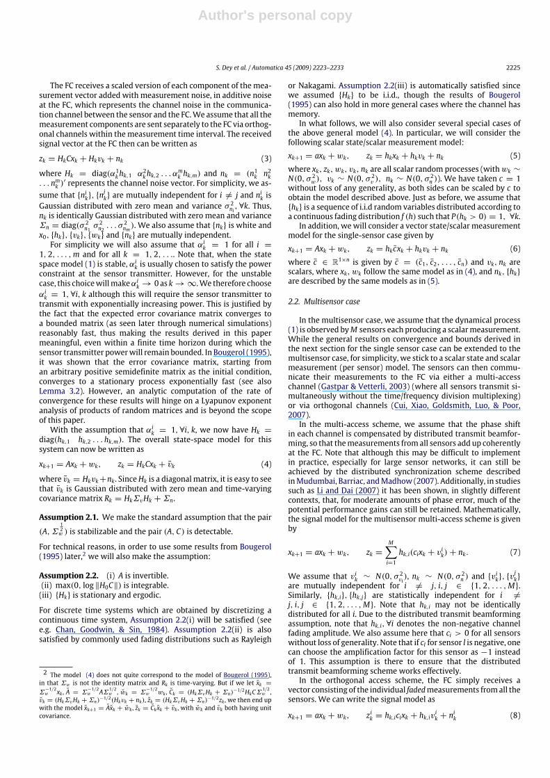
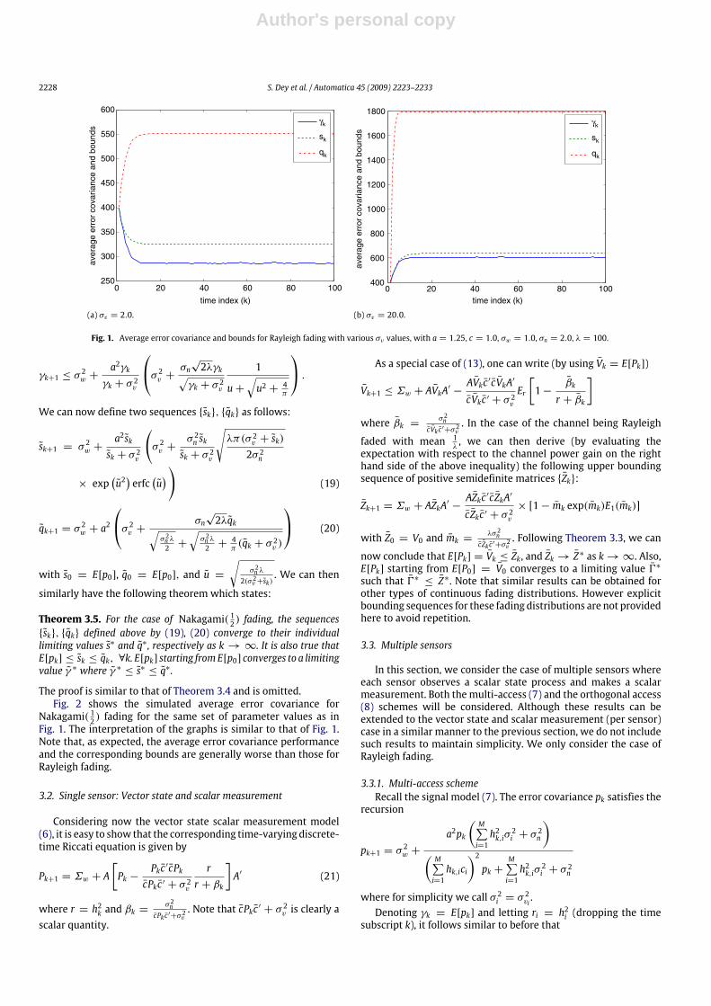
The proof is similar to that of Theorem 3.4 and is omitted.Fig. 2 shows the simulated average error covariance for

Nakagami( 12 ) fading for the same set of parameter values as inFig. 1. The interpretation of the graphs is similar to that of Fig. 1.Note that, as expected, the average error covariance performanceand the corresponding bounds are generally worse than those forRayleigh fading.

3.2. Single sensor: Vector state and scalar measurement

Considering now the vector state scalar measurement model(6), it is easy to show that the corresponding time-varying discrete-time Riccati equation is given by

Pk+1 = Σw + A[Pk −

Pkc ′cPkcPkc ′ + σ 2v

rr + βk

]A′ (21)

where r = h2k and βk =σ 2n

cPk c′+σ 2v. Note that cPkc ′ + σ 2v is clearly a

scalar quantity.

As a special case of (13), one can write (by using Vk = E[Pk])

Vk+1 ≤ Σw + AVkA′ −AVkc ′cVkA′

cVkc ′ + σ 2vEr

[1−

βk

r + βk

]where βk =

σ 2ncVk c′+σ 2v

. In the case of the channel being Rayleigh

faded with mean 1λ, we can then derive (by evaluating the

expectation with respect to the channel power gain on the righthand side of the above inequality) the following upper boundingsequence of positive semidefinite matrices Zk:

Zk+1 = Σw + AZkA′ −AZkc ′cZkA′

cZkc ′ + σ 2v× [1− mk exp(mk)E1(mk)]

with Z0 = V0 and mk =λσ 2n

cZk c′+σ 2v. Following Theorem 3.3, we can

now conclude that E[Pk] = Vk ≤ Zk, and Zk → Z∗ as k→∞. Also,E[Pk] starting from E[P0] = V0 converges to a limiting value 0∗such that 0∗ ≤ Z∗. Note that similar results can be obtained forother types of continuous fading distributions. However explicitbounding sequences for these fading distributions are not providedhere to avoid repetition.

3.3. Multiple sensors

In this section, we consider the case of multiple sensors whereeach sensor observes a scalar state process and makes a scalarmeasurement. Both themulti-access (7) and the orthogonal access(8) schemes will be considered. Although these results can beextended to the vector state and scalar measurement (per sensor)case in a similar manner to the previous section, we do not includesuch results to maintain simplicity. We only consider the case ofRayleigh fading.

3.3.1. Multi-access schemeRecall the signal model (7). The error covariance pk satisfies the

recursion

pk+1 = σ 2w +a2pk

(M∑i=1h2k,iσ

2i + σ

2n

)(M∑i=1hk,ici

)2pk +

M∑i=1h2k,iσ

2i + σ

2n

where for simplicity we call σ 2i = σ2vi.

Denoting γk = E[pk] and letting ri = h2i (dropping the timesubscript k), it follows similar to before that

Author's personal copy

S. Dey et al. / Automatica 45 (2009) 2223–2233 2229

0 20 40 60 80 100350

400

450

500

550

600

time index (k)

aver

age

erro

r co

varia

nce

and

boun

ds

γk

sk

qk

0 20 40 60 80 100400

600

800

1000

1200

1400

1600

1800

time index (k)

aver

age

erro

r co

varia

nce

and

boun

ds

γk

sk

qk

(a) σv = 2.0. (b) σv = 20.0.

Fig. 2. Average error covariance and bounds for Nakagami( 12 ) fading with various σv values, with a = 1.25, c = 1.0, σw = 1.0, σn = 2.0, λ = 100.

γk+1 ≤ σ2w + Er

a2γk

(M∑i=1riσ 2i + σ

2n

)(M∑i=1

√rici

)2γk +

M∑i=1riσ 2i + σ 2n

≤ σ 2w + Er

a2γk

(M∑i=1riσ 2i + σ

2n

)M∑i=1ric2i γk +

M∑i=1riσ 2i + σ 2n

where r = (r1, . . . , rM), and the second inequality follows sincethe ci’s are assumed to be positive. Since we are dealing withRayleigh fading, ri ∼ λi exp(λiri).Now assume the sensors are ordered in descending order of

measurement quality such that

c21σ 21≥c22σ 22≥ · · · ≥

c2Mσ 2M. (22)

We have

Er

M∑i=1riσ 2i + σ

2n

M∑i=1ric2i γk +

M∑i=1riσ 2i + σ 2n

=

σ 21

c21γk + σ21Er2,...,rM

[1+ (A1 −B1)eB1E1(B1)

]where

A1 =λ1

σ 21

(M∑i=2

riσ 2i + σ2n

)and

B1 =λ1

c21γk + σ21

(M∑i=2

ri(c2i γk + σ2i )+ σ

2n

).

By assumption (22),A1 −B1 ≥ 0. Using the inequality exE1(x) <ln(1+ 1

x )would result in very complicated expressions which aredifficult to work with forM > 2. For a simpler expression, we willinstead use the looser inequality exE1(x) < 1

x . Then

Er

M∑i=1riσ 2i + σ

2n

M∑i=1ric2i γk +

M∑i=1riσ 2i + σ 2n

≤σ 21

c21γk + σ21Er2,...,rM

[1+

A1 −B1

B1

]=

σ 21

c21γk + σ21Er2,...,rM

[A1

B1

]

= Er2,...,rM

M∑i=2riσ 2i + σ

2n

M∑2=1ri(c2i γk + σ

2i )+ σ

2n

=

σ 22

c22γk + σ22Er3,...,rM

[1+ (A2 −B2)eB2E1(B2)

]where

A2 =λ2

σ 22

(M∑i=3

riσ 2i + σ2n

)and

B2 =λ2

c22γk + σ22

(M∑i=3

ri(c2i γk + σ2i )+ σ

2n

).

By assumption (22), we also have A2 − B2 ≥ 0. Continuing thisprocess, we eventually arrive at

Er

M∑i=1riσ 2i + σ

2n

M∑i=1ric2i γk +

M∑i=1riσ 2i + σ 2n

≤ σ 2M

c2Mγk + σ2M

×[1+ (AM −BM)eBM E1(BM)

]whereAM =

λMσ 2Mσ 2n ,BM =

λMc2Mγk+σ

2Mσ 2n . Hence

γk+1 ≤ σ2w +

a2γkσ 2Mc2Mγk + σ

2M

[1+ (AM −BM)eBM E1(BM)

].

We can define the bounding sequence

sk+1 = σ 2w +a2skσ 2Mc2Msk + σ

2M

[1+ (AM − BM)eBM E1(BM)

]with AM =

λMσ 2Mσ 2n , BM =

λMc2M sk+σ

2Mσ 2n , and convergence properties

of this sequence can be proved similar to Theorem 3.4. Recallingthe ordering (22), we thus see that we are bounded by the resultassuming just the ‘‘worst’’ sensor in terms of the sensor SNR c2i /σ

2i .

Author's personal copy

2230 S. Dey et al. / Automatica 45 (2009) 2223–2233

0 20 40 60 80 10030

35

40

45

50

55

60

65

70

75

80

time index (k)

aver

age

erro

r co

varia

nce

and

boun

ds

γk

sk

tk

0 20 40 60 80 1000

100

200

300

400

500

600

700

time index (k)

aver

age

erro

r co

varia

nce

and

boun

ds

γk

sk

tk

(a) λ1 = 100, λ2 = 20. (b) λ1 = 100, λ2 = 200.

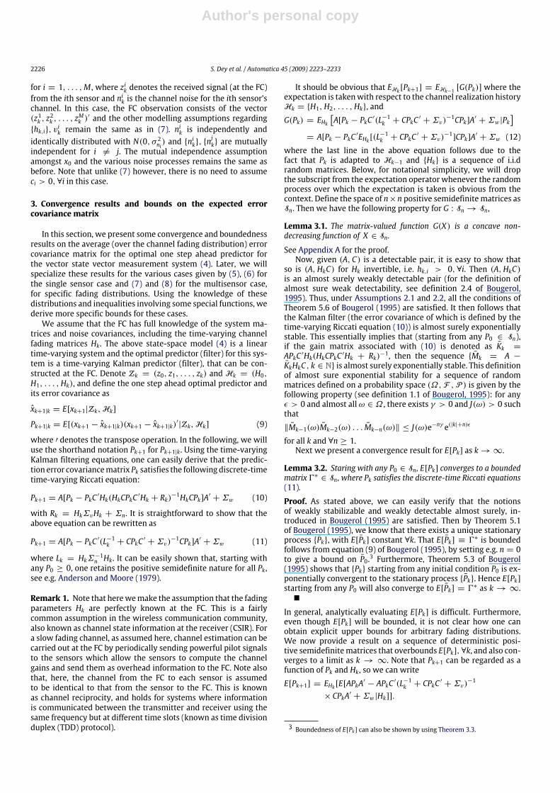
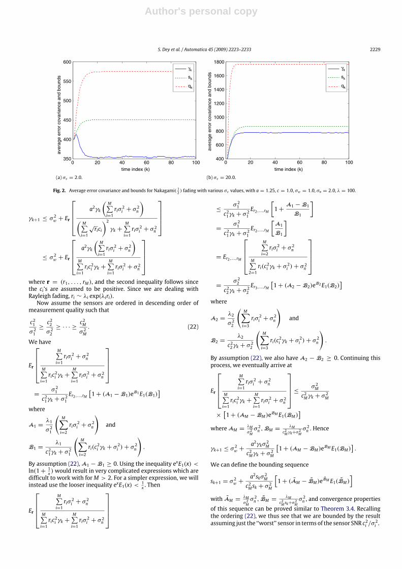
Fig. 3. Average error covariance and bounds for multi-access scheme, with a = 1.25, c1 = 1.0, c2 = 1.0, σw = 1.0, σ1 = 1.0, σ2 = 2.0, σn = 2.0.

An alternative boundConsider the following inequality for xi ≥ 0,

1M∑i=1xi

≤1M2

M∑i=1

1xi

(23)

which is a consequence of the well-known result that the arith-metic mean is greater than or equal to the harmonic mean. Wewill use this inequality to derive an alternative bound. A more at-tractive feature of this bound is that the parameters for all of thesensors will appear in the expressions obtained. Applying the in-equality (23), we have

Er

M∑i=1riσ 2i + σ

2n

M∑i=1ri(c2i γk + σ

2i )+ σ

2n

= Er

M∑i=1riσ 2i + σ

2n

M∑i=1(ri(c2i γk + σ

2i )+

σ 2nM )

≤1M2Er

M∑i=1

M∑j=1rjσ 2j + σ

2n

ri(c2i γk + σ2i )+

σ 2nM

.We can evaluate

Er

M∑j=1rjσ 2j + σ

2n

ri(c2i γk + σ2i )+

σ 2nM

= Eririσ 2i +

∑j6=i

σ 2jλj+ σ 2n

ri(c2i γk + σ2i )+

σ 2nM

=

σ 2i

c2i γk + σ2i[1+ (Ci −Di)eDiE1(Di)] (24)

with Ci =λiσ 2i

(∑j6=i

σ 2jλj+ σ 2n

),Di =

λiσ2n

M(c2i γk+σ2i ). Hence an alter-

native bounding sequence is

tk+1 = σ 2w +a2tkM2

M∑i=1

σ 2i

c2i tk + σ2i

[1+ (Ci − Di)eDiE1(Di)

]where Ci =

λiσ 2i

(∑j6=i

σ 2jλj+ σ 2n

), Di =

λiσ2n

M(c2i tk+σ2i ).

3.3.2. Orthogonal access schemeRecalling the orthogonal accessmodel (8), it can be shownusing

the matrix inversion lemma that the error covariance satisfies

pk+1 = σ 2w +a2pk

1+ pkM∑i=1

h2k,ic2i

h2k,iσ2i +σ

2n

.

Letting γk = E[pk], ri = h2i , we have

γk+1 ≤ σ2w + Er

a2γk

1+ γkM∑i=1

ric2iriσ 2i +σ

2n

.We can compute

Er

1

1+ γkM∑i=1

ric2iriσ 2i +σ

2n

= Er

r1σ 21 + σ2n

(r1σ 21 + σ 2n )(1+ γk

M∑i=2

ric2iriσ 2i +σ

2n

)+ r1c21γk

=

σ 21

σ 21

(1+ γk

M∑i=2

ric2iriσ 2i +σ

2n

)+ c21γk

× Er2,...,rM[1+ (A1 −B1)eB1E1(B1)

]where

A1 =λ1σ

2n

σ 21, B1 =

λ1σ2n

(1+ γk

M∑i=2

ric2iriσ 2i +σ

2n

)σ 21

(1+ γk

M∑i=2

ric2iriσ 2i +σ

2n

)+ c21γk

.

We note that here

A1 −B1 =λ1σ

2n c21γk

σ 21

[σ 21

(1+ γk

M∑i=2

ric2iriσ 2i +σ

2n

)+ c21γk

]

Author's personal copy

S. Dey et al. / Automatica 45 (2009) 2223–2233 2231

is always positive, unlike the multi-access scheme where weneeded the extra assumption (22). Again using the inequalityexE1(x) < 1

x , we obtain

Er

1

1+ γkM∑i=1

ric2iriσ 2i +σ

2n

≤ Er2,...,rM 1

1+ γkM∑i=2

ric2iriσ 2i +σ

2n

≤ · · · ≤

σ 2M

c2Mγk + σ2M[1+ (AM −BM)eBM E1(BM)]

where AM =λMσ

2n

σ 2M,BM =

λMσ2n

σ 2M+c2Mγk. Note, however, that since no

ordering of the sensors is assumed, we could have taken the expec-tations over (r1, . . . , rM) in any order. Hence we have

γk+1 ≤ σ2w + min

i=1,...,M

a2γkσ 2ic2i γk + σ

2i

[1+ (A′i −B ′i )e

B′i E1(B ′i )]

where A′i =λiσ

2n

σ 2i,B ′i =

λiσ2n

σ 2i +c2i γk. We can thus define an upper

bounding sequence

sk+1 = σ 2w + mini=1,...,M

a2skσ 2ic2i sk + σ

2i

[1+ (Ai − Bi)eBiE1(Bi)

]with Ai =

λiσ2n

σ 2i, Bi =

λiσ2n

σ 2i +c2i sk. Convergence properties of the se-

quence can be proved similar to before.An alternative boundSimilar to the multi-access case, we can derive an alternative

bound, again using the inequality (23). For the orthogonal scheme,we get

Er

1

1+ γkM∑i=1

ric2iriσ 2i +σ

2n

= Er 1M∑i=1( 1M +

γkric2iriσ 2i +σ

2n)

≤1M2Er

M∑i=1

11M +

γkric2iriσ 2i +σ

2n

=1M2

M∑i=1

Mσ 2iMc2i γk + σ

2i[1+ (Ci −Di)eDiE1(Di)] (25)

where Ci =λiσ

2n

σ 2i,Di =

λiσ2n

Mc2i γk+σ2i. Thus an alternative bounding

sequence is

tk+1 = σ 2w +a2tkM2

M∑i=1

Mσ 2i[1+ (Ci − Di)eDiE1(Di)

]Mc2i tk + σ

2i

(26)

where Ci =λiσ

2n

σ 2i, Di =

λiσ2n

Mc2i tk+σ2i.

Note also that the expectation in the second line of (25) canbe evaluated without requiring the independence of the channelfading between sensors, so even for spatially correlated channelgains the bound (26) is still valid.

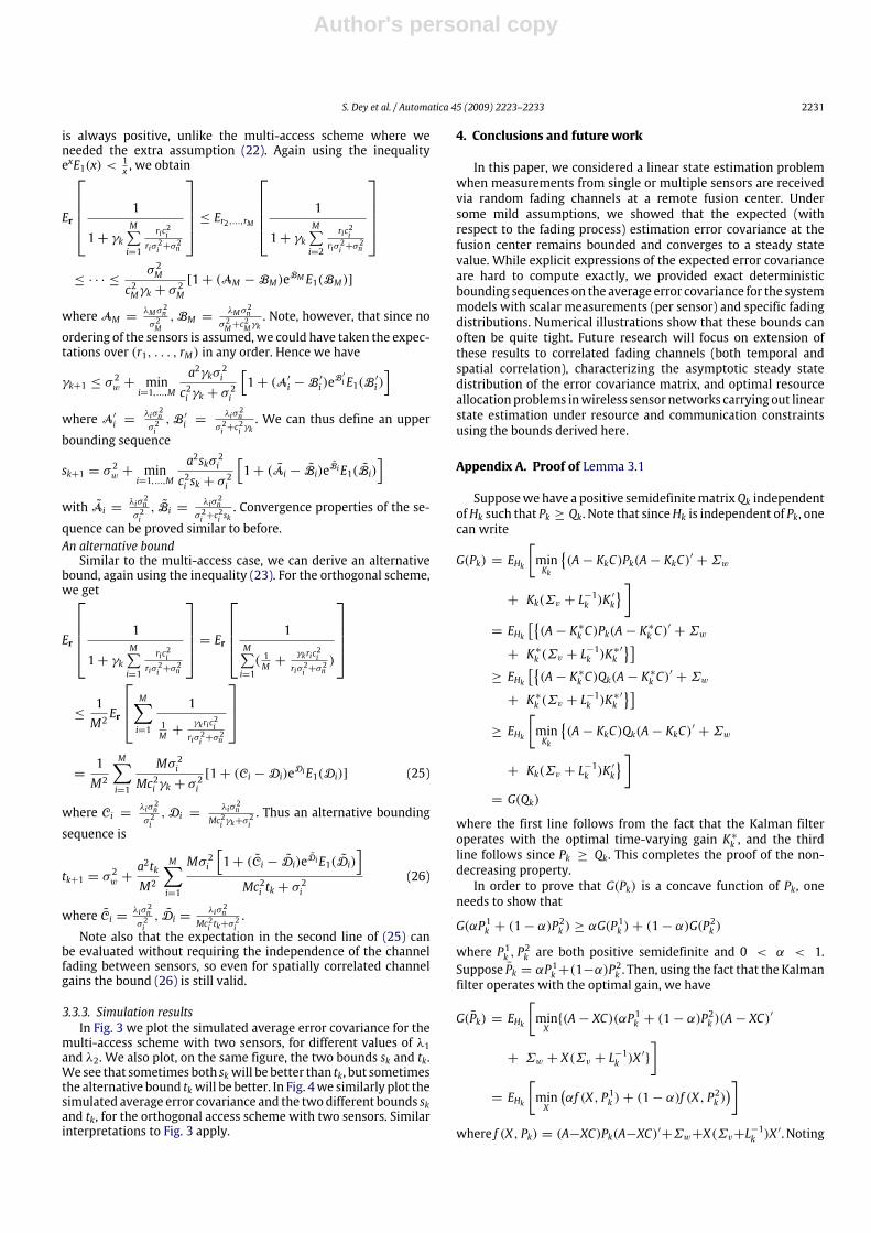
3.3.3. Simulation resultsIn Fig. 3 we plot the simulated average error covariance for the

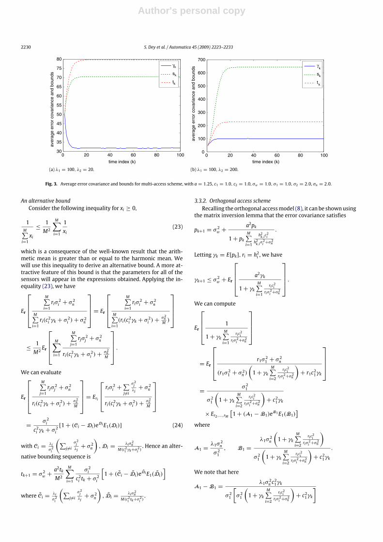
multi-access scheme with two sensors, for different values of λ1and λ2. We also plot, on the same figure, the two bounds sk and tk.We see that sometimes both skwill be better than tk, but sometimesthe alternative bound tkwill be better. In Fig. 4we similarly plot thesimulated average error covariance and the twodifferent bounds skand tk, for the orthogonal access scheme with two sensors. Similarinterpretations to Fig. 3 apply.

4. Conclusions and future work

In this paper, we considered a linear state estimation problemwhen measurements from single or multiple sensors are receivedvia random fading channels at a remote fusion center. Undersome mild assumptions, we showed that the expected (withrespect to the fading process) estimation error covariance at thefusion center remains bounded and converges to a steady statevalue. While explicit expressions of the expected error covarianceare hard to compute exactly, we provided exact deterministicbounding sequences on the average error covariance for the systemmodels with scalar measurements (per sensor) and specific fadingdistributions. Numerical illustrations show that these bounds canoften be quite tight. Future research will focus on extension ofthese results to correlated fading channels (both temporal andspatial correlation), characterizing the asymptotic steady statedistribution of the error covariance matrix, and optimal resourceallocationproblems inwireless sensor networks carrying out linearstate estimation under resource and communication constraintsusing the bounds derived here.

Appendix A. Proof of Lemma 3.1

Supposewehave a positive semidefinitematrixQk independentofHk such that Pk ≥ Qk. Note that sinceHk is independent of Pk, onecan write

G(Pk) = EHk

[minKk

(A− KkC)Pk(A− KkC)′ +Σw

+ Kk(Σv + L−1k )K′

k

]= EHk

[(A− K ∗k C)Pk(A− K

∗

k C)′+Σw

+ K ∗k (Σv + L−1k )K

∗

k′]

≥ EHk[(A− K ∗k C)Qk(A− K

∗

k C)′+Σw

+ K ∗k (Σv + L−1k )K

∗

k′]

≥ EHk

[minKk

(A− KkC)Qk(A− KkC)′ +Σw

+ Kk(Σv + L−1k )K′

k

]= G(Qk)

where the first line follows from the fact that the Kalman filteroperates with the optimal time-varying gain K ∗k , and the thirdline follows since Pk ≥ Qk. This completes the proof of the non-decreasing property.In order to prove that G(Pk) is a concave function of Pk, one

needs to show that

G(αP1k + (1− α)P2k ) ≥ αG(P

1k )+ (1− α)G(P

2k )

where P1k , P2k are both positive semidefinite and 0 < α < 1.

Suppose Pk = αP1k+(1−α)P2k . Then, using the fact that the Kalman

filter operates with the optimal gain, we have

G(Pk) = EHk

[minX(A− XC)(αP1k + (1− α)P

2k )(A− XC)

′

+ Σw + X(Σv + L−1k )X′

]= EHk

[minX

(αf (X, P1k )+ (1− α)f (X, P

2k ))]

where f (X, Pk) = (A−XC)Pk(A−XC)′+Σw+X(Σv+L−1k )X′. Noting

Author's personal copy

2232 S. Dey et al. / Automatica 45 (2009) 2223–2233

0 20 40 60 80 10045

50

55

60

65

70

75

time index (k)

aver

age

erro

r co

varia

nce

and

boun

ds

γk

sk

tk

0 20 40 60 80 10050

100

150

200

250

300

350

time index (k)

aver

age

erro

r co

varia

nce

and

boun

ds

γk

sk

tk

(a) λ1 = 100, λ2 = 20. (b) λ1 = 100, λ2 = 200.

Fig. 4. Average error covariance and bounds for orthogonal scheme, with a = 1.25, c1 = 1.0, c2 = 1.0, σw = 1.0, σ1 = 1.0, σ2 = 2.0, σn = 2.0.

that f (X, Pk) is an affine function in Pk, and pointwise minimum ofan affine function is a concave function, it is clear that

G(Pk) ≥ Ehk

[αmin

Xf (X, P1k )+ (1− α)minX

f (X, P2k )]

= αG(P1k )+ (1− α)G(P2k )

which completes the proof of concavity.

Appendix B. Proof of Theorem 3.3

The fact that Vk ≤ Zk follows from the non-decreasing propertyof Lemma 3.1 and induction.Let us call

fH(X) = AXA′ − AXC ′(L−1 + CXC ′ +Σv)−1CXA′ +Σw

where L = HΣ−1n H . First we show that there exists a fixed pointZ∗ that satisfies

Z∗ = EH [fH(Z∗)].

The function fH(X) has the following properties:

(1) H1 ≤ H2 ⇒ fH1(X) ≥ fH2(X)4

(2) X ≤ Y ⇒ fH(X) ≤ fH(Y ).

Property (1) canbe easily shownbyusingCorollary 7.7.4 (a) ofHornand Johnson (1985) and Property (2) is well-known.Define T : Sn → Sn by

T (X) = EH [fH(X)].

Then by Theorem 7.A of Zeidler (1986), a fixed point (i.e. a solutionto the equation T (X) = X) will exist if the following five conditionshold:

(i) T is monotone increasing, i.e. X ≤ Y ⇒ T (X) ≤ T (Y ),(ii) T is a compact operator,(iii) Sn is a normal order cone, i.e. ∃c > 0 and some norm ‖·‖ such

that 0 ≤ X ≤ Y ⇒ ‖X‖ ≤ c‖Y‖,∀X, Y ∈ Sn,(iv) ∃uwith u ≤ Tu,(v) ∃v with v ≥ Tv.

4 For diagonal matrices, H1 ≤ H2 is equivalent to all the diagonal entries of H1being less than or equal to the corresponding diagonal entries of H2 .

Condition (i) follows from property (2) of the function fH(X). Forcondition (ii), since Sn is a subset of a finite dimensional space,T is continuous, and the semi-definite cone Sn is a closed set,compactness of T follows by example 2.10 of Zeidler (1986). Forcondition (iii), note that X ≤ Y implies λmax(X) ≤ λmax(Y ), whereλmax(X) is the largest (positive) eigenvalue of X . Since X and Y aresymmetric, the singular values are the same as the eigenvalues,hence ‖X‖ ≤ ‖Y‖ in the spectral norm, and the condition for Snto be a normal order cone is satisfied for c = 1. For condition (iv),u = 0 suffices, since T (0) = EH [fH(0)] = Σw ≥ 0. It remainsto show condition (v). Now for any invertible H , one can alwaysfind an X such that fH(X) < X , by using e.g. the construction in theproof of Theorem 1 of Bitmead, Gevers, Petersen, and Kaye (1985).Let H∗ = diag(h∗, . . . , h∗), and let X∗ (dependent on H∗) satisfyfH∗(X∗) < X∗. Let us write

EH [fH(X∗)] = EH [fH(X∗)|H ≥ H∗]P(H ≥ H∗)+ EH [fH(X∗)|H 6≥ H∗]P(H 6≥ H∗).

Then we have EH [fH(X∗)|H ≥ H∗] < X∗ by property (1), andP(H ≥ H∗) → 1 as h∗ → 0. We also have that the matrixEH [fH(X∗)|H 6≥ H∗] is bounded above by Σw + AX∗A, and P(H 6≥H∗) → 0 as h∗ → 0. Hence for sufficiently small h∗, there existsan X∗ such that EH [fH(X∗)] ≤ X∗, and condition (v) is satisfied byletting v be this X∗. Thus all the conditions for the existence of afixed point Z∗ such that Z∗ = EH [fH(Z∗)] are satisfied.Finally, we show convergence of Zk to Z∗ starting from arbi-

trary initial conditions, thus proving uniqueness of the fixed pointZ∗. We will use Theorem 3.3 of Krasnosel’skii, Vainikko, Zabreiko,Rutitskii, and Stetsenko (1972) (see also Theorem 46.1 of Kras-nosel’skiı & Zabreıko, 1984), which gives conditions for a fixedpoint to be unique, provided one actually exists. We need to showthat T is ‘‘u0-concave’’, i.e. there is some u0 ∈ Sn such that:

(i) For any nonzero X ∈ Sn, ∃α(X) > 0, β(X) > 0 such that

αu0 ≤ TX ≤ βu0.

(ii) For each X such that αu0 ≤ X ≤ βu0, and each t ∈ (0, 1),∃η(X, t) > 0 such that

T (tX) ≥ (1+ η)tT (X).

Under the assumption that Σw > 0, we can easily verify thattaking u0 = I will satisfy these conditions. Since we havepreviously shown that there does exist a fixed point Z∗, Theorem3.3 of Krasnosel’skii et al. (1972) then shows that Zk converges toZ∗ for arbitrary Z0 ∈ Sn.

Author's personal copy

S. Dey et al. / Automatica 45 (2009) 2223–2233 2233

Appendix C. Proof of Theorem 3.4

Consider the Eqs. (17) and (18). Note that the right hand sidesof (17) and (18) are increasing functions of sk and qk respectively,which implies that both sk and qk are monotonic sequences.Given that γ0 = E[p0] = s0 = q0, it clearly follows that γ1 ≤s1 ≤ q1. Using the increasing property mentioned above, one canthen prove by induction that γk ≤ sk ≤ qk, ∀k = 1, 2, . . .. Weknow that as a special case of Lemma 3.2, γk = E[pk] converges toa limit (say γ ∗) as k→∞.We now show that qk also converges to a limit (denoted by q∗)

as k → ∞. In order to prove this, we rewrite (18) as qk+1 =l(qk), where l(qk) represents the right hand side of (18). It isstraightforward to show that the mapping q = l(q) has a uniquefixed point. However, in order to prove the convergence of therecursion qk+1 = l(qk) we use the standard function propertiesof the function l(q) (Yates, 1995), namely positivity, monotonicity(these two are obvious) and scalability. In order to show scalability,wehave to show thatβl(q) > l(βq) forβ > 1. This follows because

ln(1+

βqk + σ 2vλσ 2n

)< ln

(1+

β(qk + σ 2v )λσ 2n

)< β ln

(1+

qk + σ 2vλσ 2n

)where the first inequality follows since β > 1 and the secondinequality follows since ln(1+βx) < β ln(1+x) for x > 0, β > 1.Since l(q) is a standard function, the recursion qk+1 = l(qk) willconverge to the unique fixed point q∗.Now sk is a monotonic sequence sandwiched between two

convergent sequences qk and γk (the limits of the two se-quences are in general different). Hence sk can be bounded fromboth above and below, so converges to a limit s∗. Since γk ≤ sk ≤qk, ∀k = 1, 2, . . ., we have γ ∗ ≤ s∗ ≤ q∗.

References

Abramowitz, M., & Stegun, I. A. (1972). Handbook of mathematical functions. NewYork: Dover Publications Inc.

Anderson, B. D. O., & Moore, J. B. (1979). Optimal filtering. New Jersey: Prentice Hall.Anderson, B. D. O., & Moore, J. B. (1981). Detectability and stabilizability of time-varying discrete-time linear systems. SIAM Journal on Control and Optimization,19(1), 20–32.

Bitmead, R. R., Gevers, M. R., Petersen, I. R., & Kaye, R. J. (1985). Monotonicityand stabilizability properties of solutions of the Riccati difference equation:Propositions, lemmas, theorems, fallacious conjectures and counterexamples.Systems and Control Letters, 5(5), 309–315.

Bougerol, P. (1993). Kalman filtering with random coefficients and contractions.SIAM Journal on Control and Optimization, 31(4), 942–959.

Bougerol, P. (1995). Almost sure stabilizability and Riccati’s equation of linearsystems with random parameters. SIAM Journal on Control and Optimization,33(3), 702–717.

Chan, S. W., Goodwin, G. C., & Sin, K. S. (1984). Convergence properties of theRiccati difference equation in optimal filtering of nonstabilizable systems. IEEETransactions on Automatic Control, 29(2), 110–118.

Cui, S., Xiao, J.-J., Goldsmith, A., Luo, Z.-Q., & Poor, H. V. (2007). Estimationdiversity and energy efficiency in distributed sensing. IEEE Transactions on SignalProcessing , 55(9), 4683–4695.

Dana, A. F., Gupta, V., Hespanha, J. P., Hassibi, B., & Murray, R. M. (2007). Estimationover communication networks: Performance bounds and achievability results.In Proc. American control conf. (pp. 3450–3455).

Gastpar, M., & Vetterli, M. (2003). Source-channel communication in sensornetworks. Springer Lecture Notes in Computer Science, 2634, 162–177.

Horn, R. A., & Johnson, C. R. (1985). Matrix analysis. Cambridge, United Kingdom:Cambridge University Press.

Huang, M., & Dey, S. (2007). Stability of Kalman filtering with Markovian packetlosses. Automatica, 43, 598–607.

Jazwinski, A. H. (1970). Stochastic processes and filtering theory. New York: AcademicPress.

Krasnosel’skii, M. A., Vainikko, G. M., Zabreiko, P. P., Rutitskii, Y. B., & Stetsenko, V.Y. (1972). Approximate solution of operator equations. Groningen, Netherlands:Wolters-Noordhoff Publishing.

Krasnosel’skiı, M. A., & Zabreıko, P. P. (1984). Geometrical methods of nonlinearanalysis. Berlin: Springer-Verlag.

Li, W., & Dai, H. (2007). Distributed detection in wireless sensor networks using amultiple access channel. IEEE Transactions on Signal Processing , 55(3), 822–833.

Mostofi, Y., & Murray, R. M. (2005). On dropping noisy packets in Kalman filteringover a wireless fading channel. Proc. American control conf. (pp. 4596–4600).

Mudumbai, R., Barriac, G., & Madhow, U. (2007). On the feasibility of distributedbeamforming in wireless networks. IEEE Transactions on Wireless Communica-tions, 6(5), 1754–1763.

Rajasekaran, P. K., Satyanarayana, N., & Srinath, M. D. (1971). Optimum linearestimation of stochastic signals in the presence of multiplicative noise. IEEETransactions on Aerospace and Electronic Systems, 7(3), 462–468.

Simon, M., & Alouini, M.-S. (2000). Digital communication over fading channels. NewYork: John Wiley and Sons.

Sinopoli, B., Schenato, L., Franceschetti, M., Poolla, K., Jordan, M. I., & Sastry, S. S.(2004). Kalman filtering with intermittent observations. IEEE Transactions onAutomatic Control, 49(9), 1453–1464.

Tugnait, J. K. (1981). Stability of optimum linear estimators of stochastic signalsin white multiplicative noise. IEEE Transactions on Automatic Control, 26(3),757–761.

Xie, L., & Xie, L. (2008). Stability of a randomRiccati equationwithMarkovian binaryswitching. IEEE Transactions on Automatic Control, 53(7), 1759–1764.

Xu, Y., & Hespanha, J. P. (2005). Estimation under uncontrolled and controlledcommunications in networked control systems. Proc. IEEE conf. decision andcontrol (pp. 842–847).

Yates, R. D. (1995). A framework for uplink power control in cellular radio systems.IEEE Journal on Selected Areas in Communications, 13(7), 1341–1347.

Yuan,W., & Guo, L. (1999). On stability of random Riccati equations. Science in China(Series E), 42(2), 136–148.

Zeidler, E. (1986). Nonlinear functional analysis and its applications I: Fixed-pointtheorems. New York: Springer-Verlag.

Zhu, B., Sinopoli, B., Poolla, K., & Sastry, S. (2007). Estimation over wireless sensornetworks. Proc. American control conf. (pp. 2732–2737).

Subhrakanti Dey was born in Calcutta, India, in 1968.He received the B.Tech. and M.Tech. degrees from theDepartment of Electronics and Electrical CommunicationEngineering, Indian Institute of Technology, Kharagpur,India, in 1991 and 1993, respectively, and the Ph.D.degree from the Department of Systems Engineering,Research School of Information Sciences and Engineering,Australian National University, Canberra, Australia, in1996.He has been with the Department of Electrical and

Electronic Engineering, University ofMelbourne, Parkville,Australia, since February 2000, where he is currently a full Professor. FromSeptember 1995 to September 1997 and September 1998 to February 2000, hewas a postdoctoral Research Fellow with the Department of Systems Engineering,Australian National University. From September 1997 to September 1998, hewas a post-doctoral Research Associate with the Institute for Systems Research,University of Maryland, College Park. His current research interests includenetworked control systems, wireless communications and networks, signalprocessing for sensor networks, and stochastic and adaptive estimation and control.Dr. Dey currently serves on the Editorial Board of the IEEE Transactions on Signal

Processing and Elsevier Systems and Control Letters. Hewas also anAssociate Editorfor the IEEE Transactions on Automatic Control during 2005–2007. He is a SeniorMember of IEEE.

Alex S. Leong was born in Macau in 1980. He receivedthe B.S. degree in mathematics and B.E. degree inElectrical Engineering in 2003, and Ph.D. degree inElectrical Engineering in 2008, all from the University ofMelbourne.He is currently a research fellow in the Department

of Electrical and Electronic Engineering at the Universityof Melbourne. His research interests include statisticalsignal processing, signal processing for sensor networks,and networked control systems.Dr. Leong was the recipient of the L. R. East Medal

(2003) from Engineers Australia and an Australian Postdoctoral Fellowship (2009)from the Australian Research Council.

Jamie S. Evans was born in Newcastle, Australia, in 1970.He received the B.S. degree in Physics and the B.E. degree inComputer Engineering from the University of Newcastle,in 1992 and 1993, respectively, where he received theUniversity Medal upon graduation. He received the M.S.and the Ph.D. degrees from the University of Melbourne,Parkville, Australia, in 1996 and 1998, respectively, both inElectrical Engineering, and was awarded the Chancellor’sPrize for excellence for his Ph.D. thesis. From March1998 to June 1999, he was a Visiting Researcher inthe Department of Electrical Engineering and Computer

Science, University of California, Berkeley. He returned to Australia to take up aposition as Lecturer at theUniversity of Sydney, Australia,where he stayed until July2001. Since that time, he has been with the Department of Electrical and ElectronicEngineering, University of Melbourne, where he is now an Associate Professor andReader. His research interests are in communications theory, information theory,and statistical signal processingwith a focus onwireless communications networks.