Slipping detection and avoidance based on Kalman filter

Alberto Cavallo, Giuseppe De Maria, Ciro Natale∗, Salvatore Pirozzi

Dipartimento di Ingegneria Industriale e dell’Informazione,

Seconda Universita degli Studi di Napoli, 81031 Aversa, Italy

Abstract

The purpose of this paper is to present the latest slipping detection and avoid-

ance algorithms developed by the authors for application in robotic manipu-

lation tasks. Slipping can happen not only in quasi-static conditions such as

in grasping tasks but also during dynamic manipulation, therefore the avail-

ability of slip control techniques effective in both conditions, such as those

proposed here, are essential in real robotic applications. A new algorithm is

also proposed to estimate on-line the actual friction coefficient at the contact

with the manipulated object by means of a preliminary exploration phase,

thus enabling safe manipulation of objects with unknown surface properties.

A detailed dynamic simulator is presented and experimentally validated on

a mechatronic test bench used for proving the effectiveness of the proposed

approach.

Keywords: Robotic manipulation, Slipping detection, Slipping avoidance,

Friction coefficient estimation.

1. Introduction

Many studies proved that manipulation ability is enabled by tactile and

force sensing, especially the ability to sense the contact condition between

∗Corresponding authorEmail address: ciro.natale@unina2.it (Ciro Natale)

Preprint submitted to Mechatronics May 12, 2014

the object and the fingers [1]. A neurophysiological study on human manip-

ulation [2] demonstrated that humans are able to keep objects under load

perturbations in the direction tangential to the contact surface by adjusting

fingertip force vectors so that the force in the direction normal to the contact

surface (the so-called grip force) is high enough in relation to the tangential

component to prevent slippage, but, at the same time, avoiding deformation

of the object. Contact forces and torques vectors at the fingertips, con-

tact point/area locations, orientation of the contact surface, shape and force

distribution of the contact area, friction coefficient are the physical quanti-

ties and parameters that play a key role in this kind of tasks. Among them,

knowledge of the friction coefficient is particularly relevant for a safe grasping

and manipulation [3, 4]. Various solutions for estimation of this parameter

exist in the literature but most of them rely on ad-hoc sensors [5, 6]. All these

algorithms are mainly based on the Coulomb friction law, which is the most

celebrated model exploited for robotic manipulation. However, such model

does not take into account some phenomena taking place during the contact

between two surfaces. Therefore, many more sophisticated friction models,

such as [7, 8, 9], have been proposed and used in motion control systems

for friction compensation [10] and in robotics [11] for object detection and

recognition, or for dynamic modeling of grasping [12]. Among such friction

models, the LuGre model has been selected for reproducing as accurately

as possible in a dynamic simulator the experimentally observed phenomena,

and it will be exploited to tune the control algorithm parameters.

Slip detection plays a central role not only in ensuring a stable grasp by

adjusting the grip force, but also in manipulation and tactile exploration, as

during the slippage, contact forces or more generic tactile sensory data can

provide information about the object properties such as roughness, compli-

2

ance and shape. A recent survey on slipping detection methods is [13], where

a taxonomy of slip sensors is proposed comprising four categories based on

the detected physical quantity associated to slip: displacement, force, heat,

micro-vibration. The slip control proposed in the present paper belongs to

the force sensor category. Nevertheless, the authors of the survey believe that

research efforts are still needed not only in terms of hardware development

but also in terms of efficient computational methods. Many recent papers,

e.g. [14, 15, 16, 17, 18], dealing with slip control demonstrate that research

effort is still needed in terms of both hardware progress and algorithmic

advancements.

If slip detection is certainly a feature of primary importance, slipping

avoidance is definitely the final objective during grasping and manipulation

of an object. Therefore, availability of good detection algorithms is useless

without an effective slip avoidance technique. Methods for slip control can

basically be divided into two categories, techniques that exploit contact force

measurements and techniques that exploit the geometric characteristics of

the contact area. A recent work belonging to the first category is [19], where

a sliding mode control strategy is adopted to control the grip force on the

basis of a binary slip detection signal obtained through an array of linear

filters of the measured shear force. Similarly to other approaches of the same

category, whose references can be found in the cited paper, the grip force

is always increased on the basis of the slip event detection. Even though

these approaches are suitable for grasping tasks and for slip avoidance in

case of unknown or changing friction coefficient, they could not be effective

during manipulation tasks where dynamic interaction forces dominate. In

such cases, the grip force should be adjusted depending on the dynamic

loading conditions and thus the slip control action should be able to increase

3

and also decrease the grip force.

An example of work belonging to the second category and still focusing on

grasping tasks is [20], where a vision-based slip margin feedback is proposed

for slip control. Similarly to other approaches that exploit contact surface

information, complex sensing equipments are needed to obtain a distributed

measurement, simple force sensors are not enough.

This paper extends previous work of the authors on slipping control that

initiated in [17], where the force/tactile sensor developed in [21] was exploited

to estimate the friction coefficient using an off-line technique; then such pa-

rameter was used to setup an elementary slip control algorithm assuming to

work in quasi-static conditions. The same sensor was then used in [15] within

a slip control loop that exploited the residual of an Extended Kalman Filter

(EKF). However, the EKF was not purposefully designed for the slip control

law, but it was mainly devoted to estimate position and orientation of the

object in contact with the hemispherical soft finger tip. In the recent pa-

per [16], the same EKF was exploited to setup a slipping detection technique

and to calculate the orientation of the object in contact with the soft tactile

sensor in the 3D case, so as to allow a correct estimation of the normal and

tangential components of the contact force and thus of the friction coefficient.

With respect to this previous work, the novel contributions of the present

paper mainly consist in a new slipping detection algorithm based on a sim-

ple linear Kalman filter (KF), though it assumes that tangential and normal

components of the contact force are already available, e.g. through the EKF

cited above, that is mandatory for in-hand manipulation. The second con-

tribution is a technique to estimate the friction coefficient by exploiting the

slipping detection algorithm. This technique is applied during a preliminary

exploration phase of the object to manipulate and it can estimate the actual

4

friction coefficient of the contact surface, which depends on environmental

conditions such as humidity, temperature and cleanliness. The third contri-

bution is a slip control law that exploits the KF residual and the estimated

friction coefficient to compute a grip force adjustment. The control strategy

can work not only in static conditions but also when dynamic interaction

forces dominate.

The paper is organized as follows. Section 2 is focused on the dynamic

modelling of the contact between an object and a compliant sensor pad

mounted on a force sensor able to measure both normal and tangential com-

ponents of the contact force. Contact friction is modelled according to the

LuGre dynamic model, which is briefly reviewed and then implemented in

the simulator. Section 3 presents the design of the KF based on the dynamic

model of the previous section, and whose residual is exploited to detect the

slippage and as input to the slipping control algorithm presented later in

Section 5. The filter equations reveal that its residual contains the effects

of forces not balanced by the static friction, including inertial forces, hence

the idea is to exploit the residual as a tool for slip detection and avoidance.

The experimental setup used to carry out the experiments is described in

Section 4, where the model dynamic parameters are tuned so as to have a

good accordance between the simulation and the experimental results. The

experimental validation of the slipping detection method is then presented.

The slipping avoidance algorithm is designed in Section 5 on the basis of the

dynamic model and the developed simulator. The haptic exploration proce-

dure for friction coefficient estimation is also presented in this section as a

method to provide this parameter needed by the slip controller. Both simula-

tion and experimental results, that confirm the effectiveness of the proposed

approach, are presented.

5

xxxxxxxxxxxxxxxxxxxxxxxxxxxxxxxxxxxxxxxxxxxxxxxxxxxxxxxxxxxxxxxxxxxxxxxxxxxxxxxxxxxxxxxxxxxxxxxxxxxxxxxxxxxxxxxxxxxxxxxxxxxxxxxxxxxxxxxxxxxxxxxxxxxxxxxxxxxxxxxxxxxxxxxxxxxxxxxxxxxxxxxxxxxxxxxxxxxxxxxxxxxxxxxxxxxxxxxxxxxxxxxxxxxxxxxxxxxxxxxxxxxxxx

xxxxxxxxxxxxxxxxxxxxxxxxxxxxxxxxxxxxxxxxxxxxxxxxxxxxxxxxxxxxxxxxxxxxxxxxxxxxxxxxxxxxxxxxxxxxxxxxxxxxxxxxxxxxxxxxxxx

xxxxxxxxxxxxxxxxxx

xxxxx

xxxxxxxxx

xxxxx

xxxxxx

xxxxxxx

xxxxxx

xxxxxxxxxxx

xxxxx

xxxxxxxxxxxxxxxxxxxxxxxxxxxxxxxxxxxxxxxxx

m

Mft

fn

kβ

friction force g(x, fn)

x1

x3sensor pad

object

sliding surface

Figure 1: Sketch of the contact model: tangential dynamics.

2. Modelling

The dynamics of the contact between the sensor and the object is mod-

elled taking into account the inertia of both the sensor pad (assumed de-

formable) and the object as well as the friction force at the contact surface.

The aim of the analysis carried out in this section is to describe the dynamics

of the object slippage when both normal and tangential forces are applied to

it, therefore it is sufficient to write the equations of motion only along the

tangential component of the external force, call it ft.

With reference to Fig. 1, let m be the mass of the moving part of the

force sensor (the sensor pad), k its stiffness, β the damping coefficient of the

material andM the mass of the manipulated object. The friction force acting

between the two contact surfaces will be modelled by resorting to the LuGre

model, which is able to describe the complex phenomena that happen during

a friction contact and it is indicated as g(x, fn), where fn is the normal load

and x = ( x1 x2 x3 x4 x5 )T is the state vector of the dynamic model,

defined as follows: x1 and x3 are the displacements of the sensor pad and of

the object, respectively, x2 = x1 and x4 = x3 are their velocities, thus x2−x4

is the relative speed between object and sensor pad. x5 is the state of the

6

dynamic friction model whose meaning will be detailed below.

The equations of motion can be easily written in the form

mx2 + kx1 + βx2 + g(x, fn) = 0 (1)

Mx4 − g(x, fn) = ft (2)

x5 = n(x, fn) (3)

where the expressions of the friction force g(x, fn) and of the nonlinear func-

tion n(x, fn) depend on the specific friction model that one intends to adopt.

In the case of the LuGre friction model [9], they are defined by the following

equations

g(x, fn) = σ0x5 + (σ1 + σ2)(x2 − x4)− σ0σ1|x2 − x4|

s(x, fn)x5 (4)

n(x, fn) = x2 − x4 − σ0|x2 − x4|

s(x, fn)x5, with (5)

s(x, fn) = µdfn + fn(µs − µd)e−(

x2−x4v0

)2

, (6)

where µd ≤ µs is the kinetic friction coefficient, σ0 is the asperity stiffness, σ1

is the micro-viscous friction coefficient, σ2 is the viscous friction coefficient

and v0 is the threshold velocity for the activation of the Stribeck effect. The

meaning of the state variable x5 is the average micro-displacement of the

contact surface asperities.

It can be shown that for fn → ∞ the system becomes linear. In this

case, for every constant value of ft, no relative motion between the object

and the sensor can occur since the relative speed between object and sensor

pad x2 − x4 → 0, because the static gain of the system with ft as input

and x2 − x4 as output is zero. For a time-varying ft, the relative speed is

practically zero since only micro-displacements are allowed (the higher σ0,

the lower the relative speed is). It is well-known that, for finite values of fn,

7

the same happens until ft is below the so-called ‘break-away force’, which,

for a constant ft, is the stiction force µsfn. However, if the rate of the applied

force ft increases, the break-away force decreases, and this phenomenon is

also captured by the LuGre model. It is also well-known, see e.g. [9, 22],

that the break-away force reaches a minimum asymptotic value as the rate

of the applied tangential load increases. This means that, even in dynamic

conditions, there always exists a normal load high enough to keep the relative

velocity to zero.

For the design of the slipping detection strategy presented in the following

section, it is convenient to express the equations of motions in the state space

form

x1(t) = x2(t) (7)

x2(t) = −k

mx1(t)−

β

mx2(t)−

1

mg(x, fn) (8)

x3(t) = x4(t) (9)

x4(t) =1

Mft +

1

Mg(x, fn) (10)

x5(t) = n(x, fn) (11)

The slipping detection technique, proposed in Section 3, is based on the

solution of the state estimation problem for such contact model. Whereas,

the slipping avoidance control algorithm, proposed in Section 5, will exploit

the normal load fn as control input to act on this system to avoid slippage,

i.e., keeping the relative velocity x2 − x4 practically zero with a limited fn.

3. Slipping detection algorithm

The slipping detection algorithm proposed in this paper is based on a state

observer designed for the contact model presented in the previous section.

The state space equations (7)-(11) along with the output equation, which

8

models the elastic force kx1 measured by the sensor, can be written in the

form

x(t) = Fx(t) +w(t) (12)

y(t) = hTx(t) + v(t) (13)

where v(t) denotes the measurement noise and the matrices F , h are defined

as

F =

0 1 0 0 0

0 0 0 0 0

0 0 0 1 0

0 0 0 0 0

0 0 0 0 0

, h =

k

0

0

0

0

, (14)

and the vector w is

w(t) =

0

−k

mx1 −

β

mx2 −

1

mg(x, fn)

01

Mft +

1

Mg(x, fn)

n(x, fn)

. (15)

Note that the linear terms in x1 and x2 have been included in the dis-

turbance in order not to have the dynamic matrix F be dependent on the

knowledge of the dynamic parameters β and m, which are not easy to esti-

mate accurately.

Observing that, under quasi-static conditions, if no macro-slippage oc-

curs between the object and the sensor, i.e., if the relative velocity x2 − x4

is practically zero, then the nonlinear function n(x, fn) = 0, the friction

force g(x, fn) practically balances the external tangential force ft and the

elastic reaction of the sensor, namely g(x, fn) = −ft = −kx1. Under such

9

assumptions it is w = 0. On the other hand, as soon as there is a slipping

event, i.e., a pre-sliding regime builds up, the force balance above no longer

holds and the vector w 6= 0 acts as a disturbance on the linear system with

dynamic matrix F . Therefore, by designing a suitable state observer assum-

ing that the system dynamics is purely linear (w = 0), it is expected that

as soon as the disturbance vector becomes non null, the estimation error of

the observer increases, thus revealing a pre-sliding condition. By inspect-

ing equations (12)-(13), it is straightforward to notice that the system with

w = 0 is already in the Kalman canonical form and that it is not completely

observable with an observable dynamics described by the equations

z(t) = F oz(t) (16)

y(t) = hTo z(t) (17)

where z = ( x1 x2 )T and the matrices F o and ho are

F o =

0 1

0 0

, ho =

k

0

.

Note that the states x3, x4 and x5 are not observable from y, and for this

reason will no longer be used in the sequel. The first step of the detection

algorithm is the design of a state estimator and this will be done by resorting

to the discrete-time KF, by firstly writing the discrete-time version of the

dynamic system (16)-(17) using the Euler method. Denote with h ∈ Z the

discrete-time variable related to the continuous time by th = hT , being T the

sampling time and with zh = z(th), yh = y(th), vh = v(th) all the variables

sampled at the hth time instant. The equations of the system whose state

has to be estimated are

zh+1 = F ozh +wh (18)

yh = hTo zh + vh (19)

10

where, with a slight abuse of notation, the dynamic matrix and the distur-

bance wh = w(th) are

F o =

1 T

0 1

, wh =

0

−k

mz1h −

β

mz2h −

1

mg(x, fn)

(20)

and the measurement noise vh is assumed a Gaussian white process with

covariance V > 0, uncorrelated with hTo zh. If also the state disturbance wh

were a Gaussian white noise uncorrelated with zh with covariance matrix

W ≥ 0 (and this is the case if no slip occurs because wh = 0), then the mean

of the state estimation error of a standard linear KF for the system (18)-(19)

would be zero. Whereas, it is expected that the error starts increasing as

soon as wh 6= 0, i.e., when a slip occurs, since it actually is strictly correlated

with the system state. In fact, it is a function of the state itself, and thus its

presence is able to bias the state estimate. This is the idea at the basis of

the slipping detection algorithm, which simply monitors the residual of the

following KF

zh+1|h = F ozh|h (21)

P h+1|h = F oP h|hFTo +W (22)

Kh = P h+1|hhTo

(

hTo P h+1|hho + V

)−1

(23)

yh+1|h = hTo zh+1|h (24)

eh+1 = yh+1 − yh+1|h (25)

zh+1|h+1 = zh+1|h +Kheh+1 (26)

P h+1|h+1 = (I −KhhTo )P h+1|h (27)

yh+1|h+1 = hTo zh+1|h+1 (28)

with initial conditions z0|0 = 0, P 0|0 = W , where zh|h and P h|h denote the

estimate of the mean and covariance of the system state at the hth time

11

instant given the observations up to h. The error eh is expected to increase

as soon as the disturbance w 6= 0. This can happen not only if the applied

external tangential force ft is larger than the break-away force thus causing

slippage, but also if large inertial forces, that sum up with ft, build up in

dynamic conditions and cause the slippage as well. Furthermore, as it is

experimentally demonstrated in many works in the literature [14, 23, 24] and

in the next section, the system during a slipping motion exhibits a behaviour,

that is very difficult to reproduce with a dynamic model, which consists of

a high-frequency dynamics superimposed to the external tangential force.

This means that an additional disturbance component affects the measured

signal, thus causing an increase of the filter residual.

However, it is also clear that it is not possible to distinguish between an

increase of the filter residual caused by a sliding under quasi-static conditions

and an increase due to dynamic interaction. Nevertheless, the filter residual

will be exploited for two purposes. As discussed in Section 4.2, its magnitude

will be compared to a threshold to detect the slippage in quasi-static con-

ditions and a suitable detection signal will be generated and used as input

of a friction coefficient estimation algorithm that is assumed to work in a

preliminary haptic exploration phase of the object to manipulate. The de-

tails on the exploration phase will be presented in Section 5.2. Of course the

threshold value depends on the measurement noise power, in fact it cannot

be chosen too low in case of large measurement noise, which could cause false

slipping alarms. Details on the threshold selection will be presented in the

next section. Second, the filter residual itself will be utilized as input of a

slipping control algorithm that dynamically adjusts the grip force during the

manipulation to prevent object slippage. Another interesting feature of the

algorithm is that it does not require knowledge of any dynamic parameter of

12

force sensor

sensor pad

vertical voice coil

horizontalvoice coil

position sensor

contact surface

Figure 2: The experimental setup.

the model, except for the sensor pad stiffness, since they are all included in

the disturbance. The only parameter to be known is the noise covariance V ,

that is very easy to estimate with simple experimental tests on the available

sensor.

4. Experimental setup and validation

The experimental setup used in this paper to validate the slipping detec-

tion and avoidance algorithms is depicted in Fig. 2. It comprises a 6-axis

force/torque sensor, the model used is the FTD-Nano-17 manufactured by

ATI, with a measurement range equal to ±12N and ±17N for tangential

and normal force components, respectively, while the measurement range for

all torque components is equal to ±120Nmm. A cylindrical silicone pad

with a 3mm height has been attached to the top of the sensor so as to get

in contact with the surface the object. Silicone has been selected since it

is often used as contact surface in tactile sensors for its mechanical charac-

13

teristics, see e.g. [25, 26]. The selected contact surface is made of Teflonr

to have a very low friction coefficient, but the friction coefficient has been

estimated for other materials as well and the results confirm the findings of

past papers [15, 16]. This low friction coefficient has been selected as the

worst case for the slipping avoidance algorithm that will be presented in this

work, in fact with a low friction coefficient tangential forces are very low and

thus any method that elaborates such quantities has to demonstrate to be

robust enough to be effective. To let the object slide on the sensor pad, it

has been fixed to a horizontal voice coil, thus the tangential component of

the contact force can be easily controlled by acting on the electrical current

flowing into the coil. To regulate the normal force, a second voice coil is

placed vertically beneath the force sensor. Measuring the relative position

between the deformable sensor pad and the object is certainly a challenge

and a minimally invasive solution was adopted here. A simple non-contact

displacement sensor, based on discrete optoelectronic components, was pur-

posefully constructed and calibrated using an accurate but cumbersome laser

rangefinder. Unfortunately, due to the deformability of the sensor pad, the

sensor measures not only the relative displacement between the object and

the sensor pad surface, but it is sensitive also to the deformation of the sensor

pad itself. Nevertheless, the experiments described in the rest of the paper

have been performed in such a way that the relative displacement is much

higher than the deformation of the sensor pad. Therefore, the sensor signal

is actually representative of the relative displacement, even though not in an

accurate way, but the aim of this measurement is to detect slipping events

rather than accurately quantifying the relative displacement. All the devices

are connected to a dSPACE system DS1005, which runs the KF and all other

algorithms with a sampling time T = 1ms.

14

Table 1: Experimentally tuned dynamic parameters of the contact model.

Name Meaning Value

m sensor pad mass 0.01 kg

M object mass 0.1 kg

k sensor pad stiffness 4·103N/m

β sensor pad damping coefficient 10.12Ns/m

µs static friction coefficient 0.3

µd kinetic friction coefficient 0.2

σ0 asperity stiffness 1.3·104N/m

σ1 micro-viscous friction coefficient 2Ns/m

σ2 viscous friction coefficient 286Ns/m

v0 threshold velocity of Stribeck effect 10−3m/s

4.1. Validation of the dynamic simulator

A number of experiments have been carried out on this experimental setup

to firstly estimate the parameters of the model presented in Section 2 and

implemented in MATLAB/Simulink. The estimated dynamic parameters

are reported in Tab. 1. A first experiment has been performed by applying a

constant normal force of about 1N and a sinusoidal tangential force at 0.25Hz

with an amplitude large enough to cause a periodic stick-slip motion. The

same input forces are applied also in simulation and the results are reported

in Fig. 3, which shows a good accordance between measured and modelled

quantities. In particular, the relative speed1(this term hereafter stands for

the relative speed between object and sensor pad) clearly illustrates that

1The relative speed has been reconstructed as the numerical time derivative of the

measured displacement filtered with a 2nd order low-pass Butterworth filter, which has

15

0 1 2 3 4 5 6 7 8 9 10−1.5

−1

−0.5

0

0.5

1

time [s]

forc

e [N

]

y model.y meas.

fn meas.

0 1 2 3 4 5 6 7 8 9 10−1.5

−1

−0.5

0

0.5

1

1.5

rel.

spee

d [m

m/s

]

time [s]

0 1 2 3 4 5 6 7 8 9 10−2

−1

0

1

rel.

disp

l. [m

m]

measuredmodelled

measuredmodelled

2.4 2.6 2.8−0.6

−0.55

Figure 3: Experimental-numerical correlation during a stick-slip motion at 0.25Hz.

the slippage happens when large enough tangential force is applied, while

the object sticks for low values of the applied force, that is a behaviour

perfectly predicted by the LuGre model. As it will be useful later on, it

should be noted how during such stick-slip motion the relative speed periodic

waveform contains a large third harmonic even with an almost sinusoidal

tangential force. The model accuracy can be better appreciated looking

at the reconstruction errors in terms of tangential force and relative speed

reported in Fig. 4. A comment is in order concerning the normal force, which

is not perfectly constant since the vertical voice coil is fed with a constant

current and it is not force controlled, thus slight oscillations are caused by

imperfect mechanical alignments not compensated for by a force loop.

Looking at both the tangential force and the relative speed in Fig. 3, it

is apparent that the measured quantities are affected by the presence of a

been applied with a forward and backward recursion to compensate for the phase lag.

16

0 1 2 3 4 5 6 7 8 9 10

−0.1

−0.05

0

0.05

0.1

0.15

time [s]

[N]

tangential force error

0 1 2 3 4 5 6 7 8 9 10−1.5

−1

−0.5

0

0.5

1

1.5

time [s]

[mm

/s]

relative speed error

Figure 4: Modelling errors during a stick-slip motion at 0.25Hz.

relatively high frequency oscillation, which is not present in the modelled

signals. The large amplitude of the oscillations on the speed signal can be

mainly attributed to the noise affecting the position measurement and not

fully rejected by the off-line pre-processing for reconstruction of its time

derivative. However, the high frequency component of the tangential force

signal, clearly visible in the magnified portion of the plot, is a well-known

phenomenon due to the mechanical vibrations that occur during sliding mo-

tion, i.e., irregularities on the contact surfaces that slide against each other

cause high frequency deformations of the sensor pad detected by the force

sensor [14, 23, 24]. Unfortunately, such phenomena are not predicted by

the presented friction model and are extremely difficult to model, possible

approaches rely on statistical mechanics [27]. Thus, according to a classi-

cal approach used in control theory, an exogenous signal has been added to

the model as representative of such unmodelled dynamics, and in particular

17

10 15 20 25 30−1

−0.75

−0.5

−0.25

0

0.25

0.5

time [s]

tang

entia

l for

ce [N

]

10 15 20 25 30−1

−0.5

0

0.5

1

1.5

2

rel.

spee

d [m

m/s

]

5 10 15 20 25 30 35 400

0.005

0.01

0.015

frequency [Hz]

spec

trum

mag

nitu

de [N

]

slippingno slipping

slipping non slipping

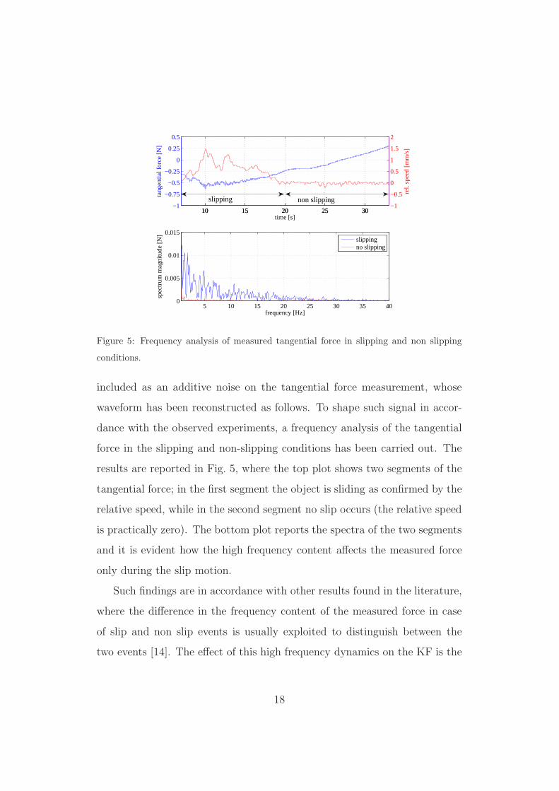
Figure 5: Frequency analysis of measured tangential force in slipping and non slipping

conditions.

included as an additive noise on the tangential force measurement, whose

waveform has been reconstructed as follows. To shape such signal in accor-

dance with the observed experiments, a frequency analysis of the tangential

force in the slipping and non-slipping conditions has been carried out. The

results are reported in Fig. 5, where the top plot shows two segments of the

tangential force; in the first segment the object is sliding as confirmed by the

relative speed, while in the second segment no slip occurs (the relative speed

is practically zero). The bottom plot reports the spectra of the two segments

and it is evident how the high frequency content affects the measured force

only during the slip motion.

Such findings are in accordance with other results found in the literature,

where the difference in the frequency content of the measured force in case

of slip and non slip events is usually exploited to distinguish between the

two events [14]. The effect of this high frequency dynamics on the KF is the

18

0 1 2 3 4 5 6 7 8 9 10−1.5

−1

−0.5

0

0.5

1

time [s]

forc

e [N

]

0 1 2 3 4 5 6 7 8 9 10−1.5

−1

−0.5

0

0.5

1

1.5

rel.

spee

d [m

m/s

]

time [s]

y model.y meas.

fn meas.

0 1 2 3 4 5 6 7 8 9 10−2

−1

0

1

rel.

disp

l. [m

m]

measuredmodelled

measuredmodelled

Figure 6: Experimental-numerical correlation during a stick-slip motion at 0.25Hz with

high frequency dynamics.

same of the disturbances acting on it, thus it can be exploited to detect the

slippage and it will be used in the friction estimation algorithm described in

detail in Section 5.2. Therefore, following the design criteria found in [28,

29], a sensor pad with epidermal micro-ridges has been produced by silicone

molding purposefully to enhance such high frequency dynamics and, as a

consequence, improve the effectiveness of the slipping detection algorithm

based on the monitoring of the KF residual. The presence of such additional

disturbance will also affect the selection of the detection threshold as it will

be explained in Section 4.2.

Therefore, to visualize such behaviour also in the dynamic simulator and

not to improve the real accuracy of the model, the previous simulation has

been repeated by including the high frequency dynamics as identified above

and added as a noise to the tangential force only during slipping motions.

The results are reported in Fig. 6, where both the tangential force and the

19

0 10 20 30 40 50 60 70 80 90−1.5

−1

−0.5

0

0.5

1

time [s]

forc

e [N

]

ft

fn

0 10 20 30 40 50 60 70 80 90−0.04−0.03−0.02−0.01

00.010.020.030.04

time [s]

dete

c. s

igna

l [N

]

0 10 20 30 40 50 60 70 80 90−2−1.5−1−0.500.511.52

rel.

spee

d [m

m/s

]

25 30 35 40 450

0.005

0.01

threshold

slipping slipping slipping slipping

Figure 7: Validation of the slipping detection algorithm.

relative speed are now affected by high frequency components. Note that

the oscillations of the measured relative speed are caused not only by this

high frequency dynamics but mainly by the measurement noise affecting the

displacement sensor, that explains the presence of the oscillations even for

low values of the relative speed, however this is not the case for the measured

tangential force.

It is worth remarking that in order to obtain the good accordance between

the measured and the modelled displacement in the simulations presented so

far it was necessary to include in the dynamic simulator a small asymmetrical

Coulomb friction force acting at the motor shaft of the horizontal voice coil.

4.2. Tuning and validation of the slipping detection algorithm

Once the dynamic model parameters have been refined, an experiment

has been performed to validate the slipping detection algorithm presented in

Section 3 and based on a suitable elaboration of the KF residual. Specifically,

the algorithm detects a slippage if a detection signal is larger than a selected

20

threshold. The detection signal is simply the low-pass filtered version of

the KF residual and its absolute value is then compared to the threshold

to be selected. The filter is aimed at removing from the residual only the

measurement noise at very high frequencies. The bandwidth of the filter is

selected at 5Hz so as to not attenuate most of the high frequency dynamics

appearing during slip motions, and remove the noise at the same time.

During the experiment, under a constant normal force of about 1N, a

periodic tangential force with waveform typical of the exploration phase de-

scribed in Section 5.2, has been applied to the sensor pad by feeding the

horizontal voice coil with an electrical current signal with trapezoidal shape,

whose amplitude is high enough to cause slippage. The results are reported

in Fig. 7. It is clear how during the slip motions, i.e., the time intervals when

the relative speed is not zero, the absolute value of the detection signal is

larger than the threshold Th, which has been selected at 0.005N and verified

to be effective in a number of experiments with different values of the applied

normal force.

21

+

vertical voice coil

horizontal voice coil

Forcesensor

Kalmanfilter

x÷

e

ft

y

fn

y

Ig

It

In

µc

Cs(z)Id

Iskn

Figure 8: Slipping avoidance control scheme.

5. Slipping avoidance algorithm: simulation and experiments

The slipping control scheme proposed in this paper is depicted in Fig. 8.

Basically, the algorithm computes the control signal, i.e., a suitable current

In to feed the vertical voice coil to adjust the normal force component fn.

Such control signal is composed by three contributions. The first one is a

constant value Ig that simply compensates for the weight of the mobile part

of the voice coil and the force sensor placed on its top. The second one Is

generates a normal force with a magnitude high enough to let the force vector

stay within the friction cone; in this way, in static conditions, there should

be no slipping at the contact between the sensor pad and the object. Such

normal force can be easily computed by measuring the actual tangential

force and dividing it by an estimate µc of the friction coefficient. In the

following, a method for obtaining such an estimate will be proposed based on

an initial exploration phase of the object to be manipulated, which precedes

the actual manipulation phase. The third contribution Id corresponds to the

22

portion of the normal force needed to increase the friction force in dynamic

conditions. One of the contributions of the present paper is a method to

calculate such force. In fact, most of the existing methods to avoid slippage

tend to constraint the contact force vector in the friction cone, that means

applying a normal force proportional to the measured tangential force [19,

30], however, this is sufficient only in quasi-static conditions. To ensure

slippage avoidance even in dynamic conditions, e.g. during robotic dynamic

manipulation, a way to compensate also for the inertial forces is needed.

The approach proposed in this work is to exploit the KF residual, which, as

already explained, increases as soon as the disturbance w is not zero, e.g., in

dynamic conditions (see Eq. (20)). Specifically, the control current In of the

vertical voice coil, that applies the grip force, is computed as follows.

In = Is + Id + Ig. (29)

Apart from the current Ig needed to compensate the weight of the vertical

voice coil, the first contribution to the control current is

Is = kn|y|

µc

, (30)

that is proportional to the absolute value of the ratio between the (measured

and filtered by the KF) tangential force y and an estimate of the friction co-

efficient µc. Note that the gain kn is needed to convert a desired normal force

into an electrical current feeding the vertical voice coil and it has been esti-

mated equal to 0.16A/N. In order to reduce the effects of the measurement

noise, the output of the KF y has been used as tangential force rather than

the direct measurement y. A slipping avoidance algorithm that works quite

well in quasi-static conditions composed only by this first part Is has already

been successfully tested in [17] and [15], but it can work only in quasi-static

conditions.

23

The second contribution Id is the absolute value of the slippage controller

Cs(z) output, which is a first-order low-pass filter with a dc gain kc = 5

and a cutoff frequency of 1Hz. The input of the controller is the Kalman

residual e. Note that the absolute value has to be taken in order to ensure

that the normal force is always a pushing force. The controller is basically

a proportional action on the Kalman error whose gain kc is computed as

follows. To avoid slippage even with a changing tangential force, the normal

force corresponding to the control current computed by the controller (apart

from the gravity compensation term) should stay within the friction cone,

i.e., it should exceed the ratio between the tangential force and the minimum

value of the friction coefficient corresponding to the minimum break-away

force as recalled in Section 2, call it µmin, i.e.,

|ft|

µc

+ kc|e| >|ft|

µmin

. (31)

From the above equation one could, of course, choose µc < µmin and kc = 0,

but this would result into unnecessarily high grip forces even in static condi-

tions. Whereas, the proposed idea is to increase the grip force on the basis of

the Kalman error so as to increase the normal force only in the presence of

inertial loads that could cause the slippage, namely when the Kalman resid-

ual e increases. Given a desired minimum error e and a maximum allowed

tangential load ft, the gain kc can be easily computed from Eq. (31) as

kc >ft

e

(

1

µmin

−1

µc

)

. (32)

Assuming, for the following experiments, ft = 0.6N, µmin = 0.12, µc = 0.3

and e = 0.1N, the gain kc = 5 has been computed2. Of course, this approach

2The minimum value for the friction coefficient has been selected assuming a 40%

reduction of the kinetic friction coefficient in quasi-static conditions reported in Tab. 1.

24

is valid under the assumption that all involved signals keep limited. But, this

is certainly verified under the reasonable assumptions of bounded tangential

forces and bounded measurement noise. In fact, in such a case, the KF

always converges since the disturbance w remains bounded as soon as the

normal force is large enough that no relative motion between the object

and the sensor occurs and thus e keeps limited. The cutoff frequency of

the controller should be selected higher than the maximum frequency of

the applied tangential force and low enough to avoid amplification of the

measurement noise. In the following experiments it has been selected equal

to 1Hz since the maximum frequency of the tangential force is assumed

0.5Hz.

5.1. Slipping avoidance experiment with known friction coefficient

A first experiment to evaluate the slippage avoidance control algorithm

has been carried out by applying an external tangential force with a quasi-

sinusoidal signal, i.e., a sinusoid with time-varying frequency and amplitude

in the ranges of [0.1, 0.5] Hz and [0.3, 0.6] N, respectively. The friction co-

efficient has been assumed known in advance and the value µc needed to

compute the control current Is in Eq. (30) has been selected equal to 0.3,

which is the estimated friction coefficient between Teflonr and silicone as

reported in Tab. 1, as said, to limit as much as possible grasp forces. The fre-

quency range has been selected slightly lower than the maximum frequencies

measured in human manipulation tasks as reported in [31]. The amplitude

range has been selected on the basis of the corresponding values of the normal

force needed to avoid slippage, that are in the order of 3 − 6N as it will be

seen, which are very close to the acquired normal forces applied by fingertips

during actual human manipulation tasks such as grasping of bottles, cups

and unscrewing caps, which can be found in [32] and [33].

25

50 60 70 80 90 100 110 120−8

−6

−4

−2

0

time [s]

forc

e [N

]

fn model.

fn meas.

50 60 70 80 90 100 110 120

0

0.5

1

time [s]

rel.

pos.

[mm

]

50 60 70 80 90 100 110 120

0

1

rel.

spee

d [m

m/s

]

modelledmeasured

modelledmeasured

slipping avoidance control ON

Id = 0

Figure 9: Slipping avoidance control experiment and simulation in the case of a known

friction coefficient.

The results are reported in Fig. 9, where the plot on the top shows the

normal force computed by the slipping control algorithm on the basis of a

known friction coefficient and the measured tangential force. The plot on the

bottom shows that the relative speed between the object and the sensor pad

keeps very low while the dynamic slipping avoidance control action is active.

It is important to notice that the position sensor signal, reported in the

same plot, is the superposition of the deformation of the sensor pad and the

actual relative displacement. Taking into account the pad stiffness 4000N/m

and the maximum applied tangential force of 0.6N, such deformation can

be up to 0.15mm. This explains why the relative position signal oscillates

even in absence of slippage (until 98 s). Nevertheless, it is clear from the

position signals that when slippage occurs it has an amplitude much higher

than 0.15mm; moreover, as soon as the control action Id is switched off (at

98 s), even with the static slipping avoidance control action Is still active,

26

50 60 70 80 90 100 110 1200

0.5

1

1.5

time [s]

cont

rol c

urre

nts

[A]

Is+I

g

Id

In

50 60 70 80 90 100 110 120−1

−0.5

0

0.5

1

time [s]

rel.

spee

d [m

m/s

]

model.meas.

Figure 10: Slipping avoidance control experiment and simulation in the case of a known

friction coefficient: control currents (top) and slipping events (bottom).

a slow drift of the relative position starts. This means that the object is

actually sliding over the sensor pad surface, even though the slippage occurs

periodically as confirmed by the high peaks of the relative speed, which has

a large third harmonic as typical of stick-slip motions already evidenced in

Section 4.1. To better appreciate the effect of the dynamic control action

Id, its time history is reported in Fig. 10 together with the static control

actions Is+ Ig and the total control action In. The same figure also shows in

the bottom plot the relative speed with the slipping events clearly indicated.

It is evident that such events occur in correspondence with the minima of

the control current In, which contains only quasi-static terms. This confirms

that in dynamic conditions, a normal force computed on the basis of a well-

known friction coefficient and the sole tangential force is not sufficient to

avoid object slippage. Note that in the figure the simulation results are also

reported in the same case study and they evidently are in a good accordance

27

+ _+

+

µch

µch∆µch

1

1

0

eh LPFshdh αµc

−Th Th νTh−νTh

γµc

z−1

Figure 11: Block scheme of the estimation algorithm of the friction coefficient.

with the experiments.

5.2. Friction estimation algorithm

In order to relax the hypothesis of a known friction coefficient and provide

a good estimate µc of the friction coefficient to the slipping avoidance algo-

rithm presented above, a novel algorithm for friction coefficient estimation is

proposed here and sketched in Fig. 11. It is based on an exploration phase

that has to be carried out, before grasping the object, by rubbing the sensor

pad on the object surface applying a slowly increasing tangential force3 and

activating only the control action Is = kn|y|µc, while Id = 0. Differently from

the experiments already presented, the friction coefficient is being updated

by subtracting to an initial estimation µc a time-varying correction ∆µch,

i.e.,

µch = µc −∆µch. (33)

The correction is updated on the basis of a slipping detection signal dh ob-

tained by applying a low-pass filter to the KF residual eh with a cutoff fre-

quency of 5Hz, which is high enough to not attenuate the high frequency

oscillations occurring during object slipping and low enough to remove the

measurement noise. The signal dh is then converted into a decision signal sh

3The rate of increase should be low enough to get a break-away force high enough to

get a friction coefficient close to the static friction.

28

that is 0 if no correction is necessary or 1 if a correction is needed, i.e., it is

computed as

sh =

0 if |dh| ≤ Th

1 if |dh| > νTh

0.5− 0.5 cos(

πTh(ν−1)

dk −π

ν−1sign(dh)

)

otherwise

, (34)

with Th the threshold already defined in Section 4.2 and ν > 1 is an integer

number that defines the width of a smoothing zone. The smoothing zone has

been introduced to avoid rapid changes in the friction coefficient and thus in

the control normal force. Finally, the correction to the friction coefficient is

computed according to the following update law

∆µch+1=

∆µch + αµcsh if ∆µch ≤ γµc

∆µch otherwise, (35)

where γ ∈ (0, 1) limits the correction to a fraction of the initial estimate

µc and α is the adaptation gain. Note how the minimum friction coefficient

cannot be lower than the value (1− γ)µc.

In order to tune the parameters γ, ν, α of the estimation algorithm, a

simulation study has been carried out on the dynamic model setup in the

previous sections and guidelines for their selection are provided. Specifically,

the haptic exploration test aimed at estimating the contact friction coefficient

has been simulated by applying an increasing tangential force with a fixed

slope to the object in contact with the sensor pad.

The saturation parameter γ is chosen to avoid excessive normal forces

by imposing a lower bound to the friction coefficient µc, the adaptation gain

α and the integer ν have to be selected as a trade off between the need of

gradual changes of µc and the need of a fast learning phase. A lower bound

for the gain α can be easily obtained by assuming that during the manoeuver

29

the decision signal sh is always 1 such that µch reaches the presumed static

friction coefficient µs, namely

µs = µc −α

Tµct ⇒ α =

T

t

(

1−µs

µc

)

, (36)

where T is the sampling time and the initial guess µc has to be selected

higher than µs4 and t is the desired execution time of the exploration phase,

which should be large enough to ensure quasi-static conditions so that the

break-away force is close to the stiction force. Concerning the algorithm

convergence, note that µch can only decrease, thus the applied normal force

is always increasing and so the break-away force. By selecting α larger than

the lower bound in (36), the break-away force will increase at a rate high

enough that the tangential force does not overcome it and the sliding motion

stops, therefore the mean of the Kalman residual eh tends to zero (in practice,

the detection signal dh at the output of the LPF decreases below the threshold

Th selected on the basis of the noise power level) and the computed correction

∆µch becomes constant. The actual value of α has to be tuned experimentally

since the signal sh during the sliding is not constantly equal to 1 because

the detection signal oscillates at the frequency typical of the high frequency

dynamics phenomenon described in Section 4 (see Fig. 5). The gain α should

be also kept small enough to avoid saturation of the estimation algorithm to

the value (1− γ)µc.

Following these guidelines, a simulation of an exploration phase lasting

t = 10 s has been carried out with an initial estimate of the friction coefficient

µc = 0.5, which is much larger than the actual friction coefficient of the

contact with the Teflonr material reported in Tab. 1. With such a large

4In any case, µc should be selected large enough to allow sliding during the initial phase

of the exploration manoeuver.

30

0 10 20 30 40 50 60 70 80 90 100−4

−3

−2

−1

0

1

time [s]

forc

e [N

]

yyfn

0 10 20 30 40 50 60 70 80 90 100

0.2

0.3

0.4

0.5

time [s]

µ c

0 10 20 30 40 50 60 70 80 90 1000

0.005

0.01

0.015

0.02

0.025

0.03

dete

ctio

n si

gnal

[N]

adaptation OFFadaptation ON

threshold

Figure 12: Learning phase of the friction coefficient: simulation.

friction coefficient used to compute the applied normal force, it is expected

that when the amplitude of the tangential force becomes high enough, a

slippage occurs. This is confirmed by the simulation results shown in Fig. 12,

where, in the first 30 seconds when the adaptation is off, a slippage occurs

(see how the detection signal is larger than the threshold). Starting with an

initial value of α = 4·10−5 obtained using Eq. (36) where µs has been selected

equal to the value in Tab. 1, it has been increased until the value 6 · 10−4

at which the algorithm saturates during the exploration time at the value

γµc with γ = 0.7 (which means that the initial friction coefficient estimate

can be decreased down to its 30%). The final value is then selected at the

half of such value, i.e. α = 3 · 10−4, which allows to avoid saturation and

obtain the convergence within the duration of the exploration phase. The

last parameter to select is the smoothing factor ν which has been chosen

equal to 3 as a compromise between speed of convergence and smoothness

of the applied normal force. With such parameters, the adaption algorithm

31

0 10 20 30 40 50 60 70 80 90 100−4

−3

−2

−1

0

1

time [s]

forc

e [N

]

yyfn

0 10 20 30 40 50 60 70 80 90 100

0.2

0.4

time [s]

µ c

0 10 20 30 40 50 60 70 80 90 1000

0.005

0.01

0.015

0.02

0.025

0.03

dete

ctio

n si

gnal

[N]

threshold

adaptation ONadaptation OFF

Figure 13: Learning phase of the friction coefficient: experiment.

is activated after 30 s and the correction to the friction coefficient starts at

40 s as soon as the sliding starts as indicated by the detection signal that

overcomes the threshold. It is evident how during the adaptation, between

40 s and 50 s, the normal force increases at an increasing rate due to the

decreasing value of µch, until the sliding stops and so the update of µch.

Note that the friction coefficient has been reduced to a value in between the

static and kinetic friction coefficients reported in Tab. 1, i.e., about 0.24. This

is what is typically done in robotic grasping tasks to avoid object slippage,

namely constraining the contact force vector to stay within the friction cone

by using a friction coefficient lower than the static friction [30, 3]. The

simulation continues to show that with the friction coefficient so corrected no

further slippage occurs (the detection signal is always far below the threshold)

and thus no correction is computed by the adaptive law.

To validate the estimation algorithm described so far, the same haptic

exploration procedure has been experimentally executed using the same pa-

32

0 20 40 60 80 100 120−8

−6

−4

−2

0

2

time [s]

forc

e [N

]

yyfn

0 20 40 60 80 100 120−0.4

−0.2

0

0.2

0.4

time [s]

rel.

spee

d [m

m/s

], µ c

0 20 40 60 80 100 120−0.75

−0.5

−0.25

0

0.25

0.5

0.75

1

filte

r re

sid.

[N]

slipping avoidance control ONcontrol OFF

learning of the friction coefficient

µc

Figure 14: Final experiment: preliminary exploration phase (0− 38 s), full slipping avoid-

ance control on (38− 98 s), dynamic slipping avoidance control off (98− 120 s).

rameters tuned in simulation. The results are reported in Fig. 13 where the

system behaviour is practically the same of that obtained in simulation. The

final value of the estimated friction coefficient is 0.21 with a difference of 12%

with respect to the simulation.

5.3. Slipping avoidance experiment with unknown friction coefficient

The features of all the algorithms presented in the paper are now high-

lighted by showing the results of a single experiment composed by three

phases. In the first phase the initial friction coefficient estimate is adapted

to the actual contact feature by executing a preliminary exploration proce-

dure with the same parameters used in the previous experiment, i.e., ac-

tivating the static slippage control action Is and not the dynamic one Id,

but starting from an initial guess µc = 0.4. The adaptive law, activated

during the first slippage occurring between 10 s and 20 s, computes correc-

tions ∆µch leading to a final value of µc ≃ 0.26. At about 38 s the second

33

phase starts, i.e., the dynamic slipping avoidance is turned on. At the same

time, a pseudo-sinusoidal tangential force with time-varying amplitude and

frequency is applied to the object and the whole control current In in (29) is

applied to the vertical voice coil resulting into a time-varying normal force

that increases and decreases not only in correspondence with the tangential

force y but also on the basis of the KF residual (reported in Fig. 14 on the

right vertical axis in red) that is significantly different from zero in dynamic

conditions. Such normal force is effective in avoiding the object slippage dur-

ing this phase as proved by the small measured relative speed (reported in

blue on the left vertical axis of the figure). The third phase of the experiment

starts at approximately 98 s, when the dynamic slipping avoidance control

action is turned off and only the static one is left active, while a sinusoidal

tangential force with fixed amplitude and frequency is applied to the object.

The relative speed is significantly larger than in the second phase and again

with a deformed waveform typical of stick-slip motion, implying that slippage

occurs periodically.

6. Conclusions

The paper proposed a novel method for slipping detection and avoidance

based on a Kalman filter designed on the basis of a dynamic model describing

the contact behaviour between a compliant force sensor pad and a manipu-

lated object. The slipping detection algorithm is exploited in a preliminary

haptic exploration phase of the object surface to on-line estimate the actual

friction coefficient at the contact through an adaptive strategy. Based on

the estimated friction coefficient and the KF residual, the slipping avoidance

control law is able to adjust the grip force both in quasi-static and dynamic

conditions.

34

A limitation of the proposed approach is that the slipping control strategy

is effective only under the assumption that the actual friction coefficient does

not change during the manipulation. Future work will be devoted to relax

such assumption, e.g. by suitable filtering of the Kalman residual that should

allow to distinguish between slippage due to friction coefficient changes and

dynamic effects. Furthermore, currently, the analysis has been performed

only with reference to contact forces, ignoring contact moments, assuming

that only translations can occur. Therefore, future work will be devoted to

extend such approach to torsional moments that build up when distributed

contacts occur and rotations are allowed. Finally, the commercial force sensor

will be substituted with a force/tactile sensor specifically designed to be

integrated into a robotic hand for testing the proposed algorithms in a real

robotic manipulation task.

Acknowledgments

The research leading to these results has been funded by the Italian Min-

istry of University and Research (MIUR), grant PRIN2009 “ROCOCO”.

References

[1] R. D. Howe, Tactile sensing and control of robotic manipulation, Journal

of Advanced Robotics 8 (3) (1994) 245–261.

[2] I. Birznieks, M. K. O. Burstedt, B. B. Edin, R. S. Johansson, Mecha-

nisms for force adjustments to unpredictable frictional changes at indi-

vidual digits during two-fingered manipulation, Journal of Neurophysi-

ology 80 (4) (1998) 19892002.

[3] M. R. Tremblay, M. R. Cutkosky, Estimating friction using incipient

slip sensing during a manipulation task, in: Proc. of the 1993 IEEE

35

Int. Conference on Robotics and Automation, Atlanta, GA, 1993, pp.

429–434.

[4] N. Xydas, I. Kao, Modeling of contact mechanics and friction limit sur-

faces for soft fingers in robotics, with experimental results, The Inter-

national Journal of Robotics Research (1999) 941950.

[5] T. Maeno, T. Kawamura, S. Cheng, Friction estimation by pressing an

elastic finger-shaped sensor against a surface, IEEE Trans. on Robotics

and Automation 20 (2) (2004) 222–228.

[6] K. Nakamura, H. Shinoda, Tactile sensing device instantaneously eval-

uating friction coeffcients, in: Proc. of the 18th Sensor Symposium,

Kawasaki, J, 2001, pp. 151–154.

[7] P. Dahl, A solid friction model, Tech. Rep. TOR-0158H3107-18I-1, The

Aerospace Corporation, El Segundo, CA (1968).

[8] J. Swevers, F. Al-Bender, C. Ganseman, T. Prajogo, An integrated fric-

tion model structure with improved presliding behaviour for accurate

friction compensation, IEEE Trans. on Automatic Control 45 (4) (2000)

675–686.

[9] C. Canudas de Wit, H. Olsson, K. J. Astrom, P. Lishinsky, A new model

for control of systems with friction, IEEE Trans. on Automatic Control

40 (5) (1995) 419–425.

[10] K. J. Astrom, C. Canudas de Wit, Revisiting the lugre friction model:

Stick-slip motion and rate-dependence, IEEE Control Systems Magazine

28 (6) (2008) 101–114.

36

[11] X. Song, H. Liu, J. Bimbo, K. Althoefer, L. D. Seneviratne, Object

surface classification based on friction properties for intelligent robotic

hands, in: Proc. of World Automation Congress WAC 2012), Puerto

Vallarta, MX, 2012, pp. 1–5.

[12] G. Ferretti, G. Magnani, P. Rocco, Modular dynamic modeling and

simulation of grasping, in: Proc. of the 1999 IEEE/ASME Int. Conf. on

Advanced Intelligent Mechatronics, Atlanta, GA, 1999, pp. 428–433.

[13] M. T. Francomano, D. Accoto, E. Guglielmelli, Artificial sense of slip-a

review, IEEE Sensors Journal 13 (7) (2013) 2489–2498.

[14] M. Vatani, E. D. Engeberg, J.-W. Choi, Force and slip detection

with direct-write compliant tactile sensors using multi-walled carbon

nanotube/polymer composites, Sensors and Actuators A: Physical 195

(2013) 90–97.

[15] G. De Maria, C. Natale, S. Pirozzi, Slipping control through tactile

sensing feedback, in: Proc. of the 2013 IEEE Int. Conf. on Robotics and

Automation, Karlsruhe, DE, 2013, pp. 3508–3513.

[16] G. De Maria, C. Natale, S. Pirozzi, Tactile data modelling and interpre-

tation for stable grasping and manipulation, Robotics and Autonomous

Systems 61 (2013) 1008–1020.

[17] G. De Maria, C. Natale, S. Pirozzi, Tactile sensor for human-like manip-

ulation, in: Proc. of the 2012 IEEE RAS/EMBS Int. Conf. on Biomed-

ical Robotics and Biomechatronics, Rome, I, 2012, pp. 1686–1691.

[18] B. Heyneman, M. R. Cutkosky, Slip interface classification through tac-

tile signal coherence, in: Proc. of the 2013 IEEE/RSJ Int. Conference

on Intelligent Robots and Systems, Tokyo, 2013, pp. 801–808.

37

[19] E. D. Engeberg, S. G. Meek, Adaptive sliding mode control for pros-

thetic hands to simultaneously prevent slip and minimize deformation

of grasped objects, IEEE/ASME Trans. on Mechatronics 18 (1) (2013)

376–385.

[20] J. Ueda, A. Ikeda, T. Ogasawara, Grip-force control of an elastic object

by vision-based slip-margin feedback during the incipient slip, IEEE

Trans. on Robotics 21 (6) (2005) 1139–1147.

[21] G. De Maria, C. Natale, S. Pirozzi, Force/tactile sensor for robotic ap-

plications, Sensors and Actuators A: Physical 175 (2012) 60–72.

[22] V. I. Johannes, M. A. Green, C. A. Brockley, The role of the rate of

application of the tangential force in determining the static force coeffi-

cient, Wear 24 (1973) 381–385.

[23] R. S. Dahiya, G. Metta, M. Valle, G. Sandini, Tactile sensing-from hu-

mans to humanoids, IEEE Trans. on Robotics 26 (2010) 1–20.

[24] J. Fishel, G. Loeb, Bayesian exploration for intelligent identification of

textures, Frontiers in Neurorobotics 6 (2012) 1–20.

[25] A. D’Amore, G. De Maria, L. Grassia, C. Natale, S. Pirozzi, Silicone-

rubber-based tactile sensors for the measurement of normal and tangen-

tial components of the contact force, Journal of Applied Polymer Science

122 (6) (2011) 3758–3770.

[26] C. H. Lin, T. W. Erickson, J. A. Fishel, N. Wettels, G. E. Loeb, Sig-

nal processing and fabrication of a biomimetic tactile sensor array with

thermal, force and microvibration modalities, in: Proc. of the IEEE In-

ternational Conference on Robotics and Biomimetics, 2009, pp. 129–134.

38

[27] B. N. J. Persson, Sliding Friction: Physical Principles and Applications,

Springer-Verlag, Berlin, DE, 1998.

[28] Y. Zhang, Sensitivity enhancement of a micro-scale biomimetic tactile

sensor with epidermal ridges, Journal of Micromechanics and Microengi-

neering 20 (2010) 1–7.

[29] J. J. Cabibihan, H. Lin Oo, S. Salehi, Effect of artificial skin ridges on

embedded tactile sensors, in: Proc. of the IEEE Haptics Symposium

2012, Vancouver, BC, 2012, pp. 439–442.

[30] C. Melchiorri, Slip detection and control using tactile and force sensors,

IEEE/ASME Trans. on Mechatronics 5 (3) (2000) 235–242.

[31] F. Gao, M. L. Latash, V. M. Zatsiorsky, Internal forces during object

manipulation, Experimental Brain Research 165 (1) (2005) 69–83.

[32] P. Falco, A kinetostatic data fusion system for observation of human

manipulation, PhD Thesis, Seconda Universita degli Studi di Napoli.

URL http://research.diii.unina2.it/acl/docs/ThesisFalco.pdf

[33] A. Cavallo, P. Falco, On-line segmentation and classification of manip-

ulation actions from the observation of kinetostatic data, IEEE Trans.

on Human-Machine Systems (2013) accepted for publication.

List of Figures

1 Sketch of the contact model: tangential dynamics. . . . . . . . 6

2 The experimental setup. . . . . . . . . . . . . . . . . . . . . . 13

3 Experimental-numerical correlation during a stick-slip motion

at 0.25Hz. . . . . . . . . . . . . . . . . . . . . . . . . . . . . . 16

39

4 Modelling errors during a stick-slip motion at 0.25Hz. . . . . . 17

5 Frequency analysis of measured tangential force in slipping

and non slipping conditions. . . . . . . . . . . . . . . . . . . . 18

6 Experimental-numerical correlation during a stick-slip motion

at 0.25Hz with high frequency dynamics. . . . . . . . . . . . . 19

7 Validation of the slipping detection algorithm. . . . . . . . . . 20

8 Slipping avoidance control scheme. . . . . . . . . . . . . . . . 22

9 Slipping avoidance control experiment and simulation in the

case of a known friction coefficient. . . . . . . . . . . . . . . . 26

10 Slipping avoidance control experiment and simulation in the

case of a known friction coefficient: control currents (top) and

slipping events (bottom). . . . . . . . . . . . . . . . . . . . . . 27

11 Block scheme of the estimation algorithm of the friction coef-

ficient. . . . . . . . . . . . . . . . . . . . . . . . . . . . . . . . 28

12 Learning phase of the friction coefficient: simulation. . . . . . 31

13 Learning phase of the friction coefficient: experiment. . . . . . 32

14 Final experiment: preliminary exploration phase (0 − 38 s),

full slipping avoidance control on (38−98 s), dynamic slipping

avoidance control off (98− 120 s). . . . . . . . . . . . . . . . . 33

40