sensors

Article

Features of Invariant Extended Kalman Filter Appliedto Unmanned Aerial Vehicle Navigation

Nak Yong Ko 1,* ID , Wonkeun Youn 2, In Ho Choi 2, Gyeongsub Song 3 and Tae Sik Kim 2

1 Department of Electronic Engineering, Chosun University, 375 Seosuk-dong Dong-gu,Gwangju 501-759, Korea

2 Korea Aerospace Research Institute, Daejon 34133, Korea; wkyoun@kari.re.kr (W.Y.);inho@kari.re.kr (I.H.C.); kts@kari.re.kr (T.S.K.)

3 Department of Control and Instrumentation Engineering, Chosun University, 375 Seosuk-dong Dong-gu,Gwangju 501-759, Korea; sgs0369@naver.com

* Correspondence: nyko@chosun.ac.kr; Tel.: +82-42-870-3512

Received: 28 June 2018; Accepted: 23 August 2018; Published: 29 August 2018�����������������

Abstract: This research used an invariant extended Kalman filter (IEKF) for the navigation of anunmanned aerial vehicle (UAV), and compared the properties and performance of this IEKF with thoseof an open-source navigation method based on an extended Kalman filter (EKF). The IEKF is a fairlynew variant of the EKF, and its properties have been verified theoretically and through simulationsand experiments. This study investigated its performance using a practical implementation andexamined its distinctive features compared to the previous EKF-based approach. The test used twodifferent types of UAVs: rotary wing and fixed wing. The method uses sensor measurements of thelocation and velocity from a GPS receiver; the acceleration, angular rate, and magnetic field from amicroelectromechanical system-attitude heading reference system (MEMS-AHRS); and the altitudefrom a barometric sensor. Through flight tests, the estimated state variables and internal parameterssuch as the Kalman gain, state error covariance, and measurement innovation for the IEKF methodand EKF-based method were compared. The estimated states and internal parameters showedthat the IEKF method was more stable and convergent than the EKF-based method, although theestimated locations, velocities, and altitudes of the two methods were comparable.

Keywords: invariant extended Kalman filter; unmanned aerial vehicle; location; attitude; velocity;GPS; MEMS-AHRS; Kalman gain; error covariance; innovation; estimation

1. Introduction

The invariant extended Kalman filter is a fairly recent development that improves the extendedKalman filter using the geometrically transformed state error and output error based on the Liegroup theory [1]. It could be regarded as an extension and generalization of the multiplicativeextended Kalman filter [2–5]. It can be derived and applied using either the abstract Lie group [6]or matrix Lie group formulation [7]. Derivations of the invariant extended Kalman filter (IEKF)for use in the navigation of an unmanned aerial vehicle using measurements of the location andvelocity from a GPS; the angular rate, acceleration, and magnetic field from a microelectromechanicalsystem-attitude heading reference system (MEMS-AHRS); and the altitude from a barometric sensorhave been reported [2,8]. These were based on the abstract Lie group approach. A matrix Lie groupformulation of the IEKF was used for simultaneous localization and mapping (SLAM) and improvedthe consistency of the estimation compared to the EKF-based SLAM method [9].

The IEKF approach has several distinctive advantageous features compared to the usualEKF-based approaches: (1) a symmetry preserving observer, (2) sound geometric structures for

Sensors 2018, 18, 2855; doi:10.3390/s18092855 www.mdpi.com/journal/sensors

Sensors 2018, 18, 2855 2 of 26

quaternion estimation, and (3) a large expected domain of convergence [8]. The IEKF-based methodpreserves the norm of the estimated quaternion as a unit. In contrast, the prediction and correctionprocedures of the usual EKF break the unit norm constraint on the quaternion for the attitude.In addition, the approximation to a linear system of a nonlinear process and measurement modelsometimes induces an unstable and divergent estimation. The IEKF relieves this problem by extendingthe state space where convergence is preserved.

The IEKF is basically an invariant observer which adopts an EKF approach for determiningobserver gain to take advantage of the convergence property of the linear Kalman filter. The propertyof invariant, or otherwise called symmetry-preserving system had been used for control applications [10].Aghannan and Rouchon [11] initially exploited the invariance property for observer or estimator designresulting in an invariant observer. Though the invariant observer proposed in [11] was the predecessorof the IEKF, it did not incorporate the idea of EKF. The invariant observer was further developedand convergence property was verified by numerical simulation using a mechanical system of balland beam [12]. Martin et al. introduced invariant output error in their development of an invarianttracking method [13]. Though the invariant output error was proposed and used for control use,it played an important role in development of IEKF later [14]. The invariant observer was theoreticallyfurther investigated, providing the foundations for development into IEKF, especially for navigationapplications [15]. Finally, IEKF was proposed by incorporating the EKF methodology into the invariantobserver for determining the observer gain [14]. It should be noticed that the IEKF does not use directlinearization of nonlinear process model and measurement model, unlike the usual EKF [16]. This willbe discussed in Section 3.1 along with the explanation about the linearization process.

Studies on the IEKF have demonstrated the feasibility of using it for aerial, indoor, and roadnavigation [17]. The IEKF and EKF were applied for SLAM, and a comparison of their resultsproved that the IEKF improved the estimation convergence and consistency compared to the EKF [18].The comparison used simulated data. The IEKF was also used for helicopter unmanned aerial vehicle(UAV) navigation [19], and its estimation performance was found based on experimental results,focusing on the estimated data of the state variables, excluding internal parameters such as the Kalmangain, state error covariance, and measurement innovation. The IEKF was also compared with themultiplicative extended Kalman filter (MEKF) [2,8,20]. Barczyk et al. compared the IEKF with theMEKF for indoor localization using scan matching point clouds captured by a low-cost Kinect depthcamera [20]. They used experimental results and compared the Kalman gain for the case of indoornavigation. Barczy and Lynch applied the IEKF to a magnetometer-plus-GPS-aided inertial navigationsystem for a helicopter UAV, and presented experimental data on the estimated state variables [21].

This study concentrated on supporting the availability of IEKF navigation by a comparison andanalysis of the estimation results from flight tests of UAVs, which are widely used. Experimentsusing two UAVs, a fixed wing UAV and a rotary wing UAV, compared the features of the IEKFand conventional EKF. In particular, this study compares the internal parameters of the Kalmangain, state error covariance, and measurement innovation to explicitly show the features of theIEKF. Theoretical derivations and simulations have verified the features of the IEKF in numerousstudies [1,6–8]. However, studies investigating and analyzing the estimation results and internalparameters through practical applications were not sufficient to validate the feasibility of usingthe IEKF in a wide range of applications. In studies where experimental results were compared,they usually concentrated on the estimated results of state variables, excluding internal parameterssuch as the Kalman gain, state error covariance, and measurement innovation [19].

Section 2 lists the notations used to describe the IEKF-based navigation methods. Section 3briefly describes the IEKF-based navigation method used in this research, and also explains theEKF-based method that was used for comparison. Section 4 provides details of the experimentsusing a fixed wing UAV and quadrotor to verify and compare the methods. Section 5 compares anddiscusses the properties revealed from the experiments. This section compares the estimation resultsfor the state variables and internal parameters such as the Kalman gain, state error covariance, and

Sensors 2018, 18, 2855 3 of 26

measurement innovation. Finally, Section 6 provides some concluding remarks and possible futureresearch directions related to the current research.

2. Nomenclature

The following nomenclature is used in the paper.

q(t) attitude represented by quaternion at time t: q(t) =(q0(t), qx(t), qy(t), qz(t)

)T

where q0(t) is the scalar part and (qx(t), qy(t), qz(t)) is the vector part of the quaternionx(t) location at time t: x(t) = (x(t), y(t), z(t))T

v(t) velocity at time t: v(t) = dx(t)dt =

(vx(t), vy(t), vz(t)

)T

ω(t) rotational velocity measured by gyroscope in the instrument coordinate frame at time t:ω(t) =

(ωx(t), ωy(t), ωz(t)

)T

a(t) acceleration measured in the instrument coordinate frame at time t:a(t) = (ax(t), ay(t), az(t))T

zx(t) measurement of location at time t: zx(t) = (zx(t), zy(t), zz(t))T

zv(t) measurement of velocity at time t: zv(t) = (zvx (t), zvy (t), zvz (t))T

zm(t) measurement of magnetic field in the instrument coordinate frame at time t:zm(t) = (zmx (t), zmy (t), zmz (t))

T

zh(t) measurement of altitude at time tbh(t) bias in altitude measurement at time t: zh(t) = z(t) + bh(t)

bω(t) bias in angular rate measurement at time t: bω(t) =(

bωx (t), bωy (t), bωz (t))T

sa(t) scale factor in acceleration measurement at time tg gravitational acceleration regarded as constant throughout the implementation

in the northeast down (NED) coordinate systemm geomagnetic field appropriate for a location in the NED coordinate frame that is considered

to be constant throughout the experiment: m = (mx, my, mz)T

ed 3× 1 unit vector in the direction d, where d ∈ {x, y, z}

In the following description, time index (t) will be omitted from the notations if there arises noambiguity without index (t) in the context. Since the AHRS measures acceleration and angular rate aswell as the magnetic field, it is also considered that AHRS includes inertial measurement unit (IMU).Thus, in this paper, IMU measurement means the acceleration and angular rate measured by AHRS.

3. IEKF and ecl-EKF for UAV Navigation

This section briefly describes the IEKF-based navigation method adopted in this research and theEKF-based method that was used for comparison. Two IEKF methods were used: one for estimatingthe location, attitude, and velocity [2], and the other for estimating the attitude and velocity [8].Both of them specifically used right IEKF methods and were from [2,8], respectively. The method to becompared with the IEKF methods was the EKF from the estimation and control library (ECL) of thePX4 project [22], which will be called the ecl-EKF from now on. Hereafter, the IEKF used for estimatingthe location, attitude, and velocity will be called the IEKF-lav, while the IEKF for the attitude andvelocity will be called the IEKF-av.

3.1. IEKF-lav: Right IEKF for Estimation of Location, Attitude, and Velocity

The right IEKF used for estimating the attitude, velocity, and location is first described [2].The state vector χ to be estimated consists of the state variables shown in Equation (1):

χ = (q, v, x, bω, sa, bh)T . (1)

The state is subject to the process model shown as a differential Equation (2):

Sensors 2018, 18, 2855 4 of 26

χ =

qvx

bω

sa

bh

=

12 q ∗ (ω− bω)

g + 1sa

q ∗ a ∗ q−1

v000

. (2)

The measurements include the velocity and location from the GPS, altitude from a barometricsensor, and magnetic field from a magnetometer in the MEMS-AHRS as follows: z = (zv, zx, zh, zm)T .The measurements are related to the state as shown by the measurement model (3):

z =

zv

zx

zhzm

=

vx

x · ez + bhq−1 ∗m ∗ q

. (3)

In the application of the right IEKF, the process and measurement model incorporates processnoise w =

(wq, wv, wx, wbω

, wsa , wbh

)T and measurement noise ν = (νv, νx, νh, νm)T in models (2)and (3), resulting in Equations (4) and (5):

χ =

qvx

bω

sa

bh

=

12 q ∗ (ω− bω)

g + 1sa

q ∗ a ∗ q−1

v000

+

Mqwq ∗ qMvwv

Mxwx

q−1 ∗Mbωwbω

∗ qsaMsa wsa

Mbhwbh

(4)

z =

zv

zx

zhzm

=

v + Nvνv

x + Nxνx

x · ez + bh + Nhνhq−1 ∗ (m + Nmνm) ∗ q

. (5)

The inclusion of noise in the process and measurement model, as shown in Equations (4) and (5),transforms the problem for the application of the IEKF, and the IEKF estimates the state and errorcovariance P as shown in Equations (6) and (7), respectively:

˙χ =

˙q˙v˙x

˙bω

˙sa˙bh

=

12 q ∗

(ω− bω

)g + 1

saq ∗ a ∗ q−1

v000

+

KqE ∗ qKvEKxE

q−1 ∗KbωE ∗ q

saKsa EKbh

E

, (6)

P = AP + PAT + MMT − PCT(NNT)−1CP, (7)

where process error covariance M and measurement error covariance N are given in Equation (8):

M = Diag(Mq, Mv, Mx, Mbω, Msa , Mbh

),N = Diag(Nv, Nx, Nh, Nm).

(8)

In Equations (6) and (7) for the state χ and error covariance P, the Kalman gain K and outputerror E are given by Equations (9) and (10), respectively:

Sensors 2018, 18, 2855 5 of 26

K = −(Kq, Kv, Kx, Kbω, Ksa , Kbh

)T = PCT(NNT)−1, (9)

E =

zv − zv

zx − zx

zh − zhm− q ∗ zm ∗ q−1

=

v− v−Nvνv

x− x−Nxνx

(x− x) · ez + bh − bh −Nhνhm− q ∗ q−1 ∗ (m + Nmνm) ∗ q ∗ q−1

. (10)

The calculation of Kalman gain K and state error covariance P requires linearized state transitioncoefficient A and measurement coefficient C as shown in Equations (7) and (9). Usual EKF takes thepartial derivatives of process model and measurement model with respect to state as the matrices A andC, respectively. On the contrary, IEKF finds the matrices A and C in a different way from the usual EKFbecause the IEKF takes state error differently from that of the usual EKF [8,16]. To make the observerinvariant and adapt the problem for IEKF application, the state error η = (ηq, ηv, ηx, ηbω

, ηsa, ηbh

)T istaken as Equation (11) [2]:

ηqηvηx

ηbω

ηsa

ηbh

=

q ∗ q−1

v− vx− x

q ∗(

bω − bω

)∗ q−1

sasa

bh − bh

. (11)

Unlike the usual EKF where state error is taken as the algebraic difference between estimatedstate and true state, the state error in IEKF has a different form as shown at the first, fourth, and fifthcomponents of the state error vector in Equation (11).

For usual EKF, the system equation for state error differential, which is derived from the stateestimation equation for usual EKF and the usual process model, is shown as Equation (12) [8]:

δη = (A−KC)δη−Mw + KNν. (12)

Likewise, for the IEKF, the system equation for state error differential η can be found by combiningEquations (4), (6), (10), and (11). Linearizing the system equation for state error differential η of the IEKFand dropping all the quadratic terms for the noise and infinitesimal state error results in a linearizedstate error differential system, which is equivalent to Equation (12). Finding the correspondencebetween the linearized state error differential system for IEKF and Equation (12) for usual EKFyields the linearized process transition coefficient A and measurement coefficient C for IEKF asEquations (13) and (14), respectively [2]:

A =

033 033 033 − 12 I3 031 031

−2Ia× 033 033 033 −Ia 031

033 I3 033 033 031 031

033 033 033 Iω× 031 031

013 013 013 013 011 011

013 013 013 013 011 011

, (13)

C =

033 I3 033 033 031 031

033 033 I3 033 031 031

013 013 eTz 013 011 −I1

2m× 033 033 033 031 031

. (14)

In A and C, the invariant quantities Iω and Ia are given in the following Equation (15):

Sensors 2018, 18, 2855 6 of 26

Iω = q ∗(

ω− bω

)∗ q−1,

Ia = 1sa

q ∗ a ∗ q−1.(15)

I× is defined such that I×u = I× u for all u ∈ R3.It should be noticed that matrices A and C are constant if invariant quantities Iω and Ia are constant.

Iω and Ia are constant if the UAV flies at a constant angular rate and there is constant acceleration inthe NED coordinate frame. If these conditions are met, the IEKF becomes a linear Kalman filter, whichguarantees convergence. This is one of the most distinctive features of the IEKF compared with theusual EKF. In addition, the differential equation for the quaternion estimation derived in Equation (6)intrinsically keeps the estimated quaternion normalized at all times. These advantageous features applyto all IEKFs, including the IEKF-av, which will be described in Section 3.2.

In case of usual EKF, the matrices A and C are derived from partial derivatives of process modeland measurement model. Since the process model and measurement model are a nonlinear combinationof attitude, angular rate, acceleration, bias in angular rate, and acceleration scale factor, the partialderivatives depend on those variables in a nonlinear manner, and vary with a change of those variables,which is not desirable for convergence. If all the variables are constant, the matrices A and C will beconstant and the EKF also will work like a linear KF, assuring convergence. However, even though theUAV flies at a constant angular rate and constant acceleration in the NED coordinate frame, the matricesA and C are not constant, that is, nonlinear dynamics do not become linear, therefore the propertiesapplicable to linear KF do not apply. On the contrary, in IEKF, the matrices A and C are constant insuch a systematic way that A and C become constant if the UAV flies at a constant angular rate andconstant acceleration in the NED coordinate frame as explained above. This advantage of IEKF overusual EKF is due to the use of invariance property in derivation of the IEKF [8,16].

Putting the above descriptions together, IEKF formulates the process model and measurementmodel to be invariant as Equations (4) and (5), thus making it possible to design the observer [estimator]to be invariant as Equation (6). Due to the invariance property of the observer (6), the sufficientcondition for constant A and C becomes that invariant quantities Iω and Ia be constant. This sufficientcondition for IEKF is relaxed compared with that for the usual EKF, for which attitude, angular rate,acceleration, bias in angular rate, and acceleration scale factor are required to be constant to keepA and C constant—thus formulating the process and measurement model in an invariant way anddesigning the observer to be invariant result in improved convergence property of the IEKF over theusual EKF [8].

In addition to the advantage of convergence property, the quaternion estimation q of the IEKFintrinsically keeps the unit norm constraint onto the quaternion. The magnitude ‖q‖ of the estimatedquaternion is kept as a unit since the quaternion estimate obeys the differential equation presented atthe first component of the observation Equation (6) [8], which is rephrased as Equation (16):

˙q =12

q ∗(

ω− bω

)+ KqE ∗ q. (16)

The second term KqE ∗ q of Equation (16), which is multiplication of quaternion q with thevector KqE, plays the role of preserving the magnitude of the quaternion constant [8]. In usual EKF,the corresponding term will be replaced by the multiplication of Kalman gain with measurementinnovation. Therefore, the magnitude of the estimated quaternion deviates from the unit, thus invalidadjustment of the quaternion to rescale the magnitude to be a unit is inevitable. This deterioratesestimation performance of the usual EKF compared with the IEKF.

3.2. IEKF-av: Right IEKF for Estimation of Attitude and Velocity

This section describes the right IEKF used for estimating the attitude and velocity [8]. The statevector χ to be estimated consists of four variables: the attitude, velocity, bias in the angular ratemeasurement, and scale factor of the acceleration measurement (17):

Sensors 2018, 18, 2855 7 of 26

χ = (q, v, bω, sa)T . (17)

The process model for the state transition is the same as Equation (2), except that two equationsfor the location x and bias in the altitude measurement bh are deleted, resulting in Equation (18):

χ =

qv

bω

sa

=

12 q ∗ (ω− bω)

g + 1sa

q ∗ a ∗ q−1

00

. (18)

The measurements include the velocity from the GPS and the magnetic field from themagnetometer in the MEMS-AHRS as follows: z = (zv, zm)T . Therefore, the measurement modelis derived from that for the IEKF-lav (Equation (3)) by deleting the equations corresponding to theposition and altitude measurements, resulting in Equation (19):

z =

(zv

zm

)=

(v

q−1 ∗m ∗ q

)(19)

The inclusion of process noise is the same as that for the IEKF-lav, except that the equations forthe states of the position and bias in the altitude measurement are deleted from Equation (2). Likewise,the noise incorporated measurement model is just Equation (5), except that the equations for zx and zhare deleted. The process model and measurement model for the IEKF-av are Equations (20) and (21):

χ =

qv

bω

sa

=

12 q ∗ (ω− bω)

g + 1sa

q ∗ a ∗ q−1

00

+

Mqwq ∗ q

Mvwv

q−1 ∗Mbωwbω

∗ qsaMsa wsa

, (20)

z =

(zv

zm

)=

(v + Nvνv

q−1 ∗ (m + Nmνm) ∗ q

). (21)

The IEKF estimator for the attitude and velocity becomes the observer of Equation (22), and thecorresponding error covariance P is determined by Equation (23):

˙χ =

˙q˙v

˙bω

˙sa

=

12 q ∗

(ω− bω

)g + 1

saq ∗ a ∗ q−1

00

+

KqE ∗ q

KvEq−1 ∗Kbω

E ∗ qsaKsa E

, (22)

P = AP + PAT + MMT − PCT(NNT)−1CP, (23)

where process error covariance M and measurement error covariance N are given in Equation (24):

M = Diag(Mq, Mv, Mbω, Msa),

N = Diag(Nv, Nm).(24)

In Equations (22) and (23) for state χ and error covariance P, the Kalman gain K and output errorE are given by Equations (25) and (26), respectively:

K = −(Kq, Kv, Kbω, Ksa)

T = PCT(NNT)−1, (25)

E =

(zv − zv

m− q ∗ zm ∗ q−1

)=

(v− v−Nvνv

m− q ∗ q−1 ∗ (m + Nmνm) ∗ q ∗ q−1

). (26)

Sensors 2018, 18, 2855 8 of 26

To derive the linearized process model A and measurement model C, which are required forcalculating the Kalman gain K and state error covariance P, the state error η = (ηq, ηv, ηbω

, ηsa)T is

taken as Equation (27): ηqηv

ηbω

ηsa

=

q ∗ q−1

v− v

q ∗(

bω − bω

)∗ q−1

sasa

. (27)

Linearizing the state error differential system and fitting the linearized model to Equation (12)yields matrices A and C, as shown in Equations (28) and (29) [8], respectively:

A =

033 033 − 1

2 I3 031

−2Ia× 033 033 −Ia

033 033 Iω× 031

013 013 013 011

, (28)

C =

(033 I3 033 031

2m× 033 033 031

). (29)

3.3. ecl-EKF for Estimation of Attitude, Velocity, and Location

An EKF for estimating the attitude, velocity, and location, called the ecl-EKF, is used forcomparison purposes [23]. The ecl-EKF is an EKF-based navigation algorithm that was developedby the PX4 project [22]. The ecl-EKF sets a state vector encompassing the following 24 statevariables: the attitude by quaternion, velocity, position, IMU delta angle bias, IMU delta velocity bias,earth magnetic field, magnetometer bias, and horizontal wind velocity. It uses measurements of theangular rate and acceleration by the IMU, along with the GPS position, GPS velocity, pressure altitude,and geomagnetic field.

The ecl-EKF uses an output predictor and data buffer to fuse data from sensors with differenttime delays and data rates. The EKF interacts with the strap down inertial navigation unit, data buffer,and output predictor. The ecl-EKF is capable of fusing a large range of different sensor types. It alsodetects outliers in sensor measurements. The ecl-EKF code can be found at GitHub [24]. For theimplementation and details of the ecl-EKF and PX4, please refer to the documents on PX4 at thesite [25].

4. Implementation for Navigation of UAVs

The IEKF methods and ecl-EKF were implemented for the navigation of a four-rotary wing UAV,otherwise called a quadrotor, and a fixed wing UAV. The fixed wing UAV was used to test the IEKF-lavand ecl-EKF, and the quadrotor was used to test the IEKF-av and ecl-EKF. Figure 1 shows the quadrotorand fixed wing UAV used for the flight test. Each UAV had a global navigation satellite system (GNSS),an AHRS, and a barometric altimeter. Tables 1 and 2 explain the UAVs used for the tests, and Table 3lists the performance of the GNSS used in the experiments.

The two UAVs use the same flight control unit of Pixhawk v2 (3DR, Berkeley, CA, US) [26].Pixhawk v2 has an internal accelerometer, gyroscope, and barometer, in addition to a CPU and externalmagnetometer. The components are shown in Table 4. The gyroscope can measure up to 2000 deg/s ofangular rate in three axes with maximum output data rate 8000 Hz, root mean square (RMS) noise0.1 ◦/s, nonlinearity ±0.1%, and noise spectral density 0.01 ◦/s/

√Hz. The accelerometer measures

three axes’ acceleration at the maximum output data rate of 4000 Hz, with full scale range of ±16 g ,nonlinearity ±0.5%, RMS noise 8 mg , and noise power spectral density 300 µg/

√Hz. The barometer

measures atmospheric pressure, which is transformed to height. Its measurement range is 10 to1200 mbar, with accuracy of ±1.5 mbar at 25 ◦C and 750 mbar atmosphere. Its error band is ±2.5 mbar

Sensors 2018, 18, 2855 9 of 26

at −20 ◦C to +85 ◦C temperature and a 450 to 1100 mbar environment. The magnetometer measuresmagnetic field strength in three axes, with the measurement range of ±8 Gauss, linearity ±0.1% of fullscale at ±2.0 Gauss input range, hysteresis of ±25 ppm at ±2.0 Gauss input range, at the maximumoutput rate of 220 Hz.

The flight times were 700 s and 1800 s for the fixed wing UAV and quadrotor, respectively.The trajectories of the flights will be shown in the next sections, along with the estimation results(Figure 2).

(a) Quadrotor used for test. (b) Fixed wing UAV used for test.

Figure 1. Unmanned aerial vehicles (UAVs) used to test methods.

Table 1. Quadrotor used for navigation test.

Parameter Specification

Model S500 Glass Fiber Quadrotor Frame 480 mmDistance between motor center 480 mm

Weight, frame only 405 gHeight, frame only 170 mm

Flight controller Pixhawk v2

Table 2. Fixed wing unmanned aerial vehicles (UAV) used for navigation test.

Parameter Specification

Model ALBATROSS ∗

Wingspan 1800 mmWeight (camera and battery included) 4.0 kg

Flight controller Pixhawk V2∗ This is different from the Albatross produced by the company Applied Aeronautics.

Table 3. Global navigation satellite system (GNSS) used for the navigation test.

Parameter Specification

Manufacturer u-bloxModel NEO-M8PGNSS GPS, GLONASS, BeiDouGrade Professional

Accuracy of time pulse signal RMS 30 ns ; 99% 60 nsVelocity accuracy 0.05 m/s

Max navigation update rate Raw 10 HzHorizontal position accuracy ∗ Standalone 2.5 m CEP; RTK 0.025 m + 1 ppm CEP

∗ Standalone mode is used in the test.

Sensors 2018, 18, 2855 10 of 26

Table 4. Composition of flight control unit, Pixhawk v2.

Component Model Maker

CPU STM32F427; flash 2MiB, RAM 256KiB PX4 TeamAccelerometer, gyroscope MPU9250 InvenSense Inc.

Barometer MS5611 TE Connectivity companyExternal Magnetometer HMC5983 Honeywell

The UAVs flew outdoors in open air, so that there was no interference to GNSS reception.The UAVs were remotely controlled using a dedicated joystick. The estimated states are not used forcontrol of the UAVs. All the flight data including the measured sensor data are stored on board theflight control unit. Using the stored measurement data, the methods are applied offline for comparison.The methods do not run in real-time and are implemented using Matlab version R2018a (MathWorks,Natick, MA, US) on Windows 10 Pro desktop computer with CPU Intel(R) Core(TM) (Intel, Santa Clara,CA, US) i7-7700k CPU @4.20 GHz 4.20 GHz. For the IEKF-lav, each iteration takes a computation timeof 0.084 ms. The computation time is less than and negligible compared to the IMU measurementupdate rate of 0.02 s within which the IEKF should iterate for possible real-time application.

(a) Estimated position in xy plane

(b) Estimated position in xz plane

Figure 2. Robot positions estimated by invariant extended Kalman filter (IEKF)-lav and ecl-EKF.

In the experiments, measurement update rate of each sensor is as follows: data fromAHRS-acceleration, angular rate, and magnetic field are measured at every 0.02 s, while GNSS

Sensors 2018, 18, 2855 11 of 26

velocity and position are sampled at every 0.2 s, and barometric altitude at every 0.1 s. IEKF isimplemented to run at the rate of 0.02 s in synchronization with the time of AHRS measurement.For the other measurements, such as the position and velocity from GNSS and barometric altitudewhich are sensed at different rates from the AHRS measurement rate, the previous measurement dataare used when there were no available measurement data at every iteration of the IEKF. One of theother possible methods is that whenever each measurement is available, a correction step per theavailable measurement is executed, which is the method used for ecl-EKF.

Application of IEKF and ecl-EKF requires tuning of parameter values. The process error covarianceM and measurement error covariance N in Equations (8) and (24) affect the performance of theIEKF. They should be adjusted for each application depending on the sensor performance andsystem characteristics determining the process model Equations (4) and (18) and measurement modelEquations (5) and (19). In our formulation, since the process model and measurement model areinvolved with the sensor measurements, they are mostly dependent on the sensor measurementperformance. Since the IEKF-lav and IEKF-av use the same sensors and control unit, the parametervalues for M and N are set to be the same. Considering the degree of uncertainty of each sensormeasurement, and to result in the best performance in the sense that there is lower measurementinnovation and faster convergence of the internal variables, the error covariance are set to Equation (30),through trial and error, to the best of the authors’ effort:

Mq = Mv = Mx = Mbω= Diag(0.1, 0.1, 0.1), Msa = Mbh

= 0.1,Nv = Diag(0.5, 0.5, 0.5), Nx = Diag(0.1, 0.1, 0.1), Nh = 0.1, Nm = Diag(0.1, 0.1, 0.1).

(30)

5. Discussion of Implementation Results

Two major comparisons of the results were made: (1) between the IEKF-lav and ecl-EKF forestimates of the location, attitude, and velocity, and (2) between the IEKF-av and ecl-EKF for theestimations of the attitude and velocity. The estimated state variables, Kalman gain, state errorcovariance, and measurement innovation were compared where appropriate.

The first comparison highlighted the distinctive properties of the IEKF relative to the usualEKF. The second comparison underscored the performance of the IEKF without location and altitudemeasurements compared with the EKF, for which location and altitude measurements were used.It showed that, even though there were no location and altitude measurements, the IEKF-av producedestimates of the velocity and attitude that were comparable to those of the ecl-EKF.

5.1. Comparison between IEKF-lav and ecl-EKF

Figure 2 compares the position estimates of the IEKF-lav and ecl-EKF for the flight of the fixedwing UAV. The IEKF-lav and ecl-EKF yielded similar position estimations on the xy plane, while thexz plane position estimates showed a difference. Although there was no definite evidence for whichestimate was more accurate between the z directional location estimations of the IEKF-lav and ecl-EKF,the difference between the elevation estimates could be explained by the estimation of bias in thebarometric altitude measurement. The IEKF-lav estimated the bias in the altitude measurement by thebarometric altimeter, while the ecl-EKF does not. Figure 3 shows that the IEKF-lav estimated the biasin the altitude measurement to be approximately 15–20 m at 400–1600 s after the flight began. It shouldbe noted that the difference between the altitude estimates of the IEKF-lav and ecl-EKF, as shownin Figure 2, corresponds approximately to the estimated bias in the barometric measurement of theIEKF-lav.

The difference between the altitudes estimated by IEKF-lav and the ecl-EKF corresponds tothe bias estimated by the IEKF-lav, since the ecl-EKF neither estimates nor calibrates the bias whileIEKF-lav does. Barometric pressure is transformed to the altitude. To get a more accurate altitudefrom the measured barometric pressure, it is required to calibrate the transformed altitude takingthe local atmospheric pressure into account. However, the experiment uses the transformed altitude

Sensors 2018, 18, 2855 12 of 26

without the calibration. Therefore, estimating the error and correcting the altitude is desirable since thetransformed altitude differs from the true altitude. The IEKF regards the error as the bias in altitudemeasurement. The bias is estimated and corrected using the altitude which is represented in state,as indicated by the third row of the measurement model Equation (3). It is shown as Equation (31):

zh = x · ez + bh. (31)

In Equation (31), the term x · ez represents the altitude element of the location state x. The bias bhis the difference between the altitude zh transformed from barometric pressure measurement and thealtitude x · ez. If x is estimated as x, the bias is the difference between the estimated altitude and themeasured altitude. Since ecl-EKF does not take the bias into account, the altitude estimated by ecl-EKFdiffers from the altitude estimated by IEKF-lav, by the amount corresponding to the estimated bias.

0 200 400 600 800 1000 1200 1400 1600 1800time(sec)

-25

-20

-15

-10

-5

0

5

10

bia

s(m

)

Bias in altitude measurement

Figure 3. Estimated bias in barometric altitude measurement by IEKF-lav.

Figures 4 and 5 show the estimates of the velocity and attitude. The estimates by the IEKF-lavand ecl-EKF are similar, and there is no clear indication of which estimate is better than the other, as isthe case for the comparison of the position estimations shown in Figure 2.

Figure 6 depicts the estimated bias in the angular rate measurement by the gyroscope. Unlikethe estimation results for the velocity, attitude, and position in the xy plane, the estimations of thebias in angular rate show a difference. The bias estimated by the IEKF-lav varies less over time thandoes the bias by the ecl-EKF. This is one of the distinctive features of the IEKF compared with the EKF.The estimation results and internal parameters of the IEKF are more convergent than those of the EKF.

Figure 7 compares the change in the Kalman gain by the IEKF-lav and ecl-EKF. The Kalman gainby the ecl-EKF changes periodically, as shown in Figure 7b. A comparison of Figures 5 and 7b showsthat the change in the Kalman gain occurs in the ecl-EKF case when the attitude changes during theflight. In contrast, the Kalman gain of the IEKF-lav does not change with a change in the heading,even though it also suffers from high-frequency jitter just like the ecl-EKF. This is the most salientfeature of the IEKF compared with the EKF. Matrices A and C expressed by Equations (13), (14), (28),and (29) depend on invariant quantities Iω, Ia, and geomagnetic field m appropriate for a given localspace. If the invariant quantities Iω, Ia, and geomagnetic field m remain constant, matrices A and Care also constant. Thus, the resulting Kalman gain K and state error covariance P converge to constants.As a whole, although it is not clearly verifiable that the estimated state variables for the IEKF-lav arebetter than those for the ecl-EKF, the analysis of the internal parameters such as the Kalman gain showsthat the convergence property of the IEKF-lav outperforms that of the ecl-EKF.

Sensors 2018, 18, 2855 13 of 26

0 500 1000 1500 2000

time(sec)

-20

-10

0

10

20

30

m/s

Velocity NorthIEKF-lav

ecl-EKF

(a) Estimated velocity in x-direction

0 500 1000 1500 2000

time(sec)

-30

-20

-10

0

10

20

30

m/s

Velocity EastIEKF-lav

ecl-EKF

(b) Estimated velocity in y-direction

0 500 1000 1500 2000

time(sec)

-8

-6

-4

-2

0

2

4

6

8

10

m/s

Velocity Down

IEKF-lav

ecl-EKF

(c) Estimated velocity in z-direction

Figure 4. Velocities estimated by IEKF-lav and ecl-EKF.

Sensors 2018, 18, 2855 14 of 26

0 500 1000 1500 2000

time(sec)

-100

-50

0

50

100

150

Deg

Roll

IEKF-lav

ecl-EKF

(a) Estimated attitude: roll

0 500 1000 1500 2000

time(sec)

-80

-60

-40

-20

0

20

40

60

De

g

Pitch

IEKF-lav

ecl-EKF

(b) Estimated attitude: pitch

0 500 1000 1500 2000

time(sec)

-200

-150

-100

-50

0

50

100

150

200

De

g

Yaw

IEKF-lav

ecl-EKF

(c) Estimated attitude: yaw

Figure 5. Attitude represented by Euler angles estimated by IEKF-lav and ecl-EKF.

Sensors 2018, 18, 2855 15 of 26

0 200 400 600 800 1000 1200 1400 1600 1800

time(sec)

-0.3

-0.2

-0.1

0

0.1

0.2

0.3

rad

/s

Bias in wx measurement

IEKF-lav

ecl-EKF

(a) Gyro bias in x-direction

0 200 400 600 800 1000 1200 1400 1600 1800

time(sec)

-0.25

-0.2

-0.15

-0.1

-0.05

0

0.05

0.1

0.15

rad

/s

Bias in wy measurement

IEKF-lav

ecl-EKF

(b) Gyro bias in y-direction

0 200 400 600 800 1000 1200 1400 1600 1800

time(sec)

-0.2

-0.1

0

0.1

0.2

0.3

0.4

0.5

0.6

rad

/s

Bias in wz measurement

IEKF-lav

ecl-EKF

(c) Gyro bias in z-direction

Figure 6. Bias in angular rate measurement by gyro estimated by IEKF-lav and ecl-EKF.

Table 5 compares the convergence property of the Kalman gain numerically. The table lists thevalues for the mean, standard deviation, and ratio between the standard deviation and mean of theKalman gain for the IEKF-lav and ecl-EKF.

To clarify the elements of Kalman gain matrix to be compared, each element of the Kalman gain (9)is represented as Kx/z, as shown in Equation (32):

Sensors 2018, 18, 2855 16 of 26

K =

Kq0/zvxKq0/zvy

Kq0/zvzKq0/zx · · · Kq0/zmz

Kqx/zvxKqx/zvy

Kqx/zvzKqx/zx · · · Kqx/zmz

Kqy/zvx· · · · · · Kqy/zmz

......

Kbh/zvxKbh/zvy

Kbh/zvzKbh/zx · · · Kbh/zmz

=

Kx/z

x∈X, z∈Z

,

where X = {q0, qx, qy, qz, vx, vy, vz, x, y, z, bwx , bwy , bwz , sa, bh},Z = {zvx , zvy , zvz , zx, zy, zz, zh, zmx , zmy , zmz}.

(32)

0 500 1000 1500 2000

time(sec)

-6

-4

-2

0

2

4

6

8

Ka

lma

n g

ain

10-3 Kalman gain for position y correction

mx

my

mz

(a) Kalman gain in IEKF-lav

0 500 1000 1500 2000

time(sec)

-0.1

-0.08

-0.06

-0.04

-0.02

0

0.02

0.04

0.06

0.08

Ka

lma

n g

ain

Kalman gain for position y correction

mx

my

mz

(b) Kalman gain in ecl-EKF

Figure 7. Comparison of Kalman gains for correction of y-coordinate position relative to magnetic fieldmeasurement innovation.

Here, the Kalman gain Kx/z refers to the gain for the correction of the state x with respect to theinnovation in the measurement z. Table 5 lists the statistics for nine elements of the Kalman gainmatrix. It shows that, out of the nine standard deviation to mean ratio (SM ratio) values, seven of them

Sensors 2018, 18, 2855 17 of 26

for the IEKF-lav are less than those for the ecl-EKF. Only for the two Kalman gains Kqy/zmyand Ky/zmy

,the SM ratios for the ecl-EKF are less than those for the IEKF-lav. Thus, it can be concluded that theKalman gains for the IEKF-lav are more convergent than those for the ecl-EKF.

Table 5. Comparison of Kalman gain for estimation of location, attitude, and velocity in fixed wingflight test.

Kalman Gain ElementIEKF-lav ecl-EKF

µK σKσK|µK |

µK σKσK|µK |

Kqy/zmx0.6665 0.0970 0.1455 −5.4978× 10−4 0.0010 1.8199

Kqy/zmy0.0100 0.0974 9.7085 −3.4738× 10−4 0.0011 3.2052

Kqy/zmz−0.3907 0.0562 0.1438 7.2672× 10−4 0.0010 1.4262

Kvx/zmx−3.8793 0.4596 0.1185 −0.0019 0.0311 16.5717

Kvx/zmy−0.3273 0.6017 1.8383 −0.0092 0.0331 3.6085

Kvx/zmz2.3121 0.2638 0.1141 −8.3181× 10−4 0.0117 14.0127

Ky/zmx0.0026 6.1468× 10−4 0.2370 −8.0811× 10−4 0.0204 25.2135

Ky/zmy−1.0957× 10−4 5.6941× 10−5 5.1970 −0.0079 0.0243 3.0778

Ky/zmz−0.0015 3.919× 10−5 0.2614 −3.4259× 10−4 0.0075 22.0134

MI: Measurement innovation; µK : mean of Kalman gain; σK : standard deviation of Kalman gain;σK|µK |

: standard deviation to mean ratio (SM ratio).

There was also a crucial covariance difference between the IEKF-lav and ecl-EKF. Figure 8compares the covariance for the state of the quaternion variables

(qx(t), qy(t), qz(t)

)T . The variation ofthe covariance with time for the IEKF-lav is less than that for the ecl-EKF. Table 6 lists the results of astatistical analysis of the variation with time based on the index of the SM ratio, as was used for theKalman gain comparison. Both Figure 8 and Table 6 indicate that the convergence of the covariance forthe IEKF-lav outperforms that for the ecl-EKF. This was due to the same justification as in the case forthe convergence of the Kalman gain.

Table 6. Comparison of error covariance for estimation of location, attitude, and velocity in fixed wingflight test.

State VariableIEKF-lav ecl-EKF

µC σCσCµC

µC σCσCµC

Quaternionqx 0.0094 0.0024 0.2523 1.1568× 10−5 4.9706× 10−6 0.4297qy 0.0086 0.0012 0.1349 1.2188× 10−5 5.3028× 10−6 0.4351qz 0.0369 0.0076 0.2073 2.9485× 10−5 2.5857× 10−5 0.8769

Velocityvx 0.6990 0.0534 0.0764 0.0161 0.0047 0.2893vy 0.7653 0.0490 0.0640 0.0162 0.0044 0.2750vz 0.5161 0.0568 0.1100 0.0093 0.0024 0.2611

Positionx 0.0100 6.5039× 10−4 0.0649 0.0563 0.0211 0.3752y 0.0100 6.5039× 10−4 0.0649 0.0564 0.0212 0.3757z 0.0090 5.6567× 10−4 0.0629 0.0673 0.0098 0.1457

Bias in ωx 0.0271 0.0023 0.0841 1.7199× 10−10 2.8369× 10−11 0.1649angular ωy 0.0268 0.0021 0.0798 1.7036× 10−10 2.4400× 10−11 0.1432

rate ωz 0.0357 0.0031 0.0859 2.6572× 10−10 3.4483× 10−11 0.1298

µC: mean of covariance; σC: standard deviation of covariance; σCµC

: standard deviation to mean ratio (SM ratio).

Sensors 2018, 18, 2855 18 of 26

0 200 400 600 800 1000 1200 1400 1600 1800

time(sec)

0

0.02

0.04

0.06

0.08

0.1

0.12Error covariance, quaternion

qx

qy

qz

(a) Error covariance for quaternion estimation of IEKF-lav

0 200 400 600 800 1000 1200 1400 1600 1800

time(sec)

0

0.2

0.4

0.6

0.8

1

1.2

1.4

1.610

-4 Error covariance, quaternion

qx

qy

qz

(b) Error covariance for quaternion estimation of ecl-EKF

Figure 8. Comparison of error covariance for quaternion estimation between IEKF-lav and ecl-EKF.

Figure 9 shows the measurement innovation for the altitude. The mean and standard deviation ofthe measurement innovation for the IEKF-lav are −0.0012 m and 0.3147 m, while those for the ecl-EKFare −0.0333 m and 0.5147 m in Figure 9, respectively. As can be expected from the position estimationresult in the z- direction (Figure 2b), the measurement innovation for the ecl-EKF is a little larger thanthat for the IEKF-lav.

For the IEKF-lav, each iteration takes the computation time of 0.084 ms. The computation time isless than and negligible compared to the IMU measurement update rate of 0.02 s within which theIEKF should iterate for possible real-time application. One iteration of ecl-EKF takes 4.3 ms which isalso short enough for real-time application compared to the IMU measurement rate. The computationtime for ecl-EKF is 51 times longer than that for IEKF-lav. However, for the sake of fair comparison,it should be noticed that the ecl-EKF method includes calibration of IMU data before application ofEKF and it estimates state variables such as bias of delta angle, bias of delta velocity, earth magneticfield, and horizontal wind velocity which are not estimated in IEKF-lav. Therefore, it can be concludedthat the computation time given above suggests that IEKF-lav is computationally better than or at least

Sensors 2018, 18, 2855 19 of 26

comparable with the usual EKF, though the figures given above are not absolute ones applicable togeneral IEKF and usual EKF.

0 200 400 600 800 1000 1200 1400 1600 1800

time(sec)

-2

-1.5

-1

-0.5

0

0.5

1

1.5

2

m

Measurement innovation in attitude

(a) Measurement innovation for IEKF-lav

0 200 400 600 800 1000 1200 1400 1600 1800

time(sec)

-2

-1.5

-1

-0.5

0

0.5

1

1.5

2

2.5

3

m

Measurement innovation in attitude

(b) Measurement innovation for ecl-EKF

Figure 9. Comparison of measurement innovation for altitude (z-coordinate position).

5.2. Comparison between IEKF-av and ecl-EKF

This section compares the IEKF-av and ecl-EKF based on the estimation results for the attitude andvelocity during the quadrotor flight test. The IEKF-av does not use position and altitude measurements,while the ecl-EKF does use them. Although an analysis of the IEKF-lav is not intended in thissection, the flight trajectory estimated by the IEKF-lav is shown in Figure 10 for the purpose of easilyunderstanding the test conditions. The change in attitude can be determined from Figure 10.

Figure 11 shows the attitude estimations for the IEKF-av and ecl-EKF, and Figure 12 shows thevelocity estimations. As suggested by the location, attitude, and velocity estimation results for theIEKF-lav and ecl-EKF, the IEKF-av and ecl-EKF have comparable attitude and velocity estimationresults. Although it is not possible to say which is better, this verifies that the IEKF-av works wellwithout location and altitude measurements.

Sensors 2018, 18, 2855 20 of 26

-100 -50 0 50 100 150 200

X(m)

-20

0

20

40

60

80

100

120

140

160

Y(m

)

Position IEKF-lav

ecl-EKF

GNSS

(a) Estimated position in xy plane

-20 0 20 40 60 80 100 120 140 160

Y(m)

-5

0

5

10

15

20

25

30

35

Z(m

)

Position

IEKF-lav

ecl-EKF

GNSS

(b) Estimated position in yz plane

Figure 10. Robot positions estimated by IEKF-lav and ecl-EKF for quadrotor flight.

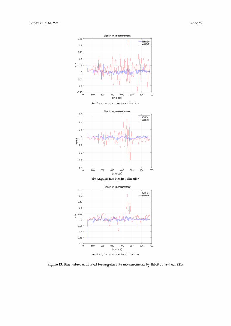
The bias estimations for the angular rate measurements showed a distinctive difference,and Figure 13 compares the estimated bias values. While the bias in the angular rate measurementfor the fixed wing UAV flight shows a difference in the average magnitude, as shown in Figure 6 ofSection 5.1, the bias in the quadrotor flight test shows a difference in the degree of fluctuation. The biasfor the ecl-EKF shows a larger fluctuation than that for the IEKF-av, as shown in Figure 13.

The Kalman gain and state error covariance most critically discriminate the IEKF-av from theecl-EKF. Only the Kalman gain is analyzed to save space. As shown in Figure 14, the IEKF-av has amore convergent Kalman gain, while that of the ecl-EKF exhibits periodic fluctuation, which dependson the attitude change in the quadrotor, like the results shown in Section 5.1.

Table 7 lists the results of a numerical analysis of the Kalman gain fluctuation. For all the Kalmangains except the Kalman gain Kbωy

with respect to zmy , the SM ratios for the IEKF-av are less thanthose for the ecl-EKF. Most of the Kalman gains for the IEKF-av are more convergent than those for theecl-EKF. This is the same feature as already revealed by Table 5 in Section 5.1.

Sensors 2018, 18, 2855 21 of 26

0 100 200 300 400 500 600 700

time(sec)

-20

-15

-10

-5

0

5

10

15

20

de

g

Roll

IEKF-av

ecl-EKF

(a) Estimated roll

0 100 200 300 400 500 600 700

time(sec)

-25

-20

-15

-10

-5

0

5

10

15

de

g

Pitch

IEKF-av

ecl-EKF

(b) Estimated pitch

0 100 200 300 400 500 600 700

time(sec)

-200

-150

-100

-50

0

50

100

150

200

de

g

Yaw

IEKF-av

ecl-EKF

(c) Estimated yaw

Figure 11. Attitudes estimated by IEKF-av and ecl-EKF for quadrotor flight test.

Sensors 2018, 18, 2855 22 of 26

0 100 200 300 400 500 600 700

time(sec)

-8

-6

-4

-2

0

2

4

6

m/s

Velocity North

IEKF-av

ecl-EKF

(a) Estimated x directional velocity

0 100 200 300 400 500 600 700

time(sec)

-5

-4

-3

-2

-1

0

1

2

3

4

5

m/s

Velocity East

IEKF-av

ecl-EKF

(b) Estimated y directional velocity

0 100 200 300 400 500 600 700

time(sec)

-3

-2.5

-2

-1.5

-1

-0.5

0

0.5

1

1.5

2

m/s

Velocity Down

IEKF-av

ecl-EKF

(c) Estimated z directional velocity

Figure 12. Velocities estimated by IEKF-av and ecl-EKF for quadrotor flight test.

Sensors 2018, 18, 2855 23 of 26

0 100 200 300 400 500 600 700

time(sec)

-0.15

-0.1

-0.05

0

0.05

0.1

0.15

0.2

0.25

rad

/s

Bias in wx measurement

IEKF-av

ecl-EKF

(a) Angular rate bias in x direction

0 100 200 300 400 500 600 700

time(sec)

-0.4

-0.3

-0.2

-0.1

0

0.1

0.2

0.3

rad

/s

Bias in wy measurement

IEKF-av

ecl-EKF

(b) Angular rate bias in y direction

0 100 200 300 400 500 600 700

time(sec)

-0.2

-0.15

-0.1

-0.05

0

0.05

0.1

0.15

0.2

0.25

rad

/s

Bias in wz measurement

IEKF-av

ecl-EKF

(c) Angular rate bias in z direction

Figure 13. Bias values estimated for angular rate measurements by IEKF-av and ecl-EKF.

Sensors 2018, 18, 2855 24 of 26

0 100 200 300 400 500 600 700

time(sec)

-8

-6

-4

-2

0

2

Kalm

an

ga

in

Kalman gain for qx correction

mx

my

mz

(a) Kalman gain of IEKF-av

0 100 200 300 400 500 600 700

time(sec)

-2

-1.5

-1

-0.5

0

0.5

1

1.5

2

2.5

Ka

lma

n g

ain

10-3 Kalman gain for q

x correction

mx

my

mz

(b) Kalman gain of ecl-EKF

Figure 14. Comparison of Kalman gain for correction of x-component of quaternion relative toinnovation of magnetic field measurements of IEKF-av and ecl-EKF.

Table 7. Comparison of Kalman gain for estimation of attitude and velocity in quadrotor flight test.

Kalman Gain ElementIEKF-av ecl-EKF

µ σ σ|µ| µ σ σ

|µ|

Kqx/zmx−0.0232 0.0127 0.5488 8.8141× 10−4 7.9180× 10−4 0.8983

Kqx/zmy−0.5474 0.0850 0.1553 1.7863× 10−4 0.0010 5.6959

Kqx/zmz−0.0911 0.0118 0.1296 6.3377× 10−4 5.4550× 10−4 0.8607

Kvz/zmx−0.0892 0.0157 1.6892 4.5189× 10−4 0.0020 4.4642

Kvz/zmy−0.0207 0.1250 6.0382 −4.3975× 10−4 0.0029 6.5964

Kvz/zmz0.0550 0.0931 1.6920 −2.6585× 10−4 0.0014 5.2806

Kbωy /zmx−0.5344 0.0508 0.0950 2.0447× 10−6 5.3013× 10−7 0.2593

Kbωy /zmy−0.0157 0.0413 2.6255 −2.2956× 10−7 4.2771× 10−7 1.8632

Kbωy /zmz0.3143 0.0290 0.0923 −3.4652× 10−7 1.3560× 10−6 3.9131

6. Conclusions

This paper evaluated the estimation performance and revealed the properties of the IEKF-basednavigation method through flight experiments with UAVs, and particularly through a comparison

Sensors 2018, 18, 2855 25 of 26

with the ecl-EKF, which is one of the prevalent navigation filters for small UAVs with limited sensormeasurements and computational capacity.

One of the distinctive features of the IEKF is its convergent Kalman gain, state error covariance,and estimation parameters such as measurement innovation and bias estimation. This is because thelinearized process model and measurement model of the IEKF depend only on invariant quantities,and the invariant quantities depend on the angular rate and acceleration. If the angular rate andacceleration are constant, the invariant quantities are constant, and thus the linearized model is constantand the filter converges to a linear Kalman filter. Even if the angular rate or acceleration changesinstantaneously, the Kalman gain and state error covariance converge again soon after the change.This property was verified in the Sections 5.1 and 5.2. Section 5.2 also demonstrated that, withoutlocation and altitude measurements, the IEKF was able to yield attitude and velocity estimations thatwere comparable to the estimations by the ecl-EKF for which location and altitude measurementswere utilized.

The IEKF can be derived using either the abstract Lie group methodology or matrix Lie groupmethodology [1,7]. This paper used the abstract Lie group-based derivation. For further research, it isrecommended to derive the matrix Lie group-based formulation of the IEKF for the same problemconsidered in this paper. In addition, it is expected that the problems addressed through the matrix Liegroup approach [7] can be solved by the abstract Lie group-based approach in the subsequent research.

Author Contributions: N.Y.K. conceived and developed the idea, designed and implemented the experiments,and coordinated the project that funded the estimations for unmanned vehicles. W.Y., I.H.C., G.S., and T.S.K.collaborated in the development of the idea, contributed to collecting measurement data, conducted the simulation,and performed revisions and improvements of the paper.

Funding: This work was funded by Institute for Information & Communications Technology Promotion (IITP),Ministry of Science and ICT (MSIT), Korea, No. 1711029259 (Technology Development of DMM-based ObstacleAvoidance and Vehicle Control System for a Small UAV) .

Conflicts of Interest: The authors declare no conflict of interest.

References

1. Barrau, A.; Bonnabel, S. Invariant Kalman Filtering. Annu. Rev. Control Robot. Auton. Syst. 2018, 1, 237–257.[CrossRef]

2. Martin, P.; Salaün, E. Generalized multiplicative extended Kalman filter for aided attitude and headingreference system. In Proceedings of the AIAA Guidance, Navigation, and Control Conference,Toronto, ON, Canada, 2–5 August 2010.

3. Lefferts, E.J.; Markley, F.L.; Shuster, M.D. Kalman filtering for spacecraft attitude estimation. J. Guid.Control Dyn. 1982, 5, 417–429. [CrossRef]

4. Markley, F.L. Attitude error representations for Kalman filtering. J. Guid. Control Dyn. 2003, 26, 311–317.[CrossRef]

5. Markley, F.L. Multiplicative vs. additive filtering for spacecraft attitude determination. Dyn. Control Syst.Struct. Space 2004. [CrossRef]

6. Bonnabel, S.; Martin, P.; Rouchon, P. Symmetry-preserving observers. IEEE Trans. Autom. Control 2008, 53,2514–2526. [CrossRef]

7. Barrau, A.; Bonnabel, S. The invariant extended Kalman filter as a stable observer. IEEE Trans. Autom. Control2017, 62, 1797–1812. [CrossRef]

8. Bonnable, S.; Martin, P.; Salaün, E. Invariant Extended Kalman Filter: Theory and application to avelocity-aided attitude estimation problem. In Proceedings of the 48th IEEE Conference on Decisionand Control Held Jointly with the 28th Chinese Control Conference (CDC/CCC 2009), Shanghai, China,15–18 December 2009.

9. Barrau, A.; Bonnabel, S. An EKF-SLAM algorithm with consistency properties. arXiv 2015, arXiv:1510.06263.10. Rouchon, P.; Rudolph, J. Invariant tracking and stabilization: Problem formulation and examples. In Stability

and Stabilization of Nonlinear Systems; Springer: London, UK, 1999; pp. 261–273.

Sensors 2018, 18, 2855 26 of 26

11. Aghannan, N.; Rouchon, P. On invariant asymptotic observers. In Proceedings of the 41st IEEE Conferenceon Decision and Control, Las Vegas, NV, USA, 10–13 December 2002.

12. Aghannan, N.; Rouchon, P. An intrinsic observer for a class of Lagrangian systems. IEEE Trans. Autom. Control2003, 48, 936–945. [CrossRef]

13. Martin, P.; Rouchon, P.; Rudolph, J. Invariant tracking. ESAIM Control Optim. Calc. Var. 2004, 10, 1–13.[CrossRef]

14. Bonnabel, S. Left-invariant extended Kalman filter and attitude estimation. In Proceedings of the 46th IEEEConference on Decision and Control, New Orleans, LA, USA, 12–14 December 2007.

15. Bonnabel, S.; Martin, P.; Rouchon, P. A nonlinear symmetry-preserving observer for velocity-aided inertialnavigation. In Proceedings of the American Control Conference, Minneapolis, MN, USA, 14–16 June 2006.

16. Barczyk, M. Nonlinear State Estimation and Modeling of a Helicopter UAV; University of Alberta:Edmonton, AB, Canada, 2012.

17. Tao, Z.; Bonnifait, P. Road invariant extended Kalman filter for an enhanced estimation of gps errors usinglane markings. In Proceedings of the 2015 IEEE/RSJ International Conference on Intelligent Robots andSystems (IROS), Hamburg, Germany, 28 September–2 October 2015.

18. Zhang, T.; Wu, K.; Song, J.; Huang, S.; Dissanayake, G. Convergence and consistency analysis for a 3-DInvariant-EKF SLAM. IEEE Robot. Autom. Lett. 2017, 2, 733–740. [CrossRef]

19. Barczyk, M.; Lynch, A.F. Invariant observer design for a helicopter UAV aided inertial navigation system.IEEE Trans. Control Syst. Technol. 2013, 21, 791–806. [CrossRef]

20. Barczyk, M.; Bonnabel, S.; Deschaud, J.E.; Goulette, F. Invariant EKF design for scan matching-aidedlocalization. IEEE Trans. Control Syst. Technol. 2015, 23, 2440–2448. [CrossRef]

21. Barczyk, M.; Lynch, A.F. Invariant extended Kalman filter design for a magnetometer-plus-GPS aided inertialnavigation system. In Proceedings of the 50th IEEE Conference on Decision and Control and EuropeanControl Conference (CDC-ECC), Orlando, FL, USA, 12–15 December 2011.

22. Pixhawk Overview. Available online: http://ardupilot.org/copter/docs/common-pixhawk-overview.html(accessed on 25 August 2018)

23. Px4 development guide. Available online: https://dev.px4.io/en/ (accessed on 25 August 2018).24. Output Predictor—Relationship to EKF. Available online: https://github.com/PX4/ecl/blob/master/EKF/

documentation/OutputPredictor.pdf (accessed on 25 August 2018).25. PX4/ecl. Available online: https://github.com/PX4/ecl/ (accessed on 25 August 2018).26. Using the ecl EKF. Available online: https://dev.px4.io/en/tutorials/tuning_the_ecl_ekf.html (accessed on

25 August 2018).

c© 2018 by the authors. Licensee MDPI, Basel, Switzerland. This article is an open accessarticle distributed under the terms and conditions of the Creative Commons Attribution(CC BY) license (http://creativecommons.org/licenses/by/4.0/).