ESTIMATING CORRELATIONS FROM A COASTAL OCEAN MODEL FOR LOCALIZING AN ENSEMBLE TRANSFORM KALMAN FILTER

Jonathan Poterjoy National Weather Center Research Experiences for Undergraduates, Norman, Oklahoma

Millersville University, Millersville, Pennsylvania

Ross N. Hoffman and Mark Leidner Atmospheric and Environmental Research, Inc., Lexington, Massachusetts

ABSTRACT

Data assimilation is the process of using past and present data to estimate the current

synoptic state of a dynamical system. Current data is merged with a previous model forecast or “background” field to produce the best estimate of a system’s state called an “analysis”. For cases where the probability distribution of observation and background errors are normally distributed, a Kalman filter can be shown to produce the best estimate of a variable and its uncertainty. A type of data assimilation system called the Ensemble Kalman Filter (EnKF) approximates the background covariance field using only a small ensemble of forecasts. Since a limited number of samples are used, many spurious correlations exist between an observation at one point and forecast errors at various locations within the model domain. To limit spurious relationships the Local Ensemble Transform Kalman filter (LETKF) limits the region considered in a process called “localization”. But a question arises regarding the optimal localization size for analyses within complex model domains. Using the Estuarine Coastal Ocean Model (ECOM) coupled with the LETKF, we examined correlations between simulated state variables on various locations and depths within a domain that spans the New York Harbor region. Distributions of correlation coefficients surrounding an analysis point were used to determine the optimal localization domain for each particular relationship. Since spurious correlations tend to diminish after 1 to 2 days of simulation, results observed during days 3 and 4 of this experiment were taken to be a good estimate of true relationships between variables. Given the large amount of dynamical and bathymetric variability within this model domain, correlation structures of mixed shapes and sizes were observed. In many instances, the parameterized localization domain was either too small or too large to capture the actual correlations. Results from this study provide incentive to pursue an automated solution to optimal localization within the LETKF/ECOM that tailors a unique localization volume for each analysis. If successful this solution can be applied to various other prediction systems that rely on ensemble data assimilation.

_________________________________________________________________ 1. Introduction

In situ and remotely sensed observations of large-scale geophysical systems, such as the earth’s atmosphere and oceans, tend to vary in density. Since it is not feasible to capture the true synoptic state of these systems at one instant (as required by forecast models), past and current observations are used in conjunction with a data assimilation system (DAS) for estimating the value of each state variable at all points in a specified model domain. At regular intervals, a DAS produces an “analysis” or statistical estimate of the system state at one moment in time. An analysis can be used to initialize a dynamical model to produce a “forecast” for future times, or empirically

to study the current synoptic situation. In both cases, data assimilation is a necessary step for understanding the nature of large complicated systems in cases where relatively few observations are available.

In terms of assimilating data for model initialization, the skill of any numerical prediction system depends on how efficiently observations are merged into the system. For cases where the model dynamics are linear in nature and where probability distributions of observation and forecast errors are normally distributed, a Kalman filter provided optimal estimates. Using current and past data, the Kalman filter uses the model dynamics to evolve the most probable trajectory of a system state and error (Kalman, 1960; Kalman

and Bucy, 1961). A previous model forecast or “background” is taken to be a good estimate or “first guess” for the current synoptic situation. An analysis is then created by minimizing a cost function with respect to a vector containing the system state. This function depends on the background vector, new observations, and error covariance matrices which represent the uncertainty for both of these vectors. The minimizing solution becomes the new analysis. A numerical model uses the current analysis to produce a forecast for the next time step, which is taken to be the new background field. The background error statistics are calculated and the data assimilation process is repeated with new observations and a new background. In general, the performance of any DAS depends on how well the current state vector and its error are estimated (Daley, 1991; Kalnay, 2002).

Since Kalman filtering is computationally expensive and only applies to dynamically linear systems, many variations of this DAS have been developed. One approach involves using an ensemble of analysis to produce a set of new forecasts (Evensen, 1994). For this case, the mean is taken to be the background; with an error covariance matrix approximated using the ensembles. Ott et al. (2004) and Hunt et al. (2007) describe the development of a portable, more efficient type of ensemble Kalman filter (EnKF) called the Local Ensemble Transform Kalman filter (LETKF) that nearly matches the EnKF in accuracy, but with a much improved run time.

Ensemble data assimilation provides a good way of determining the background error correlations. Since distant correlations are expected to be relatively insignificant, the LETKF limits the data region considered in a process called localization. That is only observations from a set localization volume are used (Ott et al., 2004).

Questions still remain concerning the localization size for state variables on each unique grid point: How strong is the relationship between the errors of a single variable estimation and all other variables at different points and levels throughout a model domain? How should the localization volume be tuned to best represent distinctive relationships?

To answer these questions, we ran a simulation experiment using the Estuarine Coastal Ocean Model (ECOM) coupled with the LETKF in the New York Harbor region. Results of this research suggest that large variability exists between state variable relationships throughout the model domain. Distributions of correlation

coefficients (r) between a single forecasted or analyzed point variable and the remaining field were used to represent such relationships. Overall, correlation structures tended to depend on variable, location, and time. To remove spurious correlations in remote locations, which can be regarded as noise, the results were averaged over various time spans.

This particular study is a small component of a much larger initiative to improve the accuracy and efficiency of the LETKF via better localization. The ultimate goal is to automate the process of localization within the ECOM/LETKF framework. In time, this method can be applied to other prediction systems that use ensemble-based DAS.

In Section 2, the methodology for this experiment is described. Details regarding the ECOM/LETKF domain are provided, along with the steps taken to examine state variable relationships and remove spurious correlations. The experiment results are explained in Section 3, including an overview of correlation structure variability with respect to variable, location and time. A summary and discussion on future research are provided in Sections 4 and 5.

2. Methodology

Originally developed for atmospheric

applications, the LETKF has been slightly modified for use in an oceanic environment with the Estuarine Coastal Ocean Model (for details see Hoffman et al., 2008). Previous improvements in modeling and data collection in the New York Harbor region have lead to the creation of the New York Harbor Observing and Prediction System (NYHOPS) (Blumberg et al. 1999; Bruno et al. 2006). Hoffman et al. (2008) have adapted the LETKF to work efficiently with the ECOM in the NYHOPS, proving it to be a useful test bed for advanced oceanic DA research. Using the same ECOM/LETKF configuration in the NYHOPS domain, we explored the localization component of the LETKF. a. Experiment Description

The ECOM/LETKF simulation was run for 4

days, producing 32 forecasts and analyses at 3 hour intervals. Most of the results we present from this study were obtained using an ensemble size (k) of 64, but for comparison we also examined results from an experiment that was run using k = 16. Water currents (u and v), salinity (S) and temperature (T) were predicted, along with surface water level (h). The current parameterization of the

Figure 1. Bathymetry (m) of NYHOPS domain in grid view, with all major geographic features labeled. LETKF localization volume is set at 2 horizontal grid lengths in both directions from the analysis point, and 1 to 2 grid lengths in the vertical.

The NYHOPS domain (Fig 1) has complex, irregular geometry including the New York Harbor and neighboring inland water features, such as the Hudson River, East River, Long Island Sound and Hudson Bight. The ECOM uses a 59x94 computational grid, with a resolution varying from 500 m in the rivers and estuaries to 42 km in the open ocean. Since bathymetry changes substantially throughout the

domain, the ECOM uses vertical !-coordinates

instead of z-coordinates, where ! is defined as the ratio between the depth and total height of a water column. Ten equally spaced levels are

used, ranging from ! = 0 at the water surface to

! = -1 at the ocean floor, with a vertical resolution that varies from about 150 m to less than 2 m, depending on bathymetry. b. Variable Relationships

The NYHOPS domain is ideal for this

particular type of study, where the relationships between variables at an assortment of locations in a diverse model domain are expected to vary substantially. To begin, each variable at selected locations is correlated with like variables at all grid points and levels in the model domain. A relationship is considered to be significant for |r|

> 0.6. An example of such a distribution is shown in Fig. 2a and 2b for the last time step of the simulation where the analysis ensemble correlations for S on point 45, 15, level 8 is illustrated. In this case for a location in the open ocean region, correlations are strong at grid points nearest to the site of interest and gradually taper off at distances further away. This occurrence is observed for most strong relationships. At the same location and depth, the analysis ensemble correlations for T are calculated (Fig. 2c and 2d) and a more compact horizontal correlation field is produced. In a similar manner, analysis ensemble correlations for u are shown in Fig. 2e and 2f with an even smaller distribution of significant correlations. A correlation structure for v-v relationships is not provided since it strongly resembles the distribution of u-u correlations at this location and depth. The grid point for these cases was chosen rather arbitrarily. What is important in this example is the fact that a significant difference in correlation structure exists for each variable at the same location and depth.

The above relationships were calculated for both ECOM analyses and backgrounds (forecasts) then subtracted for comparison. A large difference exists between the two distributions at several isolated locations for the first time step. Some of the values range from +/- 0.6 in regions where the correlation

NYHOPS Domain Bathymetry (m)

a b

c d

e f

Figure 2. The horizontal distribution of correlation between the point marked by ‘x’, and the remaining model domain are illustrated for S (a), T (c), and u (e) for the last time step of the simulation. Regions which are colored red represent large positive correlations, where blue shades indicate strong negative correlations and a white contour is plotted for |r| = 0.6. The area of interest for this case is at point 45, 15, level 8 in the NYHOPS domain; a location in the open ocean region off of the New York coast. To view the vertical correlation structure, cross sections are taken along the y-axis, extending from the coast to a location further out into the ocean, for S (b), T (d), and u (f).

coefficients are of moderate value. These differences quickly approach zero as the simulation is extended to more time steps. By the eighth time step (at the end of day 1) the two results have converged and a strong agreement exists between analysis and background correlations. c. Removing Spurious Correlations

To determine whether or not the observed

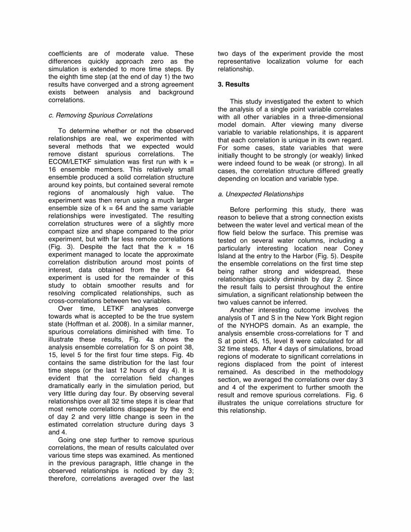
relationships are real, we experimented with several methods that we expected would remove distant spurious correlations. The ECOM/LETKF simulation was first run with k = 16 ensemble members. This relatively small ensemble produced a solid correlation structure around key points, but contained several remote regions of anomalously high value. The experiment was then rerun using a much larger ensemble size of k = 64 and the same variable relationships were investigated. The resulting correlation structures were of a slightly more compact size and shape compared to the prior experiment, but with far less remote correlations (Fig. 3). Despite the fact that the k = 16 experiment managed to locate the approximate correlation distribution around most points of interest, data obtained from the k = 64 experiment is used for the remainder of this study to obtain smoother results and for resolving complicated relationships, such as cross-correlations between two variables.

Over time, LETKF analyses converge towards what is accepted to be the true system state (Hoffman et al. 2008). In a similar manner, spurious correlations diminished with time. To illustrate these results, Fig. 4a shows the analysis ensemble correlation for S on point 38, 15, level 5 for the first four time steps. Fig. 4b contains the same distribution for the last four time steps (or the last 12 hours of day 4). It is evident that the correlation field changes dramatically early in the simulation period, but very little during day four. By observing several relationships over all 32 time steps it is clear that most remote correlations disappear by the end of day 2 and very little change is seen in the estimated correlation structure during days 3 and 4.

Going one step further to remove spurious correlations, the mean of results calculated over various time steps was examined. As mentioned in the previous paragraph, little change in the observed relationships is noticed by day 3; therefore, correlations averaged over the last

two days of the experiment provide the most representative localization volume for each relationship.

3. Results

This study investigated the extent to which

the analysis of a single point variable correlates with all other variables in a three-dimensional model domain. After viewing many diverse variable to variable relationships, it is apparent that each correlation is unique in its own regard. For some cases, state variables that were initially thought to be strongly (or weakly) linked were indeed found to be weak (or strong). In all cases, the correlation structure differed greatly depending on location and variable type. a. Unexpected Relationships

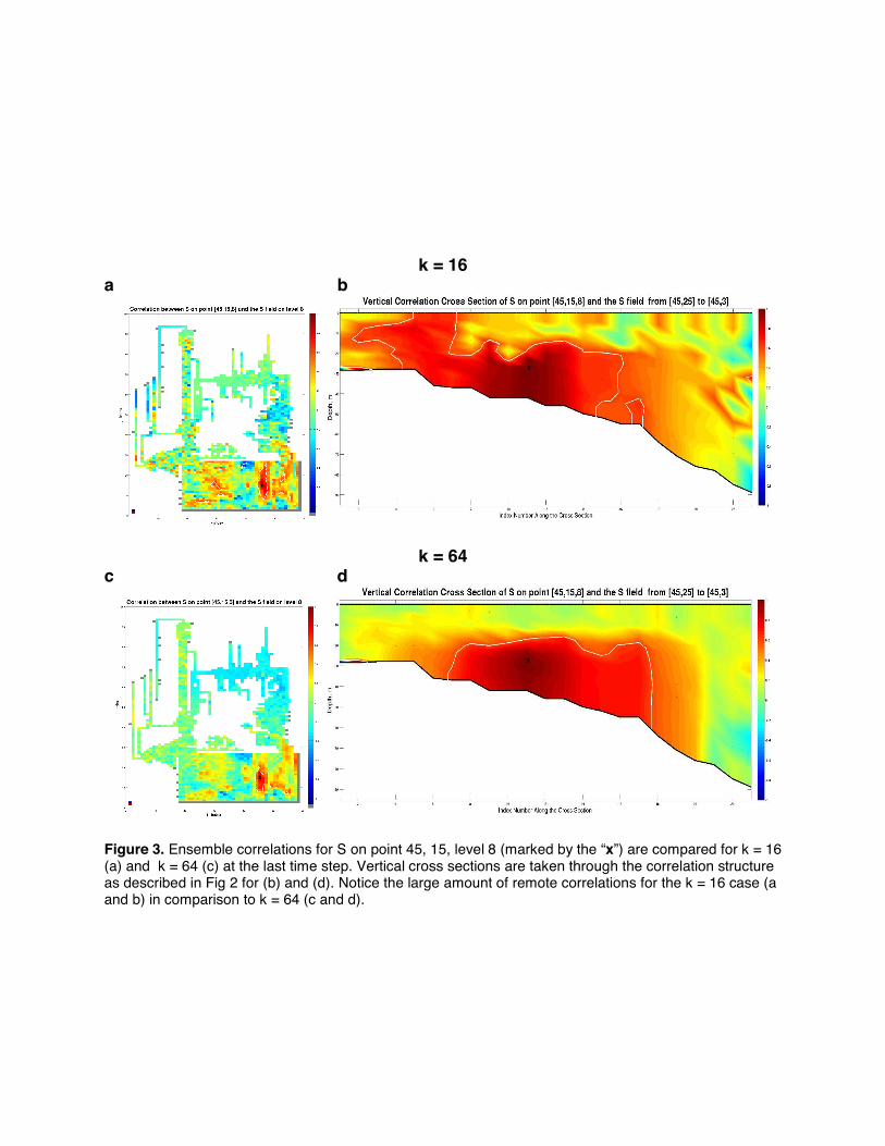
Before performing this study, there was reason to believe that a strong connection exists between the water level and vertical mean of the flow field below the surface. This premise was tested on several water columns, including a particularly interesting location near Coney Island at the entry to the Harbor (Fig. 5). Despite the ensemble correlations on the first time step being rather strong and widespread, these relationships quickly diminish by day 2. Since the result fails to persist throughout the entire simulation, a significant relationship between the two values cannot be inferred.

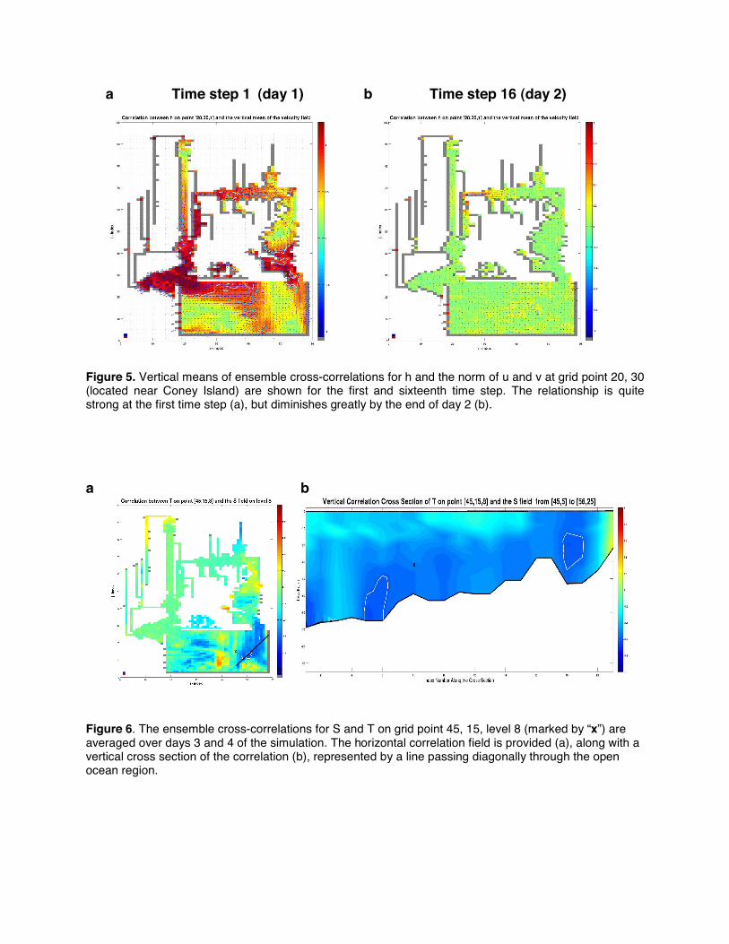
Another interesting outcome involves the analysis of T and S in the New York Bight region of the NYHOPS domain. As an example, the analysis ensemble cross-correlations for T and S at point 45, 15, level 8 were calculated for all 32 time steps. After 4 days of simulations, broad regions of moderate to significant correlations in regions displaced from the point of interest remained. As described in the methodology section, we averaged the correlations over day 3 and 4 of the experiment to further smooth the result and remove spurious correlations. Fig. 6 illustrates the unique correlations structure for this relationship.

k = 16

a b

k = 64 c d

Figure 3. Ensemble correlations for S on point 45, 15, level 8 (marked by the “x”) are compared for k = 16 (a) and k = 64 (c) at the last time step. Vertical cross sections are taken through the correlation structure as described in Fig 2 for (b) and (d). Notice the large amount of remote correlations for the k = 16 case (a and b) in comparison to k = 64 (c and d).

a

b

Figure 4. The evolution of a sample correlation field over time. For this example, ensemble correlations for S on grid point 38, 15, level 5 (marked by “x”) are illustrated. Correlations are shown for the first half of day 1 (a) and last half of day 4 (b). Notice how remote correlations quickly diminish after the first 4 time steps (a) and a persistent correlation structure emerges around the x by the end of the experiment (b).

a Time step 1 (day 1) b Time step 16 (day 2)

Figure 5. Vertical means of ensemble cross-correlations for h and the norm of u and v at grid point 20, 30 (located near Coney Island) are shown for the first and sixteenth time step. The relationship is quite strong at the first time step (a), but diminishes greatly by the end of day 2 (b).

a b

Figure 6. The ensemble cross-correlations for S and T on grid point 45, 15, level 8 (marked by “x”) are averaged over days 3 and 4 of the simulation. The horizontal correlation field is provided (a), along with a vertical cross section of the correlation (b), represented by a line passing diagonally through the open ocean region.

b. Potential for Improving Localization

The large amount of variability associated with correlation fields for like variables is the fundamental result of this study. For instance: significant T to T and S to S correlations tend to be more widespread than relationships involving components of current; therefore, a larger localization volume should be used. Likewise for water level: since significant h to h correlations cover an area that encompasses large fractions of the model domain (Fig. 7), a substantially larger localization region would be necessary to capture highly correlated observations.

Figure 7. An example horizontal ensemble correlation for h (marked by “x”) at point 25, 20 averaged over days 3 and 4 of the simulation.

The above relationships often differ greatly for various locations within the NYHOPS domain. Correlation structures associated with grid points located in the Hudson River tend to be relatively compact. For example, relationships involving u and v in this region diminish greatly by day 4 of the experiment –to the point where only correlations on the analysis point and one or two nearby grid points are significant. The dynamics of this region (i.e. shallow, fast moving water) is most likely what causes these relationships to fade. On the other side of the spectrum, correlations at points within small bay regions of the model domain are rather large.

Cross-correlations between variables are much more complicated. For nearly all regions

within the model domain, the analysis ensemble cross-correlations between T and S at an analysis point is quite minimal. When the same relationship is viewed for a point in vast open water regions such as the New York Bight, the cross-correlation structure is much larger and displaced slightly from the key analysis grid point (Fig. 6). The same phenomenon is present within the Long Island Sound and along coastal regions. 4. Summary Correlation coefficients were used in this experiment to study relationships between like and unlike variables within the NYHOPS domain. Many spurious correlations disappear by the end of day 2 for simulated results, providing good estimates of the true correlation structure at time steps during and after day 3. Results from the final two days of the experiment (days 3 and 4) were averaged to approximate the typical correlation structures associated with many relationships throughout the model domain. Values of |r| > 0.6 were taken to be significant. This criterion helped resolve the horizontal and vertical extent of the ideal localization volume for each relationship. These results shed light on the large amount of variability associated with analysis correlations in a diverse environment encompassing the New York Harbor and adjacent littoral regions. Surprising cross-correlations (or lack of correlation) were also discovered (Fig. 5 and 6). The current NYHOPS LETKF localization is set at 2 horizontal grid distances and 1 to 2 vertical levels, and appears to be deficient for many cases. The accuracy and efficiency of this prediction system can potentially be improved through larger localization volumes for variable analyses with strong relationships (S, T, h, and calm water regions), and smaller volumes for cases involving compact correlation structures (u, v, and highly variable flow regions). 5. Discussion Using disparate and noisy data, ensemble-based DAS perform very well for nonlinear dynamical systems such as the earth’s atmosphere or in this case an ocean system. Since Kalman filtering is too computationally expensive for operational use in large chaotic environments, solutions involving a localization

domain were developed (Ott et al. 2004; Hunt et al. 2007). This study is part of a much larger plan to improve localization within the LETKF/ECOM framework and possibly other prediction systems that use ensemble DAS. Results from this experiment reveal that parameterized localization volumes in current use inadequately represent the correlation structure for many variable relationships within the NYHOPS. Since we found a wide variability in correlation structures, it follows that the correct localization should also be variable. Throughout the course of this project, we found the optimal localization region for several state variable analyses on various locations within the NYHOPS domain. Improvements in the performance of this prediction system should result from an automated localization process; meaning more or less observations for individual analyses can be used, depending on correlation structure. If successful, this method can be applied to a variety of other applications, including non-traditional variables where correlation distributions are too complicated to resolve with set localization domains. Acknowledgements This material is based upon work supported by the National Science Foundation under Grant No. ATM-0648566. The first author would like to thank Sergey Vinogradov from AER for his assistance in generating the figures for this paper and Daphne Ladue for a wonderful REU experience. References

Blumberg, A. F., 1996: An estuarine and coastal ocean version of POM. Princeton Ocean Model Users Meeting, Princeton, NJ.

Blumberg, A. F., L. A. Khan, and J. P. St.

John, 1999: Three-dimensional hydrodynamic simulations of the New York Harbor, Long Island Sound and the New York Bight. J. Hydrologic Eng., 125, 799–816.

Bruno, M. S., A. F. Blumberg, and T. O.

Herrington, 2006: The urban ocean observatory – coastal ocean observations and forecasting in the New York Bight.

Journal of Marine Science and Environment, C4, 1–9.

Daley, R., 1991: Atmospheric Data Analysis. Cambridge University Press, 457 pp.

Evensen, G., 1994: Sequential data

assimilation with a nonlinear quasi-geostrophic model using Monte Carlo methods to forecast error statistics. J. Geophys. Res., 99 (C5), 10 143–10 162.

Kalman, R. 1960. A New approach to linear

filtering and prediction problems. Trans. ASME, Ser. D, J. Basic Eng. 82, 35-45

Kalman, R. and Bucy, R. 1961. New results in

linear filtering and prediction theory. Trans. ASME, Ser. D, J. Basic Eng. 83, 95-108.

Kalnay, E., 2002: Atmospheric Modeling, Data

Assimilation, and Predictability. Cambridge University Press, 364 pp.

Hoffman, R. N., R. M. Ponte, E. J. Kostelich, A.

Blumberg, I. Szunyogh, S. Vinogradov, and J. M. Henderson, “A simulation study using a local ensemble transform Kalman filter for data assimilation in New York Harbor,” J. Atoms. Oceanic Technol., 2008, In press.

Ott, E., B. R. Hunt, I. Szunyogh, A. V. Zimin, E.

J. Kostelich, M. Corazza, E. Kalnay, D. J. Patil, and J. A. Yorke, 2004: A local ensemble Kalman filter for atmospheric data assimilation. Tellus A, 56 (5), 415–428.