IEEE TRANSACTIONS ON SIGNAL PROCESSING 1

Distributing the Kalman Filter for

Large-Scale SystemsUsman A. Khan, Student Member, IEEE, Jose M. F. Moura, Fellow, IEEE

Department of Electrical and Computer Engineering

Carnegie Mellon University

5000 Forbes Ave, Pittsburgh, PA 15213

{ukhan, moura}@ece.cmu.edu

Ph: (412)268-7103 Fax: (412)268-3890

Abstract

This paper derives a distributed Kalman filter to estimate a sparsely connected, large-scale, n−dimensional, dy-

namical system monitored by a network of N sensors. Local Kalman filters are implemented on the (nl−dimensional,

where nl � n) sub-systems that are obtained after spatially decomposing the large-scale system. The resulting sub-

systems overlap, which along with an assimilation procedure on the local Kalman filters, preserve an Lth order

Gauss-Markovian structure of the centralized error processes. The information loss due to the Lth order Gauss-

Markovian approximation is controllable as it can be characterized by a divergence that decreases as L ↑. The order

of the approximation, L, leads to a lower bound on the dimension of the sub-systems, hence, providing a criterion for

sub-system selection. The assimilation procedure is carried out on the local error covariances with a distributed iterate

collapse inversion (DICI) algorithm that we introduce. The DICI algorithm computes the (approximated) centralized

Riccati and Lyapunov equations iteratively with only local communication and low-order computation. We fuse the

observations that are common among the local Kalman filters using bipartite fusion graphs and consensus averaging

algorithms. The proposed algorithm achieves full distribution of the Kalman filter that is coherent with the centralized

Kalman filter with an Lth order Gaussian-Markovian structure on the centralized error processes. Nowhere storage,

communication, or computation of n−dimensional vectors and matrices is needed; only nl � n dimensional vectors

and matrices are communicated or used in the computation at the sensors.

Index Terms

Large-scale systems, sparse matrices, distributed algorithms, matrix inversion, Kalman filtering, distributed esti-

mation, iterative methods

This work was partially supported by the DARPA DSO Advanced Computing and Mathematics Program Integrated Sensing and Processing

(ISP) Initiative under ARO grant # DAAD 19-02-1-0180, by NSF under grants # ECS-0225449 and # CNS-0428404, and by an IBM Faculty

Award.

November 23, 2009 DRAFT

arX

iv:0

708.

0242

v2 [

cs.I

T]

25

Feb

2008

IEEE TRANSACTIONS ON SIGNAL PROCESSING 2

I. INTRODUCTION

Centralized implementation of the Kalman filter [1], [2], although possibly optimal, does not provide robustness

and scalability when it comes to complex large-scale dynamical systems with their measurements distributed on a

large geographical region. The reasons are twofold: (i) the large-scale systems are very high-dimensional, and thus

extensive computations are required to implement the centralized procedure; and (ii) the span of the geographical

region, over which the large-scale system is deployed or the physical phenomenon is observed, poses a large

communication burden and thus, among other problems, adds latency to the estimation mechanism. To remove

the difficulties posed by the centralized procedure, we propose a distributed estimation algorithm with a low order

Kalman filter at each sensor. To account for the processing, communication, and limited resources at the sensors, the

local Kalman filters involve computations and communications with local quantities only, i.e., vectors and matrices

of low dimensions, nl � n, where n is the dimension of the state vector—no sensor computes, communicates, or

stores any n−dimensional quantity.

Much of the existing research on distributed Kalman filters focuses on sensor networks monitoring low di-

mensional systems, e.g., when multiple sensors mounted on a small number of robot platforms are used for

target tracking [3], [4], [5]. This scenario addresses the problem of how to efficiently incorporate the distributed

observations, which is also referred to in the literature as ‘data fusion,’ see also [6]. Data fusion for Kalman filters

over arbitrary communication networks is discussed in [7], using consensus protocols in [8]. References [9], [4]

incorporate packet losses, intermittent observations, and communication delays in the data fusion process. Although

these solutions work well for low-dimensional dynamical systems, e.g., target tracking applications, they implement

a replication of the n−dimensional Kalman filter at each sensor, hence, communicating and inverting n×n matrices

locally, which, in general, is an O(n3) operation. In contrast, in the problems we consider, the state dimension, n,

is very large, for example, in the range of 102 to 109, and so the nth order replication of the global dynamics in

the local Kalman filters is either not practical or not possible.

Kalman filters with reduced order models have been studied, in e.g., [10], [11] to address the computation burden

posed by implementing nth order models. In these works, the reduced models are decoupled, which is sub-optimal

as important coupling among the system variables is ignored. Furthermore, the network topology is either fully

connected [10], or is close to fully connected [11], requiring long distance communication that is expensive. We

are motivated by problems where the large-scale systems, although sparse, cannot be decoupled, and where, due

to the sensor constraints, the communication and computation should both be local. Multi-level systems theory to

derive a coordination algorithm among local Kalman filters is discussed in [12].

We present a distributed Kalman filter that addresses both the computation and communication challenges posed

by complex large-scale dynamical systems, while preserving its coupled structure; in particular, nowhere in our

distributed Kalman filter, do we require storage, communication, or computation of n−dimensional quantities. We

briefly explain the key steps and approximations in our solution.

Spatial Decomposition of Complex Large-Scale Systems: To distribute the Kalman filter, we provide a spatial

November 23, 2009 DRAFT

IEEE TRANSACTIONS ON SIGNAL PROCESSING 3

decomposition of the complex large-scale dynamical system (of dimension n) that we refer to as the overall system

into several, possibly many, local coupled dynamical systems (of dimension nl, such that nl � n) that we refer to

as sub-systems in the following. The large-scale systems, we consider, are sparse and localized. Physical systems

with such characteristics are described in section II-A. We exploit the underlying distributed and sparse structure

of system dynamics that results from a spatio-temporal discretization of random fields. Dynamical systems with

such structure are then spatially decomposed into sub-systems. The sub-systems overlap and thus the resulting local

Kalman filters also overlap. This overlap along with an assimilation procedure on the local error covariances (of the

local filters) preserve the structure of the centralized (approximated) error covariances. We preserve the coupling

by applying the coupled state variables as inputs to the sub-systems. In contrast, an estimation scheme using local

observers is addressed in [13], where the coupled states are also applied as inputs to the sub-systems, but, the

error covariances are not assimilated and remain decoupled. Such scheme loses its coherence with the centralized

procedure, as under arbitrary coupling, no structure of the centralized error covariance can be retained by the local

filters.

Overlapping Dynamics at the Sub-systems: Bipartite Fusion Graphs: The sub-systems that we extract from

the overall system overlap. This makes several state variables to be observed at different sub-systems. To fuse this

shared information, we implement a fusion algorithm using bipartite fusion graphs, which we introduced in [14],

and local average consensus algorithms [15], [8]. The interactions required by the fusion procedure are constrained

to a small neighborhood (this may require multi-hop communication in the small neighborhood). The multi-hop

communication requirements, in our case, arise because the dynamical field is distributed among local sub-systems

and only local processing is carried out throughout the development. In contrast, as noted earlier, a distributed

Kalman filter with single hop communication scheme is presented in [7], but, we reemphasize the fact the this

single-hop communications is a result of replicating nth order Kalman filters at each sensor.

Assimilation of the Local Error Covariances—Distributed Iterate-Collapse Inversion (DICI) Algorithm:

A key issue in distributing the Kalman filter is to maintain a reasonable coherence with the centralized estimation;

this is to say that the local error covariances should approximate the centralized error covariance in a well-defined

manner. If the local error covariances evolve independently at each sub-system they may lose any coherence with the

centralized error covariance under arbitrary coupling. To address this issue, we employ a cooperative assimilation

procedure among the local error covariances that preserves a Gauss-Markovian structure in the centralized error

processes. This is equivalent to approximating1 the inverse of the centralized error covariances (the information

matrices) to be L−banded2, as shown in [16]. The assimilation procedure is carried out with a distributed iterate-

collapse inversion (DICI, pronounced die-see) algorithm, briefly introduced in [17], that has an iterate step and a

collapse step.

1A measure on the loss of optimality is provided in section II-C and it will be shown that this measure serves as a criterion for choosing the

dimensions of the sub-systems.2We refer to a matrix as an L-banded matrix (L ≥ 0), if the elements outside the band defined by the Lth upper and Lth lower diagonal are 0.

November 23, 2009 DRAFT

IEEE TRANSACTIONS ON SIGNAL PROCESSING 4

We use the Information filter, [18], [11], format of the Kalman filter where the information matrices (inverse of

the error covariances) are iterated at each time step. We introduce the DICI algorithm that provides an iterative

matrix inversion procedure to obtain the local error covariances from the local information matrices. The inverses of

the local information matrices are assimilated among the sub-systems such that the local error covariances, obtained

after the assimilation, preserve the Gauss-Markovian structure of the centralized error covariances. Iterative matrix

inversion can also be carried out using the distributed Jacobi algorithm [19] where the computational complexity

scales linearly with the dimension, n, of the overall system. In contrast, the computational complexity of the DICI

algorithms is independent of n. In addition, the error process of the DICI algorithm is bounded above by the error

process of the distributed Jacobi algorithm. We show the convergence of the iterate step of the DICI algorithm

analytically and resort to numerical simulations to show the convergence of its collapse step.

In summary, the spatial decomposition of the complex large-scale systems, fusion algorithms for fusing observa-

tions, the DICI algorithm to assimilate the local error covariance combine to give a robust, scalable, and distributed

implementation of the Kalman filter.

We describe the rest of the paper. Section II covers the discrete-time models, centralized Information filters, and

centralized L−banded Information filters. Section III covers the model distribution step. We introduce the local

Information filters in section III-B along with the necessary notation. Section IV gives the observation fusion step of

the local Information filters, and section V presents the distributed iterate collapse inversion (DICI) algorithm. The

filter step of the local Information filters is provided in section VI, and the prediction step of the local Information

filters is provided in section VII. We conclude the paper with results in section VIII and conclusions in section IX.

Appendix I discusses the L−banded inversion theorem, [20].

II. BACKGROUND

In this section, we motivate the type of applications and large-scale dynamical systems of interest to us. The

context is that of a time-varying random field governed by partial differential equations (PDEs); these systems can

also be generalized to arbitrary dynamical systems belonging to a particular structural class, as we elaborate in

Subsection II-A. To fix notation, we then present the centralized version of the Information filter.

A. Global Model

Many physical phenomenon [21], [22], [23], [24], [25], [26], e.g., ocean/wind circulation and heat/wave equations,

can be broadly characterized by a PDE of the Navier-Stokes type. These are highly non-linear and different regimens

arise from different assumptions. Non-linear approximation models are commonly used for prediction (predictive

models). For data assimilation, i.e., combining models with measured data, e.g., satellite altimetry data in ocean

models, it is unfeasible to use non-linear models; rather linearized approximations (dynamical linearization) are

employed. Here, our goal is to motivate how discrete linear models occur that exhibit a sparse and localized

structure that we use to distribute the model in Section III. Hence, we take a very simplistic example and consider

November 23, 2009 DRAFT

IEEE TRANSACTIONS ON SIGNAL PROCESSING 5

elliptical operators, given by,

L = α∂2

∂ρ2x

+ β∂2

∂ρ2y

, (1)

where ρx and ρy represent the horizontal and vertical dimensions, respectively, and α, β are constants pertinent

to the specific application. The spatial model for the continuous-time physical phenomenon (e.g., heat, wave, or,

wind), xt, with a continuous-time random noise term, ut, can now be written as,

Lxt = ut, (2)

which reduces to a Laplacian equation, ∆xt = 0 (∆ = ∂2/∂ρ2x + ∂2/∂ρ2

y), or to a Poisson equation, −∆xt = ut,

for appropriate choices of the constants. We spatially discretize the general model in (2) on an M × J uniform

mesh grid, where the standard 2nd order difference equation approximation to the 2nd order derivative is

∂2xt∂ρ2

x

∼ xi+1,j − 2xi,j + xi−1,j ,∂2xt∂ρ2

y

∼ xi,j+1 − 2xi,j + xi,j−1, (3)

where xij is the value of the random field, xt, at the ij-th location in the M × J grid. With this approximation,

the Laplace equation (say), leads to the individual equations of the form

xi,j −14

(xi,j−1 + xi,j+1 + xi−1,j + xi+1,j) = 0. (4)

Let I be an identity matrix and let A be a tridiagonal matrix with zeros on the main diagonal and ones on the

upper and lower diagonals, then (4), ∀ i, j ∈M ×J (with appropriate constants for modeling the elliptical operator

in (2)), can be collected in the linear system of equations and (2) can be spatially discretized in the form

Fcxt = bc + Gcut, (5)

where the vector bc collects the boundary conditions, the term Gcut controls where the random noise is added and

xt =[(

x1t

)T, . . . ,

(xMt)T ]T

(6)

and xit = [xi1, . . . , xiJ ]T . The matrix Fc is given by

Fc =

B C. . . . . . . . .

C B

= I⊗B + A⊗C, (7)

where B = µI + βhA, and C = βvI, the constants µ, βh, βv are in terms of α, β in (1), and ⊗ is the Kronecker

product [27].

If we further include time dependence, e.g., by discretizing the diffusion equation, we get

xt = Fcxt − bc −Gcut, (8)

where xt = dxt/dt. We again employ the standard first difference approximation of the first derivative with 4Tbeing the sampling interval and k being the discrete-time index, and, write the above equation as

xk+1 = (I +4TFc) xk −4Tbc −4TGcuk, k ≥ 0 (9)

November 23, 2009 DRAFT

IEEE TRANSACTIONS ON SIGNAL PROCESSING 6

which can be generalized as the following discrete-time model (where for simplicity of the presentation and without

loss of generality we drop the term bc in the sequel)

xk+1 = Fxk + Guk. (10)

In the above model, xk ∈ Rn is the state vector, x0 ∈ Rn are the initial state conditions, F ∈ Rn×n is the model

matrix, uk ∈ Rj′ is the state noise vector and G ∈ Rn×j′ is the state noise matrix.

Here, we note that the model matrix, F, is is perfectly banded in case of PDEs as in (7). We can relax this to

sparse and localized, i.e., the coupling among the states decays with distance (in an appropriate measure). Besides

random fields, the discrete-space-time model (10) with sparse and localized structure also occurs, e.g., in image

processing, the dynamics at a pixel depends on neighboring pixel values [28], [29]; in power systems, the power

grid models, under certain assumptions, exhibit banded structures, [30], [31], [32]. Systems that are sparse but not

localized can be converted to sparse and localized by using matrix bandwidth reduction algorithms [33]. We further

assume that the overall system is coupled, irreducible, and globally observable.

Let the system described in (10) be monitored by a network of N sensors. Observations at sensor l and time k are

y(l)k = Hlxk + w(l)

k , (11)

where Hl ∈ Rpl×n is the local observation matrix for sensor l, pl is the number of simultaneous observations made

by sensor l at time k, and w(l)k ∈ Rpl is the local observation noise. In the context of the systems we are interested

in, it is natural to assume that the observations are localized. These local observations at sensor l may be, e.g., the

temperature or height at location l or an average of the temperatures or heights at l and neighboring locations.

We stack the observations at all N sensors in the sensor network to get the global observation model as follows.

Let p be the total number of observations at all the sensors. Let the global observation vector, yk ∈ Rp, the global

observation matrix, H ∈ Rp×n, and the global observation noise vector, wk ∈ Rp, be

yk =

y(1)k

...

y(N)k

, H =

H1

...

HN

, wk =

w(1)k

...

w(N)k

. (12)

Then the global observation model is given by

yk = Hxk + wk. (13)

We adopt standard assumptions on the statistical characteristics of the noise. The state noise sequence, {uk}k≥0,

the observation noise sequence, {wk}k≥0, and the initial conditions, x0, are independent, Gaussian, zero-mean, with

E[uιuHτ ] = Qδιτ and E[wιwHτ ] = Rδιτ , and E[x0xH0 ] = S0, (14)

where the superscript H denotes the Hermitian, the Kronecker delta διτ = 1, if and only if ι = τ , and zero

otherwise. Since the observation noise at different sensors is independent, we can partition the global observation

noise covariance matrix, R, with Rl ∈ Rpl×pl being the local observation noise covariance matrix at sensor l, as

R = blockdiag[R1, . . . ,RN ]. (15)

November 23, 2009 DRAFT

IEEE TRANSACTIONS ON SIGNAL PROCESSING 7

For the rest of the presentation, we consider time-invariant models, specifically, the matrices, F,G,H,Q,R, are

time-invariant. The discussion, however, is not limited to either zero-mean initial condition or time-invariant models

and generalizations to the time-variant models will be added as we proceed.

B. Centralized Information Filter

Let Sk|k and Sk|k−1 be (filtered and prediction) error covariances, and their inverses be the information matri-

ces, Zk|k and Zk|k−1. Let xk|k and xk|k−1 be the filtered estimate and the predicted estimate of the state vector, xk,

respectively. We have the following relations.

Sk|k = Z−1k|k (16)

Sk|k−1 = Z−1k|k−1 (17)

zk|k−1 = Zk|k−1xk|k−1 (18)

zk|k = Zk|kxk|k (19)

Define the n−dimensional global observation variables as

ik = HTR−1yk, (20)

I = HTR−1H, (21)

and the n−dimensional local observation variables at sensor l as

il,k = HTl R−1

l y(l)k , (22)

Il = HTl R−1

l Hl. (23)

When the observations are distributed among the sensors, see (11), the CIF can be implemented by collecting all

the sensor observations at a central location; or with observation fusion by realizing that the global observation

variables in (20)−(21), can be written as, see [3], [11], [7],

ik = HTR−1yk

= HT1 R−1

1 y(1)k + · · ·+ HT

NR−1N y(N)

k

=N∑l=1

il,k. (24)

Similarly,

I =N∑l=1

Il. (25)

The filter step of the CIF is

Zk|k = Zk|k−1 +N∑l=1

Il, k ≥ 0 (26a)

zk|k = zk|k−1 +N∑l=1

il,k, k ≥ 0. (26b)

November 23, 2009 DRAFT

IEEE TRANSACTIONS ON SIGNAL PROCESSING 8

The prediction step of the CIF is

Zk|k−1 = S−1k|k−1 = (FZ−1

k−1|k−1FT+GQGT )−1

, k ≥ 1, Z0|−1 = S−10 , (27a)

zk|k−1 = Zk|k−1

(FZ−1

k−1|k−1zk−1|k−1

), k ≥ 1, z0|−1 = 0. (27b)

C. Centralized L−Banded Information filters

To avoid the O(n3) computations of the global quantities in (27), e.g., the inversion, Z−1k−1|k−1, we approximate

the information matrices, Zk|k and Zk|k−1, to be L−banded matrices, Zk|k and Zk|k−1. We refer to the CIF with

this approximation as the centralized L−banded Information filter (CLBIF). This approach is studied in [34], where

the information loss between Z and Z, is given by the divergence (see [34])

Divergence(Z,Z) =12

∣∣∣∣∣∣Z−T2

(Z− Z

)Z−

12

∣∣∣∣∣∣2F≤ 1

2

(∑i

λ− 1

2i(Z)

)2(∑i

λ− 1

2

i(Z)

)2 ∣∣∣∣∣∣Z− Z∣∣∣∣∣∣2F, (28)

where || · ||F is the Frobenius norm and λi(Z) is the ith eigenvalue of the matrix Z.

This approximation on the information matrices is equivalent to approximating the Gaussian error processes,

εk|k = xk − xk|k, εk|k−1 = xk − xk|k−1, (29)

to be Gauss-Markovian of Lth order [16]. Reference [20] presents an algorithm to derive the approximation that is

optimal in Kullback-Leibler or maximum entropy sense in the class of all L−banded matrices approximating the

inverse of the error covariance matrix. In the sequel, we assume this optimal L−banded approximation.

The CLBIF (with the L−banded information matrices, Zk|k and Zk|k−1) is given by the filter step in (26a)−(26b)

and the prediction step in (27a)−(27b), where the optimal information matrices, Zk|k and Zk|k−1, are replaced by

their L−banded approximations. The algorithms in [20], [35] reduce the computational complexity of the CLBIF

to O(n2) but the resulting algorithm is still centralized and deals with the n−dimensional state. To distribute the

CLBIF, we start by distributing the global model (10)−(13) in the following section.

III. SPATIAL DECOMPOSITION OF COMPLEX LARGE-SCALE SYSTEMS

Instead of implementing CLBIF based on the global model, we implement local Information filters at the sub-

systems obtained by spatially decomposing the overall system. Subsection III-A deals with this decomposition by

exploiting the sparse and localized structure of the model matrix, F. In the following, we devise a sub-system at

each sensor monitoring the system. This can be applied to general model matrices, F, but is only practical if F is

sparse and localized as we explain below.

A. Reduced Models at Each Sensor

This subsection shows how to distribute the global model (10) and (13), in order to get the reduced order sub-

systems. We illustrate the procedure with a simple example that reflects our assumptions on the dynamical system

November 23, 2009 DRAFT

IEEE TRANSACTIONS ON SIGNAL PROCESSING 9

structure. Consider a five dimensional system with the global dynamical model

xk+1 =

f11 f12 0 0 0

f21 f22 0 f24 0

f31 0 f33 0 0

0 0 f43 0 f45

0 0 0 f54 f55

xk +

0 0

0 0

0 g32

0 0

g51 0

uk (30)

= Fxk + Guk.

The system has two external noise sources uk = [u1k, u2k]T . We monitor this system with N = 3 sensors, having

scalar observations, y(l)k , at each sensor l. The global observation vector, yk, stacks the local observations, y(l)

k , and is

yk =

y

(1)k

y(2)k

y(3)k

=

1 1 1 0 0

0 1 1 1 0

0 0 0 1 1

xk +

w

(1)k

w(2)k

w(3)k

(31)

= Hxk + wk,

where H = [HT1 HT

2 HT3 ]T . We distribute global model of equations (30) and (31) in the following Subsections.

1) Graphical Representation using System Digraphs: A system digraph visualizes the dynamical interdependence

of the system. A system digraph, [13], J = [V,E], is a directed graphical representation of the system, where V =

X ∪ U is the vertex set consisting of the states, X = {xi}i=1,...,n, and the noise inputs, U = {ui}i=1,...,j . The

interconnection matrix, E, is the binary representation (having a 1 for each non-zero entry) of the model matrix, F,

and the state noise matrix, G, concatenated together. The interconnection matrix, E, for the system in (30) is,

E =

1 1 0 0 0 0 0

1 1 0 1 0 0 0

1 0 1 0 0 0 1

0 0 1 0 1 0 0

0 0 0 1 1 1 0

. (32)

The system digraph is shown in Figure 1(a).

2) Reduced Models from the Cut-point Sets: We have N = 3 sensors monitoring the system through the

observation model (31). We associate to each sensor l a cut-point set, V (l), where V (l) ⊆ X . If a sensor observes

a linear combination of several states, its cut-point set, V (l), includes all these states; see [36] for the definition of

cut-point sets, and algorithms to find all cut-point sets and a minimal cut-point set, if it exists. The cut-point sets

select the local states involved in the local dynamics at each sensor. From (31), the cut-point sets3 are shown in

3For simplicity of the presentation, we chose here that each state variable is observed by at least one sensor. If this is not true, we can easily

account for this by extending the cut-point sets, V (l), to V (l), such that

N[l=1

V(l)

= X. (33)

November 23, 2009 DRAFT

IEEE TRANSACTIONS ON SIGNAL PROCESSING 10

x4

x2

x1

x3

x5

u2

u1

(a)

x4

x2

x1

x3

x5

u2

u1

s1

s2

s3

(b)

Fig. 1. System Digraph and cut-point sets: (a) Digraph representation of the 5 dimensional system, (30)−(31). The circles represent the

states, x, and the squares represent the input noise sources, u. (b) The cut-point sets associated to the 3 sensors (4) are shown by the dashed

circles.

F(1) D(1)

f11 f12 0 0 0f21 f22 0 f24 0f31 0 f33 0 00 0 f43 0 f45

0 0 0 f54 f55

F1

F(3)D(3)

F3

Fig. 2. Partitioning of the global model matrix, F, into local model matrices, F(l), and the local internal input matrices, D(l), shown for

sensor 1 and sensor 3, from the example system, (30)−(31).

Figure ?? where we have the following cut-point set, e.g., at sensor 1,

V (1) = {x1, x2, x3} . (34)

Dimension of the sub-systems: The local states at sensor l, i.e., the components of the local state vector, x(l)k ,

are the elements in its associated cut-point set, V (l). The dimension of the local Kalman filter implemented at sensor

l is now nl. The set of nl-dimensional local Kalman filters will give rise, as will be clear later, to an L-banded

centralized Information matrix with L = min(n1, . . . , nN ). The loss in the optimality as a function of L is given by

the divergence (28). Hence, for a desired level of performance, i.e., for a fixed L, we may need to extend (include

additional states in a cut-point set) the cut-point sets, V (l), to V (l)L , such that

nl =∣∣∣V (l)L

∣∣∣ ≥ L, ∀ l, (35)

where | · | when applied to a set denotes its cardinality. This procedure of choosing an L based on a certain desired

performance gives a lower bound on the dimensions of the sub-systems.

November 23, 2009 DRAFT

IEEE TRANSACTIONS ON SIGNAL PROCESSING 11

Coupled States as Inputs: The directed edges coming into a cut-point set are the inputs required by the reduced

model. In the context of our running illustration (30)−(31), we see that the local state vector for sensor 1 is, x(1)k =

[x1,k, x2,k, x3,k]T , and the inputs to the local model consist of a subset of the state set, X , (at sensor s1, x4,k is

the input coming from sensor s2) and a subset of the noise input set, U , (u2,k at sensor s1).

Local models: For the local model at sensor l, we collect the states required as input in a local internal input

vector, d(l)k (we use the word internal to distinguish from the externally applied inputs), and the noise sources

required as input in a local noise input vector, u(l)k . We collect the elements from F corresponding to the local

state vector, x(l)k , in a local model matrix, F(l). Similarly, we collect the elements from F corresponding to the

local internal input vector, d(l)k , in a local internal input matrix, D(l), and the elements from G corresponding to

the local noise input vector, u(l)k , in a local state noise matrix, G(l). Figure 2 shows this partitioning for sensors s1

and s3. We have the following local models for (30).

x(1)k+1 =

f11 f12 0

f21 f22 0

f31 0 f33

x(1)k +

0

f24

0

x4,k +

0

0

g32

u2,k,

= F(1)x(1)k + D(1)d(1)

k + G(1)u(1)k (36)

x(2)k+1 =

f22 0 f42

0 f33 0

0 f43 0

x(2)k +

f21 0

f31 0

0 f45

x1,k

x5,k

+

0

g32

0

u2,k,

= F(2)x(2)k + D(2)d(2)

k + G(2)u(2)k (37)

x(3)k+1 =

0 f45

f54 f55

x(3)k +

f43

0

x3,k +

0

g51

u1,k,

= F(3)x(3)k + D(3)d(3)

k + G(3)u(3)k (38)

We may also capture the above extraction of the local states by the cut-point sets, with the following procedure.

Let the total number of states in the cut-point set at sensor l, V (l), be nl. Let Tl be an nl × n selection matrix,

such that it selects nl states in the cut-point set, V (l), from the entire state vector, xk, according to the following

relation,

x(l)k = Tlxk. (39)

For sensor 1, the selection matrix, T1, is

T1 =

1 0 0 0 0

0 1 0 0 0

0 0 1 0 0

. (40)

November 23, 2009 DRAFT

IEEE TRANSACTIONS ON SIGNAL PROCESSING 12

InitializeVI-A

Observation FusionIV-A

Local Filter StepVI-B

Distributed Matrix Inversion using DICI

V

Local Prediction Step

VII

Fig. 3. Block Diagram for the LIFs: Steps involved in the LIF implementation. The ovals represent the steps that require local communication.

We establish a reduced local observation matrix, H(l), by retaining the terms corresponding to the local state

vector, x(l)k , from the local observation matrix, Hl. We may write

H(l) = HlT#l , (41)

where ‘#’ denotes the pseudo-inverse of the matrix. In the context of the running illustration, the reduced local

observation matrix H(1) = [1, 1, 1] is obtained from the local observation matrix H1 = [1, 1, 1, 0, 0]. Note that Hl

picks the states from the global state vector, xk, whereas H(l) picks the states from the local state vector, x(l)k . The

reduced local observation models are given by

y(l)k = H(l)x(l)

k + w(l)k . (42)

We now make some additional comments. For simplicity of the explanation, we refer to our running exam-

ple, (30)−(31). We note that the reduced models at the sensors overlap, as shown by the overlapping cut-point

sets in Figure ??. Due to this overlap, observations corresponding to the shared states are available at multiple

sensors that should be fused. We further note that the reduced model (36) at sensor 1 is coupled to the reduced

model (37) at sensor 2 through the state x4,k. The state x4,k at sensor 1 does not appear in the local state vector,

i.e., x4,k /∈ x(1)k . But it is still required as an internal input at sensor 1 to preserve the global dynamics. Hence,

sensor 2 communicates the state x4,k, which appears in its local state vector, i.e., x4,k ∈ x(2)k , to sensor 1. Hence

at an arbitrary sensor l, we derive the reduced model to be

x(l)k+1 = F(l)x(l)

k + D(l)d(l)k + G(l)u(l)

k . (43)

Since the value of the state itself is unknown, sensor 2 communicates its estimate, x(2)4,k|k, to sensor 1. This allows

sensor 1 to complete its local model and preserve global dynamics, thus, taking into account the coupling between

the local reduced-order models. This process is repeated at all sensors. Hence, the local internal input vector, d(l)k ,

is replaced by its estimate, d(l)k|k. It is worth mentioning here that if the dynamics were time-dependent, i.e., the

matrices, F,G,H, change with time, k, then the above decomposition procedure will have to be repeated at each k.

This may result into a different communication topology over which the sensors communicate at each k.

November 23, 2009 DRAFT

IEEE TRANSACTIONS ON SIGNAL PROCESSING 13

s11 s12 s13 s14 s15

s12 s22 s23 s24 s25

s13 s23 s33 s34 s35

s14 s24 s34 s44 s45

s15 s25 s35 s45 s55

z11 z12 0z12 z22 z23

z23 z33 z34

z34 z44 z45

0 z45 z55

-1

-1== =

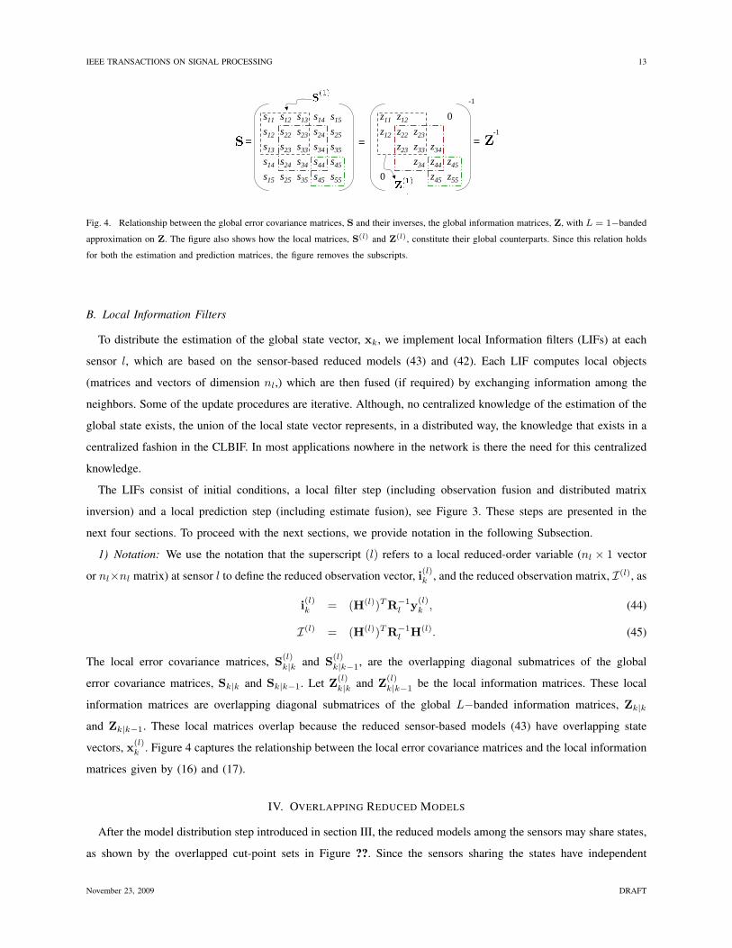
Fig. 4. Relationship between the global error covariance matrices, S and their inverses, the global information matrices, Z, with L = 1−banded

approximation on Z. The figure also shows how the local matrices, S(l) and Z(l), constitute their global counterparts. Since this relation holds

for both the estimation and prediction matrices, the figure removes the subscripts.

B. Local Information Filters

To distribute the estimation of the global state vector, xk, we implement local Information filters (LIFs) at each

sensor l, which are based on the sensor-based reduced models (43) and (42). Each LIF computes local objects

(matrices and vectors of dimension nl,) which are then fused (if required) by exchanging information among the

neighbors. Some of the update procedures are iterative. Although, no centralized knowledge of the estimation of the

global state exists, the union of the local state vector represents, in a distributed way, the knowledge that exists in a

centralized fashion in the CLBIF. In most applications nowhere in the network is there the need for this centralized

knowledge.

The LIFs consist of initial conditions, a local filter step (including observation fusion and distributed matrix

inversion) and a local prediction step (including estimate fusion), see Figure 3. These steps are presented in the

next four sections. To proceed with the next sections, we provide notation in the following Subsection.

1) Notation: We use the notation that the superscript (l) refers to a local reduced-order variable (nl × 1 vector

or nl×nl matrix) at sensor l to define the reduced observation vector, i(l)k , and the reduced observation matrix, I(l), as

i(l)k = (H(l))TR−1l y(l)

k , (44)

I(l) = (H(l))TR−1l H(l). (45)

The local error covariance matrices, S(l)k|k and S(l)

k|k−1, are the overlapping diagonal submatrices of the global

error covariance matrices, Sk|k and Sk|k−1. Let Z(l)k|k and Z(l)

k|k−1 be the local information matrices. These local

information matrices are overlapping diagonal submatrices of the global L−banded information matrices, Zk|k

and Zk|k−1. These local matrices overlap because the reduced sensor-based models (43) have overlapping state

vectors, x(l)k . Figure 4 captures the relationship between the local error covariance matrices and the local information

matrices given by (16) and (17).

IV. OVERLAPPING REDUCED MODELS

After the model distribution step introduced in section III, the reduced models among the sensors may share states,

as shown by the overlapped cut-point sets in Figure ??. Since the sensors sharing the states have independent

November 23, 2009 DRAFT

IEEE TRANSACTIONS ON SIGNAL PROCESSING 14

x1 x5x4x3x2

s3s2s1

Fig. 5. Bipartite Fusion graph, B, is shown for the example system, (30)−(31).

observations of the shared states, observations corresponding to the shared states should be fused. We present

observation fusion in subsection IV-A with the help of bipartite fusion graphs, [14].

A. Observation Fusion

Equations (24) and (25) show that the observation fusion is equivalent to adding the corresponding n−dimensional

local observation variables, (22)−(23). In CLBIF, we implement this fusion directly because each local observation

variable in (22)−(23) corresponds to the full n−dimensional state vector, xk. Since the nl−dimensional reduced

observation variables, (44)−(45), correspond to different local state vectors, x(l)k , they cannot be added directly.

To achieve observation fusion, we introduce the following undirected bipartite fusion graph4, B. Let SN =

{s1, . . . , sN} be the set of sensors and X be the set of states. The vertex set of the bipartite fusion graph, B,

is SN⋃X . We now define the edge set, EB, of the fusion graph, B. The sensor si is connected to the state

variable xj , if si observes the state variable xj . In other words, we have an edge between sensor si and state

variable xj , if the local observation matrix, Hi, at sensor si, contains a non-zero entry in its jth column. Figure 5

shows the bipartite graph for the example system in (30)−(31).

We now further provide some notation on the communication topology. Let G denote the sensor communication

graph that determines how the sensors communicate among themselves. Let K(l) be the subgraph of G, that contains

the sensor l and the sensors directly connected to the sensor l. For the jth state, xj , let Gj be the induced subgraph

of the sensor communication graph, G, such that it contains the sensors having the state xj in their reduced models.

The set of vertices in Gj come directly form the bipartite fusion graph, B. For example, from Figure 5, we

see that G1 contains s1 as a single vertex, G2 contains s1, s2 as vertices, and so on. States having more than one

sensor connected to them in the bipartite fusion graph, B, are the states for which fusion is required, since we have

multiple observations for that state. Furthermore, Figure 5 also gives the vertices in the associated subgraphs, Gj ,

over which the fusion is to be carried out.

With the help of the above discussion, we establish the fusion of the reduced observation variables, (44)−(45).

The reduced model at each sensor involves nl state variables, and each element in the nl × 1 reduced observation

vector, i(l)k , corresponds to one of these states, i.e., each entry in i(l)k has some information about its corresponding

4A bipartite graph is a graph whose vertices can be divided into two disjoint sets X and SN , such that, every edge connects a vertex in X

to a vertex in SN , and, there is no edge between any two vertices of the same set, [37].

November 23, 2009 DRAFT

IEEE TRANSACTIONS ON SIGNAL PROCESSING 15

state variable. Let the entries of the nl × 1 reduced observation vector, i(l)k , at sensor l, be subscripted by the nl

state variables modeled at sensor l. In the context of the example given by system (30)−(31), we have

i(1)k =

i(1)k,x1

i(1)k,x2

i(1)k,x3

, i(2)k =

i(2)k,x2

i(2)k,x3

i(2)k,x4

, i(3)k =

i(3)k,x4

i(3)k,x5

. (46)

For each state xj , the observation fusion is carried out on the sensors attached to this state in the bipartite fusion

graph, B. The fused observation vectors denoted by i(l)f,k are given by

i(1)f,k =

i(1)k,x1

i(1)k,x2

+ i(2)k,x2

i(1)k,x3

+ i(2)k,x3

, i(2)f,k =

i(2)k,x2

+ i(1)k,x2

i(2)k,x3

+ i(1)k,x3

i(2)k,x4

+ i(3)k,x4

, i(3)f,k =

i(3)k,x4

+ i(2)k,x4

i(3)k,x5

. (47)

Generalizing to the arbitrary sensor l, we may write the entry, i(l)f,k,xj, corresponding to xj in the fused observation

vector, i(l)f,k as

i(l)f,k,xj

=∑s∈Gj

i(s)k,xj

, (48)

where i(s)k,xjis the entry corresponding to xj in the reduced observation vector at sensor s, i(s)k .

Since the communication network on Gj may not be all-to-all, an iterative weighted averaging algorithm [15], is

used to compute the fusion in (48) over arbitrarily connected communication networks with only local communica-

tion (the communication may be multi-hop). A similar procedure on the pairs of state variables and their associated

subgraphs can be implemented to fuse the reduced observation matrices, I(l). Since, we assume the observation

model to be stationary (H and R are time-independent), the fusion on the reduced observation matrix, I(l), is to

be carried out only once and can be an offline procedure. If that is not the case and H and R are time dependent

fusion on I has to be repeated at each time, k.

Here, we assume that the communication is fast enough so that the consensus algorithm can converge, see [38]

for a discussion on distributed Kalman filtering based on consensus strategies. The convergence of the consensus

algorithm is shown to be geometric and the the convergence rate can be increased by optimizing the weight matrix

for the consensus iterations using semidefinite programming (SDP) [39]. The communication topology of the sensor

network can also be improved to increase the convergence speed of the consensus algorithms [40], [41], [42].

Here, we comment on estimate fusion. Since we fused the observations concerning the shared states among the

sensors, one may ask if it is required to carry out fusion of the estimates of the shared states. It turns out that

consensus on the observations leads to consensus on the estimates. This will become clear with the introduction of

the local filter and the local prediction step of the LIFs, therefore, we defer the discussion on estimate fusion to

section VII-C.

V. DISTRIBUTED MATRIX INVERSION WITH LOCAL COMMUNICATION

In this section, we discuss the fusion of the error covariances. Consider the example model (30)−(31), when we

employ LIFs on the distributed models (36)−(38). The local estimation information matrices, Z(1)k|k, Z(2)

k|k, and Z(3)k|k,

November 23, 2009 DRAFT

IEEE TRANSACTIONS ON SIGNAL PROCESSING 16

correspond to the overlapping diagonal submatrices of the global 5 × 5 estimation information matrix, Zk|k, see

Figure 4, with L = 1−banded assumption on Zk|k. It will be shown (section VII-A) that the local prediction

information matrix, Z(l)k+1|k, is a function of the local error covariance matrices, S(l)

k|k, and hence we need to

compute S(l)k|k from the local filter information matrices, Z(l)

k|k, which we get from the local filter step (section VI).

As can be seen from Figure 4 and (16), for these local submatrices,

S(l) 6=(Z(l)

)−1

. (49)

Collecting all the local information matrices, Z(l)k|k, at each sensor and then carrying out an n×n matrix inversion is

not a practical solution for large-scale systems (where n may be large), because of the large communication overhead

and O(n3) computational cost. Using the L−banded structure on the global estimation information matrix, Zk|k, we

present below a distributed iterate collapse inversion overrelaxation (DICI-OR, pronounced die-see–O–R) algorithm5.

For notational convenience, we disregard the time indices in the following development.

We present a generalization of the centralized Jacobi overrelaxation (JOR) algorithm to solve matrix inversion

in section V-A and show that the computations required in its distributed implementation scale linearly with the

dimension, n, of the system. We then present the DICI-OR algorithm and show that it is independent of the

dimension, n, of the system.

A. Centralized Jacobi Overrelaxation (JOR) Algorithm

The centralized JOR algorithm for vectors [19] solves a linear system of n equations iteratively, by successive

substitution. It can be easily extended to get the centralized JOR algorithm for matrices that solves

ZS = T, (50)

for the unknown matrix, S, where the matrices Z and T are known. Let M = diag(Z), for some γ > 0

St+1 =((1− γ) In×n + γM−1 (M− Z)

)St + γM−1T, (51)

converges to S, and is the centralized JOR algorithm for matrices, solving n coupled linear systems of equations (50),

where γ is sometimes called a relaxation parameter [19]. Putting T = In×n, we can solve for ZS = In×n ⇒

S = Z−1, and, if Z is known, the following iterations converge to Z−1,

St+1 = PγSt + γM−1, (52)

where the multiplier matrix, Pγ , is defined as

Pγ = (1− γ) In×n + γM−1 (M− Z) . (53)

5It is worth mentioning here that the DICI algorithm (for solving ZS = In×n, with SPD L−banded matrix Z ∈ Rn×n and the n × nidentity matrix In×n) is neither a direct extension nor a generalization of (block) Jacobi or Gauss-Seidel type iterative algorithms (that solve

a vector version, Zs = b with s,b ∈ Rn, of ZS = In×n, see [19], [43], [44], [45], [46].) Using the Jacobi or Gauss-Seidel type iterative

schemes for solving ZS = I is equivalent to solving n linear systems of equations, Zs = b; hence, the complexity scales linearly with n.

Instead the DICI algorithm employs a non-linear collapse operator that exploits the structure of the inverse, S, of a symmetric positive definite

L−banded matrix, Z, which makes its complexity independent of n.

November 23, 2009 DRAFT

IEEE TRANSACTIONS ON SIGNAL PROCESSING 17

The Jacobi algorithm can now be considered as a special case of the JOR algorithm with γ = 1.

1) Convergence: Let S be the stationary point of the iterations in (52), and let St+1 denote the iterations of (52).

It can be shown that the error process, Et+1, for the JOR algorithm is

Et+1 = PγEt, (54)

which decays to zero if ||Pγ ||2 < 1, where || · ||2 denotes the spectral norm of a matrix. The JOR algorithm

(52) converges for all symmetric positive definite matrices, Z, for sufficiently small γ > 0, see [19], an alternate

convergence proof is provided in [47] via convex M -matrices, whereas, convergence for parallel asynchronous

team algorithms is provided in [48]. Since, the information matrix, Z, is the inverse of an error covariance matrix;

the information matrix, Z, is symmetric positive definite by definition and the JOR algorithm always converges.

Plugging γ = 1 in (52) gives us the centralized Jacobi algorithm for matrices, which converges for all diagonally

dominant matrices, Z, see [19]. We can further write the error process as,

Et+1 = Pt+1γ (S0 − S) , (55)

where the matrix S0 is the initial condition. The spectral norm of the error process can be bounded by

||Et+1||2 ≤ |λmax(Pγ)|t+1 || (S0 − S) ||2, (56)

where λmax is the maximum eigenvalue (in magnitude) of the multiplier matrix, Pγ . The JOR algorithm is

centralized as it requires the complete n × n matrices involved. This requires global communication and an nth

order computation at each iteration of the algorithm. We present below its distributed implementation.

2) Distributed JOR algorithm: We are interested in the local error covariances that lie on the L−band of the

matrix S = Z−1. Distributing the JOR (in addition to [19], distributed Jacobi and Gauss Seidel type iterative

algorithms can also be found in [43], [45], [47]) algorithm (52) directly to compute the L−band of S gives us the

following equations for the ij-th element, sij , in St+1,

sij,t+1 = pisjt , i 6= j, (57)

sij,t+1 = pisjt +m−1

ii , i = j, (58)

where: the row vector, pi, is the ith row of the multiplier matrix, Pγ ; the column vector, sjt , is the jth column of the

matrix, St; and the scalar element, mii, is the ith diagonal element of the diagonal matrix, M. Since the matrix Z is

L−banded, the multiplier matrix, Pγ , in (53) is also L−banded. The ith row of the multiplier matrix, Pγ , contains

non-zeros at most at 2L+ 1 locations in the index set, κ = {i−L, . . . , i, . . . , i+L}. These non-zero elements pick

the corresponding elements with indices in the index set, κ, in the jth column, sjt , of St. Due to the L−bandedness

of the multiplier matrix, Pγ , the JOR algorithm can be easily distributed with appropriate communication with the

neighboring sensors.

A major drawback of the distributed JOR algorithm is that at each sensor the computation requirements scale

linearly with the dimension, n, of the system. This can be seen by writing out the iteration in (57), e.g., for an

November 23, 2009 DRAFT

IEEE TRANSACTIONS ON SIGNAL PROCESSING 18

L−banded element such that |i− j| = L. In the context of Figure 4, we can write s45,t+1 from (57) as

s45,t+1 = p43s35,t + p44s45,t + p45s55,t (59)

The element s35,t does not lie in the L−band of S, and, hence, does not belong to any local error covariance

matrix, S(l). Iterating on it using (57) gives

s35,t+1 = p32s25,t + p33s35,t + p34s45,t. (60)

The computation in (60), involves s25,t, iterating on which, in turn, requires another off L−band element, s15,t,

and so on. Hence, a single iteration of the algorithm, although distributed and requiring only local communication,

sweeps the entire rows in S and the computation requirements scale linearly with n. We now present a solution to

this problem.

B. Distributed Iterate Collapse Inversion Overrelaxation (DICI-OR) Algorithm

In this section, we present the distribute iterate collapse inversion overrelaxation (DICI-OR) algorithm. The DICI-

OR algorithm is divided into two steps: (i) an iterate step and (ii) a collapse step. The iterate step can be written,

in general, for the ij-th element that lies in the L−band (|i− j| ≤ L) of the matrix St+1 as

sij,t+1 = pisjt , i 6= j, |i− j| ≤ L, (61)

sij,t+1 = pisjt +m−1

ii , i = j, |i− j| ≤ L, (62)

where the symbols are defined as in section V-A.2.

As we explained before in section V-A.2, the implementation of (61)–(62) requires non L−banded elements

that, in turn, require more non L−banded elements. To address this problem we introduce a collapse step. We

assume that St is the inverse of an L−banded matrix and use the results6 in [35], to compute a non L−band

element (sij such that |i−j| > L) from the L−band elements (sij such that |i−j| ≤ L). In general, a non L−band

element in a matrix whose inverse is L = 1−banded can be written as

sij = si,j−1s−1i+1,j−1si+1,j , |i− j| > L (63)

which gives us the collapse step. In the context of Figure 4, instead of iterating on s35 as in (60), we employ the

collapse step,

s35,t = s34,ts−144,ts45,t, (64)

that prevents us from iterating further on the non L−banded elements.

6If S is the inverse of an L−banded matrix, then the submatrices that do not lie in the L−band of S, can be computed from the submatrices

that lie in the L−band of S, [35]. So, to compute the inverse, S = Z−1, of an L−banded matrix, Z, we just compute the submatrices that lie

in the L−band of its inverse, S; the remaining submatrices are derived from these using the expressions given in [35].

November 23, 2009 DRAFT

IEEE TRANSACTIONS ON SIGNAL PROCESSING 19

The initial conditions of the DICI-OR algorithm are given by

P(l)γ = (1− γ)I(l)

n×n + γ(M(l)

)−1 (M(l) − Z(l)

), (65)

S(l)0 =

(Z(l)

)−1

(66)

Note that equations (65)–(66) do not require any communication and can be computed at each sensor directly from

the local information matrix, Z(l). This is because the matrix M is diagonal, and its local submatrix, M(l) in (65),

is the exact inverse of the matrix formed by the diagonal elements of Z(l).

We refer to equations (61)−(63), combined with (65)–(66), and appropriate communication from neighboring

sensors as the DICI-OR algorithm. The DICI-OR algorithm can be easily extended to L > 1. The only step to

take care of is the collapse step, since (63) holds only for L = 1. The appropriate formulae to replace (63),

when L > 1, are provided in [35]. The computation requirements for the DICI algorithm are independent of n

and DICI provides a scalable implementation of the matrix inversion problem. The DICI algorithm (without the

overrelaxation parameter, γ) can be obtained from the DICI-OR algorithm by setting γ = 1.

1) Convergence of the DICI-OR algorithm: The iterate and the collapse step of the DICI algorithm over the

entire sensor network can be combined in matrix form as follows.

Iterate Step: St+1 = PγSt + M−1, |i− j| ≤ L (67)

Collapse Step: St+1 = ζ (St+1) , |i− j| > L (68)

The operator ζ(·) is the collapse operator; it takes an arbitrary symmetric positive definite matrix and converts it to

a symmetric positive definite matrix whose inverse is L−banded by using the results in [35]. The DICI algorithm

is a composition of the linear iterate operator, Pγ given in (53), followed by the collapse operator, ζ(·) given in

(63) for L = 1 and in [35] for L > 1. Combining (67) and (68) summarizes the DICI algorithm as,

S = ζ(Pγ

(S + (PγM)−1

)). (69)

We define a composition map, Υ : Ξ 7→ Ξ, where Ξ ⊂ Rn×n is the set of all symmetric positive definite matrices,

as Υ .= ζ ◦Pγ . To prove the convergence of the DICI-OR algorithm, we are required to show that the composition

map, Υ, is a contraction map under some norm, that we choose to be the spectral norm || · ||2, i.e., for α ∈ [0, 1),

||Υ(XΞ)−Υ(YΞ)||2 ≤ α||XΞ −YΞ||2, ∀XΞ,YΞ ∈ Ξ (70)

The convergence of the iterate step of the DICI-OR algorithm is based on the iterate operator, Pγ , which is proved

to be a contraction map in [19]. For the convergence of the collapse operator, ζ, we resort to a numerical procedure

and show, in the following, that (70) is a contraction by simulating (70) 1.17× 106 times.

For the simulations, we generate n × n matrices, Xrand, with i.i.d. normally distributed elements and get,

Xsym = Xrand + XTrand. We eigen-decompose Xsym = VΛVT . We replace Λ with a diagonal matrix, ΛΞ,

whose diagonal elements are drawn from a uniform distribution in the interval (0, 10]. This leads to a random

symmetric positive definite matrix,

XΞ = VΛΞVT .

November 23, 2009 DRAFT

IEEE TRANSACTIONS ON SIGNAL PROCESSING 20

0.1 0.2 0.3 0.4 0.5 0.6 0.7 0.8 0.9 10

1000

2000

3000

4000

5000

6000

7000

8000

9000

10000

�

Freq

uenc

y

����������� ��������������������� ����������

Fig. 6. Histogram of α: Simulations of the quotient of (71) are performed 1.17× 106 times and the results are provided as a histogram.

For n = 100 and L a random integer between 1 and n/2 = 50, we compute, by Monte Carlo simulations, the

quotient of (70)||Υ(XΞ)−Υ(YΞ)||2||XΞ −YΞ||2

. (71)

The number of trials is 1.17×106. The histogram of the values of α, in (71), (with 1000 bins) is plotted in Figure 6.

The maximum value of α found in these 1.17× 106 simulations is 0.9955 and the minimum value is 0.1938. Since

α ∈ (0, 1), i.e., strictly less than 1, we assume that (70) is numerically verified.

2) Error Bound for the DICI-OR algorithm: Let the matrix produced by the DICI-OR algorithm at the t+ 1-th

iteration be St+1. The error process in the DICI-OR algorithm is given by

Et+1 = St+1 − S. (72)

Claim: The spectral norm of the error process, ||Et+1||2, of the DICI-OR algorithm is bounded above by the

spectral norm of the error process, ||Et+1||2, of the JOR algorithm. Since, the JOR algorithm always converges for

symmetric positive definite matrices, Z, we deduce that the DICI-OR algorithm converges.

We verify this claim numerically by Monte Carlo simulations. The number of trials is 4490, and we compute

the error process, Et+1(K), of the DICI-OR algorithm and the error process, Et+1(K), of the JOR algorithm. We

choose the relaxation parameter, γ, to be 0.1. In Figure ??, Figure ??, and Figure ??, we show the following,

maxK

(||Et+1(K)||2 − ||Et+1(K)||2

),

minK

(||Et+1(K)||2 − ||Et+1(K)||2

),

meanK(||Et+1(K)||2 − ||Et+1(K)||2

),

respectively, against the number of iterations of the JOR and DICI-OR algorithm. Since all the three figures show

that the max, min, and the mean of the difference of the spectral norm of the two error processes, ||Et+1(K)||2−

November 23, 2009 DRAFT

IEEE TRANSACTIONS ON SIGNAL PROCESSING 21

0 50 100 150 2000

0.05

0.1

0.15

0.2

0.25

0.3

0.35

������������� ������ ��� ����������� ����� ������������������ �!����"���$#&%('

#)��*,+.- /1032$4�-6587 9 /1032$4:-;5&7 9<7

(a)

0 50 100 150 200−1

−0.5

0

0.5

1x 10

−5

������������� ������ ��� ����������� ����� ������������������ �!����"���$#&%('

#)��+*-, .0/21 3�,5476 8 .0/21$3�,5476 8�6

(b)

0 50 100 150 2000

0.5

1

1.5

2

2.5x 10

−3

������������� ������ ��� ����������� ����� ������������������ �!����"���$#&%('

#)���$�+*-, .0/21 3�,5476 8 .0/21$39,:4&6 8;6

(c)

Fig. 7. Simulation for the error bound of the DICI-OR algorithm.

||Et+1(K)||2, is always ≥ 0, we deduce that (using equation (56))

||Et+1||2 ≤ ||Et+1||2,

≤ |λmax(Pγ)|t+1 || (S0 − S) ||2. (73)

This verifies our claim numerically and provides us an upper bound on the spectral norm of the error process of

the DICI algorithm.

VI. LOCAL INFORMATION FILTERS: INITIAL CONDITIONS AND LOCAL FILTER STEP

The initial conditions and the local filter step of the LIFs are presented in the next subsections.

A. Initial Conditions

The initial condition on the local predictor is

z(l)0|−1 = 0. (74)

Since the local information matrix and the local error covariances are not the inverse of each other, (49), we obtain

the initial condition on the prediction information matrix by using the L−banded inversion theorem [20], provided

in appendix I. This step may require a local communication step further elaborated in section VII-A.

Z(l)0|−1

←−−−−−−−−−−−−−−−−−−−−−−−−−−−−L−Banded Inversion Theorem S(l)

0 (75)

B. Local Filter Step

In this section, we present the local filter step of the LIFs. The local filter step is given by

Z(l)k|k = Z(l)

k|k−1+I(l)f , (76a)

z(l)k|k = z(l)

k|k−1+i(l)f,k, (76b)

November 23, 2009 DRAFT

IEEE TRANSACTIONS ON SIGNAL PROCESSING 22

where I(l)f and i(l)f,k denote the fused observation variables. Fusion of the observations is presented in section IV-

A. The distribution of the addition operation, ‘+’, in (26) is straightforward in (76). Recall that the observation

fusion, (48), is carried out using the iterative weighted averaging algorithm. The asymptotic convergence of this

iterative algorithm is guaranteed under certain conditions, e.g., connected sensor communication sub-graph, Gj ,

see [15], for further details. Hence, with the required assumptions on the sub-graph, Gj , the observation fusion

algorithm, (48), asymptotically converges, and hence (with a slight abuse of notation),N⋃l=1

i(l)f,k → ik andN⋃l=1

I(l)f → I. (77)

The above notation implies that the local fused information variables, I(l)f and i(l)f,k, when combined over the entire

sensor network, asymptotically converge to the global information variables, I and ik. This, in turn, implies that

the local filter step of the LIFs asymptotically converges to the global filter step, (26), of the CLBIF.

Once the local filter step is completed, the DICI algorithm is employed on the local information matrices, Z(l)k|k

obtained from (76a), to convert them into the local error covariance matrices, S(l)k|k. Finally, to convert the estimates

in the information domain, z(l)k|k, to the estimates in the Kalman filter domain, x(l)

k|k, we specialize the DICI algorithm

to matrix-vector product (19).

VII. LOCAL INFORMATION FILTERS: LOCAL PREDICTION STEP

This section presents the distribution of the global prediction step, (27), into the local prediction step at each

LIF. This section requires the results of the DICI algorithm for the L−banded matrices, introduced in section V.

A. Computing the local prediction information matrix, Z(l)k|k−1

Because of the coupled local dynamics of the reduced sensor-based models, each sensor may require that some

of the estimated states be communicated as internal inputs, d(l)k|k, to its LIF, as shown in (43). These states are the

directed edges into each cut-point set in Figure ??. Hence, the error associated to a local estimation procedure is

also influenced by the error associated to the neighboring estimation procedure, from where the internal inputs are

being communicated. This dependence is true for all sensors and is reflected in the local prediction error covariance

matrix, S(l)k|k−1, as it is a function of the global estimation error covariance matrix, Sk−1|k−1. Equation (78) follows

from (27a) after expanding (27a) for each diagonal submatrix, S(l)k|k−1, in Sk|k.

S(l)k|k−1 = FlSk−1|k−1FTl + G(l)Q(l)G(l)T . (78)

The matrix, Fl = TlF, (the matrix Tl is introduced in (39)) is an nl×n matrix, which relates the state vector, xk,

to the local state vector, x(l)k . Figure 2 shows that the matrix, Fl, is further divided into F(l) and D(l). With this

sub-division of Fl, the first term on the right hand side of (78), FlSk−1|k−1FTl , can be expanded, and (78) can be

written as

S(l)k|k−1 = F(l)S(l)

k−1|k−1F(l)T + F(l)Sx

(l)d(l)

k−1|k−1D(l)T

+(F(l)Sx

(l)d(l)

k−1|k−1D(l)T)T

+ D(l)Sd(l)d(l)

k−1|k−1D(l)T + G(l)Q(l)G(l)T , (79)

November 23, 2009 DRAFT

IEEE TRANSACTIONS ON SIGNAL PROCESSING 23

where

S(l)k−1|k−1 is the local error covariance matrix, which is available from (76a) and the DICI algorithm at sensor l;

Sd(l)d(l)

k−1|k−1 is the local error covariance matrix, which is available from (76a) and the DICI algorithm at the sensors

having the states, d(l)k , in their reduced models;

Sx(l)d(l)

k−1|k−1 is the error cross correlation between the local state vector, x(l)k , and the local internal input vector, d(l)

k .

The non L−banded entries in this matrix can be computed from the equation (64), see [35]. Since the model

matrix, F, is sparse, we do not need the entire error covariance matrix, Sk−1|k−1, only certain of its submatrices.

Since the model matrix, F, is localized, long-distance communication is not required, and the submatrices are

available at the neighboring sensors.

Once we have calculated the local prediction error covariance matrix, S(l)k|k−1, we realize (49) and compute the

local prediction information matrix, Z(l)k|k−1, using the L−banded Inversion Theorem (see [20] and appendix I).

Z(l)k|k−1

←−−−−−−−−−−−−−−−−−−−−−−−−−−−−L−Banded Inversion Theorem S(l)

k|k−1. (80)

From (86) in appendix I, to calculate the local prediction information matrix, Z(l)k|k−1, we only need the S(l)

k|k−1

from sensor ‘l’ and from some additional neighboring sensors. Hence Z(l)k|k−1 is again computed with only local

communication and nlth order computation.

B. Computing the local predictor, z(l)k|k−1

We illustrate the computation of the local predictor, z(3)k|k−1, for the 5−dimensional system, (30)−(31), with L = 1.

The local predictor, z(3)k|k−1, at sensor 3 follows from the global predictor, (27b), and is given by

z(3)k|k−1 = Z(3)

k|k−1

(F(3)x(3)

k−1|k−1 + D(3)d(3)k−1|k−1

)+

z34

(f31x

(1)1,k−1|k−1 + f33x

(2)3,k−1|k−1

)0

, (81)

where z34 is the only term arising due to the L = 1−banded (tridiagonal) assumption on the prediction information

matrix, Zk|k−1. Note that f31x(1)1,k−1|k−1 + f33x

(2)3,k−1|k−1 is a result of f3xk−1|k−1, where f3 is the third row of the

model matrix, F. A model matrix with a localized and sparse structure ensures that f3xk−1|k−1 is computed from

a small subset of the estimated state vector, x(Q)k−1|k−1, communicated by a subset Q ⊆ K(l) of the neighboring

sensors, which are modeling these states in their reduced models. This may require multi-hop communication.

Generalizing, the local predictor in the information domain, z(l)k|k−1, is given by

z(l)k|k−1 = Z(l)

k|k−1

(F(l)x(l)

k−1|k−1 + D(l)d(l)k−1|k−1

)+ f1

(Z(V)k|k−1,F

(V), x(Q)k−1|k−1

)(82)

for some V,Q ⊆ K(l), where f1(·) is a linear function and depends on L.

C. Estimate Fusion

We present the following fact.

Fact: Let m denote the iterations of the consensus algorithm that is employed to fuse the observations. As

m→∞, the local estimates, z(l)k|k, in (76b) also reach a consensus on the estimates of the shared states.

November 23, 2009 DRAFT

IEEE TRANSACTIONS ON SIGNAL PROCESSING 24

It is straightforward to note that as m→∞ we have a consensus on the estimates (of the shared states) in the

local filter step (76b), if we have a consensus on the local predictors (of the shared states), zk|k−1. To show the

consensus on the local predictors, we refer back to our illustration and write the local predictors for sensor 2 as

follows,

z(2)k|k−1 = Z(2)

k|k−1

(F(2)x(2)

k−1|k−1 + D(2)d(2)k−1|k−1

)+

z12

(f11x

(1)1,k−1|k−1 + f12x

(2)2,k−1|k−1

)0

z45

(f54x

(2)4,k−1|k−1 + f55x

(3)5,k−1|k−1

) . (83)

The predictor for the shared state x4,k can now be extracted from (81) and (83) and can be verified to be the

following for l = 2, 3.

z(l)4,k|k−1 = z34f31x

(1)1,k−1|k−1+(z34f33+z44f43)x(2)

3,k−1|k−1+z45f54x(3)4,k−1|k−1+(z44f45+z45f55)x(3)

5,k−1|k−1 (84)

The elements zij belong to the prediction information matrix, which is computed using the DICI algorithm and the

L−banded inversion theorem. It is noteworthy that the DICI algorithm is not a consensus algorithm and thus the

elements zij are the same across the sensor network at any iteration of the DICI algorithm. With a consensus on

the local predictors, the iterations of the consensus algorithm on the observations lead to a consensus on the shared

estimates.

VIII. RESULTS

A. Summary of the LIFs

We summarize the distributed local Information filters. The initial conditions are given by (74) and (75).

Observation fusion is carried out using (48). The fused observation variables, i(l)f,k and I(l)f,k, are then employed

in the local filter step, (76a) and (76b), to obtain the local information matrix and the local estimator, Z(l)k|k and

z(l)k|k, respectively. We then implement the DICI algorithm (61)−(62) and (63) to compute the local error covariance

matrix, S(l)k|k, from the local information matrix, Z(l)

k|k. The DICI algorithm is again employed to compute the local

estimates in the Kalman filter domain, x(l)k|k, from the local estimator, z(l)

k|k, as a special case. Finally the local

prediction step is completed by computing the local prediction error covariance matrix, S(l)k|k−1, the local prediction

information matrix, Z(l)k|k−1, and, the local predictor, z(l)

k|k−1, from (79), (80), and (82), respectively.

B. Simulations

We simulate a n = 100−dimensional system with N = 10 sensors monitoring the system. Figures ?? and ??

show the non-zero elements (chosen at random) of the model matrix, F, such that ||F||2 = 1. The model matrix

in Figure ?? is L = 20−banded. The model matrix in Figure ?? is L = 36−banded that is obtained by employing

the reverse Cuthill-Mckee algorithm [33] for bandwidth reduction of a sparse random F. The non-zeros (chosen

at random as Normal(0, 1)) of the global observation matrix, H, are shown in Figure 9. The lth row of the global

observation matrix, H, is the local observation matrix, Hl, at sensor l. Distributed Kalman filters are implemented

on (i) F in ?? and H in Figure 9; and (ii) F in ?? and H in Figure 9. The trace of the error covariance matrix,

November 23, 2009 DRAFT

IEEE TRANSACTIONS ON SIGNAL PROCESSING 25

0 20 40 60 80 100

0

20

40

60

80

100 ����������� ����������� �������������� �

"!#%$&%'()+*,"-/.01 *!234

(a)

0 20 40 60 80 100

0

20

40

60

80

100

����������� ����������� �������������� �

"!#%$&%'()+*,"-/.01 *!234

(b)

0 5 10 15 20 25 30 35 409

10

11

12

13

14

15

16

17

18

19

20

������������� ����������������� ������������������� ������ ����������!#"

$&%'( )

( )* )

( )

( )* )+

����,�-/.10 .32465879,�������:�:��� ;=<�2465 >465@?465@A465 > B465 > A465@?�B

(c)

0 5 10 15 20 25 30 35 4010

12

14

16

18

20

22

24

26

28

30

������������� ������������� ����������� ����� �����!�"������������� ����#%$

&(')* +

* +, +

* +

* +, +-

���/.103254 2768:9<;=.������ >�>����?A@"68:9 B8:9DC8:9DE8:9 B�F8:9 B�E8:9DC F

(d)

Fig. 8. (a & b) Non-zero elements (chosen at random) of 100× 100, L = 20−banded (Figure ??) and L = 36−banded (Figure ??) model

matrices, F, such that ||F||2 = 1. (c & d) Distributed Kalman filter is implemented on the model matrices in Figure ??-?? and the global

observation matrix, H (Figure 9), in Figure ??-??. The expectation operator in the trace (on horizontal axis) is simulated over 1000 Monte

Carlo trials.

0 20 40 60 80 100

05

10

������������ ����������� ���������� ������ �!"����� #$%&'

Fig. 9. Global observation matrix, H. The non-zero elements (chosen at random) are shown. There are N = 10 sensors, where the lth row

of H corresponds to the local observation matrix, Hl, at sensor l. The overlapping states (for which fusion is required) can be seen as the

overlapping portion of the rows.

November 23, 2009 DRAFT

IEEE TRANSACTIONS ON SIGNAL PROCESSING 26

0 5 10 15 20 25 30 35 4010

11

12

13

14

15

16

17

18

19

20

������������� ��������� ����� ������������������������ ����!#"

$&%

'

( )

( )*)

( )

( )* )+

���,����-�/.���01������/ 2436587 5

��.�9/.�!;:4< =��.�9/.�!;:4< =�>��.�9/.�!;:4<@? >��.�9/.�!;:4< =�> >��.�9/.�!;:4<@A > >

��� 3CBD7 B

Fig. 10. Performance of the DICI algorithm as a function of the number of DICI iterations, t.

Sk|k, is simulated for different values of L in [n, 1, 2, 5, 10, 15, 20] and the plots are shown (after averaging over

1000 Monte Carlo trials) in Figure ?? for case (i); and in Figure ?? for case (ii). The stopping criteria for the DICI

algorithm and the consensus algorithm are such that the deviation in their last 10 iterations is less than 10−5. In

both Figure ?? and Figure ??, tr(Sk|k) represents the trace of the solution of the Riccati equation in the CIF (no

approximation).

With 1000 Monte Carlo trials, we further simulate the trace of the error covariance, tr(Sk|k), for case (ii) and

L = 20−banded approximations as a function of the number of iterations, t, of the DICI-OR algorithm. We

compare this with (a) the simulation obtained from the O(n3) direct inverse of the the error covariance (with

L = 20−banded approximation on its inverse); and (b) tr(Sk|k

), trace of the solution of the Riccati equation of

the CIF (no approximation). We choose t = [1, 10, 30, 100, 200] for the DICI algorithm and show the results in

Figure 10. As t ↑, the curves we obtain from the DICI algorithm get closer to the curve we obtain with the direct

inverse.

The simulations confirm the following: (i) The LIFs asymptotically track the results of the CLBIF, see Figure 10;

(ii) We verify that as L ↑, the performance is virtually indistinguishable from that of the CIF, as pointed out

in [35]; this is in agreement with the fact that the approximation is optimal in Kullback-Leibler sense, as shown

in [20]. Here, we also point out that, as we increase L the performance increases, but, we pay a price in terms

of the communication cost, as we may have to communicate in a larger neighborhood. (iii) If we increase the

number of Monte Carlo trials the variations reduce, and the filters eventually follow the solution of the Riccati

equation, tr(Sk|k

); (iv) The curve in Figure 10 with t = 1 shows the decoupled LIFs, when the global error

covariance is treated as a block diagonal matrix. This is unstable as we do not fuse the error covariances and the

individual sub-systems are not observable. We next discuss the computational advantage of the LIFs over some of

the existing methods.

November 23, 2009 DRAFT

IEEE TRANSACTIONS ON SIGNAL PROCESSING 27

C. Complexity

We regard the multiplication of two n× n matrices as an O(n3) operation, inversion of an n× n matrix also as

an O(n3) operation and multiplication of an n× n matrix and an n× 1 vector as an O(n2) operation. For all of

the following, we assume N sensors monitoring the global system, (10).

1) Centralized Information Filter, CIF: This is the case where each sensor sends its local observation vector

to a centralized location or a fusion center, where the global observation vector is then put together. The fusion

center then implements the CIF, with an O(n3) computation complexity for each time k, so we have the complexity

as O(n3k), with inordinate communication requirements (back and forth communication between the sensors and

the central location).

2) Information Filters with Replicated Models at each Sensor and Observation Fusion: In this scheme, the local

observation vectors are not communicated to the central location, but are fused over an all-to-all communication

network, [3], or an arbitrary network, [7], that requires an iterative algorithm. Computational complexity at each

sensor is O(n3k) in [3]. In [7], let the complexity of the iterative algorithm be O(ϕ(n)) and let tϕ be the

number of iterations required by the iterative algorithm to converge. Each sensor implements a CIF after fusing

the observations. For each time index, k, each sensor requires O(n3) operations plus the operations required for

the iterative algorithms, which are O(ϕ(n)tϕ); so the total computation complexity is O((n3 + ϕ(n)tϕ)k) at each

sensor. Communication requirements are global in [3], and local in [7].

3) Distributed Kalman Filters: Local Information Filters, LIFs: The distributed Kalman filter presented in this

paper has three iterative algorithms. In all the other steps the computation complexity is dominated by O(n3l ),

where nl � n. Let to be the iterations required by the weighted averaging algorithm, where at each step of

the iterative algorithm the computations are dominated by O(n2l ). Let tJ1 be the iterations required by the DICI

algorithm for vectors, where at each step of the iterative algorithm the computations are dominated by an O(L2)

operations. Let tJ2 be the iterations required by the DICI algorithm, where at each step of the iterative algorithm

the computations are dominated by O(L4) operations. Recalling that L ∼ nl from section III, the total computation

complexity is O((n3l + n2

l to + n2l tJ1 + n4

l tJ2)k). Let t$ = max(to, tJ1 , tJ2), then the computation complexity is

bounded by O(n4l t$k) at each sensor for the LIFs, which is much smaller than the computational cost of the

solutions in VIII-C.1 and VIII-C.2. The communication requirement in the LIFs may be multi-hop but is always

constrained in a neighborhood because of the structural assumptions on the model matrix, F.

IX. CONCLUSIONS

In conclusion, we presented a distributed implementation of the Kalman filter for sparse large-scale systems

monitored by sensor networks. In our solution, the communication, computing, and storage is local and distributed

across the sensor network, no single sensor processes n−dimensional vectors or matrices, where n, usually a

large number, is the dimension of the state vector representing the random field. We achieve this by solving

three linked problems: (1) Distributing the global state variable model representing the random field into sensor

based reduced-order models. These reduced-order models are obtained using a graph-theoretic model distribution

November 23, 2009 DRAFT

IEEE TRANSACTIONS ON SIGNAL PROCESSING 28

technique that decomposes the random field model into coupled low-order models; (2) Fusing, through distributed

averaging, multiple sensor observations of the state variables that are common across sub-systems; and (3) Inverting

full n−dimensional matrices, with local communication only, by deriving an iterative distributed iterate collapse

inversion (DICI) algorithm. The DICI algorithm only requires matrices and vectors of the order nl of the reduced

state vectors. The DICI algorithm preserves the coupling among the local Kalman filters. Our solution contrasts

with existing Kalman filter solutions for sensor networks that either replicate an n−dimensional Kalman filter at

each sensor or reduce the model dimension at the expense of decoupling the field dynamics into lower-dimensional

models. The former are infeasible for large-scale systems and the latter are not optimal and further cannot guarantee

any structure of the centralized error covariances..

Simulations show that the distributed implementation with local Kalman filters implemented at each sensor

converges to the global Kalman filter as the number of bands in the information matrices is increased.

APPENDIX I

L−BANDED INVERSION THEOREM

Let Z = S−1 be L−banded. We apply the algorithm, given in [20], to obtain Z from the submatrices in

the L−band of S, as . We use the following notation, in (85), to partition matrix addition and subtraction in terms

of its constituent submatrices. Also Sij represents the principal submatrix of S spanning rows i through j, and

columns i through j. a1 a2 0

a3 x+ y + z a4

0 a5 a6

=

a1 a2

a3 x + y + z a4

a5 a5

(85)

The inverse of S, when Z = S−1 is L−banded, is given by (86), taken from [20], in terms of the L−banded

submatrices of S. Note that, to compute a principal submatrix in Z, we do not need the entire S, or even all

the L−banded submatrices in S. Instead, we only require three neighboring submatrices in the L−band of S. For

proofs and further details, the interested reader can refer to [20].

Z =

S1L+1

−1

− S2L+1

−1

+S2

L+2

−1

−···

+SN−L−1

N−1

−1

− SN−LN−1

−1

+SN−L

N

−1

0

0

(86)

November 23, 2009 DRAFT

IEEE TRANSACTIONS ON SIGNAL PROCESSING 29

REFERENCES

[1] R. Kalman, “A new approach to linear filtering and prediction problems,” Trans. of the ASME - Journal of Basic Engineering, vol. 82,

no. 2, pp. 35–45, 1960.

[2] R. Kalman and R.Bucy, “New results in linear filtering and prediction theory,” ASME Journal of Basic Engineering, vol. 83, pp. 95–108,

1961.

[3] B. Rao and H. Durrant-Whyte, “Fully decentralized algorithm for multisensor Kalman filtering,” IEE Proceedings-Control Theory and

Applications, vol. 138, pp. 413–420, Sep. 1991.

[4] V. Saligrama and D. Castanon, “Reliable distributed estimation with intermittent communications,” in 45th IEEE Conference on Decision

and Control, San Diego, CA, Dec. 2006, pp. 6763–6768.

[5] T. Chung, V. Gupta, J. Burdick, and R. Murray, “On a decentralized active sensing strategy using mobile sensor platforms in a network,”

in 43rd IEEE Conference on Decision and Control, Paradise Island, Bahamas, Dec. 2004, vol. 2, pp. 1914–1919.

[6] H. Hashemipour, S. Roy, and A. Laub, “Decentralized structures for parallel Kalman filtering,” IEEE Trans. on Automatic Control, vol.

33, no. 1, pp. 88–94, Jan. 1988.

[7] R. Olfati-Saber, “Distributed Kalman filters with embedded consensus filters,” in 44th IEEE Conference on Decision and Control, Seville,

Spain, Dec. 2005, pp. 8179 – 8184.

[8] R. Olfati-Saber and J. Shamma, “Consensus filters for sensor networks and distributed sensor fusion,” in 44th IEEE Conference on

Decision and Control, Seville, Spain, Dec. 2005, pp. 6698 – 6703.

[9] B. Sinopoli, L. Schenato, M. Franceschetti, K. Poolla, M. Jordan, and S. Sastry, “Kalman filter with intermittent observations,” IEEE

Trans. on Automatic Control, vol. 49, no. 9, pp. 1453–1464, Sep. 2004.

[10] T. Berg and H. Durrant-Whyte, “Model distribution in decentralized multi-sensor data fusion,” Tech. Rep., University of Oxford, 1990.

[11] A. Mutambara, Decentralized estimation and control for multisensor systems, CRC Press, Boca Raton, FL, 1998.

[12] A. R. M. Noton, “Two-level from of the kalman filter,” IEEE Transactions on Automatic Control, vol. 16, no. 2, pp. 128–133, Apr. 1971.

[13] D. D. Siljak, Decentralized control of complex systems, Academic Press Inc., Boston, MA, 1991.

[14] Usman A. Khan and Jose M. F. Moura, “Distributed Kalman filters in sensor networks: Bipartite fusion graphs,” in 15th IEEE Workshop

on Statistical Sig. Proc., Madison, WI, Aug. 26-29 2007, pp. 700–704.

[15] L. Xiao and S. Boyd, “Fast linear iterations for distributed averaging,” Systems and Controls Letters, vol. 53, no. 1, pp. 65–78, Apr. 2004.

[16] N. Balram and Jose M. F. Moura, “Noncausal Gauss Markov random fields: Parameter structure and estimation,” IEEE Trans. on

Information Theory, vol. 39, no. 4, pp. 1333–1355, Jul. 1993.

[17] Usman A. Khan and Jose M. F. Moura, “Distributed Iterate-Collapse inversion (DICI) algorithm for L−banded matrices,” in 33rd

International Conference on Acoustics, Speech, and Signal Processing, Las Vegas, NV, Mar. 30-Apr. 04 2008, accepted for publication.

[18] B. Anderson and J. Moore, Optimal filtering, Prentice Hall, Englewood Cliffs, NJ, 1979.

[19] D. P. Bertsekas and J. N. Tsitsiklis, Parallel and distributed computation, Prentice Hall, Englewood Cliffs, NJ, 1989.

[20] A. Kavcic and Jose M. F. Moura, “Matrices with banded inverses: Inversion algorithms and factorization of Gauss-Markov processes,”

IEEE Trans. on Information Theory, vol. 46, no. 4, pp. 1495–1509, Jul. 2000.

[21] R. Nash Jr. and S. Jordan, “Statistical geodesy: An engineering perspective,” Proceedings of the IEEE, vol. 66, no. 5, pp. 532–550, May

1978.

[22] W. Ledsham and D. Staelin, “An extended Kalman-Bucy filter for atmospheric temperature profile retrieval with a passive microwave

sounder,” Journal of Applied Meteorology, vol. 17, pp. 1023–1033, Jul. 1978.

[23] R. Brammer, “Estimation of the ocean geoid near the Blake Escarpment using Geos-3 satellite altimetry data,” Journal of Geophysical

Research, vol. 84, no. B8, pp. 3843–3852, Jul. 1979.

[24] J. Galantowicz, D. Entekhabi, and E. Njoku, “Tests of sequential data assimilation for retrieving profile soil moisture and temperature

from observed L-band radiobrightness,” IEEE Trans. on Geoscience and Remote Sensing, vol. 37, no. 4, pp. 1860–1870, Jul. 1999.

[25] M. Buehner and P. Malanotte-Rizzoli, “Reduced-rank Kalman filters applied to an idealized model of the wind-driven ocean circulation,”

Journal of Geophysical Research, vol. 108, no. C6, pp. 3192, 2003.

[26] M. Buehner, P. Malanotte-Rizzoli, A. Busalacchi, and T. Inui, “Estimation of the tropical Atlantic circulation from altimetry data using a

reduced-rank stationary Kalman filter,” Interhemispheric water exchanges in the Atlantic Ocean, Elsevier Oceanographic Series, vol. 68,

no. 9, pp. 49–92, 2003.

November 23, 2009 DRAFT

IEEE TRANSACTIONS ON SIGNAL PROCESSING 30

[27] A. Graham, Kronecker Products and Matrix Calculus with Applications, Ellis Horwood, Chichester, UK, 1981.

[28] J. Brailean and A. Katsaggelos, “Simultaneous recursive displacement estimation and restoration of noisy-blurred image sequences,” IEEE

Trans. on Image Processing, vol. 4, no. 9, pp. 1236–1251, Sep. 1995.

[29] F. Khellah, P. Fieguth, M. Murray, and M. Allen, “Statistical processing of large image sequences,” IEEE Trans. on Image Processing,

vol. 14, no. 1, pp. 80–93, Jan. 2005.

[30] A. Bergen and D. Hill, “A structure preserving model for power system stability analysis,” IEEE Trans. on Power Apparatus and Systems,

vol. PAS-100, no. 1, pp. 25–35, Jan. 1981.

[31] M. Ilic, E. Allen, J. Chapman, C. King, J. Lang, and E. Litvinov, “Preventing future blackouts by means of enhanced electric power

systems control: From complexity to order,” Proceedings of the IEEE, vol. 93, no. 11, pp. 1920–1941, Nov. 2005.

[32] Marija D. Ilic, Le Xie, Usman A. Khan, and Jose M. F. Moura, “Modelling future cyber-physical energy systems,” in IEEE Power

Engineering Society General Meeting, Pittsburgh, PA, Jul. 2008, submitted.

[33] E. Cuthill J. McKee, “Reducing the bandwidth of sparse symmetric matrices,” in Proceedings of the 24th National Conference, New York,

1969, pp. 157–172.

[34] T. Chin, W. Karl, and A. Willsky, “Sequential filtering for multi-frame visual reconstruction,” Special Issue on Multidimensional Signal

Processing, vol. 28, no. 3, pp. 311–333, 1992.

[35] A. Asif and Jose M. F. Moura, “Inversion of block matrices with L-block banded inverse,” IEEE Trans. on Sig. Proc., vol. 53, no. 2, pp.

630–642, Feb. 2005.

[36] H. Zhang, Jose M. F. Moura, and B. Krogh, “Estimation in sensor networks: A graph approach,” in 4th International Symposium on

Information Processing in Sensor Networks, Los Angeles, CA, Apr. 2005, pp. 203–209.

[37] Bela Bollobas, Modern Graph Theory, Springer, New York, NY, 1998.

[38] R. Carli, A. Chiuso, L. Schenato, and S. Zampieri, “Distributed kalman filtering based on consensus strategies,” Tech. Rep., Department

of Information Engineering, University of Padova, 2007.

[39] L. Xiao and S. Boyd, “Optimally control of spatially distributed systems,” in Workshop on large scale nonlinear and semidefinite

programming, Waterloo, Canada, May 2004.

[40] S. Aldosari and Jose M. F. Moura, “Distributed detection in sensor networks: Connectivity graph and small world networks,” in 39th

Asilomar Conference on Signals, Systems, and Computers, Pacific Grove, CA, Nov. 2005, pp. 230–234.

[41] S. Kar and Jose M. F. Moura, “Topology for global average consensus,” in 40th Asilomar Conference on Signals, Systems, and Computers,

Pacific Grove, CA, Oct. 2006.

[42] S. Kar and Jose M. F. Moura, “Sensor networks with random links: Topology design for distributed consensus,” Submitted to IEEE Trans.

on Signal Processing, http://arxiv.org/PS cache/arxiv/pdf/0704/0704.0954v1.pdf, Apr. 2007.

[43] J. Garloff, “Block methods for the solution of linear interval equations,” SIAM Journal on Matrix Analysis and Applications, vol. 11, no.

1, pp. 89–106, Jan. 1990.

[44] A. I. Zecevic and D. D. Siljak, “A block-parallel newton method via overlapping epsilon decompositions,” SIAM Journal on Matrix

Analysis and Applications, vol. 15, no. 3, pp. 824–844, 1994.

[45] D. D. Siljak and A. I. Zecevic, “Overlapping block-iterative methods for solving algebraic equations,” Journal of Difference Equations

and Applications, vol. 1, pp. 125–136, 1995.

[46] V. Delouille, R. Neelamani, and R. Baraniuk, “Robust distributed estimation using the embedded subgraphs algorithm,” IEEE Trans. on

Sig. Proc., vol. 54, pp. 2998–3010, Aug. 2006.

[47] D. M. Stipanovic and D. D. Siljak, “Jacobi and gauss-seidel iterations for polytopic systems: convergence via convex m-matrices,” Reliable

Computing, vol. 6, no. 2, pp. 123–137, May 2000.

[48] B. Baran, E. Kaszkurewicz, and A. Bhaya, “Parallel asynchronous team algorithms: convergence and performance analysis,” IEEE

Transactions on Parallel and Distributed Systems, vol. 7, pp. 677–688, Jul. 1996.

November 23, 2009 DRAFT