Online transition matrix identication of the stateevolution model for the extended Kalman lter inelectrical impedance tomography

Fernando S Moura, Julio C C Aya, Agenor T Fleury and Raul G LimaEscola Politécnica of University of São Paulo, Department of Mechanical Engineering, BrazilE-mail: fernandosmoura@gmail.com, jccaya@gmail.com, lima.raul@gmail.com

Abstract. One of the electrical impedance tomography objectives is to estimate the electricalresistivity distribution in a domain based only on contour electrical potential measurementscaused by an imposed electrical current distribution into the boundary. In biomedicalapplications, the random walk model is frequently used as evolution model and, under thisconditions, poor tracking ability of the Extended Kalman Filter is observed. An analyticallydeveloped evolution model is not feasible at this moment. The present work investigates thepossibility of identifying the evolution model in parallel to the EKF and updating the evolutionmodel with certain periodicity. The evolution model is identied using the history of resistivitydistribution obtained by a sensitivity matrix based algorithm. To numerically identify thelinear evolution model, the Ibrahim Time Domain Method is used, which is normally employedto identify the transition matrix on structural dynamics. The investigation was performed bynumerical simulations of a domain with time varying resistivity and addition of noise. Numericaldiculties to compute the transition matrix were solved using a Tikhonov regularization. TheEKF numerical simulations suggest that the tracking ability is signicantly improved.

1. IntroductionElectrical Impedance Tomography (EIT) is an imaging method of the resistivity distributionwithin a domain. The images are estimated from a set of electrical potential measurements onthe boundary of a domain. This set of electrical potentials are obtained by applying currentthrough electrodes and measuring the resulting electrical potentials on electrodes.

Electrical Impedance Tomography have a wide range of applications [1]. It may be used tomonitor cardiac function, detect internal hemorrhage and breast cancer, for instance. Examplesof non-clinical applications are the visualization of multiphase ow, detection of minerals in thesoil, soil pollution monitoring and crack detection on mechanical components. The applicationin mind of the present work is lung monitoring. Lung condition may change dramatically withinfew respiratory cycles [2]. Furthermore, inadequate lung ventilation in Intensive Care Units maycause barothrauma or hypoxia.

The EIT problem can be seen as a state observation problem within the control theoryframework. Among several absolute EIT algorithms, the Extended Kalman Filters (EKF) havebeen investigated due to its ability to track the state of time varying non-linear systems. TheEKF is a probabilistic estimation algorithm in the sense that it minimizes the variance of theestimation error. Good references on the Kalman Filters are [3] and [4].

The rst work that solves the EIT problem considering temporal variations of resistivity is [5].In this work, the authors implemented the linearized Kalman Filter to estimate the state, theresistivity distribution of a circular domain. They argue that any attempt to use static algorithmsto solve dynamic problems ends up using fewer measurements, which decreases spatial resolution,or ends up using a faster rate of measurements, which raises noise levels in the measurements.

In [6], the smoothing extension of the Kalman lter is implemented for estimating time-varyingimpedance distributions. They also discuss how to introduce prior spatial information in the statespace formulation. The authors argue that without the need of online estimations, the lter canuse past and future measurements.

The resistivity resolution decreases if the choice of the reference state for the linearization,in the linearized Kalman Filter, is far from the real state. To minimize this problem, in [7] theExtended Kalman Filter (EKF) was implemented. The advantage of EKF is that the linearizationis performed at every step, using the last state estimation as reference. One disadvantage of theEKF is the increase of computational time. The Tikhonov regularization was used. They showthat EKF has better spatial resolution and smaller position errors of objects than the linearizedversion. In [8], prior information about subregions with known resistivity is included. The resultsshow that the prior information improved tracking ability of EKF.

In [2] and [9], the electrode contact resistivities and the domain resistivity distribution wereestimated using the EKF in two phases. In the rst phase skin/electrode contact impedance isestimated while the domain resistivity is not updated. In the second phase the domain resistivityis estimated while the skin/electrode contact impedances are not updated. The tracking abilitywas improved since each EKF was adjusted independently.

The EKF requires a state evolution model. All of the above cited works adopted the RandomWalk for the state evolution model. However poor tracking ability of the Kalman lters resulted,for lung monitoring applications. In [10], a procedure, called Interacting Multiple Model, withthree EKFs running in parallel were implemented. Each EKF was running with dierent evolutionmodels, namely, Random Walk, First Order and Second Order. The three resulting images arewheighted at the end of the iteration according to a probabilistic criterion.

The present work investigates whether the tracking ability of EKF is improved if the evolutionmodel is frequently estimated using images obtained by a sensitivity matrix algorithm. Once aset of images obtained from the sensitivity matrix algorithm is available, the transition matrixof the evolution model can be estimated by the Ibrahim Time Domain Method (ITD) [11], [12].

2. The Extended Kalman FilterThe Extended Kalman Filter was developed in the early 60's. It is a predictor-corrector estimator.It minimizes the trace of the covariance matrix of the estimation error. The EKF takes intoaccount modelling errors and measurement errors [13].

The state in the present work is a vector of the resistivities of each nite element of the modelthat represents the domain. The discrete time EKF is described by equation (1) to equation (5),

ρ(−)k = Φρ

(+)k−1 (1)

P(−)k = ΦP

(+)k−1Φ

T + Qk−1 (2)Gk = P

(−)k HT

k (ρ(−)k )[Hk(ρ

(−)k )P (−)

k HTk (ρ(−)

k ) + Rk]−1 (3)ρ

(+)k = ρ

(−)k + Gk[vk −Hkρ

(−)k ] (4)

P(+)k = [I −GkHkρ

(−)k ]P (−)

k (5)

where (1) and (2) represent the propagation phase and (3) to (5) represent the update phase.The vector ρ is the state vector, v is the measurements vector, Φ is the transition matrix of the

evolution model, P is the covariance matrix of the estimation error, Q is the covariance matrixof the state noise, H is the linear observation matrix1, R is the covariance of the measurementnoise and G is the Kalman gain matrix.

In order to use this set of equations, the number of lines of the observation matrix H mustbe the number of electrodes e times the number of current patterns p, e×p [9]. Eectively, thereare e×p dierent sensors, in the sense that, the observation model depends, also, on the currentpattern. When this fact is not taken into account, there must be p dierent P matrices, one foreach current pattern.

3. The Evolution ModelThe EKF requires a transition matrix Φ, which is part of the state evolution model. Thedynamics of ventilation and perfusion will be represented by a second order homogeneous setof ordinary dierential equations (ODEs). The evolution model required in Kalman lters is aset of rst order ODEs. To accommodate the second order evolution model into a rst orderKalman evolution model, the size of the state must be duplicated [14]. Which means that thestate vector for the remaining of this work have dimension 2n, where n is the number of niteelements in the mesh, and will be denoted by ρ.

The transition matrix is estimated in this paper through the Ibrahim Time Domain Method(ITD) [15], [11], [12].The ITD requires two matrices X and X+ lled with state vectors in itscolumns. Each column of these matrices are formed by the augmented state ρ(k).

The state vectors that compose X are a time increasing sequence of state vectors, fromdiscrete time k to discrete time k + m − 1 and the state vectors that compose X+ are a timeincreasing sequence of state vectors, from discrete time k + 1 to discrete time k + m.

X =[

ρ(k) ρ(k+1) . . . ρ(k+m−1)

](6)

X+ =[

ρ(k+1) ρ(k+2) . . . ρ(k+m)

](7)

ρ(k) =[

ρ(k−1)

ρ(k)

](8)

It is good to have m > 2n augmented state vectors to estimate Φ to form a least squaresolution. For this solution, a pseudo-inverse of X is required and a Tikhonov regularization isalso necessary [15], [16], [14]. The transition matrix Φ is estimated according to

Φ = (X+XT )(XXT + αI)−1, (9)

where α is the Tikhonov regularization parameter and I is the identity matrix.For the sequence of absolute images ρ(k), a sensitivity matrix algorithm was used [17] and the

absolute images are approximated through the addition of the resistivity distribution used forthe Taylor series expansion. The sensitivity matrix images are under estimated, but the methodis robust, gives good localization of the objects and, therefore, are used to estimate the transitionmatrix. The images resulting from EKF take a longer time to become informative.

With a certain periodicity, a new transition matrix can be estimated in parallel with the EKFestimation. The periodicity is problem dependent. In the present work, the transition matrix isestimated only once.1 The observation matrix is obtained by assembling the rst order matrices from Taylor series expansions of thenonlinear equation of the nite element model, one for each current pattern cj , vj = Y −1cj , where vj is theelectrical potentials at the electrodes, cj is the current pattern injected and Y is the global conductivity matrix[14].

4. Numerical SimulationsA nite element numerical phantom comprising a cylindrical domain of 300mm of diameter,n = 514 linear triangular elements, e = 32 electrodes, p = 32 current patterns and an object of40mm of diameter was developed. The object, which has time varying resistivity, was placed intwo positions: in the center of the domain and 126mm distant from the center of the domain.

Two dierent functions were used to represent the time varying resistivity of the object. Therst function is used to generate the sequence of voltages that will result in a sequences of imagesobtained by the sensitivity matrix algorithm, which will comprise the input data for ITD.

ρobject (k) =

35.0 , k ≤ 01050k + 35.0 , k > 0 Ωm (10)

ρbasal = 35.0Ωm (11)

The second function is a step function in the object resistivity at k = 0.

ρobject (k) =

35.0 , k < 0100.0 , k ≥ 0 Ωm (12)

ρbasal = 35.0Ωm.

The second function is used to generate the sequence of voltages that EKF will use asmeasurements, so it has to estimate a step function using a transition matrix of a ramp function.Two dierent functions were used to avoid inverse crime. The complete electrode model wasused [18] and Gaussian noise was added to the electrical potential measurements.

5. Numerical ResultsThe results will be presented in two parts, the rst part shows the estimation of the evolutionmodel, the second part shows the state estimation using the EKF.

5.1. Part 1The numerical phantom was used to generate electrical potential data when the object is in thecenter or o the center. The initial uniform resistivity was ρ0 = 35Ωm and the current intensitywas I = 2mA peak-to-peak2.

Figure (1) shows the time history of two representative elements taken from the basal regionand from the object region, using the estimated transition matrix. It can be noted that theobject's resistivity estimation is smaller than the real resistivity. It can also be noted thatthere is an asymptotic behavior in the estimation. It's partially caused by the nite precisionmeasurements that can't register electrical potential changes caused by the resistivity changes inthe object when there is a big resistivity dierence between object and basal and also caused bysensitivity matrix algorithm, which is a linearized map from observations to image of a non-linearmap. This asymptotic limit depends on the position of the object relative to the electrodes andthe dierence between the medium and the object resistivities.

2 In electronics, peak-to-peak refers to twice the amplitude of a sinusoidal signal.

0 500 1000 15000

50

100

150

200

250

300

350

iteration (k)

resi

stiv

ity (

Ω m

)

estimated resistivityestimated basalobject real resistivitybasal real resistivity

(a)

0 500 1000 15000

50

100

150

200

250

300

350

iteration (k)

resi

stiv

ity (

Ω m

)

estimated resistivityestimated basalobject real resistivitybasal real resistivity

(b)

Figure 1. Time history. (a) Object at the center; (b) Object o the center.

These eects are not caused by the ITD method. To show this, the gure (2) presents themean dierence between the evolution state used as input data for the ITD method and thestate evolution using the transition matrix computed. The graph shows the mean dierence ina continuous line and the mean plus or minus one standard deviation in dashed lines 3. It canbe noted that the error in g. 2 is much smaller than the dierence between the real resistivityand the estimated resistivity using the sensitivity matrix algorithm.

3 This error index is given by

ek = ρ∗k − ρk, (13)

where k is the iteration, ρ∗ is the input image for the ITD and ρ is the image obtained from the transition matrixcalculated by ITD. The mean error and it's standard deviation are given by

ek =1

n

nXi=1

eik (14)

σek =

vuut 1

n− 1

nXi=1

(eik − ek)2, (15)

where n is the size of ρ.

0 500 1000 1500−1

−0.8

−0.6

−0.4

−0.2

0

0.2

0.4

0.6

0.8

1

iteration (k)

erro

r (Ω

m)

(a)

0 500 1000 1500−1

−0.8

−0.6

−0.4

−0.2

0

0.2

0.4

0.6

0.8

1

iteration (k)

erro

r (Ω

m)

(b)

Figure 2. Mean dierence between the state evolution using the input data for the ITD andthe state evolution using the transition matrix computed with the ITD method. (a) Object atthe center; (b) Object o the center.

Figure (3) shows the state at k = 1495 using the estimated transition matrix. The circlemarks the correct object location in two dierent positions.

−0.15 −0.1 −0.05 0 0.05 0.1 0.15

−0.15

−0.1

−0.05

0

0.05

0.1

0.15

30

35

40

45

50

55

60

65

70

75

(a)−0.15 −0.1 −0.05 0 0.05 0.1 0.15

−0.15

−0.1

−0.05

0

0.05

0.1

0.15

0

20

40

60

80

100

120

140

160

180

200

(b)

Figure 3. Dierence image at iteration k = 1495. (a) Object at the center; (b) Object o thecenter.

The transition matrix was computed using the regularization parameter α = 1.0 to avoidinstabilities in the state evolution. Smaller values of α generate instabilities.

5.2. Inuence of the regularization parameterThe model used in this work is a second order with n degrees of freedom system, so each paireigenvalue-eigenvector represents one mode of the evolution. Each mode has a damping factorthat depends on the magnitude of its eigenvalue. If the magnitude is smaller than 1.0, the modeis stable, if the magnitude is 1.0, the mode is critically stable, if the magnitude is greater than1.0 the mode is unstable.

Figure (4) shows the Nyquist plot of the transition matrix's eigenvalues for two dierentvalues of α when the object is o the center of the domain. Increasing α, the most of theeigenvalues have their magnitudes reduced, which increases the damping. The eigenvalues close

to the unitary circle are not heavily inuenced by α. Similar results are observed when the objectis located in the center of the domain.

−1 −0.5 0 0.5 1

−0.8

−0.6

−0.4

−0.2

0

0.2

0.4

0.6

0.8

real

imag

inar

y

(a)

−1 −0.5 0 0.5 1

−0.8

−0.6

−0.4

−0.2

0

0.2

0.4

0.6

0.8

real

imag

inar

y

(b)

Figure 4. Nyquist plot of the eigenvalues of matrix Φ, object o the center. (a) α = 1.0; (b)α = 0.01.

The dominant modes, the modes with larger eigenvalues, have eigenvalues close to the point(1.0, 0.0) in the unit circle and their eigenvectors represent the position of the object accordingto gure (5) and gure (6). The correlation of the eigenvectors and the most recent image wascomputed using the Modal Assurance Criterion (MAC) [15] revealing that only the rst threeeigenvectors have high correlation, MAC > 0.5, with the image.

−0.15 −0.1 −0.05 0 0.05 0.1 0.15

−0.15

−0.1

−0.05

0

0.05

0.1

0.15 z=1

−0.16

−0.14

−0.12

−0.1

−0.08

−0.06

−0.04

−0.02

0

(a)−0.15 −0.1 −0.05 0 0.05 0.1 0.15

−0.15

−0.1

−0.05

0

0.05

0.1

0.15 z=0.999

−0.35

−0.3

−0.25

−0.2

−0.15

−0.1

−0.05

0

0.05

0.1

(b)

Figure 5. Dominant eigenvectors of matrix Φ, ramp resistivity variation with α = 1.0. (a)Eigenvector 1; (b) Eigenvector 2.

−0.15 −0.1 −0.05 0 0.05 0.1 0.15

−0.15

−0.1

−0.05

0

0.05

0.1

0.15 z=0.993

−0.25

−0.2

−0.15

−0.1

−0.05

0

0.05

(a)−0.15 −0.1 −0.05 0 0.05 0.1 0.15

−0.15

−0.1

−0.05

0

0.05

0.1

0.15 z=0.772

−0.1

−0.08

−0.06

−0.04

−0.02

0

0.02

0.04

0.06

0.08

0.1

(b)

Figure 6. Dominant eigenvectors of matrix Φ, ramp resistivity variation with α = 1.0. (a)Eigenvector 3; (b) Eigenvector 4.

5.3. Part 2In the second part is shown the state estimation using the EKF with the estimated evolutionmodel. The results are grouped according to the object localization. In EIT, one can ndinformation about the adjustments in [5], [2], [9].

5.3.1. Object o the center The procedure to adjust the EKF parameters was done adjusting oneparameter at a time. The initial uniform resistivity ρ0 = 60Ωm was chosen to overestimate thereal resistivity. The initial estimation error covariance matrix was chosen such that P 0 = 101I.Matrix Qk was updated following

Qk =

λP k−1 , k ≤ 3Qk−1 , k > 3 , (16)

to keep the lter open to new information[19].The Kalman gain matrix is inuenced by errors in H due to wrong linearization states.

Therefore, a relaxation factor γk was used in eq. 3 according to

Gk = γk(P(−)k HT

k [HkP(−)k HT

k + Rk]−1), (17)

where γk is a relaxation factor dened by

γk =

0.1 , k < 50.5 , k < 81.0 , k ≥ 8

, (18)

to avoid large oscillations of the initial state updates.

Matrix R adjustment

Although Rk can be estimated from electronic noise, modeling errors in the observationequation eectively increases Rk [5]. Therefore, Rk was adjusted taking into consideration the

observation residue history from a few EKF tests, keeping the observation residue inside thelimit of three measurement noise standard deviation [9]. Table (1) shows the parameters used4.

Table 1. Parameters used in the tests to adjust R

Test A B C DRk (constant) 10−2I 10−3I 10−4I 10−5IP 0 101I 101I 101I 101IQ0 10−3P 0 10−3P 0 10−3P 0 10−3P 0

ρ0 [Ωm] 60 60 60 60λ 10−3 10−3 10−3 10−3

Figure (7) shows the history of the observation residue for dierent values of Rk. An adequatevalue is Rk = 10−4I (test C), since the observation residue keeps inside the limit.

0 50 100 150 200 250 30010

−2

10−1

100

obse

rvat

ion

resi

due

(V)

iteration

residuesuperior limit

(a)

0 50 100 150 200 250 30010

−2

10−1

100

obse

rvat

ion

resi

due

(V)

iteration

residuesuperior limit

(b)

0 50 100 150 200 250 30010

−2

10−1

100

obse

rvat

ion

resi

due

(V)

iteration

residuesuperior limit

(c)

0 50 100 150 200 250 30010

−3

10−2

10−1

100

obse

rvat

ion

resi

due

(V)

iteration

residuesuperior limit

(d)

Figure 7. History of the state estimation error. (a) Test A; (b) Test B; (c) Test C; (d) Test D;4 All tests were ordered alphabetically and the parameters of each test are given in tables of each subsection.

Matrix Q adjustment

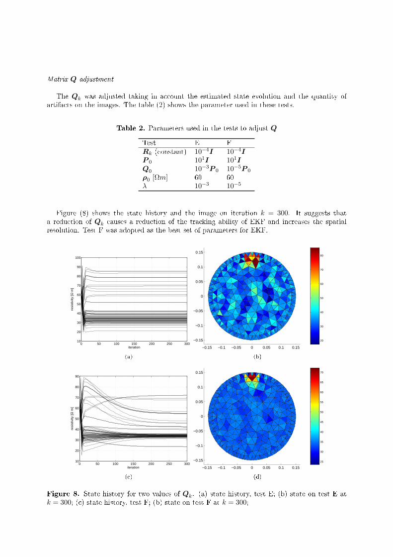
The Qk was adjusted taking in account the estimated state evolution and the quantity ofartifacts on the images. The table (2) shows the parameter used in these tests.

Table 2. Parameters used in the tests to adjust Q

Test E FRk (constant) 10−4I 10−4IP 0 101I 101IQ0 10−3P 0 10−5P 0

ρ0 [Ωm] 60 60λ 10−3 10−5

Figure (8) shows the state history and the image on iteration k = 300. It suggests thata reduction of Qk causes a reduction of the tracking ability of EKF and increases the spatialresolution. Test F was adopted as the best set of parameters for EKF.

0 50 100 150 200 250 30010

20

30

40

50

60

70

80

90

100

resi

stiv

ity [Ω

m]

iteration

(a)−0.15 −0.1 −0.05 0 0.05 0.1 0.15

−0.15

−0.1

−0.05

0

0.05

0.1

0.15

20

30

40

50

60

70

80

(b)

0 50 100 150 200 250 30010

20

30

40

50

60

70

80

90

resi

stiv

ity [Ω

m]

iteration

(c)−0.15 −0.1 −0.05 0 0.05 0.1 0.15

−0.15

−0.1

−0.05

0

0.05

0.1

0.15

25

30

35

40

45

50

55

60

65

70

(d)

Figure 8. State history for two values of Qk. (a) state history, test E; (b) state on test E atk = 300; (c) state history, test F; (b) state on test F at k = 300;

5.3.2. When the object is at the center of the domain The set of parameters from test F wereused in test G. Figure (9) shows the state history, the image at iteration k = 300, and theobservation residue. Table (3) shows the parameters used.

0 50 100 150 200 250 30010

20

30

40

50

60

70

80

90

100

110

resi

stiv

ity [Ω

m]

iteration

(a)

0 50 100 150 200 250 30010

−3

10−2

10−1

100

obse

rvat

ion

resi

due

(V)

iteration

residuesuperior limit

(b)

−0.15 −0.1 −0.05 0 0.05 0.1 0.15

−0.15

−0.1

−0.05

0

0.05

0.1

0.15

30

40

50

60

70

80

(c)

Figure 9. Test G. (a) State history; (b) Observation residue; (c) State at k = 300.

It can be observed that the observation residue is lower in test G than in test F. Whenthe object is in the center, errors in the state estimation have low inuence in the predictedmeasurements. Therefore, a direct comparison between observation residues is not fair. Sincethe tracking ability can be improved, another set of parameters was proposed, based on theparameters of test G. A smaller value of matrix Rk was attempted. Table (3) shows theparameters used.

Table 3. Parameters used in the tests to adjust R

Test G HRk (constant) 10−4I 10−6IP 0 101I 101IQ0 10−5P 0 10−5P 0

ρ0 [Ωm] 60 60λ 10−5 10−5

Figure (10) shows the state history, the image at iteration k = 300 and the observationresidue.

0 50 100 150 200 250 300−20

0

20

40

60

80

100

120

resi

stiv

ity [Ω

m]

iteration

(a)

0 50 100 150 200 250 30010

−3

10−2

10−1

100

obse

rvat

ion

resi

due

(V)

iteration

residuesuperior limit

(b)

−0.15 −0.1 −0.05 0 0.05 0.1 0.15

−0.15

−0.1

−0.05

0

0.05

0.1

0.15

30

40

50

60

70

80

(c)

Figure 10. Test H. (a) State history; (b) Observation residue; (c) State at k = 300.

In about 25 iterations test H converged. Comparing test G and test H, clearly the trackingability improved by reducing Rk.

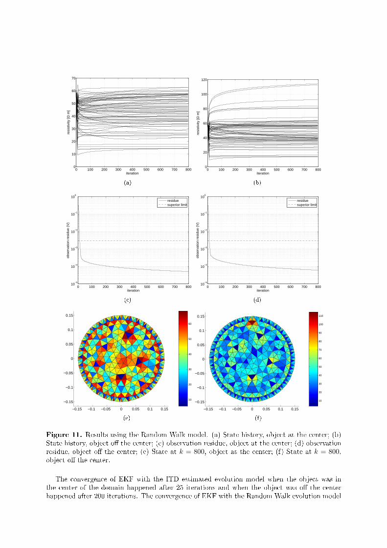
6. Performance of EKF with the Random Walk Evolution ModelIn this subsection the performance of EKF using the Random Walk Model is presented. Figure(11) shows the state history, the observation residue and the state at iteration k = 800 for thetwo dierent object positions with the Random Walk model. The object was not visible in thecenter although the observation residue lies within three standard deviation range. It can beobserved that there are many artifacts in both images.

0 100 200 300 400 500 600 700 8000

10

20

30

40

50

60

70

resi

stiv

ity [Ω

m]

iteration

(a)

0 100 200 300 400 500 600 700 8000

20

40

60

80

100

120

resi

stiv

ity [Ω

m]

iteration

(b)

0 100 200 300 400 500 600 700 80010

−5

10−4

10−3

10−2

10−1

100

obse

rvat

ion

resi

due

(V)

iteration

residuesuperior limit

(c)

0 100 200 300 400 500 600 700 80010

−5

10−4

10−3

10−2

10−1

100

obse

rvat

ion

resi

due

(V)

iteration

residuesuperior limit

(d)

−0.15 −0.1 −0.05 0 0.05 0.1 0.15

−0.15

−0.1

−0.05

0

0.05

0.1

0.15

10

20

30

40

50

60

(e)−0.15 −0.1 −0.05 0 0.05 0.1 0.15

−0.15

−0.1

−0.05

0

0.05

0.1

0.15

10

20

30

40

50

60

70

80

90

100

110

(f)

Figure 11. Results using the Random Walk model. (a) State history, object at the center; (b)State history, object o the center; (c) observation residue, object at the center; (d) observationresidue, object o the center; (e) State at k = 800, object at the center; (f) State at k = 800,object o the center.

The convergence of EKF with the ITD estimated evolution model when the object was inthe center of the domain happened after 25 iterations and when the object was o the centerhappened after 200 iterations. The convergence of EKF with the Random Walk evolution model

when the object was in the center of the domain ocurred after 800 iterations and when the objectwas o the center did not happened within 800 iterations. The tracking ability was accelerated32 times by the use of the ITD estimated evolution model when the object was in the center ofthe domain and mores than 4 times when the object was o the center of the domain.

7. Final CommentsThe results show that the Ibrahim Time Domain method can be used to estimate the evolutionmodel based on a sequence of images obtained by a sensitivity matrix algorithm. Althoughthe resistivity distribution obtained by the sensitivity matrix algorithm is underestimated, thetracking ability of the EKF was improved when compared to the use of the Random Walk modelfor the evolution model.

The computational eort to implement the direct identication of the transition matrix seemsto be justied since the tracking ability improved approximately thirty two times when the objectwas in the center and more than four times when the object was near the boundary.

The use of observation vector of dimension 1024 instead of 32 caused each iteration to belonger but, on the other hand, the P update can be performed according to the equation (5)and an oscillation with periodicity 32 was avoided.

AcknowledgmentsThe authors want to express their gratitude to Marko Vauhkonen, for suggesting the use of anevolution model other than random walk model. The authors are also grateful for the nancialaid from The State of São Paulo Research Foundation, processes 01/05303-4, 05/01088-2 and07/04069-4.

8. References[1] Cheney M, Isaacson D and Newell J C 1999 Society for Industrial and Applied Mathematics 41 85101[2] Trigo F C, Lima R G and Amato M B P 2004 IEEE Transactions on Biomedical Engineering 51 7281[3] Maybeck P S 1979 Stochastic models, estimation and control 1st ed vol 1 (New York: Academic Press Inc.)[4] Jazwinski A H 1970 Stochastic Processes and Filtering Theory (New York: Academic Press Inc.)[5] Vauhkonen M, Karjalainen P A and Kaipio J P 1998 IEEE Transactions on Biomedical Engineering 45

486493[6] Kaipio J P, Karjalainen P A and Somersalo E 1999 Annals-New York Academy Of Sciences 430439[7] Kim K Y, Kim B S, Kim M C, Lee Y and Vauhkonen M 2001 Measurement Science and Technology 10321039[8] Kim K Y, Kang S I, Kim M C, Kim S, Lee Y and Vauhkonen M 2002 IEEE Transactions on Magnetics 38

13011304[9] Trigo F C 2005 Estimação não linear de parâmetros através dos ltros de Kalman na tomograa por

impedância elétrica Ph.D. thesis Escola Politécnica da Universidade de São Paulo São Paulo[10] Kim B S, Kim M C, Kim S and Kim K Y 2004 Measurement Science and Technology 15 21132123[11] Ibrahim S R and Mikulcik E C 1973 Shock and vibration 43 2137[12] Ibrahim S R and Mikulcik E C 1977 Shock and vibration 47 183198[13] Trigo F C 2001 Filtro Estendido de Kalman Aplicado à Tomograa por Impedância Elétrica Master's thesis

Escola Politécnica da Universidade de São Paulo São Paulo[14] Moura F S 2006 Identicação da Matriz de Transição do Modelo de Evolução do Filtro Estendido de Kalman

na Tomograa por Impedância Elétrica (São Paulo)[15] Ewins D J 1984 Modal Testing: Theory and Pratice 1st ed (New York: Research Studies Press LTD.)[16] Neto L S F 2004 Um método para análise modal de estruturas submetidas a excitações ambientes Master's

thesis Escola Politécnica da Universidade de São Paulo São Paulo[17] Moura F S, Aya J C C, Mirandola L A S, Nan P C, Schweder R K and Lima R G 2005 International Congress

of Mechanical Engineering[18] Hua P, Woo E J, Webster J G and Tompkins W J 1993 IEEE Transactions on Biomedical Engineering 40

335343[19] Brogan W L 1991 Modern Control Theory 3rd ed (New Jersey: Prentice Hall)