Multiple Adaptive Fading Schmidt-Kalman Filter for Unknown Bias

Research ArticleMultiple Adaptive Fading Schmidt-Kalman Filterfor Unknown Bias

Tai-Shan Lou, Zhi-Hua Wang, Meng-Li Xiao, and Hui-Min Fu

School of Aeronautical Science and Engineering, BeiHang University, Beijing 100191, China

Correspondence should be addressed to Zhi-Hua Wang; [email protected]

Received 24 September 2014; Accepted 12 November 2014; Published 24 November 2014

Academic Editor: Zheng-Guang Wu

Copyright © 2014 Tai-Shan Lou et al. This is an open access article distributed under the Creative Commons Attribution License,which permits unrestricted use, distribution, and reproduction in any medium, provided the original work is properly cited.

Unknown biases in dynamic and measurement models of the dynamic systems can bring greatly negative effects to the stateestimates when using a conventional Kalman filter algorithm. Schmidt introduces the “consider” analysis to account for errorsin both the dynamic and measurement models due to the unknown biases. Although the Schmidt-Kalman filter “considers” thebiases, the uncertain initial values and incorrect covariance matrices of the unknown biases still are not considered. To solve thisproblem, a multiple adaptive fading Schmidt-Kalman filter (MAFSKF) is designed by using the proposed multiple adaptive fadingKalman filter to mitigate the negative effects of the unknown biases in dynamic or measurement model. The performance of theMAFSKF algorithm is verified by simulation.

1. Introduction

An underlying assumption of the Kalman filter is that thedynamic andmeasurement equations can be accuratelymod-eled without any colored noise or unknown biases. However,in practice, these dynamic and measurement models includesome additional biases, which always bring greatly negativeeffects to the state estimate.

There are many methodologies to deal with theseunknown biases. Ignoring them and augmenting them toestimate are two common approaches. Based on the sen-sitivity to the unknown bias, some techniques have beenproposed, such as Η

∞filtering [1, 2], set-valued estimation

[3], and Schmidt-Kalman filter (SKF) [4]. Schmidt proposeda “consider” analysis, which is the cornerstone of the SKF,to account for errors in both the dynamic and measurementmodels due to the unknown biases when the biases areconsidered as constants and remain unchanged [4]. Based ona minimum variance approach, the key idea of the SKF isthe “consider” analysis that the preestimated bias covarianceis formulated to update the state and covariance estimates,but these biases themselves are not estimated directly. The“consider” approach is especially useful when the unknown

biases are low observable or when the extra computationalpower to estimate them is not worth [5].

After Schmidt, the “consider” approach for parametershas received much attention in recent years. The SKF is alsocalled the consider Kalman filter (CKF) after its developer.Jazwinski provides the detailed derivation of the CKF inhis book [6]. Subsequently, Tapley et al. amply descript theCKF and derivate a different formulation [7]. Zanetti andSouza introduce the UDU formulation into the SKF andprovide a numerically stability, recursive implementation ofthe UDU SKF [8]. Bierman analyzes the effects on filteringaccuracy of the unestimated biases and incorrect a prioricovariance statistics and proposes a sensitivity matrix toevaluate them [9]. Woodbury et al. give novelty insight intoconsidering biases in the measurement model and verifythe negative effect of the errors in the initial parameter andcovariance estimates [5, 10]. Chee and Forbes propose anorm-constrained consider Kalman filtering by taking intoaccount the constraint on the state estimate and apply it to anonlinear attitude estimation problem [11].

However, how to mitigate these negative effects from theinitial state and covariance values of the unknown biasesin the SKF has not attracted much attention. In fact, when

Hindawi Publishing CorporationMathematical Problems in EngineeringVolume 2014, Article ID 623930, 8 pageshttp://dx.doi.org/10.1155/2014/623930

http://dx.doi.org/10.1155/2014/623930

2 Mathematical Problems in Engineering

the inaccurate initial and covariance values, that is to say thebiases are not accurately modeled, are used to update thestate and covariance estimates, the accuracy of the state andcovariance estimates may greatly degrade. Fortunately, theadaptive technique is proposed to improve the convergenceof the filtering. As a member of the adaptive Kalman filteringalgorithms, the adaptive fading Kalman filtering algorithmis proposed to use a single adaptive fading factor (FF) as amultiplier to the dynamic or measurement noise covariancewhen the information about the dynamic or measurementmodel is incomplete [12–15]. Then, to consider the complexsystems with multivariable, a single fading factor is notsufficiently used, and so the multiple fading factor, which isthe footstone of multiple adaptive fading Kalman filtering(MAFKF), is proposed to reflect corrective effects of themultivariable in filtering [16–19]. But in the MAFKF themultiple fading factors are only used as a multiplier for thelast posteriori covariance of the states, and the method for thewhole priori covariance of the states is not considered untilnow.

To consider the incomplete information from both thecovariance of the states and noises, the MAFKF is proposedto use themultiple fading factor as a multiplier on the outsideof the whole priori error covariance equation. The proposedMAFKF not only considers the uncertainty of the models butalso adjusts the covariance of inaccurate modeled noises. Inaddition, the multiple fading factors are derived by one-stepapproximate algorithm to decrease the computational com-plexity in the MAFKF algorithm.Then, the multiple adaptivefading Schmidt-Kalman filter (MAFSKF) is designed byusing the aboveMAFKF tomitigate the negative effects of theuncertain parameters in dynamic or measurement model.

This paper is organized as follows. First, the problemstatement with the unknown biases is given. Second, theMAFKF algorithm is proposed to compensate the effect ofinaccuracy information covariance. Third, the MAFSKF isdesigned to mitigate the negative effects of the unknownbiases. Finally, the performance of the MAFSKF algorithm isverified by simulation and the results are discussed as well.

2. Problem Statement

Consider a linear discrete dynamic systemwith the unknownbiases as follows:

x𝑘+1

= Φ𝑘+1|𝑘

x𝑘+Ψ𝑘+1|𝑘

p𝑘+ G𝑘w𝑘

(1a)

z𝑘= H𝑘x𝑘+ N𝑘b𝑘+ k𝑘, (1b)

where x𝑘is the 𝑛 × 1 state vector and z

𝑘is the 𝑚 × 1

measurement vector. Φ𝑘+1|𝑘

and Ψ𝑘+1|𝑘

are the state andbias transition matrices, G

𝑘is the coefficient matrix of the

process noise, H𝑘is the measurement matrix, and N

𝑘is

the measurement bias transition matrix. p𝑘is referred to

as the 𝑛𝑝× 1 dynamical bias vector and b

𝑘is called the

𝑚𝑏× 1 measurement bias vector. w

𝑘and k𝑘are independent

zero-meanGaussian noise processes and their covariance are,respectively,Q

𝑘and R

𝑘. They satisfy

𝐸 [w𝑖w𝑇𝑗] = Q

𝑘𝛿𝑖𝑗,

𝐸 [k𝑖k𝑇𝑗] = R𝑘𝛿𝑖𝑗,

𝐸 [w𝑖k𝑇𝑗] = 0,

(2)

where 𝛿𝑖𝑗is the Kronecker delta function andQ

𝑘> 0, R

𝑘> 0.

Here, the biases p𝑘and b

𝑘, which are considered as

unknown constants and remain the same in filtering, aremodeled as

p𝑘+1

= p𝑘, p0= p,

b𝑘+1

= b𝑘, b0= b.

(3)

The initial states x0and biases p

0and b

0are assumed to

be independent of the Gaussian noise {w𝑘} and {k

𝑘} and be

Gaussian random variables with

𝐸 [x0] = x0, 𝐸 [(x

0− x0) (x0− x0)𝑇

] = P0> 0,

𝐸 [p0] = p0, 𝐸 [(p

0− p0) (p0− p0)𝑇

] = Q𝑝0> 0,

𝐸 [b0] = b0, 𝐸 [(b

0− b0) (b0− b0)𝑇

] = Q𝑏0> 0,

𝐸 [(x0− x0) (p0− p0)𝑇

] = C𝑥𝑝0,

𝐸 [(x0− x0) (b0− b0)𝑇

] = C𝑥𝑏0.

(4)

Based on the assumption that the stochastic informationof the unknown biases is incomplete, a multiple adaptivefading Schmidt-Kalman filter is designed to overcome theproblem with the unknown biases.

3. MAFKF Algorithm

Consider the linear discrete stochastic system as follows:

x𝑘+1

= Φ𝑘+1|𝑘

x𝑘+ G𝑘w𝑘, (5a)

z𝑘= H𝑘x𝑘+ k𝑘. (5b)

If the system is observable, the optimal estimate is givenby the conventional Kalman filter [7]. Unfortunately, theinformation is always incomplete in practice, and this leadsthe filter to “learn the wrong state too well” [20]. To compen-sate the effects of the incomplete information, the adaptivefading Kalman filter (AFKF) is proposed to overcome theproblem [12, 13]. When the older data from the currentestimate are no longer meaningful due to the erroneousmodel, the negative effects of these data are mitigated by theAFKF. Between theAFKF and the conventional Kalman filter,the big difference is that a constant fading factor is insertedinto the a priori error covariance equation. There are three

Mathematical Problems in Engineering 3

representative types with a single fading factor to be assigned[12, 13, 15, 21],

P𝑘+1|𝑘

= 𝜆𝑘Φ𝑘+1|𝑘

P𝑘Φ𝑇

𝑘+1|𝑘+ G𝑘Q𝑘G𝑇𝑘, (6a)

P𝑘+1|𝑘

= Φ𝑘+1|𝑘

P𝑘Φ𝑇

𝑘+1|𝑘+ 𝜆𝑘G𝑘Q𝑘G𝑇𝑘, (6b)

P𝑘+1|𝑘

= 𝜆𝑘(Φ𝑘+1|𝑘

P𝑘Φ𝑇

𝑘+1|𝑘+ G𝑘Q𝑘G𝑇𝑘) . (6c)

However, only one constant fading factor cannot “weight”the covariance of all states, and the optimal filtering cannotbe guaranteed, especially for the complicated multivariablesystems. To overcome the shortcomings of the single fadingfactor, Zhou et al. [16] proposed a suboptimal multiple fadingextendedKalmanfilter by using the error covariance equationof (6a), in which the single fading factor 𝜆

𝑘is substituted by

a multiple fading factor matrix S𝑘, and the orthogonality of

the residual errors is remained. Zhou et al. also gave one-step approximation algorithm of the multiple fading factorand verified the affectivity of the multiple fading factor infiltering. The equation of (6b) and (6c) was considered fora single fading factor in the literature [13, 16]. But for themultiple fading factor, no researchers consider the last twoequations. To consider the incomplete information fromboththe covariance of the states and noises, the multiple fadingfactor should be inserted on the outside of the a priori errorcovariance equation. Hence, based on (6c) as the comment inthe literature [17], the proposed MAFKF is defined as

P𝑘+1|𝑘

= S𝑘+1(Φ𝑘+1|𝑘

P𝑘Φ𝑇

𝑘+1|𝑘+ G𝑘Q𝑘G𝑇𝑘) , (7)

where S𝑘+1

= diag{𝜆1,𝑘+1

, 𝜆2,𝑘+1

, . . . , 𝜆𝑛,𝑘+1

}; 𝜆𝑖,𝑘+1

≥ 1 (𝑖 =

1, 2, . . . , 𝑛) is the multiple fading factor.In the conventional Kalman filter, the predicted residual

vector can be expressed as𝛾𝑘+1

= z𝑘+1−H𝑘+1

x𝑘+1|𝑘

(8)

and the corresponding innovation covariance matrix can becalculated as

Ω𝑘+1

= 𝐸 [𝛾𝑘+1𝛾𝑇

𝑘+1] = H

𝑘+1P𝑘+1|𝑘

H𝑇𝑘+1+ R𝑘+1, (9)

where P𝑘+1|𝑘

is a priori error covariance of the linear Kalmanfilter.

In the optimal linear Kalman filter, there is an orthogonalprinciple that the predicted residual sequence {𝛾

𝑘} ismutually

orthogonal when the optimal gain matrix is calculated online[16].The optimal gainmatrix is obtained in the linear Kalmanfilter by minimizing the following equation:

𝐸 [(x𝑘+1− x𝑘+1) (x𝑘+1− x𝑘+1)𝑇

] , 𝑘 = 0, 1, 2, . . . , (10)

and then the following equation is satisfied:

𝐸 [𝛾𝑘+𝑗+1𝛾𝑇

𝑘+1] = 0, 𝑘 = 0, 1, 2, . . . , 𝑗 = 1, 2, 3, . . . . (11)

Substituting (8) into the left formula of (11), the result can beobtained as follows:𝐸 [𝛾𝑘+𝑗+1𝛾𝑇

𝑘+1]

= H𝑘+𝑗+1Φ𝑘+𝑗+1|𝑘+𝑗

[I − K𝑘+𝑗

H𝑘+𝑗] ⋅ ⋅ ⋅Φ

𝑘+3|𝑘+2

× [I − K𝑘+2

H𝑘+2]Φ𝑘+2|𝑘+1

Λ𝑘+1, 𝑗 = 1, 2, 3, . . . ,

(12)

where Λ𝑘+1

is defined as (for all 𝑘 = 0, 1, 2, 3, . . .)

Λ𝑘+1

= P𝑘+1|𝑘

H𝑇𝑘+1− K𝑘+1Ω𝑘+1. (13)

Substituting the optimal gain matrix K𝑘+1

=

P𝑘+1|𝑘

H𝑇𝑘+1[H𝑘+1

P𝑘+1|𝑘

H𝑇𝑘+1

+ R𝑘+1]−1 of the linear Kalman

filter into (13), Λ𝑘+1

is identically zero, and this means that(12) is identical to zero, too. The orthogonal principle is rightwhen the optimal gain matrix is inserted.

In practice, the dynamic model of the stochastic systemalways is partially known, and so the real covariance matrixmay be increased by the unknown information, and it isdifferent from the theoretical covariance Ω

𝑘+1in (9). Thus,

the real autocovariance matrix 𝐸[𝛾𝑘+𝑗+1𝛾𝑇

𝑘+1] may not be

identically zero. For (12), if the multiple fading factor in (7)is chosen so that Λ

𝑘+1= 0, then the gain matrix K

𝑘+1is

optimal. From the above, it can be seen that ifK𝑘+1

is optimal,Λ𝑘+1

= 0 in (12), and if Λ𝑘+1

= 0, K𝑘+1

is optimal. The basicidea to design the adaptive fading filtering is obtained fromaforementioned analysis.

Hence, the optimality of the Kalman filter can be evalu-ated by the following function constructed:

𝑔 (𝜆𝑘+1) =

𝑛

∑

𝑖=1

𝑚

∑

𝑗=1

Λ2

𝑖𝑗,𝑘+1, (14)

where Λ𝑘+1

= (Λ𝑖𝑗,𝑘+1

)𝑛𝑚

and 𝜆𝑘+1

= [𝜆1,𝑘+1

, 𝜆2,𝑘+1

, . . . ,

𝜆𝑛,𝑘+1

]𝑇. 𝑔(𝜆

𝑘+1) describes the distance to the optimal esti-

mate in linear Kalman filter. When 𝑔(𝜆𝑘+1) is minimum, a

suboptimal estimate, which is the most close to the optimalestimate, will be obtained. Hence, we can obtain the multiplefading factor S

𝑘by minimizing (14) as follows:

min𝜆𝑘

𝑔 (𝜆𝑘) . (15)

Obviously, (15) can be solved by using any unconstrainedmultivariate nonlinear programming methods. However,finding the optimal solution is not suitable for the onlinestate estimate [16]. Hence, a one-step approximate algorithmis proposed to obtain the multiple fading factors S

𝑘for the

online calculating.Here, when the a priori characters of the system are

roughly known, we can assume that

𝜆1,𝑘+1

: 𝜆2,𝑘+1

: ⋅ ⋅ ⋅ : 𝜆𝑛,𝑘+1

= 𝛽1: 𝛽2: ⋅ ⋅ ⋅ : 𝛽

𝑛(16)

and then set

𝜆𝑖,𝑘+1

= 𝛽𝑖𝜏𝑘+1, 𝑖 = 1, 2, . . . , 𝑛, (17)

where 𝛽𝑖≥ 1 is the constant from the prognosis to the state

and 𝜏𝑘+1

is the undetermined factor.Substituting the Kalman gain matrix K

𝑘+1=

P𝑘+1|𝑘

H𝑇𝑘+1[H𝑘+1

P𝑘+1|𝑘

H𝑇𝑘+1

+ R𝑘+1]−1 into the Λ

𝑘+1= 0

generates

P𝑘+1|𝑘

H𝑇𝑘+1{I − [H

𝑘+1P𝑘+1|𝑘

H𝑇𝑘+1+ R𝑘+1]−1

Ω𝑘+1} = 0.

(18)

It is obvious that one sufficient condition to establish (18) is

[H𝑘+1

P𝑘+1|𝑘

H𝑇𝑘+1+ R𝑘+1]−1

Ω𝑘+1

= I (19)


or

H𝑘+1

P𝑘+1|𝑘

H𝑇𝑘+1

= Ω𝑘+1− R𝑘+1. (20)

Substituting (7) into (20) and reorganizing it gives

H𝑘+1

S𝑘+1(Φ𝑘+1|𝑘

P𝑘Φ𝑇

𝑘+1|𝑘+ G𝑘Q𝑘G𝑇𝑘)H𝑇𝑘+1

= Ω𝑘+1− R𝑘+1.

(21)

From the right part of (21), it is seen that the multiple fadingfactor S

𝑘+1is valid when Ω

𝑘+1− R𝑘+1

> 0 is satisfied[16]. For the measurement covariance matrix R

𝑘+1> 0, a

softening factor 𝜀 ≥ 1, which is usually given by experience,is introduced to weaken the excessive adjust of the multiplefading factor and smooth the state estimates. Hence, (21) isrestructured as

H𝑘+1

S𝑘+1(Φ𝑘+1|𝑘

P𝑘Φ𝑇


= Ω𝑘+1− 𝜀R𝑘+1.

(22)

Based on the property of commutative matrices in traceoperator tr[𝐴𝐵] = tr[𝐵𝐴], the trace of both sides in (22) iscalculated as

tr [S𝑘+1(Φ𝑘+1|𝑘

P𝑘Φ𝑇


H𝑘+1] = tr [Ω

𝑘+1− 𝜀R𝑘+1] .

(23)

Simplify (23) as

tr [S𝑘+1

M𝑘+1] = tr [O

𝑘+1] , (24)

where

M𝑘+1

= (Φ𝑘+1|𝑘

P𝑘Φ𝑇


H𝑘+1, (25)

O𝑘+1

= Ω𝑘+1− 𝜀R𝑘+1. (26)

In fact, the real residual covariance matrixΩ𝑘+1

in (26) isunknown but can be evaluated by the following equation [16]:

Ω𝑘+1

=

{{

{{

{

𝛾1𝛾𝑇

1, 𝑘 = 1

𝜌Ω𝑘+ 𝛾𝑘+1𝛾𝑇

𝑘+1

1 + 𝜌, 𝑘 > 1,

(27)

where 𝜌 is a forgetting factor, which is 0 < 𝜌 ≤ 1.Substituting (17) into (24) gives

tr{{{

{{{

{

[[[

[

𝛽1𝜏𝑘+1

𝛽2𝜏𝑘+1

d𝛽𝑛𝜏𝑘+1

]]]

]

M𝑘+1

}}}

}}}

}

= tr [O𝑘+1]

(28)

and then 𝜏𝑘+1

is calculated as

𝜏𝑘+1

=tr [O𝑘+1]

∑𝑛

𝑖=1𝛽𝑖M𝑖𝑖,𝑘+1

. (29)

Synthesizing condition 𝜆𝑖,𝑘+1

≥ 1 and (17), (29) gives

𝜆𝑖,𝑘+1

= max {1, 𝛽𝑖𝜏𝑘+1} , 𝑖 = 1, 2, . . . , 𝑛. (30)

Algorithm 1 (one-step approximate MAFKF). A discrete-timemultiple adaptive fadingKalmanfilter is proposed by thefollowing equations when the information about the linearstochastic system is incomplete:

x𝑘+1|𝑘

= Φ𝑘+1|𝑘

x𝑘, (31a)

P𝑘+1|𝑘

= S𝑘+1(Φ𝑘+1|𝑘

P𝑘Φ𝑇

𝑘+1|𝑘+ G𝑘Q𝑘G𝑇𝑘) , (31b)

K𝑘+1

= P𝑘+1|𝑘

H𝑇𝑘+1[H𝑘+1

P𝑘+1|𝑘

H𝑇𝑘+1+ R𝑘+1]−1

, (31c)

x𝑘|𝑘= x𝑘|𝑘−1

+ K𝑘𝛾𝑘+1, (31d)

P𝑘= (I − K

𝑘H𝑘)P𝑘|𝑘−1

, (31e)

where

𝛾𝑘+1

= z𝑘+1−H𝑘+1

x𝑘+1|𝑘

,

S𝑘+1

= diag {𝜆1,𝑘+1

, 𝜆2,𝑘+1

, . . . , 𝜆𝑛,𝑘+1

} ,

𝜆𝑖,𝑘+1

= max {1, 𝛽𝑖𝜏𝑘+1} , 𝑖 = 1, 2, . . . , 𝑛,

𝜏𝑘+1

=tr [O𝑘+1]

∑𝑛


,

M𝑘+1

= (Φ𝑘+1|𝑘

P𝑘Φ𝑇


H𝑘+1,

O𝑘+1

= Ω𝑘+1− 𝜀R𝑘+1,

Ω𝑘+1

=

{{

{{

{

𝛾1𝛾𝑇

1, 𝑘 = 1


𝑘+1

1 + 𝜌, 𝑘 > 1.

(32)

To consider the difference between the states and themultisource incomplete information, the MAFKF algorithmis proposed to use the multiple fading factor as a multiplierfor the whole a priori covariance P

𝑘+1|𝑘of the states and

mitigate the negative effects of the uncertainties. Comparedto the single adaptive fading Kalman filter, the MAFKF isintroduced into the multiple fading factor and adjusts eachcomponent of the state vector by different fading factor toperform better. In addition, the multiple fading factor isderived by one-step approximate algorithm to decrease thecomputational complexity.

The asymptotical stability of the proposed MAFKF iseasily proved in the literature [15], by using the results in theliterature [22–24].

Remarks. The proportionality factor 𝛽𝑖of the multiple fading

factor S𝑘can be designed with the a priori knowledge of the

states before the filtering [16].

4. MAFSKF for the Unknown Biases

The unknown biases in the problem statement (1a) and (1b)have a greatly negative impact on the filter accuracy andeven result in filter divergence [6]. In the SKF algorithm, thecovariance of unknown biases is used to update the state andcovariance estimates but is not estimated directly.However, as


the most important part in the SKF, the unknown covariancematrices Q𝑝

0and Q𝑏

0and the uncertain initial values of the

unknown biases are still not considered. To consider thenegative effects in the SKF filtering from this incompleteinformation, the MAFKF is proposed to solve this problem.Based on the two aforementioned aspects, the MAFSKF isdesigned by using the MAFKF and the conventional SKF.

Similarly to (8) and (9) in the conventional Kalmanfilter, the predicted residual vector and the correspondinginnovation covariance matrix in SKF can be expressed as

𝛾𝑘+1

= z𝑘+1−H𝑘+1

x𝑘+1|𝑘

− N𝑘+1

b, (33)

Ω𝑘+1

= 𝐸 [𝛾𝑘+1𝛾𝑇

𝑘+1] = H

𝑘+1P𝑘+1|𝑘

H𝑇𝑘+1+ N𝑘+1

C𝑏𝑇𝑘+1|𝑘

H𝑇𝑘+1+H𝑘+1

C𝑏𝑘+1|𝑘

N𝑇𝑘+1

+ N𝑘+1

Q𝑏0N𝑇𝑘+1+ R𝑘+1,

(34)

where the unknown real residual covariance matrix Ω𝑘+1

iscalculated by (27).

The incomplete information, coming from the unknownbiases in models, can be obtained from (27), (33), and (34).So the multiple fading factor can be calculated from (27) and(34) and used to compensate the corresponding covariancematrix and autocovariance matrix.

The SKF algorithm is derived as follows [4, 25]. First, theunknown biases are augmented into the states and the newaugmented system is produced. Second, the standard linearKalman filter is derived from the augmented system. Third,the estimation equations for the biases are thrown away, butthe covariance between the states and biases is retrained.From the recursions in SKF [25], the a priori error covarianceincludesP𝑘+1|𝑘

= Φ𝑘+1|𝑘

P𝑘Φ𝑇

𝑘+1|𝑘+Φ𝑘+1|𝑘

C𝑝𝑘Ψ𝑇

𝑘+1|𝑘+Ψ𝑘+1|𝑘

C𝑝𝑇𝑘Φ𝑇

𝑘+1|𝑘

+Ψ𝑘+1|𝑘

Q𝑝0Ψ𝑇

𝑘+1|𝑘+ G𝑘Q𝑘G𝑇𝑘,

C𝑝𝑘+1|𝑘

= Φ𝑘+1|𝑘

C𝑝𝑘+Ψ𝑘+1|𝑘

Q𝑝0,

C𝑏𝑘+1|𝑘

= Φ𝑘+1|𝑘

C𝑏𝑘.

(35)

From the recursive process, the three above covari-ance matrices should be adjusted by the multiple fad-ing factor S

𝑘+1, for the incomplete information of the

unknown biases. The multiple fading factor S𝑘+1

=

diag{𝜆1,𝑘+1

, 𝜆2,𝑘+1

, . . . , 𝜆𝑛,𝑘+1

} is calculated for the augmentedsystem like the proposed MAFKF. Under assumption that𝜆𝑖,𝑘+1

= max{1, 𝛽𝑖𝜏𝑘+1}, 𝑖 = 1, 2, . . . , 𝑛, 𝜏

𝑘+1is calculated as

in (29), and O𝑘+1

still remains the same, but M𝑘+1

in (29) ischanged into

M𝑘+1

= (Φ𝑘+1|𝑘

P𝑘Φ𝑇


C𝑝𝑘Ψ𝑇

𝑘+1|𝑘

+Ψ𝑘+1|𝑘

C𝑝𝑇𝑘Φ𝑇

𝑘+1|𝑘

+ Ψ𝑘+1|𝑘

Q𝑝0Ψ𝑇


H𝑘+1

+Φ𝑘+1|𝑘

C𝑏𝑘N𝑇𝑘+1

H𝑘+1.

(36)

From the analysis above, a multiple adaptive fadingSchmidt-Kalman filter is proposed to mitigate the negativeeffects of the unknown biases.

Algorithm 2 (one-step approximate MAFSKF). Based on theone-step approximateMAFKF algorithm, amultiple adaptivefading Schmidt-Kalman filter is proposed by the followingequations when the information about the linear stochasticsystem is incomplete:

x𝑘+1|𝑘

= Φ𝑘+1|𝑘

x𝑘+Ψ𝑘+1|𝑘

p, (37a)

P𝑘+1|𝑘

= S𝑘+1(Φ𝑘+1|𝑘

P𝑘Φ𝑇


C𝑝𝑘Ψ𝑇

𝑘+1|𝑘

+Ψ𝑘+1|𝑘

C𝑝𝑇𝑘Φ𝑇

𝑘+1|𝑘

+ Ψ𝑘+1|𝑘

Q𝑝0Ψ𝑇

𝑘+1|𝑘+ G𝑘Q𝑘G𝑇𝑘) ,

C𝑝𝑘+1|𝑘

= S𝑘+1(Φ𝑘+1|𝑘

C𝑝𝑘+Ψ𝑘+1|𝑘

Q𝑝0) ,

C𝑏𝑘+1|𝑘

= S𝑘+1(Φ𝑘+1|𝑘

C𝑏𝑘) ,

(37b)

K𝑘+1

= [P𝑘+1|𝑘

H𝑇𝑘+1+ C𝑏𝑘+1|𝑘

N𝑇𝑘+1]Ξ−1

𝑘+1, (37c)

Ξ𝑘+1

= H𝑘+1

P𝑘+1|𝑘

H𝑇𝑘+1+ N𝑘+1


H𝑇𝑘+1

+H𝑘+1

C𝑏𝑘+1|𝑘

N𝑇𝑘+1

+ N𝑘+1

Q𝑏0N𝑇𝑘+1+ R𝑘+1,

(37d)

x𝑘+1

= x𝑘+1|𝑘

+ K𝑘+1𝛾𝑘+1, (37e)

P𝑘+1

= (I − K𝑘+1

H𝑘+1)P𝑘+1|𝑘

− K𝑘+1

N𝑘+1


,

C𝑝𝑘+1

= (I − K𝑘+1

H𝑘+1)C𝑝𝑘+1|𝑘

,

C𝑏𝑘+1

= (I − K𝑘+1

H𝑘+1)C𝑏𝑘+1|𝑘

− K𝑘+1

N𝑘+1

Q𝑏0,

(37f)

where𝛾𝑘+1

= z𝑘+1−H𝑘+1

x𝑘+1|𝑘

− N𝑘+1

b,

S𝑘+1

= diag {𝜆1,𝑘+1

, 𝜆2,𝑘+1

, . . . , 𝜆𝑛,𝑘+1

} ,

𝜆𝑖,𝑘+1

= max {1, 𝛽𝑖𝜏𝑘+1} , 𝑖 = 1, 2, . . . , 𝑛,

𝜏𝑘+1

=tr [O𝑘+1]

∑𝑛


,

O𝑘+1

= Ω𝑘+1− 𝜀R𝑘+1,

Ω𝑘+1

=

{{

{{

{

𝛾1𝛾𝑇

1, 𝑘 = 1


𝑘+1

1 + 𝜌, 𝑘 > 1.

(38)

5. Simulation Results and Analysis

To evaluate the performance of the proposed MAFSKFalgorithm, the spacecraft attitude tracing system with


0 20 40 60 80 100 120 140 160 180 2000

0.1

0.2

0.3

0.4

0.6

0.5

Step

p

Unk

now

n bi

asp

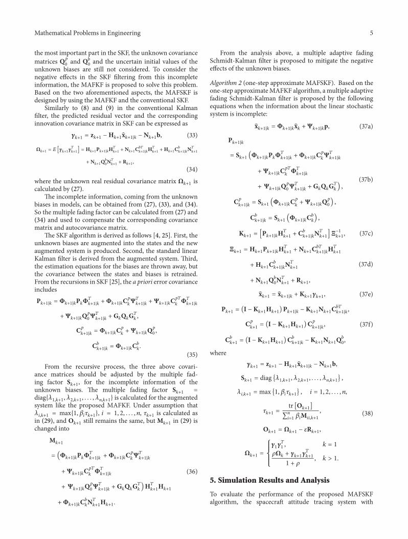
Figure 1: Values of the unknown bias.

the gyroscope as a measurement sensor is considered [26].The spacecraft attitude tracking system, which is mainlyused to enhance and track the spacecraft drift signal, iscorrupted by the unknown bias. The corresponding discrete-time dynamic stochastic system is expressed as

x𝑘+1

= [0 1

−0.85 1.70] x𝑘+ [

0.0129

−1.2504] p𝑘+ [0

1]w𝑘, (39)

z𝑘= [0 1] x

𝑘+ k𝑘. (40)

As in the literature [21], we assumed that x = [𝑥1, 𝑥2]𝑇,w𝑘∼ 𝑁(0, 0.01

2

), and k𝑘∼ 𝑁(0, 0.01

2

). The true state x0=

[2, 1]𝑇 and the unknown bias p

0∼ 𝑁(0, 0.5

2

) were added tothe dynamic equation (39). The initial estimates of the statex0= [1.8, 0.9]

𝑇, and bias p0= 0. In simulation, the dynamic

system is disturbed by some external disturbances, and thevalues of the unknown biases p

𝑘are plotted in Figure 1. The

MAFSKF and SKF use Q𝑝 = 0.001 × 0.52 as the covarianceof the bias p, which is one thousandth of the real covarianceQ𝑝 = 0.5

2. The constant 𝛽 in MAFSKF algorithm is set as𝛽1= 1 and 𝛽

2= 100, the softening factor 𝜀 is set as 𝜀 = 1, and

the forgetting factor is 𝜌 = 0.95.Each single run lasts for 200 samples and 100Monte Carlo

runs are performed.The rootmean squared errors (RMSE) ofthe state estimate are calculated to compare the performanceof the MAFSKF algorithm and the SKF algorithm at eachepoch. The simulation results are shown in Figures 2–5.

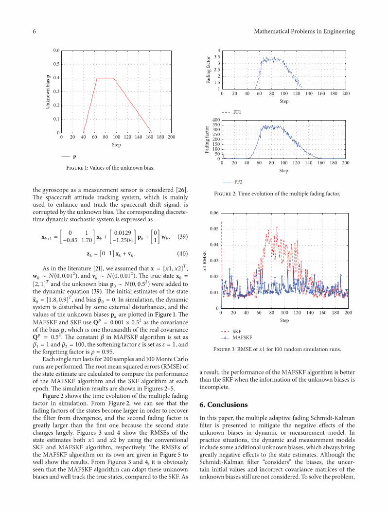
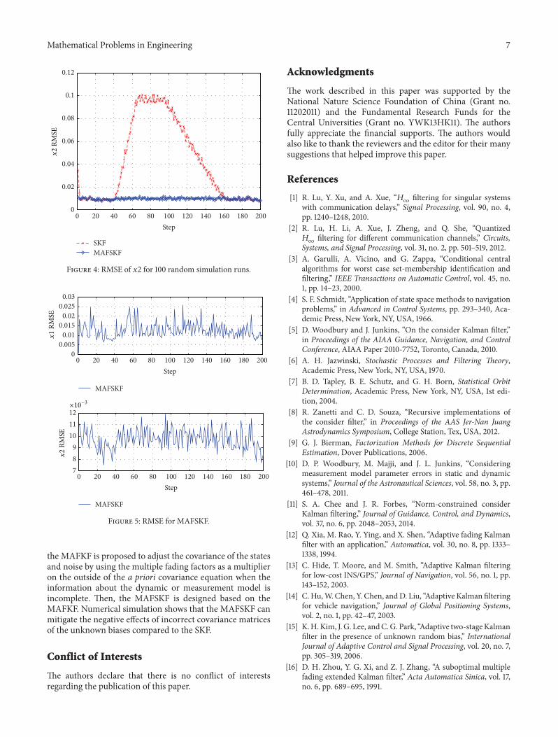
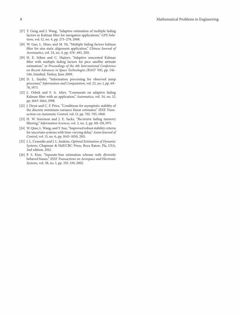
Figure 2 shows the time evolution of the multiple fadingfactor in simulation. From Figure 2, we can see that thefading factors of the states become larger in order to recoverthe filter from divergence, and the second fading factor isgreatly larger than the first one because the second statechanges largely. Figures 3 and 4 show the RMSEs of thestate estimates both 𝑥1 and 𝑥2 by using the conventionalSKF and MAFSKF algorithm, respectively. The RMSEs ofthe MAFSKF algorithm on its own are given in Figure 5 towell show the results. From Figures 3 and 4, it is obviouslyseen that the MAFSKF algorithm can adapt these unknownbiases and well track the true states, compared to the SKF. As

0 20 40 60 80 100 120 140 160 180 2001

1.52

2.53

3.54

Fadi

ng fa

ctor

FF1

0 20 40 60 80 100 120 140 160 180 2000

50100150200250300350400

Step

Step

Fadi

ng fa

ctor

FF2

Figure 2: Time evolution of the multiple fading factor.

0 20 40 60 80 100 120 140 160 180 2000

0.01

0.02

0.03

0.04

0.05

0.06

Step

SKFMAFSKF

x1

RMSE

Figure 3: RMSE of 𝑥1 for 100 random simulation runs.

a result, the performance of the MAFSKF algorithm is betterthan the SKF when the information of the unknown biases isincomplete.

6. Conclusions

In this paper, the multiple adaptive fading Schmidt-Kalmanfilter is presented to mitigate the negative effects of theunknown biases in dynamic or measurement model. Inpractice situations, the dynamic and measurement modelsinclude some additional unknown biases, which always bringgreatly negative effects to the state estimates. Although theSchmidt-Kalman filter “considers” the biases, the uncer-tain initial values and incorrect covariance matrices of theunknownbiases still are not considered. To solve the problem,


0 20 40 60 80 100 120 140 160 180 2000

0.02

0.04

0.06

0.08

0.1

0.12

Step

SKFMAFSKF

x2

RMSE

Figure 4: RMSE of 𝑥2 for 100 random simulation runs.

0 20 40 60 80 100 120 140 160 180 2000

0.0050.01

0.0150.02

0.0250.03

MAFSKF

MAFSKF

0 20 40 60 80 100 120 140 160 180 200789

101112

Step

Step

x1

RMSE

x2

RMSE

×10−3

Figure 5: RMSE for MAFSKF.

the MAFKF is proposed to adjust the covariance of the statesand noise by using the multiple fading factors as a multiplieron the outside of the a priori covariance equation when theinformation about the dynamic or measurement model isincomplete. Then, the MAFSKF is designed based on theMAFKF. Numerical simulation shows that the MAFSKF canmitigate the negative effects of incorrect covariance matricesof the unknown biases compared to the SKF.

Conflict of Interests

The authors declare that there is no conflict of interestsregarding the publication of this paper.

Acknowledgments

The work described in this paper was supported by theNational Nature Science Foundation of China (Grant no.11202011) and the Fundamental Research Funds for theCentral Universities (Grant no. YWK13HK11). The authorsfully appreciate the financial supports. The authors wouldalso like to thank the reviewers and the editor for their manysuggestions that helped improve this paper.

References

[1] R. Lu, Y. Xu, and A. Xue, “𝐻∞

filtering for singular systemswith communication delays,” Signal Processing, vol. 90, no. 4,pp. 1240–1248, 2010.

[2] R. Lu, H. Li, A. Xue, J. Zheng, and Q. She, “Quantized𝐻∞

filtering for different communication channels,” Circuits,Systems, and Signal Processing, vol. 31, no. 2, pp. 501–519, 2012.

[3] A. Garulli, A. Vicino, and G. Zappa, “Conditional centralalgorithms for worst case set-membership identification andfiltering,” IEEE Transactions on Automatic Control, vol. 45, no.1, pp. 14–23, 2000.

[4] S. F. Schmidt, “Application of state space methods to navigationproblems,” in Advanced in Control Systems, pp. 293–340, Aca-demic Press, New York, NY, USA, 1966.

[5] D. Woodbury and J. Junkins, “On the consider Kalman filter,”in Proceedings of the AIAA Guidance, Navigation, and ControlConference, AIAA Paper 2010-7752, Toronto, Canada, 2010.

[6] A. H. Jazwinski, Stochastic Processes and Filtering Theory,Academic Press, New York, NY, USA, 1970.

[7] B. D. Tapley, B. E. Schutz, and G. H. Born, Statistical OrbitDetermination, Academic Press, New York, NY, USA, 1st edi-tion, 2004.

[8] R. Zanetti and C. D. Souza, “Recursive implementations ofthe consider filter,” in Proceedings of the AAS Jer-Nan JuangAstrodynamics Symposium, College Station, Tex, USA, 2012.

[9] G. J. Bierman, Factorization Methods for Discrete SequentialEstimation, Dover Publications, 2006.

[10] D. P. Woodbury, M. Majji, and J. L. Junkins, “Consideringmeasurement model parameter errors in static and dynamicsystems,” Journal of the Astronautical Sciences, vol. 58, no. 3, pp.461–478, 2011.

[11] S. A. Chee and J. R. Forbes, “Norm-constrained considerKalman filtering,” Journal of Guidance, Control, and Dynamics,vol. 37, no. 6, pp. 2048–2053, 2014.

[12] Q. Xia, M. Rao, Y. Ying, and X. Shen, “Adaptive fading Kalmanfilter with an application,” Automatica, vol. 30, no. 8, pp. 1333–1338, 1994.

[13] C. Hide, T. Moore, and M. Smith, “Adaptive Kalman filteringfor low-cost INS/GPS,” Journal of Navigation, vol. 56, no. 1, pp.143–152, 2003.

[14] C. Hu,W. Chen, Y. Chen, andD. Liu, “Adaptive Kalman filteringfor vehicle navigation,” Journal of Global Positioning Systems,vol. 2, no. 1, pp. 42–47, 2003.

[15] K.H.Kim, J.G. Lee, andC.G. Park, “Adaptive two-stageKalmanfilter in the presence of unknown random bias,” InternationalJournal of Adaptive Control and Signal Processing, vol. 20, no. 7,pp. 305–319, 2006.

[16] D. H. Zhou, Y. G. Xi, and Z. J. Zhang, “A suboptimal multiplefading extended Kalman filter,” Acta Automatica Sinica, vol. 17,no. 6, pp. 689–695, 1991.


[17] Y. Geng and J. Wang, “Adaptive estimation of multiple fadingfactors in Kalman filter for navigation applications,” GPS Solu-tions, vol. 12, no. 4, pp. 273–279, 2008.

[18] W. Gao, L. Miao, and M. Ni, “Multiple fading factors kalmanfilter for sins static alignment application,” Chinese Journal ofAeronautics, vol. 24, no. 4, pp. 476–483, 2011.

[19] H. E. Soken and C. Hajiyev, “Adaptive unscented Kalmanfilter with multiple fading factors for pico satellite attitudeestimation,” in Proceedings of the 4th International Conferenceon Recent Advances in Space Technologies (RAST ’09), pp. 541–546, Istanbul, Turkey, June 2009.

[20] D. L. Snyder, “Information processing for observed jumpprocesses,” Information and Computation, vol. 22, no. 1, pp. 69–78, 1973.

[21] L. Ozbek and F. A. Aliev, “Comments on adaptive fadingKalman filter with an application,” Automatica, vol. 34, no. 12,pp. 1663–1664, 1998.

[22] J. Deyst and C. F. Price, “Conditions for asymptotic stability ofthe discrete minimum-variance linear estimator,” IEEE Trans-actions on Automatic Control, vol. 13, pp. 702–705, 1968.

[23] H. W. Sorenson and J. E. Sacks, “Recursive fading memoryfiltering,” Information Sciences, vol. 3, no. 2, pp. 101–119, 1971.

[24] W.Qian, L.Wang, andY. Sun, “Improved robust stability criteriafor uncertain systems with time-varying delay,”Asian Journal ofControl, vol. 13, no. 6, pp. 1043–1050, 2011.

[25] J. L. Crassidis and J. L. Junkins, Optimal Estimation of DynamicSystems, Chapman & Hall/CRC Press, Boca Raton, Fla, USA,2nd edition, 2012.

[26] P. S. Kim, “Separate-bias estimation scheme with diverselybehaved biases,” IEEE Transactions on Aerospace and ElectronicSystems, vol. 38, no. 1, pp. 333–339, 2002.

Submit your manuscripts athttp://www.hindawi.com

Hindawi Publishing Corporationhttp://www.hindawi.com Volume 2014

MathematicsJournal of


Mathematical Problems in Engineering

Hindawi Publishing Corporationhttp://www.hindawi.com

Differential EquationsInternational Journal of

Volume 2014

Applied MathematicsJournal of


Probability and StatisticsHindawi Publishing Corporationhttp://www.hindawi.com Volume 2014

Journal of


Mathematical PhysicsAdvances in

Complex AnalysisJournal of


OptimizationJournal of


CombinatoricsHindawi Publishing Corporationhttp://www.hindawi.com Volume 2014

International Journal of


Operations ResearchAdvances in

Journal of


Function Spaces

Abstract and Applied AnalysisHindawi Publishing Corporationhttp://www.hindawi.com Volume 2014

International Journal of Mathematics and Mathematical Sciences


The Scientific World JournalHindawi Publishing Corporation http://www.hindawi.com Volume 2014


Algebra

Discrete Dynamics in Nature and Society



Decision SciencesAdvances in

Discrete MathematicsJournal of

Hindawi Publishing Corporationhttp://www.hindawi.com

Volume 2014 Hindawi Publishing Corporationhttp://www.hindawi.com Volume 2014

Stochastic AnalysisInternational Journal of

Multiple Adaptive Fading Schmidt-Kalman Filter for Unknown Bias

Documents

Transcript of Multiple Adaptive Fading Schmidt-Kalman Filter for Unknown Bias