Multiple-Antenna Capacity in a Deterministic Rician Fading

Channel

Mahesh Godavarti and Alfred O. Hero-III

July 13, 2003

Submitted to IEEE Transactions on Information Theory, Sept. 2001

Abstract

We calculate the capacity of a multiple-antenna wireless link with M -transmit and N -receive antennasin a Rician fading channel. We consider the standard Rician fading channel where the channel coefficientsare modeled as independent circular Gaussian random variables with non-zero means (non-zero specularcomponent). The channel coefficients of this model are constant over a block of T symbol periods but,independent over different blocks. For such a model, the capacity and capacity achieving signals are dependenton the specular component. We obtain asymptotic expressions for capacity in the low and high SNR (ρ)scenarios. We establish that for low SNR the optimum signal is determined completely by the specularcomponent of the channel and beamforming is the optimum signaling strategy. For high SNR, we showthat Rayleigh optimal signaling (the signal that ignores the specular component) achieves the optimal rateof increase of capacity with respect to log ρ. Further, as ρ → ∞, the signals that are optimum for Rayleighfading channel are also optimum for Rician channel in the case of coherent commumincations and in thecase of non-coherent communications when T → ∞. Finally, we show that the the number of degrees offreedom of a Rician fading channel is atleast as much as that of a Rayleigh fading channel namely K(1− K

T )where K = min{M,N, �T/2�}.

Keywords: capacity, degrees of freedom, Rician fading, multiple antennas.

Corresponding author:

Mahesh GodavartiDitech Communications, Inc.825 E Middlefield RdMountain View, CA 94085.Tel: (650) 623-1479.Fax: (949) 564-9599.e-mail: mgodavarti@ditechcom.com.

1This work was partially supported by the Army Research Office under grant ARO DAAH04-96-1-0337 and was completedwhile Mahesh Godavarti was a Ph.D. student under the supervision of Prof. Alfred O. Hero-III at the University of Michigan,Ann Arbor.

1

1 Introduction

The demand for high date rates in wireless channels has led to the investigation of employing multiple

antennas at the transmitter and the receiver [6, 7, 13, 16, 18]. Telatar [16], Marzetta and Hochwald [13]

and Zheng and Tse [18] have analyzed the maximum achievable rates possible for multiple antenna wireless

channels in the presence of Rayleigh fading.

Rayleigh fading models are not sufficient to describe many channels found in the real world. It is

important to consider other models and investigate their performance as well. Rician fading is one such

model [2, 4, 5, 14, 15]. Rician fading model is applicable when the wireless link between the transmitter and

the receiver has a direct path component in addition to the diffused Rayleigh component. Farrokhi et. al.

[5] calculate the coherent capacity (when the channel is known at the receiver) for a Rician fading model

where they assume that the transmitter has no knowledge of the specular component. Godavarti et. al [8]

extend the results to non-coherent capacity (unknown channel at both the transmitter and the receiver) for

the same model. In [10], the authors consider another non-traditional model where the specular component

is also modeled as random with isotropic distribution and varying over time. They establish results similar

to those reported by Marzetta and Hochwald for Rayleigh fading in [13].

In this paper, we analyze the standard Rician fading model for channel capacity under the average

energy constraint on the input signal. Throughout the paper, we assume that the specular component is

deterministic and is known to both the transmitter and the receiver. The specular component in this paper is

of general rank except in Section 2 where it is restricted to be of rank one. The Rayleigh component is never

known to the transmitter. There are some cases we consider where the receiver has complete knowledge of

the channel. In such cases, the receiver has knowledge about the Rayleigh as well as the specular component

whereas the transmitter has knowledge only about the specular component. The capacity when the receiver

has complete knowledge about the channel will be referred to as coherent capacity and the capacity when the

receiver has no knowledge about the Rayleigh component will be referred to as non-coherent capacity. This

paper is organized as follows. In Section 2 we deal with the special case of a rank-one specular component

with the characterization of coherent capacity in Section 2.1. The general case of no restrictions on the rank

of the specular component is dealt with in Section 3. For this case, the coherent and non-coherent capacity

for low SNR is considered in Section 3.1, coherent capacity for high SNR in Section 3.2, and the non-coherent

capacity for high SNR in Section 3.4.

2

2 Rank-one Specular Component

We adopt the following model for the Rician fading channel

X =√

ρ

MSH + W (2.1)

where X is the T × N matrix of received signals, H is the M × N matrix of propagation coefficients, S is

the T ×M matrix of transmitted signals, W is the T ×N matrix of additive noise components and ρ is the

expected signal to noise ratio at the receivers.

A deterministic rank one Rician channel is defined as

H =√

1 − rG +√

rNMHm (2.2)

where G is a matrix of independent CN (0, 1) random variables, Hm is an M × N deterministic matrix of

rank one such that tr{H†mHm} = 1 and r is a non-random constant lying between 0 and 1. Without loss of

generality we can assume that Hm = αβ† where α is a length M vector and β is a length N vector such that

Hm =

10...0

[1 0 . . . 0] (2.3)

where the column and row vectors are of appropriate lengths.

In this case, the conditional probability density function of X given S is given by,

p(X|S) =e−tr{[IT +(1−r)(ρ/M)SS†]−1(X−√

rNMSHm)(X−√rNMSHm)†}

πTN detN [IT + (1 − r)(ρ/M)SS†].

The conditional probability density enjoys the following properties

1. For any T × T unitary matrix φ

p(φX|φS) = p(X|S)

2. For any (M − 1) × (M − 1) unitary matrix ψ

p(X|SΨ) = p(X|S)

where

Ψ =[

1 00† ψ

]. (2.4)

3

2.1 Coherent Capacity

The mutual information (MI) expression for the case where H is known by the receiver has already been

derived in [6]. The informed receiver capacity-achieving signal S is zero mean Gaussian independent from

time instant to time instant. For such a signal the MI is

I(X;S|H) = T · E log det[IN +

ρ

MH†ΛH

]where Λ = E[Sτ

t S∗t ] for t = 1, . . . , T , St is the tth row of the T × M matrix S. Sτ

t denotes the transpose of

St and S∗t

def= (Sτt )†.

Theorem 1 Let the channel H be Rician (2.2) and be known to the receiver. Then the capacity is

CH = maxd

TE log det[IN +ρ

MH†ΛdH] (2.5)

where the signal covariance matrix Λd is of the form

Λd =[

M − (M − 1)d 0M−1

0τM−1 dIM−1

]

where d is a positive real number such that 0 ≤ d ≤ M/(M − 1). IM−1 is the identity matrix of dimension

M − 1 and 0M−1 is the all zeros column vector of length M − 1.

Proof: This proof is a modification of the proof in [16]. Using the property that Ψ†H has the same

distribution as H where Ψ is of the form given in (2.4) we conclude that

T · E log det[IN +

ρ

MH†ΛH

]= T · E log det

[IN +

ρ

MH†ΨΛΨ†H

].

If Λ is written as

Λ =[

c AA† B

]where c is a positive number such that c ≥ A†B−1A (to ensure positive semi-definiteness of the covariance

matrix Λ), A is a row vector of length M − 1 and B is a positive definite matrix of size (M − 1)× (M − 1).

Then

ΨΛΨ† =[

c Aψ†

ψA† ψBψ†

].

Since B = UDU† where D is a diagonal matrix and U is a unitary matrix of size (M −1)×(M −1), choosing

ψ = ΠU or ψ = −ΠU where Π is a (M − 1) × (M − 1) permutation matrix, we obtain that

T · E log det[IN +

ρ

MH†ΛH

]= T · E log det

[IN +

ρ

MH†ΛΠH

]= T · E log det

[IN +

ρ

MH†Λ−ΠH

]

4

where

ΛΠ =[

c AU†Π†

ΠUA† ΠDΠ†

].

Since log det is a concave (convex cap) function we have

T · E log det[IN +

ρ

MH† ΛΠ H

]≥ T · 1

2(M − 1)!

∑Π

E log det[IN +

ρ

MH†ΛΠH

]= I(X;S)

where ΛΠ = 12(M−1)!

∑Π

[ΛΠ + Λ−Π

]and the summation is over all (M − 1)! possible permutation matrices

Π. Therefore, the capacity achieving Λ is given by ΛΠ and is of the form

Λ =[

c 0M−1

0τM−1 dIM−1

]

where d = tr{B}/(M − 1). Now, the capacity achieving signal matrix has to satisfy tr{Λ} = M since MI is

monotonically increasing in tr{Λ}. Therefore, c = M − (M − 1)d. �

The problem remains to find the d that achieves the maximum in (2.5). This problem has an analytical

solution for the special cases of: 1) r = 0 for which d = 1; and 2) r = 1 for which d = 0 (rank 1 signal S). In

general, the optimization problem (2.5) can be solved by using the method of steepest descent over the space

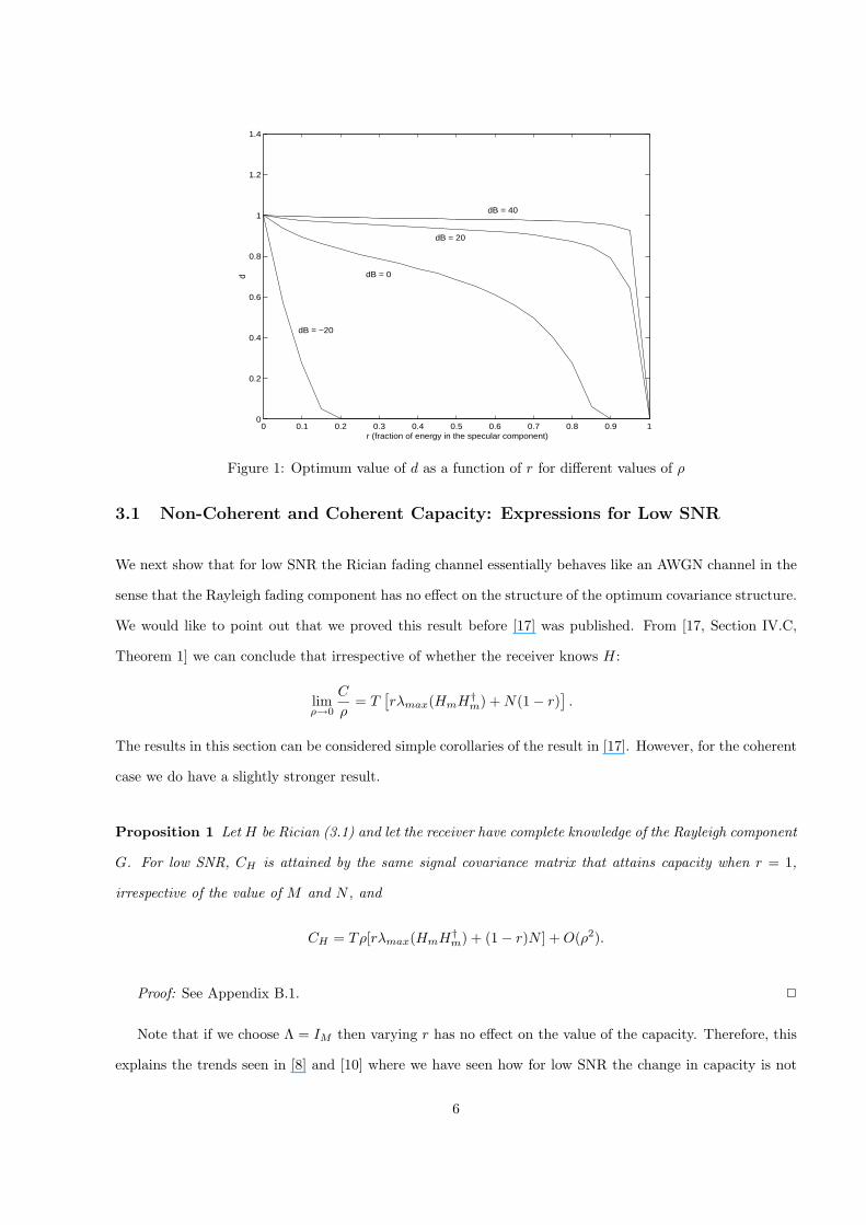
of parameters that satisfy the average power constraint (See Appendix A). Results for ρ = 100, 10, 1, 0.1 are

shown in Figure 1. As can be seen from the plot the optimum value of d stays close to 1 for high SNR and

close to 0 for low SNR. That is, the optimum covariance matrix is close to an identity matrix for high SNR.

For low SNR, all the energy is concentrated in the direction of the specular component or in other words the

optimal signaling strategy is beamforming. These observations are proven in Section 3.2.

3 General Rank Specular Component

In this case the channel matrix can be written as

H =√

1 − rG +√

rHm (3.1)

where G is the Rayleigh Fading component and Hm is a deterministic matrix such that tr{HmH†m} = MN

with no restriction on its rank. Without loss of generality, we can assume Hm to be an M × N diagonal

matrix with positive real entries.

5

0 0.1 0.2 0.3 0.4 0.5 0.6 0.7 0.8 0.9 10

0.2

0.4

0.6

0.8

1

1.2

1.4

r (fraction of energy in the specular component)

d

dB = −20

dB = 0

dB = 20

dB = 40

Figure 1: Optimum value of d as a function of r for different values of ρ

3.1 Non-Coherent and Coherent Capacity: Expressions for Low SNR

We next show that for low SNR the Rician fading channel essentially behaves like an AWGN channel in the

sense that the Rayleigh fading component has no effect on the structure of the optimum covariance structure.

We would like to point out that we proved this result before [17] was published. From [17, Section IV.C,

Theorem 1] we can conclude that irrespective of whether the receiver knows H:

limρ→0

C

ρ= T

[rλmax(HmH†

m) + N(1 − r)].

The results in this section can be considered simple corollaries of the result in [17]. However, for the coherent

case we do have a slightly stronger result.

Proposition 1 Let H be Rician (3.1) and let the receiver have complete knowledge of the Rayleigh component

G. For low SNR, CH is attained by the same signal covariance matrix that attains capacity when r = 1,

irrespective of the value of M and N , and

CH = Tρ[rλmax(HmH†m) + (1 − r)N ] + O(ρ2).

Proof: See Appendix B.1. �

Note that if we choose Λ = IM then varying r has no effect on the value of the capacity. Therefore, this

explains the trends seen in [8] and [10] where we have seen how for low SNR the change in capacity is not

6

as pronounced as for high SNR when the channel varies from a purely Rayleigh fading channel to a purely

specular one.

Proposition 2 Let H be Rician (3.1) and the receiver have no knowledge of G. For fixed M , N and T

limρ→0

C

ρ= T

[rλmax(HmH†

m) + N(1 − r)].

Proof: A more general result has been proved in [17, Theorem 1]. �

Proposition 2 suggests that at low SNR all the energy has to be concentrated in the strongest directions

of the specular component. For low SNR, we have seen that the channel behaves as an AWGN channel

in the sense that it has the same capacity as an equivalent AWGN channel Y =√

ρM SHawgn + W with

HawgnH†awgn = E[HH†]. In that respect, it would be of interest to know what the capacity would be if we

choose the source distribution to be Gaussian.

Proposition 3 Let the channel H be Rician (3.1) and the receiver have no knowledge of G. For fixed M ,

N and T if S is a Gaussian distributed source then as ρ → 0

I(X;SG) = rTρλmax(HmH†m) + O(ρ2)

where I(X;SG) is the mutual information between the output and the Gaussian source.

Proof: See Appendix B.2. �

A related version of this result appears in [12, Proposition 5.2.1].

Corollary 1 For purely Rayleigh fading channels when the receiver has no knowledge of G a Gaussian

transmitted signal satisfies limρ→0 I(X;SG)/ρ = 0.

3.2 Coherent Capacity: Expression for high SNR

For high SNR, we show that the capacity achieving signal structure basically ignores the specular component.

Theorem 2 Let H be Rician (3.1). Let CH be the capacity for H known at the receiver. As ρ → ∞, CH is

attained by an identity signal covariance matrix when M ≤ N and

CH = T · E log det[ρ

MHH†] + O(

log(√

ρ)√ρ

).

7

Proof: The expression for capacity, CH is

CH = T · E log det[IN +ρ

MH†ΛH].

Let the optimum signal covariance matrix have eigenvalues {di, i = 1, . . . , M}. We will show that di → 1 for

i = 1, . . . , M as ρ → ∞.

Let D = diag{d1, d2, . . . , dM} and H have SVD H = ΦΣΨ†. Let CΦ,Ψ,DH denote the capacity when Φ

and Ψ but not Σ are known to the transmitter and the optimum signal covariance matrix is chosen to have

eigenvalues {di} then CH ≤ CΦ,Ψ,DH . Also,

CΦ,Ψ,DH = E log det[IN +

ρ

MH†ΛΦ,ΨH]

= E log det[IN +ρ

MΣ†Φ†ΛΦ,ΨΦΣ].

Let Φ†ΛΦ,ΨΦ = DΦ. Then

log det[IN +ρ

MΣ†DΦΣ] = log det[IM +

ρ

MDΦΣΣ†].

The right hand side expression is maximized by choosing Λ such that DΦ is diagonal [3, page 255]. In other

words, we choose Λ such that DΦ = D. Let σi be the eigenvalues of ΣΣ† and define

EA[f(x)] def= E[f(x)χA(x)] (3.2)

where χA(x) is the indicator function for the set A (χA(x) = 0 if x /∈ A and χA(x) = 1 otherwise). Then for

large ρ

CΦ,Ψ,DH = E log det[IM +

ρ

MDΣΣ†]

=M∑i=1

Eσi<1/√

ρ log[1 +ρ

Mdiσi] +

M∑i=1

Eσi≥1/√

ρ log[1 +ρ

Mdiσi].

Let K denote the first term in the right hand side of the expression above and L denote the second term. It

is easy to show that

CΦ,Ψ,DH = E log det[IM +

ρ

MDΣΣ†]

= logρ

M+

M∑i=1

log(di) +M∑i=1

Eσi>1/√

ρ[log(σi)] + O(log(√

ρ)/√

ρ)

since

K ≤ log[1 +√

ρ]M∑i=1

P (σi < 1/√

ρ) = O(log(√

ρ)/√

ρ)

8

and

L = logρ

M+

M∑i=1

log(di) +M∑i=1

Eσi>1/√

ρ[log(σi)] + O(1/√

ρ).

Let CIH denote the capacity achieved when the transmission signal covariance matrix is chosen to be an

identity matrix. Then CH ≥ CIH . Also,

CIH = E log det[IN +

ρ

MH†H]

= E log det[IN +ρ

MΣ†Σ]

= E log det[IM +ρ

MΣΣ†].

Proceeding as before, we obtain

CIH = E log det[IM +

ρ

MDΣΣ†]

= logρ

M+ M log d +

M∑i=1

Eσi>1/√

ρ[log(σi)] + O(log(√

ρ)/√

ρ)

where d = 1 ⇒ M log d = 0 in the previous expression.

Since∑M

i=1 di = M and log is a convex cap function, we have∑M

i=1 log di ≤ M log d with equality only

if di = d for all i = 1, . . . , M . If we assume that the limit, as ρ →,∞ of the optimum signal covariance

matrix is not an identity matrix then we obtain a contradiction since CΦ,Ψ,DH −CI

H =∑M

i=i log di−M log d+

O(log(√

ρ)/√

ρ) can be made negative by choosing ρ to be large enough. �

For M > N , optimization using the steepest descent algorithm similar to the one described in Appendix

A shows that for high SNR the capacity achieving signal matrix is an identity matrix as well and the capacity

is given by

CH ≈ T · E log det[IN +ρ

MH†H].

3.3 Non-Coherent Capacity Upper and Lower Bounds

It follows from the data processing theorem that the non-coherent capacity, C can never be greater than the

coherent capacity CH , that is, the uninformed capacity is never decreased when the channel is known to the

receiver.

Proposition 4 Let H be Rician (3.1) and the receiver have no knowledge of the Rayleigh component. Then

C ≤ CH .

9

Now, we establish a lower bound which is similar in flavor to those derived in [8] and [10].

Proposition 5 Let H be Rician (3.1). A lower bound on capacity when the receiver has no knowledge of G

is

C ≥ CH − NE[log2 det

(IT + (1 − r)

ρ

MSS†

)](3.3)

≥ CH − NM log2(1 + (1 − r)ρ

MT ). (3.4)

Proof: Proof is similar to that of Proposition 2 in [10] and won’t be repeated here. �

We notice that the second term in the lower bound goes to zero when r = 1: as expected.

As ρ → ∞, the normalized lower bound is dominated by the following term(min{M,N} − NM

T

)log ρ.

Note that choosing M ′ < M or N ′ < N transmit antennas we get another lower bound to the capacity.

Therefore, we can improve on the lower bound above by maximing the coefficient of log ρ over the number

of transmit and receive antennas. We obtain

maxM ′≤M,N ′≤N

(min{M,N} − NM

T

)= K(1 − K

T)

where K = min{M,N, �T/2�}. Therefore, we see that the number of degrees of freedom for a non-coherent

Rician block fading channel is at least as much as that of a non-coherent Rayleigh block fading channel.

3.4 Non-Coherent Capacity: Expressions for High SNR

In this section we apply the method developed in [18] for the analysis of Rayleigh fading channels. The only

difference between the models considered in [18] and here is that we assume H has a deterministic non-zero

mean. For convenience, we use a different notation for the channel model:

X = SH + W

with H =√

rHm +√

1 − rG where Hm is the specular component of H and G denotes the Rayleigh

component. G and W consist of Gaussian circular independent random variables and the covariance matrices

of G and W are given by (1 − r)IMN and σ2ITN , respectively. Hm is a deterministic matrix satisfying

tr{HmH†m} = MN . G satisfies E[tr{GG†}] = MN and r is a number between 0 and 1 so that E[tr{HH†}] =

MN .

10

Lemma 1 Let the channel be Rician (3.1) and the receiver have no knowledge of G. Then the capacity

achieving signal, S can be written as S = ΦV Ψ† where Φ is a T × M unitary matrix independent of V and

Ψ. V and Ψ are M × M .

Proof: Follows from the fact that p(ΦX|ΦS) = p(X|S). �

In [18] the requirement for X = SH + W was that X had to satisfy the property that in the singular

value decomposition of X, X = ΦV Ψ† Φ be independent of V and Ψ. This property holds for the case

of Rician fading too because the density functions of X, SH and S are invariant to pre-multiplication by

a unitary matrix. Therefore, the leading unitary matrix in the SVD decomposition of any of X, SH and

S is independent of the other two components in the SVD and isotropically distributed. This implies that

Lemma 6 in [18] holds and we have

Lemma 2 Let R = ΦRΣRΨ†R be such that ΦR is independent of ΣR and ΨR. Then

H(R) = H(QΣRΨ†R) + log |G(T,M)| + (T − M)E[log det Σ2

R],

where Q is an M×M unitary matrix independent of V and Ψ and |G(T,M)| is the volume of the Grassmann

manifold and is equal to ∏Ti=T−M+1

2πi

(i−1)!∏Mi=1

2πi

(i−1)!

.

The Grassmann manifold G(T,M) [18] is the set of equivalence classes of all T × M unitary matrices such

that if P,Q belong to an equivalence class then P = QU for some M × M unitary matrix U .

3.4.1 M = N , T ≥ 2M

To calculate I(X;S) we need to compute H(X) and H(X|S). To compute H(X|S) we note that given S,

X is a Gaussian random vector with columns of X independent of each other. Each row has the common

covariance matrix given by (1 − r)SS† + σ2IT = ΦV 2Φ† + σ2IT . Therefore

H(X|S) = ME[M∑i=1

log(πe((1 − r)‖si‖2 + σ2)] + M(T − M) log(πeσ2).

To compute H(X), we write the SVD: X = ΦXΣXΨ†X . Note that ΦX is isotropically distributed and

independent of ΣXΨ†X , therefore from Lemma 2 we have

H(X) = H(QΣXΨ†X) + log |G(T,M)| + (T − M)E[log det Σ2

X ].

11

We first characterize the optimal input distribution in the following lemma.

Lemma 3 Let H be Rician (3.1) and the receiver have no knowledge of G. Let (sσi , i = 1, . . . , M) be the

optimal input signal of each antenna at when the noise power at the receive antennas is given by σ2. If

T ≥ 2M ,

σ

‖sσi ‖

P−→ 0, for i = 1, . . . , M (3.5)

where P−→ denotes convergence in probability.

Proof: See Appendix C. �

Lemma 4 Let H be Rician (3.1) and the receiver have no knowledge of G. The maximal rate of increase of

capacity, maxp(S):E[tr{SS†}]≤TM I(X;S) with SNR is M(T−M) log ρ and the constant norm source ‖si‖2 = T

for i = 1, . . . , M attains this rate.

Proof: See Appendix C. �

Lemma 5 Let H be Rician (3.1) and the receiver have no knowledge of G. As T → ∞ the optimal source

in Lemma 4 is the constant norm input

Proof: See Appendix C. �

From now on, we assume that the optimal input signal is the constant norm input. For the constant

norm input ΦV Ψ† = ΦV since Φ is isotropically distributed.

Theorem 3 Let the channel be Rician (3.1) and the receiver have no knowledge of G. For the constant

norm input, as σ2 → 0 the capacity is given by

C = log |G(T,M)| + (T − M)E[log detH†H] − M(T − M) log πeσ2 −

M2 log πe + H(QV H) + (T − 2M)M log T − M2 log(1 − r)

where Q, V and |G(T,M)| are as defined in Lemma 2.

Proof: Since ‖s2i ‖ � σ2 for all i = 1, . . . , M

H(X|S) = ME[M∑i=1

log πe((1 − r)‖si‖2 + σ2)] + M(T − M) log(πeσ2)

12

≈ ME[M∑i=1

log πe(1 − r)‖si‖2] + M(T − M) log πeσ2

= ME[log det(1 − r)V 2] + M2 log πe + M(T − M) log πeσ2

and from Appendix D

H(X) ≈ H(SH)

= H(QV H) + log |G(T,M)| + (T − M)E[log det(H†V 2H)]

= H(QV H) + log |G(T,M)| + (T − M)E[log detV 2] +

(T − M)E[log detHH†].

Combining the two equations

I(X;S) ≈ log |G(T,M)| + (T − M)E[log detH†H] − M(T − M) log πeσ2 +

H(QV H) − M2 log πe + (T − 2M)E[log detV 2] − M2 log(1 − r).

Now, since the optimal input signal is ‖si‖2 = T for i = 1, . . . , M , we have

C = I(X;S)

≈ log |G(T,M)| + (T − M)E[log detH†H] − M(T − M) log πeσ2 −

M2 log πe + H(QV H) + (T − 2M)M log T − M2 log(1 − r).

�

Theorem 4 Let H be Rician (3.1) and the receiver have no knowledge of G. As T → ∞ the normalized

capacity C/T → E[log det ρM H†H] where ρ = M/σ2.

Proof: First, a lower bound to capacity as σ2 → 0 is given by

C ≥ log |G(T,M)| + (T − M)E[log detH†H] + M(T − M) logTρ

Mπe−

M2 log T − M2 log(1 − r) − M2 log πe.

In [18] it’s already been shown that limT→∞( 1T log |G(T,M)|+M(1− M

T ) log Tπe ) = 0. Therefore we have

as T → ∞

C/T ≥ ME[log detρ

MH†H].

13

Second, since H(QV H) ≤ M2 log(πeT ) an asymptotic upper bound on capacity is given by

C ≤ log |G(T,M)| + (T − M)E[log detH†H] + M(T − M) logTρ

Mπe−

M2 log(1 − r).

Therefore, we have as T → ∞

C/T ≤ E[log detρ

MH†H].

�

3.4.2 M < N , T ≥ M + N

In this case we show that the optimal rate of increase is given by M(T − M) log ρ. The higher number of

receive antennas can provide only a finite increase in capacity for all SNRs.

Theorem 5 Let the channel be Rician (3.1) and the receiver have no knowledge of G. Then the maximum

rate of increase of capacity with respect to log ρ is given by M(T − M).

Proof: See Appendix C. �

For this case the lower bound on capacity tells us that the minimal rate of increase of capacity with respect

to log ρ is also M(T − M). Therefore, we conclude that the rate of increase is indeed M(T − M) log ρ.

4 Conclusions and Future Work

In this paper, we have analyzed the standard Rician fading channel for capacity. Most of the analysis was

for a general specular component but, for the special case of a rank-one specular component we were able to

show more structure on the signal input. For the case of general specular component, we were able to derive

asymptotic closed form expressions for capacity for low and high SNR scenarios.

One important result of the analysis is that for low SNRs beamforming is very desirable whereas for high

SNR scenarios it is not. This result is very useful in designing space-time codes. For high SNR scenarios,

the standard codes designed for Rayleigh fading work for the case of Rician fading as well. We conclude as

in [18] that for the case M ≤ N and T ≥ M + N the number of degrees of freedom is given by M T−MT . For

14

the general case of M , N and T , we conclude from the lower bound on capacity that the number of degrees

of freedom is atleast as much as K T−KT where K = min{M,N, �T/2�}.

A lot more work needs to be done such as for case of M > N along the lines of [18]. It also seems

reasonable that the work in [1] can be extended to the case of Rician fading.

APPENDICES

A Capacity Optimization in Section 2.1

We have the following expression for the capacity

C = E log det(IN +ρ

MH†ΛH)

where Λ is of the form

Λ =[

M − (M − 1)d 0τM−1

0M−1 dIM−1

].

We can find the optimal value of d iteratively by using the method of steepest descent as follows

dk+1 = dk + µ∂C

∂dk

where dk is the value of d at the kth iteration. We use the following identity (Jacobi’s formula) to calculate

the partial derivatives.∂ log det A

∂d= tr{A−1 ∂A

∂d}.

Therefore, we obtain

∂C

∂d= Etr{[IN +

ρ

MH†ΛH]−1 ρ

MH† ∂Λ

∂dH}

where

∂Λ∂d

=[ −(M − 1) 0τ

M−1

0M−1 IM−1

]

The derivative can be evaluated using monte carlo simulation.

15

B Non-coherent Capacity for low SNR values

B.1 Proof of Proposition 1

Proof: Let ‖H‖ denote the matrix 2-norm of H, γ be a positive number such that γ ∈ (0, 1) then

CH = T · E log det[IN +ρ

MH†ΛH]

= T · E‖H‖≥1/ργ log det[IN +ρ

MH†ΛH] + E‖H‖<1/ργ log det[IN +

ρ

MH†ΛH]

= TEtr{ ρ

MH†ΛH} + O(ρ2−2γ)

where E‖H‖≥1/ργ [·] is as defined in (3.2). This follows from the fact that P (‖H‖ ≥ 1/ργ) ≤ O(e−1

T Mργ ) and

for ‖H‖ < 1/ργ log det[IN + ρM H†ΛH] = tr[ ρ

M H†ΛH] + O(ρ2−2γ). Since γ is arbitrary

E log det[IN +ρ

MH†ΛH] = Etr[

ρ

MH†ΛH] + O(ρ2).

Now

Etr[H†ΛH] = tr{(1 − r)E[G†ΛG] + rH†mΛHm]}

= tr{(1 − r)ΛE[GG†] + rΛHmH†m}.

Therefore, we have to choose Λ to maximize tr{(1 − r)NΛ + rΛHmH†m}. Since Hm is diagonal the trace

depends only on the diagonal elements of Λ. Therefore, Λ can be chosen to be diagonal. Also, because of

the power constraint, tr{Λ} ≤ M , to maximize the expression we choose tr{Λ} = M . The maximizing Λ has

as many non-zero elements as the multiplicity of the maximum eigenvalue of (1 − r)NIM + rHmH†m. The

non-zero elements of Λ multiply the maximum eigenvalues of (1 − r)NIM + rHmH†m and can be chosen to

be of equal magnitude summing up to M . This is the same Λ maximizing the capacity for additive white

Gaussian noise channel with channel Hm. And that completes the proof. �

For the rest of this section, we introduce some new notation for ease of description. If X is a T × N

matrix then let X denote the “unwrapped” NT × 1 vector formed by placing the transposed rows of X

in a single column in an increasing manner. That is, if Xi,j denotes the element of X in the ith row and

jth column then Xi,1 = Xi/N,i%N , where �i/N� denotes the greater integer less than or equal to i/N and

i%N denotes the operation i modulo N . The channel model X =√

ρM SH + W can now be written as

X =√

ρM HS + W . H is given by H = IT ⊗Hτ where Hτ denotes the transpose of H. The notation A⊗B

denotes the Kronecker product of the matrices A and B and is defined as follows. If A is a I ×J matrix and

16

B a K × L matrix then A ⊗ B is a IK × JL matrix

A ⊗ B =

(A)11B (A)12B . . . (A)1JB(A)21B (A)22B . . . (A)2JB

......

. . ....

(A)I1B (A)I2B . . . (A)IJB

.

This way, we can describe the conditional probability density function p(X|S) as follows

p(X|S) =1

πTN |ΛX|S |e−(X−

√r ρ

M HmS)†Λ−1X|S(X−

√r ρ

M HmS)

where |ΛX|S | = det(ITN + (1 − r)SS† ⊗ IN ).

B.2 Proof of Proposition 3

First, I(X;S) = H(X) −H(X|S). Since S is Gaussian distributed, E[log det(IN + ρM HΛSH†)] ≤ H(X) ≤

log det(IN + ρM ΛX) where the expectation is taken over the distribution of H and HΛSH† = ΛX|H is

the covariance of X for a particular H. Next, we show that H(X) = ρM tr{ΛX} + O(ρ2). First, the

upper bound to H(X) can be written as ρM tr{ΛX} + O(ρ2) because H is Gaussian distributed and the

probability that ‖H‖ > R is of the order e−R2. Second, using notation (3.2) E[log det(ITN + ρ

M HΛSH†)] =

E‖H‖<( Mρ )γ [·] + E‖H‖≥( M

ρ )γ [·] where γ is a number such that 2 − γ > 1 or γ < 1. Then

E[log det(ITN +ρ

MHΛSH†)] =

ρ

ME‖H‖<( M

ρ )γ [tr{HΛSH†}] +

O(ρ2−γ) + O(log((M

ρ)γ)e−( M

ρ )γ

)

=ρ

ME[tr{HΛH†}] + O(ρ2−γ).

Since γ is arbitrary, we have H(X) = ρM E[tr{HΛSH†}] + O(ρ2). Note that ΛX = E[ΛX|H ] and since H(X)

is sandwiched between two expressions of the form ρM tr{ΛX} + O(ρ2) the assertion follows.

Now H(X|S) = E[log det(ITN + (1 − r) ρM SS† ⊗ IN )]. It can be shown similarly that H(X|S) = (1 −

r) ρM tr{E[SS† ⊗ IN ]} + O(ρ2).

Recall that H =√

rHm +√

1 − rG. Therefore, ΛX = E[HΛSH†] = rHmΛSH†m +(1−r)E[SS†]⊗IN and

we have, for a Gaussian distributed input, I(X;SG) = r ρM tr{HmΛSH†

m} + O(ρ2). Since Hm is a diagonal

matrix only the diagonal elements of ΛS matter and we we can choose the signals to be independent from

time instant to time instant. Also, to maximize tr{HmΛSH†m} under the condition tr{Λ} ≤ TM it is best

17

to concentrate all the available energy on the largest eigenvalues of Hm. Therefore, we obtain

I(X;SG) = rρ

MTMλmax(HmH†

m) + O(ρ2).

And that completes the proof.

C Proof of Lemma 3 in Section 3.4.1

In this section we will show that as σ2 → 0 or as ρ → ∞ for the optimal input (s(σ)i , i = 1, . . . , M), ∀δ, ε > 0,

∃σ0 such that for all σ < σ0

P (σ

‖sσi ‖

> δ) < ε (C.1)

for i = 1, . . . , M . s(σ)i denotes the optimum input signal being transmitted over antenna i, i = 1 . . . , M when

the noise power at the receiver is σ2. Also, throughout we use ρ to denote the average signal to noise ratio

M/σ2 present at each of the receive antennas.

The proof in this section has basically been reproduced from [18] except for some minor changes to account

for the deterministic specular component (Hm) present in the channel. The proof is by contradiction. We

need to show that if the distribution P of a source s(σ)i satisfies P ( σ

‖si‖ > δ) > ε for some ε and δ and for

arbitrarily small σ2, there exists σ2 such that s(σ)i is not optimal. That is, we can construct another input

distribution that satisfies the same power constraint, but achieves higher mutual information. The steps in

the proof are as follows

1. We show that in a system with M transmit and N receive antennas, coherence time T ≥ 2N , if

M ≤ N , there exists a finite constant k1 < ∞ such that for any fixed input distribution of S, I(X;S) ≤k1 + M(T − M) log ρ. That is, the mutual information increases with SNR at a rate no higher than

M(T − M) log ρ.

2. For a system with M transmit and receive antennas, if we choose signals with significant power only

in M ′ of the transmit antennas, that is ‖si‖ ≤ Cσ for i = M ′ + 1, . . . , M and some constant C, we

show that the mutual information increases with SNR at rate no higher than M ′(T − M ′) log ρ.

3. We show that for a system with M transmit and receive antennas if the input distribution doesn’t

satisfy (C.1), that is, has a positive probability that ‖si‖ ≤ Cσ, the mutual information achieved

increases with SNR at rate strictly lower than M(T − M) log ρ.

18

4. We show that in a system with M transmit and receive antennas for constant equal norm input

P (‖si‖ =√

T ) = 1, for i = 1, . . . , M , the mutual information increases with SNR at rate M(T −M) log ρ. Since M(T − M) ≥ M ′(T − M ′) for any M ′ ≤ M and T ≥ 2M , any input distribution that

doesn’t satisfy (C.1) yields a mutual information that increases at lower rate than constant equal norm

input, and thus is not optimal at high enough SNR level.

Step 1 For a channel with M transmit and N receive antennas, if M < N and T ≥ 2N , we write the

conditional differential entropy as

H(X|S) = N

M∑i=1

E[log((1 − r)‖si‖2 + σ2)] + N(T − M) log πeσ2.

Let X = ΦXΣXΨ†X be the SVD for X then

H(X) ≤ H(ΦX) + H(ΣX |Ψ) + H(Ψ) + E[log JT,N (σ1, . . . , σN )]

≤ H(ΦX) + H(ΣX) + H(Ψ) + E[log JT,N (σ1, . . . , σN )]

= log |R(N,N)| + log |R(T,N)| + H(ΣX) + E[log JT,N (σ1, . . . , σN )]

where R(T,N) is the Steifel manifold for T ≥ N [18] and is defined as the set of all unitary T ×N matrices.

|R(T,N)| is given by

|R(T,N)| =T∏

i=T−N+1

2πi

(i − 1)!.

JT,N (σ1, . . . , σN ) is the Jacobian of the transformation X → ΦXΣXΨ†X [18] and is given by

JT,N = (12π

)N∏

i<j≤N

(σ2i − σ2

j )2N∏

i=1

σ2(T−M)+1i .

We have also chosen to arrange σi in decreasing order so that σi > σj if i < j. Now

H(ΣX) = H(σ1, . . . , σM , σM+1, . . . , σN )

≤ H(σ1, . . . , σM ) + H(σM+1, . . . , σN )

Also,

E[log JT,N (σ1, . . . , σN )] = log1

(2π)N+

N∑i=1

E[log σ2(T−N)+1i ] +

∑i<j≤N

E[log(σ2i − σ2

j )2]

= log1

(2π)M+

M∑i=1

E[log σ2(T−N)+1i ] +

∑i<j≤M

E[log(σ2i − σ2

j )2] +∑

i≤M,M<j≤N

E[log(σ2i − σ2

j )2︸ ︷︷ ︸≤log σ4

i

] +

19

log1

(2π)N−M+

N∑i=M+1

E[log σ2(T−N)+1i ] +

∑M<i<j≤N

E[log(σ2i − σ2

j )2]

≤ E[log JN,M (σ1, . . . , σM )]

+E[log JT−M,N−M (σM+1, . . . , σN )]

+2(T − M)M∑i=1

E[log σ2i ].

Next define C1 = Φ1Σ1Ψ†1 where Σ1 = diag(σ1, . . . , σM ), Φ1 is a N ×M unitary matrix, Ψ1 is a M ×M

unitary matrix. Choose Σ1, Φ1 and Ψ1 to be independent of each other. Similarly define C2 from the rest

of the eigenvalues. Now

H(C1) = log |R(M,M)| + log |R(N,M)| + H(σ1, . . . , σM ) + E[log JN,M (σ1, . . . , σM )]

H(C2) = log |R(N − M,N − M)| + log |R(T − M,N − M)|

+H(σM+1, . . . , σN ) + E[log JT−M,N−M (σM+1, . . . , σN )].

Substituting in the formula for H(X), we obtain

H(X) ≤ H(C1) + H(C2) + (T − M)M∑i=1

E[log σ2i ] + log |R(T,N)| + log |R(N,N)|

− log |R(N,M)| − log |R(M,M)| − log |R(N − M,N − M)| −

log |R(T − M,N − M)|

= H(C1) + H(C2) + (T − M)M∑i=1

E[log σ2i ] + log |G(T,M)|.

Note that C1 has bounded total power

tr{E[C1C†1 ]} = tr{E[σ2

i ]} = tr{E[XX†]} ≤ NT (M + σ2).

Therefore, the differential entropy of C1 is bounded by the entropy of a random matrix with entries iid

Gaussian distributed with variance T (M+σ2)M [3, p. 234, Theorem 9.6.5]. That is

H(C1) ≤ NM log[πe

T (M + σ2)M

].

Similarly, we bound the total power of C2. Since σM+1, . . . , σN are the N − M least singular values of X,

for any (N − M) × N unitary matrix Q.

tr{E[C2C†2 ]} ≤ (N − M)Tσ2.

20

Therefore, the differential entropy is maximized if C2 has independent iid Gaussian entries and

H(C2) ≤ (N − M)(T − M) log[πe

Tσ2

T − M

].

Therefore, we obtain

H(X) ≤ log |G(T,M)| + NM log[πe

T (M + σ2)M

]+ (T − M)

M∑i=1

E[log σ2i ]

+(N − M)(T − M) log πeσ2 + (N − M)(T − M) logT

T − M.

Combining with H(X|S), we obtain

I(X;S) ≤ log |G(T,M)| + NM logT (M + σ2)

M+ (N − M)(T − M) log

T

T − M︸ ︷︷ ︸α

+ (T − M − N)M∑i=1

E[log σ2i ]

︸ ︷︷ ︸β

+

N

(M∑i=1

E[log σ2i ] −

M∑i=1

E[log((1 − r)‖si‖2 + σ2)]

)︸ ︷︷ ︸

γ

−M(T − M) log πeσ2.

By Jensen’s inequality

M∑i=1

E[log σ2i ] ≤ M log(

1M

M∑i=1

E[σ2i ])

= M logNT (M + σ2)

M.

For γ it will be shown that

M∑i=1

E[log σ2i ] −

M∑i=1

E[log((1 − r)‖si‖2 + σ2)] ≤ k

where k is some finite constant.

Given S, X has mean√

rSHm and covariance matrix IN ⊗ ((1 − r)SS† + σ2IT ). If S = ΦV Ψ† then

X†X = H†S†SH + W †SH + H†S†W + W †W

d= H†1V †V H1 + W †V †H1 + H†

1V W + W †W

where H1 has the covariance matrix as H but mean is given by√

rΨ†Hm. Therefore, X†X = X†1X1 where

X1 = V H1 + W

21

Now, X1 has the same distribution as ((1 − r)V V † + σ2IT )1/2Z where Z is a random Gaussian matrix

with mean√

r((1 − r)V V † + σ2IT )−1/2Ψ†Hm and covariance INT . Therefore,

X†X d= Z†((1 − r)V V † + σ2IT )Z.

Let (X†X|S) denote the realization of X†X given S then

(X†X|S) d= Z†

(1 − r)‖s1‖2 + σ2

. . .(1 − r)‖sM‖2 + σ2

σ2

. . .σ2

Z.

Let Z = [Z1|Z2] be the partition of Z such that

(X†X|S) d= Z†1((1 − r)V 2 + σ2IM )Z1 + σ2Z†

2Z2

where Z1 has mean√

r((1−r)V 2+σ2IM )−1/2V Ψ†Hm and covariance INM and Z2 has mean 0 and covariance

IN(T−M)

We use the following Lemma from [11]

Lemma 6 If C and B are both Hermitian matrices, and if their eigenvalues are both arranged in decreasing

order, thenN∑

i=1

(λi(C) − λi(B))2 ≤ ‖C − B‖22

where ‖A‖22

def=∑

A2ij, λi(A) denotes the ith eigenvalue of Hermitian matrix A.

Applying this Lemma with C = (X†X|S) and B = Z†1(V 2 + σ2IM )Z1 we obtain

λi(C) ≤ λi(B) + σ2‖Z†2Z2‖2

for i = 1, . . . , M Note that λi(B) = λi(B′) where B′ = ((1 − r)V 2 + σ2IM )Z1Z†1 . Let k = E[‖Z†

2Z2‖2] be a

finite constant. Now, since Z1 and Z2 are independent matrices (covariance of [Z1|Z2] is a diagonal matrix)M∑i=1

E[log σ2i |S] ≤

M∑i=1

E[log(λi(((1 − r)V 2 + σ2IM )Z1Z†1) + σ2‖Z†

2Z2‖2)]

=M∑i=1

E[E[log(λi(((1 − r)V 2 + σ2IM )Z1Z†1) + σ2‖Z†

2Z2‖2) | Z1]]

≤M∑i=1

E[log(λi(((1 − r)V 2 + σ2IM )Z1Z†1) + σ2k)]

= E[log det(((1 − r)V 2 + σ2IM )Z1Z†1 + kσ2IM )]

= E[log detZ1Z†1 ] + E[log det((1 − r)V 2 + σ2IM + kσ2(Z1Z

†1)−1)]

22

where the second inequality follows from Jensen’s inequality and taking expectation over Z2. Using Lemma

6 again on the second term, we have

M∑i=1

E[log σ2i |S] ≤ E[log detZ1Z

†1 ] + E[log det((1 − r)V 2 + σ2IM

+kσ2‖(Z1Z1)−1‖2IM )]

≤ E[log detZ1Z†1 ] + E[log det((1 − r)V 2 + k′σ2IM )]

where k′ = 1 + kE[‖Z1Z†1‖2] is a finite constant. Next, we have

M∑i=1

E[log σ2i |S] −

M∑i=1

log((1 − r)‖si‖2 + σ2) ≤ E[log detZ1Z†1 ] +

M∑i=1

log(1 − r)‖si‖2 + k′σ2

(1 − r)‖si‖2 + σ2

≤ E[log detZ1Z†1 ] + k′′

where k′′ is another constant. Taking Expectation over S, we have shown that∑M

i=1 E[log σ2i ]−∑M

i=1 E[log((1−r)‖si‖2 + σ2)] is bounded above by a constant.

Note that as ‖si‖ → ∞, Z1 →√

11−r H1 so that E[Z1Z

†1 ] → 1

1−r E[H1H†1 ] = 1

1−r E[HH†].

Step 2 Now assume that there are M transmit and receive antennas and that for N −M ′ > 0 antennas,

the transmitted signal has bounded energy, that is, ‖si‖2 < Cσ2 for some constant C. Start from a system

with only M ′ transmit antennas, the extra power we send on the rest M − M ′ antennas accrues only a

limited capacity gain since the SNR is bounded. Therefore, we conclude that the mutual information must

be no more than k2 + M ′(T − M ′) log ρ for some finite k2 that is uniform for all SNR level and all input

distributions.

Particularly, if M ′ = M − 1, ie we have at least 1 transmit antenna to transmit signal with finite SNR,

under the assumption that T ≥ 2M (T greater than twice the number of receivers), we have M ′(T −M ′) <

M(T − M). This means that the mutual information achieved has an upper bound that increases with log

SNR at rate M ′(T − M ′) log ρ, which is a lower rate than M(T − M) log ρ.

Step 3 Now we further generalize the result above to consider the input which on at least 1 antennas,

the signal transmitted has finite SNR with a positive probability, that is P (‖sM‖2 < Cσ2) = ε. Define the

event E = {‖sM‖2 < Cσ2}, then the mutual information can be written as

I(X;S) ≤ εI(X;S|E) + (1 − ε)I(X;S|Ec) + I(E;X)

≤ ε(k1 + (M − 1)(T − M + 1) log ρ) + (1 − ε)(k2 + M(T − M) log ρ) + log 2

23

where k1 and k2 are two finite constants. Under the assumption that T ≥ 2M , the resulting mutual

information thus increases with SNR at rate that is strictly less than M(T − M) log ρ.

Step 4 Here we will show that for the case of M transmit and receive antennas, the constant equal

norm input P (‖si‖ =√

T ) = 1 for i = 1, . . . , M , achieves a mutual information that increases at a rate

M(T − M log ρ.

Lemma 7 For the constant equal norm input,

lim infσ2→0

[I(X;S) − f(ρ)] ≥ 0

where ρ = M/σ2, and

f(ρ) = log |G(T,M)| + (T − M)E[log detHH†] + M(T − M) logTρ

Mπe− M2 log[(1 − r)T ]

where |G(T,M)| is as defined in Lemma 2.

Proof: Consider

H(X) ≥ H(SH)

= H(QV H) + log |G(T,M)| + (T − M)E[log detH†ΨV 2Ψ†H]

= H(QV H) + log |G(T,M)| + M(T − M) log T + (T − M)E[log detHH†]

H(X|S) ≤ H(QV H) + MM∑i=1

E[log((1 − r)‖si‖2 + σ2)] + M(T − M) log πeσ2

≈ H(QV H) + M2 log[(1 − r)T ] + M2 σ2

(1 − r)T+ M(T − M) log πeσ2.

Therefore,

I(X;S) ≥ log |G(T,M)| + (T − M)E[log detHH†] − M(T − M) log πeσ2 +

M(T − M) log T − M2 log[(1 − r)T ] − M2 σ2

(1 − r)T

= f(ρ) − M2 σ2

(1 − r)T→ f(ρ).

�

Combining the result in step 4 with results in Step 3 we see that for any input that doesn’t satisfy (C.1)

the mutual information increases at a strictly lower rate than for the equal norm input. Thus at high SNR,

any input not satisfying (C.1) is not optimal and this completes the proof of Lemma 3.

24

D Convergence of H(X) for T > M = N

The results in this section are needed in the proof of Theorem 3 in Section 3.4.1. We need the following two

theorems, proved in [9], for proving the results in this section.

Theorem 6 Let {Xi ∈ Cl P } be a sequence of continuous random variables with probability density functions,

{fi} and X ∈ Cl P be a continuous random variable with probability density function f such that fi → f

pointwise. If 1) max{fi(x), f(x)} ≤ A < ∞ for all i and 2) max{∫ ‖x‖κfi(x)dx,∫ ‖x‖κf(x)dx} ≤ L < ∞

for some κ > 1 and all i then H(Xi) → H(X). ‖x‖ =√

x†x denotes the Euclidean norm of x.

Theorem 7 Let {Xi ∈ Cl P } be a sequence of continuous random variables with probability density functions,

fi and X ∈ Cl P be a continuous random variable with probability density function f . Let XiP−→ X.

If 1)∫ ‖x‖κfn(x)dx ≤ L and

∫ ‖x‖κf(x)dx ≤ L for some κ > 1 and L < ∞ 2) f(x) is bounded then

lim supi→∞ H(Xi) ≤ H(X).

First, we will show convergence for the case T = M = N needed for Theorem 3 and then use the result

to show convergence for the general case of T > M = N . We need the following lemma to establish the

result for T = M = N .

Lemma 8 If λmin(SS†) ≥ λ > 0 then ∀n there exists an M such that |f(X)− f(Z)| < Mδ if |X −Z| < δ.

Proof: Let Z = X + ∆X with |∆X| < δ and [σ2IT + (1 − r)SS†] = D. First, we will fix S and show

that for all S, f(X|S) satisfies the above property. Therefore, it will follow that f(X) also satisfies the same

property. Consider f0(X|S) the density defined with zero mean which is just a translated version of f(X|S).

f(X + ∆X|S) = f(X|S)[1 − tr[D−1(∆XX† + X∆X† + O(‖∆X‖22))]]

then

|f(X + ∆X|S) − f(X|S)| ≤ f(X|S)|tr[D−1(∆XX† + X∆X†)] + tr[D−1‖∆X‖22]|.

Now

f(X|S) ≤ 1πTN detN [D]

· min{ 1√tr[D−1XX†]

, 1}.

25

Next, make use of the following inequalities

tr{D−1XX†} ≥ tr{λmin(D−1)XX†}

≥ λmin(D−1)λmax(XX†) = λmin(D−1)‖X‖22.

Also,

|tr{D−1(X∆X† + ∆XX† + O(‖∆X‖22)}| ≤

∑i

|λi(D−1[∆XX† + X∆X†])| +

‖D−1‖2‖∆X‖22

≤ T‖D−1‖2‖X‖2‖∆X‖2 +

T‖D−1‖2‖∆X‖22.

Therefore,

|f(X + ∆X|S) − f(X|S)| ≤ 1πTN detN [D]

· min{ 1√λmin(D−1)‖X‖2

, 1} ·

T‖D−1‖2‖∆X‖2(‖X‖2 + ‖∆X‖2).

Since, we have restricted λmin(SS†) ≥ λ > 0 we have for some constant M

|f(X + ∆X|S) − f(X|S)| ≤ M‖∆X‖2.

From which the Lemma follows. Note that det[D] compensates for√

λmin(D−1) in the denominator. �

Let’s consider the T × N random matrix X = SH + W . The entries of M × N matrix H, T = M = N ,

are independent circular complex Normal random variables with non-zero mean and unit variance whereas

the entries of W are independent circular complex Normal random variables with zero-mean and variance

σ2.

Let S be a random matrix such that λmin(SS†) ≥ λ > 0 with distribution, Fmax(S) chosen in such a

way to maximize I(X;S). For each value of σ2 = 1/n, n an integer → ∞, the density of X is

f(X) = ES

[e−tr{[σ2IT +(1−r)SS†]−1(X−√

rNMSHm)(X−√rNMSHm)†}

πTNdetN [σ2IT + (1 − r)SS†]

].

where the expectation is over Fmax(S). It is easy to see that f(X) as a function of σ2 is a continuous function

of σ2. As limσ2→0 f(X) exists, let’s call this limit g(X).

Since we have imposed the condition that λmin(SS†) ≥ λ > 0 w.p. 1, f(X) is bounded above by 1(λπ)T N .

Thus f(X) satisfies the condition for Theorem 6. From Lemma 8 we also have that for all n there exists a

26

common δ such that |f(X)− f(Z)| < ε for all |X −Z| < δ. Therefore, H(X) → Hg. Since λ is arbitrary we

conclude that for all optimal signals with the restriction λmin(SS†) > 0, H(X) → Hg. Now, we claim that

the condition λmin > 0 covers all optimal signals. Otherwise, if λmin(SS†) = 0 with finite probability then

for all σ2 we have min ‖si‖2 ≤ Lσ2 for some constant L with finite probability. This is a contradiction of

the condition (3.5). This completes the proof of convergence of H(X) for T = M = N . �

Now, we show convergence of H(X) for T > M = N . We will show that H(X) ≈ H(SH) for small values

of σ where S = ΦV Ψ† with Φ independent of V and Ψ.

Let S0 = Φ0V0Ψ†0 denote a signal with its density set to the limiting optimal density of S as σ2 → 0.

H(X) ≥ H(Y ) = H(QΣY Ψ†Y ) + log |G(T,M)| + (T − M)E[log det Σ2

Y ]

where Y = SH and Q is an isotropic matrix of size N × M . Let

YQ = QV Ψ†H

Then H(QΣY Ψ†Y ) = H(YQ).

From the proof of the case T = M = N , we have limσ2→0 H(YQ) = H(QV0Ψ†0H). Also,

limσ2→0

E[log det Σ2Y ] = E[log det Σ2

Y0]

where Y0 = S0H Therefore, lim infσ2→0 H(X) ≥ limσ2→0 H(Y ) = H(S0H).

Now, to show limσ2→0 H(X) ≤ H(S0H). From before

H(X) = H(QΣXΨ†X) + |G(T,N)| + (T − M)E[log det Σ2

X ].

Now QΣXΨ†X converges in distribution to QV0Ψ

†0H. Since the density of QV0Ψ

†0H is bounded, from

Theorem 7 we have lim supσ2→0 H(QΣXΨ†X) ≤ H(QV0Ψ

†0H). Also, note that limσ2→0 E[log det Σ2

X ] =

E[log det Σ2Y0

] = limσ2→0 E[log det Σ2Y ]. Which leads to lim supσ2→0 H(X) ≤ H(S0H) = limσ2→0 H(SH).

Therefore, limσ2→0 H(X) = limσ2→0 H(SH) and for small σ2, H(X) ≈ H(SH).

References

[1] I. Abou-Faycal and B. Hochwald, “Coding requirements for multiple-antenna channels with unknown

Rayleigh fading,” Bell Labs Technical Memorandum, Mar. 1999.

27

[2] N. Benvenuto, P. Bisaglia, A. Salloum, and L. Tomba, “Worst case equalizer for noncoherent HIPERLAN

receivers,” IEEE Trans. on Communications, vol. 48, no. 1, pp. 28–36, January 2000.

[3] T. M. Cover and J. A. Thomas, Elements of Information Theory, Wiley Series in Telecommunications,

1995.

[4] P. F. Driessen and G. J. Foschini, “On the capacity formula for multiple input-multiple output wireless

channels: A geometric interpretation,” IEEE Trans. on Communications, vol. 47, no. 2, pp. 173–176,

February 1999.

[5] F. R. Farrokhi, G. J. Foschini, A. Lozano, and R. A. Valenzuela, “Link-optimal space-time processing

with multiple transmit and receive antennas,” IEEE Communication Letters, vol. 5, no. 3, pp. 85–87,

Mar 2001.

[6] G. J. Foschini, “Layered space-time architecture for wireless communication in a fading environment

when using multiple antennas,” Bell Labs Technical Journal, vol. 1, no. 2, pp. 41–59, 1996.

[7] G. J. Foschini and M. J. Gans, “On limits of wireless communications in a fading environment when

using multiple antennas,” Wireless Personal Communications, vol. 6, no. 3, pp. 311–335, March 1998.

[8] M. Godavarti, A. O. Hero, and T. Marzetta, “Min-capacity of a multiple-antenna wireless channel in a

static Rician fading environment,” Submitted to IEEE Trans. on Wireless Communications, 2001.

[9] M. Godavarti and A. O. Hero-III, “Convergence of differential entropies,” Submitted to IEEE Trans. on

Information Theory, 2001.

[10] M. Godavarti, T. Marzetta, and S. S. Shitz, “Capacity of a mobile multiple-antenna wireless link with

isotropically random Rician fading,” Accepted for publication - IEEE Trans. on Information Theory,

2001.

[11] R. A. Horn and C. R. Johnson, Matrix Analysis, Cambridge University Press, 1996.

[12] A. Lapidoth and S. S. (Shitz), “Fading channels: How perfect need “perfect side information” be?,”

IEEE Trans. on Inform. Theory, vol. 48, no. 5, pp. 1118–1134, May 2002.

[13] T. L. Marzetta and B. M. Hochwald, “Capacity of a mobile multiple-antenna communication link in

Rayleigh flat fading channel,” IEEE Trans. on Inform. Theory, vol. 45, no. 1, pp. 139–157, Jan 1999.

[14] S. Rice, “Mathematical analysis of random noise,” Bell Systems Technical Journal, vol. 23, , 1944.

28

[15] V. Tarokh, N. Seshadri, and A. R. Calderbank, “Space-time codes for high data rate wireless commu-

nication: Performance criterion and code construction,” IEEE Trans. on Communications, vol. 44, no.

2, pp. 744–765, March 1998.

[16] I. E. Telatar, “Capacity of multi-antenna Gaussian channels,” European Transactions on Telecommu-

nications, vol. 10, no. 6, pp. 585–596, Nov/Dec 1999.

[17] S. Verdu, “Spectral efficiency in the wideband regime,” IEEE Trans. on Inform. Theory, vol. 48, no. 6,

pp. 1319–1343, June 2002.

[18] L. Zheng and D. N. C. Tse, “Packing spheres in the Grassmann manifold: A geometric approach to the

non-coherent multi-antenna channel,” IEEE Trans. on Inform. Theory, vol. 48, no. 2, pp. 359–383, Feb

2002.

29