Performance of deterministic learning in noisy environments
11
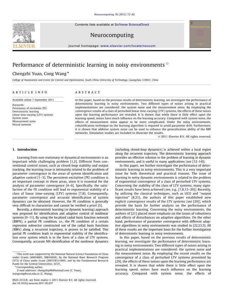
Performance of deterministic learning in noisy environments $ Chengzhi Yuan, Cong Wang n College of Automation and Center for Control and Optimization, South China University of Technology, Guangzhou 510641, China article info Available online 7 September 2011 Keywords: Persistency of excitation (PE) Deterministic learning Linear time-varying (LTV) systems System noise Measurement noise Neural network abstract In this paper, based on the previous results of deterministic learning, we investigate the performance of deterministic learning in noisy environments. Two different types of noises arising in practical implementations are considered: the system noise and the measurement noise. By employing the convergence results of a class of perturbed linear time-varying (LTV) systems, the effects of these noises upon the learning performance are revealed. It is shown that while there is little effect upon the learning speed, noises have much influence on the learning accuracy. Compared with system noise, the effects of measurement noise appear to be more complicated. Under the noisy environments, robustification technique on the learning algorithm is required to avoid parameter drift. Furthermore, it is shown that additive system noise can be used to enhance the generalization ability of the RBF networks. Simulation studies are included to illustrate the results. & 2011 Elsevier B.V. All rights reserved. 1. Introduction Learning from non-stationary or dynamical environments is an important while challenging problem [1,2]. Different from con- ventional control issues, such as closed-loop stability and output tracking, the learning issue is intimately related to the problem of parameter convergence in the areas of system identification and adaptive control [1–3]. The persistent excitation (PE) condition is an important concept in these areas, since it is essential for the analysis of parameter convergence [4–6]. Specifically, the satis- faction of the PE condition will lead to exponential stability of a class of linear time-varying (LTV) systems [7,8]. Consequently, parameter convergence and accurate identification of system dynamics can be obtained. However, the PE condition is generally very difficult to characterize and cannot be verified a priori [5]. Recently, a deterministic learning (or dynamic learning) approach was proposed for identification and adaptive control of nonlinear systems [9–11]. By using the localized radial basis function network (RBFN), a partial PE condition, i.e., the PE condition of a certain regression subvector constructed out of the radial basis functions (RBFs) along a recurrent trajectory, is proven to be satisfied. This partial PE condition leads to exponential stability of the identifica- tion error system which is in the form of a class of LTV systems. Consequently, accurate NN identification of the nonlinear dynamics (including closed-loop dynamics) is achieved within a local region along the recurrent trajectory. The deterministic learning approach provides an effective solution to the problem of learning in dynamic environments, and is useful in many applications (see [12–14]). In this paper, we further investigate the performance of deter- ministic learning in noisy environments. This is a very important issue for both theoretical and practical reasons. The issue of learning in noisy dynamic environments is related to the problem of exponential convergence of a class of perturbed LTV systems. Concerning the stability of the class of LTV systems, many signi- ficant results have been achieved (see, e.g., [7,8,15–20]). Recently, by utilizing the classical techniques, such as UCO and ‘‘output injection’’ [8,21], the authors of this paper established new explicit convergence results of the LTV systems (see [29]), which provide the basis for further analysis on the performance of deterministic learning. Concerning the noisy environments, the authors of [21] placed more emphasis on the issues of robustness and effects of disturbances on adaptive algorithms. On the other hand, performance of parameter convergence with different adap- tive algorithms in noisy environments was studied in [22,23,5]. All of these results are the important basis for the further investigation of deterministic learning in noisy environments. In this paper, based on the previous results of deterministic learning, we investigate the performance of deterministic learn- ing in noisy environments. Two different types of noises arising in practical implementations are considered: the system noise and the measurement noise. By employing the recent results on the convergence of a class of perturbed LTV systems presented by [29], the effects of these noises upon the learning performance are revealed. It is shown that while there is little effect upon the learning speed, noises have much influence on the learning accuracy. Compared with system noise, the effects of Contents lists available at SciVerse ScienceDirect journal homepage: www.elsevier.com/locate/neucom Neurocomputing 0925-2312/$ - see front matter & 2011 Elsevier B.V. All rights reserved. doi:10.1016/j.neucom.2011.05.037 $ This work was supported by the National Natural Science Foundation of China under Grants (60934001, 90816028), by the National Basic Research Program (973) of China under Grant (2007CB311005), and by the Fundamental Research Funds for the Central Universities, SCUT. n Corresponding author. E-mail addresses: [email protected] (C. Yuan), [email protected] (C. Wang). Neurocomputing 78 (2012) 72–82
Transcript of Performance of deterministic learning in noisy environments
Neurocomputing 78 (2012) 72–82
Contents lists available at SciVerse ScienceDirect
Neurocomputing
0925-23
doi:10.1
$This
under G
(973) o
Funds fn Corr
E-m
wangco
journal homepage: www.elsevier.com/locate/neucom
Performance of deterministic learning in noisy environments$
Chengzhi Yuan, Cong Wang n
College of Automation and Center for Control and Optimization, South China University of Technology, Guangzhou 510641, China
a r t i c l e i n f o
Available online 7 September 2011
Keywords:
Persistency of excitation (PE)
Deterministic learning
Linear time-varying (LTV) systems
System noise
Measurement noise
Neural network
12/$ - see front matter & 2011 Elsevier B.V. A
016/j.neucom.2011.05.037
work was supported by the National Natural
rants (60934001, 90816028), by the Natio
f China under Grant (2007CB311005), and b
or the Central Universities, SCUT.
esponding author.
ail addresses: [email protected] (C. Y
[email protected] (C. Wang).
a b s t r a c t
In this paper, based on the previous results of deterministic learning, we investigate the performance of
deterministic learning in noisy environments. Two different types of noises arising in practical
implementations are considered: the system noise and the measurement noise. By employing the
convergence results of a class of perturbed linear time-varying (LTV) systems, the effects of these noises
upon the learning performance are revealed. It is shown that while there is little effect upon the
learning speed, noises have much influence on the learning accuracy. Compared with system noise, the
effects of measurement noise appear to be more complicated. Under the noisy environments,
robustification technique on the learning algorithm is required to avoid parameter drift. Furthermore,
it is shown that additive system noise can be used to enhance the generalization ability of the RBF
networks. Simulation studies are included to illustrate the results.
& 2011 Elsevier B.V. All rights reserved.
1. Introduction
Learning from non-stationary or dynamical environments is animportant while challenging problem [1,2]. Different from con-ventional control issues, such as closed-loop stability and outputtracking, the learning issue is intimately related to the problem ofparameter convergence in the areas of system identification andadaptive control [1–3]. The persistent excitation (PE) condition isan important concept in these areas, since it is essential for theanalysis of parameter convergence [4–6]. Specifically, the satis-faction of the PE condition will lead to exponential stability of aclass of linear time-varying (LTV) systems [7,8]. Consequently,parameter convergence and accurate identification of systemdynamics can be obtained. However, the PE condition is generallyvery difficult to characterize and cannot be verified a priori [5].
Recently, a deterministic learning (or dynamic learning) approachwas proposed for identification and adaptive control of nonlinearsystems [9–11]. By using the localized radial basis function network(RBFN), a partial PE condition, i.e., the PE condition of a certainregression subvector constructed out of the radial basis functions(RBFs) along a recurrent trajectory, is proven to be satisfied. Thispartial PE condition leads to exponential stability of the identifica-tion error system which is in the form of a class of LTV systems.Consequently, accurate NN identification of the nonlinear dynamics
ll rights reserved.
Science Foundation of China
nal Basic Research Program
y the Fundamental Research
uan),
(including closed-loop dynamics) is achieved within a local regionalong the recurrent trajectory. The deterministic learning approachprovides an effective solution to the problem of learning in dynamicenvironments, and is useful in many applications (see [12–14]).
In this paper, we further investigate the performance of deter-ministic learning in noisy environments. This is a very importantissue for both theoretical and practical reasons. The issue oflearning in noisy dynamic environments is related to the problemof exponential convergence of a class of perturbed LTV systems.Concerning the stability of the class of LTV systems, many signi-ficant results have been achieved (see, e.g., [7,8,15–20]). Recently,by utilizing the classical techniques, such as UCO and ‘‘outputinjection’’ [8,21], the authors of this paper established newexplicit convergence results of the LTV systems (see [29]), whichprovide the basis for further analysis on the performance ofdeterministic learning. Concerning the noisy environments, theauthors of [21] placed more emphasis on the issues of robustnessand effects of disturbances on adaptive algorithms. On the otherhand, performance of parameter convergence with different adap-tive algorithms in noisy environments was studied in [22,23,5]. Allof these results are the important basis for the further investigationof deterministic learning in noisy environments.
In this paper, based on the previous results of deterministiclearning, we investigate the performance of deterministic learn-ing in noisy environments. Two different types of noises arising inpractical implementations are considered: the system noise andthe measurement noise. By employing the recent results on theconvergence of a class of perturbed LTV systems presented by[29], the effects of these noises upon the learning performance arerevealed. It is shown that while there is little effect upon thelearning speed, noises have much influence on the learningaccuracy. Compared with system noise, the effects of

C. Yuan, C. Wang / Neurocomputing 78 (2012) 72–82 73
measurement noise appear to be more complicated. Under thenoisy environments, robustification technique on the learningalgorithm is required to avoid parameter drift. Furthermore, it isshown that additive system noise can be used to enhance thegeneralization ability of the RBF networks.
The rest of the paper is organized as follows. Preliminary resultsand problem formulation are contained in Section 2. Effects of noisesupon the performance of deterministic learning are analyzed inSection 3. Numerical simulations to illustrate the results are given inSection 4. Section 5 concludes the paper.
2. Preliminaries and problem formulation
2.1. Localized RBF networks and PE
The RBF networks can be described by fnnðZÞ ¼PN
i ¼ 1 wisiðZÞ ¼
WT SðZÞ [24], where ZAOZ � Rq is the input vector, W ¼ ½w1, . . . ,wN �T
ARN is the weight vector, N is the NN node number, andSðZÞ ¼ ½s1ðJZ�x1JÞ, . . . ,sNðJZ�xNJÞ�
T , with sið�Þ being a radial basisfunction, and xi (i¼ 1, . . . ,N) being distinct points in state space.The Gaussian function siðJZ�xiJÞ ¼ exp½�ðZ�xiÞ
TðZ�xiÞ=Z2
i � isone of the most commonly used radial basis functions, wherexi ¼ ½xi1,xi2, . . . ,xiq�
T is the center of the receptive field and Zi is thewidth of the receptive field. The Gaussian function belongs to theclass of RBFs in the sense that siðJZ�xiJÞ-0 as JZJ-1.
It has been shown in [25] that for any continuous function f ðZÞ :OZ-R where OZ � Rq is a compact set, and for the NN approximator,where the node number N is sufficiently large, there exists an idealconstant weight vector Wn, such that for each en40, f ðZÞ ¼
WnT SðZÞþe,8ZAOZ , where 9e9oen is the approximation error.Moreover, for any bounded trajectory Z(t) within the compact setOZ , f(Z) can be approximated by using a limited number of neuronslocated in a local region along the trajectory: f ðZÞ ¼WnT
z SzðZÞþez,where subscript ð�Þz stands for the regions close to the trajectory Z(t),SzðZÞ ¼ ½sj1
ðZÞ, . . . ,sjz ðZÞ�T ARNz , with Nz oN, 9sji
94i ðji ¼ j1, . . . ,jzÞ,i40 is a small positive constant, Wn
z ¼ ½wn
j1, . . . ,wn
jz�T , and ez is the
approximation error, with ez ¼O ðeÞ ¼ OðenÞ.Based on the previous results on the PE property of RBF
networks [26,27,5], it is shown in [11] that for a localized RBFnetwork WT SðZÞ whose centers are placed on a regular lattice,almost any recurrent trajectory Z(t) can lead to the satisfaction ofthe PE condition of the regressor subvector SzðZÞ.
2.2. Deterministic learning
In deterministic learning, identification of system dynamics ofgeneral nonlinear systems is achieved according to the followingelements: (i) employment of localized RBF networks; (ii) satisfac-tion of a partial PE condition; (iii) exponential stability of theadaptive system along the periodic or recurrent orbit; (iv) locallyaccurate NN approximation of the unknown system dynamics [11].
Consider a general nonlinear dynamical system:
_x ¼ Fðx;pÞ, xðt0Þ ¼ x0 ð1Þ
where x¼ ½x1, . . . ,xn�T ARn is the state of the system, which is
measurable, p is a system parameter vector, Fðx; pÞ ¼ ½f1ðx; pÞ, . . . ,fnðx;pÞ�
T is a smooth but unknown nonlinear vector field. It isassumed that the system trajectory generated from the abovedynamical system, denoted as jzðt,x0,pÞ or jzx for simplicity ofpresentation, is a recurrent trajectory.1
1 Roughly, a recurrent trajectory is characterized as follows: given n40, there
exists a finite TðnÞ40 such that the trajectory returns to the n-neighborhood of
any point on the trajectory within a time not greater than TðnÞ. (Refer to [28] for a
rigorous definition of recurrent trajectory.)
Consider the following dynamical RBF network for identifica-tion of the unknown system dynamics Fðx; pÞ:
_x i ¼�aiðxi�xiÞþWT
i SiðxÞ, i¼ 1, . . . ,n ð2Þ
where x ¼ ½x1, . . . ,xn�T is the state vector, x is the state of system
(1), ai40 is the design constant, and WT
i SiðxÞ is a RBF networkused to approximate the unknown nonlinearity fiðx; pÞ of (1). Theweight estimates W i in (2) are updated by using the followingLyapunov-based learning law:
_W i ¼�GiSiðxÞ ~xi�siGiW i, i¼ 1, . . . ,n ð3Þ
where Gi ¼GTi 40 and si40 is a small value.
Define ~xi ¼ xi�xi and ~W i ¼ W i�Wn
i . According to the proper-ties of localized RBF networks, for each recurrent trajectoryjzðt,x0,pÞ generated from system (1), we can derive a correspond-ing identification error system in the following form [11]:
_~x i
_~W zi
" #¼
�ai SziðjzxÞT
�GziSziðjzxÞ 0
" #~xi
~W zi
" #þ
�e0zi
�siGziW zi
" #ð4Þ
and
_W z i¼
_~W z i¼�Gz i
Sz iðjzxÞ ~xi�siGz i
W z ið5Þ
where subscripts ð�Þzi and ð�Þz istand for the regions close to and
away from the trajectory, respectively, SziðjzxÞ is a subvector of Si(x),W zi is the corresponding weight subvector, and 9e0zi9 is close to eniwhere eni is the ideal approximation error (as given in Section 2.1).
As analyzed in [11], PE of SziðjzxÞ leads to exponential stability of
the LTV system (4). Consequently, a locally accurate NN approxima-
tion for the unknown fiðx; pÞ is obtained along the trajectory
jzðt,x0,pÞ by using WT
ziSziðxÞ, i.e.,
fiðjzx; pÞ ¼ WT
ziSziðjzxÞþezi1 ð6Þ
or by using the entire RBF network WT
i SiðxÞ, i.e.,
fiðjzx; pÞ ¼ WT
i SiðjzxÞþei1 ð7Þ
where ezi1 and ei1 are the practical approximation errors.
2.3. Problem formulation
The purpose of this paper is to further analyze quantitativelythe performance of deterministic learning in noisy environments,and to study the effects of two different noises arising in practicalimplementations (i.e., the system noise and the measurement noise).Specific statements of the objective are as follows.
We embed the original problem in a larger class of systemmodels with the noises dð1ÞðtÞ and dð2ÞðtÞ present:
_x ¼ Fðx; pÞþdð1ÞðtÞ, xðt0Þ ¼ x0
y¼ xþdð2ÞðtÞ ð8Þ
where x¼ ½x1, . . . ,xn�T ARn is the state of the system, y¼ ½y1, . . . ,
yn�T ARn is the measurement signal, dð1ÞðtÞ ¼ ½dð1Þ1 ðtÞ, . . . ,d
ð1Þn ðtÞ�
T and
dð2ÞðtÞ ¼ ½dð2Þ1 ðtÞ, . . . ,dð2Þn ðtÞ�
T are the system noise and the measure-
ment noise, respectively (see [5]). Clearly, the original model (1) is
captured as a special case of (8) by setting dð1ÞðtÞ ¼ 0 and dð2ÞðtÞ ¼ 0.To identify the unknown system dynamics Fðx; pÞ of (8) based on themeasurement signals y, we construct the following dynamical RBFnetwork:
_x i ¼�aiðxi�yiÞþWT
i SiðyÞ, i¼ 1, . . . ,n ð9Þ

C. Yuan, C. Wang / Neurocomputing 78 (2012) 72–8274
with the learning law as
_W i ¼�GiSiðyÞðxi�yiÞ�siGiW i, i¼ 1, . . . ,n ð10Þ
The following assumptions are given.
Assumption 1. The system state x and the measurement signal y
remain uniformly bounded, i.e., xðtÞ,yðtÞAO� Rn,8tZt0, where Ois a compact set. Moreover, the system trajectories starting fromx0 and the measurement trajectory starting from y0, denoted asjzðx0,t,pÞ, jzðy0,t,pÞ or jzx,jzy for the simplicity of presentation,are recurrent trajectories.
Assumption 2. dð1ÞðtÞ,dð2ÞðtÞ and @dð2ÞðtÞ=@tAD, where
D9fdAL1 : 8tZt0,x,yAO, trajectories jzðx0,t,pÞ and
jzðy0,t,pÞ generated from ð8Þ are recurrent trajectories:g ð11Þ
Without losing generality, assume Jdð1ÞðtÞJrD1, and
max Jdð2ÞðtÞJ,@dð2ÞðtÞ
@t
��������
� �rD2 ð12Þ
for all tZ0, where D1 and D2 are positive constants.
Assumption 3. There exists a constant sn40 such that for alltZ0
max JSiðyÞJ,@SiðyÞ
@t
��������
� �rsn ð13Þ
3. Main results
3.1. Explicit convergence bounds of the perturbed LTV system
Consider the nonlinear dynamical system (8), the dynamicalRBF network (9) and the learning law (10). By defining ~xi ¼ xi�yi
and ~W i ¼ W i�Wn
i , we have the following identification errorsystem as the counterparts of (4) and (5):
_~x i
_~W zi
" #¼
�ai SziðjzyÞT
�GziSziðjzyÞ 0
" #~xi
~W zi
" #
þ�e0zi�dð1Þi ðtÞþaid
ð2Þi ðtÞ�
@dð2ÞiðtÞ
@t
�siGziW ziþdð2Þi ðtÞGziSziðjzyÞ
264
375
9AziðjzyÞwziðtÞþgziðt,jzyÞ ð14Þ
and
_W zi¼
_~W z i¼�Gz i
Sz iðjzyÞ ~xi�siGz i
W z iþGz i
Sz iðjzyÞd
ð2Þi ðtÞ ð15Þ
According to the analysis in [11], Assumption 1 leads to thesatisfaction of the PE condition of SziðjzyÞ, i.e., there existconstants a1,a2,T040, such that
a1JcJ2rZ t0þT0
t0
JSziðjzyðtÞÞT cJ2dtra2JcJ2, 8t0Z0, 8cARN
ð16Þ
where a1 is referred to as the level of PE, and a2 as the upperbound of PE.
Therefore, based on the recent results on the convergenceproperties of a class of LTV systems provided by [29], explicitconvergence bounds of the perturbed LTV system (14) can beobtained under Assumptions 1–3. For the completeness of pre-sentation, the following lemma regarding the convergence resultsof system (14) is presented.
Lemma 1. Consider the perturbed LTV system (14). Under Assump-
tions 1–3, the solution of system (14) satisfies
JwziðtÞJrme�lðt�t0ÞJwziðt0ÞJþb ð17Þ
with
m¼
ffiffiffiffiffiffiffiffiffiffiffiffiffiffiffiffiffiffiffiffiffiffiffiffiffiffiffiffiffiffiffiffiffiffiffiffiffiffiffiffiffiffiffiffiffiffiffiffiffiffiffiffiffiffiffiffiffiffiffiffiffiffiffiffiffiffiffiffiffiffiffiffiffiffiffiffiffiffiffiffiffiffiffiffiffiffiffiffiffiffiffiffiffiffiffiffiffiffilmaxðPÞ=lminðPÞ
1�ðaia1Þ=½lmaxðPÞðaiþJGziJa2ðm00 þn00Þffiffiffiffiffiffiffi2NpÞ2�
sð18Þ
l¼1
2ðm00 þn00ÞT0
�ln1
1�a1=½lmaxðPÞðffiffiffiffiaipþðJGziJa2ðm00 þn00Þ
ffiffiffiffiffiffiffi2NpÞ=
ffiffiffiffiaipÞ2�
!ð19Þ
b¼m
lgn
zi ¼m
lðe0nziþsJGziW ziJþD1þð1þaiþJGziJsnÞD2Þ
¼ Oðe0nziÞþOðsiÞþOðD1ÞþOðD2Þ ð20Þ
where P¼ ½100
G�1zi
�, lminðPÞ and lmaxðPÞ respectively stand for the
smallest and the largest eigenvalues of P, N is the dimension of
vector SziðjzyÞ, m00,n0040 are two positive constants, and Jgzi
ðt,jzyÞJrgn
zi.
Proof. The proof follows closely the proof of [29, Theorem 1]. Thereaders are referred to [29] for more details. &
It will be seen in the following sections that explicit formulasin Lemma 1 provide a general stage for analyzing the performanceof deterministic learning.
3.2. Effects of noises upon performance of deterministic learning
Based on the explicit expressions presented above, we subse-quently study the effects of system noise and measurement noiseupon the performance of deterministic learning respectively. Notethat the learning speed is indicated by l in (19), the learningaccuracy is indicated by b in (20).
3.2.1. Effects of the system noise dð1ÞðtÞ
Corollary 1. Consider the adaptive system consisting of the non-
linear dynamical system (8) with only the system noise dð1ÞðtÞ
present, the dynamical RBF network (9) and the learning law (10).Under Assumptions 1–3, we have: (i) the system noise has little effect
upon the learning speed; (ii) the neural-weight estimate errors ~W zi
are bounded by b, where b¼Oðe0nziÞþOðsiÞþOðD1Þ.
Proof. The statements in (14) can be easily substituted whendð1ÞðtÞ is the only source of noise in system (8). The perturbationterm of (14) then reduces to
gziðt,jzyÞ ¼�e0zi�dð1Þi ðtÞ
�siGziW zi
24
35 ð21Þ
It yields the convergence rate l as (19), the convergence bounds
b as
b¼m
lðe0nziþsiJGziW ziJþD1Þ ¼Oðe0nziÞþOðsiÞþOðD1Þ ð22Þ
The corollary is proven. &
It is seen that little effect is caused by dð1ÞðtÞ upon the learningspeed, the main effects of the system noise are reflected by thelearning accuracy which is indicated by b. From (22), b is dependenton the approximation error e0zi, the designed parameter s and thesystem noise dð1ÞðtÞ.
For the approximation error e0zi, when dð1ÞðtÞ is the only sourceof noise in (8), that is, dð2ÞðtÞ � 0, it implies that y¼x, in turn,jzy ¼jzx. Thereby, SziðjzyÞ ¼ SziðjzxÞ. Consequently, according tothe approximation properties of RBF networks as introduced inSection 2.1, the approximation error e0zi can be made to be very

C. Yuan, C. Wang / Neurocomputing 78 (2012) 72–82 75
small, i.e., Oðe0ziÞ ¼Oðeni Þ, where eni is the ideal approximation error.Thus, the first term in the right side of (22) can be guaranteed tobe small. Similar conclusion can be made for OðsiÞ in (22), since si
can be designed to be small enough.For dð1ÞðtÞ, however, since we know nothing but its bound D1,
when consider the worst situation, its existence may directly lead toa large value of b, which subsequently results in a large tracking
–4–2
02
46
–5
0
50
0.51
1.52
2.53
3.5
x1x2
x3
0 100 200 300 400 5000
10
20
30
40
50
60
70
80
Time (Seconds)
Parameter convergence:W1:−;W2:−−;W3:−.−
450 460 470 480 490 500–4–20246
Time (Seconds)
Function approximation:f2:−;fn2:−−
0 100 200 300 400 500–10
–5
0
5
10
Time (Seconds)
Function approximation error2
Fig. 1. Learning of the Rossler system (26) without noises. (a) Trajectory-1 in phase s
(d) Parameter convergence of W 2. (e) Function approximation of f2ðx; pÞ. (f) Func
(h) Approximation of f3ðx; pÞ along trajectory-1. (i) Approximation of f2ðx; pÞ in space. (
error ~xi as well as large estimate errors ~W zi. A large tracking errormay further impact the convergence of W z i
, see (15). The con-sequences lie in two aspects. Firstly, locally accurate identification ofthe system dynamics to the desired error level cannot be achievedby using either W
T
ziSziðxÞ or the entire network WT
i SiðxÞ (as shownby (6) and (7)). Secondly, although it has been proved in [11] thataccurate identification without any robustification technique can
450 460 470 480 490 500–5
–4
–3
–2
–1
0
1
2
3
4
5
Time (Seconds)
Periodic states:x1:...;x2:−−;x3:−
0 100 200 300 400 500–1
–0.5
0
0.5
1
1.5
Time (Seconds)
Partial parameter convergence:W2
450 460 470 480 490 500–6–4–2024
Time (Seconds)
Function approximation:f3:−;fn3:−−
0 100 200 300 400 500–10
–5
0
5
10
Time (Seconds)
Function approximation error3
pace. (b) Trajectory-1 in time domain. (c) Parameter convergence in norm form.
tion approximation of f3ðx; pÞ: (g) Approximation of f2ðx; pÞ along trajectory-1.
j) Approximation of f3ðx; pÞ in space.

–4 –2 0 2 4 6–5
05
–4–3–2–1012345
x1
Approximation in space:f2:–;fne2:––
x2
f2&
fne2
–50
500.511.522.533.5
–5–4
–3–2
–10
12
34
x3
Approximation in space:f3:–;fne3:––
x1
f3&
fne3
−10 −5 0 5 10−10−5
05
10−6
−4
−2
0
2
4
6
X1
X2
−10 −5 0 5 10−2
02
46
810−6
−4
−2
0
2
4
6
X1
X3
Fig. 1. (continued)
C. Yuan, C. Wang / Neurocomputing 78 (2012) 72–8276
also be achieved in noise-free environments, when the system noiseis present, however, the robustification technique on the learningalgorithm (10), i.e., the s-modification term siGiW i in (10), isindispensable, because the system noise may cause both ~W i andW i to drift to infinity.
The existence of dð1ÞðtÞ may worsen the learning accuracy. It isshown below that the system noise, however, can be designed toimprove the NN training without impacting the learning accuracy.
Corollary 2. Consider the nonlinear dynamical system (1). By adding a
system noise dð1ÞðtÞAD to (1) and reconstructing the dynamical RBF
network (2) as
_x i ¼�aiðxi�xiÞþWT
i SiðxÞþdð1Þi ðtÞ, i¼ 1, . . . ,n ð23Þ
with the learning law (3), under Assumptions 1–3, we have: (i) the state
estimation error ~xi converges exponentially to a small neighborhood
around zero, and the neural-weight estimates W zi converge exponen-
tially to small neighborhoods of their optimal values Wn
zi with the
convergence rate as l (see (19)) and the size of the neighborhoods are
bounded by b¼Oðe0nziÞþOðsiÞ; (ii) a locally accurate approximation for
the unknown fiðx; pÞ to the desired error level eni can be obtained along
the trajectory jzx by WT
i SiðxÞ, provided that the PE level is large enough
(as presented by Corollary 3 in [32]).
Proof. (i) By defining ~xi ¼ xi�xi and ~W i ¼ W i�Wn
i , Equations (1),(23) and (3) yield the overall error systems with the same form of(4) and (5). Then, based on the results of Lemma 1, it can beobtained that the convergence rate of ½ ~xi, ~W
T
zi�T is l (as seen in
(19)), the convergence bound is b¼ ðm=lÞðe0nziþsiJGziW ziJÞ ¼
Oðe0nziÞþOðsiÞ.
(ii) According to Corollary 3 in [29], Oðe0nziÞ ¼ Oðeni Þ can be
guaranteed if the PE level is large enough, where eni is the ideal
approximation error as defined in Section 2.1. Furthermore, si is a
designed parameter which can be made to be very small. There-
fore, the convergence bound b can be guaranteed to be of the
order of eni , i.e., b¼Oðeni Þ. Since J ~W ziJrb, and from (6) and (7), it
can be obtained that
ezi1 ¼ ezi�~W
T
ziSziðjzxÞ ¼ Oðe0nziÞ ¼ Oðeni Þ ð24Þ
Since the neural weights W z iwill only be slightly updated, both
W z iand W
T
z iSz iðjzxÞ will remain to be very small [11]. Conse-
quently, the practical approximation error ei1 satisfies
ei1 ¼ WT
ziSz iðjzxÞþezi1 ¼ Oðeni Þ ð25Þ
Thus, it means that the approximation errors can be made to the
order of the ideal approximation error eni . Thereby, locally accu-
rate approximation for fiðx; pÞ along the trajectory jzx to the
desired level eni can be achieved by using RBF network WT
i SiðxÞ.
This ends the proof. &
It is shown that additive system noise not only does not affectthe exponential stability of the overall adaptive system, but alsoavoids influencing negatively the learning accuracy. Thereby,locally accurate learning can be achieved. Furthermore, it is worthnoticing that as long as dð1ÞðtÞ belongs to D (as defined by (11)),properly adding system noises can enrich the training infor-mation for the neural networks, that is, the NN inputs are ableto explore a larger input space, so that generalization capabilityof the trained networks can be improved [30–32], which will

C. Yuan, C. Wang / Neurocomputing 78 (2012) 72–82 77
contribute directly to the recognition phase of deterministiclearning [11].
Improvement of the generalization capability of the RBF net-works can be achieved according to the following elements: (i)adding system noise dð1ÞðtÞAD to the original dynamical system; (ii)reconstructing the dynamical RBF network; (iii) enrichment of thesystem trajectory for NN training; (iv) satisfaction of large enoughPE level; (v) locally accurate learning and improvement of thegeneralization capability of RBF networks. Note that element (iv)
0 100 200 300 400 5000
10
20
30
40
50
60
70
80
90
Time (Seconds)
Parameter convergence:W1:−;W2:−−;W3:−.−
450 460 470 480 490 500−4−2
0246
Time (Seconds)
Function approximation:f2:−;fn2:−−
0 100 200 300 400 500−10
−5
0
5
10
Time (Seconds)
Function approximation error2
−4 −2 0 2 4 6−5
05
−4
−2
0
2
4
6
x1
Approximation in space:f2:−;fne2:−−
x2
f2&
fne2
Fig. 2. Learning of the Rossler system (26) with system noise. (a) Parameter convergen
f2ðx; pÞ. (d) Function approximation of f3ðx; pÞ. (e) Approximation of f2ðx; pÞ. (f) Approxim
is made to guarantee a satisfactory learning accuracy (see Corollary3 of [29]). To achieve this goal, it is necessary to appropriatelychoose the system noise.
In practical implementation, we present an index to examinesuch improvement, i.e., the number of neurons being involved/activated during the training process. With the satisfactory learningaccuracy, the more neurons are involved/activated, the better thegeneralization capability of the RBF networks is. It can be seen in thenext section that by adding an appropriate system noise, the system
0 100 200 300 400 500−1
−0.5
0
0.5
1
1.5
Time (Seconds)
Partial parameter convergence:W2
450 460 470 480 490 500−10
−5
0
5
10
Time (Seconds)
Function approximation:f3:−;fn3:−−
0 100 200 300 400 500−10
−5
0
5
10
Time (Seconds)
Function approximation error3
−50510 01234
−6
−4
−2
0
2
4
6
x3
Approximation in space:f3:−;fne3:−−
x1
f3&
fne3
ce in norm form. (b) Parameter convergence of W 2. (c) Function approximation of
ation of f3ðx; pÞ.

C. Yuan, C. Wang / Neurocomputing 78 (2012) 72–8278
trajectories are generally more spatially extended, which means thatmore neurons are involved in the regressor subvector along thesetrajectories, so better generalization ability can be obtained whentraining the RBF networks using additive system noise.
Remark 1. The generalization ability is an important character-istic of neural networks [30–32]. To improve the network general-ization ability, injecting artificial noise (called ‘‘jitter’’) intothe inputs during training was proposed in [30]. However, it isusually difficult to determine the amount of jitter [33], also jitter
0 100 200 300 400 5000
10
20
30
40
50
60
70
Time (Seconds)
Parameter convergence:W1:−;W2:−−;W3:−.−
450 460 470 480 490 500−4−2
0246
Time (Seconds)
Function approximation:f2:−;fn2:−−
0 100 200 300 400 500−10
−5
0
5
10
Time (Seconds)
Function approximation error2
−4 −2 0 2 4 6−5
05
−4−3−2−1
012345
x1
Approximation in space:f2:−;fne2:−−
x2
f2&
fne2
Fig. 3. Learning of the Rossler system (26) with measurement noise. (a) Paramete
approximation of f2ðx; pÞ. (d) Function approximation of f3ðx; pÞ. (e) Approximation of f
might cause instability problems in neural control design [34]. In[31], a chaotic reference signals instead of jitter are employed inthe training phase. In this paper, with the deterministic learningscheme, the generalization ability of the RBF networks can beimproved by using additive system noise and reconstructing thedynamical RBFN model accordingly. This approach provides aflexible way for improving the network generalization ability.Furthermore, it not only remains the exponential stability ofthe overall adaptive system, but also does not affect the learningaccuracy.
0 100 200 300 400 500−1
−0.5
0
0.5
1
1.5
Time (Seconds)
Partial parameter convergence:W2
450 460 470 480 490 500−6−4−2
024
Time (Seconds)
Function approximation:f3:−;fn3:−−
0 100 200 300 400 500−10
−5
0
5
10
Time (Seconds)
Function approximation error3
−50
500.511.522.533.5
−5−4−3−2−1
01234
x3
Approximation in space:f3:−;fne3:−−
x1
f3&
fne3
r convergence in norm form. (b) Parameter convergence of W 2. (c) Function
2ðx; pÞ. (f) Approximation of f3ðx; pÞ.
C. Yuan, C. Wang / Neurocomputing 78 (2012) 72–82 79
3.2.2. Effects of the measurement noise dð2ÞðtÞ
Corollary 3. Consider the adaptive system consisting of the non-
linear dynamical system (8) with only the measurement noise dð2ÞðtÞ
present, the dynamical RBF network (9) and the learning law (10).Under Assumptions 1–3, we have: (i) the system noise has little effect
upon the learning speed; (ii) the neural-weight estimate errors ~W zi
are bounded by b, where b¼ Oðe0nziÞþOðsiÞþOðD2Þ.
Proof. The proof is similar to that of Corollary 1, details areomitted here. &
Similar with dð1ÞðtÞ, there is little effects of dð2ÞðtÞ upon thelearning speed. However, it will be shown that the influence onthe learning accuracy brought by the measurement noise dð2ÞðtÞ ismore complicated.
Again, consider the worst case, i.e., when a large measurementnoise dð2ÞðtÞ is present.
Firstly, the effects on ~W zi can be explicitly revealed. Similar toD1 in (22), D2 might result in a large b, which subsequentlydeteriorates the learning accuracy.
Secondly, in view of (15), D2 further affects the conver-
gence accuracy of W z i. A large D2 may lead to a large ~W z i
,
which consequently results in a large approximation error ei1 in
(7). Furthermore, it also implies that robustification techniqueon the learning algorithm (10) is requisite to avoid parameterdrift.
Thirdly, a large D2 may further cause deterioration on thelearning accuracy through affecting the measurement signal y aswell as jzy. Different from the system noise dð1ÞðtÞ, the existenceof measurement noise dð2ÞðtÞ in system (8) makes yax, andjzxajzy. Thereby, SiðjzxÞaSiðjzyÞ, which implies that the appro-ximation error e0zi in the perturbation term cannot be guaranteedto be small. Hence, locally accurate learning of unknown non-linear dynamics to desired levels may not be obtained. It is seenthat because of this effect on e0zi, measurement noise may notperform positive functions on networks training, and problemsconcerning the measurement noise should be dealt with beforestarting the learning process.
4. Simulation studies
In this section, examples are taken to illustrate the effects oftwo different kinds of noises upon the learning accuracy and theusefulness of additive system noise for NN training.
0 100 200 300 400 5000
50
100
150
200
250
Time (Seconds)
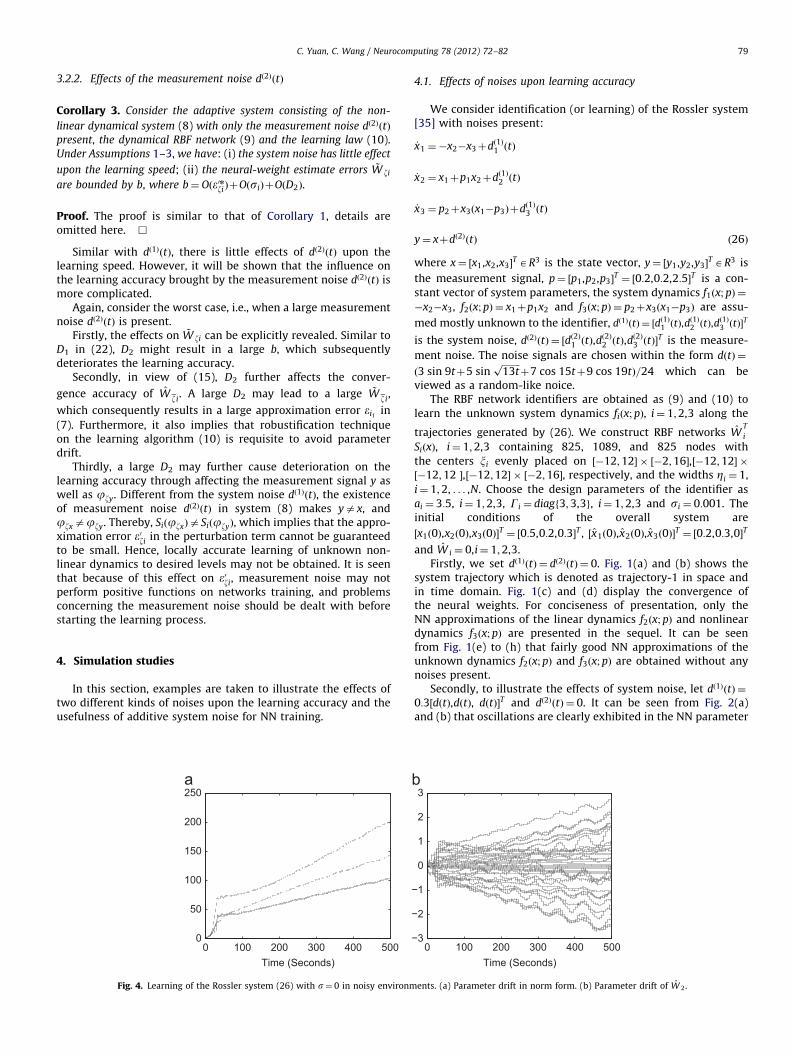
Fig. 4. Learning of the Rossler system (26) with s¼ 0 in noisy environm
4.1. Effects of noises upon learning accuracy
We consider identification (or learning) of the Rossler system[35] with noises present:
_x1 ¼�x2�x3þdð1Þ1 ðtÞ
_x2 ¼ x1þp1x2þdð1Þ2 ðtÞ
_x3 ¼ p2þx3ðx1�p3Þþdð1Þ3 ðtÞ
y¼ xþdð2ÞðtÞ ð26Þ
where x¼ ½x1,x2,x3�T AR3 is the state vector, y¼ ½y1,y2,y3�
T AR3 is
the measurement signal, p¼ ½p1,p2,p3�T ¼ ½0:2,0:2,2:5�T is a con-
stant vector of system parameters, the system dynamics f1ðx; pÞ ¼
�x2�x3, f2ðx;pÞ ¼ x1þp1x2 and f3ðx;pÞ ¼ p2þx3ðx1�p3Þ are assu-
med mostly unknown to the identifier, dð1ÞðtÞ ¼ ½dð1Þ1 ðtÞ,dð1Þ2 ðtÞ,d
ð1Þ3 ðtÞ�
T
is the system noise, dð2ÞðtÞ ¼ ½dð2Þ1 ðtÞ,dð2Þ2 ðtÞ,d
ð2Þ3 ðtÞ�
T is the measure-
ment noise. The noise signals are chosen within the form dðtÞ ¼
ð3 sin 9tþ5 sinffiffiffiffiffiffiffiffi13tp
þ7 cos 15tþ9 cos 19tÞ=24 which can beviewed as a random-like noice.
The RBF network identifiers are obtained as (9) and (10) to
learn the unknown system dynamics fiðx; pÞ, i¼ 1;2,3 along the
trajectories generated by (26). We construct RBF networks WT
i
SiðxÞ, i¼ 1;2,3 containing 825, 1089, and 825 nodes with
the centers xi evenly placed on ½�12;12� � ½�2;16�,½�12;12� �½�12;12 �,½�12;12� � ½�2;16�, respectively, and the widths Zi ¼ 1,
i¼ 1;2, . . . ,N. Choose the design parameters of the identifier as
ai ¼ 3:5, i¼ 1;2,3, Gi ¼ diagf3;3,3g, i¼ 1;2,3 and si ¼ 0:001. Theinitial conditions of the overall system are
½x1ð0Þ,x2ð0Þ,x3ð0Þ�T ¼ ½0:5,0:2,0:3�T , ½x1ð0Þ,x2ð0Þ,x3ð0Þ�
T ¼ ½0:2,0:3,0�T
and W i ¼ 0,i¼ 1;2,3.Firstly, we set dð1ÞðtÞ ¼ dð2ÞðtÞ ¼ 0. Fig. 1(a) and (b) shows the
system trajectory which is denoted as trajectory-1 in space andin time domain. Fig. 1(c) and (d) display the convergence ofthe neural weights. For conciseness of presentation, only theNN approximations of the linear dynamics f2ðx; pÞ and nonlineardynamics f3ðx; pÞ are presented in the sequel. It can be seenfrom Fig. 1(e) to (h) that fairly good NN approximations of theunknown dynamics f2ðx; pÞ and f3ðx; pÞ are obtained without anynoises present.
Secondly, to illustrate the effects of system noise, let dð1ÞðtÞ ¼
0:3½dðtÞ,dðtÞ, dðtÞ�T and dð2ÞðtÞ ¼ 0. It can be seen from Fig. 2(a)and (b) that oscillations are clearly exhibited in the NN parameter
0 100 200 300 400 500−3
−2
−1
0
1
2
3
Time (Seconds)
ents. (a) Parameter drift in norm form. (b) Parameter drift of W 2.

C. Yuan, C. Wang / Neurocomputing 78 (2012) 72–8280
convergence, which leads to relatively poor approximation results off2ðx;pÞ and f3ðx; pÞ, as shown in Fig. 2(c)–(f). Accordingly, by lettingdð2ÞðtÞ ¼ 0:3½dðtÞ,dðtÞ,dðtÞ�T and dð1ÞðtÞ ¼ 0, we can observe fromFig. 3(a)–(f) that due to the existence of measurement noise,accurate learning may not be obtained as well as that in Fig. 1.
Thirdly, we examine the situation without using any robusti-fication technique on the learning algorithm (10), i.e., setting si ¼
0, and let dð2ÞðtÞ ¼ 0:5½dðtÞ,dðtÞ,dðtÞ�T , dð1ÞðtÞ ¼ 0. Apparently, para-meter drift immediately occurs, see Fig. 4(a) and (b).
−4 −2 0 2 4 6
−5
0
50
1
2
3
4
x1x2
x3
450 460 470 480 490 500−5
0
5
10
Time (Seconds)
Function approximation:f2:−;fn2:−−
0 100 200 300 400 500−10
−505
10
Time (Seconds)
Function approximation error2
−4 −2 0 2 4 6
−50
5−4
−2
0
2
4
6
x1
Approximation in space:f2:−;fne2:−−
x2
f2&
fne2
Fig. 5. Learning of the Rossler system (26) with additive system noise. (a) Trajectory-2
f2ðx; pÞ. (d) Function approximation of f3ðx; pÞ. (e) Approximation of f2ðx; pÞ along trajecto
space. (h) Approximation of f3ðx; pÞ in space.
4.2. Usefulness of system noise
It will be shown in this part that additive system noise can beused to improve the generalization ability of the RBF networks.
We further consider the Rossler system with noises (26).To illustrate the effectiveness of additive system noise, weset dð2ÞðtÞ � 0. According to Corollary 2 and the implementa-tion elements presented in Section 3.2.1, the system noise ischosen as dð1ÞðtÞ ¼ 0:3½dðtÞ,dðtÞ,dðtÞ�T , the RBF network identifier is
0 100 200 300 400 500−1
−0.5
0
0.5
1
1.5
Time (Seconds)
Partial parameter convergence:W2
450 460 470 480 490 500−10
−505
10
Time (Seconds)
Function approximation:f3:−;fn3:−−
0 100 200 300 400 500−10
−505
10
Time (Seconds)
Function approximation error3
−5051001234
−6
−4
−2
0
2
4
6
x3
Approximation in space:f3:−;fne3:−−
x1
f3&
fne3
in phase space. (b) Parameter convergence of W 2. (c) Function approximation of
ry-2. (f) Approximation of f3ðx; pÞ along trajectory-2. (g) Approximation of f2ðx; pÞ in

−10 −5 0 5 10−10−5
05
10−6
−4
−2
0
2
4
6
X1
X2
−10 −5 0 5 10−2
02
46
810−6
−4
−2
0
2
4
6
X1
X3
Fig. 5. (continued)
C. Yuan, C. Wang / Neurocomputing 78 (2012) 72–82 81
designed as
_x i ¼�aiðxi�yiÞþWT
i SiðyÞþdð1Þi ðtÞ, i¼ 1;2,3 ð27Þ
with the learning law (10). Note that all the other parameters ofthe system and identifier, including the distribution of theneurons, remain the same as those in Section 4.1.
As seen in Fig. 5(a), the system trajectory which is denoted astrajectory-2 explores larger areas in space when compared with thetrajectory-1 as shown by Fig. 1(a), which results in that more neuronsare involved and activated. This can be shown by Figs. 1(d) and 5(b).It is examined that distributed along the system trajectory-2, 194
neurons w.r.t WT
1S1ðyÞ, 296 neurons w.r.t WT
2S2ðyÞ and 202 neurons
w.r.t WT
3S3ðyÞ are activated, which is larger than that along the
trajectory-1 where about 171, 276 and 174 neurons are acti-vated correspondingly. As a result, in addition to the locally accuratelearning is achieved along trajectory-2, see Fig. 5(c)–(f), it can beobserved that better generalization capability of the RBF networks isobtained with good approximation over a larger region of the spacein Fig. 5(g) and (h) when compared with Fig. 1(i) and (j). It is verifiedthat with deterministic learning scheme, the generalization capabilityof RBF networks can be enhanced with satisfactory learning accuracyby employing additive system noise.
5. Conclusions
In this paper, performance of deterministic learning in noisyenvironments has been investigated. In particular, effects of twodifferent kinds of noises, i.e., system noise and measurementnoise, upon the learning performance are revealed. Based on theexplicit convergence bounds of a class of perturbed LTV systems, ithas been analyzed that while there is little effect upon the learningspeed, the noises has much influence on the learning accuracy.Compared with system noise, the effects of measurement noiseappear to be more complicated. Under the noisy environments,robustification technique on the learning algorithm is required toavoid parameter drift. Furthermore, it is shown that proper systemnoise may enhance the generalization ability of the RBF networks.
Future research of this topic lies in the following directions. Oneresearch direction is to extend the explicit results with respect tothe perturbed LTV system to more general forms, such as learningfrom NN control [10]. The second research direction would be toinvestigate the performance of recognition system of deterministiclearning theory in noisy environments. Another direction is toobtain the counterparts of these results in discrete-time cases, suchas deterministic learning of discrete-time systems and sampled-data systems.
Acknowledgment
The authors would like to thank the anonymous reviewers forthe constructive comments.
References
[1] K.S. Fu, Learning Control Systems, Plenum Press, NY, 1969.[2] K.S. Fu, Learning control systems: review and outlook, IEEE Trans. Autom.
Control 15 (1970) 210–221.[3] Y.Z. Tsypkin, Adaptation and Learning in Automatic Systems, Academic Press,
NY, 1971.[4] E.B. Kosmatopoulos, M.A. Christodoulou, P.A. Ioannou, Dynamical neural
networks that ensure exponential identification error convergence, NeuralNetworks 10 (1997) 299–314.
[5] S. Lu, T. Basar, Robust nonlinear system identification using neural-networkmodels, IEEE Trans. Neural Networks 9 (3) (1998) 407–429.
[6] R.M. Sanner, J.E. Slotine, Gaussian networks for direct adaptive control,IEEE Trans. Neural Networks 3 (1992) 837–863.
[7] K.S. Narendra, A.M. Annaswamy, Stable Adaptive Systems, Prentice-Hall, NJ,1989.
[8] S. Sastry, M. Bodson, Adaptive Control: Stability, Convergence, and Robust-ness, Prentice-Hall, Englewood Cliffs, NJ, 1989.
[9] C. Wang, D.J. Hill, Learning form neural control, IEEE Trans. Neural Networks17 (1) (2006) 130–146.
[10] T. Liu, C. Wang, D.J. Hill, Learning from neural control of nonlinear systems innormal form, Syst. Control Lett. 58 (2009) 633–638.
[11] C. Wang, D.J. Hill, Deterministic Learning Theory for Identification, Recogni-tion and Control, CRC Press, Boca Raton, FL, 2009.
[12] C. Wang, D.J. Hill, Deterministic learning and rapid dynamical patternrecognition, IEEE Trans. Neural Networks 18 (2007) 617–630.
[13] Z. Xue, C. Wang, T. Liu, Deterministic learning and robot manipulator control,in: Proceedings of the IEEE on International Conference on Robotics andBiomimetics, Sanya, China, 2007.
[14] C. Wang, T. Chen, Rapid detection of oscillation faults via deterministiclearning, in: Proceedings of 8th IEEE International Congress on Control andAutomation, Xiamen, China, 2010.
[15] A.S. Morse, Global stability of parameter-adaptive control systems,IEEE Trans. Autom. Control AC-25 (3) (1980).
[16] K.J. Astrom, Bohn, Numerical identification of linear dynamic systems fromnormal operating records, in: P.H. Hammond (Ed.), Proceedings of the 2ndIFAC Symposium on Theory Self-Adaptive Control Systems, National PhysicalLaboratory, Teddington, UK, 1965, pp. 96–111.
[17] B.O. Anderson, Exponential stability of linear equations arising in adaptiveidentification, IEEE Trans. Autom. Control AC-22 (1977) 83–88.
[18] E. Panteley, A. Loria, A. Teel, Relaxed persistency of excitation for uniformasymptotic stability, IEEE Trans. Autom. Control 46 (12) (2001).
[19] A.P. Morgan, K.S. Narendra, On the stability of nonautonomous differentialequations _x ¼ ½aþbðtÞ�x, with skew symmetric matrix b(t), SIAM J. ControlOptim. 15 (1) (1977).
[20] A.P. Morgan, K.S. Narendra, On the uniform asymptotic stability of certainlinear nonautonomous differential equations, SIAM J. Control Optim. 15 (1)(1977).
[21] P.A. Ioannou, J. Sun, Robust Adaptive Control, Prentice-Hall, Englewood Cliffs,NJ, 1995.
[22] R. Ortega, On Morse’s new adaptive controller: parameter convergence andtransient performance, IEEE Trans. Autom. Control 38 (8) (1993).
[23] J.S. Lin, I. Kanellakopoulos, Nonlinearities enhance parameter convergence inoutput-feedback systems, IEEE Trans. Autom. Control 43 (2) (1998).

C. Yuan, C. Wang / Neurocomputing 78 (2012) 72–8282
[24] J. Park, I.W. Sandberg, Universal approximation using radial-basis-functionnetworks, Neural Comput. 3 (2) (1991) 246–257.
[25] J.T. Lo, Finite-dimensional sensor orbits and optimal nonlinear filtering,IEEE Trans. Inf. Theory IT-18 (5) (1972) 583–588.
[26] D. Gorinevsky, On the persistency of excitation in radial basis functionnetwork identification of nonlinear systems, IEEE Trans. Neural Networks6 (5) (1995).
[27] A.J. Kurdila, F.J. Narcowich, J.D. Ward, Persistency of excitation in identifica-tion using radial basis function approximations, SIAM J. Control Optim. 33 (2)(1995) 625–642.
[28] L.P. Shilnikov, Methods of Qualitative Theory in Nonlinear Dynamics, Part II,World Scientific, Singapore, 2001.
[29] C. Yuan, C. Wang, Persistency of excitation and performance of deterministiclearning, Syst. Control Lett., doi:10.1016/j.sysconle.2011.08.002, in press.
[30] L. Holmstrom, P. Koistinen, Using additive noise in back-propagation train-ing, IEEE Trans. Neural Networks 3 (1992) 24–38.
[31] C. Wang, G. Chen, S.S. Ge, Smart neural control of uncertain nonlinearsystems, Int. J. Adaptive Control Signal Process. 17 (2003) 467–488.
[32] S. Haykin, Neural Networks: A Comprehensive Foundation, 2nd ed., Prentice-Hall, Englewood Cliffs, NJ, 1999.
[33] J.T. Spooner, K.M. Passino, Stable adaptive control using fuzzy systems andneural networks, IEEE Trans. Fuzzy Syst. 4 (1996) 339–359.
[34] M. Krstic, I. Kanellakopoulos, P. Kokotovic, Nonlinear and Adaptive ControlDesign, John Wiley, NY, 1995.
[35] O.E. Rossler, An equation for continuous chaos, Phys. Lett. A 57 (1976)397–398.
Chengzhi Yuan the Master candidate at the Center forControl and Optimization, School of Automation, SouthChina University of Technology. His research interestcovers adaptive NN control/identification, determinis-tic learning theory.
Cong Wang received the B.E. and M.E. degrees fromthe Beijing University of Aeronautic and Astronautics,Beijing, China, in 1989 and 1997, respectively, and thePh.D. degree from the National University of Singa-pore, Singapore, in 2002. He carried out post-doctoralresearch at the City University of Hong Kong, Kowloon,Hong Kong, from 2001 to 2004. Currently, he is aProfessor at the School of Automation, South ChinaUniversity of Technology, Guangzhou, China. He hasauthored and co-authored over 60 papers in interna-tional journals and conferences, and is a co-author ofthe book Deterministic Learning Theory for Identifica-
tion, Recognition and Control (Boca Raton, FL: CRCPress, 2009). His current research interests include deterministic learning theory,dynamical pattern recognition, pattern-based intelligent control, and oscillationfault diagnosis.