processes

Article

Parallel Implementation of the Deterministic Ensemble KalmanFilter for Reservoir History Matching

Lihua Shen * , Hui Liu and Zhangxin Chen

�����������������

Citation: Shen, L.; Liu, H.; Chen Z.

Parallel Implementation of the

Deterministic Ensemble Kalman

Filter for Reservoir History Matching.

Processes 2021, 9, 1980. https://

doi.org/10.3390/pr9111980

Academic Editor: Simant Upreti and

Jean-Pierre Corriou

Received: 11 September 2021

Accepted: 3 November 2021

Published: 6 November 2021

Publisher’s Note: MDPI stays neutral

with regard to jurisdictional claims in

published maps and institutional affil-

iations.

Copyright: © 2021 by the authors.

Licensee MDPI, Basel, Switzerland.

This article is an open access article

distributed under the terms and

conditions of the Creative Commons

Attribution (CC BY) license (https://

creativecommons.org/licenses/by/

4.0/).

Department of Chemical and Petroleum Engineering, University of Calgary, 2500 University Dr NW,Calgary, AB T2N 1N4, Canada; Hui.Liu@cmgl.ca (H.L.); zhachen@ucalgary.ca (Z.C.)* Correspondence: lihua.shen@ucalgary.ca; Tel.: +1-403-210-6526

Abstract: In this paper, the deterministic ensemble Kalman filter is implemented with a paralleltechnique of the message passing interface based on our in-house black oil simulator. The imple-mentation is separated into two cases: (1) the ensemble size is greater than the processor numberand (2) the ensemble size is smaller than or equal to the processor number. Numerical experimentsfor estimations of three-phase relative permeabilities represented by power-law models with bothknown endpoints and unknown endpoints are presented. It is shown that with known endpoints,good estimations can be obtained. With unknown endpoints, good estimations can still be obtainedusing more observations and a larger ensemble size. Computational time is reported to show that therun time is greatly reduced with more CPU cores. The MPI speedup is over 70% for a small ensemblesize and 77% for a large ensemble size with up to 640 CPU cores.

Keywords: history matching; DEnKF; relative permeability; power-law model; parallel computing

1. Introduction

The ensemble Kalman filter (EnKF) is a data assimilation method to estimate poorlyknown model solutions and/or parameters by integrating the given observation data. Itwas introduced by Evensen [1] and has attracted a lot of attention in the fields of weatherforecasting sciences, oceanographic sciences and reservoir engineering. Regarded as aMonte Carlo formulation of the Kalman Filter, it is applied to each ensemble forecast inan analysis step. The deterministic ensemble Kalman filter (DEnKF) is a variation of theEnKF which has an asymptotic match of the analysis error covariance from the Kalmanfilter theory with a small correction and without any perturbed observation; its form issimpler while its robust property is still kept [2].

The EnKF has been introduced to reservoir engineering in the past decade. As a dataassimilation method for history matching, the EnKF can be used to assimilate differentkinds of production data, estimate model parameters and adjust dynamical variables. Itwas first applied to history matching by Nævdal [3,4]. A detailed review was given byAanonsen et al. [5]. It has been used to estimate reservoir porosity and permeabilitysuccessfully [4,6,7]. It has also been adopted to estimate relative permeability and capillarypressure curves with good accuracy [8–11]. Nevertheless, for most of the applications,hundreds of the ensemble members are required to guarantee the accuracy of an estimation.For example, an estimation of endpoints of relative permeability curves is challenging; agood estimation can only be obtained in limited cases [8,9] and requires a large ensemblesize. Therefore, a serial run of simulations is very time-consuming. Furthermore, forlarge-scale numerical models, the memory of one single processor may even not be enoughfor a simulation with one ensemble member. Therefore, the parallel technique becomes anatural choice to reduce the computational time and make large-scale models feasible.

The parallel technique has been successfully applied in many fields including atmo-sphere and oceanographic sciences. A multivariate ensemble Kalman filter was imple-mented on a massively parallel computer architecture for the Poseidon ocean circulation

Processes 2021, 9, 1980. https://doi.org/10.3390/pr9111980 https://www.mdpi.com/journal/processes

Processes 2021, 9, 1980 2 of 20

model [12]. At an EnKF forecast step, each ensemble member is distributed to a differentprocessor. To parallelize an analysis step, the ensemble is transposed over processorsaccording to domain decomposition. A parallelized localization implementation was re-ported in [13] based on domain decomposition. As for the reservoir history matching,the parallel technique has not been well developed. An automatic history matching mod-ule with distributed and parallel computing was done by Liang et al. using weigthedEnKF [14], where two-level high-performance computing is implemented, distributingensemble members simultaneously by submitting all the simulation jobs at the same timeand simulating each ensemble member in parallel. A parallel framework was given byTavakoli et al. [15] using the EnkF and ensemble smoother (ES) methods based on thesimulator IPARS, in which a forecast step was parallelized while an analysis step wascomputed by one central processor. It discussed the case where the processor number isfewer than the ensemble size and each processor is in charge of one or several ensemblemembers according to its simulation speed. In their another work [16], the case where theprocessor number is greater than the ensemble size was also discussed. For parallelizingan analysis step, the parallelization was carried out by partitioning a matrix in a row-wisemanner. Comparing to the EnKF, ES requires less time to assimilating the data as it doesnot need to synchronize all the ensemble members at the analysis step. However, for thelarge data point problems, the matrices become very large, resulting in long computationaltime and large memory requirements for the inversion.

Although the implementation of the parallel technique was explored in the abovepapers, good computational efficiency has not been obtained, even with high performancesimulators. One important reason is that after each analysis step, updated variable valueswere written on a disk and read by different processors to restart a simulator. A largenumber of inputs/outputs not only waste the disk space, but also slow down accessing,reading and writing. On the other hand, an analysis step must have been done afterall the simulations in a forecast step are finished. This synchronization determines thatat every forecast step, the simulation time equals the maximum run time among all theprocessors. From the parallel aspect, MPI inputs/outputs have poor performance oncommon computer clusters. Load and storage operations are more time-consuming thanmultiplication operations. Moreover, parallelization of an analysis step needs messagepassing multiple times. According to the above published papers, the parallel efficiencywas generally lower than 50% with an ensemble of no more than 200 members comparedto the ideal efficiency 100%.

In contrast to the traditional EnKF method, some modifications of this method havebeen done and different filters have been developed, such as Ensemble Square Root Filters(ESRFs) [17,18] and deterministic Ensemble Kalman filters (DEnKF) [2] that give betterperformance in certain conditions. First proposed by Sakov et al. [17], DEnKF can beregarded as a linear approximation to the ESRF under a small analysis correction condition,and it combines the simplicity of the ESRF and the versatility of the traditional EnKF. Itsrobust property has been shown by numerical experiments [17]. Despite the intensiveresearch and implementation of EnKF, to our knowledge, the DEnKF has not been adoptedin the reservoir history matching field yet.

In this paper, the DEnKF is implemented for reservoir history matching with a paralleltechnique and our in-house parallel black oil simulator. Both forecast and analysis stepsare parallelized according to a relationship between an ensemble size and a processornumber. To improve the computational efficiency, several switches are defined to controlthe input/output and set by the user. The restart of the simulator is slightly modified tocoordinate the history matching implementation. The simulator is called as a function fromour platform library.

This paper is organized as follows. First, our black oil simulator is briefly introduced.After that, the EnKF and DEnKF are given, followed by a parallel technique used in ourcomputations. Based on this technique, numerical experiments on the estimation of relativepermeability curves with known endpoints and unknown endpoints are presented. The

Processes 2021, 9, 1980 3 of 20

parallel speedup is reported to show the computational efficiency. Conclusions are givenat the end of this paper.

2. Black Oil Simulator

In this paper, a black oil model is simulated. Using the mass conservation law andDarcy’s law on water, oil and gas, the following equations can be obtained [19,20]:

∇(KKrwρwµw∇Φw) + qw = ∂(φρwSw)

∂t

∇(KKroρoo

µo∇Φo) + qo =

∂(φρooSo)

∂t

∇(KKroρgo

µo∇Φo) +∇(

KKrgρgg

µg∇Φg) + qg

= ∂(φρgo So)

∂t +∂(φρ

ggSg)

∂t .

(1)

In these equations, K is the absolute permeability tensor of a reservoir; Krl and Sl arethe relative permeability and saturation of phase l (l = w, o, g), respectively; ρw is the waterdensity; ρo

o is the oil component density in the oil phase; ρgo is the gas component density in

the oil phase; and ρgg is the gas component density in the gas phase. The potential of phase

l has the formΦl = Pl − Gρlz

where Pl is the pressure of phase l (l = w, o, g), G is the magnitude of the gravitationalconstant and z is the depth of the position. The saturations of water, oil and gas satisfy

Sw + So + Sg = 1. (2)

For the pressures of the water, oil and gas, we have

pcow(Sw) = Po − Pw

pcog(Sg) = Pg − Po

where Pcow is the capillary pressure between oil and water and Pcog is the capillary pressurebetween oil and gas. We choose P = Po, Sw and Sg as the primary unknowns, and they canbe obtained from Equations (1). There are production and injection wells in a reservoir.The rates of these wells have the forms

qw = WI ∗ KKrwµ ρw[PBH − P− GρBH(zBH − z)]

qoo = WI ∗ KKro

µ ρoo[PBH − P− GρBH(zBH − z)]

qgo = WI ∗ KKrg

µ ρgo [PBH − P− GρBH(zBH − z)]

qgg = WI ∗ KKrg

µ ρgg[PBH − P− GρBH(zBH − z)].

(3)

Here, qg = qgo + qg

g, qo = qoo and WI is the well index which is known [19,20].

In summary, four unknowns P, Sw, Sg and PBH are to be solved fromEquations (1)–(3). An in-house parallel simulator is used to simulate the black oil model.Developed on our platform PRSI, it uses the finite (volume) difference method with up-winding schemes [20,21]. Its highly computational efficiency and good parallel scalabilityhave been shown by numerical experiments that simulate very large scale models withmillions of grid cells using thousands of CPU cores [22]. In our implementation, thissimulator is called as a function from the library.

3. EnKF and DEnKF

EnKF is an efficient data assimilation method which has been used in history matchingof reservoir simulation to estimate model parameters with uncertainty such as porosity

Processes 2021, 9, 1980 4 of 20

and permeability. It is a Monte Carlo method in which an ensemble of reservoir models isgenerated according to the given statistic properties. The ensemble can be written as

Yk = [yk,1, yk,2, · · · , yk,Ne ], k = 1, · · · , Nt,

where subscript k is the time index, Ne is the ensemble size and Nt is the total numberof the assimilation steps. Each yk,j denotes one sample vector. For the history matchingof reservoir simulation, yk,j is named a state vector which consists of two parts: modelvariables m and observation data d. The model variables include static variables mst (suchas porosity, absolute permeability and relative permeability parameters) and dynamicalvariables mdyn (such as pressure and saturation). The observation data includes wellmeasurement data such as production rates, injection rates and bottom hole pressures.Thus, a state vector can be written as

yk,j =

[md

]k,j

=

mstmdyn

d

k,j

.

We denote the length of the vectors mk,j and dk,j by Nm,k and Nd,k, and define thematrix Hk as Hk = [0 I], where 0 is the Nd,k × Nm,k zero matrix and I is the Nd,k × Nd,kidentity matrix. Then, it is obvious that

dk,j = Hkyk,j.

Note that the observation vector dk,j is random and can be expressed as

dk,j = dtruek + εk,j, k = 1, · · · , Nt, j = 1, · · · , Ne (4)

where dtruek is the true value of the observation and εk,j is a vector of the error at the kth

time step. According to Burgers et al. [23], vector εk,j consists of measurement errors andnoise. Both of them are assumed Gaussian and uncorrelated. Thus, the covariance of εk,jcan be simplified to a diagonal matrix CD,k.

At the time step tk when observation data is available, a reservoir simulator stops tostart the data assimilation. The traditional form of an EnKF analysis step is as follows [1]:

yak,j = y f

k,j + Kk(dk,j − Hky fk,j), (5)

Kk = C fy,k HT

k (HkC fy,k HT

k + CD,k)−1 (6)

where the superscript f means a forecast solution that is computed from the simulator, thesuperscript a means an analysis ensemble updated by data assimilation, and T denotes thetranspose of a vector or a matrix. Kk named the Kalman gain can be regarded as a weightedmatrix that controls which sample has more influence on updating. In Equation (6), C f

y,k is

the covariance matrix of the state vector y fk,j from simulation, i.e.,

C fy,k = cov(Y f

k , Y fk ) =

1Ne − 1

(Y fk − Y f

k )(Yf

k − Y fk )

T

where Y fk is a matrix in which every column vector is the mean value of the ensemble

members. Denoting the mean of all the ensemble members Y fk as y f

k , then Y fk can be written

as Y fk = y f

k 1T with 1 a vector of ones.Note that for the convenience of numerical implementation, Equations (5) and (6) can

be expresses asYa

k = Y fk X5,k (7)

Processes 2021, 9, 1980 5 of 20

where the Ne × Ne matrix X5,k is calculated from Y fk . The form of X5,k is given by

Evensen [1,24].Here, we drop the subscript k of the above notations for simplicity. For the DEnKF,

denoting A f = Y f − Y f and Aa = Ya − Ya as the ensemble anomalies of the forecastensemble Y f and the analysis ensemble Ya, respectively, then they have the relationship [17]

Aa = A f − 12

KHA f .

Denote TR = I− 12(Ne−1) A f T HT(HP f HT + CD)

−1HA f and write it in the ensembleform

Ya = Y f X5.

Then, X5 has the form [17,24]

X5 = [1

Ne11T + w1T + (I− 1

Ne11T)TR],

and w is a vector which satisfies ya = y f + A f w and has the form

w =1

Ne − 1A f T

HT(HC fy HT + CD)

−1(d− Hy f ).

Therefore, to obtain the analysis ensemble Ya, X5 and its multiplication with theforecast ensemble Y f need to be calculated. This is similar to the traditional EnKF andthe ESRF, while TR has a simpler form for the DEnKF. It will be seen in our numericalexperiments that the performance is quite good.

4. Parallel Technique

In most cases, EnKF requires an ensemble of hundred data points to assimilate his-tory data. Between every two assimilation steps, a reservoir model is simulated with asmany times as the ensemble size, which is extremely computational costly. In this work,the MPI parallel technique is adopted to improve the computing efficiency and reducethe computing time. Note that from the beginning of the EnKF process, many ensemblemembers of parameters are generated based on statistical properties and then for eachensemble member, reservoir simulation is conducted independently. Based on this consid-eration, the ensemble members can be distributed to all the processors in balance. Eachprocessor is in charge of an equal number of ensemble members and simulating at thesame time. When it comes to a data assimilation step where a processor cannot computeindependently, analysis values are calculated by communicating with each other using theMPI technique. After all data is assimilated, it comes to the prediction step. In this step,each processor independently simulates the reservoir model with the distributed ensemblemembers which have already been adjusted. From this procedure, it can be seen that theMPI technique can be adopted in the EnKF method naturally.

There are the following steps for the programming implementation:

1. get the ensemble:

(a) if step =0,

i. if readrdm = TRUE, read static variables only;ii. else generate ensemble of the static variables.

(b) else

i. if readens = TRUE, read both static variables and dynamic variablevalues from files;

ii. else get the static variable values and dynamic variable values fromthe memory.

Processes 2021, 9, 1980 6 of 20

2. use the ensemble to simulate the reservoir and get Y f ; if predict = TRUE, go to 7.3. if readens = TRUE, write both static dynamic variable values and dynamic variable

values to the files.4. read observations from the files.5. assimilate data using DEnKF and get Ya.6. if readens = TRUE, write both static dynamic variable values and dynamic variable

values to the files; go to 1.7. end

The flow chart of the implementation is given in Figure 1. In our implementation, forthe result visualization purpose, two switches writeens and writepars can also be set by theuser. When writeens = TRUE, all the dynamic and static variables are written to the filesbut not necessarily read during running. When writepars = TRUE, only static variables arewritten. The ensembles of the dynamic and static variables are always output to files at thelast analysis step.

read in ensembles?

Yes

read ensemble files

generate ensemble

of paramters

write ensemble?

No

reservoir simulation

write ensemble to files get values of observations d

and dynamic variables m_dyn

write observations and/or

dynamic variables?write values to files

Yes

No

data assimilation using

DEnKF to get Y^a

step = step + 1

write analysis values

of m_st, m_dyn or d?write analysis values

Yes

No

start

No

step =0?

Yes

No

No

predict?No

end

Yes

Yes

predict

Figure 1. The flowchart of the algorithm.

Processes 2021, 9, 1980 7 of 20

For the switch readens, if it is set to TRUE by the user, all the dynamic variables and thestatic variables are written to the files on a hard disk and the corresponding variable spacesallocated in the computer are freed after they are written at the each data assimilation step.After one cycle is done and before the next reservoir simulation starts, these data are readin from those files to restart the reservoir simulator. However, when the ensemble sizeis large, the performance of IO (Input and Output) is poor. Many small files written tothe hard disk can not only waste space of the hard disk, but also are slow to access. Theefficiency becomes even lower when the dynamic variable values are written to the filesusing MPI/IO. Nevertheless, MPI/IO must be used in a certain condition. For example,when the ensemble size is smaller than the processor size, for each ensemble, the reservoirsimulation is done by several processors in parallel. Therefore, after the simulation, thevector of each dynamic variable is partially distributed in several processors. It is inevitableto write a dynamic vector to one file in the grid cell order using MPI/IO. To avoid readingand writing data to files, our simulator is slightly modified and the switch readens can beset to FALSE by the user so that both the dynamic variables and the static variables arealways in the memory during computing and their values are updated every step. Onemight worry about that these variables would occupy too much computer memory. In fact,the ensemble members are equally distributed in the processors from the beginning. Theallocation of the ensemble members and the simulations in different processes are shownin Figure 2. In this figure, the solid box denotes one simulation, the dash dot box denotesone processor and the dot box denotes the processor group. If the ensemble size Ne islarger than the processor number p, each processor only has Ne

p ensemble numbers. If theensemble size is smaller than the processor number, each simulation with one ensemblemember is carried out by p

Ne processors. The vector of each dynamic variable value isequally distributed to these p

Ne processors. Therefore, when multiple computer nodes andCPU cores are used on a supercomputer, each core only spends limited memory to savethe dynamic variable vectors. It is not costly to keep these variables all the time.

S1

P1 P2 P

one processorone simulation

p

Ne/p

1 +Ne/p

2 *Ne/p

1 +(p-1)Ne/p

2 +(p-1) Ne/p

Ne

S2

S

S

2 +Ne/pS

S

S

S

S

Sj : jth ensemble member Pj : processor j

(a)

G

P1

P2

Pp/Ne

G G

P1+p/Ne

P2+p/Ne

P2*p/Ne

P1+ (Ne-1)p/Ne

f

1

f

2

f

Ne

Ga

1

Ga

2

Ga

Ne

one processorone simulation one processor group

S1 S2 SNe

P2+ (Ne-1)p/Ne

Pp

Sj : jth ensemble member Pj : processor j

(b)

Figure 2. The allocation of the ensemble members and the simulations in different processors: (a)Ne > p and (b) Ne <= p.

As an ensemble size is generally much smaller than the length of a state vector, themain computational cost of an analysis step is the matrix multiplication in Equation (7)which is computed in parallel after the matrix X5 is computed sequentially by one processor.Supposing that the division of Ne and p is an integer, there are two different cases:

• Ne > p. If the ensemble size Ne is larger than the processor number p, each processorruns the simulation for Ne

p times in every cycle independently and get the dynamicvariable values corresponding to its ensemble members (see Figure 2a). Therefore,

Processes 2021, 9, 1980 8 of 20

each processor obtains one or several complete columns of matrix Y f . For processorj (j = 1, · · · , p), by multiplying these columns by X5, it gets a matrix Ya,j with a sizethe same as that of matrix Y f . Note that Ya = ∑

pj=1 Ya,j so the analysis results can be

obtained by adding all the Ya,j from every processor using the function MPI_Allreduce.The matrix multiplication is illustrated by Figure 3.

• Ne <= p. If the ensemble size Ne is smaller than or equal to the processor num-

ber p, each simulation is done by the processor group G fj = {P1+j∗p/Ne , P2+j∗p/Ne ,

· · · , Pp/Ne+j∗p/Ne }, (j = 0, · · · , Ne − 1) (see Figure 2b) with pNe

processors included(note that they are at the same time in one simulation box). The computing tasksof the processors in this group are assigned by the simulator based on the domaindecomposition. According to the load balancing principle, the vector entries of eachdynamic variable are equally distributed and the variable values are not completein each processor. For the processor group Ga

j = {Pj, Pj+p/Ne , · · · , Pj+(Ne−1)∗p/Ne}(j = 1, · · · , p/Ne) (see Figure 2b) by multiplying these vector entries of its own withX5, the processors in Group Ga

j get the matrices Ya,j, Ya,j+p/Ne ,· · · Ya,j+(Ne−1)∗p/Ne ,respectively. By gathering these values in its own group Ga

j , every processor in this

group gets the value ∑Ne−1i=0 Ya,j+i∗(p/Ne) which includes the corresponding updated

vector entries. The distribution of the matrix entries is displayed in Figure 4. Theprocessor groups are created by the function lMPI_Comm_split.

P1 P j P

*

=

p

j = 1

X_5

P

P j

* X_500

Figure 3. The matrix multiplication of Y f and X5 in case Ne > p. Pi (i=1, · · · , p) denotes the ithprocessor.

in Group Ga

j

P1

Pj

Pp/Ne

Pj + i*p/Ne

Pj + (Ne-1)*p/Ne

P1

Pj

Pp/Ne

Pj + i*p/Ne

Pj + (Ne-1)*p/Ne

Y = f

One variable

One variable

S1 Si SNe

Figure 4. The entries of the matrix Y f on different processors in case Ne <= p. Si (i = 1, · · · , Ne)denotes the ith ensemble member. Pi (i=1, · · · , p) denotes the ith processor.

Processes 2021, 9, 1980 9 of 20

When Ne > p and the division of Ne and p is not an integer, some of the processorsget fewer ensemble members than the others and thus simulate a reservoir with less time.However, the algorithm is still the same. When Ne <= p and the division of p and Ne is notan integer, special treatment and more message passing are required when gathering thevectors since for some of the ensemble members the corresponding reservoir simulationsare conducted by fewer processors than the others.

For a large-scale reservoir model that requires a large number of grid cells for dis-cretization, the simulation with every ensemble member is time-consuming. In this case,the ensemble is not distributed to processors. Instead, the models with different ensemblemembers are simulated sequentially. Each model with one ensemble member is simulatedby all the processors in parallel. Although the simulation run is very costly, it is obviouslya trivial case of our discussion from the programming design aspect.

5. Numerical Experiments

In this section, the history matching of the SPE-9 benchmark model is presented.Estimations of relative permeability curves with known endpoints and unknown endpointsare plotted. With each estimation, the corresponding prediction results are obtained.Following that, the parallel efficiency of computations is reported.

5.1. SPE-9 Black Oil Model

SPE-9 is a three-phase black oil model with 24× 25× 15 grid blocks. The grid sizes inthe x- and y-direction are both 300 ft. The z-direction grid size is 20, 15, 26, 15, 16, 14, 8, 8, 18,12, 19, 18, 20, 50, and 100 ft from top to bottom. It has heterogeneous absolute permeability.The porosity varies layer-by-layer in the z-direction and equals 0.087, 0.097, 0.111, 0.16,0.13, 0.17, 0.17, 0.08, 0.14, 0.13, 0.12, 0.105, 0.12, 0.116 and 0.157 from top to bottom. Thedensities of water, oil and gas are 63.021, 44.986, and 0.0701955 lbm/ft3, respectively, witha reference pressure of 3600 psi. The bubble pressure is 3600 psi at the reference depth9035 ft. The rock compressibility and water compressibility are both 1.0× 10−6 (1/psi).The total production days are 900 days.

There are 26 wells in the reservoir: one injector and 25 producers. The injector’sperforation is at layer 11 to layer 15 while each producer’s perforation is at layers 2, 3and 4. The injector has a maximum standard water rate of 5000 bbl/day and a maximumbottom hole pressure of 4543.39 psi. The radius of each well is 0.5 ft. The schedule can beobtained from the keyword file in the document folder of the commercial software such asCMG IMEX.

The oil relative permeability in three phases can be obtained from the water and oiltwo-phase relative permeabilities and the gas and oil two-phase relative permeabilities [25].To represent a relative permeability curve by a power-law function (e.g., based on anempirical Corey’s model [26]), a power-law model only requires to determine the endpointsand exponential factors. Power-law models of water and oil relative permeabilities can bewritten as

krw(Sw) = aw

(Sw − Swc

1− Swc − Sorw

)nw

= awSnwwD (8)

krow(Sw) = aow

(1− Sw − Sorw

1− Swc − Sorw

)now

= aow(1− SwD)now . (9)

whereSwD =

Sw − Swc

1− Swc − Sorw.

Processes 2021, 9, 1980 10 of 20

Similarly, power-law representations of gas and oil relative permeabilities are

krg(Sg) = ag

(Sg − Sgc

1− Sgc − Sorg − Swc

)ng

= agSnggD (10)

krog(Sg) = aog

(1− Sg − Sorg − Swc

1− Sgc − Sorg − Swc

)nog

= aog(1− SgD)nog . (11)

with

SgD =Sg − Sgc

1− Sorg − Sgc − Swc.

Equations (8)–(11) will be used in our computing.We consider the case where the oil relative permeability is defined by normalizing its

effective permeability by using its value at the critical water saturation, i.e.,

krow =kow(Sw)

kow(Swc)

where kow is the effective oil permeability. Then krow(Swc) = 1 holds, which leads to aow = 1.Similarly, for the gas and oil relative permeabilities, if the gas relative permeability isdefined by normalizing its effective permeability by using its value at the irreducible gassaturation, i.e.,

krog =kog(Sg)

kog(Sgc)

where kog is the oil effective permeability, then krog(Sgc) = 1 and thus aog = 1. Consequently,10 parameters are left to define the relative permeability curves. Written as a parametervector, they are

mst = [aw, nw, now, Swc, Sorw,

ag, ng, nog, Sgc, Sorg]. (12)

Note that the endpoints are fixed by 6 parameters: aw, Swc, Sorw, ag, Sgc and Sorg. Ifthese parameters are known, only 4 parameters are left and the endpoints of the relativepermeability curves are fixed. Thus, the parameter vector becomes

mst = [no, now, ng, nog]. (13)

For an estimation with known endpoints, the observations are the cumulative waterproduction rate (CWPR), cumulative oil production rate (COPR) and cumulative gasproduction rate (CGPR) of all the 25 production wells as well as the cumulative waterinjection rate (CWIR) of the injection well. For an estimation with unknown endpoints, theobservations are the oil production rates, the gas production rates, the water productionrates of the 25 producers, the water injection rate of the injector and the bottom-holepressures of all the wells. All the rates are obtained from our simulator PRSI. All the data isperturbed by a Gaussian distribution error with 5% variance.

5.2. Estimation with Known Endpoints

As mentioned before, when the endpoints are known, only four unknowns are leftas shown in Equation (13). In this work, totally 160 Gaussian realizations are generatedfor these parameters to assimilate the observations. The days on which the observationsare assimilated are listed in Table 1. The first step of data assimilation is on the 12th dayand the last one on the 552nd day. After that, each updated ensemble member with thepermeability parameter values at the last step is used to simulate the model until the end

Processes 2021, 9, 1980 11 of 20

day to predict the rates. The reference values, together with the means and the variancesof the unknowns used to generate the ensemble, are listed in Table 2. The adjusted meanvalues after data assimilation and their relative errors different from the reference valuesare also listed in this table.

Table 1. The days on which data is assimilated.

step 1 2 3 4 5 6 7 8day 12 32 50 67 87 102 122 141

step 9 10 11 12 13 14 15 16day 162 182 200 217 237 257 277 297

step 17 18 19 20 21 22 23 24day 312 332 352 367 387 407 422 442

step 25 26 27 28 29 30day 462 480 497 517 537 552

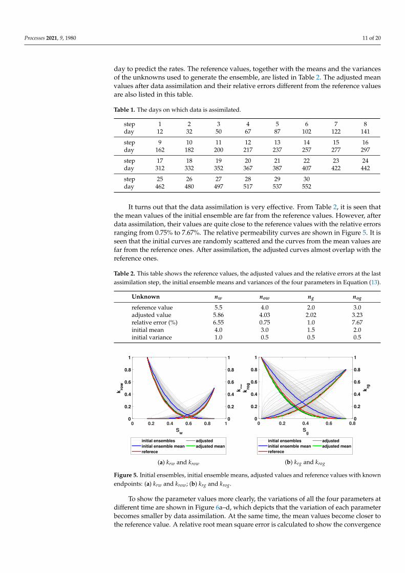
It turns out that the data assimilation is very effective. From Table 2, it is seen thatthe mean values of the initial ensemble are far from the reference values. However, afterdata assimilation, their values are quite close to the reference values with the relative errorsranging from 0.75% to 7.67%. The relative permeability curves are shown in Figure 5. It isseen that the initial curves are randomly scattered and the curves from the mean values arefar from the reference ones. After assimilation, the adjusted curves almost overlap with thereference ones.

Table 2. This table shows the reference values, the adjusted values and the relative errors at the lastassimilation step, the initial ensemble means and variances of the four parameters in Equation (13).

Unknown nw now ng nog

reference value 5.5 4.0 2.0 3.0adjusted value 5.86 4.03 2.02 3.23relative error (%) 6.55 0.75 1.0 7.67initial mean 4.0 3.0 1.5 2.0initial variance 1.0 0.5 0.5 0.5

0 0.2 0.4 0.6 0.8 1

Sw

0

0.2

0.4

0.6

0.8

1

kro

w

0

0.2

0.4

0.6

0.8

1

krw

initial ensembles

initial ensemble mean

referece

adjusted

adjusted mean

(a) krw and krow

0 0.2 0.4 0.6 0.8

Sg

0

0.2

0.4

0.6

0.8

1

kro

g

0

0.2

0.4

0.6

0.8

1

krg

initial ensembles

initial ensemble mean

referece

adjusted

adjusted mean

(b) krg and krog

Figure 5. Initial ensembles, initial ensemble means, adjusted values and reference values with knownendpoints: (a) krw and krow; (b) krg and krog.

To show the parameter values more clearly, the variations of all the four parameters atdifferent time are shown in Figure 6a–d, which depicts that the variation of each parameterbecomes smaller by data assimilation. At the same time, the mean values become closer tothe reference value. A relative root mean square error is calculated to show the convergence

Processes 2021, 9, 1980 12 of 20

of the parameters. It is a normalized difference between the mean value of the updatedparameter vector and its true value, i.e.,

REst =

√√√√ 1Nmst

Nmst

∑i=1

(mmean

st,i −mtruest,i

mtruest,i

)2

× 100% (14)

where mst,i is the ith component of the vector mst and Nmst is the length of the vector [9].Figure 6e depicts the relative root mean square error of the relative permeability modelvector. It shows that at the last assimilation step, the relative root mean square error dropsto 5%.

0 100 200 300 400 500

Time (day)

0

2

4

6

8

nw

adjusted nw

reference nw

(a) nw

0 100 200 300 400 500

Time (day)

2

3

4

5

no

w

adjusted now

reference now

(b) now

0 100 200 300 400 500

Time (day)

0

1

2

3

ng

adjusted ng

reference ng

(c) ng

0 100 200 300 400 500

Time (day)

1

2

3

4

no

g

adjusted nog

reference nog

(d) nog

0 50 150 250 350 450 550

Time(day)

5

10

15

20

25

30

Rela

tive R

oo

t-M

ean

-Sq

uare

Err

or

(%)

(e) the relative root-mean-squareerror

Figure 6. The reference values, the adjusted parameters and the relative root mean square errors the at different time withknown endpoints. The red line denotes the true reference (true) value of a parameter. The black dot denotes the mean ofan ensemble. The blue bar denotes the maximum and minimum deviations from the mean. (a) nw; (b) now; (c) ng; (d) nog;(e) the relative root mean square error.

From the 552nd day, the adjusted ensemble parameters from the last analysis stepare used to predict the injection and production data. The cumulative oil production rate(COPR), the cumulative water production rate (CWPR) and the cumulative gas productionrate (CGPR) of the group of all the 25 production wells as well as the cumulative waterinjection rate (CWIR) of the injection well are predicted and shown in Figure 7. In thisfigure, gray lines represent the rates from the initial ensemble. As the initial ensembleis randomly generated, the rates are quite different from each other. From day 12 to day552 by the EnKF method, the observation data are assimilated 30 times, the permeabilitycurves are adjusted and the new calculated and updated rates match the reference ratesvery well. After the last assimilation step, the adjusted permeability curves at day 552 areused to simulate the reservoir model to predict the rates. It is shown that the predictedrates and the reference rates almost overlap, which means that the adjusted permeabilitycurves are accurate enough to be used to predict the future performance.

Processes 2021, 9, 1980 13 of 20

For the last analysis step, the relative errors of the pressure P, the water saturation Sw,the gas saturation Sg and the well bottom hole pressure PBH are calculated by normalizingthe difference of the ensemble mean and the variable’s true value. For each variable v, therelative error is computed from the following form:

REdyn(v) = ‖vmean − vtrue‖2/‖vtrue‖2 (15)

where ‖ · ‖2 denotes the Euclidean norm of a discretized variable. The relative errors ofthese variables are listed in Table 3. The table shows that the relative errors of the dynamicvariables are no more than 2.5%. In particular, the pressure P, the water saturation Sw andthe well bottom hole pressure PBH are lower than 1.0%.

0 200 400 600 800 900

Time (day)

0

0.5

1

1.5

2

2.5

3

3.5

CO

PR

(stb

)

107

initial rate

reference rate

observed rate

calculated rate

updated rate

predicted rate

(a) COPR (b) CWPR/CWIR

0 200 400 600 800 900

Time (day)

0

0.5

1

1.5

2

2.5

3

3.5

CG

PR

(m

mscf)

105

initial rate

reference rate

observed rate

calculated rate

updated rate

predicted rate

(c) CGPR

Figure 7. The production rates with known endpoints: (a) cumulative oil production rate; (b) cumulative water productionrate (The upper curve is the cumulative water injection rate. The lower curve is the cumulative water production rate); (c)cumulative gas production rate.

Table 3. The relative errors of the dynamic variables REdyn at the last assimilation step withknown endpoints.

Dynamic Variables P Sw Sg PBH

relative errors (%) 0.63 0.28 2.5 0.93

5.3. Estimation with Unknown Endpoints

For permeabilities with unknown endpoints, good estimations are not obtained byassimilating the observations of COPR, CWPR, CWIR and CGPR. It is probably becausewhen the endpoints are unknown, the solution is not unique for this inverse problem.Therefore, we assimilate more detailed data including the oil production rates (WOPR),the water production rates (WWPR), the gas production rates (WGPR) of the 25 producers,the water injection of the injector (WWIR) and the bottom-hole pressures (WBHP) of allthe wells. It is interesting to see that with more data assimilated and an ensemble with640 samples, all the parameters are well estimated. Table 4 shows the reference values,the adjusted values, the relative errors, the initial ensemble means and variances. Fromthis table, we can see that most of the relative errors are no more than 10% except aw, nowand Sorg which are ~12%. Figure 8 shows the relative permeability curves of oil-water andoil-gas. We can see that although the initial curves are quite random, the updated curvesare close to the reference curves.

Similar to the previous example, the variations of all the ten parameters at differenttime are also plotted (see Figure 9a–j). This figure depicts that the variations of parametersbecome smaller by data assimilation. At the same time, the mean values become closer tothe reference values. Figure 9k shows that from the beginning to the last data assimilationstep, the relative mean-square-root error of all the ten parameters drops from 65.5% to 8.4%.

Processes 2021, 9, 1980 14 of 20

Table 4. This table shows the reference values, the adjusted values and the relative errors REst at the last assimilation step,the initial ensemble means and variances of the ten parameters in Equation (12).

Unknown aw nw now Swc Sorw ag ng nog Sgc Sorg

reference value 0.5 5.5 4.0 0.156572 0.123639 0.8 2 3 0.02 0.1adjusted value 0.5619 5.3012 4.4599 0.1520 0.1248 0.8657 2.0327 3.0537 0.0192 0.0882relative error (%) 12.38 3.62 11.50 2.92 0.93 8.22 1.63 1.79 3.88 11.81initial mean 0.6 4 2.0 0.3 0.05 0.6 1.5 2.0 0.05 0.05initial variance 0.3 1.0 0.5 0.03 0.03 0.3 0.5 0.5 0.02 0.03

0 0.2 0.4 0.6 0.8 1

Sw

0

0.2

0.4

0.6

0.8

1

kro

w

0

0.2

0.4

0.6

0.8

1

krw

initial ensembles

initial ensemble mean

referece

adjusted

adjusted mean

(a) krw and krow

0 0.2 0.4 0.6 0.8 1

Sg

0

0.2

0.4

0.6

0.8

1

kro

g

0

0.2

0.4

0.6

0.8

1

krg

initial ensembles

initial ensemble mean

referece

adjusted

adjusted mean

(b) krg and krog

Figure 8. Initial ensembles, initial ensemble means, adjusted values and reference values with unknown endpoints: (a) krw

and krow; (b) krg and krog.

For the prediction step, the injection/production rates obtained from the adjustedparameters match the observation very well. The results of WOPR, WWPR, WGPR andWBHP of some selected wells including Producer1, Producer 4, Producer 8 and Producer20 are depicted in Figure 10. For each well, the relative error of one prediction variable iscalculated from the mean-square-root of the observation variable on ND days included inthe set D = {565, 600, 601, 604, 610, 625, 660, 661, 664, 670, 685, 720, 721, 724, 730, 745, 783,873, 900} using the following formula:

REpredict =

√√√√ 1ND

∑i∈D

|dmeani − dtrue

i |2

|dtruei |2

where d meani and d true

i denote the mean and true values of one observation variable don the ith day, respectively. The values of the relative errors are shown in the bar graphsin Figure 11. This figure shows that with the estimated parameters, the relative errors ofthe predicted rates and the well bottom-hole pressure are no more than 3.5%. The relativeerrors of the dynamic variables at the last analysis step calculated by Equation (15) arelisted in Table 5. This table shows that the relative errors of the dynamic variables are nomore than 4.28%.

Processes 2021, 9, 1980 15 of 20

0 100 200 300 400 500

Time (day)

0

0.2

0.4

0.6

0.8

1

aw

adjusted aw

reference aw

(a) aw

0 100 200 300 400 500

Time (day)

0

2

4

6

8

nw

adjusted nw

reference nw

(b) nw

0 100 200 300 400 500

Time (day)

0

1

2

3

4

5

no

w

adjusted now

reference now

(c) now

0 100 200 300 400 500

Time (day)

0.1

0.15

0.2

0.25

0.3

0.35

0.4

Sw

c

adjusted Swc

reference Swc

(d) Swc

0 100 200 300 400 500

Time (day)

0

0.05

0.1

0.15

0.2

0.25

0.3

So

rw

adjusted Sorw

reference Sorw

(e) Sorw

0 100 200 300 400 500

Time (day)

0

0.2

0.4

0.6

0.8

1

ag

adjusted ag

reference ag

(f) ag

0 100 200 300 400 500

Time (day)

0

1

2

3

4

ng

adjusted ng

reference ng

(g) ng

0 100 200 300 400 500

Time (day)

0

1

2

3

4

no

g

adjusted nog

reference nog

(h) nog

0 100 200 300 400 500

Time (day)

0

0.05

0.1

Sg

c

adjusted Sgc

reference Sgc

(i) Sgc

0 100 200 300 400 500

Time (day)

0

0.05

0.1

0.15

0.2

0.25

So

rg

adjusted Sorg

reference Sorg

(j) Sorg

0 50 150 250 350 450 550

Time(day)

0

10

20

30

40

50

60

70

Re

lati

ve

Ro

ot-

Me

an

-Sq

ua

re E

rro

r (%

)

(k) relative error

Figure 9. The reference values, the adjusted parameters and the relative root mean square errors the at different time withunknown endpoints. The red line denotes the true reference (true) value of a parameter. The black dot denotes the mean ofan ensemble. The blue bar denotes the maximum and minimum deviations from the mean.

(a) WOPR (b) WWPR

(c) WGPR (d) WBHP

Figure 10. The oil production rates, the water production rates, the gas production rates and thebottom-hole pressure of the selected production wells with unknown endpoints.

Processes 2021, 9, 1980 16 of 20

1 3 5 7 9 11 13 15 17 19 21 23 25

well

0

1

2

3

4

rela

tiv

e e

rro

r o

f W

OP

R (

%)

(a) WOPRIn

ject

or 1 3 5 7 9 11 13 15 17 19 21 23 25

well

0

0.05

0.1

0.15

0.2

rela

tiv

e e

rro

rs

WW

PR

or

WW

IR (

%)

(b) WWPR/WWIR

1 3 5 7 9 11 13 15 17 19 21 23 25

well

0

0.2

0.4

0.6

0.8

1

rela

tiv

e e

rro

r o

f W

GP

R (

%)

(c) WGPR

Inje

ctor 1 3 5 7 9 11 13 15 17 19 21 23 25

well

0

1

2

3

rela

tiv

e e

rro

r o

f W

BH

P (

%)

(d) WBHP

Figure 11. The relative errors of the prediction REprediction of all the wells.

Table 5. The relative errors of the dynamic variables REdyn at the last assimilation step with un-known endpoints.

Dynamic Variables P Sw Sg PBH

relative error (%) 0.61 4.28 1.98 0.94

5.4. Parallel Performance and Discussion

The numerical experiments are carried out on the Niagara Scinet cluster of 1548 LenovoSD 530 servers each with 40 Intel ‘Skylake’ cores at 2.4 GHz. To test the MPI parallelperformance of our computing, the examples of both known endpoints and unknownendpoints in the previous section are computed with 40, 80, 160, 320 and 640 cores. Inthese computations, the switch readens is set to FALSE. Therefore, only the ensembles atthe last analysis step are output to files. To compare more precisely, the initial ensemble isgenerated in advance and read from the disk at the beginning of each run. Both experimentsare computed with one processor per CPU core. The 40-core case is used as the base case.Computational time is given for both of the examples. The parallel efficiency and thespeedup are presented. Generally, the parallel efficiency is defined as

Ep =T1

Tp p

where T1 and Tp denote the run time of a task using one processor and p processors,respectively. T1 is the base case time. If the execution time of p0 processors is used as abase case, the parallel efficiency can be calculated by

Ep =Tp0 p0

Tp p.

The speedup is defined as

Sp =T1

Tp.

Similarly, if the execution time of p0 processors is used as a base case, the speedup canbe calculated by

Sp =Tp0

Tp.

For the known endpoint experiment with 160 ensemble members, the computationaltime and parallel efficiency are listed in Table 6. In this table, the ‘forecast’ denotes thetotal forecast time including the synchronization time. The ‘analysis’ is the total timespent on the analysis step. The ‘predict’ denotes the prediction time after the last step ofanalysis. The ‘other’ time mainly includes the run time of input/output. The last row ‘runtime’ is the total execution time. From this table, it can be seen that most time is spent

Processes 2021, 9, 1980 17 of 20

on the forecast steps and the prediction steps. With the CPU cores increasing, the runtime decreases rapidly. When 40, 80 and 160 CPU cores are used, the time for the forecaststeps is reduced by half when the CPU core number is doubled. This also happens at theprediction steps. Therefore, we can see that the parallel efficiencies of the forecast and theprediction steps are over 100%. When 320 and 640 CPU cores are used, the ensemble size is160 which is smaller than the processor numbers. Each simulation is conducted by multipleCPU cores which needs message passing. Therefore, the parallel efficiencies of the forecastand prediction steps are lower than 100%. The last row shows that the parallel efficiencyof the whole execution is over 74% compared to the ideal efficiency 100%. Note that theparallel efficiency of the analysis step is not as good as the forecast and prediction as thetime for the multiple message passing becomes dominant in the analysis step when moreprocessors are used. The speedup is shown in Figure 12. It can be seen from this figurethat when 40, 80 and 160 CPUs are used, the speedup is almost linear. This benefits fromthe good parallel efficiencies of the forecast steps and the prediction steps. When 320 and640 CPU cores are used, it drops down and becomes sub-linear.

Table 6. The computational time and parallel efficiencies for the known endpoint example (timeunit: second).

CPU Cores 40 80 160 320 640

forecast 464 228 114 60 36analysis 11 9 7 5 4predict 98 50 24 15 7other 1 1 1 1 1run time 574 288 146 81 48EP(%) - 99.65 98.29 88.58 74.74

For the unknown endpoint experiment with 640 ensemble members, the time andthe parallel efficiencies are shown in Table 7. From this table, it can be seen that all stepstake more time than those with the known endpoint example since the ensemble size ismuch larger. Similar to the previous example, good parallel efficiencies of the forecastand the prediction steps are obtained, as here the ensemble size is always less or equalto the processor number, which means each simulation is conducted by one processorindependently with no message passing required. The run time reduces significantly whenmore CPU cores are used. The parallel efficiency is over 77%. The time for the analysis alsoreduces with more CPU cores are used. However, it can be seen that the parallel efficienciesfor this step is much lower than the ideal one. One reason is that the observation readingtime does not decrease with the number of CPU cores increasing. Another reason is thatseveral times of message passing are required to obtain the updated ensemble in theanalysis steps.

To show the time allocation of the analysis step in detail, the time spent on everypart of the last analysis step is listed in Table 8. In this table, ‘read obs’ means the timeused for reading observations from the files. The term ‘compute X5’ means the time forcomputing matrix X5. The term ‘A f ∗ X5’ denotes the time used for the multiplication ofthe local forecast ensemble and matrix X5. The term ‘MPI_Allreduce’ denotes the messagepassing time used in the analysis step. The term ‘output’ denotes the time used for theensemble output. The ‘total’ denotes the total time of this analysis step. From the secondrow ‘read obs’ and the third row ‘compute X5’, it can be seen that the time for computingmatrix X5 is very short compared to the others. From the fourth row ‘A f ∗ X5 ’, it can beseen that the time used for the matrix multiplication reduces significantly when more CPUcores are used. Compared to the time used for message passing shown in the fifth row‘MPI_Allreduce’, it becomes less dominant with the CPU cores increasing. The time forreading observations and the message passing does not reduce when more CPU cores areused, which leads to the low parallel efficiencies for the analysis steps. The ‘output’ rowshows that when more CPU cores are used, the time used for outputting the ensemble is

Processes 2021, 9, 1980 18 of 20

also reduced somehow. The speedup curve of the whole execution is plotted in Figure 13which shows better performance than the known endpoint example.

Table 7. The computational time and parallel efficiencies for the unknown endpoint example (timeunit: second).

CPU Cores 40 80 160 320 640

forecast 2060 1034 561 275 136analysis 103 62 53 49 41predict 431 215 110 55 28other 2 2 2 3 4run time 2596 1313 726 382 209EP(%) - 98.86 89.39 84.95 77.26

Table 8. The time allocation at the last analysis step for the unknown endpoint example (timeunit: second).

CPU Cores 40 80 160 320 640

read obs 0.24 0.25 0.20 0.24 0.27compute X5 0.05 0.08 0.07 0.09 0.09A f ∗ X5 2.27 1.16 0.73 0.45 0.30MPI_Allreduce 0.40 0.35 0.39 0.62 0.58output 2.98 1.41 1.45 0.67 0.65total 5.54 3.25 2.84 2.07 1.89

0 100 200 300 400 500 600 700

MPIs (CPU cores or processors)

0

2

4

6

8

10

12

14

16

sp

ee

du

p

ideal

actual

Figure 12. The speedup for the known endpoint example with 160 ensemble members.

0 100 200 300 400 500 600 700

MPIs (CPU cores or processors)

0

2

4

6

8

10

12

14

16

sp

ee

du

p

ideal

actual

Figure 13. The speedup for the unknown endpoint example with 640 ensemble members.

Processes 2021, 9, 1980 19 of 20

6. Conclusions

A parallel technique is used to implement the DEnKF for reservoir history matching.The algorithm and implementation are introduced in detail. Two numerical experimentsof estimating relative permeabilities are computed using a massively parallel computer.Reservoir history matching using DEnKF can be efficiently implemented using the MPIparallel technique. The parallel efficiency is over 74% for a small ensemble with 160members and 77% for a large ensemble with 640 members using up to 640 CPU cores.

The numerical experiments demonstrate that the DEnKF can be used to estimate therelative permeability curves given by a power-law model in reservoir history matching. Forthe relative permeability curves with known endpoints, all the parameters in a power-lawmodel can be estimated well. For the unknown endpoint model, good estimations canbe obtained with more observations and a larger ensemble size compared to the knownendpoint model.

Author Contributions: Conceptualization, L.S. and Z.C.; methodology, L.S. and H.L.; software,L.S.; validation, L.S. and H.L.; formal analysis, L.S.; investigation, L.S. and H.L.; resources, L.S. andH.L.; data curation, L.S.; writing—original draft preparation, L.S.; writing—review and editing,Z.C.; visualization, L.S.; supervision, Z.C.; project administration, Z.C.; funding acquisition, Z.C. Allauthors have read and agreed to the published version of the manuscript.

Funding: This research was funded by the Department of Chemical and Petroleum Engineering,University of Calgary, NSERC/Energi Simulation and Alberta Innovates (iCore) Chairs, IBM ThomasJ. Watson Research Center, Energi Simulation/Frank and Sarah Meyer Collaboration Center, WestGrid(www.westgrid.ca, accessed on 1 January 2020), SciNet (www.scinetpc.ca, accessed on 1 January2020) and Compute Canada Calcul Canada (www.computecanada.ca, accessed on 1 January 2020).

Institutional Review Board Statement: Not applicable.

Informed Consent Statement: Not applicable.

Data Availability Statement: SPE-9 model data are from the CMG reservoir simulation softwareunder the installation directory \IMEX\2019.10\TPL\spe.

Conflicts of Interest: The authors declare no conflicts of interest. The funders had no role inthe design of the study; in the collection, analyses or interpretation of data; in the writing of themanuscript; or in the decision to publish the results.

AbbreviationsThe following abbreviations are used in this manuscript:

ES Ensemble smootherESRF Ensemble square root filterEnKF Ensemble Kalman filterDEnKF Deterministic ensemble Kalman filterMPI Message passing interfaceIO Input and outputCWPR Cumulative water production rateCOPR Cumulative oil production rateCGPR Cumulative gas production rateCWIR Cumulative water injection rateWOPR Well oil production rateWWPR Well water production rateWGPR Well gas production rateWWIR Well water injection rateWBHP Well bottom-hole pressure

Processes 2021, 9, 1980 20 of 20

References1. Evensen, G. The Ensemble Kalman Filter: theoretical formulation and practical implementation. Ocean Dyn. 2003, 53, 343–367.2. Sakov, P.; Oke, P.R. A deterministic formulation of the ensemble Kalman filter: An alternative to ensemble square root filters.

Tellus 2008, 60A, 361–371.3. Nævdal, G.; Mannseth, T.; Vefring, E.H. Near-well reservoir monitoring through ensemble Kalman filter. In Proceedings of

SPE/DOE Improved Oil Recovery Symposium, Freiberg, Germany, 3–6 September 2002; SPE 75235.4. Nævdal, G.; Johnsen, L.M.; Aanonsen, S.I.; Vefring, E.H. Reservoir Monitoring and continuous model updating using ensemble

Kalman filter. SPE J. 2005, 10, 66–74. doi:10.2118/84372-PA.5. Aanonsen, S.I.; Nævdal G.; Oliver, D.S.; Reynolds, A. The ensemble kalman filter in reservoir engineering—A review. SPE J. 2009,

14, 393–412. doi:10.2118/117274-PA.6. Gu, Y.; Oliver, D.S. History matching of the PUNQ-S3 reservoir model using the ensemble Kalman filter. SPE J.2005; 10, 217-224.

doi: https://doi.org/10.2118/89942-PA7. Lorentzen, R.J.; Nævdal, G.; Vallès, B.; Berg, A.M.; Grimstad, A.A. Analysis of the ensemble Kalman filter for estimation of

permeability and porosity in reservoir models. In Proceedings of the SPE Annual Technical Conference and Exhibition, Dallas,TX, USA, 9–12 October 2005; SPE-96375-MS. doi:10.2118/96375-MS.

8. Chen, S.; Li, G.; Peres, A.; Reynolds, A.C. A well test for In-Situ determination of relative permeability curves. SPE J. 2008, 11,95–107. doi:10.2118/96414-PA.

9. Li, H.; Chen, S.N.; Yang, D.; Tontiwachwuthikul, P. Estimation of relative permeability by assisted history matching using theensemble Kalman filter method. Pet. Soc. Can. 2012, 51, 205–213. doi:10.2118/2009-052.

10. Zhang, Y.; Song, C.; Yang, D. A damped iterative EnKF method to estimate relative permeability and capillary pressure for tightformations from displacement experiments. Fuel 2016, 167, 306–315.

11. Zhang, Y.; Yang, D. Simultaneous estimation of relative permeability and capillary pressure for tight formation using ensemble-based history matching method. Comput. Fluids 2013, 71, 446–460.

12. Keppenne, C.L.; Rienecker, M.M. Initial testing of a massively parallel ensemble Kalman filter with the Poseidon isopycnal oceangeneral circulation model. Mon. Weather Rev. 2002, 130, 2951–2965.

13. Houtekamer, P.L.; Mitchell, H.L. A sequential ensemble Kalman filter for atmospheric data assimilation. Mon. Weather Rev. 2001,129, 123–137.

14. Liang, B.; Sepehrnoori, K.; Delshad, M. An automatic history matching module with distributed and parallel computing. Pet. Sci.Technol. 2009, 27, 1092–1108.

15. Tavakoli, R.; Pencheva, G.; Wheeler, M.F.; Ganis, B. A parallel ensemble-based framework for reservoir history matching anduncertainty characterization. Comput. Geosci. 2013, 17, 83–97.

16. Tavakoli, R.; Pencheva, G.; Wheeler, M.F. Multi-level parallelization of ensemble Kalman filter for reservoir history matching.In Proceedings of the SPE Reservoir Simulation Symposium, The Woodlands, TX, USA, 21–23 February 2011; SPE-141657-MS.doi:10.2118/141657-MS.

17. Sakov, P.; Oke, P.R. Implications of the form of the ensemble transformation in the ensemble square root filters. Mon. Weather Rev.2008, 136, 1042–1053. doi: 10.1175/2007MWR2021.1.

18. Evensen, G. Sampling strategies and square root analysis schemes for the EnKF. Ocean Dyn. 2004, 54, 539–560.19. Chen, Z. Reservoir Simulation: Mathematical Techniques in Oil Recovery. CBMS-NSF Regional Conference Series in Applied Mathematics;

SIAM: Philadelphia, PA, USA, 2007; Volume 77.20. Chen, Z.; Huan, G.; Ma, Y. Computational Methods for Multiphase Flows in Porous Media. Computational Science and Engineering Series;

SIAM: Philadelphia, PA, USA, 2006; Volume 2.21. Chen, Z.; Espedal, M.; Ewing, R.E. Finite element analysis of multiphase flow in groundwater hydrology. Appl. Math. 1994, 40,

203–226.22. Wang, K.; Liu, H.; Chen Z. A scalable parallel black oil simulator on distributed memory parallel computer. J. Comput. Phys. 2015,

301, 19–34. doi: 10.1016/j.jcp.2015.08.016.23. Burgers, G.; Leeuwen, P.J.V.; Evensen, G. Analysis scheme in the ensemble Kalman filter. Mon. Weather Rev. 1998, 126, 1719–1724.24. Sakov, P. EnKF-C User Guide, Version 1.64.2. 2014. Available online: https://github.com/sakov/enkf-c (accessed on

1 January 2020).25. Stone, H.L. Probability Model for estimating three-phase relative permeability. J. Pet. Technol. 1970, 22, 214–218. doi:

https://doi.org/10.2118/2116-PA.26. Reynolds, A.C.; Li, R.; Oliver, D.S. Simultaneous estimation of absolute and relative permeability by automatic history matching

of three-phase flow production data. J. Can. Pet. Technol. 2004, 43. doi:10.2118/04-03-03.