�����������������

Citation: Raji, I.D.; Bello-Salau, H.;

Umoh, I.J.; Onumanyi, A.J.;

Adegboye, M.A.; Salawudeen, A.T.

Simple Deterministic Selection-Based

Genetic Algorithm for

Hyperparameter Tuning of Machine

Learning Models. Appl. Sci. 2022, 12,

1186. https://doi.org/10.3390/

app12031186

Academic Editor: Vincent A. Cicirello

Received: 5 November 2021

Accepted: 20 January 2022

Published: 24 January 2022

Publisher’s Note: MDPI stays neutral

with regard to jurisdictional claims in

published maps and institutional affil-

iations.

Copyright: © 2022 by the authors.

Licensee MDPI, Basel, Switzerland.

This article is an open access article

distributed under the terms and

conditions of the Creative Commons

Attribution (CC BY) license (https://

creativecommons.org/licenses/by/

4.0/).

applied sciences

Article

Simple Deterministic Selection-Based Genetic Algorithm forHyperparameter Tuning of Machine Learning ModelsIsmail Damilola Raji 1, Habeeb Bello-Salau 1, Ime Jarlath Umoh 1, Adeiza James Onumanyi 2 ,Mutiu Adesina Adegboye 3,* and Ahmed Tijani Salawudeen 4

1 Department of Computer Engineering, Ahmadu Bello University, Zaria 810107, Nigeria;rjismail202@gmail.com (I.D.R.); bellosalau@abu.edu.ng (H.B.-S.); ijumoh@abu.edu.ng (I.J.U.)

2 Advanced Internet of Things, Next, Generation Enterprises and Institutions, Council for Scientific andIndustrial Research, Pretoria 0001, South Africa; aonumanyi@csir.co.za;

3 Communications and Autonomous Systems Group, Robert Gordon University, Aberdeen AB10 7GJ, UK4 Department of Electrical and Electronics Engineering, University of Jos, Jos 930222, Nigeria;

atsalawudeen@unijos.edu.ng* Correspondence: m.adegboye@rgu.ac.uk

Abstract: Hyperparameter tuning is a critical function necessary for the effective deployment ofmost machine learning (ML) algorithms. It is used to find the optimal hyperparameter settings ofan ML algorithm in order to improve its overall output performance. To this effect, several opti-mization strategies have been studied for fine-tuning the hyperparameters of many ML algorithms,especially in the absence of model-specific information. However, because most ML training pro-cedures need a significant amount of computational time and memory, it is frequently necessary tobuild an optimization technique that converges within a small number of fitness evaluations. As aresult, a simple deterministic selection genetic algorithm (SDSGA) is proposed in this article. TheSDSGA was realized by ensuring that both chromosomes and their accompanying fitness valuesin the original genetic algorithm are selected in an elitist-like way. We assessed the SDSGA over avariety of mathematical test functions. It was then used to optimize the hyperparameters of twowell-known machine learning models, namely, the convolutional neural network (CNN) and therandom forest (RF) algorithm, with application on the MNIST and UCI classification datasets. TheSDSGA’s efficiency was compared to that of the Bayesian Optimization (BO) and three other popularmetaheuristic optimization algorithms (MOAs), namely, the genetic algorithm (GA), particle swarmoptimization (PSO) and biogeography-based optimization (BBO) algorithms. The results obtained re-veal that the SDSGA performed better than the other MOAs in solving 11 of the 17 known benchmarkfunctions considered in our study. While optimizing the hyperparameters of the two ML models,it performed marginally better in terms of accuracy than the other methods while taking less timeto compute.

Keywords: algorithm; convolutional neural network; hyperparameter; random forest; machinelearning; metaheuristic; optimization

1. Introduction

Machine learning (ML) techniques are increasingly being used in a wide range ofresearch areas including for object detection and classification [1,2], natural languageprocessing and data-driven control [3]. Despite the relatively good performance obtained,selecting the optimal hyperparameter (HP) values for most ML models remains a significantchallenge. These hyperparameters are usually classified as either continuous, discrete, ora combination of the two [4]. Continuous hyperparameter metrics that can be optimizedinclude the learning rate, decay, momentum and regularization parameters [5,6]. Similarly,the number of layers in deep learning models and the number of trees in the randomforest algorithm are examples of discrete hyperparameters that must be fine-tuned [7].

Appl. Sci. 2022, 12, 1186. https://doi.org/10.3390/app12031186 https://www.mdpi.com/journal/applsci

Appl. Sci. 2022, 12, 1186 2 of 19

We could perhaps note that other conditional search spaces might be influenced by otherhyperparameters, such as the type of optimizer used in training, which determines thetypes and number of hyperparameters to be used [8].

In terms of hyperparameter tuning, the random and grid search approaches arecurrently the most popular methods for fine-tuning the hyperparameters of many MLmodels [9,10]. However, because they tend to search every sample point in the hyperpa-rameter space, regardless of the training configuration used, these search techniques areregarded as naive approaches. Consequently, such search methods are inefficient, and thecomputational complexity and cost of optimizing hyperparameter values increase. Severalother optimization techniques, such as Bayesian optimization, evolutionary strategies,and tree pipeline approaches have been proposed for searching and selecting the optimalhyperparameter values of many ML models [11–13].

It has been demonstrated that the Bayesian optimization technique with Gaussian pro-cesses can effectively search for hyperparameter values in a continuous search space [14].Tree-based Bayesian optimization and evolutionary algorithms have also been demon-strated to be flexible and applicable in a wide range of search spaces [13]. However,comparing the performance of different ML models is necessary, especially when differentoptimization techniques are used to optimize the hyperparameter values under differ-ent application conditions. As a result, in order to improve the training efficiency andaccuracy performance of ML models, the present article proposes an improved optimiza-tion technique called the simple deterministic selection genetic algorithm (SDSGA) forhyperparameter optimization. Following the performance of the proposed technique, wesummarize the current article’s contributions as follows:

1. A simple deterministic selection genetic algorithm (SDSGA) was developed as animproved optimization technique for computing optimal HP values with a smallnumber of fitness evaluations.

2. The proposed SDSGA has shown a high exploitative capability which makes it ableto search more deeply within a region in the search space without sacrificing itsexploratory capabilities.

The rest of the paper is structured as follows: Section 2 examines the related work,while our proposed SDSGA is described in Section 3. Our method of comparison andanalysis is presented in Section 4. Experimental results were obtained, discussion ispresented in Section 5, and Conclusions are drawn in Section 6.

2. Related Work

Several techniques have been proposed for optimizing the hyperparameters (HPs)of ML models. These include the grid search, random search, and Bayesian optimizationtechniques. The grid search approach was observed to be inefficient and time consumingin optimizing certain hyperparameters [14,15]. Similarly, the random search approach hasbeen shown to be effective in optimizing the HPs of ML models within a small searchspace [9]. However, due to the random nature of the technique, its performance tends to bespurious and erratic, necessitating the use of more computational resources [15]. This isfrequently associated with a lack of indicators and a guide for an optimization process thatgoverns the expected improvement direction.

The Bayesian Optimization and Gaussian process approaches have also been usedto optimize the HP values of ML models [16]. These algorithms are inherently sequentialin nature since they rely on the results of the previous iteration to decide on the next HPsample to be evaluated [17]. Thus, this leads to their inability to use multiple CPU andGPU cores in speeding up the optimization process. Other HP optimization methods forspeeding up the search space are documented in [14,18], with a popular approach being theSuccessive Halving Algorithm SHA [19]. In this approach, the HPs optimization problemwas defined as a non-stochastic multi armed bandit problem, in which more resourcesare allocated to the HP samples that demonstrate more promising performance. Similarly,in [18], an early stop criteria mechanism was incorporated into the algorithm to prevent

Appl. Sci. 2022, 12, 1186 3 of 19

the model from being evaluated with unfavorable HP samples. Thus, this speeds up thesearch process as compared to the naïve random search approach.

Some other hybrid methods were also proposed to speed up the optimization process,among these is the adaptive Bayesian approach, in which dataset sizes were selectedadaptively, and the model was evaluated using the Bayesian optimization algorithm [20].Similarly, the Bayesian optimization approach was combined with the hyperband, thusharnessing the strength of both techniques to effectively search the solution space andto terminate the process [14]. Despite being highly parallel, the lack of consideration ofprevious experiences in searching for new solutions is a major drawback associated withrandom search-based approaches.

It has been demonstrated that the Gaussian Process (GP) and Bayesian Optimization(BO) are effective methods for optimizing HP configurations. However, they cannot fullytake advantage of parallel computing platforms due to their inherently sequential nature.Other approaches that use the power of parallel computing platforms to accelerate HPoptimization processes have been reported in [12,21]. For example, a metaheuristic-basedapproach called the covariance matrix adaptation evolutionary strategy (CMA-ES) has beenproposed to optimize HPs in ML models. Similarly, the PSO-BO algorithm was proposedin [22], which uses the PSO algorithm to optimize the acquisition function of the BOalgorithm. Other metaheuristic approaches for hyperparameter optimization are presentedin [23,24]. In addition, a parallel approach referred to as the parallel PSO was proposedin [25] to scale up the HP optimization, while harnessing the strength of the multiplecomputing resources. The results obtained demonstrated performance improvement overthe sequential PSO-BO technique. Other documented approaches entail the use of largepopulation sizes in evaluating the performance of metaheuristics-based optimization ofML model HPs [26,27].

Various AutoML systems have been proposed in the literature for the practical appli-cation of hyperparameter optimization of ML models. The main goal is to automaticallyoptimize the ML pipeline, such as optimizing the ML model selection and hyperparameters.These include Auto-Sklearn [28], Auto-Weka [29], Auto-Keras [15], and Auto-Pytorch [30],which are named after the ML packages they primarily support. Despite the fact that ourresearch is not about AutoML, we should point out that, because our proposed optimizationalgorithm is model-free, an AutoML system can be built with little modification using theproposed optimization algorithm.

These approaches mentioned thus far can be summarized into those that fully evaluatethe model and then optimize the results, such as the validation error or validation accuracy,and those that do not fully evaluate the model and do not optimize the results. There areseveral algorithms that fall into the category of those that fully evaluate the model, such asthe BO and PSO-BO algorithms, as well as those that only evaluate the models for a limitednumber of iterations such as the SHA and its variants. Although these different classesand techniques have many advantages, they also have some significant drawbacks. Forexample, the first group requires algorithms that are highly parallel; otherwise, it may takea long time before any useful results can be generated—whereas the second class, on theother hand, may result in the possibility of losing good hyperparameters since the modelare often not evaluated in its entirety.

However, in this article, we present the SDSGA with an aim to efficiently search forthe optimal hyperparameters of ML models. A comparative analysis approach was thenused in evaluating the performance of the developed SDSGA, which was then comparedwith other MOAs, such as the genetic algorithm (GA), particle swarm optimization (PSO),and biogeography-based optimization (BBO) techniques. We used small population sizesin order to conserve the computation resources involved in training ML models (CNN andRF). As a result, the fewer function evaluations used to find the optimal HP values, the lesstime will be spent on training the model.

Appl. Sci. 2022, 12, 1186 4 of 19

3. Methodology

In this article, the selection method used in the typical GA is modified. The elitist GAas described in [31] was used as the base GA, as it has been shown to be very effectivein finding global optima in unimodal and multimodal problems [32]. We note that theproposed approach was motivated by the desire to overcome the drawback of the originalGA, which uses probabilistic selection techniques such as the roulette wheel. Because ofthis, the original GA has a tendency to become trapped in local optima, thus being a majorweakness in the exploitation capabilities of the GA.

3.1. Crossover and Mutation in GA

When using the GA, a population of individuals is created that contains the variablesthat need to be optimized, which are known as chromosomes. A population is definedin (1) with the row vector [x1,1x1,2x1,3 . . . x1,m] representing the solution vector in a singleiteration. X is a matrix of all individuals that take part in the optimization process. Thetotal population throughout the run is defined in (2), where n represents the n-th iteration,and m represents the number of agents or chromosomes:

X =

x1,1 x1,2 x1,3 . . . x1,mx2,1 x2,2 x2,3 . . . x2,mx3,1 x3,2 x3,3 . . . x3,m

......

.... . .

...xn,1 xn,2 xn,3 . . . xn,m

(1)

pop =

pop1pop2pop3

...popn

(2)

Furthermore, let P represent the percentage of the best fitness values to be chosenas the number of parents in the population; thus, assuming P = 30%, the top 30% of thepopulation in terms of fitness will be chosen for recombination/crossover. If xn

i representsthe i-th individual in the n-th generation, and this individual’s fitness is in the top 30%of the population, it will be chosen as a parent; otherwise, it will not be chosen. This isrepresented in (3) as follows:

xniselect(t) =

[xn

iselect(t − 1), xni ] i f f itness(xn

i ) ε (P × xn)

xniselect(t − 1) i f otherwise

(3)

where xn is the whole population, t is the iteration count, xniselect(t) is the parent array at

the end of given iteration of the for loop in line 6 of Algorithm 1, xniselect(t − 1) is the parent

array at the end of the previous iteration, the expression [xniselect(t − 1), xn]i means that xn

i ,which is the nth individual is appended to the parent array xn

iselect(t − 1) from the previousiteration. The first condition in (3) implies that an i-th individual will be appended to theparent array if its fitness value is in the best P% of the whole population, whereas theparent array remains the same if otherwise.

Regarding the crossover probability, for example, if the probability of crossover Pc isset to 60%, then two randomly selected individuals will have a 0.6 probability of performinga crossover operation on each other. The same rule applies to the mutation operation as itdoes to the other operations. The number of parents, the probability of crossover, and theprobability of mutation are typically provided as parameters to the GA algorithm before theoptimization run is carried out. Notably, the individuals upon which these crossover and

Appl. Sci. 2022, 12, 1186 5 of 19

mutation operations are conducted are those whom are selected according to the criteriastated in (3).

3.2. Proposed Improved Genetic Algorithm (SDSGA)

In implementing the GA, it was discovered that, if the population is too low, thereappears to be little to no diversity in the population after a few generations. Althoughincreasing the mutation probability can inject diversity, the GA tends to diverge and isunable to exploit a promising region of the search space more effectively.

The strategy employed in this study is to enhance the highly exploitative prop-erty of GA by modifying the selection algorithm in such a way that the entire solu-tion/chromosome set, including the fitness values, is considered rather than only thefitness value being used as a selection criterion as was previously done. On the otherhand, we note that there have been several proposals in the literature for improving GAby specifically modifying the selection algorithms used for selecting parents who willparticipate in crossover operation [33,34]. Our proposal is different since it only involvesa simple selection of individuals sorted in a decreasing order of fitness values makingsure that all selected individuals are unique. Although this can help in highly exploitativesearch, it reduces diversity in the population, which makes the algorithm unable to searchglobally in the search space.

This challenge was addressed by increasing the mutation probability. It may be counterintuitive to increase the mutation probability as it causes divergence in the algorithm.However, since the system is already highly exploitative, this shows that the global searchand the local search can be balanced using this method. The proposed algorithm for themodified GA selection algorithm is shown in Algorithm 1, whereas Figure 1 presentsthe flowchart for the proposed SDSGA. The performance of the proposed SDSGA wastested and evaluated by comparing with other well-known and popular metaheuristicoptimization algorithms, particularly the GA, PSO and BBO algorithms, which will bedescribed in Section 4. They were all tested for both benchmark function optimizationand the tuning of the HPs of the ML models, specifically the CNN and RF algorithms. Fortuning the hyperparameters, Bayesian Optimization, as described in [11], was used as abasis for comparison.

Algorithm 1 Pseudocode of the selection algorithm.

Require: populationEnsure: parent array

1: Sort the population in decreasing order2: Create array of zeros to contain parents3: Set added, count to 04: for each individual in population do5: if individual does not exist in parent array then6: Add copy of individual to parent array7: Increment added8: end if9: if added is equal to parent size then

10: Break11: end if12: end for

Appl. Sci. 2022, 12, 1186 6 of 19

Start

Initialize population

Calculate fitness values and sort in descending order

Select the parents using Algorithm 1

Perform crossover and

mutation

Initialize population

Is stopping criteria satisfied?

No

Yes

Stop

Figure 1. Flowchart of the SDSGA.

4. Experimental Components

This section describes the datasets, benchmark functions, and optimization algorithmsused in this study. The approach used is broken down into five sections: dataset description,overview of metaheuristic optimization algorithms, overview of ML models classifiers, ourmethod of comparison, and the evaluation metrics used.

4.1. Description of Benchmark Functions

To validate the SDSGA’s suitability for optimizing the hyperparameters of ML models,its performance was compared to that of some well-known metaheuristic optimizationalgorithms. The proposed SDSGA was tested on 17 benchmark functions that includedboth unimodal and multimodal functions. The chosen functions have been widely used inthe literature as alternative functions in place of real-world simulations. They also presentvarious challenges to optimization algorithms, making them excellent tools for comparingand validating different metaheuristic algorithms. The mathematical expressions of someof these functions are described in [35].

A dimension of 10 was used for all the benchmark functions with a population sizeof 200 and iteration of 100, which is within the limit of the maximum number of fitnessevaluations as noted in [36]. The use of dimension 10 generally introduces some levelof complexity and difficulty into the optimization process with difficulty increasing asdimension increases. The initial population was generated randomly only once for everyrun and passed to each of the optimization algorithms. This is done to make sure that theyall start under the same initial condition.

The optimization algorithms were run five times for each benchmark function anda pivot table was created. The mean and standard deviation of the runs were computed.These were used to compare the performance of the optimization algorithms.

4.2. Description of the Datasets

We used two different datasets from different application areas in this article. Thefirst set of data used were obtained from the MNIST vision classification datasets [37],while the second sets of data were obtained from the UCI classification datasets [38]. The

Appl. Sci. 2022, 12, 1186 7 of 19

MNIST dataset consists of 70,000 gray scale images out of which 60,000 images were usedfor training and 10,000 for testing. These images have a resolution of 28 × 28, which givesa total of 784 pixels. These images have a resolution of 28 × 28, which gives a total of784 pixels. We note that all the images belong to one of 10 classes contained in the datasets.

The objective was to optimize the HP values using each of the metaheuristic optimiza-tion algorithms (SDSGA, GA, PSO and BBO) and the BO algorithm for the CNN modelin order to predict and classify an image into a category that is appropriate for the image.Some sample images contained in MNIST datasets are shown in Figure 2. In addition, fiveUCI image datasets were selected for this research including the car evaluation, breastcancer clinical trial, ADULT, LETTER and forest cover Type. Table 1 summarizes the keydetails of these datasets. The selected optimization algorithms were then used to optimizethe hyperparameters of the RF model in predicting the classes in the datasets.

Figure 2. Some of the images present in the MNIST dataset.

Table 1. Summary of the UCI dataset.

S/N Name Number of Instances Number of Features Missing Values?

1 CAR 1728 6 NO2 Breast Cancer 569 32 NO3 Adult 48,842 14 YES4 Letter 20,000 16 NO5 Cover Type 581,012 54 NO

4.3. Overview of the Metaheuristic Optimization Algorithms

The GA, PSO and BBO metaheuristic optimization algorithms [39–41], as well as ourproposed SDSGA were used to optimize the HP values of each ML model. The selection ofthese algorithms was based on their widespread use as representative examples of theirnature of optimization in general. We note that not too much effort has been put intooptimizing the parameters of these metaheuristic optimization algorithms. Instead, goodparameters are often selected based on reports from the literature. The BO algorithm wasused as a baseline for comparison purposes in [11].

4.3.1. Particle Swarm Optimization (PSO)

The PSO is a population based-metaheuristic optimization algorithm, belonging tothe class of Swarm Intelligence [42]. It models solutions to an optimization problem as aswarm of particles having specified positions and velocities. These particles also possessmemory for storing their local best position and some means of communication of theglobal best position:

vt+1i = vt

i + αε1[g∗ − xti ] + βε2[x∗i − xt

i ] (4)

Appl. Sci. 2022, 12, 1186 8 of 19

xt+1i = xt

i + vt+1i (5)

where v and x represent the velocity and position of a particle, respectively. The subscriptst and i are the iteration and an individual particle, respectively, whereas α, β, ε1, ε2 are thelearning parameters used to fine-tune the algorithm per specific problem.

4.3.2. Genetic Algorithm (GA)

The GA is also a population-based metaheuristic algorithm that was developed basedon Darwinian theory of evolution of genes [39]. The solution to an optimization problem isrepresented by GA as a population of chromosomes. These chromosomes then iterativelyrecombine and mutate to form new child chromosomes with the aim of producing betteroffspring as the generation progresses. Further details on the theoretical development ofGA as an optimization algorithm can be found in [43]. We note the existence of anothervariant of GA known as Elitist GA, which ensures the preservation and propagation ofthe best results over the next generation [44]. This variant of the GA was adopted for theoptimization of the HP values in this research.

4.3.3. Biogeography Based Optimization (BBO)

The BBO algorithm was proposed in [45], as a way of connecting the engineering fieldwith that of biogeography. Biogeography was thus mathematically modelled in such a waythat it describes the species migration from a one island to another, the rise of species, andthe extinction of others. We note that an island in the context of optimization describes ahabitat that is geographically isolated from other habitats around it. The objective functionwas modelled by the habitat suitability index (HSI), while the independent variables weremodelled as the suitability index variables (SIVs). This optimization process follows theemigration and immigration of species from one island to another. The island with ahigh HSI has a high fitness value, and the island has a high emigration rate as the speciesmigrate to explore other islands. The island with low HSI tends to have a high immigrationrate. This is because there is less competition on the island, thus making it very attractive.However, species on the island tend to go extinct if the island does not get better, which, inturn, causes more immigration.

4.3.4. Metrics of Analysis for Optimizing Benchmark Functions

The performance of the four metaheuristic optimization algorithms, SDSGA GA, PSOand BBO algorithms for the optimization of benchmark functions were analyzed usingmetrics such as mean of the best solution reached by the algorithm and the standarddeviation of the best solutions. By taking the mean of the best solutions found, it is possibleto reduce the impact of outliers on the results. As a measure of variability or spread arounda mean, the standard deviation of the solutions provides an indication of that variabilityor spread.

4.4. Overview of the Machine Learning Classifiers

A simple CNN model with two convolution layers was trained on the MNIST dataset.The convolution filter used has a size of 5 × 5, with a stride of 1 and no padding. TheMaxPooling filter was used at the pooling layer after the convolution step with a size of2 × 2. We added dropout to regularize the model to avoid overfitting. The Log SoftMaxwas used at the output of the model to select one of the 10 classes predicted for an image.The Adam optimizer was used with default parameters and the model’s loss was computedusing a negative log likelihood loss function. The structure of the convolutional neuralnetwork used is depicted in Figure 3.

For the classification tasks, the RF classifier was trained on the UCI datasets. In orderto keep the experiment simple, the same model was used for training all the four datasets.A preprocessing step was necessary for the ADULT dataset since it contains some missingdata. This involves mainly filling the unavailable fields with the mode of the feature values.

Appl. Sci. 2022, 12, 1186 9 of 19

Figure 3. Structure of CNN used, showing the results of all operations.

4.4.1. Tuning the Hyperparameters of CNN Model

The CNN model was trained using the MNIST dataset. Two hyperparameters viz.learning rate, lr, and the batch size, s, were selected to be optimized. The selection ofthese HPs was guided by the results of the preliminary experimental investigation, whichrevealed that the learning rate and batch size have a significant impact on the accuracy ofthe CNN ML model when used for image classification problems. The ranges used for thetwo hyperparameters are lr = [0, 1] and s = [20, 2000]. The three algorithms used werelimited to only a population size of 15. This was done in order to meet the goal of usingsmaller population sizes to evaluate the performance of the algorithms while utilizinglimited computational resources.

4.4.2. Tuning the Hyperparameters of the Random Forest Model

The performance of the RF algorithm for classification depends highly on both thestrength of a single tree and the correlation between trees [11]. The value that controls themis m < M, where m is the number of features that a leaf node should be split, and M isthe number of features in the dataset. An increase in m will increase the strength of thetrees as well. However, this will increase the correlation between trees which will in turnincrease the error rate of classification. Therefore, a trade-off needs to be made by findingthe optimal value of m. The second hyperparameter is the number of trees in the RF model.A smaller number of trees implies having lower accuracy. Thus, the range of values usedfor these hyperparameters are m = [1, 20] and n = [1, 200]. We note that we have used thestandard implementation of RF algorithm with classification and regression trees (CART)implementation of decision trees [46]. However, there are perhaps better alternatives suchas the oblique RF [47,48], where, instead of simple partitioning as is done in standardRF, an oblique linear hyperplane is used in splitting the training data at each node. Theheterogeneous oblique RF [49] is also a type of oblique RF where the authors proposed theuse of multiple linear hyperplanes for the splitting of the features. The choice of which willbe based on some optimization at the node. Another type of RF is the multinominal RF(MRF) [50] which is concerned about increasing the consistency and the differential privacyin RF with performance comparable to the standard RF.

4.4.3. Metrics of Analysis for HP Optimization

The BO and four metaheuristic optimization algorithms, SDSGA GA, PSO and BBOwere evaluated for tuning the HPs of ML models using metrics such as mean validationaccuracy, number of iterations and execution time. The validation accuracy is the mostessential metric since the purpose of the HP optimization is to improve the classificationaccuracy of the ML models. Metaheuristic optimization algorithms are well known for their

Appl. Sci. 2022, 12, 1186 10 of 19

effectiveness in determining global optimal solution values in specific problems. However,a large number of fitness evaluations are required to accomplish this. The algorithm mayfind fitter solutions to the model as the number of iterations increases. Similarly, in thisstudy, the number of iterations was used as a metric to compare the algorithms by usingthe worst performing algorithm as the baseline and comparing how long the competingalgorithms took to reach a comparable solution. Furthermore, the execution time wascomputed to compare how long it takes each algorithm to perform the optimization processexcluding the preprocessing step. It is noted that, due to the sequential nature of BO,a single fitness evaluation is the same as one iteration. This is in contrast to the othermetaheuristic algorithms, which consider 15 fitness evaluations to be one iteration. Tonormalize this metric, 15 fitness evaluations were thus grouped as one iteration in theBO algorithm.

5. Results and Discussion

The performance of the SDSGA is compared to other metaheuristic algorithms in thissection, both on the different benchmark functions and for fine-tuning the hyperparametersof two ML models. For the performance comparison of the benchmark functions, metricssuch as mean accuracy and mean standard deviation were used for comparison. For tuningthe hyperparameters of the two ML models, metrics such as accuracy, number of functionevaluations, and execution time were used to make comparisons.

5.1. Effect of the Population Size on SDSGA Performance

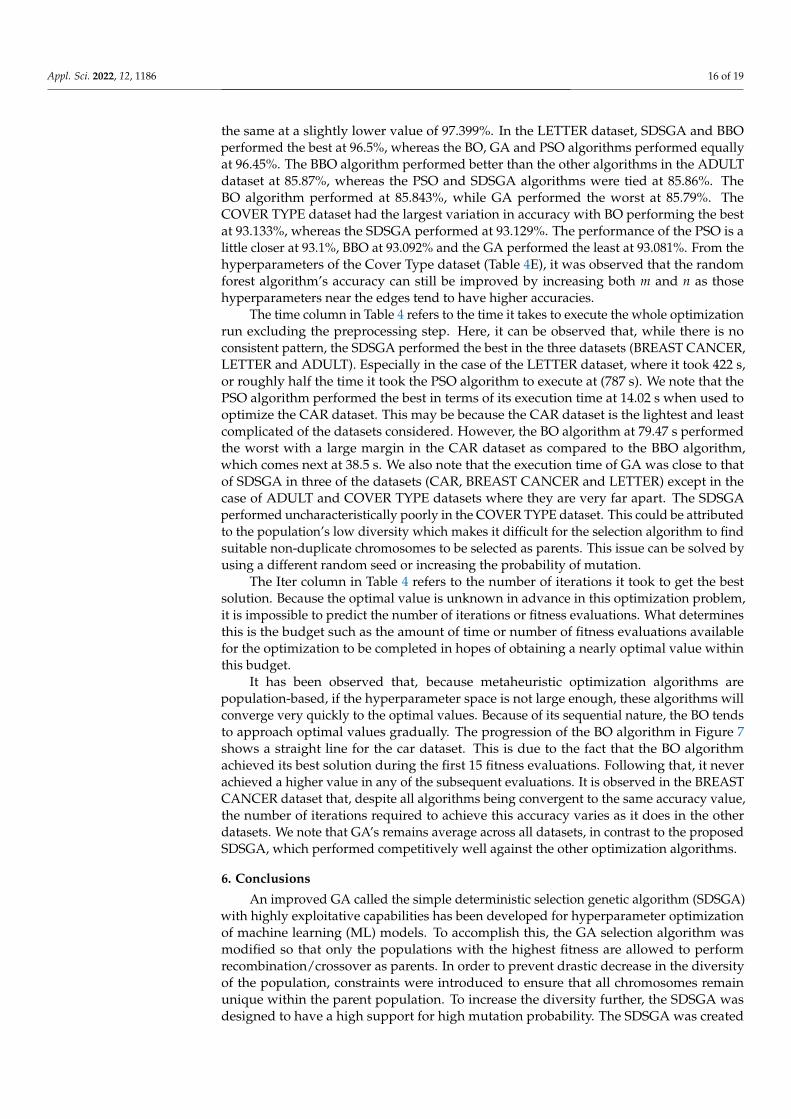
This section discusses how the proposed SDSGA performs when different percentagesP of the total population size were chosen as the number of parents, ranging from 10%to 90% with a 10% increment, when applied to the benchmark test functions, as well ashow the considered ML models, namely the random forest and the CNN performed whentrained on the MNIST and UCI datasets. Following Figure 4, the total number of best resultsrecorded across the entire benchmark functions by the SDSGA was 13 at both P = 20% and30% parent sizes.

The least performance was at P = 90%, which may be attributed to the fact that almostthe entire population was considered as parents, thus effectively reducing the chance forexploitation through recombination. Furthermore, the fact that the 20% and 30% parentsizes yielded the same number of the best outcomes shows that there were no statisticaldifferences between the two parent sizes. As a result, selecting any of the two parent sizeswill result in the same performance. Summarily, Figure 4 simply indicates that the SDSGAachieves the best performance in 13 of the benchmark functions when the parent size wasset to 20% and 30% of the total population.

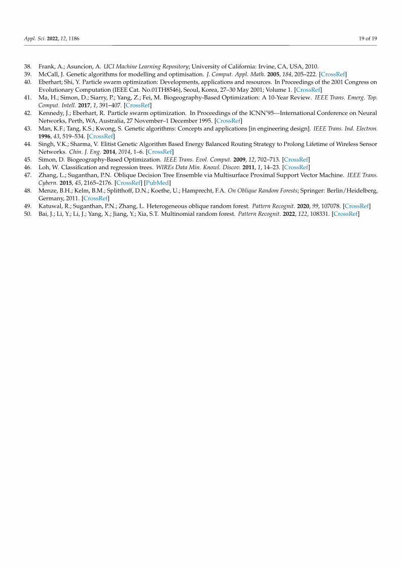
A similar study was performed on some UCI datasets, and it was discovered thata parent size of 20 and 30% yielded the best results when applied to different datasets,as shown in Figure 5. Nonetheless, we see a minor improvement in performance by theproposed SDSGA when a parent size of 20% was chosen and implemented on the LETTERand ADULT datasets as opposed to 30%. In the instance of the LETTER dataset, there wasa modest improvement in accuracy from around 96.5% for a parent size of 30% to about96.52% for the size of 20%, and, similarly, about 85.88% was recorded for the parent size of20% compared to 85.86% recorded for the 30% parent size (see Figure 5). We should pointout that the little change may not be statistically significant. As a result, the parent size ofeither 20 or 30% can be selected for evaluating the SDSGA.

Appl. Sci. 2022, 12, 1186 11 of 19

Benchmark Functions

12

10

v>8

•5

z 6

4

2

00.1 0 2 0 3 0 4 0,5 0 6 0 7 0 8 0 9 1

Number of parents (x100% of population)

Figure 4. Effect of varying the parent size.

Figure 5. Comparison of accuracy of the UCI datasets under varying parent population percentages.

5.2. Comparison and Evaluation of Optimization Algorithms on Benchmark Function

Table 2 shows the result of running the SDSGA on 17 benchmark functions andcomparing its performance with that of the GA, PSO and BBO algorithms. The lightgreen color in the table was used to highlight the best mean values per function, whilethe light brown color highlighted the highest standard deviation values. Table 2 showsthat the developed SDSGA performed better than the three compared algorithms in termsof accuracy in 65% of the benchmark functions. In some cases where the SDSGA did notperform as well as other algorithms used for comparison, the standard deviation showsthat the result does not deviate too far from the global optimum and that its results arestable across runs.

Appl. Sci. 2022, 12, 1186 12 of 19

Table 2. Result of comparison of metaheuristic algorithms on benchmark functions in 10D.

Algorithms

BBO GA PSO SDSGA

S/N Functions Global Sol Mean Std Mean Std Mean Std Mean Std

1 Ackley 0 5.81 × 10+00 7.96 × 10−01 2.20 × 10+00 6.19 × 10−01 1.41 × 10+01 8.04 × 10+00 1.53 × 10+00 2.70 × 10−01

2 DeJongsF1 0 1.86 × 10+01 1.35 × 10+01 5.96 × 10−01 4.76 × 10−01 3.62 × 10+00 1.44 × 10+00 4.96 × 10−01 5.88 × 10−01

3 DeJongsF2 0 2.54 × 10+04 2.03 × 10+04 1.07 × 10+03 8.16 × 10+02 3.27 × 10+03 3.90 × 10+03 6.53 × 10+02 4.13 × 10+02

4 Ellipsoid 0 7.67 × 10+05 4.95 × 10+05 6.94 × 10+03 8.76 × 10+03 1.67 × 10+05 1.29 × 10+05 1.16 × 10+04 2.54 × 10+04

5 Griewank 0 −6.90 × 10−01 5.30 × 10−02 −8.43 × 10−01 1.02 × 10−01 −4.62 × 10−01 2.31 × 10−01 −9.58 × 10−01 1.72 × 10−02

6 Hyper Ellipsodic 0 8.90 × 10+01 2.15 × 10+01 4.52 × 10+00 3.17 × 10+00 4.01 × 10+01 2.44 × 10+01 1.32 × 10+00 1.48 × 10+00

7 KTablet 0 4.96 × 10+04 1.18 × 10+04 9.35 × 10+02 1.13 × 10+03 1.39 × 10+04 7.81 × 10+03 1.09 × 10+03 1.40 × 10+03

8 Michalewicz −1.8013 −9.29 × 10+00 7.26 × 10−02 −9.31 × 10+00 9.63 × 10−02 −3.81 × 10+00 4.16 × 10−01 −9.43 × 10+00 1.74 × 10−01

9 Rastrigin 0 5.11 × 10+01 9.01 × 10+00 1.42 × 10+01 5.77 × 10+00 9.08 × 10+01 3.64 × 10+01 7.23 × 10+00 1.55 × 10+00

10 Rosenbrock 0 2.54 × 10+04 2.03 × 10+04 1.07 × 10+03 8.16 × 10+02 3.27 × 10+03 3.90 × 10+03 6.53 × 10+02 4.13 × 10+02

11 Schwefel −418.9829 −6.36 × 10+02 2.37 × 10−01 −6.36 × 10+02 9.51 × 10−02 −5.34 × 10+02 3.46 × 10+01 −6.36 × 10+02 1.12 × 10−01

12 Sphere 0 1.86 × 10+01 1.35 × 10+01 5.96 × 10−01 4.76 × 10−01 3.62 × 10+00 1.44 × 10+00 4.96 × 10−01 5.88 × 10−01

13 StyblinskiTang −391.66165 −180.32 1.13 × 10+02 −3.56 × 10+02 2.86 × 10+01 −2.99 × 10+02 4.58 × 10+01 −3.75 × 10+02 1.13 × 10+01

14 SumOfDiffPower 0 1.73 × 10+03 1.59 × 10+03 1.05 × 10+01 1.09 × 10+01 3.84 × 10+03 6.75 × 10+03 8.66 × 10−01 1.48 × 10+00

15 WeightedSphere 0 8.90 × 10+01 2.15 × 10+01 4.52 × 10+00 3.17 × 10+00 4.01 × 10+01 2.44 × 10+01 1.32 × 10+00 1.48 × 10+00

16 XinSheYang 0 3.56 × 10−03 4.00 × 10−04 2.84 × 10−03 7.37 × 10−04 1.60 × 10−01 9.39 × 10−02 3.01 × 10−03 1.02 × 10−03

17 Zakharov 0 −2.32 × 10+02 3.53 × 10+01 −2.52 × 10+02 4.65 × 10+01 −1.94 × 10+02 4.50 × 10+01 −1.91 × 10+02 5.81 × 10+01

Appl. Sci. 2022, 12, 1186 13 of 19

This is evident in the Griewank function results in Table 2 where it is noted that,while the SDSGA is not the best performing algorithm, its standard deviation is the best.Furthermore, when it came to optimizing the KTablet function, the GA came out on top interms of both mean best solution and standard deviation (=9.35 × 10+02, 1.13 × 10+03=).The SDSGA (=1.09 ×10+03, 1.40 × 10+03=) is not far from the GA when compared to bothBBO (4.96 × 10+04, 1.18 × 10+04) and PSO (1.39 × 10+04, 7.81 × 10+03).

5.3. CNN on the MNIST Dataset

This section summarizes the performance accuracy obtained when each of the opti-mization technique (SDSGA, GA, PSO, BBO and BO) were used to tune the HPs of the CNNon MNIST datasets. Due to the use of an early stopping strategy during the model training,if no further improvement is achieved, the execution time becomes a poor metric of evalua-tion. As an example, we discovered that, if the validation accuracy has not increased to 70%after three epochs of training, it fails to reach 90% even after 10 to 20 epochs. As a result,continuing to use such HP combinations wastes computational resources. Therefore, a bet-ter approach to measure the performance entailed selecting a baseline validation accuracyand comparing how many iterations it takes the algorithms to give such results. Table 3shows the results of optimizing the CNN model on the MNIST dataset. It was observedthat the BO algorithm performed the least with a value of 99.14%, which is slightly less thanthe PSO algorithm at 99.15% while the SDSGA performed the best with an average valueof about 99.2% (see Table 3). Similarly, the BBO algorithm recorded the next best in termsof performance with about 99.18%, while the GA performed at 99.17%. Furthermore, it wasdiscovered that the differences between the optimization algorithms are not significant.This could be due to the number of fitness evaluations chosen as 150 or it could be due tothe optimal accuracy of the ML model having plateaued around that value. Nonetheless,we discovered that increasing the number of fitness evaluations beyond 150 resulted in nofurther improvement in the results.

Table 3. Result of optimizing the CNN model on the MNIST dataset. The data have been prepared toshow the best accuracy so far.

PSO (%) GA (%) BBO (%) BO (%) SDSGA (%)

1 99.04 99.04 99 98.95 99.042 99.04 99.17 99.12 98.99 99.183 99.04 99.17 99.12 98.99 99.184 99.04 99.17 99.12 98.99 99.185 99.14 99.17 99.16 99.01 99.26 99.14 99.17 99.16 99.05 99.27 99.14 99.17 99.16 99.05 99.28 99.14 99.17 99.17 99.06 99.29 99.15 99.17 99.18 99.06 99.210 99.15 99.17 99.18 99.14 99.2

The BO algorithm performed the worst in terms of the number of fitness evaluationsrequired for the algorithms to reach optimal, with 99.14% at the tenth iteration. This meansthat the BO had performed 150 fitness evaluations to reach this value. The best performingalgorithm was the SDSGA, which achieved an accuracy of 99.2% at the fifth iteration. TheBBO algorithm performed the next best and achieved an accuracy of 99.18% at the ninthiteration, whereas the GA achieved 99.17% at the second iteration. The accuracy of theBBO algorithm shows that it performed better than the GA and PSO algorithm. Despitegradually improving, its results have been consistently optimal across all runs. Figure 6depicts a graph of the optimization algorithms’ accuracy as iteration progresses.

Appl. Sci. 2022, 12, 1186 14 of 19

Figure 6. Validation accuracy of CNN model as iteration progresses.

5.4. Random Forest on UCI Datasets

Table 4 shows the performance of the four metaheuristic algorithms when optimizingthe hyperparameters of random forest (RF) model based on four UCI datasets. The “Time”column shows the execution time, the column “Best Pos” shows the values of the besthyperparameters after the optimization run. The column “Best Sol” is the accuracy obtainedfor that run when using the best hyperparameters for that run. The “Iter” column showsthe number of iterations it takes for the algorithm to arrive at that accuracy. The variationof the prediction accuracies for all the optimization algorithms is shown in Figure 7.

Figure 7. Prediction accuracy for the different algorithms under the different UCI datasets.

Appl. Sci. 2022, 12, 1186 15 of 19

Table 4. Performance of the metaheuristic-based algorithms on RF trained on four differentUCI datasets.

A: CAR

Algorithm Time (s) Best Pos Best Sol (%) Iter

PSO 14.02 [174, 6] 97.399 5GA 27.65 [163, 6] 97.399 6BBO 38.5 [120, 6] 97.399 2BO 79.47 [129, 6] 97.688 1

SDSGA 22.48 [117, 6] 97.688 3

B: BREAST CANCER

Algorithm Time (s) Best Pos Best Sol (%) Iter

PSO 60.43 [129, 7] 98.246 3GA 47.95 [143, 7] 98.246 7BBO 62.92 [118, 16] 98.246 4BO 106.4 [68, 20] 98.246 5

SDSGA 41.37 [124, 7] 98.246 2

C: LETTER

Algorithm Time (s) Best Pos Best Sol (%) Iter

PSO 787.68 [198, 5] 96.45 3GA 427.81 [141, 5] 96.45 5BBO 599.96 [91, 4] 96.5 7BO 616.72 [141, 5] 96.45 10

SDSGA 422.75 [85, 4] 96.5 2

D: ADULT

Algorithm Time (s) Best Pos Best Sol (%) Iter

PSO 763.43 [184, 15] 85.86 4GA 780 [138, 15] 85.79 3BBO 953.09 [193, 15] 85.87 8BO 942.51 [183, 15] 85.843 4

SDSGA 655.41 [184, 15] 85.86 7

E: Cover Type

Algorithm Time (s) Best Pos Best Sol (%) Iter

PSO 11,847.65 [198, 19] 93.1 8GA 5481.84 [155, 18] 93.081 6BBO 11,721.25 [193, 18] 93.092 7BO 13,437.37 [188, 20] 93.133 3

SDSGA 10,907.01 [194, 20] 93.129 6

We present in Table 4 the results obtained when training the RF model on five UCIdatasets using the BO, SDSGA, GA, PSO and BBO algorithms to tune the HPs. In somecases, the best solution obtained by each optimization algorithm (BO, SDSGA, GA, PSO andBBO) was the same as demonstrated by the Breast Cancer dataset, where all optimizationalgorithms achieved an accuracy of 98.246% despite being obtained under different HPsvalues (see Table 4B). This is because the multiple hyperparameter combinations producedthe same validation accuracy in this problem. Because the outcome is heavily dependent onthe initial population, this can have a significant impact on the efficiency of metaheuristicoptimization algorithms.

In the CAR dataset (Table 4A), it is noticed that both the BO and SDSGA algorithmsperformed the best at 97.688% while the rest of the optimization algorithms performed

Appl. Sci. 2022, 12, 1186 16 of 19

the same at a slightly lower value of 97.399%. In the LETTER dataset, SDSGA and BBOperformed the best at 96.5%, whereas the BO, GA and PSO algorithms performed equallyat 96.45%. The BBO algorithm performed better than the other algorithms in the ADULTdataset at 85.87%, whereas the PSO and SDSGA algorithms were tied at 85.86%. TheBO algorithm performed at 85.843%, while GA performed the worst at 85.79%. TheCOVER TYPE dataset had the largest variation in accuracy with BO performing the bestat 93.133%, whereas the SDSGA performed at 93.129%. The performance of the PSO is alittle closer at 93.1%, BBO at 93.092% and the GA performed the least at 93.081%. From thehyperparameters of the Cover Type dataset (Table 4E), it was observed that the randomforest algorithm’s accuracy can still be improved by increasing both m and n as thosehyperparameters near the edges tend to have higher accuracies.

The time column in Table 4 refers to the time it takes to execute the whole optimizationrun excluding the preprocessing step. Here, it can be observed that, while there is noconsistent pattern, the SDSGA performed the best in the three datasets (BREAST CANCER,LETTER and ADULT). Especially in the case of the LETTER dataset, where it took 422 s,or roughly half the time it took the PSO algorithm to execute at (787 s). We note that thePSO algorithm performed the best in terms of its execution time at 14.02 s when used tooptimize the CAR dataset. This may be because the CAR dataset is the lightest and leastcomplicated of the datasets considered. However, the BO algorithm at 79.47 s performedthe worst with a large margin in the CAR dataset as compared to the BBO algorithm,which comes next at 38.5 s. We also note that the execution time of GA was close to thatof SDSGA in three of the datasets (CAR, BREAST CANCER and LETTER) except in thecase of ADULT and COVER TYPE datasets where they are very far apart. The SDSGAperformed uncharacteristically poorly in the COVER TYPE dataset. This could be attributedto the population’s low diversity which makes it difficult for the selection algorithm to findsuitable non-duplicate chromosomes to be selected as parents. This issue can be solved byusing a different random seed or increasing the probability of mutation.

The Iter column in Table 4 refers to the number of iterations it took to get the bestsolution. Because the optimal value is unknown in advance in this optimization problem,it is impossible to predict the number of iterations or fitness evaluations. What determinesthis is the budget such as the amount of time or number of fitness evaluations availablefor the optimization to be completed in hopes of obtaining a nearly optimal value withinthis budget.

It has been observed that, because metaheuristic optimization algorithms arepopulation-based, if the hyperparameter space is not large enough, these algorithms willconverge very quickly to the optimal values. Because of its sequential nature, the BO tendsto approach optimal values gradually. The progression of the BO algorithm in Figure 7shows a straight line for the car dataset. This is due to the fact that the BO algorithmachieved its best solution during the first 15 fitness evaluations. Following that, it neverachieved a higher value in any of the subsequent evaluations. It is observed in the BREASTCANCER dataset that, despite all algorithms being convergent to the same accuracy value,the number of iterations required to achieve this accuracy varies as it does in the otherdatasets. We note that GA’s remains average across all datasets, in contrast to the proposedSDSGA, which performed competitively well against the other optimization algorithms.

6. Conclusions

An improved GA called the simple deterministic selection genetic algorithm (SDSGA)with highly exploitative capabilities has been developed for hyperparameter optimizationof machine learning (ML) models. To accomplish this, the GA selection algorithm wasmodified so that only the populations with the highest fitness are allowed to performrecombination/crossover as parents. In order to prevent drastic decrease in the diversityof the population, constraints were introduced to ensure that all chromosomes remainunique within the parent population. To increase the diversity further, the SDSGA wasdesigned to have a high support for high mutation probability. The SDSGA was created

Appl. Sci. 2022, 12, 1186 17 of 19

to allow for high accuracy search for hyperparameters in machine learning models whentime is limited. The optimization results of the proposed method on benchmark functionswere compared with that of the GA, PSO and BBO algorithms, and the results obtainedshow that, overall, the SDSGA performed better than the other algorithms in 65% of thebenchmark functions in terms of mean accuracy, albeit marginally. It is worth noting thatthe BBO algorithm performed the worst in all of the test functions evaluated herein. This isnot necessarily due to the BBO being inferior as other factors such as the type of functionand parameters used may have contributed for performance degradation. The comparisonof the SDSGA with other optimization algorithms including the BO algorithm showedthat our improved GA performed well, particularly in optimizing the CNN model on theMNIST dataset with an accuracy of 99.2%. For the case of the random forest model, ourSDSGA performed marginally better than the other algorithms in most cases except infew cases where the PSO performed best, particularly on the CAR dataset in terms of itsexecution time. Despite this, we note that the better performances of our method, albeitmarginally, were achieved at faster computing times than the other methods, emphasizingthe proposed method’s advantage. It is possible to compare the SDSGA with other popularmetaheuristic algorithms such as the artificial bee colony (ABC), differential evolution(DE), covariance matrix adaptation evolutionary strategy (CMA-ES), and the grey wolfoptimization (GWO) algorithms for hyperparameter tuning of ML models, which servesto provide a direction for further research. Additionally, its consistency can be tested onhigh-dimensional spaces and multi-objective problems to determine how well it performsin these environments.

Author Contributions: I.D.R., H.B.-S., I.J.U., A.J.O., M.A.A. and A.T.S. contributed equally to thiswork. Conceptualization, H.B.-S., I.D.R., I.J.U. and A.J.O.; methodology, H.B.-S. and I.D.R.; writing—original draft preparation, H.B.-S. and I.D.R.; writing—review and editing, H.B.-S., A.J.O., M.A.A.and A.T.S.; supervision, H.B.-S., A.J.O., M.A.A. and A.T.S.; funding acquisition, M.A.A. All authorshave read and agreed to the published version of the manuscript.

Funding: This research received no external funding.

Institutional Review Board Statement: Not applicable.

Informed Consent Statement: Not applicable.

Data Availability Statement: Not applicable.

Conflicts of Interest: The authors declare no conflict of interest. The funders had no role in the designof the study; in the collection, analyses, or interpretation of data; in the writing of the manuscript, orin the decision to publish the results.

References1. Khurana, D.; Koli, A.; Khatter, K.; Singh, S. Natural Language Processing: State of The Art, Current Trends and Challenges. arXiv

2017, arXiv:1708.05148.2. Friedman, C.; Rindflesch, T.C.; Corn, M. Natural language processing: State of the art and prospects for significant progress, a

workshop sponsored by the National Library of Medicine. J. Biomed. Inform. 2013, 46, 765–773. [CrossRef] [PubMed]3. Khan, Z.A.; Feng, Z.; Irfan Uddin, M.; Mast, N.; Shah, S.A.A.; Imtiaz, M.; Al-Khasawneh, M.A.; Mahmoud, M. Optimal policy

learning for disease prevention using reinforcement learning. Sci. Prog. 2020, 2020, 1–13. [CrossRef]4. Mendoza, H.; Klein, A.; Feurer, M.; Springenberg, J.T.; Hutter, F. Towards Automatically-Tuned Neural Networks. In Automated

Machine Learning; Springer, Cham, Switzerland, 2016.5. Thornton, C.; Hutter, F.; Hoos, H.H.; Leyton-Brown, K. Auto-WEKA: Combined selection and hyperparameter optimization of

classification algorithms. In Proceedings of the ACM SIGKDD International Conference on Knowledge Discovery and DataMining, Chicago, IL, USA, 11–14 August 2013; Volume Part F128815, pp. 847–855. [CrossRef]

6. Loshchilov, I.; Schoenauer, M.; Sebag, M. BI-Population CMA-ES Algorithms with Surrogate Models and Line Searches. InProceedings of the 15th Annual Conference Companion on Genetic and Evolutionary Computation, Amsterdam, The Netherlands,6–10 July 2013; pp. 1177–1184. [CrossRef]

7. Yu, T.; Zhu, H. Hyper-Parameter Optimization: A Review of Algorithms and Applications. arXiv 2020, arXiv:2003.05689.8. Levesque, J.C.; Durand, A.; Gagne, C.; Sabourin, R. Bayesian optimization for conditional hyperparameter spaces. In Proceedings

of the International Joint Conference on Neural Networks, Anchorage, AK, USA, 14–19 May 2017; pp. 286–293. [CrossRef]

Appl. Sci. 2022, 12, 1186 18 of 19

9. Bergstra, J.; Bengio, Y. Random search for hyper-parameter optimization. J. Mach. Learn. Res. 2012, 13, 281–305.10. Bergstra, J.; Yamins, D.; Cox, D. Hyperopt: A Python Library for Optimizing the Hyperparameters of Machine Learning Algorithms. In

Proceedings of the 12th Python in Science Conference, Austin, TX, USA, 24–29 June 2013; pp. 13–19. [CrossRef]11. Wu, J.; Chen, X.Y.; Zhang, H.; Xiong, L.D.; Lei, H.; Deng, S.H. Hyperparameter optimization for machine learning models based

on Bayesian optimization. J. Electron. Sci. Technol. 2019, 17, 26–40. [CrossRef]12. Loshchilov, I.; Hutter, F. CMA-ES for Hyperparameter Optimization of Deep Neural Networks. arXiv 2016, arXiv:1604.07269.13. Bergstra, J.; Bardenet, R.; Bengio, Y.; Kégl, B. Algorithms for hyper-parameter optimization. Adv. Neural Inf. Process. Syst. 2011, 24,

2546–2554.14. Wang, J.; Xu, J.; Wang, X. Combination of Hyperband and Bayesian Optimization for Hyperparameter Optimization in Deep

Learning. arXiv 2018, arXiv:1801.01596.15. Jin, H.; Song, Q.; Hu, X. Auto-keras: An efficient neural architecture search system. In Proceedings of the ACM SIGKDD

International Conference on Knowledge Discovery and Data Mining, Anchorage, AK, USA, 4–8 August 2019; pp. 1946–1956.[CrossRef]

16. Snoek, J.; Larochelle, H.; Adams, R.P. Practical Bayesian optimization of machine learning algorithms. Adv. Neural Inf. Process.Syst. 2012, 4, 2951–2959.

17. Li, L.; Jamieson, K.; Rostamizadeh, A.; Gonina, E.; Hardt, M.; Recht, B.; Talwalkar, A. A System for Massively ParallelHyperparameter Tuning. arXiv 2018, arXiv:1810.05934.

18. Li, L.; Jamieson, K.; DeSalvo, G.; Rostamizadeh, A.; Talwalkar, A. Hyperband: A novel bandit-based approach to hyperparameteroptimization. J. Mach. Learn. Res. 2018, 18, 6765–6816.

19. Jamieson, K.; Talwalkar, A. Non-stochastic best arm identification and hyperparameter optimization. In Proceedings of the 19thInternational Conference on Artificial Intelligence and Statistics, AISTATS 2016, Cadiz, Spain, 9–11 May 2016; pp. 240–248.

20. Klein, A.; Falkner, S.; Bartels, S.; Hennig, P.; Hutter, F. Fast Bayesian hyperparameter optimization on large datasets. Electron. J.Stat. 2017, 11, 4945–4968. [CrossRef]

21. Friedrichs, F.; Igel, C. Evolutionary tuning of multiple SVM parameters. Neurocomputing 2005, 64, 107–117. [CrossRef]22. Li, Y.; Zhang, Y. Hyper-parameter estimation method with particle swarm optimization. arXiv 2020, arXiv:2011.11944.23. Bacanin, N.; Bezdan, T.; Tuba, E.; Strumberger, I.; Tuba, M. Optimizing convolutional neural network hyperparameters by

enhanced swarm intelligence metaheuristics. Algorithms 2020, 13, 67. [CrossRef]24. Han, J.; Gondro, C.; Reid, K.; Steibel, J.P. Heuristic hyperparameter optimization of deep learning models for genomic prediction.

G3 Genes Genomes Genet. 2021, 11, 398800. [CrossRef]25. Lorenzo, P.R.; Nalepa, J.; Ramos, L.S.; Pastor, J.R. Hyper-parameter selection in deep neural networks using parallel particle

swarm optimization. In Proceedings of the Genetic and Evolutionary Computation Conference Companion, Berlin, Germany,15–19 July 2017; pp. 1864–1871. [CrossRef]

26. Mantovani, R.G.; Horvath, T.; Cerri, R.; Vanschoren, J.; De Carvalho, A.C. Hyper-Parameter Tuning of a Decision Tree InductionAlgorithm. In Proceedings of the 2016 5th Brazilian Conference on Intelligent Systems (BRACIS), Recife, Brazil, 9–12 October2016; pp. 37–42. [CrossRef]

27. Tani, L.; Rand, D.; Veelken, C.; Kadastik, M. Evolutionary algorithms for hyperparameter optimization in machine learning forapplication in high energy physics. Eur. Phys. J. C. 2021, 81, 1–9. [CrossRef]

28. Feurer, M.; Klein, A.; Eggensperger, K.; Springenberg, J.T.; Blum, M.; Hutter, F. Auto-sklearn: Efficient and Robust AutomatedMachine Learning. In Automated Machine Learning; Springer International Publishing: Berlin, Germany, 2019; pp. 113–134.[CrossRef]

29. Kotthoff, L.; Thornton, C.; Hoos, H.H.; Hutter, F.; Leyton-Brown, K. Auto-WEKA: Automatic Model Selection and HyperparameterOptimization in WEKA. In Automated Machine Learning; Springer International Publishing: Berlin, Germany, 2019; pp. 81–95.[CrossRef]

30. Zimmer, L.; Lindauer, M.; Hutter, F. Auto-Pytorch: Multi-Fidelity MetaLearning for Efficient and Robust AutoDL. IEEE Trans.Pattern Anal. Mach. Intell. 2021, 43, 3079–3090. [CrossRef]

31. Bhandari, D.; Murthy, C.A.; Pal, S.K. Genetic Algorithm with Elitist Model and ITS Convergence. Int. J. Pattern Recognit. Artif.Intell. 1996, 10, 731–747. [CrossRef]

32. Liang, Y.; Leung, K.S. Genetic Algorithm with adaptive elitist-population strategies for multimodal function optimization. Appl.Soft Comput. 2011, 11, 2017–2034. [CrossRef]

33. Aibinu, A.M.; Bello Salau, H.; Rahman, N.A.; Nwohu, M.N.; Akachukwu, C.M. A novel Clustering based Genetic Algorithm forroute optimization. Eng. Sci. Technol. Int. J. 2016, 19, 2022–2034. [CrossRef]

34. Bello-Salau, H.; Aibinu, A.M.; Wang, Z.; Onumanyi, A.J.; Onwuka, E.N.; Dukiya, J.J. An optimized routing algorithm for vehiclead-hoc networks. Eng. Sci. Technol. Int. J. 2019, 22, 754–766. [CrossRef]

35. Allawi, Z.T.; Ibraheem, I.K.; Humaidi, A.J. Fine-tuning meta-heuristic algorithm for global optimization. Processes 2019, 7, 657.[CrossRef]

36. Arıcı, F.; Kaya, E. Comparison of Meta-heuristic Algorithms on Benchmark Functions. Acad. Perspect. Procedia 2019, 2, 508–517.[CrossRef]

37. LeCun, Y.; Bottou, L.; Bengio, Y.; Haffner, P. Gradient-based learning applied to document recognition. Proc. IEEE 1998,86, 2278–2323. [CrossRef]

Appl. Sci. 2022, 12, 1186 19 of 19

38. Frank, A.; Asuncion, A. UCI Machine Learning Repository; University of California: Irvine, CA, USA, 2010.39. McCall, J. Genetic algorithms for modelling and optimisation. J. Comput. Appl. Math. 2005, 184, 205–222. [CrossRef]40. Eberhart; Shi, Y. Particle swarm optimization: Developments, applications and resources. In Proceedings of the 2001 Congress on

Evolutionary Computation (IEEE Cat. No.01TH8546), Seoul, Korea, 27–30 May 2001; Volume 1. [CrossRef]41. Ma, H.; Simon, D.; Siarry, P.; Yang, Z.; Fei, M. Biogeography-Based Optimization: A 10-Year Review. IEEE Trans. Emerg. Top.

Comput. Intell. 2017, 1, 391–407. [CrossRef]42. Kennedy, J.; Eberhart, R. Particle swarm optimization. In Proceedings of the ICNN’95—International Conference on Neural

Networks, Perth, WA, Australia, 27 November–1 December 1995. [CrossRef]43. Man, K.F.; Tang, K.S.; Kwong, S. Genetic algorithms: Concepts and applications [in engineering design]. IEEE Trans. Ind. Electron.

1996, 43, 519–534. [CrossRef]44. Singh, V.K.; Sharma, V. Elitist Genetic Algorithm Based Energy Balanced Routing Strategy to Prolong Lifetime of Wireless Sensor

Networks. Chin. J. Eng. 2014, 2014, 1–6. [CrossRef]45. Simon, D. Biogeography-Based Optimization. IEEE Trans. Evol. Comput. 2009, 12, 702–713. [CrossRef]46. Loh, W. Classification and regression trees. WIREs Data Min. Knowl. Discov. 2011, 1, 14–23. [CrossRef]47. Zhang, L.; Suganthan, P.N. Oblique Decision Tree Ensemble via Multisurface Proximal Support Vector Machine. IEEE Trans.

Cybern. 2015, 45, 2165–2176. [CrossRef] [PubMed]48. Menze, B.H.; Kelm, B.M.; Splitthoff, D.N.; Koethe, U.; Hamprecht, F.A. On Oblique Random Forests; Springer: Berlin/Heidelberg,

Germany, 2011. [CrossRef]49. Katuwal, R.; Suganthan, P.N.; Zhang, L. Heterogeneous oblique random forest. Pattern Recognit. 2020, 99, 107078. [CrossRef]50. Bai, J.; Li, Y.; Li, J.; Yang, X.; Jiang, Y.; Xia, S.T. Multinomial random forest. Pattern Recognit. 2022, 122, 108331. [CrossRef]