BAMBERGER BEITRÄGE ZURWIRTSCHAFTSINFORMATIK UND ANGEWANDTEN INFORMATIK

ISSN 0937-3349

Nr. 94/August 2014

Grounding Synchronous DeterministicConcurrency in Sequential

Programming

Joaquín Aguado, Michael Mendler,Reinhard von Hanxleden, Insa Fuhrmann

FAKULTÄT FÜRWIRTSCHAFTSINFORMATIK UND ANGEWANDTE INFORMATIK

OTTO-FRIEDRICH-UNIVERSITÄT BAMBERG

1

Grounding Synchronous DeterministicConcurrency in Sequential Programming

Joaquın Aguado∗, Michael Mendler∗, Reinhard von Hanxleden†, Insa Fuhrmann†

∗Faculty of Information Systems and Applied Computer Sciences,Bamberg University, Germany; E-mail: {michael.mendler, joaquin.aguado}@uni-bamberg.de

†Department of Computer Science,Kiel University, Germany; E-mail: {rvh, ima}@informatik.uni-kiel.de

Abstract

In this report, we introduce an abstract interval domain I(D,P) and associated fixed pointsemantics for reasoning about concurrent and sequential variable accesses within a synchronouscycle-based model of computation. The interval domain captures must (lower bound) and cannot(upper bound) information to approximate the synchronisation status of variables consisting of avalue status D and an init status P. We use this domain for a new behavioural definition of Berry’scausality analysis for Esterel. This gives a compact and uniform understanding of Esterel-styleconstructiveness for shared-memory multi-threaded programs. Using this new domain-theoreticcharacterisation we show that Berry’s constructive semantics is a conservative approximation ofthe recently proposed sequentially constructive (SC) model of computation. We prove that everyBerry-constructive program is sequentially constructive, i.e., deterministic and deadlock-free undersequentially admissible scheduling. This gives, for the first time, a natural interpretation of Berry-constructiveness for main-stream imperative programming in terms of scheduling, where previousresults were cast in terms of synchronous circuits. It also opens the door to a direct mapping ofEsterel’s signal mechanism into boolean variables that can be set and reset arbitrarily within a tick.We illustrate the practical usefulness of this mapping by discussing how signal reincarnation ishandled efficiently by this transformation, which is of complexity that is linear in program size, incontrast to earlier techniques that had, at best, potentially quadratic overhead.

Keywords: Concurrency, determinism, constructiveness, Mealy reactive systems, synchronousprogramming, Esterel.

I. INTRODUCTION

If traditional main-stream programming was largely single-threaded and sequential, thenew multi-core processing age raises the incentives for concurrent programming. However,multi-threaded, shared memory programming is notoriously difficult because of data races(write-write, read-write conflicts) which jeopardize the functional correctness and predictabilityof program behavior. The main-stream answer to avoid the non-determinism are elementarysynchronization primitives, such as monitors, semaphores and locks. Stemming from the earlydays of concurrent programming, these general-purpose operators are safe in the hands of anexpert but not necessarily in the hands of the novice [23], [27].

This work is part of the PRETSY project and supported by the German National Research Council DFG (HA 4407/6-1,ME 1427/6-1). Preliminary result were presented at Synchron 2013, 19th November 2013, Dagstuhl, Germany, and at theEuropean Symposium on Programming ESOP’14, 9th April 2014, Grenoble, France.

An approach which does not rely on “spaghetti-style” synchronization through low-levelprimitives, is the synchronous model of computation (SMoC). SMoC is a disciplined synchro-nization regime based on logical clocks and signals as the key synchronization mechanisms.To ensure determinism and bounded response, it enforces a strict cycle-based communicationpattern between concurrent threads, which abstracts the principle of deterministic input-outputMealy machines.

A synchronous computation, consisting of a system and an environment, is generallydescribed by an ordered sequence of reactions, each one occurring at a global clock tickacting as a synchronization barrier. In a synchronous program, these ticks are derived fromexplicit clocks, as in Lustre [14] or Signal [22], or from statements such as Esterel’s [10]pause which establish precisely identifiable configurations or global states of the system inquestion. What happens, then, between two ticks, i.e., within a macro-step, is a change fromone system configuration to the next. This change results from the combined (concurrent orinterleaved) execution of the system’s individual statements, or micro-steps, that are scheduledand active during the current macro-step. The environment, in turn, perceives macro-stepsas atomic (instantaneous) computations during which it cannot intervene at all. Instead, theenvironment’s observations and interactions can only occur at the places delimited by thepause, namely stable configurations. This modeling is known as the Synchrony Hypothesis.

This abstraction has led to the family of synchronous languages [6], which have been usedsuccessfully in particular in safety-critical embedded systems, such as avionics applications.The synchrony abstraction naturally leads to a fixed-point semantics, where all variables thatare computed as part of a reaction have a unique value throughout the reaction. In data-floworiented synchronous languages, such as Lustre or SCADE [20], this means that for eachvariable, there must be a unique defining equation, leading to a declarative programming style.In imperative, control-flow oriented languages, such as Esterel, SyncCharts [4] or Quartz [39],the synchrony abstraction means that a signal—a special type of variable, discussed in detaillater—must not be modified after it has been read (“write-before-read protocol”). This protocolleads to the notion of constructiveness, also referred to as causality; a program is consideredconstructive if and only if this “write-before-read” protocol is neither too stringent to createdeadlocks, nor too lax to permit non-determinism. Programs that are not constructive mustbe rejected at compile time. The possibility for compile-time reasoning, which eliminatesrun-time deadlock and non-determinism, is one of the strengths of synchronous programming.

The synchrony abstraction has proven to be useful in practice. Its sound mathematicalbasis allows formal reasoning and verification. However, the construction principles used sofar mainly in synchronous languages can be naturally generalized and mapped to familiar,sequential programming concepts as used in C or Java. This not only allows a fresh lookat existing synchronous languages, including more efficient compilation strategies, but alsoleads to natural extensions that facilitate a familiar, sequential programming style. In thisvein, we recently introduced the notion of sequential constructiveness (SC) [46], [47], [48]to integrate SMoC with main-stream sequential languages such as Java or C. The idea is toreconstruct signals and their synchronization properties in terms of variables and schedulingconstraints on variable accesses. SC leaves more control to the programmer than traditionalSMoC would permit. SC exploits the fact that the program-prescribed sequencing of statementscan typically be implemented reliably by the compiler on the run-time system. This assumptionis not usually made in traditional SMoC which targets sequential hardware circuits as therun-time architecture. The SMoC advantage is that it offers more robustness with respect to the

2

admissible run-time models regarding reordering of statements, while SC is more permissiveand more flexible to use in the context of sequential programming.

Contributions. In this report, we investigate the formal semantical relationship between SCand SMoC (restricted to boolean programs) which has been discussed only informally before.Our results offer an interpretation of SC as a clocked scheduling protocol which, within asingle clock tick, supports arbitrary sequences of concurrent “init;update;read” accesses onshared variables. This reduces the number of required clock cycles compared to SMoC whichdoes not permit such repetitions. The contributions of this report are as follows:• We introduce the class of ∆0-constructive programs for multi-threaded shared memory

programs in which one concurrent “init;update;read”1 cycle is permitted and initializationsare under the programmer’s control. This generalizes Berry’s notion of constructivenessfor Esterel which we identify as a relaxation ∆1 of the ∆0 class in which all initializationsare implicit. We call ∆1 the class of Berry-constructive programs and ∆0 the stronglyBerry-constructive programs.

• We present both levels of constructiveness ∆0 and ∆1 as approximations to SC in the formof fixed point analyses in abstract domains of signal statuses. Concretely, ∆1 is equivalentto ternary analysis, which is known to be related to delay-insensitive boolean circuits,while ∆0 refines this naturally in a domain of approximation intervals I(D,P). Thisbrings a novel characterization of Berry’s must-cannot analysis that suggests extensionsto other data types.

• We show that both ∆0 and ∆1 are properly included in SC, referred to as ∆∗, whichpermits arbitrarily many repetitions of concurrent “init;update;read” cycles. This provesformally that (pure) SC is indeed a conservative extension of (pure) Esterel thus solvingan open problem [47].

• Finally, to illustrate the usefulness of SC (beyond ∆1), we show by example how twoinitializations during one tick implements efficiently some forms of signal reincarnation,known in SMoC as the “schizophrenia” problem. Ample earlier work suggests thatcode transformations for separating signal incarnations require at least quadratic-sizecode duplication [8], [38], [42]. We here argue that this is a consequence of working at∆1-level. We show that in ∆∗ a code transformation that separates signal incarnationscan be implemented in linear size.

Overview. We start in Sec. II with a discussion on how synchronous signals can be representedusing variables in shared memory multi-threading. We illustrate the SC model of synchronouscomputation and its role for the proper sequencing of signal initialization. Sec. III providesthe technical setup for our results and the operational reference semantics. This includes thedefinition of a kernel language for pure boolean programs (Sec. III-A), the formal definitionof its operational semantics of micro steps and macro steps (Sec. III-B) and the notion ofsequential constructiveness, here called ∆∗-constructiveness (Sec. III-C). In Sec. IV we presentan approximation of ∆∗-constructiveness in terms of a denotational fixed point semantics. Wefirst introduce the semantic information domains on which the fixed point is approximated.This consists of status information on variables (Sec. IV-A) inducing an associated notion ofsignal environment (Sec. IV-B) and a domain specifying the completion status of a program(Sec. IV-C). Finally, the class of strongly Berry-constructive, or ∆0-constructive programs,is defined (Sec. IV-D). Sec. V then contains our main result. We prove that the fixed point

1We use the semicolon “init;update;read” rather than a hyphen “init-update-read” to stress the strict sequential orderingbetween the phases.

3

semantics is sound with respect to the operational semantics, i.e., that ∆0-constructivenessprovides a conservative over-approximation of ∆∗-constructiveness. In Sec. 13 we study therelationship between ∆0 and Berry’s notion of constructiveness introduced for Esterel, whichwe formulate as a special case of the ∆0 semantics, called ∆1. Finally, Sec. VII sums up theresults and comments on related work.

II. GROUNDING SYNCHRONOUS SIGNALS IN SEQUENTIAL VARIABLES

Before a formal treatment of the subject matter in later sections, we will set the stage bycomparing signals, a key SMoC concept to achieve deterministic concurrency, with variables,familiar from sequential languages as C and Java.

A. Signals in a sequential settingA SMoC signal comprises a status and a value. The status of a signal is per default absent

in each tick and its value set to an initial value. If and when a signal is emitted its statusbecomes present in the current tick. With each emission the signal’s value is updated, typicallyby way of an (associative and commutative) combination function. As soon as a configurationis reached in which the value of a variable is never updated again, its value can be read. Anyreading of a signal’s value or reacting to its absent status has to wait for stabilization. On theother hand, a reaction to the present status (as opposed to reading its value) can safely takeplace after the first emission. This synchronization protocol, characteristic to all Esterel-styleSMoCs, corresponds to a single “init;update;read” cycle which enforces deterministic reactions.Programs which are also deadlock free are called causal or constructive.

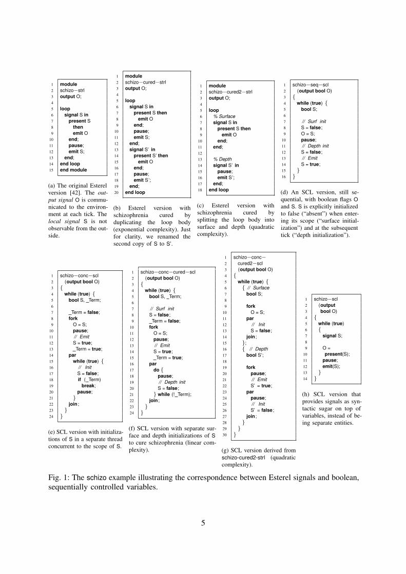
Fig. 1a shows schizo-strl, an example of how signals are used in Esterel, taken from Tardieuand de Simone [42]. In the initial tick, the present S statement in lines 7–9 emits O if S ispresent. This is the only possible emission of O in the first tick; hence, as S cannot be emitted,O is not emitted. The pause statement in line 11 then terminates the current tick. In the nexttick, control resumes in line 12 where the emit S makes S present, however, the local scopeof S is left immediately afterwards with the end in line 13. When, after looping around, thescope of S is re-entered in line 6, a fresh instance of S is installed that has not been emittedyet, so the test for the presence of S in lines 7–9 fails again.

Signals that may become absent and present in the same tick, such as S in schizo-strl, arecalled schizophrenic. Schizophrenic signals bring a risk for non-determinism, for example,when synthesizing hardware, as signal wires must have a stable voltage. Thus a number ofstrategies have been proposed to eliminate schizophrenia by code transformations [8], [38],[42]. These transformations essentially duplicate loop bodies when they contain local signalscopes that might be left and re-entered in the same tick, as illustrated in schizo-cured-strl inFig. 1b. This approach “cures” the schizophrenia problem, but could lead to an exponentialcode increase.

This can be improved by distinguishing surface and depth [8] of a (compound) statementS, where S in this case is the body of the loop. The surface is the part that can be executedin the same tick when entering S, and the depth is the part of S that can be executed insubsequent ticks. The basic idea is to split S into a surface copy SC and a depth copy SD,where pauses in SC are replaced by a “gotopause” that transfers control to the correspondingpause in SD [42]. The schizo-cured2-strl version in Fig. 1c illustrates this approach, where in

4

1 module2 schizo−strl3 output O;45 loop6 signal S in7 present S8 then9 emit O

10 end;11 pause;12 emit S;13 end;14 end loop15 end module

(a) The original Esterelversion [42]. The out-put signal O is commu-nicated to the environ-ment at each tick. Thelocal signal S is notobservable from the out-side.

1 module2 schizo−cured−strl3 output O;45 loop6 signal S in7 present S then8 emit O9 end;

10 pause;11 emit S;12 end;13 signal S’ in14 present S’ then15 emit O16 end;17 pause;18 emit S’;19 end;20 end loop

(b) Esterel version withschizophrenia cured byduplicating the loop body(exponential complexity). Justfor clarity, we renamed thesecond copy of S to S’.

1 module2 schizo−cured2−strl3 output O;45 loop6 % Surface7 signal S in8 present S then9 emit O

10 end;11 end;1213 % Depth14 signal S’ in15 pause;16 emit S’;17 end;18 end loop

(c) Esterel version withschizophrenia cured bysplitting the loop body intosurface and depth (quadraticcomplexity).

1 schizo−seq−scl2 (output bool O)3 {4 while (true) {5 bool S;67 // Surf init8 S = false;9 O = S;

10 pause;11 // Depth init12 S = false;13 // Emit14 S = true;15 }16 }

(d) An SCL version, still se-quential, with boolean flags Oand S. S is explicitly initializedto false (“absent”) when enter-ing its scope (“surface initial-ization”) and at the subsequenttick (“depth initialization”).

1 schizo−conc−scl2 (output bool O)3 {4 while (true) {5 bool S, Term;67 Term = false;8 fork9 O = S;

10 pause;11 // Emit12 S = true;13 Term = true;14 par15 while (true) {16 // Init17 S = false;18 if ( Term)19 break;20 pause;21 }22 join ;23 }24 }

(e) SCL version with initializa-tions of S in a separate threadconcurrent to the scope of S.

1 schizo−conc−cured−scl2 (output bool O)3 {4 while (true) {5 bool S, Term;67 // Surf init8 S = false;9 Term = false;

10 fork11 O = S;12 pause;13 // Emit14 S = true;15 Term = true;16 par17 do {18 pause;19 // Depth init20 S = false;21 } while (! Term);22 join ;23 }24 }

(f) SCL version with separate sur-face and depth initializations of Sto cure schizophrenia (linear com-plexity).

1 schizo−conc−2 cured2−scl3 (output bool O)4 {5 while (true) {6 { // Surface7 bool S;89 fork

10 O = S;11 par12 // Init13 S = false;14 join ;15 };16 { // Depth17 bool S’;1819 fork20 pause;21 // Emit22 S’ = true;23 par24 pause;25 // Init26 S’ = false;27 join ;28 }29 }30 }

(g) SCL version derived fromschizo-cured2-strl (quadraticcomplexity).

1 schizo−scl2 (output3 bool O)4 {5 while (true)6 {7 signal S;89 O =

10 present(S);11 pause;12 emit(S);13 }14 }

(h) SCL version thatprovides signals as syn-tactic sugar on top ofvariables, instead of be-ing separate entities.

Fig. 1: The schizo example illustrating the correspondence between Esterel signals and boolean,sequentially controlled variables.

5

this case the gotopause is optimized away. However, this approach can still lead to a quadraticcode size increase in the worst case.

B. Emulating signals with variables in a sequential settingThe schizo-seq-scl code in Fig. 1d shows a functionally equivalent version of schizo-strl

that replaces signals O and S by boolean variables of the same name. The constant false isinterpreted as signal absence and true as signal presence. We here use a C-like language,called SCL [47], which basically extends C by synchronous primitives, such as pause, whichdelineates ticks as in Esterel. We will henceforth treat O as if it were a simple boolean variableto begin with, and will focus on how the signal-like behavior of S is emulated. We could dothe same for O, but this would complicate the examples and the discussion.

As in schizo-strl, the scope of S is embedded in an infinite loop. In the initial tick, S isinitialized to false (absent) in line 8, which is implicit in the signal mechanism employedin the Esterel version. Then the assignment O = S sets O to false as well, and the programpauses in line 10. In the next tick, S is again initialized to false, then “emitted” by setting itto true, but then—after looping around—again set to false in line 8 before its value is copiedto O again. Thus, as in the original Esterel version, O is correctly considered to be absent.

From a practical perspective, the explicit initialization to absent imposes a certain additionaleffort, even though it may sometimes be superfluous, such as in schizo-seq-scl where the secondinitialization of S is followed immediately by an emission. However, the aforementionedschizophrenia issue that arises at the signal-based view (as in Esterel) can be elegantly handledby the variable-based approach (as in SCL). Specifically, it is enough to duplicate only theinitialization of a signal, into a “surface initialization” and a “depth initialization,” as done inschizo-seq-scl, to make signal schizophrenia issues disappear even when synthesizing hardware.To see why, consider the trace of assignment statements executed by schizo-seq-scl after thepause: S = false (init, line 12); S = true (emit, line 14, followed by looping around); S = false(line 8); O = S. These four assignment statements can be mapped directly to distinct gates andwires, with different wires corresponding to the possible different valuations of S, which atthe software level would correspond to a static single assignment (SSA) form [5].

To summarize so far, the signals used in schizo-strl can be replaced by boolean variablesthat are explicitly initialized to false (absent) before they are possibly updated to true (present).The schizophrenic nature of a signal can then be resolved by sequential re-initialization. This ispossible because in the single-threaded imperative program schizo-seq-scl, on looping around,the initialization in line 8 is guaranteed to happen sequentially after the emission in line 14,and because this overwriting of S is effective before the reading in line 9. Note that this isnot possible in a SMoC language such as Quartz, where sequencing “;” does not enforcesequential execution order but models concurrent data flow (“sequentiality by expression”). InQuartz the two programs S = false; S = true and S = true; S = false would give the same uniqueresult depending on the combination function used to merge the booleans true and false.

In contrast to Quartz, Esterel provides variables with sequential overwriting, in additionto signals, and schizo-seq-scl could indeed be written with boolean variables, too. However,the real power of signals comes into play when having potentially concurrent emitters andreaders. This is permitted for signals, not normally for variables, which do not allow concurrent

6

readers or writers2 This restriction on concurrent variable sharing is not too surprising, asconcurrent variable writes would generate possible non-determinism, if concurrent threadstry to write different values to the same variable. For the same reason, we cannot simplyhave each thread that might emit a signal do its own explicit signal initialization, as thenthe signal emission done by one thread might be overwritten by the initialization done byanother thread. It is precisely to avoid such data races that the use of signals is subjected toconstructivity constraints by the compiler. In order to emulate signals we must specificallyrecover the implicit “init;update;read” protocol of SMoCs in terms of scheduling constraintson variable accesses. We shall look at this in the next subsection.

C. Signals in a concurrent settingTo fully emulate signals, we want to allow concurrent writes, but must make sure, firstly,

that initializing writes (S = false) precede non-initializing, or updating writes (S = true). Notethat in the original SCL proposal [47], [46], updates take the form of “relative writes” suchas S = S or true, which are a slightly generalized variant of Esterel’s commutative/associativecombination functions, i.e., logical ‘or’ in this case. However, we here replace these by thesimpler, equivalent S = true. Secondly, we also must adhere to the write-before-read protocol,as is standard in synchronous languages. With such an “init;update;read” protocol [46], [47],for concurrent (not sequential!) variable accesses in place, we can emulate signals even in aconcurrent setting, as is illustrated in the schizo-conc-scl code in Fig. 1e. This is still equivalentto the non-concurrent schizo-seq-scl, but uses concurrency for separating the initialization ofS from the original code. The point of this example is two-fold: 1) it illustrates how to handlesignals in a concurrent setting, and 2) it presents a way to initialize signals in a way thatscales up well to signal scopes that contain an arbitrary number of tick boundaries (pausestatements) that would otherwise each require an explicit initialization of every signal at everypause statement.

In more detail, the main loop of schizo-conc-scl contains two concurrent threads: the first,“main thread” (lines 8–13) corresponds to the original schizo-strl code; the second, “auxiliarythread” (lines 15–21) handles the initialization of S. The main thread begins by setting anauxiliary flag Term to false in line 8, indicating that the scope of S has not been left yet. Theauxiliary thread begins by setting S to false in line 17 as the default value for the tick. Bothconcurrent statements Term = false and S = false are confluent with each other (see Def. 3) andthus may be executed in any order. However, the second statement O = S of the main thread inline 9, which reads S, must wait for the initialization S = false by the concurrent thread in line17. Likewise, the test of variable Term by the auxiliary thread in line 18 must wait for theinitialization by the main thread in line 8. Overall, this means the auxiliary thread initializes Sand subsequently pauses, because Term is false. The break, which breaks out of the enclosingwhile loop, lines 15–21, is not executed. Concurrently, the main thread initializes Term tofalse and sets O to the same status as S, which is false, and pauses. In the second tick, theauxiliary thread initializes S to false again, after which the main thread emits S in line 12, asrequired by the init-before-update scheduling. Then, the main thread first sets the Term flagin line 13 and terminates. Only then, by write-before-read, the auxiliary thread moves on toexecute the conditional in line 18, which makes it break out of the loop and terminate as well.

2The Esterel V7 reference manual and IEEE standardization proposal [19][p. 68], states: “In Esterel Studio we require avariable not to be shared by two concurrent threads: a variable read by one branch of a parallel cannot be read nor writtenby any other branch of the parallel. [...] More subtle static analysis could be performed by other compilers.”

7

Because now both forked threads have terminated, the whole fork/join terminates. Through theouter loop computation starts over again, still in the same trick, including a second executionof S = false and ultimately setting O = S (= false/absent), just as in the Esterel program.

In schizo-conc-scl, the back-and-forth scheduling between the concurrent threads that justhappens to put everything in the right order is induced by the aforementioned “init;update;read”protocol. Had we implemented the same behavior in, say, Java or Posix threads, there wouldhave been race conditions between the concurrent accesses to the variables S and Term.This would have opened the door to non-deterministic behavior, depending, for example, onwhether Term is first read or first written to in the second tick. To achieve deterministicbehavior, equivalent to the Esterel program, we impose the “init;update;read” schedulingregime for concurrent variable accesses, just like Esterel imposes a write-before-read regimefor all (concurrent or sequential) signal accesses.

D. Curing schizophrenia with concurrent variablesWe now have shown how to emulate concurrent signals with concurrent variables. However,

the solution shown in schizo-conc-scl again uses signal S in a schizophrenic fashion. This ismanifested in the duplicated execution of the S = false statement in line 17 from the second tickonwards. We also refer to this as statement reincarnation, which is generally problematic whenmapping to hardware. However, we now have the advantage of having direct access to thesignal initialization. We now can cure schizophrenia of signals efficiently by just duplicatingthe reincarnated initialization statement in line 17 of schizo-conc-scl, again into a surfaceinitialization and a depth initialization. This results in the schizo-conc-cured-scl code in Fig. 1f,where the surface initialization is seen in line 8 and the depth initialization in line 20. Weinvite the reader to inspect this code and validate that no statement reincarnation takes place.This emulation of signals with variables could also be done as a compilation/pre-processingstep, providing signals as syntactic sugar as illustrated in schizo-scl in Fig. 1h.

What has effectively happened when transforming schizo-conc-scl to schizo-conc-cured-sclis a partial unrolling of the loop, pulling the surface part of the auxiliary thread in front ofthe fork. It is here safe to do so because we can easily deduce that the main thread is notinstantaneous, i.e., must execute a pause statement, thus Term being false when it is firsttested in the auxiliary thread. Incidentally, this unrolling also makes the spurious instantaneouscontrol flow cycle that the auxiliary thread has introduced in schizo-conc-scl disappear. Thusthis transformation has fixed two issues, schizophrenia and a false cycle. Both of these issuesare unproblematic for software, but would be problematic for hardware synthesis.

The shared variable usage in schizo-conc-cured-scl relies on two differences/extensionsrelative to the Esterel-style signal usage: ∆0) we split an emit into an explicit initializationfollowed by an update, and ∆2) we allow sequential (!) re-initialization after an update,corresponding to an “unemit.” Both is uncritical from the view of C-like languages. However,in terms of semantics, ∆2 does not necessarily follow from ∆0. In fact, to prove our maintheorem, which is that Esterel-style constructiveness implies sequential constructiveness, wedo not need ∆2. There is an alternative path from schizo-strl to an SCL version that handlesschizophrenia but does not need ∆2. As it turns out, the existing Esterel-level transformationsfor curing schizophrenia also make the re-initializations in the SCL-equivalents disappear.For example, the schizophrenia-free schizo-cured2-strl can be mapped to schizo-conc-cured2-scl (including some clean-up optimizations) shown in Fig. 1g, which uses ∆0, but not ∆2.

8

Therefore, in the theory presented subsequently in this report, we restrict ourselves to ∆0. Anextension of the theory to ∆2 seems plausible, but has not been done yet.

E. Re-introducing signals—as syntactic sugar for shared variablesThe reasoning we have performed when going from the original, signal-based schizo-strl

version of the example to the different variable-based versions could fairly easily be done bya compiler as well. Probably the approach of schizo-seq-scl is preferable for this particularexample, as there is just one thread, and comparatively few pause statements (only one) thatrequire an initialization of S. For the general case, the concurrent approach used in schizo-conc-scl is a reasonable default strategy. However, depending on the downstream synthesis path,schizophrenia and/or control flow cycles might be an issue, in which case schizo-conc-cured-sclwould be the best approach. The schizo-conc-cured2-scl would also be a possible target, ifone wanted to apply the formal semantics of Esterel (Berry-constructiveness) as presentedsubsequently.

It is therefore feasible to provide signals at the SCL level as well, as illustrated in schizo-sclin Fig. 1h. This code is again as compact as the original Esterel version, and the programmerdoes not have to bother with explicit initialization. Now, however, signals are merely “syntacticsugar” on top of shared variables. Their semantics can be handled by a rather simple pre-processing step in form of source-level transformations, without stepping down from theoriginal programming language to some lower-level implementation language as is needed forEsterel or Quartz.

III. MODEL AND CONSTRUCTIVENESS OF PURE SC (∆∗)Synchronous computations relate to classical automata in the sense that macro-steps

correspond to automata transitions and configurations are discrete time points (automatastates) on which system and environment can communicate (synchronize) with each other.At this level of modeling, under the Synchrony Hypothesis where a macro-step appears asan atomic input/output interaction, a synchronous program can be analyzed by the standardtechniques of automata (FSM) theory. However, in synchronous programming languages whichgenerate Mealy as opposed to Moore automata, the standard automata theory breaks down.Since their outputs depend instantaneously on the inputs, the atomicity assumption creates atangled causality cycle when Mealy automata are composed. Since each program acts as theenvironment of the other, the Synchrony Hypothesis forces each system to react faster thanthe sum of the others. To resolve this paradox and to prevent deadlock and non-determinism,the synchronous interaction must satisfy stringent constructiveness requirements. Note that tostudy these constructiveness issues it is expedient to focus on the semantics of single ticks.Once these are understood, the standard automata theory can kick in to chain up individualticks to the full behavior of a synchronous program.

A. Language and TerminologyFor our further elaborations, we need a language that focuses on the micro-step computations

of a system. This language, referred to as pSCL3 contains the necessary control structuresfor capturing multiple variable accesses as they occur inside macro-steps. pSCL abstracts

3The letter ‘p’ stands for “pure” indicating not only that signal variables in pSCL carry boolean status but also that pSCLis a minimalist version of SCL in an abstract algebraic syntax.

9

syntactic and control particularities of existing synchronous languages not directly related toour analysis. This not only provides generality to the results but also avoids over-complicatingour formal treatment. pSCL is pure in the sense that it manipulates boolean variables from afinite set V , which carry information over time by changing value in B = {0, 1}. A variables ∈ V with value γ ∈ B is denoted by sγ , where 0, 1 are used to code, respectively, thelogical statuses False (absent, initialized) and True (present, updated) of a synchronous signal.The syntax of pSCL is given by the following BNF of abstract operators, where we also notethe corresponding concrete syntax in SCL [47] (and Esterel [10]) if these are different:

P := ε nothing| π pause| ¡s s = false (implicit unemit s in Esterel)| !s s = true (emit s in Esterel)| s ? P : P if s thenP elseP (present s then P else P in Esterel)| P ||P forkP parP join| P ; P| rec p. P p : P declare program label (implicit in Esterel loop)| p goto p jump to label (generalises Esterel iteration)

Intuitively, the empty statement ε indicates that a given program has been terminated instan-taneously. That is, ε corresponds to the completion situation in which there are no furthertasks to be performed in this or any subsequent macro-step. The pause control π forces aprogram to yield and wait for a global tick. This means that the execution cannot not proceedany further during the current macro-step but it will be resumed in the next instant. The reset(init) ¡s and set (update) !s constructs modify the value of s ∈ V to s0 or s1, respectively.The conditional control s ? P : Q has the usual interpretation in the sense that depending onthe status 1 or 0 of the guard variable s either P or Q are executed. Parallel compositionP ||Q forks P and Q, so the statements of both are executed concurrently. This compositionterminates (joins) when both components terminate, i.e., both are completed in the sense of ε,not waiting in a pause π. When just one of the two components in P ||Q terminates while theother pauses, then P ||Q pauses and the computation continues from the statements of the othercomponent until it terminates, too. In the sequential composition P ; Q, the statements of Pare first completely executed. Then, the control is transferred to Q which, in turn, determinesthe behavior of the composition thereafter. The operator rec p. P introduces a loop label orprocess name p that can be used in its body P to jump back and reiterate the process using pas a jump label. The semantics is so that rec p. P is equivalent to its unfolding P{rec p. P/p},where P{Q/p} denotes syntactic substitution.

By default, a conditional binds tighter than sequential composition, which in turn bindstighter than parallel composition; the loop prefix rec p has weakest binding power. As usual,brackets can be used for grouping statements to override the default associations. For instance,in the expression rec p. x ? ε : p; !y the scope of the loop extends to the end of the expressionas in rec p. ((x ? ε : p); !y) whereas (rec p. x ? ε : p); !y limits the scope to leave !y outsidethe loop. Similarly, brackets are needed, as in rec p. x ? ε : (p; !y), to include !y into the elsebranch of the conditional.

The loop construct, freely used, is as powerful as recursion in process algebras (generaltheory of deterministic concurrent systems, see e.g. the textbook [7]), which is too much forour present purposes. We impose three well-formedness conditions on pSCL expressions:

10

• No jumps out of an enclosing parallel composition. Formally, in every loop rec p. P thelabel p must not lie within the scope of a parallel operator ‖. For instance, rec q. P ||(!x; q)is not permitted while P ||(rec q. !x; q) is ok.

This makes sure that the static control structure of a program is a serial-parallel graphand the number of concurrently running threads is statically bounded by this graph. Inparticular any given static thread cannot be concurrently instantiated more than once; Afresh thread instance only runs sequentially after all previous instances of the same staticthread have terminated.

• Every loop rec p. P is clock guarded, i.e., every free occurrence of label p in P lieswithin the sequential scope of a pause π. For instance, rec p. π ; p ; ¡s is clock guardedwhereas rec p. !s ; p ; ¡s is not.

Clock guarded processes are guaranteed to generate finite, terminating macro-steps.

• No loop label occurs both free and bound in an expression, where the notion of a freeand bound label is as usual. For instance, rec p. ¡s ; (rec q. p ; q) ; q) is not allowed,whereas rec p. ¡s ; (rec r. p ; r) ; q) is ok.

This restriction avoids capturing of any free variable of rec p. P by a loop recursion inP in the syntactic unfolding P{rec p. P/p}.

As a syntactic convenience we write y = x to mean x ? !y : ¡y for any x, y ∈ V . Wealso (sometimes, unsystematically) write s = 1 (P ) and s = 0 (Q) as shorthand notationsfor s ? P : ε and s ? ε : Q, respectively. Recursion-free expressions, i.e., those withoutthe rec construct will be called finite programs, or fprogs for short, and those which containneither rec nor pauses π are referred to as combinational programs, or cprogs, for short.

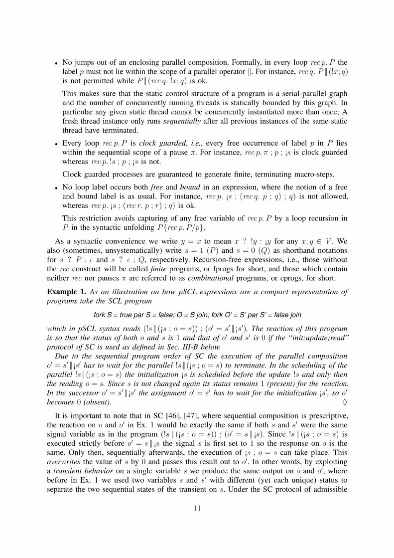
Example 1. As an illustration on how pSCL expressions are a compact representation ofprograms take the SCL program

fork S = true par S = false; O = S join; fork O’ = S’ par S’ = false join

which in pSCL syntax reads (!s || (¡s ; o = s)) ; (o′ = s′ || ¡s′). The reaction of this programis so that the status of both o and s is 1 and that of o′ and s′ is 0 if the “init;update;read”protocol of SC is used as defined in Sec. III-B below.

Due to the sequential program order of SC the execution of the parallel compositiono′ = s′ || ¡s′ has to wait for the parallel !s ||(¡s ; o = s) to terminate. In the scheduling of theparallel !s ||(¡s ; o = s) the initialization ¡s is scheduled before the update !s and only thenthe reading o = s. Since s is not changed again its status remains 1 (present) for the reaction.In the successor o′ = s′ || ¡s′ the assignment o′ = s′ has to wait for the initialization ¡s′, so o′

becomes 0 (absent). ♦

It is important to note that in SC [46], [47], where sequential composition is prescriptive,the reaction on o and o′ in Ex. 1 would be exactly the same if both s and s′ were the samesignal variable as in the program (!s || (¡s ; o = s)) ; (o′ = s || ¡s). Since !s || (¡s ; o = s) isexecuted strictly before o′ = s || ¡s the signal s is first set to 1 so the response on o is thesame. Only then, sequentially afterwards, the execution of ¡s ; o = s can take place. Thisoverwrites the value of s by 0 and passes this result out to o′. In other words, by exploitinga transient behavior on a single variable s we produce the same output on o and o′, wherebefore in Ex. 1 we used two variables s and s′ with different (yet each unique) status toseparate the two sequential states of the transient on s. Under the SC protocol of admissible

11

“init;update;read” schedules the transient on s is not observable (other than through the outputso and o′) because every concurrent observer has to postpone its reading of s until the variableis stable, i.e., until after termination of the reset ¡s in ¡s ; o = s. So, for the concurrentenvironment of (!s ||(¡s ; o = s)) ; (o′ = s || ¡s) the variable s receives the unique final status 0.In standard SMoCs, notably Esterel and Quartz it is not possible to program transients in thisway, on signals like s that are shared between concurrent threads. However, our examplesin the previous Sec. II-A show that this is useful to code schizophrenic signals in terms ofboolean variables without non-linear code expansion. Let us look at the pSCL representationof some of these examples next.

Example 2. As an illustration on how pSCL can be employed for coding specific macro-stepsof SCL programs, consider schizo-seq-scl (Fig. 1d). At the initial tick, after entering the whileloop and until the program pauses at line 10, the sequence of statements executed are s =false; o = s; pause. In pSCL this is represented by the expression ¡s ; o = s ; π. It says thats is reset (initialized to 0) then variable o is assigned the status value s0, viz. absence andfinally the behavior pauses. From the second tick onwards, always starting and ending in thepause at line 10, the macro-step behavior of schizo-seq-scl is given by the pSCL expression¡s ; !s ; ¡s ; o = s ; π, or, in SCL, the sequence of statements s = false; s = true; s = false; o =s; pause, again ignoring the test of the while loop when wrapping around. In words, firstreset s (initialize) then, in order, set (update) and reset it (initialize) again, finally copy thestatus of s0 to variable o and pause. The full program and its sequence of macro steps canbe represented by either one of the equivalent pSCL expressions

rec p. ¡s ; o = s ; π ; ¡s ; !s ; p or ¡s ; o = s ; π ; rec q. ¡s ; !s ; ¡s ; o = s ; π ; q

where the second unfolds the loop to separate the surface behavior (first macro step up to thefirst pause) from the depth behavior (second and later macro steps). ♦

Example 3. As a more complex example involving also concurrency consider schizo-conc-cured-scl (Fig. 1f). The full program is coded by the pSCL expression

P 01f := rec p. ¡s ; ((¡term ; o = s ; π ; !s ; !term) ‖ Q) ; p

where Q := rec q. π ; ¡s ; term ? ε : q. Let us extract its individual macro-steps, therebygetting rid of loops. The surface behavior of P 0

1f is obtained by unfolding the loops

¡s ; ((¡term ; o = s ; π ; !s ; !term) ‖ (π ; ¡s ; term ? ε : Q)) ; P 01f

and extracting the code up to and including the first pauses downstream through all concurrentthreads. In this case, the surface is specified by the expression ¡s ; (¡term ; o = s ; π ‖ π)which covers the initial ¡s and the surface behaviors of the two threads until they reach theirfirst pause. In this first macro-step, thus, s is reset and sequentially afterwards the first threadresets term and copies the 0 status of s to output o. The second thread behaves as π whichpauses immediately.

The depth behavior begins with the second tick in which both threads start from theirpauses, according to the pSCL expression P 1

1f := (!s ; !term || ¡s ; term ? ε : Q) ; P o1f , which

after unfolding is the same as

(!s ; !term || ¡s ; term ? ε : (π ; ¡s ; term ? ε : Q)) ;

¡s ; ((¡term ; o = s ; π ; !s ; !term) ‖ (π ; ¡s ; term ? ε : Q)) ; P 01f

12

The second tick is given by the surface of this expression which is of the form P ′ ; ¡s ; Q′

whereP ′ := !s ; !term || ¡s ; term ? ε : π and Q′ := ¡term ; o = s ; π ||π.

First, the parallel composition P ′ is scheduled and executed as follows: Under the concurrent“init;update;read” protocol, initially, s is reset (init) and then variables s and term are set(update) in this order. After this, term is tested (read) and since its status is 1 the emptystatement ε is executed, whereupon the parallel composition P ′ joins and terminates. Thus,control continues instantaneously with the ¡s statement of the expression P ′ ; ¡s ; Q′ whichresets variable s once more. Finally, the expression Q′ gets scheduled: Since the second threadof Q′ is a pause π, it completes immediately and waits for the next tick. In the first thread,term is reset again (init) and the status of s0 is copied to variable o. Then this thread reachesπ and pauses, too. As it turns out, the third macro-step is again given by the expression P 1

1f ,so that we only need two (reachable) sequential macro states to describe the Mealy automatonfor schizo-conc-cured-scl, viz. the states coded by P 0

1f and P 11f .

Note the characteristic feature of sequentially constructive behavior in this example: Thefinal observable response of P ′ ; ¡s ; Q′ at the output o is determined by the final status 0 ofs, although during the computation of P ′ both signals s and term are set present. In SC avariable can undergo transients which are not externally observable. ♦

The imperative statements of a pSCL program describe statically (possible) discrete changesof state at the level of micro-steps. Here, an execution instance of a micro-step is called anaction. The computation of a concurrent program gets described by a collection of threads(concurrent program fragments), each one performing actions independently and interactingwith each other according to some pre-established rules of admissible scheduling, specifically,the “init;update;read” protocol to be specified below. The protocol depends on a distinctionof actions happening sequentially after each other and actions happening concurrently. Thesequential order is instantiated from sequential composition P ;Q. Parallel composition P ‖ Qis the construct that provides the required thread topology for achieving concurrency. Theresulting tree-like structure of the parallel construct determines statically which actions belongto which individual static thread. At run-time, these static threads get instantiated and executed.Every one of such instantiations must have its own local control-state and, therefore, isconsidered a process. From this perspective, the configuration capturing the global state of aconcurrent program at any given moment is determined by the local control state of all itsprocesses together with a shared global memory.

As in synchronous programming, a micro-step can take place when at least one processis active, i.e., when it is able to execute an action realizing a statement other than π. Inthis manner, a micro-step produces a change in the configuration resulting from a processexecuting an action that modifies its own local control state and possibly the global memory.Thus, in the course of an instant, active processes induce micro-steps until every process eitherterminates or reaches a pause completing with this a macro-step. Then, from the resultingconfiguration, the environment can provide a fresh stimulus for continuing the computationwith a new macro-step occurring in the next instant.

In the next Sec. III-B we define the notion of a free unconstrained execution for pSCLprograms and then in Sec. III-C introduce the admissibility restriction imposed by the“init;update;read” protocol. Based on this we can then define the class of sequentiallyconstructive pSCL programs.

13

B. Operational Free Scheduling SemanticsIn our operational model, a process T is defined by its own current control-state, or state in

short, which contains: (i) information about the precise position of T in the tree structure offorked processes and (ii) control-flow references to specific parts of the code. Formally, T isgiven by a triplet 〈id, prog, next〉 where we write T.id, T.prog or T.next for referring to theindividual elements of T which are called, respectively, (thread) identifier, current-programand next-control. Concretely,• T.id is a non-empty sequence containing an alternation of natural numbers and the

symbols l, r that always starts and ends with a number. For instance, 0.l.5 and 1.r.3.l.7are identifiers but 0.r and r.1.r.2 are not. Intuitively, 1.r.3.l.7 identifies a control statereached after 7 micro-steps in the sequential execution of the left (l) child thread of afork that has been instantiated after 3 steps within the right (r) child of an outermost forkthat has sequential index 1 in the execution of the root thread of the program. We useTI = N · ({l, r} ·N)∗ to denote the set of possible thread identifiers and the meta-variableι to range over the elements of TI .

• T.prog is the pSCL expression that is currently scheduled to generate T ’s actions. Sincecurrent-programs are pSCL expressions we use the meta-variables P , Q, etc., to rangeover these.

• T.next is a list of future program fragments that can be converted into actions sequentiallyafter T.prog has terminated instantaneously. This list is extended when a sequentialcomposition is executed in T.prog. We use the meta-variable Ks to range over next-controls.

The identifier T.id separates sequential from parallel control-flow information useful forlocalizing T in the current execution and joining previously forked processes that haveterminated. The intuition is that the numbers in the identifier are associated with the sequentialsteps taken by the process. The symbols (l for left and r for right) recall the path of previousparallel forks from which the process has emerged.

To compare the sequential depth of processes we use the (partial) lexicographic order ≺on thread identifiers TI . The natural numbers are ordered in the usual way, i.e., 0 < 1 < 2 . . .while the symbols l, r are considered incomparable. Thus, for identifiers ι = d1 . . . dn andι′ = d′1 . . . d

′m we have that ι ≺ ι′ iff

• ι is a proper prefix of ι′, i.e., n < m and ∀1 ≤ j ≤ n. dj = d′j , or• ι is lexically below ι′, i.e., there is 0 ≤ i < n such that ∀1 ≤ j ≤ i we have dj = d′j anddi+1 < d′i+1.

For instance, 0.r.2 ≺ 0.r.2.l.1 and 0.r.2.l.1 ≺ 0.r.4 but 0.r.2 6≺ 0.l.2.l.1 and 0.r.2 6≺ 0.l.4because the labels l and r are incomparable. We write � for the reflexive closure of ≺, i.e.,ι � ι′ iff ι ≺ ι′ or ι = ι′.

The order (TI ,�) contains both the thread hierarchy and sequencing in program order.Sometimes we are only interested in the depth of a process in the thread hierarchy. To extractthis we define a thread projection function th(ι) ∈ {l, r}∗ which drops from ι all sequencingnumbers. For example, th(0.r.2.l.1) = r.l and th(0) = ε, where ε denotes the empty sequence.Then, the sequence th(T.id) can be interpreted as the static thread identifier of process T .In contrast, T.id ∈ TI should be thought of as a thread instance identifier. We will use thesymbol � also for the standard prefix order on static thread identifiers {l, r}∗. For example,ε � r.l � r.l.l � r.l.l.

14

Note that there is no relationship between ι ≺ ι′ and the prefix order on th(ι) and th(ι′).The sequential successor ι′, in general, can both be a descendant or an ancestor of ι in thethread hierarchy. For instance, we have 0.r.2.l.1 � 0.r.4 but th(0.r.2.l.1) = r.l is not a prefixof r = th(0.r.4). The ordering 0.r.2.l.1 � 0.r.4 expresses that the 4th action of the rightchild of the root thread happens sequentially after the l.1 successor within the 2nd action ofthe same child. This 2nd action 0.r.2.l.1 is a sequential predecessor but a descendant of the4th action in the thread hierarchy. In the other direction, 0.r.2 is a sequential predecessor of0.r.2.l.1 but r = th(0.r.2) is an ancestor of r.l = th(0.r.2.l.1).

The sequential enumeration for identifier ι is computed by an increment function inc(ι)which increases by 1 the last number of the identifier ι, e.g., inc(1.r.6) = 1.r.7.

Formally, the global memory is a boolean valuation function ρ : V → B which stores thecurrent value for each variable. The action of a process T (relative to a given memory ρ)produces a new memory ρ′ and a set of successor processes S. Thus, any action is completelyspecified by the update function ρ′ := upd(T, ρ) and the succession function S := nxt(T, ρ)according to the following Def. 1:

Definition 1. For a given x ∈ V , the update function is defined by:

upd(T, ρ)(x) :=

0 if T.prog = ¡s and x = s

1 if T.prog = !s and x = s

ρ(x) otherwise.

This says that for a given variable s ∈ V , if T performs a reset ¡s then s is changed to 0, ifT performs a set !s then s is changed to 1, otherwise, s keeps its value from the previousmemory. We define the succession nxt(T, ρ) by case analysis on T.prog and T.next:

nxt(〈ι, P, [ ]〉, ρ) := ∅ if P ≡ ε, P ≡ ¡s or P ≡ !s (1)nxt(〈ι, P,Q::Ks〉, ρ) := {〈inc(ι), Q,Ks〉} if P ≡ ε, P ≡ ¡s or P ≡ !s (2)nxt(〈ι, P ; Q,Ks〉, ρ) := {〈ι, P,Q::Ks〉} (3)

nxt(〈ι, rec p. P,Ks〉, ρ) := {〈ι, P{rec p. P/p},Ks〉} (4)

nxt(〈ι, s ? P : Q,Ks〉, ρ) :=

{{〈inc(ι), P,Ks〉} if ρ(s) = 1

{〈inc(ι), Q,Ks〉} otherwise(5)

nxt(〈ι, P ||Q,Ks〉, ρ) := {〈ι, ε,Ks〉, 〈ι.l.0, P, [ ]〉, 〈ι.r.0, Q, [ ]〉}. (6)

Let us explain the different cases in the definition of nxt one by one:• If the program T.prog is one of the atomic statements empty ε, set !s or reset ¡s and the

list of continuation processes in the next-control T.next is empty [ ], then the process(after execution) is terminated and disappears from the configuration. This is achieved bysetting the succession to be the empty set.

• If T.prog is empty one of the atomic statements and the list of continuation processes inT.next is a non-empty list Q::Ks , then we start Q in a new process with next-controlKs and a sequentially incremented index inc(ι).

• If T.prog is a sequential composition P ; Q then we start P in a new process with thesame identifier and add Q to the front of the next-control list. The identifier does not

15

increment since we do not consider the new process 〈ι, P,Q::Ks〉 a sequential successorbut only a structural replacement.

• A loop T.prog = rec p. P behaves like its unfolding P{rec p. P/p}, without modificationto the identifier and next-controls.

• Next consider a process with conditional program T.prog = s ? P : Q in memory ρ.Depending on whether the memory value for the variable s is 1 or 0 we install the P orthe Q branch, respectively, with an incremented identifier and the same next-control. Theidentifier is incremented because the branches are considered as being executed strictlyafter the conditional test, in sequential program order.

• Finally, executing a parallel program T.prog = P ‖ Q instantiates the two sub-threads Pand Q in their own process 〈ι.l.0, P, [ ]〉 and 〈ι.r.0, Q, [ ]〉, respectively, with a fresh andempty next-control but extended identifiers. The process P is the left child of the parentprocess 〈ι, P ||Q,Ks〉. Therefore, we add the suffix l.0 to the parent’s identifier, andanalogously r.0 for the right child Q. At the same time that the parent process forks itstwo children it transforms itself into a join process 〈ι, ε,Ks〉. Since ι ≺ ι.l.0 and ι ≺ ι.r.0both children have strictly larger identifiers. Since only processes with maximal identifiersare executable (see below) the join process must wait for the children to terminate beforeit can release the next-controls Ks , or terminate itself in case Ks = [ ].

Note that there is no clause for the succession of a pausing process or a process label, i.e.,nxt(〈ι, π,Ks〉, ρ) and nxt(〈ι, p,Ks〉, ρ) are undefined. This is no problem since (i) program πis never executed in a micro-step action but only by the next global clock tick (see below),and (ii) we are only interested in the behavior of closed pSCL expressions which do not haveany free process labels.

Example 4. Consider the process T0 = 〈0, ¡s ; o = s, [ ]〉 with T0.prog containing the pSCLexpression corresponding to program schizo-seq-scl (Fig. 1d) for the initial tick. Startingfrom a memory ρ0 that gives value 1 to every variable, let T0 make its first action to obtainnew memory ρ1 = upd(T0, ρ0) and a set of successors S1 = nxt(T0, ρ0) according to (3).As it is easy to see, this action does not modify the memory, i.e., ρ1 = ρ0 and results in asingleton set S1 = {T1} where T1 = 〈0, ¡s, [o = s]〉. Basically, this action has separated thetwo sequential statements of the original program. Now proceeding with T1 from ρ1, we cometo execute the reset ¡s, obtaining ρ2 and successors S2. Memory ρ2 now gives value 1 to allthe variables except for s whose value is changed to 0. Following (2), the succession is thesingleton S2 = {T2} with process T2 = 〈1, o = s, [ ]〉. Notice the increment of the identifierwhich reflects the fact that execution has passed a sequential composition operator. Now recallthat o = s stands for the conditional s ? !o : ¡o, so the value of s is tested in memory ρ2.We have ρ2(s) = 0, whence ρ3 = ρ2 and S3 = {T3} with T3 = 〈2, ¡o, [ ]〉 as described by (5).From here, the reset ¡o yields a new memory ρ4 in which the value of every variable is 1apart from o and s that have value 0. Since S4 = ∅ by (1), there are no more processes fromwhich we can continue. This completes the computation by instantaneous termination. ♦

Let us combine the update and succession functions for a single process to define themicro-steps of an arbitrary set of processes running concurrently.

Definition 2. A configuration is given by a pair (Σ, ρ), where ρ is the global memory and Σ,called the process pool, is a finite set of (closed) processes such that• all identifiers are distinct, i.e., for all T1, T2 ∈ Σ, if T1.id = T2.id then T1 = T2;• the sequential ordering of identifiers coincides with the thread hierarchy, i.e., for all

16

T1, T2 ∈ Σ, we have T1.id � T2.id iff th(T1.id) � th(T2.id) (prefix ordering);• the identifiers form a full thread tree, i.e., for each T ∈ Σ and every prefix (ancestor)t ∈ {r, l}∗ with t � th(T.id), there is a process T ′ ∈ Σ of T with th(T ′.id) = t and forany two T1, T2 ∈ Σ there is a common ancestor T ∈ Σ so that th(T.id) � th(T1.id) andth(T.id) � th(T2.id).

The micro-step execution to be defined shortly will maintain this structural invariant ofprocess pools. Note that in every process pool there is a root process Root ∈ Σ whose identifierRoot.id is a single natural number n with th(Root.id) = th(n) = ε.

We call a process T ∈ Σ pausing when T.prog = π. T is active if T.id is �-maximal(identifier order) in Σ and T is not pausing. T is waiting if is neither pausing nor active. Aconfiguration Σ is quiescent if it does not contain any active processes or, in other words, ifall the processes T ∈ Σ are waiting or pausing. Note that for any memory ρ, a configurationof the form (∅, ρ) is trivially quiescent.

From a given non-quiescent configuration (Σ, ρ) and a selection T ∈ Σ of an active process,we can let T execute its first action to produce a micro-step

(Σ, ρ)T→µs (Σ′, ρ′),

where in the free scheduling there is no constraint on T other than it being active. The resultingmemory

ρ′ := upd(T, ρ)

is computed directly from the upd function. The new process pool Σ′ is obtained by removingT from Σ and replacing it by the set of successors generated by nxt , i.e.,

Σ′ := Σ \ {T} ∪ nxt(T, ρ).

Note that in the free schedule both the next process pool Σ′ and the updated memory ρ′

only depend on the active process T that is executed and the current memory ρ. They do notdepend on the other states in Σ. Since the successor configuration is uniquely determinedby (Σ, ρ) and T , we may write (Σ′, ρ′) = T (Σ, ρ).

In a micro-sequence R the scheduler runs through a succession

R = (Σ0, ρ0)T1→µs (Σ1, ρ1)

T2→µs · · ·Tk→µs (Σk, ρk) (7)

of micro-steps obtained from the interleaving of process actions. We let �µs be the reflexiveand transitive closure of →µs. More precisely, we write

R : (Σ0, ρ0)�µs (Σk, ρk)

to express that there exists a micro-sequence R, not necessarily maximal, from configuration(Σ0, ρ0) to (Σk, ρk). We can view R as a function mapping each index 1 ≤ j ≤ k to the processR(j) = Tj executed at micro-step j and len(R) = k is the length of the micro-sequence,i.e., the number of actions executed.

A synchronous instant, or instant for short, abbreviated

R : (Σ0, ρ0) =⇒µs (Σk, ρk). (8)

is a maximal micro-sequence that reaches a final quiescent configuration (Σk, ρk).

17

({T0}, ρ0) ({T1}, ρ0) ({T20, T21, T22}, ρ0)

({T20, T31, T22}, ρ0) ({T20, T21, T32}, ρ0)

({T20, T31, T32}, ρ0)({T20, T41, T22}, ρ11) ({T20, T21, T42}, ρ12)

({T20, T41, T32}, ρ11) ({T20, T31, T42}, ρ12)

({T20, T41, T42}, ρ11)({T20, T41, T42}, ρ12)

({T20}, ρ21)

({T20, T42}, ρ21)

({T20, T32}, ρ21)

({T20, T42}, ρ22)

({T20, T522}, ρ22)

¡s

({T20, T521}, ρ22)

;

({T20}, ρ22)

!term !s

!s

term?

¡s

;

;

;

;

;

({T20, T31, T522}, ρ12)

({T20, T41, T522}, ρ11)

fork

({T20, T522}, ρ21)

¡s

!term

!term

!termterm?

term?

²

({T3}, ρ21)

;

¡s

!s

!s

term?

term?

!term

join

({T20, T41, T522}, ρ12)

({T3}, ρ22) pausing

A

B({T20, T22}, ρ21)

!term

;

pausing

({T20, T521}, ρ21)²

join

Fig. 2: The free scheduling graph of process T0 of Ex. 5.

There are two ways in which the final configuration (Σk, ρk) may be quiescent. If Σk isempty, then we say that the instant is terminated instantaneously. When (Σk, ρk) is quiescentbut not empty then the instant is pausing. All remaining processes are waiting for the clockto tick. Such a clock tick

(Σk, ρk) =⇒tick (Σ′, ρ′)

consists of replacing every pausing process 〈ι d, π,Ks〉 ∈ Σk by a new process 〈ι 0, ε,Ks〉 ∈ Σ′

preserving the sequential identifier of all ancestors but restarting the current thread at sequencenumber 0. The new memory ρ′ preserves all internal and output variables but permits theenvironment to change all input variables for the next macro-step. For the investigations in thisreport, however, we are only interested in single macro-steps generate by the surface behaviorof pSCL expressions. Therefore, we will not be concerned with clock ticks any further.

Example 5. Let (Σ0, ρ0) be a configuration where ρ0 gives value 0 to every variable and theprocess pool Σ0 = {T0} consists of the following root process:

T0 = 〈0, (!s ; !term || ¡s ; term ? ε : π) ; Q, [ ]〉.If Q = ¡s ; (¡term ; o = s ; π || π), then this is precisely the macro-step behavior schizo-conc-cured-scl (Fig. 1f) from its second tick onwards, as explained in Ex. 3. The complete

18

computation graph for the free scheduling from (Σ0, ρ0), up to activation of Q, is depicted inFig. 2. The processes are abbreviated as follows:

T0 = 〈0, (!s ; !term ‖ ¡s ; term ? ε : π) ; Q, [ ]〉 T31 = 〈0.l.0, !s, [!term]〉T1 = 〈0, !s ; !term ‖ ¡s ; term ? ε : π, [Q]〉 T32 = 〈0.r.0, ¡s, [term ? ε : π]〉T20 = 〈0, ε, [Q]〉 T41 = 〈0.l.1, !term, [ ]〉T21 = 〈0.l.0, !s ; !term, [ ]〉 T42 = 〈0.r.1, term ? ε : π, [ ]〉T22 = 〈0.r.0, ¡s ; term ? ε : π, [ ]〉 T3 = 〈1, Q, [ ]〉T521 = 〈0.r.2, ε, [ ]〉 T522 = 〈0.r.2, π, [ ]〉

Each edge in Fig. 2 is a single micro-step. For better readability we do not use the selectedprocess Ti as the label but instead the primitive operator executed in the action, i.e., asequential composition (;), set statements (!s, !term), reset (¡s), the empty program (ε), a forkor a join. The shaded regions named A and B will be explained later.

Since T0 is active it can induce the micro-step (Σ0, ρ0)→µs (Σ1, ρ0) where Σ1 = {T1}. Then,letting T1 do its action (Σ1, ρ0)→µs (Σ2, ρ0) we obtain a succession Σ2 = {T20, T21, T22} ofthree processes as a result of executing the parallel fork, the parent T20 and its two childrenT21 and T22. Observe that in Σ2 the two children are active but the parent with identifier0 is waiting, because 0 ≺ 0.l.0 and 0 ≺ 0.r.0. The parent T20 plays the role of a join inthe sense that it cannot execute any action until the two children terminate and its ownidentifier becomes maximal again. Let us suppose that first T21 and then T22 are scheduledto get (Σ2, ρ0) �µs (Σ4, ρ0) with Σ4 = {T20, T31, T32}, where T31 and T32 are both active.Here things become interesting since the chosen scheduling order will result in differentconfigurations. For if (Σ4, ρ0)�µs (Σ6, ρ11) results from scheduling T32 followed by T31, thenfirst the reset ¡s is performed and thereafter the set !s, so that ρ11(s) = 1. On the otherhand, if first T31 is picked and then T32 does its initial action, then (Σ4, ρ0) �µs (Σ6, ρ12)with ρ12(s) = 0. Although the resulting process pool Σ6 = {T20, T41, T42} is the same in bothconfigurations, the global memory is not. Continuing the schedule from configuration (Σ6, ρ11)we see that there is a race between the reading of variable term by T42 and the write toterm by T41. If we first execute T41, then the conditional T42 will activate its ‘then’-branch ε.Therefore, we eventually reach the configuration (Σ9, ρ21) with Σ9 = {T3} and the memorysatisfies ρ21(s) = ρ21(term) = 1. Now program Q is active in T3 and instantaneously takesover control for the rest of the micro-sequence computation. On the other hand, if in (Σ6, ρ11)the process T42 first gets to test the value of term , which is 0, before T41 sets it to 1, then the

‘else’-branch is selected and we end up in the configuration (Σ8, ρ21) where Σ8 = {T20, T522}.This configuration is quiescent as it contains no active processes. The program Q is waiting inthe join process T20 which has a strictly smaller identifier than process T522 which is pausing.No progress can be made until the next clock tick makes T522 disappear from the configuration,thereby activating T20. Note that the conflict between T41 and T42 in (Σ6, ρ11) results in anon-determinism of control, viz. either executing Q in the same instant or not. On the otherhand, the race between T31 and T32 in (Σ4, ρ0) generates nondeterminacy of the final memoryin that we can either pause in ({T20, T522}, ρ22) of region A or in ({T20, T522}, ρ21) of regionB which have the same process pool but different variable assignments. ♦

Not surprisingly, as demonstrated in Ex. 5 the selection strategy applied in the free schedulingof a program determines the final memory content at the end of a macro-step. Such non-determinacy can be eliminated by restricting the free scheduling to so-called admissibleschedules that are natural for the programmer and at the same time reliably implemented onthe chosen run-time platform by a trusted compiler. A canonical such notion of admissibility

19

is obtained from enforcing the “init;update;read” protocol which decrees that all concurrentinitializations ¡s must take place before any concurrent update !s which in turn must bothbe scheduled before any concurrent read, i.e., any conditional test s ? P : Q on s. This willeliminate the scheduling regions called A and B in Fig. 2 and enforce determinacy.

The “init;update;read” protocol can be refined by limiting the number of initializations thatare permitted during a single macro-step on any variable. The most liberal stand, allowingan arbitrary number of sequential “init;update;read” cycles leads to the notion of sequentialconstructiveness, or ∆∗-constructiveness, which is introduced in the next section.

C. ∆∗ ConstructivenessAs was illustrated in Ex. 3, a (well-formed) pSCL program can be separated into its

individual macro-step reactions, each of which is expressible without loops. Since the mainresults in this report concern the scheduling of actions inside a single finite macro-step, withoutloss of generality, henceforth we will consider pSCL programs without loops, referred to asfinite programs or fprogs for short. In addition, since each of these fprogs only describes asingle instant, we are only interested in its surface behavior. The depth behavior belongs tothe next synchronous instant and is captured by a different (continuation) fprog.

The “init;update;read” protocol of SC imposes a natural execution order on the accesses toa variable during a macro-step. In the general setting [46], [47] this depends on classifying thewrite accesses into so-called absolute writes for initialization, and so-called relative writes toperform the update. This classification is not fixed but leaves room for different interpretationsin specific compilers, specific application domains or even specific programs. The key criterionis that the order in which any two relative writes are executed must be immaterial, i.e., resultin the same (or at least observably equivalent) memory states, so that all concurrent relativewrites may be scheduled freely without jeopardizing determinacy. A typical class of relativewrites is obtained by assignments of the form x = f(x, ex), where f is a commutative andassociative binary function and ex an arbitrary expression which does not depend on x. Suchfunctions f are known as combination functions in SMoCs (see, e.g. [10], [4], [39]) or asresolution functions in VHDL (see, e.g. [25]). Once the relative writes have been determined,all other write accesses are classified as absolute writes in SC.

The “init;update;read” protocol also applies to pure signals in SMoCs. The signal emissionemit x in pure Esterel, for instance, is an update on boolean values with logical disjunction|| acting as the combination function, i.e., the assignment x = x || true. This is equivalentto the constant assignment x = true which corresponds to the set operation !x in pSCL. Anywrite that sets a signal to absent is an absolute write in SC terminology. Such resets x = false,which are implicit in Esterel, now become first class write accesses ¡s in pSCL under thecontrol of the programmer. The “init;update;read” protocol (implemented by the compiler)makes sure the resets are scheduled before any set. Since reads are scheduled after any write,the variables’ boolean values perfectly reflect the synchronous semantics of signals: A signalvariable x is read to be present (value true) by the concurrent environment if x is emitted bythe system, and x is read as absent (value false) if x is initialized and never emitted.

To ensure determinacy the SC model of computation does not permit two concurrent writeshappening within the same macro-step unless they are confluent. For relative writes this isguaranteed by definition. Absolute writes also may be confluent with each other. For instanceconsider the pSCL expression P ‖ ((!s ‖ !s) ; Q). Trivially, the two concurrent resets on signal

20

s can be executed in any order without affecting its concurrent context P or its sequentialcontext Q. Similarly, once a signal s has been emitted, and thus its value is set to 1, lateremissions may safely happen after any read of s, provided there has not been any reset inbetween. For instance, in !s ; (s ? !s ; P1 : P2 ‖ !s) ; Q the order of execution between thetest s? and the concurrent !s does not influence the result. Similarly, the emission !s in the‘then’-branch of the conditional takes place after the read, which is innocuous as the value ofs has been set already. Generally speaking, the strict “init;update;read” ordering in the settingof SC is applied only to variable accesses that are both concurrent and non-confluent. Thefollowing Defs. 3 and 4 formalise this idea which is instrumental to understand synchronoussignals in terms of shared memory variables.

Definition 3 (Independence of Processes). Two processes T1, T2 are called conflicting in aconfiguration (Σ, ρ) if(i) T1, T2 ∈ Σ are both active in Σ and

(ii) T1(T2(Σ, ρ)) 6= T2(T1(Σ, ρ))

Processes T1, T2 are confluent with each other, or independent in (Σ, ρ), written T1 ∼(Σ,ρ) T2,if there is no micro-sequence (Σ, ρ) �µs (Σ′, ρ′) such that T1 and T2 are conflicting in(Σ′, ρ′).

Example 6. As an illustration consider once more Example 5. Processes T31 and T32 areconflicting in configuration (Σ4, ρ0) = ({T20, T31, T32}, ρ0) because, as we have seen, both areactive in this configuration and, moreover, different execution orders lead to different results.Since the action of T31 is !s (update) and the action of T32 is the reset ¡s (init), the schedulingprotocol gives precedence to T32. Similarly, T41 and T42 are in conflict in configuration(Σ6, ρ12) with Σ6 = {T20, T41, T42} as can be seen from Fig. 2. For their part, processes T21

and T22 are independent or confluent in (Σ2, ρ0) with Σ2 = {T20, T21, T22}. This is so becausein every micro-sequence (Σ2, ρ0)�µs (Σ′, ρ′) the only configuration in which both T21 andT22 are active is precisely (Σ2, ρ0). Furthermore, as can be seen from Fig. 2, the order ofexecution is unimportant in this case, namely T21(T22(Σ2, ρ0)) = T21(T22(Σ2, ρ0)) = (Σ4, ρ0),where Σ4 = {T20, T31, T32}. Note that since the initial action of both T21 and T22 is thebreaking up of the sequential composition, and thus not variable accesses, their ordering isunconstrained by the “init;update;read” scheduling protocol. ♦

For a micro-sequence or synchronous instant R a process instance of R is given by apair ni = (T, i) with 1 ≤ i ≤ len(R) where T = R(i). This indexing internalizes thehappens-before relation directly on the process actions and permits us to view R as a linearlyordered set of actions.

Example 7. Take the micro-sequence R1 : (Σ0, ρ0)�µs (Σ10, ρ10) of Ex. 5 with len(R1) = 10and R1 = T0, T1, T21, T22, T32, T31, T41, T42, T521, T20. It maps the micro-step indices 1 ≤i ≤ 10 to actions R1(i) defined by the order of execution, i.e., R1(1) = T0, R1(2) = T1,R1(3) = T21, and so on and so forth. Hence, n1 = (T0, 1), n2 = (T1, 2), n3 = (T21, 3), n4 =(T22, 4), . . . , n10 = (T20, 10) are all the process instances of R1. Note the sequence ofprocess identifiers R1(i).id in this sequence is 0, 0, 0.l.0, 0.r.0, 0.r.0, 0.l.0, 0.l.1, 0.r.1, 0.r.2, 0.So, different process instances do not necessarily have different identifiers. However, theactions consisting of atomic program statements in the sequence R1, those are ¡s, !s, !term,?term and ε, all have distinct identifiers. ♦

21

Definition 4 (Concurrency, Confluence and Scheduling Order). Consider a micro-sequence

R : (Σ0, ρ0)�µs (Σk, ρk)

and two of its process instances ni1 = (R(i1), i1) and ni2 = (R(i2), i2). We define thefollowing relations between ni1 and ni2:

1) ni1 and ni2 are concurrent, ni1 | ni2, if R(i1).id 6� R(i2).id and R(i2).id 6� R(i1).id.2) ni1 precedes ni2, abbreviated ni1 →pre ni2, if ni1 | ni2 and either:

(i) ni1 performs a reset ¡s or set !s on a variable s that is read (tested) by ni2, or(ii) ni1 performs a reset ¡s on a variable s on which ni2 performs a set !s.

3) ni1 and ni2 are confluent or independent in R, written ni1 ∼R ni2, if R(i1) ∼(Σj ,ρj)

R(i2), where j = min(i1, i2)− 1.4) ni1 happens before ni2 in R, indicated ni1 →R ni2, if i1 < i2.

Example 8. From the micro–sequence R1 of Ex. 7, we have the following. Clearly, n3 →R1 n5

since R1(3) = T21 is scheduled (happens) before R1(5) = T32. This does not imply thatT21 is a sequential predecessor of T32 in program order. In fact, we have n2 | n5 preciselybecause the identifier T21.id = 0.l.0 and T32.id = 0.r.0 are �-incomparable. Note that theconcurrency relation is static in the sense that it indicates that the processes could (but mustnot) be both active in some configuration. In the same order of ideas, n2 and n4 are notconcurrent since R1(2) = T1.id = 0 � 0.r.0 = T22.id = R1(4) which indicates that T1 is asequential predecessor of T22. Observe that non-concurrent (sequential) processes, such as T1

and T22, when appearing in the same sequence, always do so according to the �-order oftheir identifiers, i.e., n2 →R1 n4. ♦

Comparing Def. 4 with the corresponding definition in the general setting of SC (Def. 4,Def. 8 and Def. 9 in [47]) two remarks are in order:

• First, as seen in Def. 4(1) concurrency of processes can now be defined simply bycomparing the process identifiers as these contain sequencing information. Whenever twoidentifiers T1.id and T2.id are �-incomparable the processes T1 and T2 are concurrent.This implies that they belong to concurrent static threads, i.e., th(T1.id) and th(T2.id)are incomparable under the prefix ordering in {l, r}∗. The converse does not hold as thefollowing example shows:Example 9. Consider the expression ((!s ; P1) ‖ P2) ; (Q1 ‖ Q2). The execution of P1

leads to a process with identifier T1.id = 0.l.1 as the second micro-state in the left childthread of root. The later execution of Q2 starts up with the identifier T2.id = d.r.0 asthe first micro-state of the right child thread which is instantiated from the fork Q1 ‖ Q2

that appeared with some sequential index d ≥ 1 after the join of (!s ; P1) ‖ P2. Now,obviously th(T1.id) = l and th(T2.id) = r which are incomparable. However, T1 and T2

are not concurrent since T2 is a sequential successor of T1. This is witnessed under the≺-order which gives T1.id = 0.l.1 ≺ d.r.0 = T2.id. ♦In [47] the “processes” are statement nodes of a sequential concurrent control flow graph(SCG) together with a scheduling status. They do not contain dynamic sequence identifiers.Instead, concurrency is derived by checking that both nodes have been spawned fromthe same instance of their least common ancestor fork in the static thread graph (cf.Def. 4 in [47]). Since this definition needs the full context of the micro-sequence Rthe concurrency relation is written ni1 |R ni2 in [47] rather than ni1 | ni2 as here. Thefact that concurrency is derived from the sequentiality relation �, rather than being a

22

primitive concept, motivates the choice of the term “sequentially” constructive for ournew model of synchronous of computation.

• The second remark concerns clause (2) of Def. 4 which captures the essence of the“init;update;read” protocol. In the general formulation of SC we must also impose aprecedence relation between any two concurrent absolute writes since these are notnecessarily confluent with each other. This is not needed here for pSCL in which theonly absolute write is the reset ¡s. It suffices to order initializations before updates, seeDef. 4(2)(i) and writes before reads, see Def. 4(2)(ii). Another, though minor, differenceis that here the precedence ordering is defined independently from whether the processinstances are confluent or not. Precedence according to the formulation in [47] notonly requires concurrency like our Def. 4 does, but also non-confluence. Here, we findit more perspicuous to leave confluence aside and take care of it in the definition of∆∗-admissibility Def. 5 below, which coincides with the notion of sequential admissibility(cf. Def. 10 in [47]).

Definition 5 (∆∗-Admissibility). A micro-sequence R is ∆∗-admissible iff for all processinstances in R, with 1 ≤ i1, i2 ≤ len(R) and n1,2 = (R(i1,2), i1,2), the following ∆∗ schedulingcondition is satisfied: Whenever ni1 precedes ni2 according to protocol order, then ni1 happensbefore ni2 or both are confluent in R. Formally, if ni1 →pre ni2, then ni1 →R ni2 orni1 ∼R ni2.

The following definition coincides with the notion of sequential constructiveness (cf. [46],[47]) for the special case of fprogs and only refers to the surface behavior:

Definition 6 (∆∗-Constructiveness). A fprog P is ∆∗-constructive (SC) iff for all initialconfigurations (Σ0, ρ0), where Σ0 = {〈0, P, [ ]〉},(i) there exists a ∆∗-admissible synchronous instant (Σ0, ρ0) =⇒µs (Σk, ρk) and

(ii) every ∆∗-admissible synchronous instant leads to the same configuration (Σk, ρk).

Note that in Def. 6 the final configurations (Σk, ρk) always have a process pool Σk inwhich all remaining processes are pausing. This is so because any synchronous instant, bydefinition, reaches a quiescent configuration without active processes. Hence, there may be atmost pausing processes left over. However, for fprogs without pause construct, the uniquereachable quiescent process pool is empty Σk = ∅.

Example 10. Consider P := s ? (x = 0 (!y)) : (y = 0 (!x)). This program does notcontain any parallel operator. Thus, for arbitrary initial memories, P admits of exactlyone schedule. Further, since P does not generate any concurrent variable accesses, everyschedule is ∆∗-admissible. Hence, P is ∆∗-constructive. The binary-branching conditionalcan be coded equivalently in terms of a parallel composition of one-sided conditionalsP ′ := (s = 1 (x = 0 (!y))) ||(s = 0 (y = 0 (!x))). This now contains a parallel compositionoperator. Still, because the concurrent accesses x = 0 and !x to x (and analogously to y)are guarded by the value of s and mutually exclusive, no single execution actually containsconcurrent accesses to x (or y). Therefore, again every schedule is ∆∗-admissible. In fact,one can show that every micro-step of P ′ can be simulated by zero or one micro-step of P sothat the sequence of memories produced are the same for both programs. This implies that P ′

is ∆∗-constructive and equivalent to P .Note that the final response of each program P and P ′ depends on the initial condition.

For ρ0(s) = ρ0(x) = ρ0(y) = 0 the final memory ρk has ρk(s) = ρk(y) = 0 and ρk(x) = 1,

23

whereas for initial memory ρ′0(s) = 1 and ρ′0(x) = ρ′0(y) = 0 we get ρ′k(s) = ρ′k(x) = 0 andρ′k(y) = 1. ♦

∆∗-constructiveness captures responsiveness and determinacy under non-determinism arisingfrom thread scheduling. As highlighted in Ex. 10 this does not preclude that a program producesdifferent final responses for different initial memories. In fact, the response usually dependson the initial value of variables that act as input variables. This form of non-determinism isnormally not considered harmful since the value of input variables are assumed to be safelycontrolled and synchronized by the “environment” of a program. However, it may sometimesbe necessary to enforce determinism for output variables. The final value of a variable thatacts as an output is usually supposed to be uniquely (causally) determined by the program. Itshould not depend on the output variables’ initial memory state if this initial memory is notunder control of the program but the compiler, operating or run-time system. For instance, instandard Java/C programming one might be tempted to assume all memory is initialized tobinary 0, at run-time, before the program starts. Obviously, in view of modern security attacksit would be haphazardous to rely on any default initializations outside of the applicationprogram. Therefore, it may be useful to strengthen the notion of constructiveness to includesome form of robustness under external non-determinism also regarding initial memory andexternal input.

A general form of constructiveness that allows us to make assumptions on the run-timeguaranteeing certain default initializations and at the same time expressing robustness underthe remaining environmental uncertainty can be obtained by using partial equivalence relationson memories. A partial equivalence relation is a subset Π of disjoint (non-empty) sets π ofmemories ρ. Two memories ρ1 and ρ2 are equivalent with respect to Π, written ρ1 ≡Π ρ2 ifthere exists an equivalence cluster π ∈ Π such that ρ1 ∈ π and ρ2 ∈ π. The relation ≡Π isobviously symmetric by definition. It is transitive because the equivalence clusters in Π areall disjoint. On the other hand, ≡Π is not reflexive in general, since ρ 6≡Π ρ iff there exists nocluster π ∈ Π such that ρ ∈ π. Such ρ are sometimes referred to as partial elements, hencethe name ‘partial’ equivalence relation. We now use such partial equivalence relations to refinethe definition of ∆∗-constructiveness. Partial memories are used to express don’t cares, i.e.,initial memories that are guaranteed never to occur at run-time and the clusters express anyremaining uncontrollable non-determinism about the initial conditions.

Definition 7 (∆Π∗ -Constructiveness). Let Π be a partial equivalence relation on memories, i.e.,

on functions V → B. Then, a fprog P is ∆Π∗ -constructive, or ∆∗-constructive with respect to

Π, iff for all initial configurations (Σ0, ρ0), where Σ0 = {〈0, P, [ ]〉} and ρ0 ≡Π ρ0,(i) there exists a ∆∗-admissible synchronous instant (Σ0, ρ0) =⇒µs (Σk, ρk) and

(ii) every ∆∗-admissible synchronous instant from every initial configuration (Σ0, ρ′0) such

that ρ′0 ≡Π ρ0 leads to the same final configuration (Σk, ρk).

Generally, the more partial elements we have in Π the fewer initial memories we includein the constructiveness requirement of Def. 7, and the larger the clusters become the morerobustness we get. Obviously, ∆∗-constructiveness according to Def. 6 is the same as ∆Id

∗ -constructiveness, according to Def. 7, with respect to the identity relation Id as the partialequivalence. Note that for the identity relation Id we have ρ0 ≡Id ρ′0 iff ρ0 = ρ′0, i.e., thereare no partial elements and all clusters are singletons. For any subset M ⊆ V → B ofmemories we can consider the partial identity Id(M) = {{ρ} | ρ ∈ X}. For this relation,then, constructiveness ∆

Id(M)∗ restricts scheduling independence of Def. 6 to initial memories

24

in M . In this way, default initializations can be accommodated for a weakened notion ofconstructiveness. For instance, pure signals in Esterel have a default initialization to status0. On the other hand, a stronger form of constructiveness would be needed to accommodateinitial jitter on output variables. For any set of (output) variables O ⊆ V let Out(O) be the(total) equivalence relation such that ρ1 ≡Out(O) ρ2 iff ρ1(x) = ρ2(x) for all x ∈ V \O. Thissays that ρ1 and ρ2 may differ in their value on variables O but are identical otherwise. Forthis relation, then, constructiveness ∆

Out(O)∗ requires that the final response of a program must

be deterministic under arbitrary ∆∗-admissible scheduling and arbitrary initial values on the(output) variables O, for any fixed initial memory on the other variables V \O.

Example 11. Let us revisit Ex. 10 with program P := s ? (x = 0 (!y)) : (y = 0 (!x)) fromthe refined point of view. It is ∆∗-constructive under Def. 6 but not ∆

Out(O)∗ -constructive

if we consider O = {x, y} as the set of output variables which are meant to be uniquelydetermined by the execution of P regardless their initial value. Indeed, if the initial conditionis ρ0(s) = ρ0(x) = ρ0(y) = 0 the final memory ρk has ρk(s) = ρk(y) = 0 and ρk(x) = 1,whereas for initial memory ρ′0(s) = ρ′0(x) = 0 and ρ′0(y) = 1 we get ρ′k(s) = ρ′k(x) = 0and ρ′k(y) = 1. Hence, the final value of output x depends on the initial value of output y.Since ρ0 ≡Out(O) ρ0 and ρ0 ≡Out(O) ρ

′0 the execution of P violates condition (ii) of Def. 7 for

Π = Out(O). ♦

Observe that just like partial equivalences can be used to parameterise ∆∗-constructivenesson the initial memories, expressing a form of controllability, we can use partial equivalencesto parameterise ∆∗-constructiveness with a notion of observability Π for the final memory.Specifically, the partial elements ρk 6≡Π ρk of Π would be final memories that must neverbe obtained in any ∆∗-admissible execution, and the clustering ρk ≡Π ρ′k would express thattwo possible outcomes ρk and ρ′k count as identical, as their difference cannot be externallyobserved. An example would be fully external side-effects such as those caused by a printfstatement in C. We leave the exploration of such general notions of constructiveness to futurework. In this report we will consider only the following cases of ∆Π

∗ :• Π = Id({ρ0}) for initial memory ρ0(x) = 0 that sets all x ∈ V to 0. This is the

∆1-analysis and weak Berry-constructiveness in Sec. VI;• Π = Out(O) where O are all the variables that statically occur with write accesses in a

given program. This is the ∆0-analysis and strong Berry-constructiveness in Sec. IV-D.

IV. ∆0-CONSTRUCTIVENESS: AN ABSTRACTION FOR ∆∗-ANALYSIS

In earlier work [46] we have presented a simple static criterion for the analysis of SC-constructiveness, called ASC-schedulability. It is based on static orderings →seq and →wir onprogram statements. The former describes sequential program order and the latter staticallyover-approximates the constraints imposed by the “init;update;read” protocol, viz. →pre in thesense of Def. 4. It was shown that if the static ordering induced by →wir and →seq does notcontain any cycles with →wir edges, then the program is SC-constructive [46].

Example 12. Consider the expression P || Q where P is x ? ε : !y and Q is the fprogy ? ε : !x. The left component P sets y to 1 if x is 0 and the right sub-expression Q sets x to1 if y is 0. This is not ASC schedulable, because there is a static dependency cycle “P -read-x→seq P -write-y →pre Q-read-y →seq Q-write-x →pre P -read-x” which includes →pre edges.Indeed, if both variables x, y are initially 0, the response of P ||Q is non-determinate (under∆∗-admissible scheduling). If P is first executed to termination and then Q, we get the

25

final memory x = 0, y = 1; otherwise, if we first execute Q and then P the result will bex = 1, y = 0. Hence, P ||Q is not ∆∗-constructive. ♦

Since the ASC test is purely static it cannot deal with data dependencies. This unnecessarilyrejects programs as non-constructive although the causality cycles involving →wir are notexecutable in the run-time control flow.

Example 13. Take the fprogs P and Q as in Ex. 12. Modify their parallel composition to runconcurrently with a process that sets x to 1, i.e., P ||Q || !x. Now, by the SC rules the set !x hasto be executed before the test x? in P , which means that P does not write !y at all but behaveslike ε. As a consequence, for any given initial memory ρ0, all ∆∗-admissible executions ofP ||Q || !x produce the same determinate response, viz. where x = 1 and y = ρ0(y) is theinitial value. The fprog is ∆∗-constructive. Obviously, it is still not ASC-schedulable as definedin [46] since the static causality cycle4 involving →wir still exists. ♦

We now introduce ∆0 as an approximation to ∆∗-constructiveness on finite pSCL programswhich does account for data dependencies. It can deal with the difference of a variable retainingits original initial value from the initial memory (pristine), being initialized to 0 and then eitherremaining 0 (signal absence) or being set to 1 (signal presence). This includes monotonicvalue changes from 0 to 1 but is restricted to a single “init;update;read” cycle within a logicaltick rather than arbitrarily many as would be permitted by ∆∗-constructiveness. It is thusmore restricted than ∆∗ and essentially corresponds to Berry’s notion of constructiveness inEsterel, yet is able to deal with explicit initialisations which requires the ability to cope withprescriptive sequencing.

A. Semantic Domain I(D,P) of Signal Statuses.The ∆0 constructiveness analysis takes place in an abstract domain of information values

which describe the sequential and concurrent interaction of signals. Instead of distinguishingjust two signal statuses “absent” and “present” as in traditional SMoC, we consider thesequential behavior of a variable (during each instant) as taking place in a linearly ordered4-valued domain D := {⊥ ≤ 0 ≤ 1 ≤ >}. The linear ordering ≤ captures a trajectory througha single instance of the “init;update;read” protocol. Every declared variable starts off initiallyin status ⊥ (pristine, fixed-but-unknown). It can later be reset (i.e., initialised) to 0 and then,possibly, set (i.e., updated) to 1. On the other hand, changes from status 1 back to 0 are notpermitted. Any attempt to reset a variable sequentially after it has been set results in the value>, denoting a ∆0 model crash. The status x> indicates that more than one “init;update;read”cycle is necessary to analyze the final response of x. If this is intended, then an analysis for∆2 or above may resolve the case. Clearly, ≤ induces a lattice structure on D with minimalelement ⊥, maximal element > and the join (max) and meet (min) operations obtained in theobvious fashion.

Observe the difference between the variable values B = {0, 1}, which appear at “run-time”as defined in the operational semantics (Sec. III-B), and the variable statuses D, which are thebasis of constructiveness analysis. The latter lifts our description to a higher level in whichthe semantics of variables is enriched to reflect the fact that they are controlled by an implicitsynchronization protocol. It is the enriched semantic domain D that turns a variable into a

4In the technical report [47][Def. 13] we have relaxed the notion of ASC-schedulability to permit more informed staticapproximations of the precedence relation →pre . According to that relaxed notion the write-read dependency edge “Q-write-x→pre P -read-x” can be dropped, so the static cycle is broken.

26

(w,u)

(¹,∨)

Kleene‘s ternary domain (Esterel)

crispvalues extension for

initialisationand crash

[⊥,⊥]

[1, 1]

[0, 0]

[>,>]

[⊥, 0][⊥, 1]

I(D)

[⊥,>][0,>]

[0, 1]

[1,>]

Fig. 3: Interval Domain I(D) for Approximating Signal Statuses.

synchronized signal. We now go one step further in the abstraction. In the ∆0 analysis weoperate on predictions of variable statuses. Possible statuses of variables are approximatedby closed intervals I(D) := {[a, b] | a, b ∈ D, a ≤ b} over D. An interval [a, b] ∈ I(D) inthis 10-valued domain corresponds to the set of statuses set([a, b]) = {x | a ≤ x ≤ b} ⊆ D.Intervals [a, b] such that a < b denote uncertain information, i.e., a potential non-determinateresponse. Such a general interval represents an approximation to the final (stable) state of avariable from its two ends, the lower bound a and the upper bound b. An interval status [a, b]associated with a variable x ∈ V can thus be read as follows: “the executions of the statementsso far ensure that x has currently status a, yet it cannot be excluded that some statementsmight be executed which could increase the status of x up to b”. In this vein, the intervals[a, a] correspond to crisp, statuses which are naturally identified with the values ⊥ = [⊥,⊥],0 = [0, 0], 1 = [1, 1] and > = [>,>] of D, respectively, i.e., D ⊂ I(D). A variable s ∈ Vwith status γ ∈ I(D) is denoted by sγ .

Example 14. Assume that the status of x is not decided yet, say, it is x[⊥,>]. Then, computingthe reaction of fprog P = ¡s ; x ? !s : ε, the interval for s will be [0, 1]. The status s[0,1] forvariable s indicates that a reset ¡s must definitively be executed. Also, there is at least one set!s that can potentially be executed, but is not guaranteed, which is why the status of s rangesbetween 0 and 1. On the other hand, the response of P on variable x returns the status x⊥

reflecting the fact that x is guaranteed not to be accessed by P , therefore retaining its initialpristine value. ♦

On the status domain I(D) we can define two natural orderings:

• The point-wise ordering [a1, b1] � [a2, b2] iff a1 ≤ a2 and b1 ≤ b2, and• the (inverse) inclusion ordering [a1, b1] v [a2, b2] iff set([a2, b2]) ⊆ set([a1, b1]),

which endow I(D) with a full lattice structure for � and a lower semi-lattice structure forv. The point-wise lattice 〈I(D),�〉 has minimum element [⊥,⊥] and the minimum for theinclusion semi-lattice 〈I(D),v〉 is [⊥,>]. The element [>,>] is a maximal element for bothorderings but it is the maximum only for �. For v all singleton intervals [a, a] are maximal.

27

Join ∨ and meet ∧ for the �-lattice are obtained in the point-wise manner:

[a1, b1] ∨ [a2, b2] = [max(a1, a2),max(b1, b2)]

[a1, b1] ∧ [a2, b2] = [min(a1, a2),min(b1, b2)].

In the inclusion v-lattice the meet u is

[a1, b1] u [a2, b2] = [min(a1, a2),max(b1, b2)].

The semi-lattice 〈I(D),v〉 does not possess joins, but it is consistent complete, i.e., wheneverin a nonempty subset ∅ 6= X ⊆ D any two elements x1, x2 ∈ X have an upper bound y ∈ D,i.e., x1 v y and x2 v y, then there exists the least upper bound tX = u{y | ∀x ∈ X. x v y}.This will give us least fixed points.

Fig. 3 illustrates the two-dimensional lattice structure of I(D). The vertical direction(upwards, green arrows) corresponds to � and captures the sequential dimension of thestatuses. The horizontal direction (right-to-left, blue arrows) is the inclusion ordering v andexpresses the degree of precision of the approximation. The most precise status description isgiven by the crisp values on the left side, which are v-maximal and order-isomorphic to theembedded domain D. The least precise information value is the interval [⊥,>] on the right.

Observe that well-known ternary domain of Kleene for the fixed-point analysis of PureEsterel [9], [37] or cyclic boolean circuits [30], [32] is captured, as indicated in Fig. 3, by theinner part with values [0, 0] (“present”), [1, 1] (“absent”) and [0, 1] (“undefined”). In ternaryanalysis all signal variables are implicitly assumed initialized, hence no need for ⊥. Moreover,since there is no reset operator and thus programs cannot fail the monotonic single-changerequirement, there is no need for > either in the standard SMoC. This ternary fragment ofI(D) corresponds to three-valued Kleene logic with ∨ disjunction and ∧ logical conjunction.Fig. 3 visualizes clearly how the 10-valued domain I(D) offers an extended playground torepresent the logic of explicit initialization. The following Ex. 15 illustrates how we can usethe domain I(D) in the fixed point analysis to navigate in both dimensions � and v fordetermining the instantaneous response of a fprog.

Example 15. An initial crisp s[0,0] generated by ¡s can develop sequentially into the statuss[1,1] if a set operation must be executed on the variable afterwards, i.e., as in ¡s ; !s. However,s[0,0] may also sequentially transform into s[0,1] by a potential set operation, which is guardedby an undecided conditional and thus not yet known to be executed as in ¡s ; x ? !s : ε(cf. Ex. 14). Moreover, if this potential set operation on s is sequentially followed by a potentialreset, i.e., ¡s ; x ? !s : ε ; y ? ¡s : ε, then s[0,1] increases further in �-order and ends up ins[0,>]. All these calculated predictions for the status of s are made without any informationon the variables x and y, i.e., assuming both have status [⊥,>].

In the course of the analysis of the fprog’s context, we might eventually obtain a moreprecise description of y and as a consequence, also a more precise status for s. Let us supposewe could pin down the possible status of y to y[0,0], which lies to the left of y[⊥,>] in thediagram of Fig. 3, because [0, 0] w [⊥,>]. This updated status for y makes the reset ¡s in¡s ; x ? !s : ε ; y ? ¡s : ε un-executable. Thus, the model crash s> is no longer possible andthe information status of s can be improved, too, viz. to s[0,1] w s[0,>]. Finally, if also x isreceives a crisp value, say x[1,1] w x[⊥,>], then the status of s further narrows to the crisps[1,1] w s[0,1]. ♦

It is important to observe that the information domain I(D) does not allow us to expressarbitrary subsets of statuses. For instance, there is no representation of the constraint that a

28

variable’s status is either 0 or > but not ⊥ or 1, i.e., an abstract value for the set {0,>}. Suchgeneral subsets of D do not have the upper and lower structure necessary for our analysis. Inparticular, note that there is a difference between saying that a variable’s status lies in theinterval [0, 1] and saying its status is an element of the set {0, 1}, i.e., that its status is either0 or 1. The latter would justify a binary case analysis on the fixed but unknown status whilethe former does not. Indeed, using the interval [0, 1] we do not permit the status to be fixed aseither 0 or 1 but only as an abstract “range”. This is captures the constructive interpretationof Esterel-style causality analysis and is explained in more detail with the following Ex. 16.

Example 16. Take the fprog P = ¡s ; x ? !s : ε ; x ? ¡s : ε which is like in Ex. 15 but nowboth variables x and y are identified. The fact that the status of input x is known to lie in theset {0, 1} may be expressed in two ways: We can say (a) the status is x[0,0] or x[1,1] or (b)the status is x[0,1].

In case (a) we could argue that the final response of s in P must be [0, 0] or [>,>]:• if x has status [0, 0] then both ‘else’-branches are executed and P behaves like ¡s ; ε ; ε.

Therefore, s receives status [0, 0];• if x has status [1, 1], then both ‘then’-branches are taken and P is equivalent to ¡s ; !s ; ¡s.

Since here s undergoes a second reset its final status is [>,>].This case analysis performs two independent symbolic simulations in which the status of x isassumed to have a fixed but unknown stable value.

The second option (b) represents the status of x by the single interval [0, 1] which is amore conservative approximation. Since each conditional test in P sees the value of x asunknown in the range [0, 1] they may independently reach different decisions. This generatestwo further options, viz. that P behaves like ¡s ; !s ; ε or ¡s ; ε ; ¡s. In the former scenario thefinal status of s is [1, 1] a value that is excluded in case (a). In case (b) we do not make theassumption that the two conditional tests of x read the same value if this value is undefined.This is the conservative standpoint for Berry’s notion of constructivity where we never assumea signal is stable until we also have its value. E.g., if signal x switches from 0 to 1 in theenvironment and this change gets delayed from the point of view of the second test, then thesecond reading x ? ¡s : ε of x in P may still see x at 0 while the first reading x ? !s : εalready sees the new value 1.

Notice that symbolic simulation under scheme (b) is exponentially more efficient comparedto scheme (a) since for n unknown input variables we only need one evaluation pass withevery variable initialized to [0, 1] or [⊥,>]. Under scheme (a), if there are n input variableswe need to perform 2n different evaluations if each is stable in {0, 1} or even 4n under fulluncertainty {⊥, 0, 1,>}. ♦

In our analysis it would be possible to use the pristine status ⊥ as a constructive way tocode a fixed unknown rather than an undecided value. The status x⊥ represents a variable xwhose value is static and uniquely determined by the memory at the beginning of the macrotick. Every time where we evaluate a conditional on a variable that has crisp status ⊥ we couldsafely try both branches and combine the responses that we get from both branches. However,just like the external non-determinism discussed in Ex. 16, this creates an exponential blow-upof the complexity of the symbolic evaluation. Therefore, we will not adopt this interpretation.Instead we treat ⊥ as an undecided value and block the evaluation of conditionals.

There is one logical refinement to the domain I(D) that we need to make in order to keepproperly track of the completion of the initialization phase on each variable. According to thesynchronous “init;update;read” protocol a set !s contained in a program can only go ahead if it

29

(w,u)

(¹,∨)0

21

Fig. 4: The domain P coding the initialization status.

is guaranteed that no reset ¡s on this variable is possibly outstanding. There is no informationyet in the intervals of I(D) to express that no reset is outstanding. For instance, the statuss[0,1] specifies that the initialization of s has been started and that there is a waiting updateaccess on s, but it does not tell if there are any other resets ¡s still pending. However, thisis important in the constructive scheduling, because only if the initialization phase has beencompleted, the waiting update !s is permitted to proceed changing the status to s[1,1].

To capture the termination of the initialization phase of the “init;update;read” protocol, wenow enrich the interval domain by an additional token r ∈ P = {0, 1, 2}, called the init status.The status 2 expresses that the “init“ phase is ongoing and a reset is still predicted. Thestatus 1 means that no more resets are outstanding, i.e., the init phase is completed but theprotocol is still running through the “update;read” phases. Finally, when the “update;read” isfinished, and thus the value of the variables and control flow fully determined, the init status0 is obtained.

As for I(D) there are natural sequential and information-theoretic orderings on P as seenin Fig. 4. The sequential ordering � is given by 0 � 1 � 2 which reflects the fact that insequential order a finished computation (0) must first become blocked at a set or a conditionaltest (1) to start a running protocol, before it reaches a predicted reset ¡s which witnesses anincomplete initialization (2) for the reset variable s. In contrast, the information ordering onP is the opposite, 2 v 1 v 0, which models the narrowing of behavior that occurs when thestatus of variables becomes more and more decided. The init status 2 is least informative. Itsays that the protocol is contingent and that there may still be potential resets outstanding.With the value 1 the computation is still contingent but it guarantees that no resets are possible.Finally, 0 is the tightest status for it says that the protocol is finished actual and that no resetsare possible.

The domain (P,�,v) is a lattice for both � and v in which only the semi-lattice structurewill be relevant induced by the join operations r1 ∨ r2 = r1 u r2 = max(r1, r2). Our definitionof constructive behaviors will be based on a fixed point analysis in the product domain

I(D,P) = {([l, u], r) | [l, u] ∈ D, r ∈ P} = I(D)× P.

We will write a typical element ([l, u], r) ∈ I(D,P) more compactly as [l, u]:r and refer to theinterval [l, u] as the value status to separate it from the init status r. If r = 0 we simply write[l, u] instead of [l, u]:0 or even a instead of [a, a]:0. In this fashion we naturally consider Das a subset of I(D,P). Generally, as before, when an interval is a singleton we write it as anelement in D, even if its init status is not 0. For instance, 0:1 is the same as [0, 0]:1 or ⊥:2stands for [⊥,⊥]:2.

30

I(D):1

I(D):2

I(D,P)

I(D):0

>1

0

⊥

Fig. 5: The extended interval domain I(D,P) including the init status P = {0, 1, 2}.

The orderings v and � on I(D,P) are inherited component-wise from the correspondingorderings in the domains I(D) and P, respectively. The init status is logically part of theupper bound and so we define the upper and lower projections on I(D,P) by stipulating

upp([l, u]:r) := [⊥, u]:r and low([l, u]:r) := [l,>]:2.

The same is obtained if we define the upper projection separately on P as the identity, i.e.,upp(r) = r for all r ∈ P and the lower projection as the constant function low(r) = 2 for allr ∈ P. Then, upp and low on I(D,P) are obtained component-wise from upp and low onI(D) and P, respectively.

Note that I(D,P) is essentially a tripling of I(D), extending the domain I(D) by theinformation contained in P.5 This is illustrated Fig. 5, where the domain D is contained inthe form of singleton intervals within the dotted regions.

Example 17. Consider the fprog P := ¡s ; x ? !s : ¡s. Suppose we do not know anythingabout the status of x in the current environment. This is captured by the status x[⊥,>]:2 whichis the v-minimal element in I(D,P). It not only leaves open the full range [⊥,>] for thevalue status of x. The init status 2 models an unfinished “init” and a possible outstandingreset on x. Now, if the status of x is so maximally undetermined, the conditional x ? !s : ¡sis undecided. We cannot say if the initial reset ¡s in P is followed by the set !s or the reset¡s. Consequently, the response of P for s will be [0, 1]:2. The init status 2 indicates that theprotocol execution of P on s is speculative and that there is a possible reset on s whichmay become active. The response of P on variable x, on the other hand, yields x⊥:1 becausethe value status is guaranteed to remain pristine but that the computation is neverthelessspeculative (because of the blocked conditional test on x).

When the state of x becomes decided with a crisp x0 = x[0,0]:0, then the conditional isswitched through into the left branch containing the reset ¡s and the response of P for srefines into 0 = [0, 0]:0, too. When x is decided present x1 then the conditional is unblockedand the set !s is executed. Hence, the response for s becomes 1 = [1, 1]:0. Both responses fors have init status 0 stating that the “init;update;read” protocol on s is completed. ♦

5The extra P dimension for indicating predicted resets has been missing in our publication [2] where this fixed pointanalysis was introduced for the first time. This was a mistake which we are correcting here.

31

Example 18. Consider a reset followed by a set, i.e., the fprog P := ¡x ; !x. Let us schedulethe actions of P starting from the sequential status S0 = x⊥, or equivalently, S0 = x[⊥,⊥]:0.This represents a fully determined initial memory of unknown value. The reset ¡x is the firstaction of P to be scheduled, raising the status of x to S1 = x0. The init status is still 0 becausethe reset terminates instantaneously. Thus, we reach the set P ′ := !x as the continuationprogram. To be scheduled the set must wait for the completion of the init phase which dependson the concurrent environment. In the environment C0 := x[⊥,>]:2 our sequential thread isblocked at the set. However, what we can conclude about the sequential response of P is thatx undergoes a reset and then possibly a set, yielding the final status S2 := x[0,1]:1. We cannotput the lower bound to 1 because we have no guarantee that the set is actually executed. Also,the init status 1 informs the environment that the “init;update” in P is blocked but P doesnot produce any further resets, if it ever were to be continued. Assuming that P is runningalone by itself we can strengthen the initial approximation C0 of the environment by C1 := S2

and reanalyze P , again from the sequential status S0. Now as we reach the set !x, the refinedenvironment C1 with init status 1 unblocks the set !x and we obtain the final sequential statusS3 := x1. ♦

B. Environments for Constructive Semantics.The status of variables and their evolution over time are kept in discrete structures, called

environments E : V → I(D,P) mapping each variable x to a status E(x) ∈ I(D,P). Theorderings and (semi-)lattice operations are lifted to environments by stipulating

E1 E E2 iff for all x ∈ V . E1(x)E E2(x) for E ∈ {�,v}(E1 � E2)(x) = E1(x)� E2(x) for � ∈ {∨,∧,u} and x ∈ V .

If E(x) = [l, u]:r then we will also write x[l,u]:r ∈ E and further xa ∈ E when E(x) = a =[a, a] = [a, a]:0. Using this notation we can view environments as sets of variable statusesE = {x[l,u]:r | E(x) = [l, u]:r, x ∈ V } with the property that if x[l,u]:r ∈ E and x[l′,u′]:r′ ∈ E,then l = l′, u = u′ and r = r′. It is convenient to identify the values [l, u]:r ∈ I(D,P) withconstant environments such that ([l, u]:r)(x) = [l, u]:r for all x ∈ V . We will heavily makeuse of this convention, which makes I(D,P) appear as a sub-domain of the function space ofenvironments.

Definition 8. An environment E is called1) decided if for all variables x ∈ V there exists b ∈ {0, 1} such that b:1 v E(x),2) crisp if for all variables x ∈ V there exists b ∈ {0, 1} such that b = b:0 v E(x),3) ternary if E(x) ∈ {0, 1, [0, 1]}, for all variables x ∈ V4) crash-free if E(x) � 1:2, for all variables x ∈ V5) init-complete if E(x) � >:1, for all variables x ∈ V6) synchronized if (i) E(x) = [l, u]:0 implies l = u, and (ii) ⊥:1 � E(x) implies ∀y.⊥:1 �

E(y), for all variables x ∈ V .

All our environments will be synchronized as described in Def. 8(6). Part (i) of the invariantis a result of the fact that as soon as the init status becomes 0, indicating that the “init;update”for a variable x is finished, then the value status is decided. The second part (ii) says thatif some variable has init status above 1, then all the variables’ init status is above 1. Hencethe difference between a completed schedule marked by 0 and a contingent schedule markedby one of {1, 2} is a feature of the whole environment rather than an individual variable.

32

Although we shall later only generate synchronized environments (see Prop. 7) we will statethe results in this section for general environments.

An environment E in which all entries are one-sided lower intervals, i.e., in which x[l,u]:r ∈ Eimplies u = > and r = 2 is called a lower environment. Equivalently, E is a lower environmentiff [⊥,>]:2 � E. An environment E is an upper environment if for all x ∈ V there is u, rwith E(x) = [⊥, u]:r, or equivalently, if E � [⊥,>]:2. Every environment can be separatedinto its lower and upper projections

low(E) := {x[l,>]:2 | x[l,u]:r ∈ E} upp(E) := {x[⊥,u]:r | x[l,u]:r ∈ E},

so thatE = low(E) t upp(E) = u{X | low(E) v X and upp(E) v X},

where the join t exists since low(E) v E and upp(E) v E, i.e., low(E) and upp(E) arealways consistent. It is easy to see that upper and lower projections can in fact be expressedin terms of the lattice operations as stated in the following Lem. 1:

Lemma 1.1) low(E) = E ∨ [⊥,>]:2 = E u >:22) upp(E) = E ∧ [⊥,>]:2 = E u ⊥:0 = E u ⊥.

Proof: Trivial from the definitions of low and upp.

We use the set-like notation {〈xγ11 , xγ22 , . . . , x

γnn 〉} to specify a finite environment that explicitly

sets the status for the listed variables xi and implicitly defines the status ⊥ for all othervariables z ∈ V \ {x1, x2, . . . , xn}. Then, the empty environment {〈 〉} = ⊥ = [⊥,⊥]:0 is theneutral element for ∨ which acts as the operator for set-like union.

Example 19. Let S1 = {〈x0, y[0,>]:2〉} and S2 = {〈x[⊥,1]:1, z[0,1]〉}. Then, S1 = {〈x0〉} ∨ {〈y[0,>]:2〉},S2 = {〈x[⊥,1]:1〉} ∨ {〈z[0,1]〉} and

S1 ∨ S2 = {〈x0∨[⊥,1]:1, y[0,>]:2∨⊥, z⊥∨ [0,1] 〉} = {〈x[0,1]:1, y[0,>]:2, z[0,1] 〉}

S1 u S2 = {〈x0u[⊥,1]:1, y[0,>]:2u⊥, z⊥u [0,1] 〉} = {〈x[⊥,1]:1, y[⊥,>]:2, z[⊥,1] 〉}.

♦

In the rest of this sub-section we list some elementary results which will come in handylater. These results all express inherent properties of the domain (I(D,P),�,∨,v,u) but arephrased here in more general form for environments.

Proposition 1. Upper and lower projections are idempotent, monotonic with respect to bothorderings E ∈ {�,v} and these ordering can be split into upper and lower projections:

1) low(low(E)) = low(E), upp(upp(E)) = upp(E)2) If E E E ′ then low(E)E low(E ′) and upp(E)E upp(E ′)3) If low(E)E low(E ′) and upp(E)E upp(E ′) then E E E ′.

Proof: The first part (1) is obvious from the definition of low and upp. For the second(2) and third part (3) regarding ordering � observe that [l, u]:r � [l′, u′]:r′ iff l ≤ l′, u ≤ u′

and r � r′ which holds exactly in case that [l,>]:2 � [l′,>]:2 and [⊥, u]:r � [⊥, u′]:r′. Forordering v we note that [l, u]:r v [l′, u′]:r′ iff l ≤ l′, u′ ≤ u and r′ � r, which is the same as[l,>]:2 v [l′,>]:2 and [⊥, u]:r v [⊥, u′]:r′.

33

Both orderings � and v are linked up in tight reciprocity connections mediated by theprojections. The connection is summed up in our next Prop. 2:

Proposition 2.1) low(E1) v E2 iff E1 � low(E2)2) upp(E2) v E1 iff E2 � upp(E1)3) low(E1) � E2 iff E1 � low(E2) � E2

4) E1 v upp(E2) iff E1 v upp(E1) v E2.

Proof: For (1) we calculate [l,>]:2 v [l′, u′]:r′ iff l ≤ l′ iff [l, u]:r ≤ [l′,>]:2; (2) holdssince [⊥, u′]:r′ v [l, u]:r iff u ≤ u′ and r � r′ iff [⊥, u]:r � [l′, u′]:r′; (3) is obtained fromobserving that [l,>]:2 � [l′, u′]:r′ iff l ≤ l′, u′ = > and r′ = 2 which is equivalent to[l, u]:r � [l′,>]:2 and [l′,>]:2 � [l′, u′]:r′. Finally, (4) is true because [l, u]:r v [⊥, u′]:r′ iffl = ⊥, u′ ≤ u and r′ � r which is the same as [⊥, u]:r v [l′, u′]:r′ and [l, u]:r v [⊥, u]:r.

Proposition 3. In the �–lattice, low is inflationary and upp is deflationary. In the v–lattice,both projection operators are deflationary. Formally,

1) E � low(E), upp(E) � E2) low(E) v E, upp(E) v E.

Proof: Statement (1) follows from the observation that ⊥ and > are the minimum andthe maximum, respectively, in the ≤-ordering of D, and that 2 is �-maximum in P. Statement(2) follows from (1) and the connections from Prop. 2(1,2).

With the previous observations we can use the projection operations to define each ordering� and v in terms of the other. Both orderings together express the same information as eachof the orderings by itself does in combination with the projections:

Lemma 2. For environments E1, E2 we have1) E1 v E2 iff low(E1) � low(E2) and upp(E2) � upp(E1)2) E1 � E2 iff low(E1) v low(E2) and upp(E2) v upp(E1).

Proof: Both statements are easy to establish directly from the definitions. Alternatively,they can be obtained by abstract reasoning from the previous propositions. For instance, supposeE1 v E2. Then, by Prop. 1(2,3) this is the same as low(E1) v low(E2) and upp(E1) vupp(E2). But by Prop. 2(1,2) and Prop. 1(1) these are equivalent to E1 � low(E2) andupp(E2) � E1, which in turn are equivalent to low(E1) � low(E2) and upp(E2) � upp(E1),by Prop. 1(1,2) and Prop. 3(1). In a similar fashion we obtain statement (2) from Props. 1, 2and 3(2).

We have seen in Prop. 2 that lower and upper projections connect the two ordering structuresv and �. They are in fact algebraic homomorphism:

Proposition 4. The lower and upper projections distribute over � ∈ {∨,∧,u}. Formally,1) low(E1 � E2) = low(E1)� low(E2)2) upp(E1 � E2) = upp(E1)� upp(E2).

Proof: Trivial from the definitions.

Another obvious but key result is the monotonicity and distributivity of the (semi–)latticeoperations:

34

Proposition 5. All the operators ∨, ∧ and u are monotonic in both the �–lattice and thev–semi-lattice. Furthermore, both operators ∨, u distribute over each other, i.e., E1�1 (E2�2

E3) = (E1 �1 E2)�2 (E1 �1 E3) for �1,�2 ∈ {∨,∧,u}.Proof: Since ∨ and ∧ are join and meet for � they must be monotonic for �. Similarly,

u is the meet for v, whence it is monotonic for v. What is not obvious is that ∨ and ∧ aremonotonic for v, and u is monotonic for �, too. This is seen as follows:

Suppose E1 v E ′1 and E2 v E ′2. Then, both low(Ei) � low(E ′i) and upp(E ′i) � upp(Ei) byLem. 2. Now, on the one hand, low(E1 ∨E2) = low(E1) ∨ low(E2) � low(E ′1) ∨ low(E ′2) =low(E ′1∨E ′2) and upp(E ′1∨E ′2) = upp(E ′1)∨upp(E ′2) � upp(E1)∨upp(E2) = upp(E1∨E2),by assumption, Prop. 4 and monotonicity of ∨ for �. Hence, E1 ∨ E2 v E ′1 ∨ E ′2 as claimed,again using Lem. 2. The same reasoning works to show that ∧ is monotonic for v and thatu is monotonic for �. Distributivity follows from the laws

max(a1,min(a2, a3)) = min(max(a1, a2),max(a1, a3))

min(a1,max(a2, a3)) = max(min(a1, a2),min(a1, a3))

max(a1,max(a2, a3)) = max(max(a1, a2),max(a1, a3)).

The following final Lem. 3 collects some specific consequences of the universal propertiesof the domain (I(D,P),�,∨,v,u) which will be used in our later development.

Lemma 3.1) low(upp(E)) = low(⊥) = [⊥,>]:2 = upp(>:2) = upp(low(E))2) E1 ∨ low(upp(E2)) = low(E1)3) E1 ∨ upp(E2) v E1

4) If low(E1) v low(E2), then E1 ∨ upp(E2) v E2.

Proof: (1) and (2) are obvious from the definitions. Concerning (3) first observe thatE1 � E1 ∨ upp(E2) as ∨ is the join with respect to �. By Lem. 2(2) this implies

upp(E1 ∨ upp(E2)) v upp(E1). (9)

We can also showlow(E1 ∨ upp(E2)) = low(E1) (10)

for the lower projections. First, by statement (2) of the Lemma, Props. 4(1) and 1(1) wecompute

low(E1 ∨ upp(E2)) = low(E1) ∨ low(upp(E2)) = low(low(E1)) = low(E1)

which proves (10) as claimed. Prop. 1(3) permits us to combine (9) and (10) to obtainE1 ∨ upp(E2) v E1 as claimed in statement (3) of the Lemma. Suppose low(E1) v low(E2).Then, E1 � low(E2) by Prop. 1(1) and Prop. 2(1), whence (10) implies

low(E1 ∨ upp(E2)) = low(E1) � low(low(E2)) = low(E2) (11)

using Prop. 1(1,2). Next, we have E1 � E1 ∨ upp(E2) by the properties of the join ∨. Also,the inclusion upp(E2) � E1 ∨ upp(E2) implies

upp(E2) = upp(upp(E2)) � upp(E1 ∨ upp(E2)) (12)

again using Prop. 1(1,2). Another application of Lem. 2, combining the inequations (11) and(12) for lower and upper projections, proves E1 ∨ upp(E2) v E2, which is statement (4) ofthe Lemma, as desired.

35

{⊥, 0, 1}{⊥, 0}

{⊥, 1}

{0}

{1}

(w,u)

⊥

0 1

>

(≤,∨)

I(C) C

Fig. 6: The domain I(C) of completion codes.

C. Completion CodesNow that the technical apparatus of signal status and environments is in place we can take

the first step towards the definition of constructiveness via a denotational fixed point semantics.What we will do first, in this section, is to look at the completion behavior of a program in agiven concurrent environment. Like the value and the init status of variables, the completionbehavior, too, will be approximated in an information domain of completion statuses.

The sequential completion status for a program P in a concurrent environment C is given bya set of completion codes cmpl 〈〈P,C〉〉 ⊆ C = {⊥, 0, 1}. The code 0 stands for instantaneoustermination, 1 for pausing and ⊥ for “blocked”, to model the situation when a program’scontrol flow is stuck at a conditional test for which it cannot be decided which branch istaken, or at a set for which there are still resets possibly outstanding, so that we are not sure ifit will be ready to go ahead. The subset cmpl 〈〈P,C〉〉 of codes models our uncertainty aboutthe actual completion status of P , analogous to the status intervals I(D) for signal variables.Not all of the eight subsets of {⊥, 0, 1} are needed, though, only those which are interval-likein a sense to be explained, and these are

I(C) := {{⊥, 0}, {⊥, 1}, {⊥, 0, 1}, {0}, {1}}.The elements of I(C) can be generated systematically as constructive approximation intervals[a, b) of completion codes in the lattice a, b ∈ C∪{>} = {⊥, 0, 1,>} ordered as ⊥ ≤ 0, 1 ≤ >while 0 6≤ 1 and 1 6≤ 0 are incomparable. An interval [a, b) ⊆ C stands for the set of codes[a, b) := {x | a ≤ x 6≥ b}. Then, I(C) corresponds to the set non-empty intervals [a, b), i.e.,I(C) = {[a, b) | b 6≤ a}. Notice the overloading of notation: The lattice ≤ on (extended)completion codes C ∪ {>} is different from the lattice ≤ on signal statuses D. Since we willnot mix both, the context will always disambiguate the two domains.

I(C), like I(D) and its extension I(D,P), forms a meet semi-lattice under the inverse setinclusion ordering v, i.e., γ1 v γ2 iff γ2 ⊆ γ1. The completion status {⊥, 0, 1} is the minimalelement in I(C) and the meet u is γ1 u γ2 = γ2 u γ1 = γ1 if γ1 v γ2 and γ1 u γ2 = {⊥, 0, 1}if γ1 and γ2 are v-incomparable. Let ⊕ be the strict lifting of boolean summation to C, i.e.,0⊕ 1 = 1 = 1⊕ 0 = 1⊕ 1 and 0⊕ 0 = 0, while x⊕ y = ⊥ iff x = ⊥ or y = ⊥. This canthen further be lifted to completion intervals,

γ1 ⊕ γ2 := {x⊕ y | x ∈ γ1, y ∈ γ2}.The upper projection is given by

upp(γ) := {x | ∃y ∈ γ. x ≤ y}.

36

⊕ {⊥, 0, 1} {⊥, 0} {⊥, 1} {0} {1}{⊥, 0, 1} {⊥, 0, 1} {⊥, 0, 1} {⊥, 1} {⊥, 0, 1} {⊥, 1}{⊥, 0} {⊥, 0, 1} {⊥, 0} {⊥, 1} {⊥, 0} {⊥, 1}{⊥, 1} {⊥, 1} {⊥, 1} {⊥, 1} {⊥, 1} {⊥, 1}{0} {⊥, 0, 1} {⊥, 0} {⊥, 1} {0} {1}{1} {⊥, 1} {⊥, 1} {⊥, 1} {1} {1}u {⊥, 0, 1} {⊥, 0} {⊥, 1} {0} {1}

{⊥, 0, 1} {⊥, 0, 1} {⊥, 0, 1} {⊥, 0, 1} {⊥, 0, 1} {⊥, 0, 1}{⊥, 0} {⊥, 0, 1} {⊥, 0} {⊥, 0, 1} {⊥, 0} {⊥, 0, 1}{⊥, 1} {⊥, 0, 1} {⊥, 0, 1} {⊥, 1} {⊥, 0, 1} {⊥, 1}{0} {⊥, 0, 1} {⊥, 0} {⊥, 0, 1} {0} {⊥, 0, 1}{1} {⊥, 0, 1} {⊥, 0, 1} {⊥, 1} {⊥, 0, 1} {1}

upp{⊥, 0, 1} {⊥, 0, 1}{⊥, 0} {⊥, 0}{⊥, 1} {⊥, 1}{0} {⊥, 0}{1} {⊥, 1}

Fig. 7: The operations ⊕, u and upp on completion statuses.

One shows that ⊕ and upp are well-defined on I(C) and monotonic with respect to v. Theoperations are explicitly tabled in Fig. 7.

cmpl 〈〈P,C〉〉 := {0} if P is one of ε, ¡s

cmpl 〈〈!s, C〉〉 :=

{{0} if [⊥,>]:1 v C(s)

{⊥, 0} otherwise

cmpl 〈〈π,C〉〉 := {1}

cmpl 〈〈P ||Q,C〉〉 := cmpl 〈〈P,C〉〉 ⊕ cmpl 〈〈Q,C〉〉

cmpl 〈〈P ; Q,C〉〉 :=

{cmpl 〈〈P,C〉〉 if 0 6∈ cmpl 〈〈P,C〉〉cmpl 〈〈P,C〉〉 ⊕ cmpl 〈〈Q,C〉〉 otherwise

cmpl 〈〈s ? P : Q,C〉〉 :=

cmpl 〈〈P,C〉〉 if 1:1 v C(s)

cmpl 〈〈Q,C〉〉 if 0:1 v C(s)

upp(cmpl 〈〈P,C〉〉) u cmpl 〈〈Q,C〉〉) otherwise

Fig. 8: Computing completion codes in I(C) for fprogs.

37

The function cmpl 〈〈P,C〉〉 ∈ I(C) is structurally recursive on P as seen in Fig. 8:• The empty program and the reset ¡s terminate instantaneously which generates the only

possible completion code. Hence cmpl 〈〈P,C〉〉 = {0}.• A set !s can only terminate if there are no contingent resets on s and this is the only way

in which it can complete. Therefore, if [⊥,>]:1 v C then cmpl 〈〈!s, C〉〉 = {0} otherwiseif the set hangs then cmpl 〈〈!s, C〉〉 = {⊥, 0} expressing that the program may terminate(0) or not complete at all (⊥). Let us remark that the condition [⊥,>]:1 v C is equivalentto C(s) � >:1.

• A pause π necessarily completes but can only pause, i.e., cmpl 〈〈π,C〉〉 = {1}.• A parallel composition P ‖ Q can terminate instantaneously only if both threads P andQ can terminate and it can pause if at least one of them can pause while the other canpause or terminate. This synchronization is coded by the operation ⊕ on the completioncodes, leading to cmpl 〈〈P ‖ Q,C〉〉 = cmpl 〈〈P,C〉〉 ⊕ cmpl 〈〈Q,C〉〉.

• If in a sequential composition P ; Q the first program P cannot terminate instantaneously,i.e., if 0 6∈ cmpl 〈〈P,C〉〉, then the control flow does not pass into Q and the completionbehavior P ; Q is fully determined by that of P . Therefore, we put cmpl 〈〈P ; Q,C〉〉 =cmpl 〈〈P,C〉〉 in this case. If however, 0 ∈ cmpl 〈〈P,C〉〉, then the sequential compositionbehaves exactly as a parallel: cmpl 〈〈P ; Q,C〉〉 = cmpl 〈〈P,C〉〉 ⊕ cmpl 〈〈Q,C〉〉.

• Finally we come to look at the completion of a conditional s ? P : Q. Obviously,whenever the value of the variable s is decided, i.e., b:1 v C(s) for b ∈ {0, 1}, then thecompletion of s ? P : Q is derived from that of the respective branch that is executed.The more subtle case is when s is undecided and the conditional blocks. Then, the set ofpossible completion codes is obtained from the union of the completion codes of P andQ, respectively, together with the code ⊥ to express the blocking. This gives cmpl 〈〈s ?P : Q,C〉〉 = cmpl 〈〈P,C〉〉 ∪ cmpl 〈〈Q,C〉〉 ∪ {⊥} = upp(cmpl 〈〈P,C〉〉 u cmpl 〈〈Q,C〉〉).We remark that b:1 v C(s) can also be expressed as b � C(s) � b:1.

One shows by induction on P that if P is purely combinational, i.e., it does not containthe π operator, then cmpl 〈〈P,C〉〉 = {0} or cmpl 〈〈P,C〉〉 = {⊥, 0}. Furthermore, it is easyto see that the only way in which the status ⊥ can enter the completion set is through the‘otherwise’ case of a set or a conditional. More strictly, we have ⊥ ∈ cmpl 〈〈P,C〉〉 iff (i) thecontrol flow reaches some set !s in P which is blocked on the condition [⊥,>]:1 6v C(s), or(ii) if a conditional s ? P ′ : Q′ executed in P for which the guard variable s is undecided,i.e., 1:1 6v C(s) and 0:1 6v C(s).

Example 20. The completion statuses {0} and {1} are obtained from the pSCL expressions εand π, respectively. The statuses {⊥, 0} and {⊥, 1} are the completion codes for expressionsx ? ε : ε and x ? π : π in every concurrent environment C with 0:1 6v C(x) and 1:1 6v C(x),respectively. If x is undecided in this way, we get cmpl 〈〈x ? ε : π,C〉〉 = {⊥, 0, 1}. Thecompletion statuses {⊥, 0} and {⊥, 1} may also be obtained from programs !x ; ε and !x ; π,respectively, in an environment C where ⊥:2 � C(x). ♦

It is quite instructive to relate our definition to the completion codes of Esterel [9] bydefining the sets

mustk(P,C) := {0 | cmpl 〈〈P,C〉〉 = {0}} ∪ {1 | cmpl 〈〈P,C〉〉 = {1}}cannotk(P,C) := {0 | 0 6∈ cmpl 〈〈P,C〉〉} ∪ {1 | 1 6∈ cmpl 〈〈P,C〉〉}

cank(P,C) := {0, 1} \ cannotk(P,C) = cmpl 〈〈P,C〉〉 \ {⊥}

38

of completion codes that must and cannot/can be obtained by program P in environment C,respectively. We observe that mustk(P,C)∩ cannotk(P,C) = ∅ and that both mustk(P,C) 6={0, 1} and cannotk(P,C) 6= {0, 1}. This makes sense since must and cannot completions arecontradictory and there is no program which must terminate and must pause at the same time,or cannot terminate and cannot pause at the same time. Since we do not consider completioncodes for traps, every program can at least potentially terminate or pause. More specifically,mustk(P,C) and cannotk(P,C) are either empty ∅ or a singleton set {0} or {1}. Also,directly from the definition we find that if mustk(P,C) is a singleton, then cannotk(P,C)is the complementary singleton set, i.e., mustk(P,C) = {0} implies cannotk(P,C) = {1}and mustk(P,C) = {1} implies cannotk(P,C) = {0}. Finally, mustk(P,C) = ∅ iff ⊥ ∈cmpl 〈〈P,C〉〉 and cannotk(P,C) = ∅ iff cmpl 〈〈P,C〉〉 = {⊥, 0, 1}.

The must and cannot sets introduced above play an analogous role to the lower and upperbounds in I(D) in forming a ‘dual–rail’ logic. Let us take a look at the mustk sets and seehow they are computed for the different operators of the language. This will also establishthe equivalence with the definition of these sets in Esterel for all operators (except ¡s whichdoes not exist in Esterel) as promised above:• The primitive statements have mustk(ε, C) = mustk(!s, C) = {0} and mustk(π,C) ={1}.

• Suppose 0 6∈ mustk(P,C) which is equivalent to cmpl 〈〈P,C〉〉 6= {0}. In all cases oneshows that 0 6∈ mustk(P ; Q,C) and also that 1 ∈ mustk(P ; Q,C) iff 1 ∈ mustk(P,C).This is because γ1⊕ γ2 = {0} iff γ1 = γ2 = {0}. Thus, mustk(P ; Q,C) = mustk(P,C)if 0 6∈ mustk(P,C). On the other hand, if 0 ∈ mustk(P,C), i.e., cmpl 〈〈P,C〉〉 = {0}, thencmpl 〈〈P ; Q,C〉〉 = cmpl 〈〈P,C〉〉 ⊕ cmpl 〈〈Q,C〉〉 = {0} ⊕ cmpl 〈〈Q,C〉〉 = cmpl 〈〈Q,C〉〉by definition and thus mustk(P ; Q,C) = mustk(Q,C). Overall,

mustk(P ; Q,C) =

{mustk(P,C) if 0 6∈ mustk(P,C)

mustk(Q,C) otherwise.

• For parallel composition, the following holds (refer to the table in Fig. 7):– mustk(P ‖ Q,C) = ∅ iff mustk(P,C) = ∅ or mustk(Q,C) = ∅;– mustk(P ‖ Q,C) = {0} iff mustk(P,C) = {0} and mustk(Q,C) = {0};– mustk(P ‖ Q,C) = {1} iff either mustk(P,C) = {1} and mustk(Q,C) 6= ∅, or

mustk(Q,C) = {1} and mustk(P,C) 6= ∅.This can be summarized as

mustk(P ‖ Q,C) = Max (mustk(P,C),mustk(Q,C)),

where Max (A,B) = {a ⊕ b | a ∈ A, b ∈ B} = {max(a, b) | a ∈ A, b ∈ B} for subsetsA,B ⊆ {0, 1}.

• Finally, since always ⊥ ∈ upp(cmpl 〈〈P,C〉〉 u cmpl 〈〈Q,C〉〉) we find mustk(s ? P :Q,C) = ∅ if 1:1 6v C(s) and 0:1 6v C(s), by definition. Hence, for conditionals

mustk(s ? P : Q,C) =

mustk(P,C) if 1:1 v C(s)

mustk(Q,C) if 0:1 v C(s)

∅ otherwise.

Now we turn to the cannotk sets which form the other rail of the completion logic:• For the primitive statements cannotk(ε, C) = cannotk(!s, C) = {1} and cannotk(π,C) ={0}, or in positive terms, cank(ε, C) = cank(!s, C) = {0} and cank(π,C) = {1}.

39

• The definition for conditional statements directly implies that if 1:1 v C(s) thencannotk(s ? P : Q,C) = cannotk(P,C) and if 0:1 v C(s) then cannotk(s ? P :Q,C) = cannotk(Q,C). If both 1:1 6v C(s) and 0:1 6v C(s) then one can show thatcannotk(s ? P : Q,C) = cannotk(P,C) ∩ cannotk(Q,C). This is because, in this case,cmpl 〈〈s ? P : Q,C〉〉 = upp(cmpl 〈〈P,C〉〉) u upp(cmpl 〈〈Q,C〉〉) and since for booleana ∈ {0, 1}, we have that a 6∈ γ1 u γ2 iff a 6∈ γ1 and a 6∈ γ2, as well as a 6∈ upp γ iffa 6∈ γ. In terms of can-sets

cank(s ? P : Q,C) =

cank(P,C) if 1:1 v C(s)

cank(Q,C) if 0:1 v C(s)

cank(P,C) ∪ cank(Q,C) otherwise.

• For the parallel operator observe that 1 ∈ γ1 ⊕ γ2 iff 1 ∈ γ1 or 1 ∈ γ2. I.e., a parallelcannot pause if both concurrent branches cannot pause; Further, 0 ∈ γ1 ⊕ γ2 iff 0 ∈ γ1

and 0 ∈ γ2, for all γ1, γ2 ∈ I(C). In other words, a parallel cannot terminate if one of itsbranches cannot terminate. This leads to

cank(P ‖ Q,C) = Max (cank(P,C), cank(Q,C)).

• The sequential composition makes the following case distinction: First suppose 0 ∈cannotk(P,C) or equivalently, 0 6∈ cmpl 〈〈P,C〉〉. Then, the definition implies thatcannotk(P ; Q,C) = cannotk(P,C). What if 0 ∈ cmpl 〈〈P,C〉〉? Since then cmpl 〈〈P ;Q,C〉〉 = cmpl 〈〈P,C〉〉⊕cmpl 〈〈Q,C〉〉 we get 0 ∈ cmpl 〈〈P ; Q,C〉〉 iff 0 ∈ cmpl 〈〈Q,C〉〉.Also, a ∈ cmpl 〈〈P ; Q,C〉〉 iff a ∈ cmpl 〈〈P,C〉〉 or a ∈ cmpl 〈〈Q,C〉〉 for all a ∈ {⊥, 1}.This can be summed up as

cmpl 〈〈P ; Q,C〉〉 = (cmpl 〈〈P,C〉〉 \ {0}) ∪ cmpl 〈〈Q,C〉〉.

Hence,

cank(P ; Q,C) =

{cank(P,C) if 0 6∈ cank(P,C)

(cank(P,C) \ {0}) ∪ cank(Q,C) otherwise.

This shows recovers precisely the definition in [9] of the sets mustk(P,C) and cank(P,C)of completion codes that must and can be computed for a program P in environment C.

D. Strong Berry Constructiveness ∆0

Based on the computation of completion codes we can now introduce our extended versionof Berry’s causality analysis for Esterel, which includes initialization. This analysis definesthe class of strongly Berry constructive, also called ∆0-constructive, programs (cf. Def. 9below). The analysis for ∆0 over-approximates ∆∗ (sequential constructiveness) for pureSC programs by performing an abstract program simulation using the interval environmentsI(D,P) introduced above. To keep matters simple we consider only finite pSCL programs(fprogs), i.e., programs without rec. This is without loss of generality. Since well-formed pSCLprograms are clock-guarded, we can unfold all loops and extract finite rec-free expressionsthat fully describe the program’s macro step reactions, as suggested in Ex. 3.

The denotational semantics of a fprog P is given by a function 〈〈P 〉〉SC that determinesconstructive information on the instantaneous response of P to an external stimulus consistingof a sequential environment S and a concurrent environment C. The sequential context S can

40

be thought of as an initialization under which P is activated. It represents knowledge aboutthe status of variables sequentially before P is started. In contrast, the parallel environment Ccontains the external stimulus which is concurrent with P . The lower bound low 〈〈P 〉〉SC ofthe response tells us what P must do to the variables and the upper bound upp 〈〈P 〉〉SC is thestatus level that the variables may reach upon execution of P .

〈〈ε〉〉SC := S

〈〈π〉〉SC := S

〈〈¡s〉〉SC :=

S ∨ {〈s>〉} if 1 � S(s) � >S ∨ {〈s>:2〉} 1:1 � S(s)

S ∨ {〈s0〉} if S(s) � 0

S ∨ {〈s0:2〉} if ⊥:1 � S(s) � 0:2

S ∨ {〈s[0,>]:2〉} if [⊥, 1]:1 � S(s) � [0,>]:2

〈〈!s〉〉SC :=

{S ∨ {〈s1〉} if [⊥,>]:1 v C(s)

S ∨ {〈s[⊥,1]〉} ∨ ⊥:1 otherwise

〈〈P ||Q〉〉SC := 〈〈P 〉〉SC ∨ 〈〈Q〉〉SC

〈〈s ? P : Q〉〉SC :=

〈〈P 〉〉SC if 1:1 v C(s)

〈〈Q〉〉SC if 0:1 v C(s)

S ∨ upp 〈〈P 〉〉S∨⊥:1C ∨ upp 〈〈Q〉〉S∨⊥:1

C otherwise

〈〈P ; Q〉〉SC :=

〈〈P 〉〉SC if 0 6∈ cmpl 〈〈P,C〉〉〈〈Q〉〉〈〈P 〉〉

SC

C if cmpl 〈〈P,C〉〉 = {0}〈〈P 〉〉SC ∨ upp 〈〈Q〉〉〈〈P 〉〉

SC

C otherwise

Fig. 9: ∆0 Analysis for fprogs. The function cmpl 〈〈P,C〉〉 was defined in Fig. 8.

The function 〈〈P 〉〉SC is defined by recursion on the structure of the fprog P as seen in Fig. 9.

• The empty fprog 〈〈ε〉〉SC passes out its sequential stimulus S and does not add anything toit. The same applies to the pausing program π.

• The result of resetting a variable 〈〈¡s〉〉SC depends on the init status for s and on whetherthe sequential stimulus S has already reached the value status 1 for s or not:

– If 1 � S(s) � >, then S(s) = [l, u]:r where the value status [l, u] is one of{1, [1,>],>} and the init status is r = 0. This indicates that s must have been setsequentially before the execution of the reset ¡s. Hence, we must crash s since a changefrom 1 to 0 falls outside of the ∆0 model. Also, r = 0 means that the schedulingcontrol flow has reached the reset ¡s and since it terminates instantaneously the down-stream computation continues with the init status 0. All variables x 6= s retain their

41

status from S. This is what S∨{〈s>〉} achieves, viz. (S∨{〈s>〉})(s) = S(s)∨{〈s>〉}(s) =S(s) ∨ > = > and (S ∨ {〈s>〉})(x) = S(x) ∨ {〈s>〉}(x) = S(x) ∨ ⊥ = S(x).

– If 1:1 � S(s) then S(s) = [l, u]:r with a value status [l, u] in the set {1, [1,>],>}as above, but now the init status is r � 1. Hence the up-stream computation musthave set the variable but is still contingent, so that the ¡s is speculative. In this casewe crash the value status and raise the init status to 2 since the reset is executedonly speculatively. We must consider it as a possibly outstanding reset. The response,therefore is S ∨ {〈s>:2〉}.

– If S(s) � 0 then the sequential value status of s is one of S(s) ∈ {⊥, [⊥, 0], 0}, againwith init status 0. This says that the up-stream computation is terminated and s cannothave been set. So, we can execute the reset by returning (S∨{〈s0〉})(s) = S(s)∨0 = 0.The init status stays 0 because the schedule passes the reset ¡s which terminatesinstantaneously and control is passed to the downstream computation.

– If ⊥:1 � S(s) � 0:2 then S(s) = [l, u]:r with u ≤ 0 and 1 � r. The constraintu ≤ 0 again guarantees that s is not set before while 1 � r tells us that the up-streamschedule is contingent. Consequently, we must put the init status to 2 to record thatthe reset ¡s is only speculative. This gives the response (S ∨ {〈s0:2〉})(s) = 0:2.

– Finally, the remaining cases are S(s) = [l, u]:r, where [l, u] is one of the intervals{[0, 1], [⊥, 1], [0,>], [⊥,>]} and 1 � r. These cases are subsumed by the constraint[⊥, 1]:1 � S(s) � [0,>]:2. Now the up-stream schedule that leads to the resetis speculative. Also the status of s is contingent: We can neither be sure that aset on s must have happened earlier, nor that it cannot have happened. In thissituation the response of executing the reset ¡s is also contingent between 0 (if noset happens earlier) and > (if a set takes place earlier). This gives the response(S∨{〈s[0,>]:2〉})(s) = [0,>]:2. Note that the init status must be 2 because the speculativecontrol flow passes a reset.

The reader may notice that the cases on S(s) in the definition of 〈〈¡s〉〉SC are disjoint butnot complete for the full set I(D,P). For instance, the interval S(s) = [0, 1]:0 = [0, 1]does not fall into any of the five cases. However, the case analysis is complete forsynchronized environments which is sufficient since our semantics only generates those.This is stated in Prop. 7 below.

• The “init;update;read” protocol permits a set !s to be executed only if and when the initphase on s has been completed. This is checked by the condition [⊥,>]:1 v C(s) on theenvironment which is the same as C(s) � >:1. If C(s) � >:1 then C(s) = [l, u]:r withr � 1. Thus, there cannot be any contingent reset still outstanding and we can execute theset !s which terminates instantaneously. This gives the response (S∨{〈s1〉})(s) = S(s)∨1.On the other hand, if C(s) 6� >:1, then the update !s is blocked and only executedspeculatively. In this case, the set !s only forces the status of s to be in the interval [⊥, 1].This leaves open if the set is actually executed or not. Also, the init status for all variablesmust be set to 1 in order to inform any sequential successor that its execution is onlyspeculative rather than factual. Hence our definition of the response as S ∨{〈s[⊥,1]〉} ∨⊥:1.

• The response of a parallel 〈〈P ||Q〉〉SC is obtained by letting each of the children P , Q reactto the S and C environments, independently, and then combine their responses using ∨.This implements a logical disjunction on boolean values and implements the idea that in∆∗-admissible executions resets happen before any concurrent sets of a variable. If one of〈〈P 〉〉SC or 〈〈Q〉〉SC generates a > crash on some variable, then the composition 〈〈P ||Q〉〉SC

42

does so, too. Also the init status of combined with the join ∨ operator: The scheduleof the “init;update” phases on a variable s in the parallel composition is completed,〈〈P ||Q〉〉SC(s) � >:0 if and only if the scheduling of both threads is completed, i.e., ifboth 〈〈P 〉〉SC(s) � >:0 and 〈〈Q〉〉SC(s) � >:0 Further, the schedule of P ||Q is blocked andhas a speculative reset, 〈〈P ||Q〉〉SC(s) � ⊥:2 iff in one of the threads a reset is pending,i.e., if 〈〈P 〉〉SC(s) � ⊥:2 or 〈〈Q〉〉SC(s) � ⊥:2.

• In order to derive information about the variables’ status under arbitrary ∆∗-admissiblescheduling, conditionals need to be evaluated cautiously. The result of a branching tests ? P : Q can only be predicted if and when the value of s has been firmly established inthe concurrent environment as a decided 0 or 1 under all possible schedules and no furtherreset is pending. Accordingly, if 1:1 v C(s) then 〈〈s ? P : Q〉〉SC behaves like 〈〈P 〉〉SCand if 0:1 v C(s) the result of the evaluation is 〈〈Q〉〉SC . As long as the value of s is stillundecided, i.e., if 1:1 6v C(s) and 0:1 6v C(s), the init phase is either not completed or itis but we cannot know if branch P or Q will be executed. However, what we safely knowis that at least the write accesses already recorded in the sequential environment S mustbecome effective. This gives the condition low 〈〈s ? P : Q〉〉SC = low(S) for the lowerbound. A write access may be produced by s ? P : Q if it may be generated by S or byone of the branches P or Q. So, we speculatively compute the response of P and Q in thesequential environment S ∨⊥:1. This raises the init status of all variables to 1 (or above)in order to mark all write accesses in P and Q as speculative. This implies upp 〈〈s ?P : Q〉〉SC = upp(S) ∨ upp 〈〈P 〉〉S∨⊥:1

C ∨ upp 〈〈Q〉〉S∨⊥:1C for the upper bound. Both can be

expressed by the single equation 〈〈s ? P : Q〉〉SC = S ∨ upp 〈〈P 〉〉S∨⊥:1C ∨ upp 〈〈Q〉〉S∨⊥:1

C

which is seen as follows:

low(S ∨ upp 〈〈P 〉〉S∨⊥:1C ∨ upp 〈〈Q〉〉S∨⊥:1

C )

= low(S) ∨ low upp(〈〈P 〉〉S∨⊥:1C ∨ 〈〈Q〉〉S∨⊥:1

C )

= low(low(S)) = low(S)

by Lem. 3(2) and the properties of ∨ and the projections upp and low . Similarly,

upp(S ∨ upp 〈〈P 〉〉S∨⊥:1C ∨ upp 〈〈Q〉〉S∨⊥:1

C )

= upp(S) ∨ upp upp 〈〈P 〉〉S∨⊥:1C ∨ upp upp 〈〈Q〉〉S∨⊥:1

C

= upp(S) ∨ upp 〈〈P 〉〉S∨⊥:1C ∨ upp 〈〈Q〉〉S∨⊥:1

C .

Using the inflationary properties S � S ∨ ⊥:1 � 〈〈P 〉〉S∨⊥:1C and S � 〈〈Q〉〉S∨⊥:1

C one canshow that S ∨ upp 〈〈P 〉〉S∨⊥:1

C ∨ upp 〈〈Q〉〉S∨⊥:1C is the same as S u 〈〈P 〉〉S∨⊥:1

C u 〈〈Q〉〉S∨⊥:1C ,

i.e., the best over-approximation of S and both reactions 〈〈P 〉〉S∨⊥:1C and 〈〈Q〉〉S∨⊥:1

C . It ishere that the meet operator u is hidden in the semantics.

• The response of a sequential composition depends P ; Q depends on a set of possiblecompletion codes cmpl 〈〈P,C〉〉 ⊆ {⊥, 0, 1} from which we can tell whether P is knownto terminate or pause or neither. The code 0 stands for instantaneous termination, 1 forpausing and ⊥ for “unknown” or “blocked”, to model the situation when P ’s controlflow is stuck at a conditional test which cannot be decided, or at a set that is waitingfor the end of the “init” phase. If 0 6∈ cmpl 〈〈P,C〉〉 = {1} then the P cannot terminateinstantaneously. In this case, Q will never be executed in the current instant, so that〈〈P ; Q〉〉SC = 〈〈P 〉〉SC . If cmpl 〈〈P,C〉〉 = {0}, then 0 is the only possible completion code,whence P is guaranteed to terminate instantaneously. Thus, the overall response 〈〈P ; Q〉〉SC

43

is that of Q reacting to the concurrent stimulus C and using the response 〈〈P 〉〉SC asthe sequential stimulus. Otherwise, if 0 ∈ cmpl 〈〈P,C〉〉 6= {0} and cmpl 〈〈P,C〉〉 6= {0},then the completion status is contingent. Thus, it is not known yet how P will completeand, as a consequence, if Q will be executed. Therefore, we can only say a variablemust be written by P ; Q if it must be written by P in the present environments Sand C. This leads to low 〈〈P ; Q〉〉SC = low 〈〈P 〉〉SC . As regards upper bounds, a variablemay be written by P ; Q if it may be written by Q with the response of P as itssequential stimulus: upp 〈〈P ; Q〉〉SC = upp 〈〈Q〉〉〈〈P 〉〉

SC

C . One can show, as above in thecase of conditionals, that both lower and upper bound equations can be combined into〈〈P ; Q〉〉SC = 〈〈P 〉〉SC ∨ upp 〈〈Q〉〉〈〈P 〉〉

SC

C , or equivalently 〈〈P ; Q〉〉SC = 〈〈P 〉〉SC u 〈〈Q〉〉〈〈P 〉〉SCC .

Example 21. Consider the fprog P := (x ? ε : (!y ‖ !z)) ‖ (y ? ε : !x) which extends Ex. 12slightly. Take the environments S := {〈 〉} = ⊥ and C0 := [⊥,>]:2. The response 〈〈P 〉〉SC0

is theinformation to be got from a single pass through P without letting P communicate with itself.In doing that the sequential environment S sums up the status of all variables that has beenestablished by the upstream control flow as the execution reaches P . The environment C0

accumulates our information about the global status of all variables, including the concurrentenvironment in which P is running. Considering that neither x nor y is decided in C0, boththe conditionals in P block. Since the updates !x, !y, !z guarded behind the conditional testsmay potentially be executed and there is no outstanding reset, the variables’ expected statusis at least ⊥ and at most 1, i.e., 〈〈P 〉〉SC0

= ⊥:1 ∨ {〈x[⊥,1], y[⊥,1], z[⊥,1]〉}. The init status 1 saysthat the computation for all variables is incomplete yet there is no contingent reset for anyof them. Indeed, this is what the calculation using Fig. 9 obtains: The response of the firstthread is

〈〈x ? ε : (!y ‖ !z)〉〉SC0= S ∨ upp 〈〈ε〉〉S∨⊥:1

C0∨ upp 〈〈!y ‖ !z〉〉S∨⊥:1

C0

= ⊥ ∨ upp 〈〈ε〉〉⊥∨⊥:1C0

∨ upp 〈〈!y ‖ !z〉〉⊥∨⊥:1C0

= upp 〈〈ε〉〉⊥:1C0∨ upp 〈〈!y ‖ !z〉〉⊥:1

C0

= upp(⊥:1) ∨ upp(〈〈!y〉〉⊥:1C0∨ 〈〈!z〉〉⊥:1

C0)

= ⊥:1 ∨ upp(⊥:1 ∨ {〈y[⊥,1]〉} ∨ ⊥:1 ∨ {〈z[⊥,1]〉})= ⊥:1 ∨ upp(⊥:1) ∨ upp({〈y[⊥,1]〉} ∨ {〈z[⊥,1]〉})= ⊥:1 ∨ {〈y[⊥,1], z[⊥,1]〉}.

Similarly, we obtain 〈〈y ? ε : !x〉〉SC0= ⊥:1 ∨ {〈x[⊥,1]〉} for the second thread. Joined together,

the parallel composition then is

〈〈P 〉〉SC0= ⊥:1 ∨ {〈y[⊥,1], z[⊥,1]〉} ∨ ⊥:1 ∨ {〈x[⊥,1]〉} = ⊥:1 ∨ {〈x[⊥,1], y[⊥,1], z[⊥,1]〉}

as claimed.

Without further assumptions on the environment this is the end of the story, none of thevariables’ value status can be decided beyond [⊥, 1]. One shows that cmpl 〈〈P,C0〉〉 = {⊥, 0},which says that P cannot pause but may terminate instantaneously.

Now put P in parallel with fprog Q := ¡x ‖ !y in order to decide the status of variablesx and z. Running Q from S and C0 gives 〈〈Q〉〉SC0

= ⊥:1 ∨ {〈x0, y[⊥,1]〉}. The response iscontingent because the set !y cannot proceed in C0 which does not exclude further resets ony. Therefore,

C1 := 〈〈P ‖ Q〉〉SC0= ⊥:1 ∨ {〈x[⊥,1], y[⊥,1], z[⊥,1]〉} ∨ {〈x0, y[⊥,1]〉} = ⊥:1 ∨ {〈x[0,1], y[⊥,1], z[⊥,1]〉}.

44

This says that x must be reset but may be set later (stabilizing without crash), y and z mayremain pristine or stabilize at 1. In addition, the init status of all variables is 1, excludingany further possible resets arising from P ‖ Q. Notice that C1 is a more precise descriptionof the response compared to C0, i.e., C0 @ C1.

The remaining uncertainty arises because the single application of the response function〈〈P ‖ Q〉〉SC0

blocks the setting of y in the write access in Q. For this, P ‖ Q needs tocommunicate with itself to find out that the set !y can proceed. This is achieved by running asecond pass, now feeding the concurrent environment C1 instead of C0. Since C1 indicatesa completed “init” phase for y, the set !y in Q is unblocked. We find 〈〈Q〉〉SC1

= {〈x0, y1〉}.Regarding P , the refined environment C1 does not change anything and so

C2 := 〈〈P ‖ Q〉〉SC1= ⊥:1 ∨ {〈x[⊥,1], y[⊥,1], z[⊥,1]〉} ∨ {〈x0, y1〉} = ⊥:1 ∨ {〈x[0,1], y1, z[⊥,1]〉}.

The schedule is still contingent because x and y remain undecided in C1 and therefore theconditional tests of x and y in P stay blocked. However, now in C2 the value status of y isdecided to be 1. Again, we can see that C1 @ C2, i.e., the environment has contracted.

The next iteration with C2 propagates the updated value to the conditional reading of y in P .The conditional in the second thread of P is turned off which makes the set !x non-executable,eliminating the possibility that x might be set. The calculation for the second thread of P is〈〈y ? ε : !x〉〉SC2

= 〈〈ε〉〉SC2= S = ⊥. It terminates, i.e., cmpl 〈〈y ? ε : !x,C2〉〉 = {0}, as one

shows without difficulty from the definition in Fig. 8. The first thread still does not terminatebecause x remains undecided in C2 and we have 〈〈x ? ε : (!y ‖ !z)〉〉SC2

= ⊥:1∨{〈y[⊥,1], z[⊥,1]〉}as before. This means 〈〈P 〉〉SC2

= ⊥:1∨{〈y[⊥,1], z[⊥,1]〉}∨⊥ = ⊥:1∨{〈y[⊥,1], z[⊥,1]〉}. The evaluationof Q does not change as it is already crisp, 〈〈Q〉〉SC2

= {〈x0, y1〉}. Thus, overall, this gives therefined response

C3 := 〈〈P ‖ Q〉〉SC2= ⊥:1 ∨ {〈y[⊥,1], z[⊥,1]〉} ∨ {〈x0, y1〉} = ⊥:1 ∨ {〈x0, y1, z[⊥,1]〉}.

which is an even more precise status description, C2 @ C3, since C3 now also endows variablex with a crisp value 0. As a result, the conditional in the first thread of P must execute !yand !z which finally resolves the status of z: 〈〈x ? ε : (!y ‖ !z)〉〉SC3

= 〈〈!y ‖ !z〉〉SC3= {〈y1, z1〉}

which yields

C4 := 〈〈P ‖ Q〉〉SC3= 〈〈P 〉〉SC3

∨ 〈〈Q〉〉SC3

= 〈〈x ? ε : (!y ‖ !z)〉〉SC3∨ 〈〈y ? ε : !x〉〉SC3

∨ 〈〈Q〉〉SC3

= {〈y1, z1〉} ∨ ⊥ ∨ {〈x0, y1〉} = {〈x0, y1, z1〉}.

The environment C4, which satisfies C3 @ C4, is a crisp fixed point, 〈〈P ‖ Q〉〉SC4= C4, in

which the parallel composition P ‖ Q finally terminates instantaneously, i.e., cmpl 〈〈P ‖Q,C4〉〉 = {0}. ♦

Ex. 21 is what we shall call a ∆0-constructive program (cf. Def. 9) which generates a crispfixed point response. This implies (cf. Thm. 1) that the program is ∆∗-schedulable. There arehowever programs which cannot be scheduled because they contain a causal cycle which makesthe schedule lock up. These deadlocks arise from the “init;update;read” protocol constraintthat compels read accesses to wait for the prior completion of all possible write accesses andsets to wait for the completion of any possible resets. The following two examples illustratesthe typical cases of deadlocks.

Example 22. The program P1 := !x ; ¡y ‖ !y ; ¡x is not constructive. Indeed it does not admitof any ∆∗-admissible schedule because in all its free schedules a reset action happens after a

45

concurrent set action to the same variable. Hence, each schedule violates ∆∗-admissibility.Also, the final memory is non-determinate and depends on the schedule. If we chose thesequence !x ; !y ; ¡x ; ¡y the final memory has y = 0, whereas if we schedule !x ; ¡y ; !y ; ¡xthe we get y = 1.

If we run the fixed point analysis the problem becomes visible as a deadlock: From S := ⊥and C0 := [⊥,>]:2 the two concurrent sets !x and !y both block so that 〈〈!x〉〉SC0

= ⊥:1∨{〈x[⊥,1]〉}and 〈〈!y〉〉SC0

= ⊥:1 ∨ {〈y[⊥,1]〉} as well as cmpl 〈〈!x,C0〉〉 = cmpl 〈〈!y, C0〉〉 = {⊥, 0}. Then,because the sets guard the resets ¡y and ¡x, respectively, their init status is set to 2:

〈〈P1〉〉SC0= 〈〈!x ; ¡y ‖ !y ; ¡x〉〉SC0

= 〈〈!x ; ¡y〉〉SC0∨ 〈〈!y ; ¡x〉〉SC0

= 〈〈!x〉〉SC0∨ upp 〈〈¡y〉〉

〈〈!x〉〉SC0C0

∨ 〈〈!y〉〉SC0∨ upp 〈〈¡x〉〉

〈〈!y〉〉SC0C0

= ⊥:1 ∨ {〈x[⊥,1]〉} ∨ upp 〈〈¡y〉〉⊥:1∨{〈x[⊥,1]〉}C0

∨ ⊥:1 ∨ {〈y[⊥,1]〉} ∨ upp 〈〈¡x〉〉⊥:1∨{〈y[⊥,1]〉}C0

= ⊥:1 ∨ {〈x[⊥,1]〉} ∨ {〈y[⊥,1]〉}∨ upp(⊥:1 ∨ {〈x[⊥,1]〉} ∨ {〈y0:2〉}) ∨ upp(⊥:1 ∨ {〈y[⊥,1]〉} ∨ {〈x0:2〉})

= ⊥:1 ∨ {〈x[⊥,1]〉} ∨ {〈x[⊥,1]〉} ∨ {〈x[⊥,0]:2〉} ∨ {〈y[⊥,1]〉} ∨ {〈y[⊥,0]:2〉} ∨ {〈y[⊥,1]〉}= ⊥:1 ∨ {〈x[⊥,1]:2〉} ∨ {〈y[⊥,1]:2〉}.

In this updated environment C1 := 〈〈P1〉〉SC0both variables still indicate contingent resets. As a

consequence, in the next iteration the sets !x and !y again block, whence 〈〈P1〉〉SC1= C1. This

fixed point C1 is not crisp (not even decided) and therefore constitutes a scheduling deadlock.Observe that the deadlock is detected with the help of the init flag not reducing from 2 to1.6 ♦

Example 23. Another unschedulable program is the P2 := x ? ε : !y ‖ y ? ε : !x discussed inEx. 12. It is not ∆∗-constructive because it fails to have any ∆∗-admissible schedules. Everyexecution order forces a set to happen concurrently after a read and both are not guaranteedto be confluent (depends on the initial memory). Our domain-theoretic analysis of P2 obtainsC1 := 〈〈P1〉〉SC0

= ⊥:1 ∨ {〈x[⊥,1], y[⊥,1]〉} and then 〈〈P1〉〉SC1= C1, again choosing S := ⊥ and

C0 := [⊥,>]:2. The fixed point C1 is undecided and therefore P1 not ∆0-constructive (Def. 9below). ♦

Proposition 6. The functional 〈〈P 〉〉SC is inflationary in the sequential environment S withrespect to �.

Proof: We show S � 〈〈P 〉〉SC for all S by induction on the structure of P .

• The cases P = ε and P = π are trivial since 〈〈P 〉〉SC = S implies S � 〈〈P 〉〉SC by reflexivity.

• For !s: Since ∨ is the join in the �-lattice we have S � S∨{〈s1〉} and S � S∨{〈s[⊥,1]〉}∨⊥:1.Hence, S � 〈〈!s〉〉SC whether [⊥,>]:1 v C(s) or not.

• For ¡s: Again, S � S ∨ {〈sγ〉} = 〈〈¡s〉〉SC in all cases of γ ∈ {>, 0, 0:2, [0,>]:2,>:2}.• For P || Q: Assume by induction hypothesis that S � 〈〈P 〉〉SC and S � 〈〈Q〉〉SC . SinceS = S∨S, monotonicity of ∨ gives us S∨S � 〈〈P 〉〉SC ∨〈〈Q〉〉SC , and thus S � 〈〈P 〉〉SC ∨〈〈Q〉〉SC .The definition 〈〈P ||Q〉〉SC = 〈〈P 〉〉SC ∨ 〈〈Q〉〉SC implies S � 〈〈P ||Q〉〉SC .

6The absence of the init status would make this program P1 ∆0-constructive in the semantics published in [2], which isnot what we intended. This mistake is fixed with the extended semantics presented in this report.

46

• For P ; Q: The induction hypothesis applied for P and Q yields the inequalities

S � 〈〈P 〉〉SC � 〈〈Q〉〉〈〈P 〉〉SCC . (13)

Since the upper projection is �-monotonic, (13) implies upp(S) � upp 〈〈P 〉〉SC . Further, using�-monotonicity of ∨ and upp, we find

S � S ∨ upp(S) � 〈〈P 〉〉SC ∨ upp 〈〈P 〉〉SC � 〈〈P 〉〉SC ∨ upp 〈〈Q〉〉〈〈P 〉〉SC

C . (14)

Finally, by definition, 〈〈P ; Q〉〉SC is either 〈〈P 〉〉SC , 〈〈Q〉〉〈〈P 〉〉SC

C or 〈〈P 〉〉SC ∨ upp 〈〈Q〉〉〈〈P 〉〉SC

C ,depending on cmpl 〈〈P,C〉〉, which results in S � 〈〈P ; Q〉〉SC , from (13) or (14) respectively,as desired.

• For the conditionals: By induction hypothesis both S � 〈〈P 〉〉SC and S � 〈〈Q〉〉SC . Further,S � S ∨ upp 〈〈P 〉〉S∨⊥:1

C ∨ upp 〈〈Q〉〉S∨⊥:1C exploiting the properties of ∨. The fact that 〈〈P 〉〉SC ,

〈〈Q〉〉SC and S∨upp 〈〈P 〉〉S∨⊥:1C ∨upp 〈〈Q〉〉S∨⊥:1

C are the only possible responses of the conditionalsimplies S � 〈〈s ? P : Q〉〉SC .

Example 24. Note that 〈〈P 〉〉SC is not in general inflationary in S wrt v. For instance, if[⊥,>]:1 v C(x) then 〈〈!x〉〉⊥C(x) = 1, but ⊥ 6v 1. ♦

The completion codes cmpl 〈〈P,C〉〉 control the analysis of sequential composition. As longas P does not terminate or pause for sure, i.e., as long as ⊥ ∈ cmpl 〈〈P,C〉〉, a sequentialsuccessor Q only influences the calculation for P ; Q to reduce the ‘can/cannot’ (upper bound)information on signal statuses, never the ‘must’ (lower bound) information. This is similar tothe treatment of conditionals s ? P : Q in which we block the ‘must’ reaction rail of P andQ until variable s becomes decided. Until this happens the conditional does not terminate.One can show that in our semantics of synchronized environments, completion and crispreactions are closely related.

Proposition 7.1) If S is synchronized then 〈〈P 〉〉SC is synchronized.2) Let S be synchronized. Then, 〈〈P 〉〉SC is crisp iff S is crisp and ⊥ 6∈ cmpl 〈〈P,C〉〉, or

equivalently, iff S is crisp and cmpl 〈〈P,C〉〉 = {0} or cmpl 〈〈P,C〉〉 = {1}.

Proof: (1) Suppose 〈〈P 〉〉SC(x) = [l, u]:0 for a given variable x ∈ V . One shows l = uwithout difficulty by induction on P . What is important to observe is that the init status 0right away excludes the contingent (blocking) cases of a variable access when P is a set!s, reset ¡s, conditional s ? P ′ : Q′ or a sequential P ′ ; Q′. Then, the claim is a matterof straightforward induction on P ′ and Q′. For a reset ¡s, either x 6= s, where the claimfollows from the assumption on S, or x = s and only the cases that 〈〈¡x〉〉SC = S ∨ {〈x>〉},〈〈¡x〉〉SC = S ∨ {〈x0〉} remain. Here, too we can use the assumption that S is synchronized,as for the inductive case where P is ε and π. Finally, for parallel composition P ′ ‖ Q′ andgenerally for all other cases, we exploit that E1(x) ∨ E2(x) � >:0 iff both E1(x) � >:0and E2(x) � >:0. This implies that E1 ∨ E2 is crisp iff both E1 and E2 are crisp exploitingthat both E1 and E2 are synchronized (which is obtained in each case from the inductionhypothesis).

The second property of being synchronized is that if ⊥:1 � 〈〈P 〉〉SC(x) for one variable x ∈ V ,then ⊥:1 � 〈〈P 〉〉SC(y) for all variables y. This is obvious by induction on P , considering howthe init status is set above 1 in the definition of 〈〈P 〉〉SC along the different cases. This time we

47

use the fact that ⊥:1 � E1(x) ∨ E2(x) iff ⊥:1 � E1(x) or ⊥:1 � E2(x). For the inductivestep of a reset one observes that ⊥:1 � 〈〈¡s〉〉SC(x) iff ⊥:1 � S(x) whether x = s or x 6= s.

(2) Note that the claim that⊥ 6∈ cmpl 〈〈P,C〉〉 is equivalent to the disjunction of cmpl 〈〈P,C〉〉 ={0} or cmpl 〈〈P,C〉〉 = {1} is obvious from the definition of the completion codes (see Fig. 6).Recall that an environment E is crisp if E(s) = [a, a]:0 = a ∈ D for each s ∈ V . The proof isby induction on the structure of P , along the recursive definitions of 〈〈P 〉〉SC and cmpl 〈〈P,C〉〉.Because of statement (1) of the Prop. 7 and the assumption that S is synchronized, all ofthe environments 〈〈P ′〉〉SC obtained for the sub-programs P ′ of P are synchronized, too. Asynchronized environment E is crisp iff E � >:0 and it is not crisp iff there exists a variables such that E(x) � ⊥:1.• The cases of P = ε and P = π are trivial.• We have cmpl 〈〈¡s, C〉〉 = {0} so that we must show 〈〈¡s〉〉SC is crisp iff S is crisp. The

crucial observation is that for a reset 〈〈¡s〉〉SC in a crisp sequential environment S only thetwo cases S∨{〈s>〉} or S∨{〈s0〉} apply which both preserve crispness. Vice versa, if 〈〈¡s〉〉SCis crisp then the only possible cases are 〈〈¡s〉〉SC = S ∨ {〈s>〉} or 〈〈¡s〉〉SC = S ∨ {〈s0〉}. Allothers generate the init status 2 on variable s which contradicts crispness. But then either1 � S(s) � > or S(s) � 0 which, exploiting the assumption that S is synchronized,implies that S(s) is crisp. For all other variables x 6= s crispness follows from theassumption because S(x) = S(x) ∨ ⊥ = S(x) ∨ {〈sa〉}(x) = (S ∨ {〈sa〉})(x) = 〈〈¡s〉〉SC(x)for both a ∈ {0,>}.

• Suppose [⊥,>]:1 6v C(s), whence cmpl 〈〈!s, C〉〉 = {⊥, 0}. We must show that 〈〈!s〉〉SC isnot crisp. But this is obvious since then 〈〈!s〉〉SC = S ∨{〈s[⊥,1]〉} ∨⊥:1 which gives variables the status S(s) ∨ [⊥, 1]:1. Now assume [⊥,>]:1 v C(s), so that cmpl 〈〈!s, C〉〉 = {0}and 〈〈!s〉〉SC = S ∨ {〈s1〉}. As above we argue that then 〈〈!s〉〉SC is crisp iff S is crisp.

• The inductive proof for a parallel composition succeeds, because on the one hand,⊥ 6∈ cmpl 〈〈P ‖ Q,C〉〉 = cmpl 〈〈P,C〉〉 ⊕ cmpl 〈〈Q,C〉〉 iff ⊥ 6∈ cmpl 〈〈P,C〉〉 and ⊥ 6∈cmpl 〈〈Q,C〉〉 and on the other hand a join E1 ∨E2 of two synchronized environments iscrisp iff and only if both E1 and E2 are crisp. Both 〈〈P 〉〉SC and 〈〈Q〉〉SC are synchronizedby Prop. 7(1).

• To handle a conditional 〈〈s ? P : Q〉〉SC let us look at undecided case first, i.e., where1:1 6v C(s) and 0:1 6v C(s). Then, ⊥ ∈ upp(cmpl 〈〈P,C〉〉 u cmpl 〈〈Q,C〉〉) = cmpl 〈〈s ?P : Q,C〉〉 by definition of the upp abstraction. We can infer that 〈〈s ? P : Q〉〉SC =S∨upp 〈〈P 〉〉S∨⊥:1

C ∨upp 〈〈Q〉〉S∨⊥:1C is not crisp, using the in-equations ⊥:1 = upp(⊥:1) �

upp(S ∨ ⊥:1) � upp 〈〈P 〉〉S∨⊥:1C � 〈〈s ? P : Q〉〉SC .

What if the conditional is decided, 1:1 v C(s) or 0:1 v C(s)? Then 〈〈s ? P : Q〉〉SC =〈〈P 〉〉SC or 〈〈s ? P : Q〉〉SC = 〈〈Q〉〉SC and the claim follows directly from the inductionhypothesis.

• The last operator is the sequential composition. First observe that if 0 6∈ cmpl 〈〈P,C〉〉 then〈〈P ; Q〉〉SC = 〈〈P 〉〉SC and cmpl 〈〈P ; Q,C〉〉 = cmpl 〈〈P,C〉〉. Then, the claim is obtainedfrom the induction hypothesis without detours. So, assume 0 ∈ cmpl 〈〈P,C〉〉 henceforth.But this means cmpl 〈〈P ; Q,C〉〉 = cmpl 〈〈P,C〉〉 ⊕ cmpl 〈〈Q,C〉〉, and further that

⊥ 6∈ cmpl 〈〈P ; Q,C〉〉 iff cmpl 〈〈P,C〉〉 = {0} and ⊥ 6∈ cmpl 〈〈Q,C〉〉. (15)

If in fact cmpl 〈〈P,C〉〉 = {0} then (i) by induction hypothesis on P , we can concludethat (i) 〈〈P 〉〉SC is crisp iff S is crisp; further, we have (ii) 〈〈P ; Q〉〉SC = 〈〈Q〉〉〈〈P 〉〉

SC

C and, dueto (15), (iii) ⊥ 6∈ cmpl 〈〈P ; Q,C〉〉 iff ⊥ 6∈ cmpl 〈〈Q,C〉〉. From here the claim followsby induction hypothesis on Q, considering that 〈〈P 〉〉SC is synchronized by Prop. 7(1).

48

If cmpl 〈〈P,C〉〉 6= {0}, i.e., cmpl 〈〈P,C〉〉 = {⊥, 0}, then by (15) we have ⊥ ∈ cmpl 〈〈P ;Q,C〉〉. We show that 〈〈P ; Q〉〉SC is not crisp. This follows because by induction hypothesison P the environment 〈〈P 〉〉SC is not crisp. Yet, it is synchronized, which means that⊥:1 � 〈〈P 〉〉SC(x) for some x ∈ V . On the other hand, in this case 〈〈P ; Q〉〉SC = 〈〈P 〉〉SC ∨upp 〈〈Q〉〉〈〈P 〉〉

SC

C . Thus, ⊥:1 � 〈〈P 〉〉SC(x) � 〈〈P 〉〉SC(x) ∨ upp 〈〈Q〉〉〈〈P 〉〉SC

C (x) = 〈〈P ; Q〉〉SC(x).This shows that 〈〈P ; Q〉〉SC is not crisp as required.

While 〈〈P 〉〉SC describes the instantaneous behavior of P in a recursive fashion, the construc-tive response of P running by itself is obtained by the least fixed point

µC.〈〈P 〉〉SC =⊔i≥0

Ci, (16)

where C0 := [⊥,>]:2 and Ci+1 := 〈〈P 〉〉SCi. Note that the sequential environment S is not

updated in the iteration. This reflects the fact that the fixed point approximates the reactionalways from the beginning of and concurrent with P . The environment S is an initializationwhich captures the sequential history of the thread P which remains fixed each time theiteration takes place. The fixed point µC.〈〈P 〉〉SC closes P off against its concurrent environmentC. It lets P communicate with itself by treating P as its own concurrent context. In the fixedpoint the concurrent environment of P depends on the response of P which depends on theconcurrent context of P , and so on and so forth. For the fixed point to exist the terminationfunction cmpl 〈〈P,C〉〉 and functional 〈〈P 〉〉SC must be well-behaved. This is the content of thefollowing Props. 6, 8 and 9. We do not use more than elementary fixed point theory over finitedomains, here. For a detailed exposition of the technical background the reader is referredto [15].

Proposition 8 (Monotonicity of Completion). The functional cmpl 〈〈P,E〉〉 is monotonic withrespect to v in E.

Proof: Suppose E1 v E2. We show cmpl 〈〈P,E1〉〉 v cmpl 〈〈P,E2〉〉, or which is the same,cmpl 〈〈P,E2〉〉 ⊆ cmpl 〈〈P,E1〉〉, by induction on the structure of P .• For the base cases P ∈ {ε, ¡s} the statement is trivial since cmpl 〈〈P,E1〉〉 = {0} =cmpl 〈〈P,E2〉〉. For P = π we have cmpl 〈〈P,E1〉〉 = {1} = cmpl 〈〈P,E2〉〉.• For P = !s we observe that {⊥, 0} v {0} and that if E1(s) = α1:r1 with r1 � 1 is givenand E1 v E2 then we also have E2(s) = α2:r2 and r2 � r1 � 1.• For parallel composition P ||Q the induction step follows directly from monotonicity of ⊕and the induction hypothesis.• The crucial case for sequential composition is when 0 ∈ cmpl 〈〈P,E1〉〉, for which cmpl 〈〈P ;Q,E1〉〉 = cmpl 〈〈P,E1〉〉 ⊕ cmpl 〈〈Q,E1〉〉, yet 0 6∈ cmpl 〈〈P,E2〉〉 when the completionfunction switches to cmpl 〈〈P ; Q,E2〉〉 = cmpl 〈〈P,E2〉〉. We must show that cmpl 〈〈P,E2〉〉 ⊆cmpl 〈〈P,E1〉〉 ⊕ cmpl 〈〈Q,E1〉〉. By induction hypothesis cmpl 〈〈P,E2〉〉 ⊆ cmpl 〈〈P,E1〉〉 \ {0},so it suffices to prove cmpl 〈〈P,E1〉〉 \ {0} ⊆ cmpl 〈〈P,E1〉〉 ⊕ cmpl 〈〈Q,E1〉〉. This inclusiononly needs to hold for codes ⊥ and 1. But this follows since a ∈ γ1 ⊕ γ2 iff a ∈ γ1 or a ∈ γ2

for a ∈ {⊥, 1} and γ1, γ2 ∈ I(C).• First, suppose 0:1 6v E2 and 1:1 6v E2. Then, the assumption E1 v E2 implies also0:1 6v E1 and 1:1 6v E1. For the completion codes we get cmpl 〈〈s ? P : Q,E2〉〉 =upp(cmpl 〈〈P,E2〉〉 u cmpl 〈〈Q,E2〉〉) ⊆ upp(cmpl 〈〈P,E1〉〉 u cmpl 〈〈Q,E1〉〉) = cmpl 〈〈s ? P :

49

Q,E1〉〉 using the induction hypothesis and monotonicity of upp and u. If 1:1 v E2 thencmpl 〈〈s ? P : Q,E2〉〉 = cmpl 〈〈P,E2〉〉. Also, we must have 0:1 6v E1. Otherwise, if 0:1 v E1,then by E1 v E2, both 1:1 v E2 and 0:1 v E2 which is impossible. Therefore, cmpl 〈〈s ?P : Q,E1〉〉 is either (i) cmpl 〈〈P,E1〉〉 or (ii) upp(cmpl 〈〈P,E1〉〉 u cmpl 〈〈Q,E1〉〉). In eithercase, cmpl 〈〈P,E1〉〉 ⊆ cmpl 〈〈s ? P : Q,E1〉〉 since the operators upp and u are ⊆-increasing.Overall, cmpl 〈〈s ? P : Q,E2〉〉 = cmpl 〈〈P,E2〉〉 ⊆ cmpl 〈〈P,E1〉〉 ⊆ cmpl 〈〈s ? P : Q,E1〉〉,by induction hypothesis, as desired. For 0:1 v E2 we argue in a similar fashion.

Proposition 9 (Monotonicity of Prediction). The functional 〈〈P 〉〉SE is monotonic with respectto v in both the concurrent environment E and the sequential environment S and monotonicfor � in S.

Proof: To begin with, let us argue monotonicity for � in the sequential environment, i.e.,to show that S1 � S2 implies 〈〈P 〉〉S1

E � 〈〈P 〉〉S2E . We proceed essentially as above by induction

on P . Most cases follow directly by induction hypothesis and �-monotonicity of the operators∨ and upp used in the definition of 〈〈 〉〉SE . The only interesting induction step is the onewhere the sequential environment S is used in a case analysis, viz. in the definition of 〈〈¡s〉〉SE .There, an increase S1 � S2 may result in the following switch-overs:• We may have 1 � S1(s) � > and 1:1 � S2(s). This results in an increase 〈〈¡s〉〉S1

E =S1 ∨ {〈s>〉} � S2 ∨ {〈s>〉} � S2 ∨ {〈s>:2〉} = 〈〈¡s〉〉S2

E .• For S1 we may have S1(s) � 0 and for S2 any one of the other conditions in the definition

of 〈〈¡s〉〉S2E holding true. This is fine since then 〈〈¡s〉〉S1

E = S1 ∨ {〈s0〉} and 0 � γ for allγ ∈ {>, 0:2, [0,>]:2,>:2}.

• The environment S1 may satisfy ⊥:1 � S1(s) � 0:2 while for the increased S2 we mayfind a switch to [⊥, 1]:1 � S2(s) � [0,>]:2 or 1:1 � S2(s). This is covered by theinequations 0:2 � [0,>]:2 and 0:2 � >:2.

• The situation where [⊥, 1]:1 � S1(s) � [0,>]:2 may change to 1:1 � S2(s), yet we have[0,>]:2 � >:2 which produces an increase 〈〈¡s〉〉S1

E � 〈〈¡s〉〉S2E .

No other switch-over is possible. Specifically, if S1 � S2 then 1:1 � S1(s) implies also1:1 � S2(s).

Now we prove monotonicity with respect to v. Suppose S1 v S2 and E1 v E2. We show〈〈P 〉〉S1

E1v 〈〈P 〉〉S2

E2by induction on the structure of P . For notational compactness let us

generally abbreviate 〈〈P 〉〉SiEi

as 〈〈P 〉〉ii wherever possible. Also, notice that [1,>] v [l, u] isequivalent to 1 � [l, u] and [⊥, 0] v [l, u] is the same as [l, u] � 0.

• For P = ε and P = π the statement is trivial because 〈〈P 〉〉11 = S1 v S2 = 〈〈P 〉〉22.

• If E1(s) = α1:r1 with r1 � 1 then also E2(s) = α2:r2 with r2 � r1 � 1. Then, since ∨is monotonic for v we have 〈〈!s〉〉11 = S1 ∨ {〈s1〉} v S2 ∨ {〈s1〉} = 〈〈!s〉〉22. Further, note that(S1∨{〈s[⊥,1]〉}∨⊥:1)(s) = S1(s)∨ [⊥, 1]∨⊥:1 = S1(s)∨ [⊥, 1]:1 v S2(s)∨1 and for x 6= s wecalculate (S1∨{〈s[⊥,1]〉}∨⊥:1)(x) = S1(x)∨⊥:1 v S2(x)∨⊥ = S2(x). Hence, 〈〈!s〉〉11 v 〈〈!s〉〉22in all other cases, too.

• First note that [0,>]:2 is v-minimal among all statuses γ ∈ {>, 0, 0:2,>:2}. Hence, ifS1(s) = [l1, u1]:r1 with 1 � r1, l1 � 0 and 1 � u1 we have 〈〈¡s〉〉11 = S1 ∨ {〈s[0,>]:2〉} v S2 ∨{〈s[0,>]:2〉} v 〈〈¡s〉〉22 by monotonicity. If 1 � S1(s) � > then S1 v S2 implies 1 � S2(s) � >,too, and if S1(s) � 0, then also S2(s) � 0. Hence, 〈〈¡s〉〉11 = S1 ∨ {〈sγ〉} v S2 ∨ {〈sγ〉} = 〈〈¡s〉〉22independently of whether γ = 0 or γ = >. The only remaining cases are S1(s) = α1:r1 with1 � r1 and (i) α1 � 0 or (ii) α1 � 1. From S1 v S2 it follows that S2(s) = α2:r2 with α2 � 0

50

in case (i) and α2 � 1 in case (ii). On top of that, in each case either 1 � r2 or r2 = 0. For(i) the result then follows directly since 〈〈¡s〉〉11 = S1 ∨ {〈s0:2〉} v S2 ∨ {〈sγ〉} = 〈〈¡s〉〉22 for bothγ = 0:2 or γ = 0. For (ii) we observe that 〈〈¡s〉〉11 = S1 ∨ {〈s>:2〉} v S2 ∨ {〈sγ〉} = 〈〈¡s〉〉22 forboth γ ∈ {>:2,>}.• Parallel composition P ||Q is handled by induction hypothesis and monotonicity:

〈〈P ||Q〉〉11 = 〈〈P 〉〉11 ∨ 〈〈Q〉〉11 v 〈〈P 〉〉22 ∨ 〈〈Q〉〉22 = 〈〈P ||Q〉〉22.

• Sequential composition P ; Q needs more effort. Suppose first that 0 ∈ cmpl 〈〈P,E2〉〉 andcmpl 〈〈P,E2〉〉 6= {0}. Then, by monotonicity of the completion function, Prop. 8, we alsohave 0 ∈ cmpl 〈〈P,E1〉〉 and cmpl 〈〈P,E1〉〉 6= {0}. In this case we get

〈〈P ; Q〉〉11 = 〈〈P 〉〉11 ∨ upp 〈〈Q〉〉〈〈P 〉〉11

1 v 〈〈P 〉〉22 ∨ upp 〈〈Q〉〉〈〈P 〉〉22

2 = 〈〈P ; Q〉〉22by induction hypothesis and v-monotonicity of ∨ and upp. Similarly, if 0 6∈ cmpl 〈〈P,E1〉〉then also 0 6∈ cmpl 〈〈P,E2〉〉. We calculate

〈〈P ; Q〉〉11 = 〈〈P 〉〉11 v 〈〈P 〉〉22 = 〈〈P ; Q〉〉22.

Now consider the case that cmpl 〈〈P,E1〉〉 = {0} and thus also cmpl 〈〈P,E2〉〉 = {0} bymonotonicity Prop. 8. Then,

〈〈P ; Q〉〉11 = 〈〈Q〉〉〈〈P 〉〉11

1 v 〈〈Q〉〉〈〈P 〉〉22

2 = 〈〈P ; Q〉〉22again exploiting the induction hypothesis and monotonicity of 〈〈 〉〉 in the sequential input. If0 6∈ cmpl 〈〈P,E1〉〉 = {1}, then also 0 6∈ cmpl 〈〈P,E2〉〉 = {1} and thus 〈〈P ; Q〉〉11 = 〈〈P 〉〉11 v〈〈P 〉〉22 by induction hypothesis.

It remains to treat the cases where 0 ∈ cmpl 〈〈P,E1〉〉 and cmpl 〈〈P,E1〉〉 6= {0}, whileeither (i) cmpl 〈〈P,E2〉〉 = {0} or (ii) 0 6∈ cmpl 〈〈P,E2〉〉. Consider case (i) first: Sinceupp 〈〈Q〉〉〈〈P 〉〉

11

1 v 〈〈Q〉〉〈〈P 〉〉11

1 by Lem. 3 and monotonicity of ∨ for v, the inflationary propertyProp. 6

〈〈P ; Q〉〉11 = 〈〈P 〉〉11 ∨ upp 〈〈Q〉〉〈〈P 〉〉11

1

v 〈〈P 〉〉11 ∨ 〈〈Q〉〉〈〈P 〉〉111 = 〈〈Q〉〉〈〈P 〉〉

11

1 v 〈〈Q〉〉〈〈P 〉〉22

2 = 〈〈P ; Q〉〉22using the induction hypothesis. For (ii) we argue as follows:

〈〈P ; Q〉〉11 = 〈〈P 〉〉11 ∨ upp 〈〈Q〉〉〈〈P 〉〉11

1 v 〈〈P 〉〉11 v 〈〈P 〉〉22 = 〈〈P ; Q〉〉22by induction hypothesis and Lem. 3(3). This concludes the case of sequential composition.

• Next consider a branching s ? P : Q. The first case which we take a look at is when variables does not have a decided boolean value in the environment E2, i.e., when 1:1 6v E2(s) and0:1 6v E2(s). This also means that 1:1 6v E1(s) and 0:1 6v E1(s) because E1 v E2. Then,

〈〈s ? P : Q〉〉11 = S1 ∨ upp 〈〈P 〉〉S1∨⊥:11 ∨ upp 〈〈Q〉〉S1∨⊥:1

1

v S2 ∨ upp 〈〈P 〉〉S2∨⊥:12 ∨ upp 〈〈Q〉〉S2∨⊥:1

2 = 〈〈s ? P : Q〉〉22by induction hypothesis and monotonicity of ∨ and upp with respect to v. It remains toverify the cases when s is decided in the increased environment E2, i.e., when 1:1 v E2(s)or 0:1 v E2(s).

51

To start with let us assume 0:1 v E2(s), i.e., 〈〈s ? P : Q〉〉22 = 〈〈Q〉〉22. If also 0:1 v E1(s)we are done immediately since then 〈〈s ? P : Q〉〉11 = 〈〈Q〉〉11 v 〈〈Q〉〉22 = 〈〈s ? P : Q〉〉22 byinduction hypothesis. What if 0:1 6v E1(s)? Then, certainly we also have 1:1 6v E1(s), becauseotherwise this would contradict the assumption 0:1 v E2(s) and the inclusion E1 v E2.Hence, since then 1:1 6v E1(s), the reaction of s ? P : Q in S1, E1 is determined as〈〈s ? P : Q〉〉11 = S1 ∨ upp 〈〈P 〉〉S1∨⊥:1

1 ∨ upp 〈〈Q〉〉S1∨⊥:11 . Since by Prop. 4, Prop. 1(1), Prop. 6,

Lem. 2(2) and Lem. 3(2) we have

low(S1 ∨ upp 〈〈P 〉〉S1∨⊥:11 ∨ upp 〈〈Q〉〉S1∨⊥:1

1 )

= low(S1) ∨ low upp(〈〈P 〉〉S1∨⊥:11 ∨ 〈〈Q〉〉S1∨⊥:1

1 )

= low low(S1) = low(S1) v low 〈〈Q〉〉11.

The inequation S1 � S1∨⊥:1 together with monotonicity of 〈〈 〉〉S in the sequential environmentS (proved above) and monotonicity of upp with respect to � implies

upp〈〈Q〉〉11 � upp〈〈Q〉〉S1∨⊥:11 � S1 ∨ upp〈〈P 〉〉S1∨⊥:1

1 ∨ upp〈〈Q〉〉S1∨⊥:11

and then Lem. 2(2) and Prop. 1(1) means

upp(S1 ∨ upp〈〈P 〉〉S1∨⊥:11 ∨ upp〈〈Q〉〉S1∨⊥:1

1 ) v upp upp 〈〈Q〉〉11 = upp 〈〈Q〉〉11.

Now we can invoke Prop. 1(3) to get

〈〈s ? P : Q〉〉11 = S1 ∨ upp〈〈P 〉〉S1∨⊥:11 ∨ upp〈〈Q〉〉S1∨⊥:1

1

v 〈〈Q〉〉11 v 〈〈Q〉〉22 = 〈〈s ? P : Q〉〉22by the induction hypothesis.

It remains to treat the case 1:1 v E2(s), i.e., 〈〈s ? P : Q〉〉22 = 〈〈P 〉〉22. If also 1:1 v E1(s)the desired result follows directly from the induction hypothesis, because 〈〈s ? P : Q〉〉11 =〈〈P 〉〉11 v 〈〈P 〉〉22 = 〈〈s ? P : Q〉〉22. Otherwise, if 1:1 6v E1(s) then it must also be the case that0:1 6v E1(s) for otherwise the inclusion E1 v E2 would imply 0:1 v E2(s), in contradictionwith the assumption 1:1 v E2(s). Thus,

〈〈s ? P : Q〉〉11 = S1 ∨ upp〈〈P 〉〉S1∨⊥:11 ∨ upp〈〈Q〉〉S1∨⊥:1

1

v 〈〈P 〉〉11 v 〈〈P 〉〉22 = 〈〈s ? P : Q〉〉22using the same argument as above.

The following Ex. 25 shows that 〈〈P 〉〉SE is not in general monotonic for � in the concurrentenvironment E. The reason is that we permit reaction to absence.

Example 25. Consider the fprog x = 0 (!y) which emits y iff x is absent. Assume y0 ∈ S andx[0,1]:1 ∈ E1. Then, y[0,1]:1 ∈ S∨upp(S∨⊥:1∨{〈y1〉}) = S∨upp 〈〈!y〉〉S∨⊥:1

E1= 〈〈x = 0 (!y)〉〉SE1

.Next, choose E2 so that the state of x is �-increased to x1:1 ∈ E2 leaving all other variablesas they were in E1. Then, E1 � E2 because [0, 1]:1 � 1:1. Now the conditional is decided,i.e., it is switched off, and we get the reaction y0 ∈ S = 〈〈x = 0 (!y)〉〉SE2

. Obviously, thestatus of y has increased in the information ordering v but not in the � ordering. Specifically,we have [0, 1]:1 � 1:1 (change in state of variable x) but [0, 1]:1 6� 0 (change in state of invariable y), contradicting �-monotonicity. ♦

The Monotonicity Prop. 9 together with finiteness of I(D,P) implies that the least fixed pointµC.〈〈P 〉〉SC given by (16) is well-defined, for any sequential environment S, if we start from

52

an initial concurrent environment C0 that is a post-fixed point of 〈〈P 〉〉S , i.e., if C0 v 〈〈P 〉〉SC0.

The concurrent environment satisfying this trivially is C0 = [⊥,>]:2. This is the least elementwrt v which codes null-information about the concurrent environment. With this choice ofC0, the sequential environment S is in fact arbitrary as far as the existence of the fixed pointis concerned. We then have Ci v Ci+1 and (16) is the stationary limit of this monotonicallyincreasing sequence, which must exist because of the finiteness of I(D,P).

For any given initialization S, we can also choose a somewhat less conservative C0. ByProp. 6 the functional 〈〈P 〉〉SC is inflationary in S wrt �, i.e., S � 〈〈P 〉〉SC0

. This suggests thatfor a given S the canonical choice of an initial concurrent environment is C0 = low(S). Thisis the tightest over-approximation of S, C0 v S, such that C0 v 〈〈P 〉〉SC0

, whatever the valueof 〈〈P 〉〉SC0

. For instance, suppose we start with the sequential environment S0 = 0 whichinitializes all variables to a crisp 0 up front. This forces the final response µC.〈〈P 〉〉S0

C to have0 as a lower bound, too. Therefore, we can give the concurrent environment a head start withC0 = [0,>]:2.

We are now finally ready to state our first definition of constructiveness.

Definition 9 (∆0-Constructiveness). A fprog P is ∆0-constructive or strongly Berry-constructiveiff for all variables x ∈ V we have (µC.〈〈P 〉〉⊥C)(x) ∈ {⊥, 0, 1}.

As stated in Def. 9, an fprog is ∆0-constructive if its 〈〈 〉〉 fixed point is crisp and associateswith every variable a unique reaction status ⊥ (pristine, unchanged), 0 (initialized by resetand not updated) or 1 (updated by set and never re-initialized later). The crisp status > isexcluded because it indicates that the variable is known to be re-initialized by P sequentiallyafter having been updated. This is not tracked by ∆0 as it requires ∆2 analysis capabilities.On the other hand, ∆0 is stronger, i.e., more permissive, than simple static ASC-schedulability(cf. [46]).

Example 26. As seen in Ex. 21 the fprog P ‖ Q ‖ R with P := x ? ε : (!y ‖ !z),Q := y ? ε : !x and R := ¡x ‖ !y has the fixed point µC.〈〈P ‖ Q ‖ R〉〉⊥C = {〈x0, y1, z1〉} andthus is ∆0-constructive. However, because of the static cycle of accesses “Q-read-y →seq Q-write-x →pre P -read-x →seq P -write-y →pre Q-read-y” the program is not ASC-schedulablein the sense of [46]. ♦

We will show that (i) ∆0-constructiveness is closely related to Berry’s notion of construc-tiveness in Esterel and (ii) that it is a conservative extension of ∆∗-constructiveness. To beginwith, the following Ex. 27 testifies to that ∆0 is a proper over-approximation of ∆∗, i.e., thatthere are programs which are ∆∗-constructive but not ∆0-constructive.

Example 27. Consider the fprog P := s ? !x : !x. In the operational execution of P thevariable x will necessarily be set to value 1, independent of the initial memory value of s. Thus,P is ∆∗-constructive. However, the ∆0 response in environments S := ⊥ and C := [⊥,>]:2gives the approximating fixed point 〈〈P 〉〉SC = {〈x[⊥,1]〉} ∨ ⊥:1 which does not warrant theconclusion that x must have status 1. All it says is that x cannot crash. The ∆0 analysis isnot permitted to assume that any one of the conditional branches must actually be executed.Constructively, this is the safe take, since S(s) = ⊥ only means s has not been written yet. Itdoes not imply the status of s cannot change to 0 or 1 by the environment as a computationalresult of executing the conditional and P communicating x1 into the environment. Thus,assuming s has a fixed (but unknown) value 0 or 1, could create causality loops. While the

53

fprog is still part of an open computation context in which the status of s may causally dependon the execution of the conditional’s branches, Berry constructiveness does not speculativelytry s0 and s1 separately to see what happens. For instance, if we put P in parallel withQ := x = 1 (!s) we create a causality loop. The fprog P ‖ Q has no ∆∗-admissible executionsif x = s = 0 in the initial memory. ♦

From the inflationary behavior of 〈〈 〉〉 with respect to � it follows easily that the binaryconditional s ? P : Q is equivalent to the parallel composition s = 1 (P ) ||s = 0 (Q) of itsone-sided branches: If 1:1 v C(s) then

〈〈s = 1 (P ) ||s = 0 (Q)〉〉SC = 〈〈s = 1 (P )〉〉SC ∨ 〈〈s = 0 (Q)〉〉SC= 〈〈P 〉〉SC ∨ 〈〈ε〉〉SC = 〈〈P 〉〉SC ∨ S = 〈〈P 〉〉SC = 〈〈s ? P : Q〉〉SC .

Dually, if 0:1 v C(s) we compute 〈〈s = 1 (P ) ||s = 0 (Q)〉〉SC = 〈〈Q〉〉SC = 〈〈s ? P : Q〉〉SC inthe same fashion. In the third case, if 1:1 6v C(s) and 0:1 6v C(s) we get

〈〈s = 1 (P ) ||s = 0 (Q)〉〉SC= 〈〈s = 1 (P )〉〉SC ∨ 〈〈s = 0 (Q)〉〉SC= S ∨ upp 〈〈P 〉〉S∨⊥:1

C ∨ upp 〈〈ε〉〉S∨⊥:1C ∨ S ∨ upp 〈〈ε〉〉S∨⊥:1

C ∨ upp 〈〈Q〉〉S∨⊥:1C

= S ∨ upp 〈〈P 〉〉S∨⊥:1C ∨ upp 〈〈ε〉〉S∨⊥:1

C ∨ upp 〈〈Q〉〉S∨⊥:1C

= S ∨ upp 〈〈P 〉〉S∨⊥:1C ∨ S ∨ ⊥:1 ∨ upp 〈〈Q〉〉S∨⊥:1

C

= S ∨ upp 〈〈P 〉〉S∨⊥:1C ∨ upp (⊥:1 ∨ 〈〈Q〉〉S∨⊥:1

C )

= S ∨ upp 〈〈P 〉〉S∨⊥:1C ∨ upp 〈〈Q〉〉S∨⊥:1

C = 〈〈s ? P : Q〉〉SC .

observing that firstly ⊥:1 = upp(⊥:1) and thus ⊥:1 ∨ upp(E) = upp(⊥:1 ∨ E); as well assecondly that ⊥:1 � S ∨ ⊥:1 � 〈〈Q〉〉S∨⊥:1

C implies ⊥:1 ∨ 〈〈Q〉〉S∨⊥:1C = 〈〈Q〉〉S∨⊥:1

C .

V. ∆0-CONSTRUCTIVENESS IMPLIES ∆∗-CONSTRUCTIVENESS

In this section we present our main theorem (Thm. 1 below) stating that every ∆0-constructivefprog is also ∆∗-constructive, i.e., sequentially constructive as introduced in [46], [47], [48].This guarantees (see Def. 6) firstly ∆∗-Responsiveness, i.e., that there exists a deadlock-freeexecution instant under the “init;update;read” synchronization protocol, and secondly ∆∗-Determinacy, i.e., every maximal such ∆∗-admissible execution generates the same quiescentconfiguration as the macro tick response of the program.

The key element in the conservativity proof is to relate the abstract values in D and Pused in the fixed point analysis with the operational behavior of process executions. Thesestatus values are interpreted as abstractions of the write accesses in a finite sequence of microsteps generating what we call the sequential state of each thread. More precisely, a sequentialstate is a function µ which assigns each possible thread identifier ι ∈ TI to a sequentialenvironment µ(ι) : V → D × P subject to the condition that ι � ι′ implies µ(ι′) � µ(ι).The idea is that µ(ι) codes the local view of a thread instance ι about the sequential statusof the variable values. So, if ι ≺ ι′ then ι′ is a (sequential) descendant of thread ι all ofwhose memory write accesses are visible to the waiting ancestor thread ι. The fact that theview of the ancestor ι is wider, also encompassing other threads (e.g., siblings of ι and theirdescendants) running concurrently with ι, is captured by the constraint µ(ι′) � µ(ι). Thedescendant ι′ is behind the parent since the parent ι sees all variable accesses of all its activechildren while ι′ only knows about its own.

54

With the following definition of the sequential yield we are interpreting the actions of amicro-sequence as an incremental update of a sequential state. The pairs in D× P are treatednaturally as elements of I(D,P), viz. (a, r) ∈ D × P is the same as [a, a]:r ∈ I(D,P) andtherefore written a:r. In this way, all operations on environments over I(D,P) can be usedfor the sequential environments, too.

Definition 10 (Sequential Yield). Let R be a finite sequence of micro-steps R : (Σ0, ρ0)�µs

(Σn, ρn) and C an environment. We define the sequential yield [R]C : TI → V → D×P of Rby iteration through R, as follows: If R = ε, then [R]C(ι)(x) := ⊥ = ⊥:0 for all ι ∈ TI andx ∈ V . Otherwise, suppose R = R′, Tn consists of a sequence R′ : (Σ1, ρ1)�µs (Σn−1, ρn−1)followed by a final action Tn : (Σn−1, ρn−1)→µs (Σn, ρn). Then, [R]C is computed from [R′]Cby case analysis on the action Tn.

Generally, the yield does not change for all threads concurrent to Tn.id , i.e., for all κ ∈ TIsuch that κ 6� Tn.id and Tn.id 6� κ we have [R]C(κ) := [R′]C(κ). Also, if the next controlis a non-empty list Tn.next = Q::Ks ′ and the program Tn.prog ∈ {ε, !s, ¡s} instantaneouslyterminating, then the execution of Tn installs the process 〈inc(ι), Q,Ks ′〉. This incrementedthread inherits the sequential state from ι. In this case we put [R]C(inc(ι)) := [R]C(ι).Otherwise, if Tn.prog ∈ {ε, !s, ¡s} and Ks = [ ] is empty, then [R]C(inc(ι)) := [R′]C(ι).

In all other cases, for ancestor and descendant threads κ, the new yield [R]C(κ) is determinedaccording to the following clauses:

1) Executing a sequential composition or the empty statement does not change the yield.Formally, if Tn.prog ∈ {P ; Q, ε}, then [R]C(κ) := [R′]C(κ);

2) Executing a conditional which is undecided in environment C raises the init status of thethread and its ancestors to 1; otherwise, if the test is decided in C the yield is preserved.Formally, if Tn = 〈ι, s ? P : Q,Ks〉 and both 1:1 6v C(s) and 0:1 6v C(s), we put[R]C(κ) := [R′]C(κ)∨⊥:1 for all κ � inc(ι); Otherwise, if 1:1 v C(s), 0:1 v C(s) orκ 6� inc(ι) we define [R]C(κ) := [R′]C(κ);

3) Upon forking a parallel process we copy the sequential status of the parent thread to itstwo children. Formally, if Tn = 〈ι, P ||Q,Ks〉, then [R]C(ι.l.0) = [R]C(ι.r.0) := [R′]C(ι)and for all κ 6= ι.r.0 and κ 6= ι.l.0 we have [R]C(κ) := [R′]C(κ);

4) A set !s increases the sequential yield of s in the executing thread and its ancestorsand also the speculation status (for all variables) if the set is blocked by C due to apotentially pending reset. Formally, suppose Tn = 〈ι, !s,Ks〉. Then, for all inc(ι) ≺ κ,[R]C(κ) := [R′]C(κ) and for all κ � ι,• if [⊥,>]:1 v C(s) then [R]C(κ)(s) := [R′]C(κ)(s)∨1 and [R]C(κ)(x) := [R′]C(κ)(x)

for all variables x 6= s. More compactly, [R]C(κ) := [R′]C(κ) ∨ {〈s1〉};• if [⊥,>]:1 6v C(s) then [R]C(κ)(s) := [R′]C(κ)(s) ∨ 1:1 and [R]C(κ)(x) :=

[R′]C(κ)(x) ∨ ⊥:1 for x 6= s. More compactly, [R]C(κ) := [R′]C(κ) ∨ {〈s1〉} ∨ ⊥:1.

5) A reset ¡s increases the sequential yield for s to 0 if the status is still smaller than 0,or to > if the status of s in the thread is already at or above 1. At the same time, if thethread has entered the speculative mode, then the reset ¡s raises the speculation statusto 2. Formally, if Tn = 〈ι, ¡s,Ks〉, then [R]C(κ)(x) := [R′]C(κ)(x) for all inc(ι) ≺ κor x 6= s; Otherwise, for all κ � ι we put• [R]C(κ)(s) := [R′]C(κ)(s) ∨ > if 1 � [R′]C(ι)(s) � >;• [R]C(κ)(s) := [R′]C(κ)(s) ∨ >:2 if 1:1 � [R′]C(ι)(s);• [R]C(κ)(s) := [R′]C(κ)(s) ∨ 0 if [R′]C(ι)(s) � 0;

55

• [R]C(κ)(s) := [R′]C(κ)(s) ∨ 0:2 if ⊥:1 � [R′]C(ι)(s) � 0:2;

Observe that a sequential state µ assigns a crisp status µ(ι)(x) = a:r ∈ D× P ⊂ I(D,P)to every thread identifier ι ∈ TI and variable x ∈ V . A special case is the totally pristinesequential state µ⊥ with µ⊥(ι) = ⊥ for all ι ∈ TI . This is the yield [ε]C of the empty microsequence. Also, if a thread identifier ι does not occur in (any action of) a micro-sequence R,then [R]C(ι) = ⊥. Moreover, the yield operation is monotonic, i.e., if R is a prefix of R′ then[R]C(ι) � [R′]C(ι).

Lemma 4. Let R : (Σ0, ρ0)�µs (Σn, ρn) be a ∆∗-admissible micro-step sequence and C anenvironment. Then, [R]C is consistent for the final memory ρn in the following sense:(i) If [R]C(Root.id)(x) � ⊥:2 then ρ0(x) = ρn(x);

(ii) If [R]C(Root.id)(x) = b:r with b ∈ {0, 1} ⊂ D then ρn(x) = b;(iii) If [R]C(Root.id)(x) � 1 then there exists a micro step 1 ≤ i ≤ n such that Ti.prog = !x

and for all T ∈ Σn with Ti.id � T.id we have 1 � [R]C(T.id)(x).

Proof: For R = ε the claim (i) is trivial and also (ii) and (iii) by the choice of µ0. Forthe induction step we assume (i)–(iii) for the yield µn = [R]C of sequence R : (Σ0, ρ0)�µs

(Σn, ρn) and consider one additional action Tn+1 : (Σn, ρn) →µs (Σn+1, ρn+1) extending R.We show that the yield µn+1 = [R, Tn+1]C also satisfies (i)–(iii). Now, µn+1 is updated fromµn = [R]C according to the rules of Def. 10 by action Tn+1.

For case (i) we exploit the fact that if µn+1(Root.id)(x) � ⊥:2 then µn(Root.id)(x) � ⊥:2and ρn+1(x) = ρn(x). The former follows from the inflationary nature of forming the yield.The latter holds because the only way in which we could have ρn+1(x) 6= ρn(x) is when Tn+1

is a set or a reset access on x which necessarily implies µn+1(Root.id)(x) � 0 in contradictionto the assumption. Hence, µn(Root.id)(x) � ⊥:2, so that in combination with the inductionhypothesis ρ0(x) = ρn(x), the claim (i) follows.

Condition (ii) of the Lemma needs more thought and a case analysis. By way of contradictionsuppose that µn+1(Root.id)(x) = 0:r and ρn+1(x) = 1. We can exclude the case that Tn+1.progis a reset ¡x, because this cannot result in the memory value ρn+1(x) = 1. If Tn+1.prog isnot a write access (set or reset), then by Def. 10, µn+1(Root.id)(x) = 0:r implies thatalso µn(Root.id)(x) = 0:r′ as well as ρn(x) = ρn+1(x) = 1. However, this contradicts theinduction hypothesis which would enforce ρn(x) = 0. This means that Tn+1.prog must bea write access !x. But if Tn+1.prog = !x then µn+1(Root.id)(x) = µn(Root.id)(x) ∨ 1 orµn+1(Root.id)(x) = µn(Root.id)(x) ∨ 1:1, contradicting the assumption, where we observethat Root � Tn+1.id.

Now, suppose µn+1(Root.id)(x) = 1:r and ρn+1(x) = 0. Then, Tn+1.prog must be a reset¡x. It has to be a write access for otherwise we would get a contradiction to the inductionhypothesis as above, yet it cannot be a !x because of the final memory value ρn+1(x) = 0.By definition of µn+1 this means the reset action is executed either with µn(Tn+1.id)(x) � 0and 1:r = µn+1(Root.id)(x) = µn(Root.id)(x) ∨ 0 or with ⊥:1 � µn(Tn+1.id)(x) � 0:2and then 1:r = µn+1(Root.id)(x) = µn(Root.id)(x) ∨ 0:2. Either case can only be true ifµn(Root.id)(x) � 1. The other situations for executing a reset on x, viz. 1 � µn(Tn+1.id)(x) �> or 1:1 � µn(Tn+1.id)(x) would result in µn+1(Root.id)(x) � >.

Now we can use the induction hypothesis (iii) on µn, i.e., conclude that there exists a microstep 1 ≤ i ≤ n with Ti.prog = !x and Ti.id 6� Tn+1.id (consider that µn(Tn+1.id)(x) � 0:2).The former implies that µi(Ti.id)(x) � 1 by Def. 10. But then, Tn+1.id 6� Ti.id, becauseotherwise if Tn+1.id � Ti.id, by the monotonicity of sequential states and the yield function, it

56

would have to be the case that µi(Ti.id) � µi(Tn+1.id) � µn+1(Tn+1.id) � 0:2, contradictingµi(Ti.id) � 1. Thus, both Ti.id 6� Tn+1.id and Tn+1.id 6� Ti.id, i.e, the reset action ¡x withidentifier Tn+1.id and the set !x with identifier Ti.id are concurrent. One can show that byadmissibility all reads between i and n+ 1 must be confluent with the reset Tn+1. Therefore,there is a configuration reachable from (Σi, ρi) in which Ti and Tn+1 conflict. But then themicro sequence R, Tn+1 would not be ∆∗-admissible, containing a concurrent reset after a set.

This completes the proof of case (ii) of the Lemma. It remains to argue for (iii). But this issimple, without explicit induction: The only way in which the initial state µ0(Root.id) = ⊥can change to µn(Root.id)(x) � 1, by construction Def. 10, is if some action of R is a set !x.But if this set access is executed in a thread identifier Ti.id, so that µi(Ti.id)(x) � 1, then allits descendants Ti.id � ι becoming active afterwards, at steps j > i, inherit this value andthus satisfy µj(ι)(x) � 1.

The strategy for proving the inclusion ∆0 ⊆ ∆∗ is to show that the fixed point µC.〈〈P 〉〉⊥C ∈I(D,P) computes sound information about the sequential yield of every ∆∗-admissible micro-step sequence R of P . More specifically, we show that µC.〈〈P 〉〉⊥C is an abstract predictor forthe ∆∗-admissible behavior of P in the sense that (i) the yield of every ∆∗-admissible micro-sequence lies within the window specified by µC.〈〈P 〉〉⊥C and (ii) there exists a ∆∗-admissibleinstant. This is done by induction on the structure of P . However, since the fixed point of acomposite expression cannot be obtained from the fixed points of its sub-expressions, inductionon P for the full fixed point µC.〈〈P 〉〉⊥C does not work. Instead, we need to break up the fixedpoint and do an outer induction along the iteration that obtains the fixed point in the limit. Theidea is to extract the logical meaning of a single iteration step Ci+1 = 〈〈P 〉〉SCi

as a conditionalspecification of the ∆∗-admissible behavior of P assuming a sequential environment S andconcurrent environment Ci. This can then be proven by induction on P .

The main observation is that a single application of the response functional 〈〈P 〉〉SCicovers

the behavior of an initial slice of P consisting of an atomic “read;update” burst of P .The initialization for reading is given by the concurrent environment Ci from which Psequentially updates some variables in S and finally waits to read new values from itsconcurrent environment. In such a slice, control branching is decided entirely in terms ofthe variables whose values are decided in Ci and not on variables whose value may bechanging as a result of executing P . In particular, the execution covered by a slice decidedfrom Ci does not involve any concurrent communication between the processes inside P .The communication between threads is handled by feeding back the result Ci+1 as the newconcurrent environment in the next iteration Ci+2 = 〈〈P 〉〉SCi+1

of the response functional. Theend of a slice is called the stopping index.

Definition 11 (Stopping Index). Let R : (Σ0, ρ0)�µs (Σn, ρn) be a finite micro-sequence andC an environment. A process or action Ti ∈ Σi for 0 ≤ i < n is called C-blocked if Ti isactive in Σi and either• Ti.prog is a branching x ? Q : R and the status of x is undecided in C, i.e., 0:1 6v C(x)

and 1:1 6v C(x), or• Ti.prog is a set !x and the concurrent environment indicates an incomplete initialization

phase, i.e., [⊥,>]:1 6v C(x).In all other cases, the process or action Ti is called C-enabled. Let 〈ιP , P,Ks〉 ∈ Σi be activein Σi. The C-stopping index of program P in R is the earliest step index i ≤ t ≤ n such that• P pauses, or

57

• P has terminated instantaneously and handed over to the first program Q in the nextcontrol Ks = Q :: Ks ′, or

• all descendants of ιP are C-blocked.

Note that the C-stopping index of a program in a micro-sequence R may not exist if R isnot long enough with respect to the environment C. This happens when R still has an activeprocess from P in its last configuration and this process is not C-blocked.

Definition 12 (C-Consistency). Let R : (Σ0, ρ0) �µs (Σn, ρn) be a micro sequence and Can environment. We say a read action Ti.prog = x ? P : Q with 0 < i ≤ n is C-consistentin R if b:1 v C(x) for b ∈ B implies ρi−1(x) = b. A thread ι is called C-consistent in R ifall read actions performed by all descendants of ι in R are C-consistent. A configuration(Σ, ρ) is called C-consistent if every thread in Σ is C-consistent for every free schedule from(Σ, ρ).

Note that if a read action is C ′-consistent and C v C ′ then the read is also C-consistent.

Proposition 10 (Soundness of the Lower/Must Prediction).Let R : (Σ0, ρ0)�µs (Σn, ρn) be a micro sequence with an active process 〈ιP , P,Ks〉 in Σs,0 < s ≤ n, and C an environment such that ιP is C-consistent in R and n the C-stoppingindex of P in R.(i) If cmpl 〈〈P,C〉〉 = {0} then P instantaneously terminates at step n by executing an action

of the form ε, ¡s, !s; If cmpl 〈〈P,C〉〉 = {1} then P pauses at step n where the last of itsdescendants has reached the action π.

(ii) If S � low [R@s]C(ιP ) then 〈〈P 〉〉SC � low [R@n]C(ιP ).

Proof: Both parts (i) and (ii) of the proposition are shown by induction on P :

• If P = ε or P = π then 〈〈P 〉〉SC = S. The micro sequence R contains no write access atall by a descendant of P between s and n. Therefore, [R@s]C(ιP ) = [R@n]C(ιP ) andfurther low [R@n]C(ιP ) = low [R@s]C(ιP ) � S = 〈〈P 〉〉SC , by assumption.Regarding statement (i) note that cmpl 〈〈ε, C〉〉 = {0} and at the C-stopping index n theprogram P = ε terminates instantaneously, while cmpl 〈〈π,C〉〉 = {1} and at the C-stop,n = s the program P pauses.

• For P = !x the prediction is 〈〈P 〉〉SC = S ∨ {〈x1〉} if [⊥,>]:1 v C(x) and 〈〈P 〉〉SC =S ∨ {〈x[⊥,1]〉} ∨ ⊥:1, if [⊥,>]:1 6v C(x). The assumption is S � low [R@s]C(ιP ). Notethat independently of whether the set is executed by R or not, if [⊥,>]:1 6v C(x), then wefind 〈〈P 〉〉SC = S∨{〈x[⊥,1]〉}∨⊥:1 � low [R@s]C(ιP )∨{〈x[⊥,1]〉}∨⊥:1 � low [R@s]C(ιP )∨[⊥,>]:2 = low low [R@s]C(ιP ) = low [R@s]C(ιP ) � low [R@n]C(ιP ).Hence, it remains to consider the case that [⊥,>]:1 v C(x) for statement (ii). Then, theset action !x of P is C-enabled. So, the C-stop at n occurs because ιP is finally selectedand executed, at which moment P also terminates. By Def. 10(4), low [R@n]C(ιP ) =low([R@n−1]C(ιP )∨{〈x1〉}) = low([R@s]C(ιP )∨{〈x1〉}) = low [R@s]C(ιP )∨low {〈x1〉} �S ∨ low {〈x1〉} � S ∨ {〈x1〉}, as desired.Further, observe that cmpl 〈〈P,C〉〉 = {0} implies [⊥,>]:1 v C(x) in which case P isC-enabled and executed at the C-stopping index n, where P terminates instantaneously.Since cmpl 〈〈P,C〉〉 6= {1} statement (i) of the proposition is proven.

58

• Suppose P = ¡x and S � low [R@s]C(ιP ). This write action is the first and only oneof process P in R. Since a reset is never blocked, by assumption, n is the step in Rwhen the reset action is executed, i.e., the C-stop occurs. At this point P terminatesinstantaneously which validates statement (i) in view of the fact that cmpl 〈〈P,C〉〉 = {0}.Moreover, by Def. 10(5),

[R@n]C(ιP ) = [R@n− 1]C(ιP ) ∨ {〈x>〉} if 1 � [R@n− 1]C(ιP )(x) � >[R@n]C(ιP ) = [R@n− 1]C(ιP ) ∨ {〈x>:2〉} if 1:1 � [R@n− 1]C(ιP )(x)

[R@n]C(ιP ) = [R@n− 1]C(ιP ) ∨ {〈x0〉} if [R@n− 1]C(ιP )(x) � 0

[R@n]C(ιP ) = [R@n− 1]C(ιP ) ∨ {〈x0:2〉} if ⊥:1 � [R@n− 1]C(ιP )(x) � 0:2.

We lump these four cases in two parts to treat statement (ii) of the proposition:– Firstly, observe that low(>) = >:2 = low(>:2) and therefore low{〈xδ〉} � {〈x>:2〉} forδ ∈ {>,>:2}. This implies that in the first two cases where 1 � [R@n−1]C(ιP )(x) �> or 1:1 � [R@n − 1]C(ιP )(x) we can calculate as follows: low [R@n]C(ιP ) =low([R@n − 1]C(ιP ) ∨ {〈xδ〉}) = low [R@s]C(ιP ) ∨ low {〈xδ〉} � low [R@s]C(ιP ) ∨{〈x>:2〉} � S∨{〈x>:2〉} � 〈〈P 〉〉SC . The last in-equation holds, because ∨ is �-monotonicand >:2 is maximal under � and thus γ � >:2 for all γ ∈ {>, 0, 0:2, [0,>]:2,>:2}.

– Secondly, consider that if [R@n−1]C(ιP )(x) � δ where δ ∈ {0, 0:2} the assumptionyields S(x) � low [R@s]C(ιP )(x) = low [R@n − 1]C(ιP )(x) � low(δ) = [0,>]:2.This implies S(x) = [l, u]:r where l � 0. Hence, 〈〈P 〉〉SC = S ∨ {〈xγ〉} where γ ∈{0, 0:2, [0,>]:2}. Moreover, low{〈xδ〉} = {〈x[0,>]:2〉}. Now we find low [R@n]C(ιP ) =low([R@n − 1]C(ιP ) ∨ {〈xδ〉}) = low [R@s]C(ιP ) ∨ low {〈xδ〉} � S ∨ {〈x[0,>]:2〉} �S ∨ {〈xγ〉} = 〈〈P 〉〉SC since γ � [0,>]:2 for every γ ∈ {0, 0:2, [0,>]:2}.

• Let us look at parallel composition P || Q. We assume S � low [R@s]C(ιP||Q). Asn is the C-stop of ιP||Q there must be an index s < j ≤ n where the forking ofthe parallel statement is executed. This results in a configuration (Σj, ρj) in whichboth sub-programs P and Q are activated as child processes, 〈ιP , P, [ ]〉 ∈ Σj and〈ιQ, Q, [ ]〉 ∈ Σj with ιP = ιP||Q.l.0 and ιQ = ιP||Q.r.0. Between steps s and j all actions ofR are concurrent to ιP||Q, so that [R@j]C(ιP||Q) = [R@s]C(ιP||Q). Also, by Def. 10(3) wehave [R@j]C(ιP ) = [R@j]C(ιP||Q) = [R@j]C(ιQ). Since ιP||Q is C-consistent in R, alsoιP||Q � ιP and ιP||Q � ιQ are C-consistent in R. We can apply the induction hypothesis onP and Q from position j in the sequence. To this end let j ≤ tP , tQ ≤ n be the C-stoppingindices for each, which must exist, because otherwise P ‖ Q would not have reachedits C-stop at n. This implies 〈〈P 〉〉SC � low [R@tP ]C(ιP ) and 〈〈Q〉〉SC � low [R@tQ]C(ιQ).Suppose j ≤ tP ≤ tQ, i.e., the C-stopping index for ιP||Q is n = max(tP , tQ) = tQ.Then, 〈〈P 〉〉SC � low [R@tP ]C(ιP ) � low [R@tQ]C(ιP ) = low [R@n]C(ιP||Q) as well as〈〈Q〉〉SC � low [R@tQ]C(ιQ) = low [R@n]C(ιP||Q). From this we conclude

〈〈P ||Q〉〉SC = 〈〈P 〉〉SC ∨ 〈〈Q〉〉SC � low [R@n]C(ιP||Q).

The other case tQ < tP = n is argued analogously.Finally, suppose {c} = cmpl 〈〈P ||Q,C〉〉 = cmpl 〈〈P,C〉〉⊕cmpl 〈〈Q,C〉〉 where c ∈ {0, 1}.The definition of ⊕ implies that cmpl 〈〈P,C〉〉 = {cP} and cmpl 〈〈Q,C〉〉 = {cQ} withmax(cP , cQ) = c. For if one of these completion sets contains ⊥ then cmpl 〈〈P ||Q,C〉〉would contain ⊥, too. So, if c = 0 then we must have both cmpl 〈〈P,C〉〉 = {0} andcmpl 〈〈Q,C〉〉 = {0}. By induction hypothesis both P and Q terminate instantaneously

59

at their C-stop, whence P ||Q terminates at the last of them, i.e., at n. If c = 1 thenmax(cP , cQ) = 1 and therefore, by induction, both threads P and Q are terminatinginstantaneously or pausing at their C-stop, but at least one of them is pausing. Hence,P ||Q is pausing at the C-stop with index n.

• Let a conditional test x ? P : Q with identifier ιx ?P :Q be active in (Σs, ρs) andS � low [R@s]C(ιx ?P :Q). We must relate the lower bound of the abstract prediction〈〈x ? P : Q〉〉SC with the the yield [R@n]C(ιx ?P :Q), where n is the C-stopping index ofprogram x ? P : Q in R. For this to occur, the branch test must be executed at some steps < j ≤ n before. At this point j, the value of x is determined from the memory ρj−1(x)and control branches into either P or Q. The successor configuration (Σj, ρj) containseither 〈ιP , P,Ks〉 as an active process if ρj−1(x) = 1, or 〈ιQ, Q,Ks〉 if ρj−1(x) = 0. Ineither case, ιP = ιQ = inc(ιP ;Q). If the status of x is decided in C, i.e., if 0:1 v C(x)or 1:1 v C(x), we call the test of x at step j a non-speculative branching, otherwise aspeculative branching step. Since the process 〈ιx ?P :Q, x ? P : Q,Ks〉 does not executeany write access between s and j, we must have [R@s]C(ιx ?P :Q) = [R@j]C(ιx ?P :Q).

The simplest case is the speculative case where the branching is C-blocked and s = n isalready the C-stopping index of program x ? P : Q. From Prop. 4(2) and Lem. 3(1,2)we obtain

〈〈x ? P : Q〉〉SC = S ∨ upp 〈〈P 〉〉S∨⊥:1C ∨ upp 〈〈Q〉〉S∨⊥:1

C

= S ∨ upp(〈〈P 〉〉S∨⊥:1C ∨ 〈〈Q〉〉S∨⊥:1

C )

= S ∨ ((〈〈P 〉〉S∨⊥:1C ∨ 〈〈Q〉〉S∨⊥:1

C ) ∧ [⊥,>]:2)

� S ∨ [⊥,>]:2

= low(S)

� low low [R@s]C(ιx ?P :Q)

= low [R@s]C(ιx ?P :Q) = low [R@n]C(ιx ?P :Q)

which is what we are after for statement (ii) of the proposition.Regarding the proof of statement (i) consider that cmpl 〈〈x ? P : Q,C〉〉 = {c} canonly hold true if 0:1 v C(x) or 1:1 v C(x), i.e. if the branching is non-speculative.Otherwise, cmpl 〈〈x ? P : Q,C〉〉 = upp(cmpl 〈〈P,C〉〉 u cmpl 〈〈Q,C〉〉) which wouldresult in ⊥ ∈ cmpl 〈〈x ? P : Q,C〉〉.Now suppose the branching is non-speculative, say 1:1 v C(x). Then, the fact that ιx ?P :Q

is C-consistent means that ρj−1(x) = 1 and we know that the branch P is taken inR. Therefore, the process 〈ιP , P,Ks〉 is part of the process pool Σj and [R@j]C(ιP ) =[R@s]C(ιx ?P :Q). Then the C-stopping index n of x ? P : Q is at the same time theC-stopping index of P . Since ιx ?P :Q is C-consistent in R it follows that ιP is C-consistentin R. Also, S � low [R@s]C(ιx ?P :Q) = low [R@j]C(ιP ) by Def. 10(2). Therefore, theinduction hypothesis can be invoked to give 〈〈P 〉〉SC � low [R@n]C(ιP ). From this itfollows that

〈〈x ? P : Q〉〉SC = 〈〈P 〉〉SC � low [R@n]C(ιP ) = low [R@n]C(ιx ?P :Q),

where the last equation holds because every thread that is a proper descendant ofιx ?P :Q is at the same time a descendant of ιP = inc(ιx ?P :Q). Hence the sequential

60

status [R@n]C(ιx ?P :Q) cannot be larger than [R@n]C(ιP ). The same reasoning applies if0:1 v C(x), leading to

〈〈x ? P : Q〉〉SC � low [R@n]C(ιx ?P :Q),

where n is the C-stopping index of Q and thus of x ? P : Q.Also, note that statement (i) is obtained trivially by induction hypothesis in case thebranching is decided since then cmpl 〈〈x ? P : Q,C〉〉 = cmpl 〈〈P,C〉〉 or cmpl 〈〈x ? P :Q,C〉〉 = cmpl 〈〈Q,C〉〉 and at the C-stop the conditional program x ? P : Q completes(terminates or pauses) if P completes or Q completes, respectively.

• Finally, consider a sequential composition P ; Q active in (Σs, ρs) with id ιP ;Q andS = [R@s]C(ιP ;Q). Before its C-stop at n the thread ιP ;Q must perform its first“sequentialization” action, say at micro-step s < j ≤ n. Then, the statement is brokenup so that Σj contains the process 〈ιP , P,Q::Ks〉 and ιP ;Q = ιP . Since all actions in Rbetween s and j are taken by threads concurrent to ιP ;Q, we have

[R@j]C(ιP ) = [R@j − 1]C(ιP ;Q) = [R@s]C(ιP ;Q)

by Def. 10(1). By assumption, ιP is C-consistent. Let j ≤ k ≤ n be the C-stoppingindex of P which must exist because n is the C-stop of P ; Q, so we must pass throughthe C-stop of P . The induction hypothesis on P then says

〈〈P 〉〉SC � low [R@k]C(ιP ). (17)

Recall that n ≥ k is the C-stopping index of program P ; Q. Since ιP ;Q = ιP it followsfrom (17) that 〈〈P 〉〉SC � low [R@k]C(ιP ) � low [R@n]C(ιP ) = low [R@n]C(ιP ;Q). Now,if 0 ∈ cmpl 〈〈P,C〉〉 and cmpl 〈〈P,C〉〉 6= {0} then our claim for statement (ii) follows:

〈〈P ; Q〉〉SC = 〈〈P 〉〉SC ∨ upp 〈〈Q〉〉〈〈P 〉〉SC

C

= 〈〈P 〉〉SC ∨ (〈〈Q〉〉〈〈P 〉〉SC

C ∧ [⊥,>]:2)

� 〈〈P 〉〉SC ∨ [⊥,>]:2 = low 〈〈P 〉〉SC� low low [R@n]C(ιP ;Q) = low [R@n]C(ιP ;Q).

Statement (i) is trivially satisfied since in this situation cmpl 〈〈P ; Q,C〉〉 6= {0} andcmpl 〈〈P ; Q,C〉〉 6= {1}.The second case is that 0 6∈ cmpl 〈〈P,C〉〉 or cmpl 〈〈P,C〉〉 = {0}. Suppose the latterholds, i.e., cmpl 〈〈P,C〉〉 = {0}. Then, by part (i) of Prop. 10(i) the stopping index k ofP is actually the termination point so that 〈ιQ, Q,Ks〉 ∈ Σk. Since ιP ;Q = ιP � ιQ, bothιQ is C-consistent in R and Def. 10(1) gives [R@k]C(ιP ) = [R@k]C(ιQ). The stoppingindex of program P ; Q is then also the stopping index of Q. We can use the inductionhypothesis on Q to conclude from (17)

〈〈P ; Q〉〉SC = 〈〈Q〉〉〈〈P 〉〉SC

C � low [R@n]C(ιQ) = low [R@n]C(ιP ;Q)

thus settling statement (ii). Moreover, if cmpl 〈〈P,C〉〉 = {0} then cmpl 〈〈P ; Q,C〉〉 = {c}for c ∈ {0, 1} implies that cmpl 〈〈Q,C〉〉 = {c}. Thus, we can regress to the inductionhypothesis on Q to argue that x ? P : Q completes at the C-stop n which coincideswith the C-stop of Q. This proves statement (i).The remaining case is when 0 6∈ cmpl 〈〈P,C〉〉. But then by Prop. 11(i) P cannot terminateinstantaneously at its C-stopping index k, and thus it cannot pass on control to Q at

61

step k. This means we have n = k, i.e., the C-stop of P is already the C-stop ofP ; Q. Then, (17) together with the definition of the fixed point 〈〈P ; Q〉〉SC = 〈〈P 〉〉SC and[R@k]C(ιP ) = [R@k]C(ιP ;Q) = [R@n]C(ιP ;Q) obtains the desired result for statement (ii)of the proposition. Also, cmpl 〈〈P ; Q,C〉〉 = cmpl 〈〈P,C〉〉, whence cmpl 〈〈P ; Q,C〉〉 ={c} implies c = 1 which tells us that P must pause at its C-stop, by induction hypothesis.Hence, P ; Q pauses at n. This deals with statement (i) of the proposition.

Proposition 11 (Soundness of Upper/Cannot Prediction). Let R : (Σ0, ρ0) �µs (Σn, ρn) bea finite micro sequence with an active process 〈ιP , P,Ks〉 ∈ Σs, 0 ≤ s ≤ n, and C anenvironment such that ιP is C-consistent in R. Suppose that all actions executed between sand n are from processes concurrent to ιP or from descendants of P . In particular, there areno actions from the continuation list Ks . Then,(i) If 0 6∈ cmpl 〈〈P,C〉〉 then at least one descendant of P is active or pausing in Σn and if

1 6∈ cmpl 〈〈P,C〉〉 then not all descendants of P in Σn, if there are any, are pausing.(ii) upp [R@s]C(ιP ) � S implies upp [R@n]C(ιP ) � 〈〈P 〉〉SC .

Proof: We proceed by induction on the structure of the program and the length of thecontinuation list Ks . Note that the statements (i) and (ii) of the Prop. 11 hold trivially, ifprogram P does not perform any actions between s and n. In this case, upp [R@n]C(ιP ) =upp [R@s]C(ιP ) � S � 〈〈P 〉〉SC by the inflationary nature of the prediction (Prop. 6). Hence,in the following we may assume for (ii) that P performs at least one action after s. Note thatthis deals with the case P = π which cannot perform any actions at all for both (i) and (ii).

• Let P = ε and upp [R@s]C(ιP ) � S. As there is no write access performed byιP , the sequential yield remains constant, i.e., [R@s]C(ιP ) = [R@n]C(ιP ). Therefore,upp [R@n]C(ιP ) = upp [R@s]C(ιP ) � S = 〈〈P 〉〉SC as desired. This proves (ii).The case for statement (i) of Prop. 11 is trivial because cmpl 〈〈P,C〉〉 = {0} and P cannotpause.

• Let P = !x for which the prediction is 〈〈P 〉〉SC = S ∨ {〈x1〉} if [⊥,>]:1 v C(x), whereasit is 〈〈P 〉〉SC = S ∨ {〈x[⊥,1]〉} ∨ ⊥:1, otherwise. The only action of ιP after s is the set !x.Suppose first that [⊥,>]:1 v C(x). By Def. 10(4), [R@n]C(ιP ) = [R@s]C(ιP ) ∨ {〈x1〉}.From this we obtain

upp [R@n]C(ιP ) = upp([R@s]C(ιP ) ∨ {〈x1〉})= upp [R@s]C(ιP ) ∨ upp {〈x1〉}� S ∨ {〈x[⊥,1]〉} � S ∨ {〈x1〉} = 〈〈P 〉〉SC

as required. The last in-equation holds because {〈x[⊥,1]〉} � {〈x1〉}. Second, consider thecase [⊥,>]:1 6v C(x). Here, by Def. 10(4), we get

upp [R@n]C(ιP ) = upp([R@s]C(ιP ) ∨ {〈x1〉} ∨ ⊥:1)

= upp [R@s]C(ιP ) ∨ upp{〈x1〉} ∨ upp(⊥:1)

= upp upp [R@s]C(ιP ) ∨ upp upp{〈x1〉} ∨ upp(⊥:1)

� upp(S) ∨ upp {〈x[⊥,1]〉} ∨ upp(⊥:1)

= upp(S ∨ {〈x[⊥,1]〉} ∨ ⊥:1)

= upp 〈〈P 〉〉SC � 〈〈P 〉〉SC .

62

Again, statement (i) of Prop. 11 is trivial in this case because 0 ∈ cmpl 〈〈P,C〉〉, whateverthe environment C looks like, and also P cannot pause.

• Suppose P = ¡x and upp [R@s]C(ιP ) � S. Suppose that all actions performed by ιPbetween s and n are from processes concurrent to ιP or from descendants of P , andthat the reset is performed at step s < t ≤ n. Hence, [R@s]C(ιP ) = [R@t− 1]C(ιP ) and[R@n]C(ιP ) = [R@t]C(ιP ). We must show upp [R@n]C(ιP ) � 〈〈P 〉〉SC . Let us see whatwe have got on both sides of the desired inequation: One the left hand side,

upp [R@n]C(ιP ) = upp [R@t]C(ιP )

= upp([R@t− 1]C(ιP ) ∨ {〈xδ〉}= upp [R@t− 1]C(ιP ) ∨ upp {〈xδ〉}= upp [R@s]C(ιP ) ∨ upp {〈xδ〉}� S ∨ upp {〈xδ〉},

where δ is chosen in accordance with Def. 10(5) so thatd1) δ = > if 1 � [R@s]C(ιP )(x) � >d2) δ = >:2 if 1:1 � [R@s]C(ιP )(x)d3) δ = 0 if [R@s]C(ιP )(x) � 0d4) δ = 0:2 if ⊥:1 � [R@s]C(ιP )(x) � 0:2.On the other right-hand side we have 〈〈P 〉〉SC = S ∨ {〈xγ〉} where γ is determined fromthe sequential status S as followsg1) γ = > if 1 � S(x) � >g2) γ = >:2 if 1:1 � S(x)g3) γ = 0 if S(x) � 0g4) γ = 0:2 if ⊥:1 � S(x) � 0:2g5) γ = [0,>]:2 if [⊥, 1]:1 � S(x) � [0,>]:2.

We now observe that the constraint upp [R@s]C(ιP )(x) � S(x) enforces a logical couplingbetween the cases (d1)–(d4) and (g1)–(g5) such that always upp {〈xδ〉} � {〈xγ〉}. This thenproves that upp [R@n]C(ιP ) � S ∨ upp {〈xδ〉} � S ∨ {〈xγ〉} = 〈〈P 〉〉SC . We proceed by caseanalysis on S(x) = [l, u]:r:• If both u ≥ 1 and r � 1 then we have the cases (g2) or (g5), i.e., γ ∈ {>:2, [0,>]:2}and thus upp {〈xδ〉} � {〈xγ〉} is trivially true.• Next, we may have u ≥ 1 and r = 0 which implies 1 � S(s) � >, i.e., we havecase (g1) where γ = >. But also, upp [R@s]C(ιP )(x) � S(x) � >. Hence, the onlypossible solution for δ is (d3). Now the argument is completed by the approximationupp {〈xδ〉} = upp {〈x0〉} = {〈x[⊥,0]〉} � {〈x>〉} = {〈xγ〉}.• If u ≤ 0 and r = 0 then upp [R@s]C(ιP )(x) � S(x) � 0 which means we are lookingat case (g3) and (d3) in which case upp {〈xδ〉} = upp {〈x0〉} � {〈x0〉} = {〈xγ〉}.• If u ≤ 0 and r � 0 then ⊥:1 � S(x) � 0:2 and upp [R@s]C(ιP )(x) � S(x) � 0:2.This gives case (g4) and either (d3) or (d4), i.e., δ ∈ {0, 0:2}. In either case, γ = 0:2and upp {〈xδ〉} � {〈xγ〉} as one verifies readily.

Since 0 ∈ cmpl 〈〈P,C〉〉 and P cannot pause, the proof of statement (i) of the propositionis trivial. This complete the case of P = ¡x for Prop. 11.

• Let us look at parallel composition P ||Q. The interval between s and n must containthe initial forking action 〈ιP||Q, P ||Q,Ks〉 executed at some index s < t ≤ n in R.

63

Remember that we may assume that the program performs at least one action in Rand this action must be the forking. As a result, the processes 〈ιP , P, [ ]〉 and 〈ιQ, Q, [ ]〉are activated in Σt. Thereafter, all actions from ιP||Q are actions of the children ιP orιQ, in some interleaving, possibly followed by the execution of the join 〈ιP||Q, ε,Ks〉.Both ιP � ιP||Q and ιQ � ιP||Q must be C-consistent in R, because ιP||Q is C-consistentin R by assumption. Therefore, the induction hypothesis applies to both P and Q,taking t as the point of prediction. Also, since both children inherit the yield of theirparent, [R@s]C(ιP||Q) = [R@t]C(ιP||Q) = [R@t]C(ιP ) = [R@t]C(ιQ). Therefore, bothupp [R@t]C(ιP ) = upp [R@s]C(ιP||Q) � S and upp [R@t]C(ιQ) � S, by assumption. Theinduction hypothesis obtains

upp [R@n]C(ιP ) � 〈〈P 〉〉SC and upp [R@n]C(ιQ) � 〈〈Q〉〉SC .

Moreover, since all write actions of ιP||Q between t and n are write actions of either ιPor of ιQ, we have [R@n]C(ιP||Q) = [R@n]C(ιP ) ∨ [R@n]C(ιQ). Thus,

upp [R@n]C(ιP||Q) = upp([R@n]C(ιP ) ∨ [R@n]C(ιQ))

= upp [R@n]C(ιP ) ∨ upp [R@n]C(ιQ)

� 〈〈P 〉〉SC ∨ 〈〈Q〉〉SC = 〈〈P ||Q〉〉SC .

Finally, suppose 0 6∈ cmpl 〈〈P ||Q,C〉〉 = cmpl 〈〈P,C〉〉 ⊕ cmpl 〈〈Q,C〉〉. The definition of⊕ implies 0 6∈ cmpl 〈〈P,C〉〉 or 0 6∈ cmpl 〈〈Q,C〉〉. Hence, by induction hypothesis thefinal process pool Σn must contain descendants from P or Q that are active or pausing.As these are descendants of P ||Q, this means that program P ||Q must still be active orpausing in Σn. On the other hand, if 1 6∈ cmpl 〈〈P ||Q,C〉〉 then by definition of ⊕ wemust have both 1 6∈ cmpl 〈〈P,C〉〉 and 1 6∈ cmpl 〈〈Q,C〉〉. By induction then none of theparallel threads P or Q is pausing in Σn, so neither is P ||Q.

• Now we tackle a conditional test x ? P : Q, active in (Σs, ρs). Our assumption isthat upp [R@s]C(ιx ?P :Q) � S and that all actions in R from ιx ?P :Q after s are eitherconcurrent or from descendants of x ? P : Q.At some point t in R with s < t ≤ n the read action on variable x installs one of thebranches P or Q into the process pool. So, either 〈ιP , P,Ks〉 or 〈ιQ, Q,Ks〉 are activein Σt, depending on the value ρt−1(x). If ρt−1(x) = 1, then 〈ιP , P,Ks〉 ∈ Σt and ifρt(x) = 0, then 〈ιQ, Q,Ks〉 ∈ Σt.

Let us first consider the situation in which the branching variable is undecided by C, i.e.,0:1 6v C(x) and 1:1 6v C(x). Between s and t all actions are from processes concurrentto ιx ?P :Q and thus, depending on which branch is taken, by Def. 10(2), either(i) ιP = inc(ιx ?P :Q) and

upp [R@t]C(ιP ) = upp([R@t− 1]C(ιx ?P :Q) ∨ ⊥:1)

= upp([R@s]C(ιx ?P :Q) ∨ ⊥:1)

= upp [R@s]C(ιx ?P :Q) ∨ upp(⊥:1)

� S ∨ ⊥:1

(ii) ιQ = inc(ιx ?P :Q) and upp [R@t]C(ιQ) � S ∨ ⊥:1 using the analogous calculation.Since the respective branch ιP or ιQ must be C-consistent in R by assumption, theinduction hypothesis obtains the in-equations upp [R@n]C(ιx ?P :Q) = upp [R@n]C(ιP ) �

64

〈〈P 〉〉S∨⊥:1C in case (i) or upp [R@n]C(ιx ?P :Q) = upp [R@n]C(ιQ) � 〈〈Q〉〉S∨⊥:1

C in case(ii). But this means

upp [R@n]C(ιx ?P :Q) � 〈〈P 〉〉S∨⊥:1C ∨ 〈〈Q〉〉S∨⊥:1

C

independent of the memory value ρt−1(x). So, if the branching variable x is undecidedunder C, i.e., 0:1 6v C(x) and 1:1 6v C(x), then we are done, since

upp [R@n]C(ιx ?P :Q) = upp upp [R@n]C(ιx ?P :Q)

� upp(〈〈P 〉〉S∨⊥:1

C ∨ 〈〈Q〉〉S∨⊥:1C

)= upp 〈〈P 〉〉S∨⊥:1

C ∨ upp 〈〈Q〉〉S∨⊥:1C

� S ∨ upp 〈〈P 〉〉S∨⊥:1C ∨ upp 〈〈Q〉〉S∨⊥:1

C

= 〈〈s ? P : Q〉〉SCsince E � S ∨ E and by Props. 1, 4, 6 and 9, as well as �-monotonicity of upp. Thisestablishes (ii) of the proposition.In order to prove statement (i) of Prop. 11, suppose 0 6∈ cmpl 〈〈x ? P : Q,C〉〉 =upp(cmpl 〈〈P,C〉〉 u cmpl 〈〈Q,C〉〉). From this we can infer that 0 6∈ cmpl 〈〈P,C〉〉 andalso 0 6∈ cmpl 〈〈Q,C〉〉. So, whatever branch is taken by R at micro-step t, the inductionhypothesis guarantees that at least one descendant of x ? P : Q is active or pausing inΣn. Similarly, 1 6∈ upp(cmpl 〈〈P,C〉〉 u cmpl 〈〈Q,C〉〉) means that 1 6∈ cmpl 〈〈P,C〉〉 and1 6∈ cmpl 〈〈Q,C〉〉, so that x ? P : Q cannot pause in Σn by induction hypothesis.

Otherwise, if the branching is decided in C, i.e., the run-time value ρt−1(x) is predictedby a status 1:1 v C(x) or 0:1 v C(x), then the prediction will include the respectivebranch and thereby follow the actual run tightly. For instance, suppose 1:1 v C(x).The assumption that ιx ?P :Q is C-consistent in R means that the memory value of xis ρt−1(x) = 1. Hence the run R takes the P branch and considering Def. 10(2) wecalculate upp [R@n]C(ιx ?P :Q) = upp [R@n]C(ιP ) � 〈〈P 〉〉SC = 〈〈s ? P : Q〉〉SC based onthe induction hypothesis and the fact that every variable access in R that is concurrent toιP is also concurrent to ιP ;Q.Finally, observe that if 1:1 v C(x) then 0 6∈ cmpl 〈〈x ? P : Q,C〉〉 = cmpl 〈〈P,C〉〉permits us to invoke the induction hypothesis on P to conclude that P , and thus x ? P : Q,cannot be terminated instantaneously in Σn. The same is true for the 1 6∈ cmpl 〈〈x ? P :Q,C〉〉 = cmpl 〈〈P,C〉〉 showing that P and hence P ; Q cannot pause.

Since the argument for 0:1 v C(x) is analogous, just P replaced by Q we have completedthe inductive step of Prop. 11 for conditional expressions.

• Finally, it remains to consider the case of a sequential composition P ; Q active in(Σs, ρs) such that upp [R@s]C(ιP ;Q) � S. The first action of ιP ;Q in R breaks up thestatement, say at index s < t ≤ n, and adds 〈ιP , P,Q::Ks〉 with ιP = ιP ;Q into the processpool Σt. As there are no actions from ιP ;Q between s and t we have [R@s]C(ιP ;Q) =[R@t− 1]C(ιP ;Q) = [R@t]C(ιP ), by Def. 10(1), and so upp [R@t]C(ιP ) � S.From step index t the execution of ιP ;Q continues with the execution of ιP and byassumption only consists of actions from the descendants of P ; Q but not of the contin-uation list Ks . There are two cases depending on whether P terminates instantaneouslyor not. If P happens to terminate instantaneously in R, then at this step index, sayt < k ≤ n the process 〈ιQ, Q,Ks〉 ∈ Σk is started. Deriving from the assumption thatιP ;Q is C-consistent in R we get that both ιP and ιQ are C-consistent in R.

65

First, let us assume that P does not terminate instantaneously in R, i.e., either itpauses at some step t < k ≤ n or some descendant of P is still active and non-pausing in Σn. In either case, [R@n]C(ιP ;Q) = [R@n]C(ιP ). Then, upp [R@n]C(ιP ;Q) =upp [R@n]C(ιP ) � 〈〈P 〉〉SC by induction hypothesis on P . Now observe that, independentlyof the completion cmpl 〈〈P,C〉〉, we always have 〈〈P 〉〉SC � 〈〈P ; Q〉〉SC , which impliesupp [R@n]C(ιP ;Q) � 〈〈P ; Q〉〉SC overall, as desired.Note that if 1 6∈ cmpl 〈〈P ; Q,C〉〉 then also 1 6∈ cmpl 〈〈P,C〉〉, regardless if cmpl 〈〈P ;Q,C〉〉 = cmpl 〈〈P,C〉〉 or cmpl 〈〈P ; Q,C〉〉 = cmpl 〈〈P,C〉〉 ⊕ cmpl 〈〈Q,C〉〉. So, if1 6∈ cmpl 〈〈P ; Q,C〉〉 we can argue by induction that P cannot pause and therefore, inthis case, P must still be active in Σn. Hence, P ; Q does not pause in Σn, either.This takes care of (i) of the proposition since if 0 6∈ cmpl 〈〈P ; Q,C〉〉 then P ; Q doesnot terminate because by assumption in this case P does not terminate in R.Second, what if P terminates at some t < k ≤ n instantaneously? Then, 〈ιQ, Q,Ks〉 ∈ Σk

by Def. 10(1,4,5), and upp [R@k]C(ιQ) = upp [R@k]C(ιP ) � 〈〈P 〉〉SC . Moreover, ιQ isC-consistent and so the induction hypothesis guarantees

upp [R@n]C(ιP ;Q) = upp [R@n]C(ιQ) � 〈〈Q〉〉〈〈P 〉〉SC

C , (18)

where the equation follows from the fact that ιP ;Q � ιQ, i.e., all write accesses in R thatare concurrent to ιQ are also concurrent to ιP ;Q. Now, since P terminates instantaneously,we must have 0 ∈ cmpl 〈〈P,C〉〉 by Prop. 11(i). If cmpl 〈〈P,C〉〉 = {0} we directly get

〈〈P ; Q〉〉SC = 〈〈Q〉〉〈〈P 〉〉SC

C

from which (18) gives the desired result. If both 0 ∈ cmpl 〈〈P,C〉〉 and cmpl 〈〈P,C〉〉 6= {0}we can also use (18) as follows:

upp [R@n]C(ιP ;Q) = upp upp [R@n]C(ιP ;Q)

� upp 〈〈Q〉〉〈〈P 〉〉SC

C

� 〈〈P 〉〉SC ∨ upp 〈〈Q〉〉〈〈P 〉〉SC

C = 〈〈P ; Q〉〉SC .

Let us look at the inductive step for statement (i) of Prop. 11. As 0 ∈ cmpl 〈〈P,C〉〉 thecompletion code for the sequential composition is cmpl 〈〈P ; Q,C〉〉 = cmpl 〈〈P,C〉〉 ⊕cmpl 〈〈Q,C〉〉. In this situation the assumption 0 6∈ cmpl 〈〈P ; Q,C〉〉 implies that 0 6∈cmpl 〈〈Q,C〉〉. So, we can use the induction hypothesis for Q from micro-step k to inferthat at least one descendant of P ; Q, or more specifically of Q, is still active or pausingin Σn. Finally, the assumption 1 6∈ cmpl 〈〈P,C〉〉⊕ cmpl 〈〈Q,C〉〉 means 1 6∈ cmpl 〈〈Q,C〉〉.Hence, Q does not pause and therefore P ; Q does not pause in Σn, considering that Pterminates instantaneously at k ≤ n.

Theorem 1. Every ∆0-constructive fprog is ∆∗-constructive with the same response.

Proof: Let P be a ∆0-constructive program, i.e., C∗ := (µC.〈〈P 〉〉⊥C)(x) ∈ {⊥, 0, 1} forall x ∈ V . This implies, in particular, that ⊥ 6∈ cmpl 〈〈P,C∗〉〉, exploiting Prop. 7(1) giventhat 〈〈P 〉〉⊥C∗ = C∗ is crisp. Let (Σ0, ρ0) be an initial configuration in which program Pappears as the sole active process in the pool, i.e., Σ0 = {Root}, where Root = 〈ιP , P, [ ]〉 andιP = Root.id = 0.

66

a) ∆∗-Determinacy: We first prove the determinism part, i.e. that every ∆∗-admissibleexecution of P (from a fixed initial memory) generates the same final memory. To this endlet us fix a ∆∗-admissible instant R : (Σ0, ρ0) �µs (Σn, ρn), where n = len(R). Observethat all processes in every pool Σi are descendants of ιP . We are going to cover the microsequence R incrementally with the results from the fixed point iteration, showing that R canonly ever execute variable accesses within the corridor predicted by the fixed point responsesCi, where C0 = [⊥,>]:2 and Ci+1 = 〈〈P 〉〉⊥Ci

. This exploits the soundness of lower and upperpredictions, Props. 10 and 11.

Initially, C0 does not constrain anything, so R may be arbitrary. But as the sequence of Cinarrows down in the fixed point iteration, less and less uncertainty remains for where R isheaded. Eventually, at the fixed point C∗, all variables receive a crisp value from {⊥, 0, 1}by which we find the final response of R is pinned down exactly. At this point it is proventhat all variables eventually receive one of the statuses ⊥ (variable pristine, retains initialmemory value), 0 (variable initialized and never updated later) or 1 (variable initialized andthen updated but never reset again later). This ascertains determinism and coincidence betweenthe fixed point status and the final memory of all ∆∗-admissible executions.

We start with the start index i0 = 0 and initial concurrent environment C0 = [⊥,>]:2 whichdoes not impose any constraint on R. Trivially, the thread ιP is C0-consistent in R, since novariable is decided in C0. Let i1 be the C0-stopping index of P in R. It must exists because R isan instant and thus a maximal micro sequence. The first iteration of the response function yieldsC1 = 〈〈P 〉〉⊥C0

. Note that low [R@0]C0(ιP ) = low(⊥) � ⊥. Prop. 10(ii) then says that C1 �low [R@i1]C0(ιP ) and thus for all i1 ≤ j ≤ n, C1 � low [R@i1]C0(ιP ) � low [R@j]C0(ιP ).Hence, from micro-step i1 onwards, the global yield of the sequence R must stay abovethe lower bound of the prediction C1. On the other hand, upp [R@0]C0(ιP ) = upp(⊥) � ⊥.So, by Prop. 11(ii) we derive upp [R]C0(ιP ) = upp [R@n]C0(ιP ) � C1. But this means thatfor all i1 ≤ j ≤ n we get upp [R@j]C0(ιP ) � upp [R@n]C0(ιP ) � C1. In other words, frommicro-step i1 onwards, the yield of the sequence R must stay below the upper margin givenby the prediction C1. In sum, we find that R is squeezed into the corridor given by C1, i.e.,

C1 v [R@j]C0(ιP ) for all i1 ≤ j ≤ n. (19)

Now observe that all reads of ιP (if any, which are all C0-blocked) must happen strictly laterthan i1, since this is how we constructed i1 in the first place. Therefore, ιP is C1-consistent inR because of (19) and ∆∗-admissibility of R, using Lem. 4(ii). More specifically, consider anyread action on a variable x ∈ V at step index j, where i1 < j ≤ n, such that b:1 v C1(x) forsome b ∈ B. Then, (19) means [R@j − 1]C0(Root.id) = b given that Root.id = ιP . Therefore,by Lem. 4(ii) and ∆∗-admissibility, we conclude that ρj−1(x) = b.

We now repeat the argument for ιP and C1. Let 0 ≤ i2 ≤ n be the C1-stopping index of Pin R. From C0 v C1, which implies that every action which is C1-blocked it also C0-blocked,we conclude that i2 ≥ i1. Then, Prop. 10(ii) gives us 〈〈P 〉〉⊥C1

= C2 � low [R@i2]C1(ιP ).Further, Prop. 11(ii) implies upp [R@n]C1(ιP ) � C2. We conclude that from i2 onwards, thesequence R must remain in the corridor given by C2. Formally,

C2 v [R@j]C1(ιP ) for all i2 ≤ j ≤ n. (20)

We claim that ιP is C2-consistent. To this end, consider any read action of ιP in R, say forvariable x at step index 0 < k ≤ n. If i2 < k, then the read occurrence falls within theregion (20) and thus is C2-consistent by the same reasoning as above. If the read action

67

happens before, i1 < k ≤ i2, then the variable must have been decided in C1 already, sincethe C1-stopping point i2 which tests for C1-decidedness has passed this read at index k. Butbecause this read on x is already C1-consistent it is also C2-consistent.

We can now continue in the same fashion, inductively, until we reach the fixed pointC∗ = µC. 〈〈P 〉〉⊥C ∈ {⊥, 0, 1}, thus proving that all variables are C∗-consistent for ιP in R.Further, if t∗ is the C∗-stopping index, a final application of Props. 10 and 11 permits us toconclude that

C∗ v [R@j](ιP ) for all i∗ ≤ j ≤ n

and in particular, C∗ v [R@n](ιP ) for j = n. In view of Lem. 4 this shows that all ∆∗-admissible instants R of P have the same deterministic final memory value and this memoryvalue is the one computed by the ∆0 fixed point analysis.

b) ∆∗-Schedulability: Now we are going to tackle the existence part of Thm. 1, viz.showing that there must exist at least one ∆∗-admissible execution for P . The proof willdemonstrate how the fixed point iteration can be used as a predictive ∆∗ scheduler. We aregoing to build iteratively a contiguous sequence of ∆∗-admissible micro-sequences

(Σn0 , ρn0)R0

�µs (Σn1 , ρn1)R1

�µs (Σn2 , ρn2)R2

�µs (Σn3 , ρn3) · · ·Ri−1

� µs (Σni, ρni

)

with n0 = 0 and ni−1 ≤ ni, where in each scheduling round Ri−1 we are pushing theexecution as far as possible while staying Ci−1-enabled, where Ci−1 is the sequence ofconcurrent environments generated by the fixed point iteration. Since the initial pool isΣ0 = {〈ιP , P, [ ]〉}, all threads in any of the process pools Σk reached during R0, R1, . . . , Ri−1

are descendants of P . By construction, each descendant thread remaining active in round Ri−1

is Ci−1-stopped in the final configuration Σni. For the fixed point C∗, which is crisp, this means

that in the corresponding end configuration (Σn∗ , ρn∗) all threads descending from ιP areeither instantaneously terminated or pausing.7 Hence, at the fixed point, we have constructeda maximal micro sequence and thus reached the end of the macro step (instant). Here are thekey invariants of the construction:(I1) The yield of each partial schedule is in the range predicted by the fixed point approxi-

mation, i.e., Ci v [R0, R1, . . . , Ri−1]Ci−1(ιP ).

(I2) Each partial schedule R0, R1, . . . , Ri−1 is ∆∗-admissible.(I3) For every every free schedule R′ starting from (Σni

, ρni), the extended schedule

R0, R1, R2, . . . , Ri−1, R′ is Ci-consistent. Further, if Ci(x) � >:1 then R′ does not

contain a reset ¡x.The invariants (I1)–(I3) tell us that the full sequence R = R0, R1, . . . , R∗ up to the fixed

point, obtained as the result of our scheduling strategy, is C∗-consistent and that everyconditional test performed in the full schedule R reads exactly the memory value predictedby the crisp fixed point environment.

Base Case. Observe that every free schedule R′ starting in the configuration (Σn0 , ρn0) istrivially C0-consistent since no variable is crisp in C0 = 1:[⊥,>]:1. Since C0 6� >:1 R′ is notconstrained regarding resets. Moreover, the empty schedule is trivially ∆∗-admissible and itssequential yield [ε](ιP ) = ⊥ lies in the environment C0, i.e., C0 v ⊥.

7In the final configuration (Σn∗ , ρn∗) no set !x can be C∗-blocked since C∗ is crisp. The fact that no read x ? P ′ : Q′

is blocked by C∗(x) = ⊥ follows from invariant (I3).

68

This is the base case of our construction. However, for better understanding of the procedurelet us go on into the first round: To create R0 we simply execute every active process in anyorder provided the action is C0-enabled. In C0 all conditional and set actions are C0-blocked.The only C0-enabled actions are resets ¡x and actions such as ε, sequencing P ′ ; Q′ and theforking and joining of a parallel P ′ ||Q′. These actions can be executed in any order withoutviolating ∆∗-admissibility. We continue until we reach a configuration (Σn1 , ρn1) in whichall descendants of ιP have either completed (pausing or terminated) or are C0-blocked. Theproof that R0 satisfies (I1)–(I3) is covered by the step case which is handled next.

Step Case. By way of induction hypothesis (I1)–(I3), suppose we have constructed a ∆∗-admissible schedule R0, R1, . . . , Ri−1 (I2) such that the yield of R0, R1, . . . , Ri−1 with respectto Ci−1 lies in the range predicted by Ci (I1) and for every j ≤ i and free schedule R′ from(Σnj

, ρnj) the extension R0, R1, . . . , Rj−1, R

′ is Cj-consistent. Moreover, we may assume thatif Cj(x) � >:1 then R′ is reset-free for x.

From (Σni, ρni

) we now continue to schedule all and only those actions that are active andCi-enabled. We do this until ιP stops under Ci, i.e., until it completes or all remaining activethreads are Ci-blocked. This procedure builds a round schedule Ri and leads to a configuration(Σni+1

, ρni+1). If it happens that there is no active process in Σni

which is Ci-enabled, thenΣni+1

= Σniand ρni+1

= ρni. In this case, we just move on to the next iteration round of the

fixed point without progressing the schedule.

In the sequel we will argue that the schedule R0, R1, . . . , Ri−1, Ri is ∆∗-admissible (I2),that its yield is constrained by Ci+1 (I1) and that every freely extended schedule R0, R1, . . .,Ri−1, Ri, R′ is Ci+1-consistent so that if Ci+1(x) � >:1 then R′ is reset-free on x (I3).

(I1) By induction hypothesis (I3) the schedule R0, R1, . . . , Ri−1, Ri is Ci-consistent. Considerthat Ci+1 = 〈〈P 〉〉⊥Ci

. Then, we apply Prop. 10(ii) to obtain the lower constraint Ci+1 �low [R0, R1, . . . , Ri−1, Ri]Ci

(ιP ) and the upper bound upp [R0, R1, . . . , Ri−1, Ri]Ci(ιP ) � Ci+1

is provided by Prop. 11(ii). Both together yields Ci+1 v [R0, R1, . . . , Ri−1, Ri]Ci(ιP ).

(I2) In order to show that Ri preserves ∆∗-admissibility we argue by contraposition. Refer toDef. 5 for the notion of ∆∗-admissibility. Suppose that after a partial ∆∗-admissible schedule

(Σn0 , ρn0)R0,R1,...,Ri−1

� µs (Σni, ρni

)R′i�µs (Σn, ρn)

T→µs (Σn+1, ρn+1) (21)

of Ci-enabled actions R′i, which are a prefix of Ri, we reach a process pool Σn with n < ni+1,which contains an active and Ci-enabled action T ∈ Σn which, when executed to continuethe partial round R′i, violates ∆∗-admissibility. There are three ways for how a violation of∆∗-admissibility by T could happen:• T is a reset ¡x and some set !x is executed before in round j ≤ i, i.e., in R′i or as part

of R0, R1, . . . , Ri−1. Now, since every Cj-enabled action is also Ci-enabled, the fact that!x has been scheduled already, by construction, implies [⊥,>]:1 v Ci(x) which is thesame as Ci(x) � >:1. This contradicts the induction hypothesis (I3).

• T is a reset ¡x (i.e. a write access) and some Cj-enabled conditional x ? P ′ : Q′, j ≤ i,has been executed before in R0, R1, . . . , Ri−1, R

′i. Considering Cj v Ci this means that

b:1 v Ci(x) for some b ∈ B. But then Ci(x) � >:1, again contradicting the inductionhypothesis (I3).

• T is a write access !x and some read access x ? P ′ : Q′ has been Cj-enabled in someround j ≤ i and executed in R0, R1, . . . , Ri−1, R

′i. Moreover, for a violation both the set

69

!x and the conditional x ? P ′ : Q′ must be concurrent and non-confluent, see Def. 4.From Cj-enabledness we obtain 1:1 v Cj(x) or 0:1 v Cj(x).

– Let us take a look at the case that 1:1 v Cj(x) which implies Cj(x) � >:1. Firstwe observe that j > 0 because of the choice of the initial environment C0. If theread occurs at a step nj < k ≤ nj+1 in round 0 < j ≤ i, then by Cj-consistencyof R0, R1, . . . , Ri−1, R

′i the memory value must be ρk−1(x) = 1 at the point of the

read. Now, if the set !x performed by T is not confluent with the read, by Def. 3,there would have to exist a free schedule forward from Σk so that both the read andthe set are jointly active and in conflict. But a conflict can only occur if during thisfree schedule the memory value of x is changed to 0 by a reset action ¡x. However,since any such free schedule extends from (Σnj

, ρnj) this contradicts the induction

hypothesis (I3) and Cj(x) � 1:1.– Finally, assume that 0:1 v Cj(x), i.e., Cj(x) � 0:1. Again, 0 < j must hold

due to the special nature of C0. Since the schedule R0, R1, . . . , Ri−1, R′i, T is

Cj−1-consistent by induction hypothesis (I3), an application of Prop. 11(ii) im-plies that upp [R0, R1, . . . , Ri−1, R

′i, T ]Cj−1

(ιP )(x) � 〈〈P 〉〉⊥Cj−1(x) = Cj(x) � 0:1.

But this is not possible if the last action T is a set !x which enforces 1 �[R0, R1, . . . , Ri−1, R

′i, T ]Cj−1

(ιP )(x) by Def. 10(4).

(I3) We claim that for every free schedule R′, the extended schedule R0, R1, . . . , Ri−1, Ri, R′

is Ci+1-consistent. Further, if Ci+1(x) � >:1 then R′ contains no reset ¡x. Let us assume aread action T.prog = x ? P : Q is performed for which the environment Ci+1 is decided, sayb:2 v Ci+1(x) for some b ∈ B. We must show that the memory value of x at the point of theread is identical to the prediction b.• Clearly, the read cannot be in round R0 since all reads are C0-blocked and thus not

executable in R0.• Next, suppose the read on x in question occurs in round Rj for 1 ≤ j ≤ i, say at

index nj−1 < k ≤ nj . As the read has been performed in round Rj , it is Cj-enabled, and sobj:1 v Cj(x) for some bj ∈ B. But then Cj v Ci+1 implies bj = b. On the other hand, byinduction hypothesis, R0, R1, . . . , Ri−1, Ri, R

′ is Cj-consistent and so in fact ρk−1(x) = b asdesired.• Finally, the remaining possibility is that the read T occurs in R′. Without loss of

generality we can assume that the read is the last action of R′. Using invariant (I1) forthe sequence R0, R1, . . . , Ri which was proven above, we conclude b:2 v Ci+1(x) v[R0, R1, . . . , Ri]Ci

(ιP )(x). Further, by invariant (I2) proven above, the schedule R0, R1, . . . , Ri

is ∆∗-admissible. But then Lem. 4 says that the value of x in memory ρni+1is fixed by Ci+1.

More specifically, ρni+1(x) = b. By way of contradiction, suppose the memory read by T at

the end of R′ is different from b:One possibility is that b = 1 and the memory read by x is 0. As seen above, the value

of x in memory ρni+1is 1. Hence, the schedule R′ must activate a reset ¡x to bring x’s

value to 0. Also, the fact that 1:2 v [R0, R1, . . . , Ri]Ci(ιP )(x) means there must have been a

set !x executed in some round Rj for j ≤ i. The set action !x must have been Cj-enabled(otherwise it would have blocked and not been executed), i.e., [⊥,>]:1 v Cj(x) v Ci(x) or〈〈P 〉〉⊥Ci−1

(x) = Ci(x) � >:1. But then the reset in the schedule R′ contradicts the inductionhypothesis (I3).

The other possibility for a violation of Ci+1-consistency is when b = 0 and the read at theend of R′ finds the memory value of x is 1. As argued above, we must have ρni+1

(x) = 0.

70

Therefore, the schedule R′ from (Σni+1, ρni+1

) must execute a set !x to change the memoryvalue of x to 1. This, in turn, implies 1 � [R0, R1, . . . , Ri, R

′]Ci(ιP )(x) by Def. 10(4). However,

the schedule R0, R1, . . . , Ri, R′ is Ci-consistent by inductive invariant (I3), so we can use

Prop. 11(ii) to conclude that the sequential yield of R0, R1, . . . , Ri, R′ cannot go above level

0. More precisely, since upp [(R0, R1, . . . , Ri, R′)@0]Ci

(ιP )(x) = upp(⊥) � ⊥, Prop. 11(ii)guarantees that

upp [R0, R1, . . . , Ri, R′]Ci

(ιP )(x) � 〈〈P 〉〉⊥Ci= Ci+1(x) � b:2 = 0:2.

This is a contradiction to 1 � [R0, R1, . . . , Ri, R′]Ci

(ιP )(x) which would require

upp [R0, R1, . . . , Ri, R′]Ci

(ιP )(x) � upp(1) = [⊥, 1].

Yet, no value γ satisfies both γ � 0:2 and γ � [⊥, 1].Finally, by way of contradiction, suppose R′ contains a reset ¡x and Ci+1(x) � >:1. Let T

be the reset action in R′ and R′′, T the prefix of R′ up to and including the reset. Then byCi-consistency of the schedule R0, R1, . . . , Ri, R

′′, T , from the induction hypothesis (I3), andProp. 11(ii) we infer

upp [R0, R1, . . . , Ri, R′′, T ]Ci

(ιP )(x) � 〈〈P 〉〉⊥Ci(x) = Ci+1(x) � >:1.

Hence, the init status of x is not raised to 2 by the reset T . Now by Def. 10(5) this can onlybe if

upp [R0, R1, . . . , Ri, R′′]Ci

(ιP )(x) � >:0.

But this is a contradiction: By construction Σni+1is the Ci-stop of P , so already the first

action taken by R′′ is Ci-blocked. As a consequence, this action (either a conditional or a set)must raise the speculation status to 1 for all variables, so that in fact

⊥:1 � upp [R0, R1, . . . , Ri, R′′]Ci

(ιP )(x).

This completes the proof for (I3). It is important to observe that the inductive step for (I3)depends on the inductive steps (I1) and (I2). However, the proof of (I1) does not need (I3)at all and the step for (I2) only requires the induction hypothesis on (I3). Thus, there is nological cycle and the induction is well-grounded.

VI. IMPLICIT INITIALIZATION AND BERRY CONSTRUCTIVENESS ∆1

By Thm. 1 every ∆0-constructive fprog is also ∆∗-constructive. On the other hand, as seen,e.g., in Ex. 27, there are ∆∗-constructive fprogs which are not ∆0-constructive. There are tworeasons for this:(i) ∆0 requires constructive initialization of every signal variable, where ∆∗ permits implicit

initialization through memory and(ii) ∆0 requires a monotonic status change, where ∆∗ permits re-initialization.The benefit of these restrictions is that ∆0 provides stronger constructiveness guarantees andis more robust under scheduling non-determinism. It does not depend on initial memory andproper isolation and sequencing of successive “init;update;read” phases.

In fact, the restriction (ii) of ∆0 to monotonic status changes (⊥ → 0→ 1 but not 1→ 0)is the definitive feature of signals in traditional SMoC as exemplified by the constructivesemantics [9] of the Esterel language [10] or of Quartz [39]. On the other hand, the constraint

71

(i) does not exist in these languages because initialization is not done by the program but therun-time system, as in ∆∗. Specifically, Esterel’s semantics resets all signals to 0 by default,at the beginning of every instant. Thus the importance of ∆0, as we shall show next, is that itrecovers the essence of SMoC within the sequentially constructive setting.

To make the connection with Berrry’s “must-cannot” analysis for Esterel we need to lookat ternary behaviors, i.e., those which remain inside environments with E(x) ∈ {0, 1, [0, 1]:1}for all x ∈ V . Obviously, in order to keep the status of variables in the ternary domain, weneed to initialize with the ¡s construct and avoid sequentially forced resets from happeningafter sets !s which would generate a > status. Esterel does not have explicit resets (un-emits)and thus does not need to worry about crashes. Our ∆0 semantics based on 〈〈 〉〉 is moregeneral, in the sense that it verifies proper initialization as part of the constructiveness analysis.It holds the programmer responsible for proper initialization, not the compiler or the run-timesystem. Nevertheless, in the 〈〈 〉〉 semantics, one can emulate initialization directly by runningthe fixed point in the sequential environment S = 0 instead of S = ⊥.

Definition 13 (∆1-Constructiveness). A fprog P is ∆1-constructive or Berry constructive ifffor all variables x ∈ V , we have (µC. 〈〈P 〉〉0C)(x) ∈ {0, 1}.

Example 28. The fprog x ? ε : !x, which emits signal x if x is absent and does not emitit if x is present, is not ∆1-constructive: µC. 〈〈x ? ε : !x〉〉0C = {〈x[0,1]〉} ∨ 0:1. The fprog isnot constructive in Esterel either. Its hardware translation would be an inverter loop, orcombinational assignment x := x + 0, which may exhibit oscillations. The fprog is neither∆0-constructive, since µC. 〈〈x ? ε : !x〉〉⊥C = {〈x[⊥,1]〉} ∨ ⊥:1. The fprog x ? ε : !y, on theother hand, is ∆1-constructive: µC. 〈〈x ? ε : !y〉〉0C = {〈x0, y1〉} ∨ 0. In Esterel’s hardwaretranslation [9], the corresponding boolean assignments are x := 0 and y := x + 0 whichstabilize to x = 0 and y = 1. This depends on the initialization of x to 0, however. Without it,the response is µC.〈〈x ? ε : !y〉〉⊥C = {〈y[⊥,1]〉} ∨ ⊥:1, which is not ∆0-constructive. ♦

The difference between the two forms of Berry-constructiveness ∆0 and ∆1 is whetheror not we run the simulation with the sequential stimulus ⊥ or 0, respectively. As Ex. 28indicates, because of its default initialization, ∆1 is less restrictive and therefore containsmore programs than ∆0. To relate both classes, it will be important to study the influence ofthe reset status 0 in both the sequential and the concurrent input of the functional 〈〈P 〉〉SC . Thefollowing Lem. 5 is instrumental to prove Thm. 2 below:

Lemma 5. For all programs P and environments S, C we have1) 〈〈P 〉〉SC ∨ 0 = 〈〈P 〉〉S∨0

C

2) 〈〈P 〉〉SC v 〈〈P 〉〉SC∨0

3) 0 ∨ µC. 〈〈P 〉〉⊥C v µC. 〈〈P 〉〉0C .

Proof: The proof for (1) and (2) is by simple induction on P . The only interesting casesfor the first part (1) are resets and sequential composition. For resets ¡s the crucial observationis that r ∨ 0 = r and• γ � α iff γ � α ∨ 0 for all γ ∈ {1, 1:1,⊥:1, [⊥, 1]:1}• α � γ iff α ∨ 0 � γ for all γ ∈ {0,>, 0:2, [0,>]:2}.

As a result, it does not matter if we test any of the five conditions for determining 〈〈¡s〉〉SC onS or on S ∨ 0. For sequential composition notice that

〈〈P 〉〉SC ∨ 0 = 〈〈P 〉〉S∨0C and 〈〈Q〉〉〈〈P 〉〉

SC

C ∨ 0 = 〈〈Q〉〉〈〈P 〉〉SC∨0

C = 〈〈Q〉〉〈〈P 〉〉S∨0C

C

72

by induction hypothesis, and consequently

〈〈P 〉〉SC ∨ upp(〈〈Q〉〉〈〈P 〉〉SC

C ) ∨ 0 = 〈〈P 〉〉SC ∨ 0 ∨ upp(〈〈Q〉〉〈〈P 〉〉SC

C ∨ 0)

= 〈〈P 〉〉S∨0C ∨ upp(〈〈Q〉〉〈〈P 〉〉

S∨0C

C )

so that 〈〈P ; Q〉〉SC ∨ 0 = 〈〈P ; Q〉〉S∨0C in all three cases. To deal with conditionals we argue in

a similar fashion, noting that upp(E) ∨ 0 = upp(E ∨ 0) ∨ 0.

The induction argument for the second part (2) 〈〈P 〉〉SC v 〈〈P 〉〉SC∨0 is using the fact that bychanging the concurrent environment from C to C ∨ 0 can make some of the conditionalsin P change from S ′ ∨ upp 〈〈P ′〉〉S′∨⊥:1

C ∨ upp 〈〈Q′〉〉S′∨⊥:1C to 〈〈Q′〉〉S′C∨0 which is an increase

in the v-ordering. Since all operators are v-monotonic, the claim follows. Notice that ifb:1 v C(s) for b ∈ {0, 1}, then also b:1 v (C ∨ 0)(s). But if both 1:1 6v C(s) and 0:1 6v C(s)then certainly also 1:1 6v (C ∨ 0)(s) but it may be that 0:1 v (C ∨ 0)(s).

Regarding the semantics of !s expressions we observe that 〈〈!s〉〉SC = 〈〈!s〉〉SC∨0, because[⊥,>]:1 v C(s) iff [⊥,>]:1 v (C ∨ 0)(s).

Finally, it remains to show the third part (3), viz.,

0 ∨ µC. 〈〈P 〉〉⊥C v µC. 〈〈P 〉〉0C . (22)

Consider the explicit presentation of the fixed point on the left side of (22) as a limitµC. 〈〈P 〉〉⊥C =

⊔i≥0Ci of an iteration where C0 := [⊥,>]:2 and Ci+1 := 〈〈P 〉〉⊥Ci

. We argue byinduction on i ≥ 0 that 0 ∨ Ci v µC. 〈〈P 〉〉0C . For i = 0 this holds because

0 ∨ [⊥,>]:2 v 0 ∨ 〈〈P 〉〉0µC. 〈〈P 〉〉0C = 〈〈P 〉〉0∨0µC. 〈〈P 〉〉0C

= 〈〈P 〉〉0µC. 〈〈P 〉〉0C = µC. 〈〈P 〉〉0C

by Lem. 5(1), monotonicity of ∨ for v and the fact that C0 = [⊥,>]:2 is the least element inthe v ordering. For the induction step we use Lem. 5(1,2) to compute

0 ∨ Ci+1 = 0 ∨ 〈〈P 〉〉⊥Ci= 〈〈P 〉〉0∨⊥Ci

= 〈〈P 〉〉0Ci

v 〈〈P 〉〉00∨Ci

v 〈〈P 〉〉0µC. 〈〈P 〉〉0C= µC. 〈〈P 〉〉0C ,

where the second inequation follows from the induction hypothesis and monotonicity of 〈〈 〉〉in the concurrent stimulus. This proves our claim

∀i ≥ 0. 0 ∨ Ci v µC. 〈〈P 〉〉0C . (23)

Then, by the universal properties of ∨ and distribution of ∨ over t, (23) permits us to derive

0 ∨ µC. 〈〈P 〉〉⊥C = 0 ∨⊔i≥0

Ci =⊔i≥0

(0 ∨ Ci) v µC. 〈〈P 〉〉0C

which is (22) as desired.

The inequation 0 ∨ µC. 〈〈P 〉〉⊥C v µC. 〈〈P 〉〉0C of Lem. 5(3) tells us that starting the fixedpoint iteration from a sequential environment initialized to 0 yields a tighter result, i.e., morevariables will be crisp, and on those variables which are already crisp for the uninitializedsequential environment ⊥, the response in µC. 〈〈P 〉〉0C is just the same as in µC. 〈〈P 〉〉⊥C∨0. Thus,

73

the class of ∆0-constructive (strongly Berry-constructive) programs conservatively extends theclass of ∆1-constructive (Berry-constructive) programs.

Theorem 2. Every ∆0-constructive fprog is ∆1-constructive and both fixed point analysesobtain the same boolean response, i.e., for all variables x ∈ V , if (µC.〈〈P 〉〉⊥C)(x) ∈ {0, 1} then(µC.〈〈P 〉〉0C)(x) = (µC.〈〈P 〉〉⊥C)(x). Otherwise, if (µC.〈〈P 〉〉⊥C)(x) = ⊥ then (µC.〈〈P 〉〉0C)(x) =0.

Proof: Suppose (µC.〈〈P 〉〉⊥C)(x) ∈ {⊥, 0, 1} for every x ∈ V . Informally, we have(µC.〈〈P 〉〉⊥C)(x) = ⊥ for a variable x exactly if program P does not contain any write accessto x. So, if we initialize x to 0 the final response for x remains 0, too. Thus, (µC.〈〈P 〉〉0C)(x) = 0.Moreover, for all other variables whose final status is above 0 already in (µC.〈〈P 〉〉⊥C)(x),starting from a sequential environment S = 0 does not change the final response. Thus,(µC.〈〈P 〉〉0C)(x) = (µC.〈〈P 〉〉⊥C)(x) ∈ {0, 1}.

Formally, first note that the assumption (µC.〈〈P 〉〉⊥C)(x) ∈ {⊥, 0, 1} implies that (0 ∨µC. 〈〈P 〉〉⊥C)(x) = 0 ∨ (µC. 〈〈P 〉〉⊥C)(x) ∈ {0, 1}. Then, Lem. 5(3), i.e., the inequation 0 ∨µC. 〈〈P 〉〉⊥C v µC. 〈〈P 〉〉0C , implies the statement of the theorem. This follows from 0 ∨ ⊥ = 0,0 ∨ 0 = 0, 0 ∨ 1 = 1 and the observation that a v b for a ∈ D implies a = b.

Now that we have established the strict inclusion relationship between the ∆0 and ∆1

classes of constructiveness it is time to explain what these have to do with Berry’s constructivesemantics for Pure Esterel. The key gap to bridge is the fact that in Esterel there is no resetoperator while our programs may have resets. Under both ∆0 and ∆1 constructiveness anysuch resets are guaranteed not to generate crashes. We will show that for programs which donot crash both semantics ∆0 and ∆1 are essentially equivalent to Berry’s semantics for PureEsterel and, moreover, that for ∆1 all reset operators ¡s can be replaced by ε, and thus beeliminated. In ∆0 the reset operators cannot be eliminated but bundled into a single sequentialor concurrent initialization program which simulates the default initialization of ∆1.

The following Prop. 12 is the key to showing that ∆1-constructiveness precisely coincideswith Berry’s notion of constructiveness for Pure Esterel. It shows that for reset-free fprogsand init-complete concurrent environments (see Def. 8) the sequential stimulus becomesredundant and the response semantics 〈〈 〉〉SC refactors through a simpler response function〈 〉C , which coincides with the constructive behavioral semantics introduced by Berry [9] onternary environments (see Prop. 13 below).

Proposition 12 (Esterel Semantics). If P is reset-free and C init-complete then 〈〈P 〉〉S∨0C ∧> =

(S ∧ >) ∨ 〈P 〉C∧>, where the semantic function 〈 〉 is defined thus:

〈ε〉C = 〈π〉C = 0

〈!s〉C = 0 ∨ {〈s1〉}〈P ||Q〉C = 〈P 〉C ∨ 〈Q〉C

〈P ; Q〉C =

〈P 〉C if 0 6∈ cmpl 〈〈P,C〉〉〈P 〉C ∨ 〈Q〉C if cmpl 〈〈P,C〉〉 = {0}〈P 〉C ∨ upp 〈Q〉C otherwise

〈s ? P : Q〉C =

〈P 〉C if 1 v C(s)

〈Q〉C if 0 v C(s)

0 ∨ upp 〈P 〉C ∨ upp 〈Q〉C otherwise.

74

Proof: We prove the statement by induction on P . Observe that since C is init-complete,both [⊥,>]:1 v C(s) and [⊥,>]:1 v (C∧>)(s) are always true. Also, we find that b:1 v C(s)iff b v (C ∧ >)(s) for all b ∈ {0, 1} Hence, cmpl 〈〈P,C〉〉 = cmpl 〈〈P,C ∧ >〉〉 as one showswithout difficulty. For economy of notation we will abbreviate C ′ := C ∧ > and S ′ := S ∨ 0in the sequel.

• If P = ε or P = π, then 〈〈P 〉〉S′C ∧ > = S ′ ∧ > = (S ∧ >) ∨ (0 ∧ >) = (S ∧ >) ∨ 0 =(S ∧ >) ∨ 〈P 〉C′ .• Since C is init-complete, C � >:1, which implies [⊥,>]:1 v C(s). Therefore, the

evaluation of a set P = !s yields 〈〈!s〉〉S′C ∧> = (S ′∨{〈x1〉})∧> = (S∧>)∨(0∧>)∨({〈x1〉}∧>) =(S ∧ >) ∨ 0 ∨ {〈x1〉} = (S ∧ >) ∨ 〈!s〉C′ .• For parallel composition we refer to the induction hypothesis:

〈〈P ||Q〉〉S′C ∧ > = (〈〈P 〉〉S′C ∨ 〈〈Q〉〉S′

C ) ∧ > = (〈〈P 〉〉S′C ∧ >) ∨ (〈〈Q〉〉S′C ∧ >)

= (S ∧ >) ∨ 〈P 〉C′ ∨ (S ∧ >) ∨ 〈Q〉C′= (S ∧ >) ∨ 〈P 〉C′ ∨ 〈Q〉C′ = 〈P ||Q〉C′ ,

using the algebraic properties of ∨.

• Concerning sequential composition, assume cmpl 〈〈P,C〉〉 = {0} = cmpl 〈〈P,C ′〉〉, so that

〈〈P ; Q〉〉S′C = 〈〈Q〉〉〈〈P 〉〉S′C′

C′ = 〈〈Q〉〉〈〈P 〉〉S′∨0C′

C′

considering that S ′ = S ∨ 0 = S ∨ 0 ∨ 0 = S ′ ∨ 0. By induction hypothesis on P , Q andLem. 5(1),

〈〈P ; Q〉〉S′C ∧ > = 〈〈Q〉〉〈〈P 〉〉S′∨0C

C ∧ > = 〈〈Q〉〉(〈〈P 〉〉S′C )∨0

C ∧ >= (〈〈P 〉〉S′C ∧ >) ∨ 〈Q〉C′= (S ∧ >) ∨ 〈P 〉C′ ∨ 〈Q〉C′= (S ∧ >) ∨ 〈P ; Q〉C′ .

Similarly, if 0 6∈ cmpl 〈〈P,C〉〉 = cmpl 〈〈P,C ′〉〉 the induction hypothesis obtains 〈〈P ; Q〉〉S′C ∧> = 〈〈P 〉〉S′C ∧ > = (S ∧ >) ∨ 〈P 〉C′ = (S ∧ >) ∨ 〈P ; Q〉C′ . Now if both cmpl 〈〈P,C ′〉〉 =cmpl 〈〈P,C〉〉 6= {0} and 0 ∈ cmpl 〈〈P,C〉〉 = cmpl 〈〈P,C ′〉〉 we apply the induction hypothesisto both P and Q and compute

〈〈P ; Q〉〉S′C ∧ > = (〈〈P 〉〉S′C ∨ upp 〈〈Q〉〉〈〈P 〉〉S′C

C ) ∧ >

= (〈〈P 〉〉S′C ∧ >) ∨ upp(〈〈Q〉〉〈〈P 〉〉S′C

C ∧ >)

= (S ∧ >) ∨ 〈P 〉C′ ∨ upp((S ∧ >) ∨ 〈P 〉C′ ∨ 〈Q〉C′)= (S ∧ >) ∨ 〈P 〉C′ ∨ upp 〈Q〉C′= (S ∧ >) ∨ 〈P ; Q〉C′

reusing the above calculations and the universally valid equations E1 ∨ upp(E1 ∨ E2) =E1 ∨ upp(E2) and upp(E) ∧ > = upp(E ∧ >).

• Finally, we take a look at conditionals. First, if 0:1 v C(s) then in fact 0 v (C ∧>)(s) =C ′(s) and then we get 〈〈s ? P : Q〉〉S′C ∧> = 〈〈P 〉〉S′C ∧> = (S ∧>)∨〈P 〉C′ = (S ∧>)∨〈s ?

75

P : Q〉C′ . The other case 1:1 v C(s) is the same, only P replaced by Q. Finally, if 0:1 6v C(s)and 1:1 6v C(s), then certainly also 0 6v C ′(s) and 1 6v C ′(s) —based on C being init-completeand our observation at the beginning of the proof— and therefore

〈〈s ? P : Q〉〉S′C ∧ >= (S ′ ∨ upp 〈〈P 〉〉S′∨⊥:1

C ∨ upp 〈〈Q〉〉S′∨⊥:1C ) ∧ >

= (S ∧ >) ∨ (0 ∧ >) ∨ upp(〈〈P 〉〉S∨⊥:1∨0C ∧ >) ∨ upp(〈〈Q〉〉S∨⊥:1∨0

C ) ∧ >)

= (S ∧ >) ∨ 0 ∨ upp(((S ∨ ⊥:1) ∧ >) ∨ 〈P 〉C′) ∨ upp(((S ∨ ⊥:1) ∧ >) ∨ 〈Q〉C′)= (S ∧ >) ∨ 0 ∨ upp((S ∧ >) ∨ ⊥ ∨ 〈P 〉C′) ∨ upp((S ∧ >) ∨ ⊥ ∨ 〈Q〉C′)= (S ∧ >) ∨ 0 ∨ upp 〈P 〉C′ ∨ upp 〈Q〉C′= (S ∧ >) ∨ 〈s ? P : Q〉C′

using ⊥:1 ∧ > = ⊥, E ∨ ⊥ = E and the law E1 ∨ upp(E1 ∨ E2) = E1 ∨ upp(E2).

It can be shown that the semantic function in Prop. 12 which always returns a ternaryenvironment, i.e., 0 � 〈P 〉C � 1, coincides with Berry’s must-cannot semantics of Esterelin the reset-free fragment, i.e. the fragment of operators {ε, π, !s, x ? P : Q,P ‖ Q,P ; Q}.More specifically, the semantics in [9] is given in terms of a set must (P,C) ⊆ V of signalsthat must be emitted by P under C and a set cannot (P,C) ⊆ V which cannot8 be emittedby P in environment C. The sets must (P,C) and cannot (P,C) are disjoint for every fprogP and ternary environment C. It turns out9 that for ternary environments C,

s ∈ must (P,C) iff 1 v 〈P 〉C(s) (24)s ∈ cannot (P,C) iff 0 v 〈P 〉C(s). (25)

Hence, using Prop. 12, we get the following characterization of Esterel’s semantics:

Proposition 13 (Equivalence with Pure Esterel). For reset-free fprog P and ternary environmentC, s ∈ must(P,C) iff 1:1 v 〈〈P 〉〉0C(s) and s ∈ cannot(P,C) iff 0:1 v 〈〈P 〉〉0C(s). It followsthat a reset-free fprog P is constructive in Berry’s sense iff it is ∆1-constructive and theresponse coincides in both semantics.

Proof: For reset-free P one easily shows that 〈〈P 〉〉0C � >:1. It follows that b:1 v 〈〈P 〉〉0C(s)iff b v 〈〈P 〉〉0C(s)∧> = (〈〈P 〉〉0C∧>)(s) for all b ∈ {0, 1}. Further, C being ternary implies init-completeness C � >:1 and C = C ∧>, in particular. Thus, the statement of Prop. 13 followsdirectly from (25) and (24) and Prop. 12 which tells us that 〈〈P 〉〉0C ∧ > = 〈〈P 〉〉⊥∨0

C ∧ > =(⊥ ∧>) ∨ 〈P 〉C∧> = ⊥ ∨ 〈P 〉C = 〈P 〉C .

We can now substantiate the conjecture made in [46] that sequentially constructive fprogsare a conservative extension of Esterel. In view of Prop. 13 this amounts to showing that∆1-constructive fprogs are ∆∗-constructive and produce the same response. There is a twistto this statement, though: When such a fprog is executed in the operational semantics we getthe same response if the memory is initialized to 0. Hence, for a faithful embedding we mustadd the initialization just like any compiler has to do it when it generates the low-level codefor an Esterel program. The precise formulation is given in the following theorem:

8Strictly, this set is defined in [9] parameterised as cannotm(P,C) with m ∈ {+,⊥} indicating if P must be executed(m = +) or P may possibly be executed (m = ⊥), respectively. However, one shows that in the fragment considered herethe set does not depend on this parameter, so that cannot+(P,C) = cannot⊥(P,C).

9We omit the proof. The definition of the sets must (P,C) and cannot (P,C) can be found in [9][Chap. 7, pp. 73–83].

76

Theorem 3. Let P be a ∆1-constructive program. Then, both Init ; P and Init ‖ P are∆0-constructive (and thus ∆∗-constructive) where Init is the canonical fprog which resetsevery variable. Moreover, µC. 〈〈P 〉〉0C = µC. 〈〈Init ; P 〉〉⊥C = µC. 〈〈Init ‖ P 〉〉⊥C , i.e, the ∆1

fixed point of P is identical to the ∆0 fixed point of Init ; P and Init ‖ P .

Proof: Let P be ∆1-constructive, i.e., µC. 〈〈P 〉〉0C ∈ {0, 1}. By construction, 〈〈Init〉〉⊥C = 0and 0 ∈ cmpl 〈〈Init , C〉〉 for all environments C. Thus, 〈〈Init ; P 〉〉⊥C = 〈〈P 〉〉0C for all C, andtherefore µC. 〈〈Init ; P 〉〉⊥C = µC. 〈〈P 〉〉0C . This implies that Init ; P is ∆0-constructive. Also,we find that 〈〈Init ‖ P 〉〉⊥C = 0 ∨ 〈〈P 〉〉⊥C = 〈〈P 〉〉0C by Lem. 5(1). Hence, µC. 〈〈Init ‖ P 〉〉⊥C =µC. 〈〈P 〉〉0C from which we conclude that Init ‖ P is ∆0-constructive.

Next, we show that because of the sequential initialization Init in the instrumented programInit ; P , all the reset operators in the “payload” P can be removed if Init ; P is ∆0-constructive, i.e., µC. 〈〈Init ; P 〉〉⊥C = µC. 〈〈Init ; P ∗〉〉⊥C , where P ∗ is P with all occurrencesof a reset ¡x substituted by ε. This is the content of Prop. 14 below. Equally, instead of thesequential initialization Init ; P we get the same result with a concurrent initialization. Moreprecisely, one can show that µC. 〈〈Init ; P ∗〉〉⊥C = µC. 〈〈Init ‖ P ∗〉〉⊥C . To fill in this claim weneed the auxiliary results of Lem. 6 and Lem. 7 stated next.

Lemma 6. For any program P let P ∗ arise from P by replacing each occurrence of a reset¡s by ε. If 0 � S and 〈〈P 〉〉SC crash-free as well as init-complete, then 〈〈P 〉〉SC = 〈〈P ∗〉〉SC .

Proof: Assume 0 � S and that 〈〈P 〉〉SC is crash-free and init-complete. We prove thestatement by induction on P where we recall that 〈〈P 〉〉SC is crash-free and init-complete iff〈〈P 〉〉SC � 1:1. For the inductive argument it is crucial to observe that if 〈〈P 〉〉SC � 1:1 then anyrecursive call 〈〈P ′〉〉S′C of the reaction functional for a sub-fprog P ′ of P in its local sequentialenvironment S ′ must satisfy 〈〈P ′〉〉S′C � 1:1, too. Moreover, it is obvious that the replacement ofresets ¡s in P by ε does not change the completion codes, i.e., cmpl 〈〈P,C〉〉 = cmpl 〈〈P ∗, C〉〉for any environment C.

• If P is one of the operations ε, !s or π, then P ∗ = P and the statement of the propositionis trivially true.

• Suppose P = ¡s. The assumption that 〈〈P 〉〉SC � 1:1 implies that 〈〈P 〉〉SC = S ∨ {〈s0〉}.Other cases are excluded. Thus 〈〈P 〉〉SC = S ∨ {〈s0〉} = S = 〈〈ε〉〉SC = 〈〈P ∗〉〉SC , considering that{〈s0〉} � 0 � S.

• For parallel composition we have 〈〈P ||Q〉〉SC = 〈〈P 〉〉SC ∨ 〈〈Q〉〉SC . Both 〈〈P 〉〉SC and 〈〈Q〉〉SCmust be crash-free and init-complete whenever 〈〈P ||Q〉〉SC is. This is because E1∨E2 � 1:1 iffE1 � 1:1 and E2 � 1:1 due to the universal properties of ∨. Thus, we can use the inductionhypothesis and get 〈〈P ||Q〉〉SC = 〈〈P 〉〉SC ∨ 〈〈Q〉〉SC = 〈〈P ∗〉〉SC ∨ 〈〈Q∗〉〉SC = 〈〈P ∗ ||Q∗〉〉SC using thealgebraic properties of ∨.

• Concerning sequential composition, assume cmpl 〈〈P,C〉〉 = {0} = cmpl 〈〈P ∗, C〉〉, so that

0 � S � 〈〈P 〉〉SC � 〈〈Q〉〉〈〈P 〉〉SCC = 〈〈P ; Q〉〉SC � 1:1.

By induction hypothesis on P , Q,

〈〈P ; Q〉〉SC = 〈〈Q〉〉〈〈P 〉〉SC

C = 〈〈Q∗〉〉〈〈P 〉〉SC

C = 〈〈Q∗〉〉〈〈P∗〉〉SC

C = 〈〈P ∗ ; Q∗〉〉SC .

Similarly, if 0 6∈ cmpl 〈〈P,C〉〉 = cmpl 〈〈P ∗, C〉〉 the induction hypothesis obtains 〈〈P ; Q〉〉SC =〈〈P 〉〉SC = 〈〈P ∗〉〉SC = 〈〈P ∗ ; Q∗〉〉SC . Now if both cmpl 〈〈P ∗, C〉〉 = cmpl 〈〈P,C〉〉 6= {0} and

77

0 ∈ cmpl 〈〈P,C〉〉 = cmpl 〈〈P ∗, C〉〉 the reaction for the sequential composition is 〈〈P ; Q〉〉SC =

〈〈P 〉〉SC ∨ upp 〈〈Q〉〉〈〈P 〉〉SC

C . Again the assumption gives us both

0 � S � 〈〈P 〉〉SC � 〈〈P 〉〉SC ∨ upp 〈〈Q〉〉〈〈P 〉〉SC

C = 〈〈P ; Q〉〉SC � 1:1

and upp 〈〈Q〉〉〈〈P 〉〉SC

C � 1:1 which in turn implies 〈〈Q〉〉〈〈P 〉〉SC

C � 1:1 as one shows without difficulty.Hence, we can apply the induction hypothesis to both P and Q and compute

〈〈P ; Q〉〉SC = 〈〈P 〉〉SC ∨ upp 〈〈Q〉〉〈〈P 〉〉SC

C = 〈〈P ∗〉〉SC ∨ upp 〈〈Q∗〉〉〈〈P 〉〉SC

C

= 〈〈P ∗〉〉SC ∨ upp 〈〈Q∗〉〉〈〈P∗〉〉SC

C = 〈〈P ∗ ; Q∗〉〉SC .

• Finally, we take a look at conditionals. First, if 0:1 v C(s) then we get 〈〈s ? P :Q〉〉SC = 〈〈P 〉〉SC = 〈〈P ∗〉〉SC = 〈〈s ? P ∗ : Q∗〉〉SC by induction hypothesis. The other decided case1:1 v C(s) is the same, only P replaced by Q. Finally, suppose 0:1 6v C(s) and 1:1 6v C(s).Then, 0 � S � S ∨ ⊥:1 and for both E = P and E = Q we get

upp 〈〈E〉〉S∨⊥:1C � S ∨ upp 〈〈P 〉〉S∨⊥:1

C ∨ upp 〈〈Q〉〉S∨⊥:1C

= 〈〈s ? P : Q〉〉SC � 1:1,

which implies 〈〈E〉〉S∨⊥:1C � 1:1 for both E = P and E = Q. This permits us to invoke the

induction hypothesis as follows

〈〈s ? P : Q〉〉SC = S ∨ upp 〈〈P 〉〉S∨⊥:1C ∨ upp 〈〈Q〉〉S∨⊥:1

C

= S ∨ upp 〈〈P ∗〉〉S∨⊥:1C ∨ upp 〈〈Q∗〉〉S∨⊥:1

C

= 〈〈s ? P ∗ : Q∗〉〉SC .

Lem. 6 implies that if we initialize the sequential context with 0, then all the reset statementsof a crash-free and init-complete program are redundant. Now we combine Lem. 5 and Lem. 6to generalist this showing that for ternary fixed point reactions we can eliminate the resetconstruct, under the 〈〈 〉〉 semantics in favour of sequential initialization.

Lemma 7. Let P be a program with a ternary response, i.e., 0 � µC. 〈〈P 〉〉⊥C � 1. ThenµC. 〈〈P 〉〉⊥C = µC. 〈〈P ∗〉〉0C , where P ∗ is obtained from P by replacing each occurrence of areset ¡s by ε.

Proof: We prove the result in two parts,

µC. 〈〈P 〉〉⊥C = µC. 〈〈P 〉〉0C (26)µC. 〈〈P 〉〉0C = µC. 〈〈P ∗〉〉0C . (27)

Suppose that the fixed point µC. 〈〈P 〉〉⊥C is ternary, i.e., 0 � µC. 〈〈P 〉〉⊥C � 1. Since, by Lem. 5(1),we have

µC. 〈〈P 〉〉⊥C = 0 ∨ µC. 〈〈P 〉〉⊥C = 0 ∨ 〈〈P 〉〉⊥µC. 〈〈P 〉〉⊥C = 〈〈P 〉〉0µC. 〈〈P 〉〉⊥C ,

the environment µC. 〈〈P 〉〉⊥C is a fixed point of 〈〈P 〉〉0. This implies µC. 〈〈P 〉〉0C v µC. 〈〈P 〉〉⊥C ,since µC. 〈〈P 〉〉0C is the least fixed point of 〈〈P 〉〉0. The converse follows from Lem. 5(3):

µC. 〈〈P 〉〉⊥C = 0 ∨ µC. 〈〈P 〉〉⊥C v µC. 〈〈P 〉〉0C

78

thus establishing (26). The second equation (27), too, is obtained from the properties of leastfixed points. Firstly,

〈〈P 〉〉0µC. 〈〈P 〉〉0C = µC. 〈〈P 〉〉0C = µC. 〈〈P 〉〉⊥C � 1 � 1:1,

so by Lem. 6, µC. 〈〈P 〉〉0C = 〈〈P 〉〉0µC. 〈〈P 〉〉0C

= 〈〈P ∗〉〉0µC. 〈〈P 〉〉0C

. Hence, µC. 〈〈P 〉〉0C is a fixed pointof 〈〈P ∗〉〉0, which implies direction w of (27). For the converse direction v we show thatµC. 〈〈P ∗〉〉0C is a fixed point of 〈〈P 〉〉0. This is computed as follows:

〈〈P 〉〉0µC. 〈〈P ∗〉〉0C = 〈〈P ∗〉〉0µC. 〈〈P ∗〉〉0C = µC. 〈〈P ∗〉〉0C ,

again exploiting Lem. 6 which is applicable since

〈〈P 〉〉0µC. 〈〈P ∗〉〉0C v 〈〈P 〉〉0µC. 〈〈P 〉〉0C

� 1:1

by v-monotonicity in the concurrent environment and the w-direction of (27). This impliesthat 〈〈P 〉〉0

µC. 〈〈P ∗〉〉0Cis crash-free and init-complete, as required by Lem. 6.

Proposition 14. For every ∆1-constructive program P , µC. 〈〈Init ; P 〉〉⊥C = µC. 〈〈Init ;P ∗〉〉⊥C = µC. 〈〈P ∗〉〉0C , where P ∗ is obtained from P by replacing each occurrence of a reset¡s by ε.

Proof: By Thm. 3 and Lem. 7, µC. 〈〈Init ; P 〉〉⊥C = µC. 〈〈P 〉〉0C = µC. 〈〈P ∗〉〉0C =µC. 〈〈Init ; P ∗〉〉⊥C and µC. 〈〈Init ‖ P 〉〉⊥C = µC. 〈〈P 〉〉0C = µC. 〈〈P ∗〉〉0C = µC. 〈〈Init ‖ P ∗〉〉⊥C .

Thus, we have not only verified the conservativity conjecture from [46]. Prop. 14, inconjunction with Thm. 2 and Prop. 13, provides a method of extracting from every ∆0-constructive fprog P a constructive Esterel fprog P ∗ with the same response.

To close this section, let make a final technical observation regarding our response modelwhich distinguishes between sequential and concurrent stimuli. In view of Prop. 13, readersfamiliar with Esterel’s constructive semantics may wonder why the sequential context is neededat all. If we are only ever interested in the response for the “canonical” sequential stimulus 0,why can we not build it into the semantics directly and only work with a response function〈〈 〉〉0C with a single concurrent stimulus C, as it is done for Esterel? The reason is that theresponse 〈〈P 〉〉0C of a program P obtained for the “canonical” sequential stimulus cannot beused to determine the response when P is used as a sequential successor of another programQ, as in 〈〈Q ; P 〉〉0C .

Example 29. For instance, the fprogs P1 = ε and P2 = ¡s have the same response 〈〈P1〉〉0C =0 = 〈〈P2〉〉0C in all concurrent environments. However, when they run sequentially after theprogram Q = !s then they show different behavior. We have 〈〈Q ; P2〉〉0[⊥,>]:2 = 0 ∨ {〈s[0,>]:2〉}whereas 〈〈Q ; P1〉〉0[⊥,>]:2 = 0 ∨ {〈s[0,1]:1〉}. ♦

Ex. 29 shows that it is not possible to refactor the function 〈〈P 〉〉SC into a function on Sand 〈〈P 〉〉0C for fixed C, as suggested in Prop. 12. This is a consequence of the status value >which arises from sequential composition and explicit initialization. For crash-free programsthe sequential context is redundant. However, this can only be decided, in general, after somenumber of iterations in the fixed point analysis. Hence, we cannot replace 〈〈P 〉〉0C by 0∨ 〈P 〉Cin general, but, as seen above, only in the fixed point µC.〈〈P 〉〉0C if it is crash free. Moreover,we have seen that in a crash free fixed point all the reset operators can be removed.

79

Note that the need to consider explicit initialization, and thus the separation in the semanticfunction of the sequential environment S from the concurrent environment C, is forced upon usby compositionality considerations. Esterel’s built-in default initialization is not compositionalfor the sequentialization operator: The initialization of a sequential composition P ; Q of isnot the same as the sequential composition of the initialisations of P and Q.

VII. CONCLUSION AND RELATED WORK

On the theoretical side, we have identified an abstract value domain I(D) with two importanttopological features. First, it has an interval structure in which lower and upper bounds areindispensable when dealing with no monotonic problems (cf. [1]), such as causality analysis.Second, this domain is a product of two complementary dimensions � and v. , related,respectively, to the sequential and concurrent interface of a synchronous object. This dualityallows unifying orthogonal environments/computations with respect to a given frame ofreference, e.g., time, memory. The generality of this domain has made it possible to handleco-/contra-variant fixed point computations by means of approximations in the intervals muchin the style of Berry’s must and cannot constructiveness analysis. Moreover, it is sensitive notonly to the concurrent but also the sequential interaction of a synchronous object. Further, ithas been possible to consider concurrent and sequential environments by projecting them intoeach one of the I(D) dimension. This is in contrast to Esterel, Quartz or ternary simulationwhere all micro-steps are considered concurrent. Instead, based on I(D), we have been able todefine a model for synchronous computations that has a non redundant sequential environment.With this at hand, we have given a new interpretation 〈〈 〉〉 to Berry’s behavioral semanticsof Esterel and proven that SC (∆∗) is indeed a conservative extension of Esterel. In view ofProp. 13 we propose to consider 〈〈 〉〉 as the analogue of Berry’s ternary constructive semanticsin the SC setting. It matches Berry’s semantics on initialized programs (∆1), and verifiesconstructive initialization on general programs (∆0).

It should not be difficult to generalize the linear data structure D to capture signal protocolsthat span more than only one “init;update;read” cycle in order to define similar analysesfor ∆2, ∆3 and so on. Here we introduce the essential ideas for ∆0/∆1 only, anticipatinggeneralizations to richer sequential data types in follow-up work.

On the practical side, we have shown how to emulate signals with variables, even in aconcurrent setting. Furthermore, we can do so with constant code size increase per signal, i.e.,with overall code size increase that is at worst linear in the size of the program. Like in thesequential case, the transformation still properly handles schizophrenia. Thus, for schizophrenicsignals, this is a clear improvement over existing techniques for eliminating schizophrenia atthe Esterel level. Note that here we focus on signals, and handling schizophrenia for signals.This does not address reincarnation in general, i.e., the repeated execution of statements withina tick; this still must be addressed separately by one the existing techniques. Solving thewell-studied signal reincarnation problem was not our primary goal, but a side-effect thatnicely illustrates the power of our theory (and we suggest quadratic vs. linear complexity isnoteworthy). Concerning practice, the increase of our approach is linear in reincarnated signalcount, as we just duplicate signal initialization, whereas [42] must duplicate whole signalscopes, which is linear in reincarnated signal scope statement count, and worse for loop nests.

More fundamentally, emulating signals by plain, standard variables closes a conceptual gapbetween programming and implementation. The statements of the variable-based program canbe mapped directly to the run-time behavior of a software implementation, or alternatively to

80

the gate-and-wire structure of a hardware implementation. There are no implicit mechanisms,such as default absence, that a programmer has no control over and that must be delegated toa synthesis tool. We believe that every synchronous language ultimately depends on sequentialvariable accesses somewhere downstream in the compilation path. For uniformity, therefore, itis expedient to build on notions of constructiveness which are sensitive to micro-step sequentialbehavior such as ∆0, ∆1, ..., ∆∗, at the outset.

The schizophrenia issue is just one illustration of the practical advantages of closing thisconceptual gap. Schizophrenia becomes simply a particular case of statement reincarnation.When synthesizing hardware, this can be handled by one of the standard techniques whensynthesizing hardware from C-like languages [17], such as loop unrolling, as done in schizo-conc-cured-scl.

Summarizing, the scheduling regime for SCL uses a wider “playing field” for coordinatingvariable accesses than Esterel uses for coordinating signal accesses (“first emit, then testpresence”), mainly because SCL has explicit initializations to “absent”, and also because SCLpermits arbitrary sequential accesses.

A. Related WorkIn terms of programming languages, the work presented here is at the interface between

synchronous concurrent languages and C-like sequential languages, and is strongly influencedby both worlds. Edwards [16] and Potop-Butucaru et al. [34] provide good overviews ofcompilation challenges and approaches for concurrent languages, including synchronouslanguages. They discuss efficient mappings from Esterel to C, thus their work is related to oursin the sense that we present a means to express Esterel-style signal behavior and deterministicconcurrency directly with variables in a C-like language. However, a key difference is that wedo not “compile away” the concurrency as part of our signal-to-variable mapping, but fullypreserve the original, concurrent semantics with shared variables.

Coming from the other, C-like side, there have been several proposals that extend C or Javawith synchronous concurrency constructs. Reactive C [11] is an extension of C that employsthe concepts of ticks and preemptions, but does not provide true concurrency. FairThreads [12]are an extension introducing concurrency via native threads. Precision Timed C (PRET-C) [3]and Synchronous C (SC) [45] provide macros for defining synchronous concurrent threads. SCalso permits dynamic thread scheduling, and thus would be a suitable implementation targetfor the SCL language discussed here. SHIM [43], another C-like language, provides concurrentKahn process networks with CCS-like rendezvous communication [24] and exception handling.SHIM has also been inspired by synchronous languages, but it does not use the synchronousprogramming model, instead relying on communication channels for synchronization. None ofthese language proposals claims and proves to embed and conservatively extend the conceptof Esterel-style constructiveness into shared variables as we do here. As far as these languageproposals include signals, they come as “closed packages” that do not, for example, allow toseparate initializations from updates.

As traditional sequential, single-core, execution platforms are being replaced by GPUs,multi-core or multi-processing architectures, determinism is no longer a trade secret ofsynchronous programming but has become an important issue in the field of shared memoryconcurrent programming. Powerful techniques have recently been developed to verify programdeterminism statically. For Java programs with structured parallelism the tool DICE by Vechev

81

et al. [44] performs static analysis to check that concurrent tasks do not interfere on sharedarray accesses. Leung et al. [29] present a technique called test amplification based on acombination of instrumented test execution and static data-flow analysis to verify that thememory accesses of cyclic, barrier-synchronized, CUDA C++ threads do not overlap during aclock cycle (barrier interval). For polyhedral X10 programs with finish/async parallelism andaffine loops over array-based data structures, Yuki et al. [49] describe an exact algorithm forstatic race detection that ensures deterministic execution.

These recently published analyses [44], [29], [49] are targeted at data-intensive, array/point-er/based code building on powerful arithmetical models and decision procedures for memoryseparation. Yet, they address determinism in models of communication more limited than thatof synchronous programming. SMoC constructiveness concerns the determinism and reactivityof control-dominated synchronous programs (“control parallelism” not “data parallelism”).It permits instantaneous communication between threads during a single tick (Mealy ratherthan Moore machines). The challenge is to deal with feedbacks and reaction to absence, as incircuit design, which is difficult. The causality of SMoC memory accesses cannot necessarilybe captured in terms of regular affine arithmetics as done in the polyhedral model of [44],[49] or be reduced to a “small core of configuration inputs” as in [29]. Further, analysessuch as [44], [29], [49] verify race-freedom for maximally strong data conflicts: Within thebarrier no write must ever compete with a concurrent read or another conflicting write. Undersuch full isolation, proving soundness of the analysis is straightforward. Full thread isolationis fine for Moore-style communication but does not hold in SMoCs whose hallmark is theMealy model. Threads do in fact share variables during a clock phase and multi-emissionsare permitted. Analyzing SMoC determinism, therefore, is tricky and arguing soundness ofthe constructivity analysis in SMoCs (e.g., our Thm. 1) is non-trivial. This is particularly trueif reaction to absence is permitted, as in our work, which introduces non-monotonic systembehavior on which the standard (naive) fixed-point techniques fail.

Also for functional programming languages, which traditionally abstract from the impurityof low-level scheduling, determinism on concurrent platforms meanwhile has become an issue.For instance, Kuper et al. [26] extend the IVar/LVar approach in Haskell to provide deterministicshared data-structures permitting multiple concurrent reads and writes. This extension, dubbedLVish, adds asynchronous event handlers and explicit value freezing to implement a formof reaction to absence, or negative data queries. Since the negative information is transient,due to the race between freezing and writing, run-time exceptions are possible. However, allerror-free executions produce the same result. This is called quasi-determinism [26]. Becauseof the possibility of instantaneous communication and the negative information carried by thevalue status of shared data, the quasi-deterministic model of [26] is similar in spirit to ourapproach. However, there are at least two differences: First, our programming model deals withfirst-order imperative programs on boolean data, while [26] considers higher-order λ-functionson more general “atomistic” data structures. On the other hand, our SMoC constructivity(∆0,1,∗) includes reactivity, which is a liveness property, whereas the model of [26] onlyaddresses the safety property of non-interference. Our two-dimensional lattice I(D) (onbooleans) seems richer than the lifted domain Freeze(D) of [26] which only distinguishesbetween the “unfrozen” statuses [⊥,>], [0,>], [1,>], [>,>] (lower information) and the“frozen” statuses [⊥,⊥], [0, 0], [1, 1] (crisp information). There does not seem to be genuineupper bound approximations expressible in Freeze(D). It will be interesting to study the exactrelationship between the two models on a common language fragment.

82

Coming back to SMoCs, there is already a large body of related work investigating differentnotions of constructiveness, in the literature also referred to as causality. Causal Esterelprograms on pure signals satisfy a strong scheduling invariant: they can be translated intoconstructive circuits which are delay-insensitive [13] under the non-inertial delay model, whichcan be fully decided using ternary Kleene algebra [32]. This makes Malik’s work on causalityanalysis of cyclic circuits [30] applicable to constructiveness analysis of (instantaneous) Esterelprogram. This has been extended by Shiple et al. [41] to state-based systems, as induced byEsterel’s pause operator, thus handling non-instantaneous programs as well. The algebraictransformations proposed by Schneider et al. [40] increase the class of programs consideredconstructive by permitting different levels of partial evaluation. However, none of theseapproaches separates initializations and updates or permits sequential writes within a tick aswe do here.

Recently, Mandel et.al.’s clock domains [31] and Gemunde’s clock refinement [21] providesequences of micro-level computations within an outer clock tick. This also increases sequentialexpressiveness albeit in an upside-down fashion compared to our approach. Our work onSC aims to reconstruct the scope of a synchronous instant on top of the primitive notionof sequential composition. Different classes of constructiveness are distinguished by howgenerous they are in bundling sequences of variable accesses from concurrent threads within asingle clock tick. In the clock refinement approach clocks are the only sequencing mechanism,so micro-level sequencing is implemented in terms of lower-level clocks.

An acknowledged strength of synchronous languages is their formal foundation [6], whichfacilitates formal verification, timing analyses, and inclusion results of the type presentedin this work. This formal foundation has been developed in several ways in the past; e.g.,Berry [9] presents several Plotkin-style structural operational semantics [33], as well as adefinition in terms of circuits for Esterel. Our functional/algebraic approach based on I(D)generalizes the “must-cannot” analysis for constructiveness [9] and the ternary analysis forsynchronous control flow [36] and circuits [30], [41]. The extension lies in the ability todeal with non-initialization (⊥) and re-initialization (>) in sequential control flow, whichthe analyses [9], [36], [30], [41] cannot handle. Due to the two-sided nature of intervals oursemantics permits the modeling of instantaneous reaction to absence, a definitive feature ofEsterel-style synchrony for control-flow languages. In contrast, the balance equations (see,e.g., [28]) or the clock calculus (see, e.g., [14]) of synchronous reactive data flow do nothandle reaction to absence. These analyses are concerned with inter-tick causality (i.e., inwhich ticks a signal is present) rather than intra-tick causality (i.e., presence or absence in agiven tick) which we focus on here. Reflected into I(D), Lustre clocks collapse the signalstatus (within a tick) to either ⊥ (value not initialized or computed) or [0,>] (value computed).However, since each program abstracts to a continuous function on I(D)-valued environmentsour model fits naturally into the Kahn-style fixed-points semantics and scheduling analysis forsynchronous block diagrams [18], [35].

REFERENCES

[1] J. Aguado and M. Mendler. Constructive semantics for instantaneous reactions. Theoretical Computer Science,241:931–961, 2011.

[2] Joaquın Aguado, Michael Mendler, Reinhard von Hanxleden, and Insa Fuhrmann. Grounding synchronous deterministicconcurrency in sequential programming. In Proceedings of the 23rd European Symposium on Programming (ESOP’14),LNCS 8410, pages 229–248, Grenoble, France, April 2014. Springer.

83

[3] Sidharta Andalam, Partha S. Roop, and Alain Girault. Deterministic, predictable and light-weight multithreading usingPRET-C. In Proceedings of the Conference on Design, Automation and Test in Europe (DATE’10), pages 1653–1656,Dresden, Germany, 2010.

[4] Charles Andre. SyncCharts: A visual representation of reactive behaviors. Technical Report RR 95–52, rev. RR 96–56,I3S, Sophia-Antipolis, France, Rev. April 1996.

[5] Andrew W. Appel. SSA is functional programming. SIGPLAN Not., 33(4):17–20, April 1998.[6] Albert Benveniste, Paul Caspi, Stephen A. Edwards, Nicolas Halbwachs, Paul Le Guernic, and Robert de Simone. The

Synchronous Languages Twelve Years Later. In Proc. IEEE, Special Issue on Embedded Systems, volume 91, pages64–83, Piscataway, NJ, USA, January 2003. IEEE.

[7] J.A. Bergstra, A. Ponse, and S.A. Smolka, editors. Handbook of Process Algebra. Elsevier, 2001.[8] Gerard Berry. The foundations of Esterel. In Gordon Plotkin, Colin Stirling, and Mads Tofte, editors, Proof, Language,

and Interaction: Essays in Honour of Robin Milner, pages 425–454, Cambridge, MA, USA, 2000. MIT Press.[9] Gerard Berry. The Constructive Semantics of Pure Esterel. Draft Book, Version 3.0, Centre de Mathematiques Appliqees,

Ecole des Mines de Paris and INRIA, 2004 route des Lucioles, 06902 Sophia-Antipolis CDX, France, December 2002.[10] Gerard Berry and Georges Gonthier. The Esterel synchronous programming language: Design, semantics, implementation.

Science of Computer Programming, 19(2):87–152, 1992.[11] Frederic Boussinot. Reactive C: An extension of C to program reactive systems. Software Practice and Experience,

21(4):401–428, 1991.[12] Frederic Boussinot. Fairthreads: mixing cooperative and preemptive threads in C. Concurrency and Computation:

Practice and Experience, 18(5):445–469, April 2006.[13] Janusz A. Brzozowski and Carl-Johan H. Seger. Asynchronous Circuits. Springer-Verlag, New York, 1995.[14] P. Caspi, D. Pilaud, N. Halbwachs, and J. A. Plaice. Lustre: a declarative language for programming synchronous

systems. In Proceedings of the 14th ACM SIGACT-SIGPLAN Symposium on Principles of Programming Languages(POPL’87), pages 178–188, Munich, Germany, 1987. ACM.

[15] B. A. Davey and H. A. Priestley. Introduction to Lattices and Order. Cambridge University Press, 2002.[16] Stephen A. Edwards. Tutorial: Compiling concurrent languages for sequential processors. ACM Transactions on Design

Automation of Electronic Systems, 8(2):141–187, April 2003.[17] Stephen A. Edwards. The challenges of hardware synthesis from C-like languages. In Proceedings of the conference

on Design, Automation and Test in Europe - Volume 1, DATE ’05, pages 66–67, Washington, DC, USA, 2005. IEEEComputer Society.

[18] Stephen A. Edwards and Edward A. Lee. The Semantics and Execution of a Synchronous Block-Diagram Language.In Science of Computer Programming, volume 48. Elsevier, July 2003. http://www1.cs.columbia.edu/∼sedwards/papers/edwards2003semantics.pdf.

[19] Esterel Technologies. The Esterel v7 Reference Manual Version v7 30—initial IEEE standardization proposal. EsterelTechnologies, 679 av. Dr. J. Lefebvre, 06270 Villeneuve-Loubet, France, November 2005.

[20] Esterel Technologies, Inc. SCADE Suite: Control and Logic Application Development, last visited 09/2014. http://www.esterel-technologies.com/products/scade-suite/.

[21] M. Gemunde. Clock Refinement in Imperative Synchronous Languages. PhD thesis, University of Kaiserslautern, 2013.[22] Paul Le Guernic, Thierry Goutier, Michel Le Borgne, and Claude Le Maire. Programming real time applications with

SIGNAL. Proceedings of the IEEE, 79(9):1321–1336, September 1991.[23] Per Brinch Hansen. Java’s insecure parallelism. SIGPLAN Not., 34(4):38–45, April 1999.[24] C. A. R. Hoare. Communicating Sequential Processes. Prentice Hall, Upper Saddle River, NJ, 1985.[25] C. Delgado Kloos and P. T. Breuer. Formal Semantics for VHDL. Kluwer, 1995.[26] Lindsey Kuper, Aaron Turon, Neelakantan R. Krishnaswami, and Ryan R. Newton. Freeze after writing: Quasi-

deterministic parallel programming with LVars. In Principles of Programming Languages (POPL’14), pages 257–270,New York, USA, 2014. ACM.

[27] Edward A. Lee. The problem with threads. IEEE Computer, 39(5):33–42, 2006.[28] Edward A. Lee and David G. Messerschmitt. Synchronous data flow. In Proceedings of the IEEE, volume 75, pages

1235–1245. IEEE Computer Society Press, September 1987.[29] Alan Leung, Manish Gupta, Yuvraj Agarwal, Rajesh Gupta, Ranjit Jhala, and Sorin Lerner. Verifying GPU kernels

by test amplification. In Programming Language Design and Implementation PLDI 2012, pages 383–394, New York,USA, June 2012. ACM.

[30] Sharad Malik. Analysis of cyclic combinational circuits. IEEE Transactions on Computer-Aided Design of IntegratedCircuits and Systems, 13(7):950–956, July 1994.

[31] Louis Mandel, Cedric Pasteur, and Marc Pouzet. Time refinement in a functional synchronous language. In ACMSIGPLAN Int. Symp. on Principles and Practice of Declarative Programming (PPDP’13), pages 169–180, New York,NY, USA, September 2013. ACM.

[32] Michael Mendler, Thomas R. Shiple, and Gerard Berry. Constructive boolean circuits and the exactness of timed ternarysimulation. Formal Methods in System Design, 40(3):283–329, 2012.

[33] Gordon D. Plotkin. A Structural Approach to Operational Semantics. Technical Report DAIMI FN-19, University ofAarhus, Denmark, 1981. http://homepages.inf.ed.ac.uk/gdp/publications/SOS.ps.

[34] Dumitru Potop-Butucaru, Stephen A. Edwards, and Gerard Berry. Compiling Esterel. Springer, May 2007.

84

[35] Marc Pouzet and Pascal Raymond. Modular static scheduling of synchronous data-flow networks: an efficient symbolicrepresentation. In EMSOFT, pages 215–224, 2009.

[36] K. Schneider, J. Brandt, and T. Schuele. Causality analysis of synchronous programs with delayed actions. In Conferenceon Compilers, Architecture, and Synthesis for Embedded Systems (CASES), pages 179–189, Washington D.C., USA,September 2004. ACM.

[37] K. Schneider, J. Brandt, T. Schuele, and T. Tuerk. Maximal causality analysis. In Conference on Application ofConcurrency to System Design (ACSD), pages 106–115, St. Malo, France, June 2005. IEEE Computer Society.

[38] K. Schneider and M. Wenz. A new method for compiling schizophrenic synchronous programs. In InternationalConference on Compilers, Architecture, and Synthesis for Embedded Systems (CASES), pages 49–58, Atlanta, Georgia,USA, November 2001. ACM.

[39] Klaus Schneider. The synchronous programming language Quartz. Internal report, Department of Computer Science,University of Kaiserslautern, Kaiserslautern, Germany, 2010. http://es.cs.uni-kl.de/publications/datarsg/Schn09.pdf.

[40] Klaus Schneider, Jens Brandt, Tobias Schule, and Thomas Turk. Improving constructiveness in code generators. InFlorence Maraninchi, Marc Pouzet, and Valerie Roy, editors, Int’l Workshop on Synchronous Languages, Applications,and Programming (SLAP’05), pages 1–19, Edinburgh, Scotland, UK, apr 2005. ENTCS.

[41] Thomas R. Shiple, Gerard Berry, and Herve Touati. Constructive Analysis of Cyclic Circuits. In Proc. EuropeanDesign and Test Conference (ED&TC’96), Paris, France, pages 328–333, Los Alamitos, California, USA, March 1996.IEEE Computer Society Press.

[42] Olivier Tardieu and Robert de Simone. Curing schizophrenia by program rewriting in Esterel. In Proceedings of theSecond ACM-IEEE International Conference on Formal Methods and Models for Codesign (MEMOCODE’04), SanDiego, CA, USA, 2004.

[43] Olivier Tardieu and Stephen A. Edwards. Scheduling-independent threads and exceptions in SHIM. In Proceedings ofthe International Conference on Embedded Software (EMSOFT’06), pages 142–151, Seoul, South Korea, October 2006.ACM.

[44] Martin Vechev, Eran Yahav, Raghavan Raman, and Vivek Sarkar. Automatic verification of determinism for structuredparallel programs. In R. Cousot and M. Martel, editors, Static Analysis (SAS 2010), volume 6337 of LNCS, pages455–471. Springer, 2010.

[45] Reinhard von Hanxleden. SyncCharts in C—A Proposal for Light-Weight, Deterministic Concurrency. In Proc. Int’lConference on Embedded Software (EMSOFT’09), pages 225–234, Grenoble, France, October 2009. ACM.

[46] Reinhard von Hanxleden, Michael Mendler, Joaquın Aguado, Bjorn Duderstadt, Insa Fuhrmann, Christian Motika, StephenMercer, and Owen O’Brien. Sequentially Constructive Concurrency—A conservative extension of the synchronousmodel of computation. In Proc. Design, Automation and Test in Europe Conference (DATE’13), pages 581–586,Grenoble, France, March 2013. IEEE.

[47] Reinhard von Hanxleden, Michael Mendler, Joaquın Aguado, Bjorn Duderstadt, Insa Fuhrmann, Christian Motika,Stephen Mercer, Owen O’Brien, and Partha Roop. Sequentially Constructive Concurrency—A conservative extensionof the synchronous model of computation. Technical Report 1308, Christian-Albrechts-Universitat zu Kiel, Departmentof Computer Science, August 2013. ISSN 2192-6247.

[48] Reinhard von Hanxleden, Michael Mendler, Joaquın Aguado, Bjorn Duderstadt, Insa Fuhrmann, Christian Motika,Stephen Mercer, Owen O’Brien, and Partha Roop. Sequentially Constructive Concurrency—A conservative extensionof the synchronous model of computation. ACM Transactions on Embedded Computing Systems, Special Issue onApplications of Concurrency to System Design, 13(4s):144:1–144:26, July 2014.

[49] Tomofumi Yuki, Paul Feautrier, Sanjay Rajopadye, and Vijay Saraswat. Array dataflow analysis for polyhedral X10programs. In Principles and Practice of Parallel Programming (PPoPP 2013), pages 23–34, New York, USA, 2013.ACM.

85

Bamberger Beiträge zur Wirtschaftsinformatik

Nr. 1 (1989) Augsburger W., Bartmann D., Sinz E.J.: Das Bamberger Modell: Der Diplom-Stu-diengang Wirtschaftsinformatik an der Universität Bamberg (Nachdruck Dez. 1990)

Nr. 2 (1990) Esswein W.: Definition, Implementierung und Einsatz einer kompatiblen Daten-bankschnittstelle für PROLOG

Nr. 3 (1990) Augsburger W., Rieder H., Schwab J.: Endbenutzerorientierte Informationsgewin-nung aus numerischen Daten am Beispiel von Unternehmenskennzahlen

Nr. 4 (1990) Ferstl O.K., Sinz E.J.: Objektmodellierung betrieblicher Informationsmodelle im Semantischen Objektmodell (SOM) (Nachdruck Nov. 1990)

Nr. 5 (1990) Ferstl O.K., Sinz E.J.: Ein Vorgehensmodell zur Objektmodellierung betrieblicher Informationssysteme im Semantischen Objektmodell (SOM)

Nr. 6 (1991) Augsburger W., Rieder H., Schwab J.: Systemtheoretische Repräsentation von Strukturen und Bewertungsfunktionen über zeitabhängigen betrieblichen numeri-schen Daten

Nr. 7 (1991) Augsburger W., Rieder H., Schwab J.: Wissensbasiertes, inhaltsorientiertes Retrie-val statistischer Daten mit EISREVU / Ein Verarbeitungsmodell für eine modulare Bewertung von Kennzahlenwerten für den Endanwender

Nr. 8 (1991) Schwab J.: Ein computergestütztes Modellierungssystem zur Kennzahlenbewertung

Nr. 9 (1992) Gross H.-P.: Eine semantiktreue Transformation vom Entity-Relationship-Modell in das Strukturierte Entity-Relationship-Modell

Nr. 10 (1992) Sinz E.J.: Datenmodellierung im Strukturierten Entity-Relationship-Modell (SERM)

Nr. 11 (1992) Ferstl O.K., Sinz E. J.: Glossar zum Begriffsystem des Semantischen Objektmo-dells

Nr. 12 (1992) Sinz E. J., Popp K.M.: Zur Ableitung der Grobstruktur des konzeptuellen Schemas aus dem Modell der betrieblichen Diskurswelt

Nr. 13 (1992) Esswein W., Locarek H.: Objektorientierte Programmierung mit dem Objekt-Rol-lenmodell

Nr. 14 (1992) Esswein W.: Das Rollenmodell der Organsiation: Die Berücksichtigung aufbauor-ganisatorische Regelungen in Unternehmensmodellen

Nr. 15 (1992) Schwab H. J.: EISREVU-Modellierungssystem. Benutzerhandbuch

Nr. 16 (1992) Schwab K.: Die Implementierung eines relationalen DBMS nach dem Client/Server-Prinzip

Nr. 17 (1993) Schwab K.: Konzeption, Entwicklung und Implementierung eines computerge-stützten Bürovorgangssystems zur Modellierung von Vorgangsklassen und Ab-wicklung und Überwachung von Vorgängen. Dissertation

Nr. 18 (1993) Ferstl O.K., Sinz E.J.: Der Modellierungsansatz des Semantischen Objektmodells

Nr. 19 (1994) Ferstl O.K., Sinz E.J., Amberg M., Hagemann U., Malischewski C.: Tool-Based Business Process Modeling Using the SOM Approach

Nr. 20 (1994) Ferstl O.K., Sinz E.J.: From Business Process Modeling to the Specification of Distributed Business Application Systems - An Object-Oriented Approach -. 1st edition, June 1994

Ferstl O.K., Sinz E.J. : Multi-Layered Development of Business Process Models and Distributed Business Application Systems - An Object-Oriented Approach -. 2nd edition, November 1994

Nr. 21 (1994) Ferstl O.K., Sinz E.J.: Der Ansatz des Semantischen Objektmodells zur Modellie-rung von Geschäftsprozessen

Nr. 22 (1994) Augsburger W., Schwab K.: Using Formalism and Semi-Formal Constructs for Modeling Information Systems

Nr. 23 (1994) Ferstl O.K., Hagemann U.: Simulation hierarischer objekt- und transaktionsorien-tierter Modelle

Nr. 24 (1994) Sinz E.J.: Das Informationssystem der Universität als Instrument zur zielgerichte-ten Lenkung von Universitätsprozessen

Nr. 25 (1994) Wittke M., Mekinic, G.: Kooperierende Informationsräume. Ein Ansatz für ver-teilte Führungsinformationssysteme

Nr. 26 (1995) Ferstl O.K., Sinz E.J.: Re-Engineering von Geschäftsprozessen auf der Grundlage des SOM-Ansatzes

Nr. 27 (1995) Ferstl, O.K., Mannmeusel, Th.: Dezentrale Produktionslenkung. Erscheint in CIM-Management 3/1995

Nr. 28 (1995) Ludwig, H., Schwab, K.: Integrating cooperation systems: an event-based approach

Nr. 30 (1995) Augsburger W., Ludwig H., Schwab K.: Koordinationsmethoden und -werkzeuge bei der computergestützten kooperativen Arbeit

Nr. 31 (1995) Ferstl O.K., Mannmeusel T.: Gestaltung industrieller Geschäftsprozesse

Nr. 32 (1995) Gunzenhäuser R., Duske A., Ferstl O.K., Ludwig H., Mekinic G., Rieder H., Schwab H.-J., Schwab K., Sinz E.J., Wittke M: Festschrift zum 60. Geburtstag von Walter Augsburger

Nr. 33 (1995) Sinz, E.J.: Kann das Geschäftsprozeßmodell der Unternehmung das unterneh-mensweite Datenschema ablösen?

Nr. 34 (1995) Sinz E.J.: Ansätze zur fachlichen Modellierung betrieblicher Informationssysteme - Entwicklung, aktueller Stand und Trends -

Nr. 35 (1995) Sinz E.J.: Serviceorientierung der Hochschulverwaltung und ihre Unterstützung durch workflow-orientierte Anwendungssysteme

Nr. 36 (1996) Ferstl O.K., Sinz, E.J., Amberg M.: Stichwörter zum Fachgebiet Wirtschaftsinfor-matik. Erscheint in: Broy M., Spaniol O. (Hrsg.): Lexikon Informatik und Kom-munikationstechnik, 2. Auflage, VDI-Verlag, Düsseldorf 1996

Nr. 37 (1996) Ferstl O.K., Sinz E.J.: Flexible Organizations Through Object-oriented and Trans-action-oriented Information Systems, July 1996

Nr. 38 (1996) Ferstl O.K., Schäfer R.: Eine Lernumgebung für die betriebliche Aus- und Weiter-bildung on demand, Juli 1996

Nr. 39 (1996) Hazebrouck J.-P.: Einsatzpotentiale von Fuzzy-Logic im Strategischen Manage-ment dargestellt an Fuzzy-System-Konzepten für Portfolio-Ansätze

Nr. 40 (1997) Sinz E.J.: Architektur betrieblicher Informationssysteme. In: Rechenberg P., Pom-berger G. (Hrsg.): Handbuch der Informatik, Hanser-Verlag, München 1997

Nr. 41 (1997) Sinz E.J.: Analyse und Gestaltung universitärer Geschäftsprozesse und Anwen-dungssysteme. Angenommen für: Informatik ’97. Informatik als Innovationsmotor. 27. Jahrestagung der Gesellschaft für Informatik, Aachen 24.-26.9.1997

Nr. 42 (1997) Ferstl O.K., Sinz E.J., Hammel C., Schlitt M., Wolf S.: Application Objects – fachliche Bausteine für die Entwicklung komponentenbasierter Anwendungssy-steme. Angenommen für: HMD – Theorie und Praxis der Wirtschaftsinformatik. Schwerpunkheft ComponentWare, 1997

Nr. 43 (1997): Ferstl O.K., Sinz E.J.: Modeling of Business Systems Using the Semantic Object Model (SOM) – A Methodological Framework - . Accepted for: P. Bernus, K. Mertins, and G. Schmidt (ed.): Handbook on Architectures of Information Systems. International Handbook on Information Systems, edited by Bernus P., Blazewicz J., Schmidt G., and Shaw M., Volume I, Springer 1997

Ferstl O.K., Sinz E.J.: Modeling of Business Systems Using (SOM), 2nd Edition. Appears in: P. Bernus, K. Mertins, and G. Schmidt (ed.): Handbook on Architectu-res of Information Systems. International Handbook on Information Systems, edi-ted by Bernus P., Blazewicz J., Schmidt G., and Shaw M., Volume I, Springer 1998

Nr. 44 (1997) Ferstl O.K., Schmitz K.: Zur Nutzung von Hypertextkonzepten in Lernumgebun-gen. In: Conradi H., Kreutz R., Spitzer K. (Hrsg.): CBT in der Medizin – Metho-den, Techniken, Anwendungen -. Proceedings zum Workshop in Aachen 6. – 7. Juni 1997. 1. Auflage Aachen: Verlag der Augustinus Buchhandlung

Nr. 45 (1998) Ferstl O.K.: Datenkommunikation. In. Schulte Ch. (Hrsg.): Lexikon der Logistik, Oldenbourg-Verlag, München 1998

Nr. 46 (1998) Sinz E.J.: Prozeßgestaltung und Prozeßunterstützung im Prüfungswesen. Erschie-nen in: Proceedings Workshop „Informationssysteme für das Hochschulmanage-ment“. Aachen, September 1997

Nr. 47 (1998) Sinz, E.J.:, Wismans B.: Das „Elektronische Prüfungsamt“. Erscheint in: Wirt-schaftswissenschaftliches Studium WiSt, 1998

Nr. 48 (1998) Haase, O., Henrich, A.: A Hybrid Respresentation of Vague Collections for Distri-buted Object Management Systems. Erscheint in: IEEE Transactions on Know-ledge and Data Engineering

Nr. 49 (1998) Henrich, A.: Applying Document Retrieval Techniques in Software Engineering Environments. In: Proc. International Conference on Database and Expert Systems

Applications. (DEXA 98), Vienna, Austria, Aug. 98, pp. 240-249, Springer, Lec-ture Notes in Computer Sciences, No. 1460

Nr. 50 (1999) Henrich, A., Jamin, S.: On the Optimization of Queries containing Regular Path Expressions. Erscheint in: Proceedings of the Fourth Workshop on Next Genera-tion Information Technologies and Systems (NGITS’99), Zikhron-Yaakov, Israel, July, 1999 (Springer, Lecture Notes)

Nr. 51 (1999) Haase O., Henrich, A.: A Closed Approach to Vague Collections in Partly Inacces-sible Distributed Databases. Erscheint in: Proceedings of the Third East-European Conference on Advances in Databases and Information Systems – ADBIS’99, Ma-ribor, Slovenia, September 1999 (Springer, Lecture Notes in Computer Science)

Nr. 52 (1999) Sinz E.J., Böhnlein M., Ulbrich-vom Ende A.: Konzeption eines Data Warehouse-Systems für Hochschulen. Angenommen für: Workshop „Unternehmen Hoch-schule“ im Rahmen der 29. Jahrestagung der Gesellschaft für Informatik, Pader-born, 6. Oktober 1999

Nr. 53 (1999) Sinz E.J.: Konstruktion von Informationssystemen. Der Beitrag wurde in geringfü-gig modifizierter Fassung angenommen für: Rechenberg P., Pomberger G. (Hrsg.): Informatik-Handbuch. 2., aktualisierte und erweiterte Auflage, Hanser, München 1999

Nr. 54 (1999) Herda N., Janson A., Reif M., Schindler T., Augsburger W.: Entwicklung des In-tranets SPICE: Erfahrungsbericht einer Praxiskooperation.

Nr. 55 (2000) Böhnlein M., Ulbrich-vom Ende A.: Grundlagen des Data Warehousing. Modellierung und Architektur

Nr. 56 (2000) Freitag B, Sinz E.J., Wismans B.: Die informationstechnische Infrastruktur der Virtuellen Hochschule Bayern (vhb). Angenommen für Workshop "Unternehmen Hochschule 2000" im Rahmen der Jahrestagung der Gesellschaft f. Informatik, Berlin 19. - 22. September 2000

Nr. 57 (2000) Böhnlein M., Ulbrich-vom Ende A.: Developing Data Warehouse Structures from Business Process Models.

Nr. 58 (2000) Knobloch B.: Der Data-Mining-Ansatz zur Analyse betriebswirtschaftlicher Daten.

Nr. 59 (2001) Sinz E.J., Böhnlein M., Plaha M., Ulbrich-vom Ende A.: Architekturkonzept eines verteilten Data-Warehouse-Systems für das Hochschulwesen. Angenommen für: WI-IF 2001, Augsburg, 19.-21. September 2001

Nr. 60 (2001) Sinz E.J., Wismans B.: Anforderungen an die IV-Infrastruktur von Hochschulen. Angenommen für: Workshop „Unternehmen Hochschule 2001“ im Rahmen der Jahrestagung der Gesellschaft für Informatik, Wien 25. – 28. September 2001

Änderung des Titels der Schriftenreihe Bamberger Beiträge zur Wirtschaftsinformatik in Bamberger Beiträge zur Wirtschaftsinformatik und Angewandten Informatik ab Nr. 61

Note: The title of our technical report series has been changed from Bamberger Beiträge zur Wirtschaftsinformatik to Bamberger Beiträge zur Wirtschaftsinformatik und Angewandten Informatik starting with TR No. 61

Bamberger Beiträge zur Wirtschaftsinformatik und Angewandten Informatik

Nr. 61 (2002) Goré R., Mendler M., de Paiva V. (Hrsg.): Proceedings of the International Workshop on Intuitionistic Modal Logic and Applications (IMLA 2002), Copenhagen, July 2002.

Nr. 62 (2002) Sinz E.J., Plaha M., Ulbrich-vom Ende A.: Datenschutz und Datensicherheit in einem landesweiten Data-Warehouse-System für das Hochschulwesen. Erscheint in: Beiträge zur Hochschulforschung, Heft 4-2002, Bayerisches Staatsinstitut für Hochschulforschung und Hochschulplanung, München 2002

Nr. 63 (2005) Aguado, J., Mendler, M.: Constructive Semantics for Instantaneous Reactions

Nr. 64 (2005) Ferstl, O.K.: Lebenslanges Lernen und virtuelle Lehre: globale und lokale Verbesserungspotenziale. Erschienen in: Kerres, Michael; Keil-Slawik, Reinhard (Hrsg.); Hochschulen im digitalen Zeitalter: Innovationspotenziale und Strukturwandel, S. 247 – 263; Reihe education quality forum, herausgegeben durch das Centrum für eCompetence in Hochschulen NRW, Band 2, Münster/New York/München/Berlin: Waxmann 2005

Nr. 65 (2006) Schönberger, Andreas: Modelling and Validating Business Collaborations: A Case Study on RosettaNet

Nr. 66 (2006) Markus Dorsch, Martin Grote, Knut Hildebrandt, Maximilian Röglinger, Matthias Sehr, Christian Wilms, Karsten Loesing, and Guido Wirtz: Concealing Presence Information in Instant Messaging Systems, April 2006

Nr. 67 (2006) Marco Fischer, Andreas Grünert, Sebastian Hudert, Stefan König, Kira Lenskaya, Gregor Scheithauer, Sven Kaffille, and Guido Wirtz: Decentralized Reputation Management for Cooperating Software Agents in Open Multi-Agent Systems, April 2006

Nr. 68 (2006) Michael Mendler, Thomas R. Shiple, Gérard Berry: Constructive Circuits and the Exactness of Ternary Simulation

Nr. 69 (2007) Sebastian Hudert: A Proposal for a Web Services Agreement Negotiation Protocol Framework . February 2007

Nr. 70 (2007) Thomas Meins: Integration eines allgemeinen Service-Centers für PC-und Medientechnik an der Universität Bamberg – Analyse und Realisierungs-Szenarien. February 2007 (out of print)

Nr. 71 (2007) Andreas Grünert: Life-cycle assistance capabilities of cooperating Software Agents for Virtual Enterprises. März 2007

Nr. 72 (2007) Michael Mendler, Gerald Lüttgen: Is Observational Congruence on μ-Expressions Axiomatisable in Equational Horn Logic?

Nr. 73 (2007) Martin Schissler: out of print

Nr. 74 (2007) Sven Kaffille, Karsten Loesing: Open chord version 1.0.4 User’s Manual. Bamberger Beiträge zur Wirtschaftsinformatik und Angewandten Informatik Nr. 74, Bamberg University, October 2007. ISSN 0937-3349.

Nr. 75 (2008) Karsten Loesing (Hrsg.): Extended Abstracts of the Second Privacy Enhancing Technologies Convention (PET-CON 2008.1). Bamberger Beiträge zur Wirtschaftsinformatik und Angewandten Informatik Nr. 75, Bamberg University, April 2008. ISSN 0937-3349.

Nr. 76 (2008) Gregor Scheithauer, Guido Wirtz: Applying Business Process Management Systems – A Case Study. Bamberger Beiträge zur Wirtschaftsinformatik und Angewandten Informatik Nr. 76, Bamberg University, May 2008. ISSN 0937-3349.

Nr. 77 (2008) Michael Mendler, Stephan Scheele: Towards Constructive Description Logics for Abstraction and Refinement. Bamberger Beiträge zur Wirtschaftsinformatik und Angewandten Informatik Nr. 77, Bamberg University, September 2008. ISSN 0937-3349.

Nr. 78 (2008) Gregor Scheithauer, Matthias Winkler: A Service Description Framework for Service Ecosystems. Bamberger Beiträge zur Wirtschaftsinformatik und Angewandten Informatik Nr. 78, Bamberg University, October 2008. ISSN 0937-3349.

Nr. 79 (2008) Christian Wilms: Improving the Tor Hidden Service Protocol Aiming at Better Performances. Bamberger Beiträge zur Wirtschaftsinformatik und Angewandten Informatik Nr. 79, Bamberg University, November 2008. ISSN 0937-3349.

Nr. 80 (2009) Thomas Benker, Stefan Fritzemeier, Matthias Geiger, Simon Harrer, Tristan Kessner, Johannes Schwalb, Andreas Schönberger, Guido Wirtz: QoS Enabled B2B Integration. Bamberger Beiträge zur Wirtschaftsinformatik und Angewandten Informatik Nr. 80, Bamberg University, May 2009. ISSN 0937-3349.

Nr. 81 (2009) Ute Schmid, Emanuel Kitzelmann, Rinus Plasmeijer (Eds.): Proceedings of the ACM SIGPLAN Workshop on Approaches and Applications of Inductive Programming (AAIP'09), affiliated with ICFP 2009, Edinburgh, Scotland, September 2009. Bamberger Beiträge zur Wirtschaftsinformatik und Angewandten Informatik Nr. 81, Bamberg University, September 2009. ISSN 0937-3349.

Nr. 82 (2009) Ute Schmid, Marco Ragni, Markus Knauff (Eds.): Proceedings of the KI 2009 Workshop Complex Cognition, Paderborn, Germany, September 15, 2009. Bamberger Beiträge zur Wirtschaftsinformatik und Angewandten Informatik Nr. 82, Bamberg University, October 2009. ISSN 0937-3349.

Nr. 83 (2009) Andreas Schönberger, Christian Wilms and Guido Wirtz: A Requirements Analysis of Business-to-Business Integration. Bamberger Beiträge zur Wirtschaftsinformatik und Angewandten Informatik Nr. 83, Bamberg University, December 2009. ISSN 0937-3349.

Nr. 84 (2010) Werner Zirkel, Guido Wirtz: A Process for Identifying Predictive Correlation Patterns in Service Management Systems. Bamberger Beiträge zur Wirtschaftsinformatik und Angewandten Informatik Nr. 84, Bamberg University, February 2010. ISSN 0937-3349.

Nr. 85 (2010) Jan Tobias Mühlberg und Gerald Lüttgen: Symbolic Object Code Analysis. Bamberger Beiträge zur Wirtschaftsinformatik und Angewandten Informatik Nr. 85, Bamberg University, February 2010. ISSN 0937-3349.

Nr. 86 (2010) Werner Zirkel, Guido Wirtz: Proaktives Problem Management durch Eventkorrelation – ein Best Practice Ansatz. Bamberger Beiträge zur Wirtschaftsinformatik und Angewandten Informatik Nr. 86, Bamberg University, August 2010. ISSN 0937-3349.

Nr. 87 (2010) Johannes Schwalb, Andreas Schönberger: Analyzing the Interoperability of WS-Security and WS-ReliableMessaging Implementations. Bamberger Beiträge zur Wirtschaftsinformatik und Angewandten Informatik Nr. 87, Bamberg University, September 2010. ISSN 0937-3349.

Nr. 88 (2011) Jörg Lenhard: A Pattern-based Analysis of WS-BPEL and Windows Workflow. Bamberger Beiträge zur Wirtschaftsinformatik und Angewandten Informatik Nr. 88, Bamberg University, March 2011. ISSN 0937-3349.

Nr. 89 (2011) Andreas Henrich, Christoph Schlieder, Ute Schmid [eds.]: Visibility in Information Spaces and in Geographic Environments – Post-Proceedings of the KI’11 Workshop. Bamberger Beiträge zur Wirtschaftsinformatik und Angewandten Informatik Nr. 89, Bamberg University, December 2011. ISSN 0937-3349.

Nr. 90 (2012) Simon Harrer, Jörg Lenhard: Betsy - A BPEL Engine Test System. Bamberger Beiträge zur Wirtschaftsinformatik und Angewandten Informatik Nr. 90, Bamberg University, July 2012. ISSN 0937-3349.

Nr. 91 (2013) Michael Mendler, Stephan Scheele: On the Computational Interpretation of CKn for Contextual Information Processing - Ancillary Material. Bamberger Beiträge zur Wirtschaftsinformatik und Angewandten Informatik Nr. 91, Bamberg University, May 2013. ISSN 0937-3349.

Nr. 92 (2013) Matthias Geiger: BPMN 2.0 Process Model Serialization Constraints. Bamberger Beiträge zur Wirtschaftsinformatik und Angewandten Informatik Nr. 92, Bamberg University, May 2013. ISSN 0937-3349.

Nr. 93 (2014) Cedric Röck, Simon Harrer: Literature Survey of Performance Benchmarking Approaches of BPEL Engines. Bamberger Beiträge zur Wirtschaftsinformatik und Angewandten Informatik Nr. 93, Bamberg University, May 2014. ISSN 0937-3349.

Nr. 94 (2014) Joaquin Aguado, Michael Mendler, Reinhard von Hanxleden, Insa Fuhrmann: Grounding Synchronous Deterministic Concurrency in Sequential Programming. Bamberger Beiträge zur Wirtschaftsinformatik und Angewandten Informatik Nr. 94, Bamberg University, August 2014. ISSN 0937-3349.