
Performance Evaluation of Concurrency Control and Locking ...
248
Performance Evaluation of Concurrency Control and Locking in Distributed Database Systems By Lu Jiazhen A thesis submitted for the degree of Doctor of Philosophy in Computer Science in the Faculty of Science, University of London Department of Computer Science University College London 1989
-
Upload
khangminh22 -
Category
Documents
-
view
0 -
download
0
Transcript of Performance Evaluation of Concurrency Control and Locking ...

Performance Evaluation of Concurrency Control and Locking
in Distributed Database Systems
ByLu Jiazhen
A thesis submitted for the degree of Doctor of Philosophy in Computer Science
in the Faculty of Science,University of London
Department of Computer Science University College London
1989

ProQuest Number: 10797678
All rights reserved
INFORMATION TO ALL USERS The quality of this reproduction is dependent upon the quality of the copy submitted.
In the unlikely event that the author did not send a com p le te manuscript and there are missing pages, these will be noted. Also, if material had to be removed,
a note will indicate the deletion.
uestProQuest 10797678
Published by ProQuest LLC(2018). Copyright of the Dissertation is held by the Author.
All rights reserved.This work is protected against unauthorized copying under Title 17, United States C ode
Microform Edition © ProQuest LLC.
ProQuest LLC.789 East Eisenhower Parkway
P.O. Box 1346 Ann Arbor, Ml 48106- 1346

To My Parents
and
To My Husband

Acknowledgements
First of all, I would like to thank my supervisors, Professor C.H.C. Leung and Professor P.T. Kirstein
for their guidance through the course of this work. In particular, I am in great debt to Professor C.H.C.
Leung for many valuable discussions and important advices. I would like to thank Professor P.K. Kirstein
for his valuable suggestion that the mathematic theory should be put into practice, which leads to the work
of implementation in the thesis and for him to give me the opportunity to work in the department as a
research assistant, which provides financial support for me to continue my Ph.D study.
I would also like to thank Professor S.R. Wilbur and Ms. K. Paliwoda for their many discussions on the
implementation work. I am also indebted to British Council for providing me with the initial financial
support.
Most of all, I would like to thank my parents and my husband, Guoxiong, for their continuous support
and encouragement, without which the completion of the work would not be possible.

CONTENTS
Chapter 1. I n t r o d u c t io n ............................................................................................................................. 2
1.1 The Area of Performance Evaluation of Centralized and Distributed Database
Systems .............................................................................................................................................. 2
1.2 Current Research in the A r e a ............................................................................................................ 6
1.2.1 Analytic Modeling of Centralized D atabases.......................................................................... 6
1.2.2 Analytic Modeling of Distributed Databases .................................................................... 9
1.3 The Goal of the T h e s i s ....................................................................................................................... 11
1.4 Thesis O rg an iza tio n ............................................................................................................................. 13
Chapter 2. Preliminaries of DDB M o d e l i n g ................................................................................................ 15
2.1 I n t r o d u c t io n ......................................................................................................................................... 15
2.2 Computer Time Sharing System E v a lu a tio n ..................................................................................... 18
2.2.1 I n t r o d u c t io n ............................................................................................................................. 18
2.2.2 Round Robin Scheduling A lg o r i th m ..................................................................................... 18
2.2.3 Last-Come-First-Serve Scheduling Algorithm . 20
2.2.4 Batch Processing Algorithm ................................................................................................. 22
2.3 Computer Networks E v a l u a t i o n ...................................................................................................... 22
2.3.1 I n t r o d u c t io n ............................................................................................................................. 22
2.3.2 Model Definition and E v a lu a t io n ........................................................................................... 26
2.4 Database and File Systems E v a l u a t i o n ........................................................................................... 29
2.4.1 Secondary Storage S t r u c t u r e ................................................................................................. 30
2.4.2 File Organizations in Databases ........................................................................................... 33
2.4.2.1 Sequential F i l e ............................................................................................................ 34
2.4.2.2 Indexed F i l e .................................................................................................................. 34
2.4.2.3 Direct F i l e .................................................................................................................. 36
2.5 Queueing Network Models of Database Oriented Computer System ............................................ 38
2.5.1 Model Definition of Computer S y s t e m s ............................................................................... 39
2.5.2 Decomposition Approach with Exponential Service T i m e s .............................................. 40
2.5.3 Diffusion Approximation Approach with Non-exponential Service T i m e ........................ 45
2.6 S u m m a r y ................................................................................................................................................... 50
Chapter 3. Concurrency Control Model of Centralized D B ........................................................................ 52
3.1 I n t r o d u c t io n ..............................................^ ........................................................................................... 52
3.2 Model S p ec ifica tio n ............................................................................................................................. 52
3.2.1 Basic Two Phase L o c k i n g ...................................................................................................... 52
3.2.2 Collision Resolution Scheduling A lg o r i th m .......................................................................... 53

3.3 The Scheduled Waiting Model in an Open System . . . .
3.4 The Scheduled Waiting Model in a Closed System . . . .
3.5 The Scheduled Waiting Model With Multiple Classes . . .
3.6 Variation by S im u la tio n ..............................................................
3.7 S u m m a r y ......................................................................................
Chapter 4. Concurrency Control Model of D D B .............................
4.1 System Specification.....................................................................
4.2 Two Phase Commit Model D efinition ........................................
4.2.1 Access Pattern M a t r i x ...................................................
4.2.2 Communication Flow M e th o d ........................................
4.2.3 Arrival Rate M a t r i x .........................................................
4.2.4 Markov Chain Matrix ...................................................
4.2.5 Queueing Network M o d e l ..............................................
4.3 Fixed Waiting Model ...............................................................
4.3.1 Locking Model with Fixed Waiting . . . . .
4.3.2 Queueing Network Solution ........................................
4.4 Extended Diffusion Approximation A p p r o a c h .......................
4.4.1 Diffusion Approximation Solution .............................
4.4.2 Diffusion Approximation Solution of Distributed Locking
4.5 Validation by S i m u l a t i o n .........................................................
4.5.1 Simulation M o d e l ...............................................................
4.5.2 Comparison of R e s u l t s ...................................................
4.6 Case S t u d i e s ................................................................................
4.7 S u m m a r y ......................................................................................
Chapter 5. Major Locking Protocols in D D B ..................................
5.1 Primary Copy 2 P L .....................................................................
5.1.1 System S pecification .........................................................
5.1.2 Model D e f in it io n ...............................................................
5.1.3 Performance R e s u l t s .........................................................
5.2 Majority Consensus 2PL .........................................................
5.2.1 System Specifica tion .........................................................
5.2.2 Model D e f in it io n ...............................................................
5.2.3 Performance R e s u l t s .........................................................
5.3 Centralized 2 P L ........................................ * ...............................
5.3.1 System S pecification .........................................................
5.3.2 Model D e f in it io n ...............................................................
5.3.3 Performance R e s u l t s .........................................................

5.4 Comparison of Major 2PL P ro to c o ls ........................................................................................................175
5.5 S u m m a r y ..................................................................................................................................................... 179
Chapter 6. Empirical Evaluation of an Actual D D B ....................................................................................... 180
6.1 I n t r o d u c t io n ................................................................................................................................................180
6.2 A r c h i te c tu r e ................................................................................................................................................180
6.2.1 General A rch itec tu re .........................................................................................................................180
6.2.2 Physical Architecture ................................................................................................................... 182
6.2.3 Access S t r u c tu r e ...............................................................................................................................182
6.2.4 Program Structure .........................................................................................................................182
6.3 Dynamic Configuration of the TM G r o u p .............................................................................................184
6.3.1 Group Management P ro to c o ls ........................................................................................................ 186
6.3.2 Protocol Implementation ............................................................................................................. 188
6.4 Transaction M a n a g e m e n t .........................................................................................................................188
6.4.1 Transaction Management P ro tocol.................................................................................................. 188
6.4.2 Protocol Implementation ..............................................................................................................189
6.4.3 Protocol to Update Global Data S c h e m a ....................................................................................... 191
6.5 Failure R e c o v e ry .......................................................................................................................................... 191
6.5.1 Participant Failure R e c o v e r y ........................................................................................................192
6.5.2 Coordinator Failure R e c o v e ry ........................................................................................................ 192
6.5.3 Recovery Protocol .........................................................................................................................193
6.6 Analytic Model of the D R F S ................................................................................................................... 194
6.6.1 Analytic Model of the E th ern e t........................................................................................................ 194
6.6.2 Analytic Model of the Overall System .......................................................................................203
6.7 Performance Measurements and Comparison of R e s u l t s ......................................................................206
6.8 S u m m a r y ..................................................................................................................................................... 208
Chapter 7. C o n c lu s io n s ....................................................................................................................................209
7.1 C o n c lu s io n s ............................................................................................................................................... 209
7.2 Future D irec tions..........................................................................................................................................212
Appendix A. List of N o tio n s .............................................................................................................................. 214
Appendix B. Theorem P r o o f .............................................................................................................................. 222
Appendix C. Evaluation of Service Time D istribu tions................................................................................. 227
References..............................................................* ..............................................................................................235
- iii -

LIST OF FIGURES
Figure 2.1. Architecture of a Distributed Database Management S y s t e m ........................................ 16
Figure 2.2. Computer System S tru c tu re .......................................................................... . 19
Figure 2.3. Structure of the Round Robin Scheduling A l g o r i t h m .................................................... 20
Figure 2.4. Last-Come-First-Serve Scheduling A l g o r i t h m ............................................................... 21
Figure 2.5. Structure of Communication N e tw o rk ................................................................................ 23
Figure 2.6. Network Topology ............................................................................................................ 24
Figure 2.7. Inter-related Network P r o to c o l ........................................................................................... 25
Figure 2.8. Store-and-Forward Queueing System of a Message Switch ........................................ 27
Figure 2.9. Computer Communication N e t w o r k ............................................. 28
Figure 2.10. Indexed File O r g a n iz a t io n ................................................................................................. 35
Figure 2.11. Direct File O rg an iza tio n ....................................................................................................... 37
Figure 2.12. Outer Model of Multiprogramming C o n t r o l .................................................................... 40
Figure 2.13. Inner Model of a Multiprogramming Computer S y s t e m .............................................. 41
Figure 2.14. Queueing Network Model of a Decomposed Computer S y s t e m ................................... 42
Figure 2.15. Closed Queueing N e t w o r k ................................................................................................. 48
Figure 3.1. Locking Model of an Open Database S y s te m ..................................................................... 54
Figure 3.2. Queueing Network Model of an Open S y s t e m ............................................................... 55
Figure 3.3. Epochs of the Second Priority C u sto m ers .......................................................................... 58
Figure 3.4. A Phase Method of Waiting Time in the Blocked Q u e u e .............................................. 63
Figure 3.5. Locking Model in a Closed S y stem ...................................................................................... 68
Figure 3.6. Queueing Network Model of a Closed s y s t e m ............................................................... 69
Figure 3.7. Locking Model with Multiple C la s s e s ................................................................................ 76
- iv -

Figure 3.8. Ries and Stonebraker’s Simulation M o d e l........................................................................... 80
Figure 3.9. Mean Response Time of the Multiclass S y s t e m ............................................................... 82
Figure 3.10. Useful 10 Time of the Multiclass S y s te m ........................................................................... 82
Figure 3.11. Useful CPU Time of the Multiclass S y s t e m ..................................................................... 83
Figure 3.12. Useful CPU and 10 Time of the Multiclass S y s te m ......................................................... 83
Figure 4.1. Communication Structure of 2 P L ...................................................................................... 89
Figure 4.2. 2PL Distributed Database Model at Node k ..................................................................... 98
Figure 4.3. The Database Locking Model at DM jt ........................................................................... 99
Figure 4.4. Distributed Database Locking M o d e l ........................................................................................103
Figure 4.5. Simulation Model of a Distributed D a ta b a s e ............................................................................ 114
Figure 4.6. Communication Channel with Deterministic D is tr ib u tio n ..................................................... 117
Figure 4.7. Transaction Execution Center with Exponential D is tr ib u tio n ................................................117
Figure 4.8. Lock Request Center with Exponential D i s t r i b u t i o n ...........................................................119
Figure 4.9. Conflict Rate p c of Lock Request C e n te r ..................................................................................119
Figure 4.10. Useful Computer T i m e ....................................................................................................... 120
Figure 4.11. Mean Turnaround T i m e .............................................................................................................. 120
Figure 4.13. Response Times with Different Read-Write Ratio y ^ ........................................................... 122
Figure 4.14. Response Time with Different Replicated Copies N f ...........................................................122
Figure 4.15. Response Times with Different Granularity r!L ......................................................... 123
Figure 4.16. Response Times vs N f with Different Read-Write Ratio ................................................123
Figure 4.17. Mean Conflict Rates with Different Replicated Copies N f ..................................................... 124
Figure 5.1. Concurrency Control Structure of Read (X) of Primary Copy 2 P L .................................... 128
Figure 5.2. Concurrency Control Structure of Write (X ) of Primary Copy 2 P L .................................... 129
Figure 5.3. Response Times with Different Read-Write Ratio y ^ , ...........................................................139
Figure 5.4. Response Time with Different Replicated Copies N f ................................................... 139
- v -

Figure 5.5. Response Times with Different Granularity r ! L ...................................................................... 140
Figure 5.6. Response Times vs N f with Different Read-Write Ratio y ^ ................................................140
Figure 5.7. Mean Conflict Rates with Different Replicated Copies N f .............................................. 141
Figure 5.8. Structure of Read (X ) of Majority Consensus 2 P L .................................................................143
Figure 5.9. Structure of Write (X) of Majority Consensus 2 P L ...........................................................144
Figure 5.10. Locking Model of Basic 2 P L ...................................................................................................147
Figure 5.11. Locking Model of Majority Consensus 2 P L ............................................................................148
Figure 5.12. Blocking M o d e l ..........................................................................................................................149
Figure 5.13. Response Times with Different Read-Write Ratio y ^ ...........................................................157
Figure 5.14. Response Time with Different Replicated Copies N f ...........................................................157
Figure 5.15. Response Times with Different Granularity r ! L ...................................................................... 158
Figure 5.16. Response Times vs N f with Different Read-Write Ratio Y r w ............................................... 158
Figure 5.17. Mean Conflict Rates with Different Replicated Copies N f ..................................................... 159
Figure 5.18. Mean Blocking Rates with Different Replicated Copies N f ............................................... 159
Figure 5.19. Concurrency Control Structure of Read (X ) of Centralized 2 P L ..........................................160
Figure 5.20. Concurrency Control Structure of W rite (X) of Centralized 2PL .................................... 161
Figure 5.21. Integrated Concurrency Control Structure of Centralized 2 P L ................................................162
Figure 5.22. Lock Request Service Center at D M j ..................................................................................167
Figure 5.23. Response Times with Different Read-Write Ratio y ^ , ........................................................... 172
Figure 5.24. Response Time with Different Replicated Copies N f ........................................................... 172
Figure 5.25. Response Times with Different Granularity r ! L ...................................................................... 173
Figure 5.26. Response Times vs N f with Different Read-Write Ratio y ^ , ................................................173
Figure 5.27. Mean Conflict Rates with Different Replicated Copies N f ......................................................1744
Figure 5.28. Response Times with Different Read-Write Ratio ylM, ........................................................... 175
Figure 5.29. Response Time with Different Replicated Copies N f= I , 4 ................................................176

Figure 5.30. Response Times with Different Granularity r /L = 5/500 , 35/3500 176
Figure 5.31. Response Times vs N f with Different Read-Write Ratio 7 ^ = 0 , 1 ...................................177
Figure 5.32. Mean Conflict Rate with Different N f = 1 , 3 177
Figure 6 .1. Architecture of the D R F S ........................................................................................................181
Figure 6.2. The Physical Structure of the D R F S ...................................................................................... 183
Figure 6.3. Access Pattern of the D R F S ........................................................................................................184
Figure 6.4. Program Structure of the D R F S ..................................................................................................185
Figure 6.5. Vulnerable Period for Pure A L O H A ...................................................................................... 194
Figure 6.6. Queueing Network Model of Broadcast Communication Channel ...................................195
Figure 6.7. Reconstructed Queueing Model for Broadcast N e t w o r k .................................................... 196
Figure 6.8. Bus N e t w o r k .......................................................................................... 199
Figure 6.9. The Communication Structure of the D R F S .......................................................................... 204
Figure 6.10. Throughput of the DRFS S y s t e m ........................................................................................... 206
Figure 6.11. Cpu Utilization at a DM in the DRFS S y s t e m .................................................................... 207
Figure C .l. Interprocess Communication M o d e l ...................................................................................... 228
Figure C.2. The Model of Service Time D is tr ib u tio n ................................................................................ 234
- v ii -

A bstract
This thesis studies the methods of evaluating the performance of centralized and distributed database
systems by using analytic modeling, simulation and system measurement. Numerous concurrency control
and locking mechanisms for distributed database systems have been proposed and implemented in
recent years, but relatively little work has been done to evaluate and compare these mechanisms. It is the
purpose of this thesis to address these problems.
The analytic modeling intends to provide a consistent and novel modeling method to evaluate the
performance of locking algorithms and concurrency control protocols in both centralized and
distributed databases. In particular, it aims to solve the problems of waiting in database locking, and
blocking in concurrency control protocol which have not been solved analytically before. These models,
which are based on queueing network and stochastic analysis, are able to achieve a high degree of
accuracy in comparison with published simulation results.
In addition, detailed simulation models are built to validate the analytic models and to study
various concurrency control protocols and distributed locking algorithms; these simulation models are able
to incorporate system details at very low levels such as the communication protocols, elementary file server
operations, and the lock management mechanisms.
In order to further validate the findings through measurements, an actual' distributed database
management system is specifically implemented which adopts the two phase commit protocol, majority
consensus update algorithm, multicast communication primitives, dynamic server configuration, and failure
recovery. Various performance measurements are obtained from the system such as the service time
characteristics of communication and file servers, system utilization and throughput, response time, queue
length and lock conflict rates.
The performance results reveal some interesting phenomena such as systems with coarse granularity
outperform those with fine granularity when lock overhead is not negligible, and that the effect of the
database granularity is small in comparison with the effect of the number of replicated copies. Results also
suggest that centralized two phase commit protocol outperforms other types of two phase commit protocol,
such as basic, majority consensus and primary copy two phase commit protocol under some circumstances.
Page I

C h a p ter l. In troduction
1.1 The Area of Performance Evaluation of Centralized and Distributed Database Systems
In recent years, distributed database (DDB) research has become increasingly important in the area of
information processing because of the widespread use of local databases and the increasing availability of
computer networks. The main goal of the distributed database management systems (DDBMS) is to
manage logically correlated data across computer networks. The complexity of DDBMS is beyond that of
traditional database and network in isolation. The problems of concurrendy accessing and updating the
logically correlated data as a whole, preventing inconsistent data manipulation, and providing crash
recovery facilities are raised. A vast amount of research work has been done to solve the above problems,
which leads to the extensive studies and implementations of the concurrency control and distributed
locking algorithms. -*5,46,47,48,44 However relatively little work has been done to provide an effective
evaluation method to estimate and compare these algorithms.
Because of the size and complexity of the DDBMSs, it is not feasible to build many experimental
systems to estimate and compare the designs and proposed algorithms. Thus the theoretical performance
evaluation of DDBMSs becomes increasingly important in both the system design stage and algorithms
comparison stage. As pointed out by Ferrari22, "The importance of perfoimance and its evaluation in all
technical fields is obvious. Performance is one of the fundamental categories of attributes that are
indispensable for the viability of any technical system. Computer systems are no exception to these rules.
Studying their performance aspects is an essential and fundamental component of computer engineering."
Despite the great demand in the performance evaluation area, relatively little work has been done to
provide quantitative evaluations of DDBMSs. The performance evaluation of distributed database system
involves a detailed estimation of the characteristic and functionality of the system architecture, namely, the
concurrency control algorithms, the locking mechanisms, the network architectures, the database i/o
structures and the statistical descriptions of all the components in the distributed database system. The goal
of the evaluation is to provide a quantitative description of a distributed database system; thus it gives a
useful guidance and active involvement into the system design and implementation, installation
management, capacity plan formulation, and performance tuning and upgrading. The techniques involved
in distributed database performance evaluation can be classified into three categories: analytic modeling,
simulation and measurement. In analytic modeling, queueing network methods can be used to represent a
DDB system as a network of queues. In simulation, the characteristic and functionality of various DDB
systems can be simulated at a detailed level; thus providing a more accurate evaluation of the system. The
simulation results can be used to verify the analytic results. In measurement, samples from on-line
hardware and software monitors can be obtained to provide the statistical description of the service time
Page 2

CHAPTER 1: INTRODUCTION
distributions of the system components and various mean measurements of the system. Measurements from
an actual DDBMS can also validate analytic models. All the techniques have their place in the
performance evaluation area.
Concurrency control is one of the most important aspects of DDBMSs. Its main function is to
coordinate concurrent accesses to the databases distributed over different sites, while still g u a ra n ty data
integrity. If the concurrent execution of a distributed transaction is equivalent to a serial execution of the
transaction, the concurrency execution is said to be serializable. And if the concurrent execution can
guarantee that a distributed transaction is either done completely or not done at all, the concurrent
execution is then considered to be atomic. The concurrency control mechanisms should guarantee both
serializability and atomicity of transaction executions. Numerous concurrency control algorithms have
been proposed and some have been implemented for DDBMSs. These algorithms can be mainly classified
into two categories: two-phase-locking and timestamps8. In two-phase-locking (2PL), they can be further
derived into basic 2PL8, primary copy 2PL76, majority consensus 2PL79, and centralized 2PL3,24. In
timestamps, there are basic timestamps7, Thomas timestamp generation rule80, multiversion timestamps63,
and conservative timestamps7.
The performance evaluation of concurrency control method aims to provide a theoretical treatment to
various concurrency control algorithms proposed above and compare their superiorities. Because of the
increasing complexity of the existing DDBMSs, the experimental comparison of concurrency control
algorithms becomes infeasible. Therefore the development of effective analytic models and the
construction of representative simulation models have a key role in evaluating the DDB performance. In
analytic modeling, different concurrency control algorithms should be specified in the form of different
mathematical models. How efficiently and accurately the model can represent the real situation depends on
the effectiveness of the analytic methods and the accuracy of the theoretical definitions of the algorithms.
An effective analytic model should provide a detailed specification of the algorithm in terms of its
characteristics and functionalities. The detailed statistical descriptions of the system components obtained
from real system measurements are also vitally important to the evaluation. Simulation approach is another
method to evaluate the performance evaluation of DDBMSs. The major advantage of simulation over
analytic modeling is that simulation can be used to model the real system at a more detailed level, thus
giving a more accurate representation of the real system performance and providing a validation of the
analytic models. However it requires a much higher cost in terms of cpu time and storage and sensitivity
analysis is also difficult.
Locking is another important characteristic of DDBMSs. Distributed locking integrates the locking
methods used in the centralized database and< furthermore deals with the problems of maintaining the
serializability and atomicity of the DDB systems. The problem of evaluating the locking performance is
complicated, because the nature of locking consists of both hardware contention and software contention;
this means that transactions have to compete not only for hardware resources, like cpu, i/o. etc, but also for
Page 3

CHAPTER 1: INTRODUCTION
data resources. The particular difficulty caused by data contention is that there are various different ways to
compete for the data resources due to the complexity of the software itself. In data contention, two major
collision resolution algorithms are used: the fixed waiting algorithm and the scheduled waiting algorithm.
The fixed waiting collision resolution algorithm is to restart a blocked transaction after a fixed period
regardless o f the availability of the locks. The scheduled waiting algorithm is to free blocked transactions
as soon as the required locks become available. Performance evaluation of locking aims to model these
two algorithms.
In centralized databases, concurrency control is achieved by using two major locking mechanisms: the
dynamic locking and static locking together with the introduction of two types of locks, namely exclusive
and nonexclusive locks. Dynamic locking, as implied by its name, has the power to dynamically grant
locks, and then to execute a transaction bit by bit whenever a lock becomes available. Upon conflicts, the
transaction then has to wait until the conflicting locks are released while still holding the granted locks.
Deadlock detection algorithms have to be used to detect and solve possible deadlocks caused by dynamic
locking. In static locking, a transaction cannot start execution unless all the required locks are granted.
Therefore there is no deadlock problem in this case. Various different scheduling mechanisms have been
used in implementing the dynamic and static locking algorithms. The conflicting transactions can be
scheduled to retry in several ways, such as waiting for a fixed interval, waiting for a random interval, or
restarting as soon as conflict locks are released. All these different mechanisms will affect the system
performance considerably; thus they have to be taken into account in the performance evaluation. Dealing
with exclusive and nonexclusive locking is another major task in evaluating locking performance. The
introduction of these two different types of locks enables databases to gain maximum concurrency, while
still guaranteeing the serializability of the transaction execution.
In distributed databases, locking is achieved mainly by two major approaches, the distributed two-
phase-locking and timestamps. Distributed two-phase-locking is performed by granting the locks at each
site in the first phase, and releasing them in the second phase after transaction execution. While the
timestamp mechanism is achieved by first identifying a specific serial order of the transactions, and then
ensuring that serializable execution at each site is equivalent to the chosen serial order. The performance
evaluation of distributed locking aims to define the problem and to develop a feasible method to solve it.
The attention should be paid particularly to the distributed blocking phenomenon which is a new problem
in the area. Distributed blocking is caused by lock conflict. Transactions are forced to wait in the blocked
queue upon lock conflict. How to. release the blocked transactions depends on the collision resolution
algorithm used. Evaluating distributed blocking is a rather complicated task; thus has not been tackled so
far.4
The performance of DDB system depends on not only the characteristics of DDBMSs but also the
architectures of the underlying computer network. Computer networks can have various different physical
topologies, such as star, hierarchical, ring, completely interconnected, and irregular topology. They can
Page 4

CHAPTER 1: INTRODUCTION
also be classified into local area and wide area networks. The communication delay and cost associated
with them vary significantly from one another, and so does their performance. The performance also
depends on the actual implementation of the communication protocols. As proposed by the International
Standard Organization (ISO), protocols are decomposed into seven communication layers each of which
performs its unique function. How and on which layer a protocol is implemented makes a significant
difference to the performance and functionality of the system. The basic network performance parameters
which affect the bearing DDBMSs are the network topology, the communication delay, the throughput, the
resource capacity and utilization.
A distributed database system is composed of many local databases whose performances affect that of
the whole DDB system. The performance of a local database management system depends on the
architecture of the database schema and the data manipulation tools implemented for the particular
database. A database schema is referred to as a logical database description. It defines the logical structure
of the data and their relations; it thus provides clearly structured cross-references. There are three main
database schemas: the relational model, network model and hierarchical model. The architecture of a
schema determines the way of cross-referencing at the conceptual level. At the physical level, data are
actually stored on the secondary storage device, such as drum, disk and tape. The main objective of
physical organization is to provide fast access to the database with the minimum storage cost. The basic file
system organization has the following file structures; pile, sequential file, indexed-sequential file, indexed
file, direct file, and multi-ring file. The performance evaluation of these file organizations should reflect the
characteristics of file manipulations and provide quantitative measures and comparison of the
performance characteristics for different types of files.
The performance of database systems also depends on the computer systems. The time sharing
operating system which schedules the execution of a transaction may decompose the computation into a
number of distinct processes. Processes are the basic computational units managed by an operating system.
The various processes of a single computation may require different units of the computer’s hardware and
may be executed in parallel. The scheduling of processes and their computations determine the
performance of database system built upon the operating system. The evaluation of the commonly
available operating systems and their power in data processing is necessary.
In conclusion, the main aims of this thesis are
1. to study the effect of locking algorithms in both centralized and distributed databases;
2. to study and develop systematic analytic methods to evaluate the concurrency control algorithms in
distributed databases and compare the performance of different concurrency control algorithms;
3. to validate the analytic model by simulation; and
Page 5

CHAPTER 1: INTRODUCTION
4. to validate the analytic model by implementing and measuring an actual distributed database
system.
1.2 Current Research in the Area
1.2.1 Analytic M odeling o f Centralized Databases
In general, the evaluation of centralized databases has been better studied than that of distributed
systems. In particular, the concurrency control and locking mechanisms of centralized databases have been
treated extensively. The locking mechanism can be mainly classified into static two phase locking,
dynamic locking and conflict oriented locking; while the collision resolution algorithms can be classified as
fixed and scheduled waiting. Most of the performance models only deal with the problem of exclusive
locking. The non-exclusive locking phenomenon is not well studied. Some studies cover the evaluation of
access pattern and non-uniform file attribute. Some better known results achieved so far are given below.
M arkov C hain Approach
Markov chain model has been used by Menasce, 61 Mitra 63 and Thomasian81 to analyze the
concurrency control algorithms in centralized databases.
Menasce and Nakanishi 61 proposed an analytic model to evaluate two different concurrency control
mechanisms; the locking oriented (LOCC) and conflict oriented (COCC) mechanisms. They decomposed
the analytic model into two levels. Level 1 is a computer system consisting of a cpu service centre and a
number of parallel i/o service centres. At this level, the probability of a transaction succeeding in its
conflict test is considered to be fixed and an approximation technique is used to obtain the average time a
transaction spent in a computer system. The level 2 model substitutes the whole computer system by a
number of parallel exponential servers with a known service rate. The resulting model was analyzed using
a truncated Markov chain model to analyze the detailed concurrency control mechanisms. This establishes
a system of non-linear equations which could be solved interactively. In their model, the lock tables are
assumed to be kept in main memory, therefore the time needed to check or release locks is considered to be
negligible and all locks are exclusive. They also assumed that transactions arrive according to a Poisson
distribution, the service time of a transaction at a cpu or i/o device is exponentially distributed, and for
database manipulation, read set is equal to write set, and access to a database has a uniform distribution.
Their analytic results were compared with simulation results. The range of error is around 10%. Their
analytic model is used to estimate the average response time affected by different database size, different
read/write sized, different number of parallel i/os, etc. They also compared the performance of COCC with
LOCC under two different conditions and concluded that LOCC has a better performance than COCC ini
both cases.
Mitra and Weiberger 63 introduced a Markov chain probabilistic model of database locking. Their
model intends to give the exact formulae for equilibrium database locking performance. It models the
Page 6

CHAPTER 1: INTRODUCTION
interference phenomenon of locking with the assumption of blocked transactions being cleared. The
locking graph of transactions is aggregated into a coarser definition of state in order to form the
corresponding Markov process. The Maikov process has a product form in the equilibrium distribution
which is constituted from O ( N p ) terms, where N is the number of items in the database, and p is the level
of multiple programming of transactions. Mitra and Weiberger used an algorithm to reduce the
computation of the resultant Markov process from 0 ( N P) to 0 ( N p ) multiplications. Mitra and
Weinberger made the following assumptions that locking is static; blocked transactions are cleared without
retry; interarrival process is Poisson and for exact result, the service time distribution is assumed to be
exponentially distributed. Mitra and Weinberger’s model is used to estimate the mean concurrency and
throughput of the system, and the probability of nonblocking is a function of total offered traffic. Mitra and
Weiberger’s model is the first one to find the exact analytic results of locking performance. With the
introduction of the numerical algorithm to reduce the 0 ( N P) calculation into 0 ( N p ), the model is
considered to be feasible to deal with the locking problem, although it is still rather expensive. The
assumption of blocked transactions being cleared restricts the application of the model. Although an
approximate solution to the retry case is given, it seems that the approach is much simplified. The model
also excludes the lock request and release service time. The only service time included is the transaction
processing time which is assumed to be exponentially distributed.
Thomasian 81 has studied the performance of static two phase locking using both Markov chain analytic
model and simulation model. The main difference of Thomasian’s work from othe'rs in modeling static
locking is that the execution states of the system are derived from the lock request table, i.e. the lock
conflict model is deterministic rather than probabilistic. Therefore the states of the correspondent Markov
process are derived from the predefined lock request table. In order to simplify the complexity of the
model, he used a hierarchical decomposition method to analyze the system and replace it with a composite
queue with exponential service times. Thomasian used an approximation method to obtain the throughput
of the system up to the point of the maximum level of concurrency for transactions in order to reduce the
infeasible calculation of the Markov chain. The resultant throughputs are then used in conjunction with a
one dimensional birth-death process to analyze the mean performance characteristics of the system.
Thomasian assumed that lock request table and transaction classes are predefined, i.e. they have
deterministic service time distributions; computer system is only characterized by its throughput in
processing various combinations of transactions; interarrival process is Poisson; service time of the cpu and
i/o compound system is exponentially distributed; and all jobs share a service with a FCFS discipline; The
performance results estimated by Thomasians model are the throughputs of different classes of
transactions, the mean number of transactions in the system and mean response time of the overall
transaction classes. These assumptions, especially the first two, can simplify the locking model to some
extent and avoid some difficult problems involved in seeking a product form solution of queueing network
or solving the computationally unfeasible Maikov process. The assumption of deterministic lock request
seems to restrict the applicability of the model, since lock requests are usually probabilistic rather than
Page 7

CHAPTER 1: INTRODUCTION
deterministic. Furthermore, a computer system can not be accurately characterized only by its throughput.
Its performance depends on the states and other parameters of the system such as the queueing discipline,
the arrival and service rate and their distributions. Another drawback of the model is that the lock request
time and its blocking time are not presented in the model; thus the locking phenomenon is not modeled
accurately.
Probability A pproach
A analytic method based on basic probability is used by Shum and Spirakis. 74 They developed an
analytic model for both dynamic 2PL and general 2PL. For dynamic 2PL in a centralized database, they
gave some worst case bounds of the probability of lock conflicts. The worst case bounds are compared with
the computation solution of a Markov process describing the actual system. All the worst case bounds are
below the actual value and some of them are far from actuate. The upper bound on the average number of
restarts per transaction and average time of a transaction are also given for the dynamic 2PL case. Shum
and Spirakis also built a model for the general 2PL. The model is formed on the basis of the wait-for graph
under some assumptions, which is used to estimate the steady state rate of conflicts and deadlocks in the
system. They concluded that the rate of deadlock is proportional to the average number of transactions in
the system. In the model, Shum and Spirakis assumed that all locks are exclusive locks, each transaction
locks the same number of data items and all data items are accessed uniformly. They also assumed that the
input process is Poisson and service time distribution is exponential. The behavour of cpu and i/o is also
simplified and substituted by a general service centre with service time exponentially distributed. Another
major drawback of the model is that the results of the model depend on some operational parameters such
as the mean number of free transactions in the system. Therefore the application of the evaluation is
restricted to only the existing systems.
Queueing Network Approach
A queueing network method is used by Irani and Lin 31 to analyze the performance of different
concurrency control algorithms in a database system. Two models were developed to investigate the effect
of locking granularity on the performance of a database system. They used the BCMP queueing network
model introduced by Baskett et al6 to solve their problem. The problem of analytically modeling the
waiting time for a blocked request is avoided in their model. They suggested users to use simulation or
empirical measurement to estimate the waiting time. To simplify the problem, they also made several
assumptions that the waiting time for a blocked transaction is constant, independent of the number of
concurrent transactions and the locking granularity; the probability of lock conflict is inversely proportional
only to the number of granules; and database storage access time is exponentially distributed. They gave
some results of the resource utilization and throughput for both i/o unit and cpu. They also gave the
percentage useful i/o(/cpu) and locking overhead i/o(/cpu). They concluded that coarse granularity
performs better. The main disadvantage of Irani and Lin’s model is that the evaluation has to involve
simulation or empirical measurements, which is either time consuming or practically difficult. Moreover

CHAPTER 1: INTRODUCTION
the assumption made in the estimation can reduce the accuracy of the whole evaluation considerablely.
Flow Diagram Approach
A flow diagram method is introduced by Tay, Sun and Goodman78,77. The model uses only the steady
state average values of the variables. It is designated to evaluate the performance of both static and
dynamic locking, transaction blocking, multiple transaction classes, nonuniform access and transactions of
the indeterministic length. The method is based on the steady state mean value analysis and has a
straightforward and simple nature. The main drawback of the method is that the hardware contention of
computer system is factored out. Thus the effect of competing hardware resources is not accurately
evaluated.
We can summarize that All the analytic models of centralized databases61,74,63,81,78,77,31 are based on
the assumptions of Poisson interarrival process and exponential or constant service time distributions. The
problem of evaluating multiple transaction classes is dealt with by Thomasian 81 and Tay78,77. However,
in Thomasian’s model the lock requests by multiclass transactions are deterministic rather than
probabilistic. And Tay’s multiclass model is based on the assumption of no hardware contention. The
problem of blocking has been tackled by Irani31 and Tay78,77. Irani uses simulation and empirical
measurement to estimate the waiting time of blocking, which is either time consuming or practically
difficult. Tay’s method of evaluating the waiting time in the blocked queue is based on the assumption of
no hardware contention, which reduces the accuracy of the evaluation. The blocking with scheduled
waiting is not studied.
In the above models for centralized databases, the following problems need to be further studied.
Firstly, in transaction blocking, the scheduled waiting collision resolution algorithm is widely used in
database systems but relatively little work has been done to evaluate such algorithm. Secondly all the
above models assume Poisson interarrival time and exponential server time distribution, but in real system
it is usually not justified. Thirdly most of the above models evaluate only single class transaction and
only two models have tried to evaluate multiclass transactions under stringent assumptions. Forthly none
of the above models have estimated the effect of locking operation having priority over transaction
execution operation, which is usually the mechanism implemented in most database systems. In this thesis,
these problems will be tackled.
1.2.2 Analytic [Modeling of Distributed Databases
The analytic methods for evaluating distributed database systems have not been well developed in
general, due to the complexity of distributed concurrency control algorithms. The research in this area is
still at its very early stage. Among the few developed models, most of them are based on basic probability
evaluation or even deductive reasoning, such as Menasce, Garcia-Molina, Sevcik and Badal’s models.
Page 9

CHAPTER 1: INTRODUCTION
Probability A pproach
Menasce and Nakanishi62 have studied the performance of time stamps concurrency control algorithm
based on the two phase commit protocol for distributed databases. They used a group of nonlinear
equations to represent the relations between various parameters, such as probability of conflict, arrival rate,
system utilization and response time. The equations were solved by using iteration methods. The analytic
model was verified by simulation. They provided the performance results of the arrival rate, the probability
of conflict and the size of the query change. The major assumptions made in Menasce and Nakanishi’s
model are: Poisson arrival rate; exponential service time distribution for cpu and i/o; fixed size read and
write set; full data replication and constant transmission time. The assumptions of Poisson arrival rate and
exponential service times do simplify the analytic model significantly, but nevertheless reduces the
accuracy of the results. Moreover the model only deals with immediate restart upon conflicts, waiting is not
studied. The assumption of full duplication also reduces the applicability of the model.
Garcia-Molina 25 used analytic model based on basic probability to estimate the performance of
distributed database systems. The concurrency control algorithm he analyzed was a majority consensus
method introduced by Thomas80. The underlying communication was built on a ring network. The analytic
model used by Garcia-Molina is straightforward and iterative in nature. The results obtained by Garcia-
Molina indicate that centralized concurrency control mechanism is better than the decentralized ones; both
centralized and decentralized mechanisms perform well under light traffic but poorly under heavy traffic.
The assumptions made in Garcia-Molina’s model are no parallel communication, full data replication,
predeclared data objects and update only transactions. The first assumption has significantly restricted the
applicability of the model since most distributed database systems employ parallel communication as the
means to obtain high concurrency.
Sevcik 72 used some simplified probabilistic formulae and a cumulative distribution function to
evaluate the probabilities of conflicts and the maximum of parallel delay in isolation. The evaluation
method is iterative in nature. It starts with assuming the probabilities of the exceptional events to be zero
and goes on to evaluate each delay in isolation. The process is repeated until the successive estimates cease
changing. Sevcik estimated five concurrency control algorithms, i.e. centralized 2PL, conservative T/O,
aggressive T/O, distributed 2PL and basic T/O. Sevcik made the following assumptions: the distribution
function of parallel delay is formed by negative exponential distribution; each transaction has only a single
processing site and that is its original site and transactions access data items in a uniform fashion.
Deductive Approach
Badal 4 introduced a deductive reasoning approach to analyze the impact of concurrency control (CC)
on distributed database systems. The evaluations show the possible dependency and relationship between
two parameters, such as degree of interference vs. classes of CC mechanisms, degree of locality vs. degree
of CC centralization, acquisition of data objects by transactions vs. degree of CC centralization and degree
Page 10

CHAPTER 1: INTRODUCTION
of locality vs. classes of CC mechanisms. The deductive reasoning is obtained by observations. No formal
analytic calculation is used.
Queueing Network A pproach
A queueing network model is used by Sheth, Singhal and Liu 73 to analyze the effect of network
parameters on the performance of distributed database systems. The delays in transmission channels of the
long haul networks with star and completely connected topologies were estimated by using Jackson’s
queueing network method. The results show that the completely connected network topology outperforms
the star network. The assumptions made in their analysis are Poisson interarrival rate; exponential service
time; full data replication and neglected queueing delay in cpu. These assumptions very much simplify the
analytic model, which enables the analytic model to use straightforward queueing network method
introduced by Jackson. However the assumptions may not be justifiable for the environments with heavy
load and multilevel architectures. In particular the last assumption which neglects queueing delay in cpu is
usually not true in a real system.
In the above models for distributed databases, ^ 23,62,72,73 evaluation methods need to be further
extended to provide a systematic way to define a distributed database by a wide range of parameters rather
than a few; to release those restrictive assumptions such as full data replication, exponential service time;
Poisson interarrival time, etc. and to build a unified model to evaluate a wide variety of distributed
concurrency control algorithms.
1.3 The Goal of the Thesis
The prime goal of the thesis is to introduce a consistent performance modeling method to evaluate
various concurrency control mechanisms for both centralized and distributed database systems. Since most
of the concurrency control mechanisms fall into the two phase locking (2PL) category (the other being time
stamps), and the evaluation method of 2PL mechanisms in distributed databases is not well studied, we
concentrate on providing a consistent method to evaluate the 2PL based concurrency control algorithms,
such as basic 2PL, primary copy 2PL, majority consensus 2PL and centralized 2PL.
From the literature survey in the previous section we can conclude that in both centralized and
distributed database systems the problem of solving waiting time of a blocked transaction is not studied by
most of the researchers except Tay. But Tay’s model of waiting in centralized databases is considerablely
restricted by the assumption of no hardware contention in the system. We intend to solve this problem by
introducing a waiting model which not only factors in the hardware contention but also considers the effect
of priority of locking over transaction execution.
In almost all the proposed analytic models in the literature the interarrival process is assumed to be
Poisson and service time distribution is exponential. This assumption very much simplifies the modeling
technique. However it is not usually justifiable in a real computer system54. It is very desirable to lift this
Page 11

CHAPTER 1: INTRODUCTION
restriction. An extended diffusion approximation method is used to model distributed databases with non-
Poisson interarrival rate and non-exponential service time distribution.
In actual systems, locking operations usually have priority over transaction execution operations.
However there is no available analytic modeling method so far in dealing with the problem efficiently due
to the complexity of priority queueing. It is one of the purposes of the thesis to address and solve this
problem.
The complexity of 2PL algorithm in distributed databases results uiihdack of a systematic method to
define the concurrency control algorithm. In all the researches given so far there is no formal way of
defining the concurrency control algorithms. In the thesis we introduce a systematic method to formally
define a concurrency control algorithm by using a communication flow matrix and an access pattern matrix.
Important system parameters such as degree of data replication, degree of data locality, read-write ratio,
etc. are represented as the components of the matrices. All the 2PL concurrency control algorithms can be
modeled by this method in a consistent fashion.
The major weakness of most analytic models is the lack of key descriptive parameters, which is caused
by imposing stringent assumptions such as full data replication, read-only or write-only, full
communication connection, single class transaction etc to simplify modeling technique. In the thesis we
aim to overcome this weakness by introducing as many descriptive parameters in the model as possible.
Firstly the network topology is included as one of the descriptive parameters of the distributed database
system. All types of topologies such as star, ring, mesh, bus and fully connected network can be modeled.
Secondly the degree of data replication is included as an important parameter of the system. It varies from
single copy to fully replicated distributed databases. Thirdly the read-write ratio is introduced in the model
to monitor the effect of read and write. Fourthly locking granularity is studied by introducing two
parameters: total number of lock granules and the mean number of locks required by each transaction in
the system. Fifthly the restriction of transactions being single class is released by allowing multiclass
transactions to be modeled. Finally we introduce the technique to define the service time distributions for
various types of database operation, such as insert, delete, append, reorganize, etc.
Validation is a very important part of performance evaluation. In this work a simulation model for
distributed database system has been built to verify the analytic model. The simulation model intends to
prove the vital part of methods introduced in the analytic model. The results are very conclusive in nature.
Moreover our analytic model for centralized databases is also well validated by the simulation results given
by Ries and Stonebraker69.
Validation by system measurement has not been well studied, which is a reason why performance
evaluation methods have not been enthusiastically accepted. In this thesis we not only intend to prove that
our analytic model is correct and applicable but also intend to show the reader how to use it and explain the
results. An actual distributed replicated database system is implemented on several Sun workstations over
Page 12

CHAPTER 1: INTRODUCTION
Ethernet (a but network ) with basic 2PL and majority consensus 2PL concurrency control algorithms. An
analytic model is built on the basis of the actual system and various system performances are estimated by
the model. These analytic results are further verified by the results obtained by system measurements.
1.4 Thesis Organization
Chapter 2 gives the preliminaries of distributed database modeling. It is not simply a review of the
previous researches but rather a coherent reorganization of a wide variety of system modeling techniques
which can be applied to distributed database modeling. In addition the. author has made some new
contributions in extending the existing methods which are not available ' . before.
M ajor components of distributed database system, i.e. computer time sharing systems, computer networks
and databases, are studied and their evaluation methods are presented. Furthermore a method to evaluate
database-bound computer system with multiprogramming is introduced.
Chapter 3 studies the concurrency control model of centralized databases. The prime goal is to
introduce a method to model the waiting time of the blocked transactions in both open and closed systems.
Furthermore novel methods are introduced to deal with priority execution of lock operations,
nonexponential service time distributions and multiclass transactions. The analytic results are validated
using the simulation results given by Ries and Stonebraker69.
Chapter 4 introduces the methods to model the concurrency control protocol for distributed databases
and extends the modeling techniques introduced for centralized databases to distributed databases. A
particular locking protocol, basic 2PL, is studied throughout the chapter. A systematic method is
-presented to define a concurrency control algorithm. Restrictions on interarrival process and service time
distributions are released by applying and extending diffusion approximation to the queueing network
theory. The analytic results are validated by a simulation model.
Chapter 5 shows the consistency and integrity of the modeling method introduced in chapter 4 by
applying it to three popular two phase locking algorithms, i.e. primary 2PL, majority consensus 2PL and
centralized 2PL. These results are compared and some useful conclusions are drawn at the end.
Chapter 6 gives an actual application of the analytic modeling techniques to a real system together with
validating by system measurements. It introduces the implementation of a real-time distributed replicated
database and measurements of the system. A performance model is built for this actual system, with
particular emphasis on the novel analytic model to evaluate bus network. Various analytic results are
verified by direct measurements.
Chapter 7 gives the conclusions of the thesis and future directions of this research. In appendixes, the
list of notions, theorem derivation and evaluation of service time distributions are included. In the thesis,
some formula derivations include detailed steps in order to provide easy reading.
Page 13

C hapter 2. P relim inaries o f DDB M odeling
2.1 Introduction
A distributed database system is composed of hardware components, software components and data
components. The structure of the hardware, the mechanisms of the software and the pattern of data
structure determine the overall system performance.
Data Com ponents
are defined by the granularity and the structure of data. Users of a DDB system compete not only for
hardware and software resources but also, more importantly, for data resources. For example, a write
oriented transaction will have to exclusively lock the records; while a read operation requires non
exclusive locks to prevent others from writing the records at the same time. There are a wide variety of
data locking algorithms used for both centralized and distributed databases. Typical examples are basic two
phase locking (2PL), primary copy 2PL, majority consensus 2PL, and centralized 2PL.
Software Components
A distributed database management system is designed to support data transparency, transaction
atomicity, serializability, concurrency and reliability for distributed transactions. Data transparency
supports a global picture of the logical data stored at various local databases. Thus a user do not have to
know the actual physical locations of the data; Transaction atomicity guarantees that a distributed
transaction is either done completely or not done at all. The system will never be in an incomplete state;
Serializability is defined as the correct sequence of executions when transactions are executed parallelly;
Concurrency control is used to achieve transaction serializability with maximum parallelism and reliability
is referred to as the ability to deal with failures, such as site failure, network failure etc. A typical
implementation of distributed database management system consists of various software developments
such as concurrence control, locking and recovery. The software components of the distributed database
system are the programs which forms the distributed database management system. They are
• Transaction Manager (TM) which supports data transparency, concurrency control and recover for
distributed transactions;
• Communication Manager (CM) which supports communications between distributed database
managers;
• local Database Manager (DM) which manipulates the local database.
Page 15

CHAPTER 2: PRELIMINARIES
LocalDatabase
LocalDatabase
User
TM
DM CM
DM CM
TM
User
LocalDatabase
DMTM
CM
COMPUTER
NETWORK
CM CM
TM TM
User User
Figure 2.1. Architecture of a Distributed Database Management System
Page 16

CHAPTER 2: PRELIMINARIES
The architecture of a distributed database management system is shown in figure 2.1. In a typical
implementation, a local database and its manager (DM) situate at the same site with the transaction
manager (TM), although a DM and TM can be built separately where the communication between TMs
and DMs is via the communication manager (CM).
Inside a TM there is always a data dictionary which keeps the global data schema and data allocation
mapping information. In distributed database terms, the mapping is classified into the three layered
schemas namely global schema, fragmentation schema and allocation schema. A global schema provides
users with a logical overview of the data stored in the whole distributed database system. The users can
read and update data without knowing their actual locations. A fragmentation schema is used to define the
logical partitions of the global schema. An allocation schema is the actual mapping between the logical
data partitions and their physical locations. With these three schemas stored in the data dictionary, a TM
can therefore achieve data transparency. A TM can be seen as a transaction server which provides users
with the global naming of data for reference and the tool to achieve concurrent and correct propagation of a
distributed transaction.
At the lower level of the system a local database manager (DM) performs the corresponding data
manipulations according to the instructions of the TM. There is a clear interface between a DM and a TM.
The agreement about a distributed transaction is reached at the TM level and then data manipulations are
performed at the DM level.
The communication manager (CM) is a piece of software for passing messages between TMs to control
the concurrency of the distributed transactions. The efficiency of concurrency control protocol depends
very much on the underlying communication networks.
H ardw are Components
All the software functions described above will not work at all without the underlying hardware
support. The hardware components of a distributed database system consist of the cpu, the file system and
the communication network. The cpu and file system are essential for local database manipulations. The
communication network is the foundation of the concurrency control protocols in distributed databases.
Thus the structure and capacity of these hardware systems will have a strong impact on the performance of
distributed database systems.
This chapter introduces the essential methods for hardware components evaluation. In section 2, the
evaluation method for computer time sharing system is discussed. The three most widely used scheduling
algorithms, i.e. the round robin, last-come-first-serve and batch processing are evaluated. Section 3
introduces the evaluation method for point-to-point network. Section 4 describes the database and file
evaluation methods. In section 5, the queueing network models of database oriented computer system with
multiprogramming are developed.
Page 17

CHAPTER 2: PRELIMINARIES
2.2 Computer Time Sharing System Evaluation
2.2.1 Introduction
With the rapid growth of information technology, computer systems become increasingly essential for
information processing. This has led to that computer power becomes less expensive and more efficient
nowadays. The access to computers has become easier and faster with the introduction of time sharing
computer systems.
For a time sharing computer system, many users can access the same computer simultaneously through
their own remote terminals. Each user goes through a thinking phase and a computing phase. Since users’
thinking time is usually much longer than the computing time in each phase, a computer can serve many
user’s computing phases simultaneously without affecting the response times.
As shown in figure 2.2 a time sharing computer system consists of the following resources: remote
terminals, communication links, main memory, central processing unit (cpu) and input/output devices
which transfer data from secondary memory to main memory. The data generated by users at the remote
terminals flow to the cpu via communication links. When receiving each user’s request, the cpu will start
computing. If data are required from secondary storage, the cpu will control the i/o device to transfer data
from secondary memory to main memory. There is a control function to assign the cpu processing
resource, the memory resource and the i/o resource to each user’s request. Since the number of users can
be very large, there will be inevitablely resource conflicts. Therefore the control function is actually the
scheduling control over the resources. The resources are assigned to jobs according to some scheduling
algorithms. The objectives of the scheduling control are to increase the efficiency of resource usage and be
reasonable to users. For example, a scheduling algorithm may give smaller jobs priorities over larger jobs.
The most well known scheduling algorithm is the so called round robin algorithm. In addition, the batch
algorithm and the last-come-first-serve algorithms are also widely used. In the following sections the
performance models of these scheduling algorithms are discussed.
2.2.2 Round Robin Scheduling Algorithm
The round robin scheduling algorithm is a very simple and robust algorithm. It always takes the first job
in the queue; serves it for a fixed quantum of time; then returns it to the end of the queue; and starts to
serve the next job at the beginning of the queue. Each job in the queue is served an equal quantum in one
turn of the service. The cpu processing time for each job is divided by the number of jobs currently in the
queue. So each job uses one /zth of the cpu capacity, where n is the number of jobs in the queue. The
structure of the round robin scheduling algorithm is show in figure 2.3.i
Suppose that q m is a quantum of cpu service time which a job receives at its mth return to service.
The job arrives according to Poisson process with mean HX. The service time of a job is independent and
identically distributed with distribution function given by B (t) and mean service time given by 1/ji, The
Page 18

CHAPTER 2: PRELIMINARIES
Secondary
Memory
CPU
I/O
Memory
Main
denotes data flow, denotes control
F igure 2.2. Computer System Structure
utilization of the cpu service is given by p=A /|I. N(t) is defined as the number of jobs in the queue with
attained service equal to t secs and R(t) is the average response time with attained service equal to t secs.
It is due to Kle inrock37 that
(2 . 1)1- p
Page 19

CHAPTER 2: PRELIMINARIES
departuresarrivalsCPU
Figure 2 3 . Structure of the Round Robin Scheduling Algorithm
N(t) = X [ l -B ( t ) ]R ( t ) _ X [ i -B ( t ) ] t
1 - p(2.2)
This shows that the mean response time with the attained service of t secs does not depend on the
service time distribution. From the above equations, the average response can be given by
o o
R = \R ( t)dB (t )0
1
[ i - X(2.3a)
and queueing length by
1 -p(2.3b)
which are exactly the same as those of the M !M /1 queue.
For the case of exponential service time the distribution of response time with attained service of t secs
has been derived by Coffman13.
2.2.3 Last-C om e-F irst-Serve Scheduling Algorithm
The last-come-first-serve (LCFS) scheduling algorithm, as the name implies, assigns the highest
priority to the last arrived job. A newly arrived job always enters cpu immediately. After being served by
cpu, it either goes back; to the head of the queue upon requiring more service or leaves the system upon
completing service. The structure of the model is shown in figure 2.4.
Here we consider a preemptive resume on LCFS scheduling algorithm in which a new job always
preempts the job currently being served. The service will be resumed after the completion of the new job.
The mean response time and its Laplace-Stieltjes transform are respectively given by Kleinrock as37
Page 20

CHAPTER 2: PRELIMINARIES
cycledarrivals
departuresarrivalsCPU
Figure 2.4. Last-Come-First-Serve Scheduling Algorithm
R(t) =1 - p
(2.4)
and
R*(s |r) = e-[*+x-V (s )] '
where U* ( s ) is the root of the following equation
\i (s )=B * (j+A.-A.fi* (s ))
and B * (s) denotes the Laplace-Stieltjes transform of B (t ).
(2-5)
(2.6)
It is surprising that the average response time of the LCFS algorithm is the same as that of the RR
algorithm. R(t) is also independent of the service time distribution function B{t). The unconditional
average response time and queuing length are respectively
Ii - X(2.7)
and
N = XR
= _ £ _ 1 - p
(2.8)
It is easily seen that the mean measures of the RR and LCFS scheduling algorithm are the same as those
of the M / M l I queueing. It is pointed out by Baskett and Muntz6 that the RR and LCFS scheduling model
with general service time distributions having a rational Laplace transform can be indeed modeled by
M / M / i queue.
Page 21

CHAPTER 2: PRELIMINARIES
The RR, LCFS and M I M / I service centres all have exactly the same marginal distribution while RR
and LCFS service centres even allow multiclass jobs being modeled.
2.2 .4 Batch Processing Algorithm
A batch processing algorithm is usually used in a computer system with no time sharing. A cpu always
takes batch jobs according to the first-come-first-serve (FCFS) discipline. There is only one job being
served at any instance of time. This batch processing can be easily modeled by the M /G /l queue. The
average response time and queueing length of the FCFS queue are respectively given by
- 1 p iR = - C | i - f - + ~ (2.9)
2 1-p JI
and
where
is the second moment of the service time.
2.3 Computer Networks Evaluation
2.3.1 Introduction
Computer communication networks play a very important role in distributed database systems. A
network is a system which connects a number of geographically distributed computer systems or terminal
systems together for data exchange. From the geographic point of view, a computer network can be divided
into wide area network and local area network. A wide area network can be world-wide while a local area
network can be only a few meters long.
A computer network connects a number of host computers and terminal concentrators into the
communication subsystem. A host computer is used to provide computing services; while a terminal
concentrator is used to join a group of user’s terminals. Messages pass through the network between
computers, as shown in figure 2.5.
The communication subsystem provides a common communication interface to all the network
subscribers, i.e., host computers, terminal concentrators, etc. It contains all the communication functions
which are essential for subscribers to communicate with each other. The major functions of the
Page 22

CHAPTER 2: PRELIMINARIES
COMMUNICATIONS
SUB - NETWORK
TerminalConcentrator
HostComputer
UserTerminal
TC
Figure 2.5. Structure of Communication Network
communication subnet are routing, flow control and reliable delivery.
The geographical structure of a communication subnet, which is usually called the topology of the
network has the following forms: star, ring, tree, mesh and bus as shown in figure 2.6. The star, ring, tree
and mesh network topologies assume that the subscribers of the network must communicate by a point-to-
point link. This type of network is also called store and forward network. The bus and satellite structures
allow broadcast type communications upon which any subscriber can communicate with all the others
simultaneously. The cost of transmitting a message to all subscribers is exactly the same as to a single
subscriber.
At the conceptual level, all communications are governed by communication protocols, i.e. the rules for
communication procedure. The communication protocol defines precisely the way, the format and the

CHAPTER 2: PRELIMINARIES
Star Tree
Ring Mesh
O Q 0 0 Q Q
0 0 6 6 0 6
BusSatellite
Figure 2.6. Network Topology
Page 24

CHAPTER 2: PRELIMINARIES
meaning of the data packet passed through the communication subnetwork. Because of the increasing
complexity of the communication network, it is necessary to divide the network into several sub-systems
with clearly defined interface between them. Each subsystem has its own function in the overall system.
Therefore it requires its special protocol to fulfill this function.
HOSTHOST
High Level
Protocols
Basic Transport protocol
LinkLink Subscriber
SUBNET Interface ProtocolProtocol
Application
Program
ApplicationProgram
Network End - to - End Protocol
Figure 2.7. Inter-related Network Protocol
The basic hierarchies of protocols are shown in figure 2.7. Under the subscriber interface messages are
passed over the transmission lines between switching centres by using the network end-to-end protocol.
Acrossing the subscriber interface there exists a link protocol to carry messages across the interface4
without error. The subscriber interface is designated to transfer messages reliablely between hosts by using
the basic transport protocol, which is a network independent protocol. All the hosts communicate with each
other using the same transport level service without concerning about the underlying communication
subnet. The transport level is a very good starting point for performance evaluation of the network, because

CHAPTER 2: PRELIMINARIES
it is the basis of all the high level protocols. It clearly separates the communication functions and the user
application functions. Therefore it is a natural boundary for performance evaluation.
The high level protocols are application dependent. With the establishment of the transport protocol, it
is convenient to build various high level protocols, such as distributed data concurrency control protocol,
file transfer protocol, remote job entry protocol, terminal protocol, etc. The distributed database
concurrency control protocol and its performance will be studied in details in chapters 3 ,4 and 5.
Store and Forw ard Packet Switching
Modem computer network techniques allow computers to be used to control the switch of messages. A
computer system is thus responsible for switching messages by moving the addressed message from the
input buffers to the destination output queue or moving a pointer to the buffer. As shown in figure 2.8, four
channels are connected to the computer switch. Each channel has an input buffer and an output queue.
There is also a longer-term message store used in case of overload.
We can now construct a computer network containing computer resources, terminal concentrators,
multiplexers and store-and-forward packet switching centre as shown in figure 2.9. Traffic is generated
from terminals and then routed to packet switching centres which provide all the store-and-forward
message switching functions such as routing, reassembly, buffering, acknowledgement etc.
2.3.2 iModel Definition and Evaluation
The objective of this section is to define the performance model for point-to-point computer network
evaluation. The starting point for defining the model is to study the behavour of a store-and-forward
message switching centre. As shown in figure 2.8, a message switching centre contains a pair of queues for
each communication channel. The input queue is used for message buffering. The queue of interest here is
the output queue, which stores and submits message for transmission in a FCFS queueing discipline. This
phenomenon can be naturally considered as a FCFS queueing centre. Kleinrock introduced the network
evaluation model under the assumption that message arrives to the ith channel according to a Poisson
process with mean A,- (msg/s) and the message length is exponentially distributed with mean /t- (bits)36.
The z'th channel capacity is defined as c-t (bits/s), the mean transmission time of a message at the zth
channel is equal to l / j l j= // /Q (s). The switching centre with channel / is modeled as a M ! M / I system
(i.e. a single server queue with exponential interarrival and service time) with arrival rate A.,- and mean
service time 1/jJ.,-. The mean time of a message waiting in the switching centre is given by
R i = — — (2.12)|X,-A,
and the mean queueing length is given by

CHAPTER 2: PRELIMINARIES
r
A L
n
j
Figure 2.8. Store-and-Forward Queueing System of a Message Switch
Pin t = ------- (2.13)
1-Pi
where
hP / = —
For the Af-channel, N-node model of the message switching communication network shown in figure
2.9, each store-and-forward message switching centre is considered as a node, and the path between any
two nodes is considered as a channel which is fnodeled by an independent server. Suppose messages are
generated from external sources in terms of a Poisson process with mean yjt- for those originated at node j
and terminated at node k. The overall message traffic is equal to
Page 27

CHAPTER 2: PRELIMINARIES
9 9 9 9
9 9 9 9
Multiplexor
0 9 6 9
Stote-and- forward
switch center6 6 9 9
Computer
0 0 9 9
Figure 2.9. Computer Communication Network
N Ny - £ £ - » (2-14)
y=u-=i
Kleinrock also derived the relation between X and y Suppose the path between nodes j and k is
denoted by Kj^. Any channel chi which is included in the path is represented as c h i G K j The
average number of messages passing channel chi is equal to the sum of the messages of all paths that
traverse channel c h t . That is
h = £ Ijk (2.15)M Kjk
Page 28

CHAPTER 2: PRELIMINARIES
A message originated at node j and terminated at node k has to traverse various communication channels
along the path The average delay for this message is therefore equal to the sum of the delays at all the
traversed channels. That is
£ R i (2.16)i IC'/lyG Kjk
The overall average message delay is obtained by
_ N N y jk* = I X — Z Ri <2*17>
j = l k = l y i :ch,e Kjk
This may be rewritten by exchanging the order of the summations
_ M Ri* = I — Z yjk aw)
i = l y j , k : ch i&K7*
From equation (2.15), it becomes
_ M Xi -
R = Y — Ri (2.19)i=\ y
The above method is suitable only for networks with Poisson arrivals and exponential services and can
only be used to model the performance of a network in isolation. In order to model a distributed database
consisting of not only computer networks but also databases, there is a need to introduce new modeling
method to release the Poisson and exponential assumption. Instead of considering a communication
channel as M/M/1 service centre, we can more accurately treat it as a G IG I 1 service centre (i.e. a
single server queue with general interarrival and service times). The whole computer network can be
modeled as a queueing network where the communication channel between node j and k is modeled by a
G IG 11 service centre with mean service time equal to 1/jX ^. Thus the communication channels can be
consistently modeled in the same way as other components of the distributed database system, such as cpu,
i/o, etc. The method to solve the queueing network with general service time will be introduced later.
2.4 Database and File Systems Evaluation
In file system evaluation, previous research mainly concentrates on obtaining the mean access time
relating to i/o hardware devices. However the access time depends on not only the characteristic of the
i/o hardware devices but also the database file organizations. Moreover the mean measurement is not
sufficient to represent the characterstics of the service time of i/o device. In the following sections we
intend to provide the distribution functions of the access time for various database file organizations.

CHAPTER 2: PRELIMINARIES
2.4.1 Secondary Storage Structure
Secondary storage is used to store large amount of data. It has slow access speed but large and cheap
storage compared with main memory. Information systems such as databases depend heavily on secondary
storage. The efficiency of secondary storage management will determine the performance of the database
system built on top of it.
There are several types of secondary storage namely tape, disk and drum. The access time and storage
cost are the main characteristics of the secondary storage. Generally speaking, the higher the access speed,
the higher the cost. A computer system usually consists of several types of secondary storage in order to
increase the efficiency of the system. Drum is used to store fast access data; disk has slower access speed
but bigger storage, and tape has the slowest access speed which stores massive data such as backup files.
The most popular and efficient secondary storage is disk. A number of disks can be packed together to
form a diskpack. Each disk in a diskpack has two sides. The sides at the top and the bottom of the diskpack
are not used. A diskpack of 11 disks has 20 usable sides. On each side of a disk there are a number of
circles called tracks. The tracks with the same radius on all the disks form a cylinder. Reading and writing
on a disk cylinder involve moving the mechanical access arm to the cylinder and then rotating the diskpack
to read or write data on the cylinder.
Drums are similar to diskpacks. They are constructed with a storage surface which forms one cylinder
with a lot of tracks on it. Each track is associated with a head for reading and writing. There is no
mechanical access arm movement like diskpack. Therefore the drum gives a good access speed but
provides less storage since only one cylinder is used.
As the disk and drum are the most important secondary storages used by a computer in real-time, we
will discuss them in detail and evaluate them in terms of queueing networks. The disk or drum service can
be modeled by a service centre with FCFS queueing discipline. A job, requiring the service of a disk or
drum will enter the service centre and demand i/o service. The service time of the job in the queueing
centre is determined by the the access time of the disk or drum. We use B ( t ) and b ( t ) to define
respectively the service time distribution and density function of the various i/o manipulations, such as
seek, rotational latency, record and block transfer etc.
Seek Time
The seek time of a diskpack is the time spent in moving the access arm to the required cylinder. The
initial startup time is denoted by Sc and the inter-track movement time by 5. If access ami has to move i
cylinders before reaching the required position, t,he seek time is given by
s k i = s c + i b (2.20)
Page 30

CHAPTER 2: PRELIMINARIES
If we consider a diskpack with nc cylinders, the probability of the access arm traveling i cylinders is
2 (nc- i )
nc(nc- l )
2 (nc- i )Pi = — ;----------------------------------------------------------------- <2-21>
Thus the average seek time is given by
i= i nc (nc- 1)
and the distribution function of seek time Bsf,(t) is given by
B sk(t) = P ro b { s c+iS<t)
= i p tk =0
2nc i - i ( i + l )
n —1
Y* P i ' s k ii=i
'‘l:1 2{nc- i )= 1 — ------- ( sc+ l b ) (2.22)
t - s cSince i ——-— , we have
t - S c
t s c 2 ^ - ^ — + 1 ) B A D = - J :------ T—o n c \ n c—1)
( t - s c ) (2nc 6 - r + 5 c - 8 )(2.23)
nc(nc- 1)62
&sk( t) is the normal distribution function with discrete increasement at t=sc+ i$ (i=0,. . . ,nc—i).
Rotational Latency
For a diskpack the rotational latency is the time delay to allocate the right block after the track position
is reached. This latency is mainly caused by the rotational delay of the diskpack. The time needed for one
disk revolution is given by
^ . 600002 rl = ----------(ms) (2.24)
rpm
where rpm is the number of disk revolution per min.
Based on the assumption of uniform rotational latency within range 2rl, the distribution function of
rotational latency Br(t) is given by
Page 31

CHAPTER 2: PRELIMINARIES
Br{ t ) = Prob { latency <t) = —— (2.25)2rl
Records and Blocking
Record is the unit for data storage at file or database level, while blocking refers to the way of fitting
records into blocks. Records may have a fixed length or variable lengths. The length of records is denoted
by Rec (char) and the length of blocks is denoted by Blk (char). If every record is fitted into only one
block, the blocking is called unspanned; otherwise it is called spanned.
A disk consists of a number of blocks with gap Gap (char) between them. The blocking is best
measured by the blocking factor Bfr introduced by Wiederhold83, which gives the number of records
expected within a block. For the unspanned disk, we have
Bfr =BlkRec
(2.26)
The waste of a disk is due to two factors: one is caused by the gap between blocks; the other is caused
by unspanned blocking. They are denoted by Wq (char/record) and Wr (char/record) respectively. The
waste space in one block due to unspanned blocking is half a record size on average; i.e. —ReclBfr.
The total waste space Wa (char/record) is therefore equal to
wa = wG+wR= Gap_ + }_Rec_
Bfr 2 Bfr
In order to derive the distribution of Bfr , the record length distribution has to be given. The record
length distribution tends to be normal if the record length does not vary significantly (A normal distribution
occurs when events are sampled independently with a fixed probability of occurrence; the record length
falls into this category naturally). A normal density function has the form of
( * - p )2
f record( .X)=fnoma, O c ) = - j J = - e 2°" (2.28)v(2rc) 0
where JX is the mean and <7 is the standard deviation. Taking the record length as a example, |X is the
average record length and 0 is the variation range of the record length. Since the blocking factor Bfr is
not proportional to the record length R, the distribution of Bfi* = Blk! Rec
distribution of the record length. Let us denote the density function of Bfr as
is distorted from the
< Rilef B f r i y ) = Prob { 7 = — > (2.29)
A
Blkwhere X is the record length variable. With the variable transform y = , the distribution function of
Page 32

CHAPTER 2: PRELIMINARIES
Bfr becomes
B l kFBfr(y) = P r o b { y < — }
Blk
= \ f r e c o r d ( .X )d x (2.30)Blk y
T ransfer Rate
The record transfer time for disk is given by
t - ^ £ £ ( W(S) (2.31)t
where t (char/ms) is the raw transfer rate. Since the raw transfer rate t is a constant, the density function
of the record transfer time is given by
d yb , , ( y ) = — \frecord(x)dx
= tfrecorAly) (232 )
The block transfer time is
B l ktB — “ { U m s ) (2.32)
Since Blk and t are both constants, the block transfer time is deterministic. That is
f 1 i f x = t BV * ) = 5 ( t s ) = j 0 o t h e m i $ e (2.34)
A random block access time includes seeking a sylinder, rotating to the track and reading a block, i.e.
trB — sk -h rl + tB (2.35)
Its density function can be derived by the convolution of density functions of the tree variables. That is
b trB = bsk{ x ) * b r {x )* b , B (x) (2.36)
2.4.2 File O rganizations in Databases
The important criteria for information storage in databases are fast access, convenient update and
economic storage. Although there are virtually unlimited types of file organizations to meet these criteria.
They can be easily classified into a few basic types. Here we discuss the most widely used file
organizations, namely, sequential, indexed and direct files.
Page 33

CHAPTER 2: PRELIMINARIES
The basic quantitative descriptions of a file organization are the record length Rec (char); the file
length File (char) and the time needed to fetch an arbitrary record Tp (ms). The mean measures of the
above qualitative descriptions are given by Wiederhold83. Here we intend to obtain their service time
distribution functions, which will be used later.
2.4.2.1 Sequential File
In a sequential file organization records are ordered according to their keys. The key of a record can be
a particular attribute or the combination of several attributes in the record. All keys are unique and
comparable in a sequential file.
Since records are stored sequentially in the order of their keys, inserting new records in a sequential file
is always difficult. The common technique to handle the insertion is to collect insertion transactions in an
overflow log file. Once the log file becomes big, a batch updating is performed by reorganizing the
sequential file.
Fetch Record
Fetching a record in a sequential file can be performed most efficiently by the binary' search method38.
The searching starts from the middle of the sequential file. If a record is not found, the searching continues
to one of two equally partitioned parts according to the order of the key. The searching procedure continues
recursively until the required key is found. The number of searches has a logarithmic function with respect
to the number of blocks nr/Bfr, where nr is the number of records. The expected number of block
accesses for the binary search is given by
log?n r
Bfr
From equation (2.35), the overall binary fetch time is given by
nrTp - log?
Bfr(sk+rl+tp) (2.37)
The density function of tp is
b,F(x) = b,rS\og2(nrIBfr)
(2.38)
2.4.2.2 Indexed File
An indexed file provides the means to allocate a record by referring the index of a particular attribute of
the record. The main advantage of the indexed file is that it can provide indexes for many attributes of a
record, and therefore obtain fast and flexible access path from various attributes. The most well known and
widely used indexed file organization is the B-tree file as shown in figure 2.10.

CHAPTER 2: PRELIMINARIES
indexes
inriex^
Figure 2.10. Indexed File Organization
The B-tree indexed file is composed of a number of index blocks with length y, defined as the number
of index records in a block. The number of index records in an index block is always greater than V /2 and
less than y. Once an insertion causes an index block to exceed y index records, the index block will be split
into two with each block containing half of the index records. The index blocks at each level of the index
can be split in the same way. So the splitting can be done recursively from bottom to top when necessary.
Yao84 has pointed out that the effective number of index records in a block y ej f is between y /2 and y,
and in a steady state of a B-tree file the effective fanout y ejy is given by
yejf—»ln2v=0.69;y (2.39)
The number of levels of an index I is determined by the effective fanout y ef j and the number of indexable
records n r . That is
/ = l 0 §y j * ' r (2.40)
Fetch Record
Fetching record in an indexed file involves accessing an index with / levels and accessing the actual
record. We have
Tp — (/+1 ){sk -\-rl+ tg ) (2 .41)A
with
Page 35

CHAPTER 2: PRELIMINARIES
K ^ = K ^
If each index can be kept on one cylinder, the seek time is reduced. Thus
Tp — 2sk+(l+ i) ( r l+ tB)
with
x - ( l + i ) ( r l + t B)
(2.42)
(2.43)
A*btF{x) = M ^ -)* S [( /+ l) (r /+ r z ? )] = bA (2.44)
2.4.2.3 Direct File
A direct file is used when the addresses of records can be given, and the storage media can provide
direct access facility. The addressing of record is obtained by arithmetic transformation of a key. The most
well known technique is hashing. It transforms a key into a uniformly distributed address within the range
of the direct file as shown in figure 2.11. The unit of addressing is called a bucket, which consists of one or
more slots. Each slot can hold one record. The key-to-address transform may produce an identical address
for different keys, which is called collision. Collision will occur frequently if the addressable file space is
not big enough. One technique to solve this problem is to increase the free space in the direct file.
Upon inserting a new record into a direct file, a key to address transformtion is performed to generate a
random address of a bucket. If there is no collision with this bucket address, the record is stored in the first
slot of the bucket. If collision occurs and there is still some free slots in the bucket, the record is stored in
the first free slot in the bucket. Otherwise the record has to be stored in a separate area called overflow file.
An overflow file stores records in the form of a sequential chain. For the sake of simplicity, we only study
the case of one slot per bucket.
Collision Probability
For a direct file with m slots and n records, the probability of j records being assigned to one slot is
given by the binomial distribution83
P c ( J ) = ~n !
L— — m
n - j
(2.45)
In the case of j records being assigned to a slot, it requires j 12 number of accesses on average to obtain
one of the j records. Thus the average number of accesses for each record is given by
Page 36

CHAPTER 2: PRELIMINARIES
bucket
slot
XXX XXXXXX
keyhash
overflowaddress
m - 1
main fileoverflow file
Figure 2.11. t)irect File Organization
Page 37
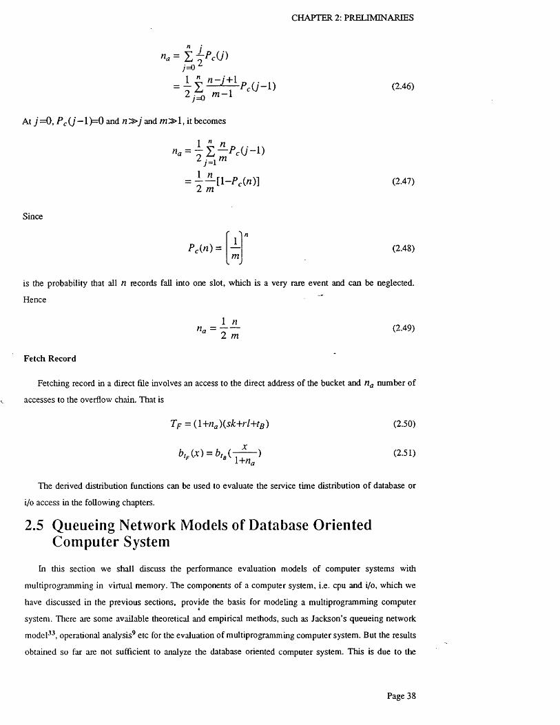
CHAPTER 2: PRELIMINARIES
«„ = E ^ c O ' )7=0
= 7 E £ : : t r ^ 0 ' - l ) (2-46)w i-1
At 7 = 0 , P cO '- l ) = 0 and n ^ > j and m » l , it becomes
2 m
Since
J’cC'O =
1 " nn a ^ - ' L - P c i i - V
j=\
= i — [ ! - ? , ( « ) ] (2.47)
(2.48)
is the probability that all n records fall into one slot, which is a very rare event and can be neglected.
Hence
»a = ~ — (2.49)2 m
Fetch Record
Fetching record in a direct file involves an access to the direct address of the bucket and na number of
accesses to the overflow chain. That is
T p = (1 +na ){sk-\-rl+tg) (2.50)
b,F(x) = bt ( 7 7 — ) (2.51)f 5 1+na
The derived distribution functions can be used to evaluate the service time distribution of database or
i/o access in the following chapters.
2.5 Queueing Network Models of Database Oriented Computer System
In this section we shall discuss the performance evaluation models of computer systems with
multiprogramming in virtual memory. The components of a computer system, i.e. cpu and i/o, which we
have discussed in the previous sections, provide the basis for modeling a multiprogramming computer4
system. There are some available theoretical and empirical methods, such as Jackson’s queueing network
model33, operational analysis9 etc for the evaluation of multiprogramming computer system. But the results
obtained so far are not sufficient to analyze the database oriented computer system. This is due to the
Page 38

CHAPTER 2: PRELIMINARIES
assumption that the cpu and i/o service times are exponentially distributed. This assumption is only
approximately justifiable for cpu bound applications, but is not suitable for i/o bound database oriented
applications. The latter means that queues are usually formed at the i/o devices rather than at cpu service
centre. The distribution functions of i/o service time are proven more likely to be uniform than
exponential. The aim here is to develop performance models for the database oriented multiprogramming
computer systems.
2.5.1 M odel Definition o f C om puter System s
Modem computers very often employ virtual memory technique to manage data storage. The
addressing space of the main memory is called physical addressing. An alternative to physical addressing is
the use of relative addressing which covers the entire file domain maintained by secondary storage such as
drum and disk etc. An application program is free from the actual location of the required data. Instead it
only deals with the relative address of the data. The technique to load the required data from the secondary
storage device into the main memory is called paging. The way of loading and discarding data in the main
memory is called paging discipline. A page is the unit of data transfer.
A paged multiprogramming computer system has two main tasks: memory allocation and scheduling.
Memory allocation by paging is to move address space required by a user into the main memory.
Scheduling is to control an appropriate multiprogramming level by job scheduling algorithm. The purpose
of controlling the multiprogramming level is to avoid deterioration of system performance when main
memory is overloaded.
The two tasks of paged multiprogramming computer system can be naturally decomposed into two
levels, i.e., job scheduling level to control multiprogramming and resource allocation level to control
paging and computing.
At the higher job scheduling level a job from a user terminal is placed into the job scheduling queue
waiting to be multiprogrammed. Only a fixed number of jobs, /V, are allowed to be executed at the lower
level of multiprogramming computer, where N is also the level of multiprogramming. The job scheduling
discipline could be batch, round-robin, last-come-first-serve, etc as studied in section 2 .2 .
At the lower level, a job is always in one of the three states: ready, running and suspended. When the
required address space is allocated by paging, the job is said to be in a ready state. The ready job is placed
on the cpu scheduling queue to wait for execution. A job being executed in cpu is said to be in the running
state. The running will be terminated until either the job’s service is completed or a paging is required. The
cpu execution will be sliced into small slots as studied in section 2.2.1. A job requiring additional page
allocation is said to be in the suspended state, 'the suspended job is placed in the i/o device queue to wait
for the allocation of the required page to the main memory. While a suspended job is waiting for i/o
operation, the cpu is relinquished to process an other ready job in the cpu scheduling queue if there is any.
Since a database-oriented computer system is most commonly i/o bound, queues will be expected to form
Page 39

CHAPTER 2: PRELIMINARIES
at the i/o devices.
We shall now develop the model for a multiprogramming computer system with virtual memory. Two
levels of activities can be modeled by an outer model for the job scheduling queue and an inner model for
the cpu and i/o queues. The inner model represents the multiprogrammed computer with virtual memory;
while the outer model evaluates the control of multiprogramming level. They are illustrated in figures 2.12
and 2.13 respectively.
— r ~| I"! Inner
11 l i Model
Job
SchedulingQueue _____________
Figure 2.12. Outer Model of Multiprogramming Control
The inner model consists of one cpu service centre and m i/o service centres. All of them have the
FCFS queueing discipline. Generally speaking the service time distributions of cpu and i/o devices are
independent and identically distributed. They form a network of queues with a feedback from i/o service
centres to the cpu service centre. The probability of feedback p ^ , determined by the mean number of
paging activities of a job np , is given by
Pfb = -1— = 1 - — (2.52)Up np
Usually A2p » l ; therefore 1. That means the number of activities between the service centres inside
the inner model is much greater than that between inner and outer service centres.
The outer model resembles an aggregated service centre with whatever queueing discipline is used, i.e.
batch, round-robin, last-come-first-serve etc.
2.5.2 D ecom position A pproach with Exponential Serv ice T im es
A number of modeling methods have been introduced to solve the above multiprogramming computer
system based on the assumption of exponential service time distribution. One well known method is the
decomposition approach introduced by Courtois16. The method aims to decompose a complex system into
a number of groups with the assumption that interactions among groups are much weaker than those within
Page 40
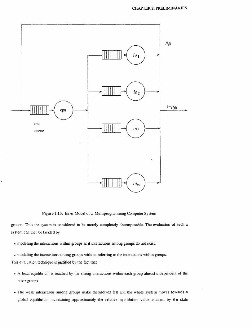
CHAPTER 2: PRELIMINARIES
Pfb
10 i
cpu
cpu
queue
10,
Figure 2.13. Inner Model of a Multiprogramming Computer System
groups. Thus the system is considered to be merely completely decomposable. The evaluation of such a
system can then be tackled by
• modeling the interactions within groups as if interactions among groups do not exist.
• modeling the interactions among groups without referring to the interactions within groups.
This evaluation technique is justified by the fact that
• A local equilibrium is reached by the strong interactions within each group almost independent of the
other groups.
• The weak interactions among groups make themselves felt and the whole system moves towards a
global equilibrium maintaining approximately the relative equilibrium value attained by the state
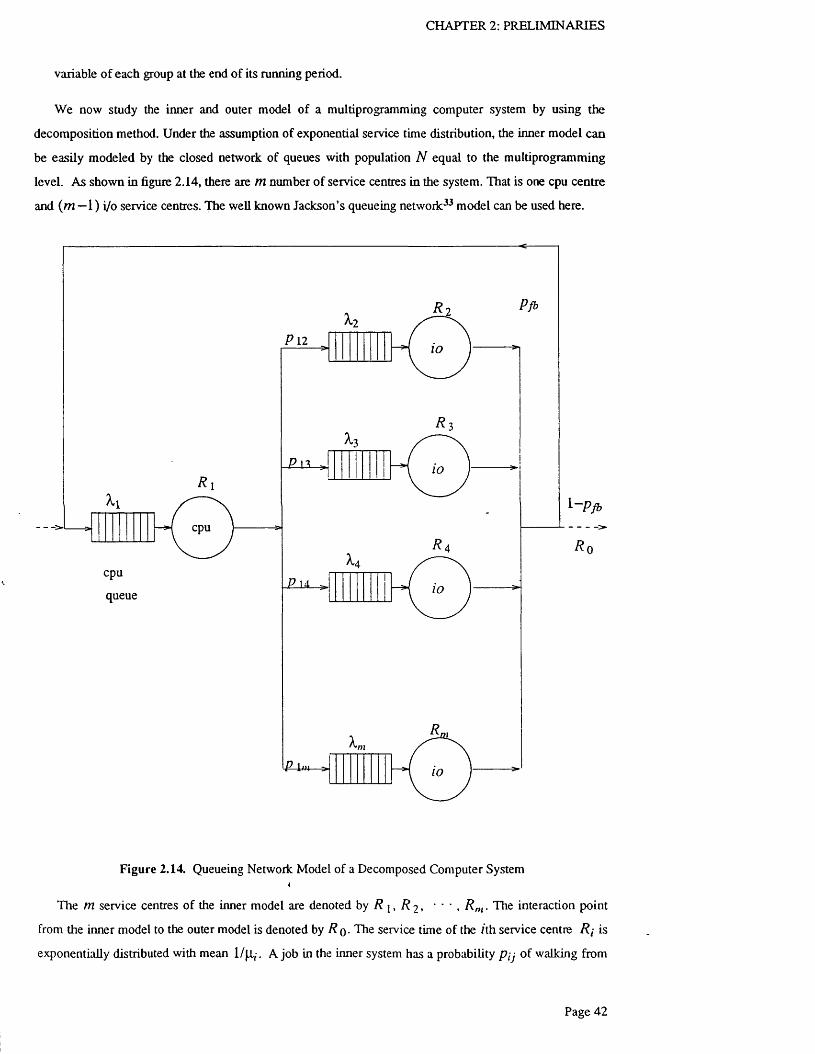
CHAPTER 2: PRELIMINAJRIES
variable of each group at the end of its running period.
We now study the inner and outer model of a multiprogramming computer system by using the
decomposition method. Under the assumption of exponential service time distribution, the inner model can
be easily modeled by the closed network of queues with population N equal to the multiprogramming
level. As shown in figure 2.14, there are m number of service centres in the system. That is one cpu centre
and (m —1) i/o service centres. The well known Jackson’s queueing network33 model can be used here.
P 1210
10
cpuioqueue
10
Figure 2.14. Queueing Network Model of a Decomposed Computer System4
The m service centres of the inner model are denoted by R j , R 2 , ‘ , Rm ■ The interaction point
from the inner model to the outer model is denoted by R o- The service time of the /th service centre Ri is
exponentially distributed with mean l / j l f-. A job in the inner system has a probability p tj of walking from
CHAPTER 2: PRELIMINARIES
centre to centre R j .
P =
> 1 1 P 12 * • * P l m
P 21 P 2 2 * * • P l m
Pm 1 P m 2 * Pmm
(2.53)
is the Markov matrix which defines the probability of the random walk. Under the assumption of the inner
system being decomposable, a closed system of queues, with negligible probability of leaving the inner
system, can be formed.
The matrix P has the property of
= j = l *i = l
The Markov matrix defining the inner model is given by
P =
0 P 12 * • * P l m
I 0 • • 0
1 0 • • 0
ei ~ £ ejPji j = 1
A closed queueing network with exponential service centres has a product form solution
P \ ( n l ) p 2 { n 1 ) • • • p m{nm)P { n u n 2 , • • • ,nm) =
G( N)
(2.54)
(2.55)
where
5 > i , = i
A useful parameter of the closed queueing network is the relative throughput e t i —1, ' • • ,m , which
can be derived from
(2.56)
(2.57)
where P(ji ' ' ' ,nm) ^ l^e steady state probabilities of a network state with m service centres,
Pj(nj ) ( j—l i ' ' ' , m ) are a steady state probabilities o f the state of service centre R j with rij jobs,
G( N) is a normalization factor of the product form solution
G { N ) = X X l ( n l ) X 2(n2) - - X m(nm) « , + • • • + n = N
(2.58)
Page 43

CHAPTER 2: PRELIMINARIES
and Xj{ r i j ) are factors proportional to the steady state probabilities of flj number of jobs in service
centres R j in isolation. Since the service centres of the inner model are single server service centres,
X j ( n ) are given by
X j ( n ) =
The equation for G ( N ) can be simplified as
Myn = 0 , • * • ,iV
G j { n ) = G j - i i n ) + - * - G j { n - 1) , ; '= 2, • • • ,m: n - 1, • • • My
The interarrival rate or throughput of centre R t , denoted by A,-, is given by
e j G ( N - 1)A ; = ------------------
1 G ( N )
The utilization of the server at service centres R j is given by
A ;UJ = —
My
The mean queue length of the service centre R j is
n j ~ ^ i G ( N )
From Little’s formula the mean response time of service centre R ; is
(2.59)
(2.60)
(2.61)
(2.62)
(2.63)
R ; = — 1 A ;
(2.64)
An important system parameter is the marginal distribution of queue length, which can be derived by
P i ( n ) =
(ej/[Lj)n [G CN - n ) - ( e j I \ i j ) G ( N - n - L)]
G ( N )
with a special case of n =N. We have
P j ( N ) = e j / \ i j
Since G (0)=1 and G 0 )= 0 for / < 0 ,
N [G ( 0 ) - ( g j l \ i j ) G ( - 1 ) j
G ( N )
(2.65)
(2 .66)
Page 44

CHAPTER 2: PRELIMINARIES
P .( A 0 = ^ —^— (2.67)A G( N)
Now we shall derive the state dependent aggregated service rate f l (n) o f the inner model. After the
local equilibrium is reached at the inner model, the probability of a job moving from the service centre R j
of the inner model to the point R q at the outer model is defined by PjQ, j — 2 , * ' * ,m, where
P j O ^ P j l
and
P 10=0
The probability of feedback to cpu after paging is given by
Pfb = 1 - — (2.68)nP
Therefore the probability of a job leaving the inner model from service centre R j (J = 2 , ’ * * ym) is given
by
PjO = Pi j Pf b
= (1- — )Plj (.2.69)nP
We have
mPfb = 2 > y 0 (2.70)
;= 2
At the multiprogramming level of n the aggregated service rate of the inner model is equal to
m| i( / i) = ' Z \ i j [ i - P j ( n ) ] p j 0 , n = l,...,/V ;|i(0 )= 0 (2.71)
y=2
The outer model can be easily evaluated as a single server service centre with state dependent service
rate
f JLL(/i ) if n < NM-( /2 )= |^ (A /) if n >N {2J2)
2.5.3 Diffusion A pproxim ation A pproach with N on -exponentia l Service T im e
The application of the conventional Jackson’s queueing network solution is limited by the assumption
of the exponential distribution of service time. In general, the assumption is not well justified, especially in
the case of a database oriented computer system. In such a system transactions are i/o bound and the i/o

CHAPTER 2: PRELIMINARIES
service time tends to be uniformly distributed rather than exponentially distributed. This leads us to
employ the diffusion approximation approach to model the non-exponential servers in a computer system.
We shall still use the decomposition method of the inner and outer model. But here we only concentrate on
solving the inner model by using diffusion approximation method; while the technique for solving the outer
model is the same.
The diffusion approximation method can obtain highly accurate results when the load of traffic in the
queueing network is heavy39, as for the database oriented computer system whose work load to the i/o
service centre is considerably heavy. This method can provide the exact solution in the case of
exponential service time distribution. The basic idea of the method is to approximate a discrete-state
process (e.g. a random walk) by a diffusion process with continuous path. The discrete-state of interest in
queueing network is the number of customers in each state. The probability of a discrete-state n is denoted
by P(n) . It can be transformed to a continuous time-space, i.e., P(n)-* f (x , t ) , where f (x,t) denotes
the probability of X customers at time t.
We first briefly present the diffusion approximation for a single queue, while the detailed derivations
can be found in Lavenberg42. Let A (t) and D (t ) be the cumulative number of arrivals and departures
up to time t respectively. Then the number of customers in the service centre at time t is given by
Q { t ) - A { t ) - D { t ) (2.73)
The change in queue length between time t and t +A£ is
Q { t+ A t ) -Q ( t ) = [A ( t+ A t) -A ( t ) ] - [D ( t+ A t ) -D ( t ) ] (2.74)
or
AQ ( 0 = AA(t ) -A D ( t ) (2.75)
Let the interarrival time and service time be both independent and identically distributed (i.i.d) with (mean,2 2variance) given by ( J I^ O ^ ) and (jLLj, ) respectively. Then according to the central limit theorem, we
can show that if A/ is sufficiently large, many events will take place between time t and t+At. If Q{ t )
does not become zero in this interval, then A Q { t ) should be approximately normally distributed with mean
E[AQ{t ) ] = {V\la- i f \ l s)At (2.76)
and variance
Var [A Q (t )] = (cal\La+c„l\Ls )&r (2.77)
2 2 2 2where Ca=Oa/\la and c s= O s /H s are the coefficients of interarrival time and service time respectively.
The above results lead to the following continuous process X ( t ) as an approximation of a discrete-
state process Q{t ): it is defined as such that its incremental change AX( t ) = X (t+At)—X ( t ) is

CHAPTER 2: PRELIMINARIES
normally distributed with mean fJA^ and variance CC’At, where
and
The density function of X ( t )
Ca Csa = ---- + ----- (2.78)
\^a m
B = —------ (2.79)M-a M'j
/ (x,t)dx = Pr {x<X ( t ) < x + d x } (2.80)
satisfies the Kolmogorov forward diffusion equation. The solution of the diffusion equation is then given
by
f-ye'V if a* >0
/ « = 0 if a < 0 (2'81)
where
2(3 Y = a
_ 2(1 f \ia - l l \ i s )
Cq! Pa ! M-j
_ - 2 ( l - p ) (2 82)Cj p + c 5
and p=fi-J/|i.a is the utility of the service centre.
Let p (n) denote the diffusion approximation to the probability that the queue length is n in steady-
state, then
p ( 0) = 1 -p
p{n) = p ( l - p ) p ” /2>1 (2.83)
A
where p = £ ^ .
Now we shall derive the diffusion approximation equations for the closed queueing network of a
computer system. Applying the single queue solution to the closed queueing network, we can obtain some
interesting results. We shall consider a closed network of queues consisting m single server service centres, . 2
as shown in figure 2.15. The service times at centre I are i.i.d with mean JI/, variance G, and coefficient2 ^C /+ G ;/}l,r , z = l , ' * ’ ,272. The routing path of a customer within the closed system is specified by the
Markov chain matrix probability pij satisfying
Page 47

CHAPTER 2: PRELIMINARIES
P 12.
Pfb
cpu
cpuqueue
Figure 2.15. Closed Queueing Network
mL p u = 1 <2-84>
j =i
The relative throughput of service centre i is given by
mec = X ejPji (2 85>
7 + 1
Similar to the single queue solution, the parameters OC,P and y are defined as matrixes Ct,{$ and y
respectively. If p u ^ Q , CL is a m x m matrix given by
m Qa = X — V*-V* = W (2.86)
where V ^ is an m - dimensional column vector whose h h element is unity and /th element ( i^ lc ) is ~Pki-
Page 48

CHAPTER 2: PRELIMINARIES
That is
V i = [ - P k l - P k l * ' ’ ’ * 1» * ’ ‘ - P k m \ <2 -8 7 )
Matrix w is a non negative definite matrix of m x m whose coefficients are
w i j
Y ,P k i^ -P k i)! \^ k i = jk = 0
m- J ,PkiPkjI\kk i ± j
k =0
(2 .88)
P is an m-dimensional column vector in which the Zth element is given by
mPi = 'L P k i l P ' k - y P ' i 1=1. " • (2.89)
k=Q
Y is an m-dimensional vector given by
Y = 2a-1 p (2.90)
Here we shall introduce a novel method to solve the closed queueing network of diffusion
approximation. The closed queueing network has an approximate steady state discrete probability
P ( n \ > n 2 , * ’ * >n m ) given by
£/ x P\ { r i l )P2{n1) " • P m{nm)P ( n l t n 2 , ■ • ' ,nm) = ------------- — —------------- (2.91)
Lr{Jy)
where P is a factor corresponding to the steady-state probability of the state of the service centre i in
isolation and G (N ) is a normalizing constant given by
G ( N ) = X X l ( n l ) X2( n2) - - X m(nm) (2.92)n I + ' ‘ ‘ +nm=N
and N is the number of customers in the closed queueing network, and
Xj0i j) = (eyi)ni = e nfii (2.93)
Noticing the clear resemblance of the above form to the product form of Jackson’s closed queueing
network, we can similarly obtain the mean measurements and marginal steady-state probability Pj(n) of
queueing length at service centre j .
Invoking the convolution algorithm we have
Gj(n) = Gj - i (n)+eyjG j ( n - 1) /=2, • • • ,m; n= I, * • • N (2.94)
The steady-state probability is given by
Page 49

CHAPTER 2: PRELIMINARIES
P j W =
_ e nyj[ G ( N - n ) - e yjG { N - n - l )] G ( N )
and
,Ny.i, ( N) = - y G (/V )
The mean queueing length is given by
* e ny‘ G { N - n )
(2.95)
= 777777 (296)
The throughput is given by
n: = Y ---------- --------- 1 (2.97)1 n% G ( N )
e : G ( N - 1)A ; = ■ A -- ■ (2.98)
The mean response time is given by
G ( N )
NJR j = ~ T (2.99)
A ;
Referring to the inner and outer model of multiprogramming computer system introduced in sections
2.5.1 and 2.5.2, we can easily derive the aggregated service rate of the inner model with the
multiprogramming level n. That is
m|A (« )= Z V i j [ l - P j ( n ) ] p j 0 « = I , . . . ,N ; JLL(0)=0 (2.100)
7=2
where p j 0 is the routine probability of a job leaving the inner model from service centre j .
PjO = ( l - — ) P l j (2.101)nP
The outer model of the multiprogramming computer system can be evaluated with the given (!(« ) by
the decomposition method introduced in section 2.5.2. The above results will be used in the following
chapters when evaluating computer systems.
2.6 Summary
In this chapter, the methods to evaluate the major components of distributed databases, i.e. cpu, i/o and
computer network, have been presented. Decomposition and diffusion approximation methods have been
used to model database-bound multiprogramming computer systems.
Page 50

Chapter 3. Concurrency Control Model of Centralized DB
3.1 Introduction
The problems associated with the evaluation of centralized databases have been extensively studied in
recent years. In particular, the locking problem of centralized databases has received much attention and
substantial research efforts have been made to evaluate the performance of locking mechanisms. However
the following problems still have not been solved. The most difficult one associated with locking is to
evaluate the waiting time upon locking conflicts. This is mainly because of the stochastic nature of the
waiting time, which depends on the behavior of the departure process of transaction execution. Another
problem associated with locking is the queueing discipline, which often means that the lock manager can
apply preemptive priority scheduling over the transaction executions. The difficulty of evaluating locking
performance of a multiple class transaction system is also widely recognized; this is due to the fact that the
overall system performance depends on not only different service demands but also different lock conflict
rates and waiting times of multiclass transactions. In this chapter a unified analytic model is introduced to
solve the above problems. The model can apply to both open and closed database systems with either
single class or multiple class transactions49.
Section 2 represents the specification of the concurrency control and locking algorithm. Section 3
introduces the analytic model to evaluate the waiting time of the blocked transactions and priority queueing
in an open system. Section 4 applies the waiting model to a closed system. Section 5 introduces the method
to evaluate multiclass transactions. Section 6 validates the analytic results with the simulation results
obtained by Ries and Stonebraker68.
3.2 Model Specification
3.2.1 B asic T w o Phase Locking
Bernstein and Goodman8 have given a very thorough survey of the concurrency control algorithms in
database systems. It is therefore appropriate to provide only a brief discussion here, while the detail can
be found in their paper.
Two phase locking is based on the concept of detecting and preventing conflicts between concurrent
operations. The unit of data is protected by locks. A read transaction has to own a shared lock before
actually performing the operation. The write transaction has to own an exclusive lock before writing data to
the database. A shared lock can be owned by many read transactions; while an exclusive lock can only
belong to one write transaction.

CHAPTER 3: CENTRALIZED DATABASES
A transaction is said to be in a lock conflict state if one of the following situations happen: for read-
write synchronization two locks conflict if one is a shared lock and the other is an exclusive lock, and both
locks are on the same data item; for write-write synchronization two locks conflict if both locks are on the
same item and are exclusive locks.
The correct execution of locking is governed by a concurrency control algorithm. With two phase
locking, a transaction requests locks in a growing phase and releases locks in a shrinking phase. Upon lock
conflict, a collision resolution algorithm needs to be used to deal with the scheduling of the blocked
transactions. If the required locks are denied in the growing phase, the transaction will be scheduled for
retry according to the collision resolution algorithm used. When locks are released at the shrinking phase,
the blocked transactions waiting for the locks are dealt with according to the collision resolution algorithm.
3.2.2 Collision R esolution Schedu ling A lgorithm
A number of collision resolution scheduling algorithms have been introduced28,83. They can be mainly
classified into two categories: the fixed waiting algorithm and the scheduled waiting algorithm. The fixed
waiting collision resolution algorithm is to restart a blocked transaction after a fixed period regardless of
the availability of the locks, while the scheduled waiting algorithm is to free blocked transactions as soon
as the required locks become available. As stated in chapter 2, most researches have been carried out in
evaluating the fixed waiting collision resolution algorithm of the centralized system. The scheduled waiting
algorithm is not well studied. It is the purpose of this chapter to address this problem.
The scheduled waiting algorithm is as follows. When a transaction encounters conflict locks at the
growing phase, it enters a blocked transaction queue and all the conflict locks are recorded. When locks are
released at the shrinking phase, the blocked transactions and their conflict locks are checked against the
released locks. The blocked transactions will be freed if all the required locks become available. The freed
transactions then compete for their locks at their next growing phases. The more detailed description of the
algorithm can be found in Ries and Stonebraker’s paper68, in which they used a simulation model to
evaluate the performance of a centralized database.
The implementation of scheduled waiting algorithm involves setting up a hash table, in which each
item is consist of a lock and a list o f the transactions waiting for the lock. Setting up locks involves
checking the hash table for the corresponding lock items; if all the locks are available, the transaction can
grant the locks by locking them in one atomic operation. Once a transaction is completed the database
management system releases the locks in the hash table. The blocked transactions associated with the
released locks are therefore freed28.
3.3 The Scheduled Waiting Model in an Open System
A database system can usually be accessed by a number of users simultaneously via local or remote
terminals. We can consider users’ requests as a steady stream of jobs arriving to the database. Each of the
Page 53

CHAPTER 3: CENTRALIZED DATABASES
jobs requires certain amount of database service. Such a system can be naturally considered as an open
database system in which transactions arrive at the source of the system and depart at the sink as shown in
figure 3.1. As introduced in chapter 2, a database system is composed of cpu and i/o devices. They can be
modeled by a queuing centre using decomposition method, introduced in section 2.5. A transaction
re q u ire locking and execution operations will be processed by the computer system.
In an open database system, a transaction first requests locks at cy. If all locks are granted, the
transaction is executed at ce , and releases the locks and leaves the system; otherwise the transaction is said
to be blocked and put into the blocked queue at b. The blocked transaction in the blocked queue will be
freed when the required locks are released. It then re-enters C/ to request locks again. The lock request and
transaction execution share the same computer resources. The locking operations have priority over the
execution operations, which means that the lock request operations are processed by a computer with
higher priority over the transaction execution operations.
blocked
queue
dQck release
lock
request execution
high priority✓
' low priority
computer
resources
Figure 3.1. Locking Model of an Open Database System
We shall now derive the throughput of the locking model shown in figure 3.1, where the throughput at
C/, c e and b are denoted by A /*\ A ,^ and A>b respectively. The interarrival rates at the source is denoted
by Xq. Let us define pb as the probability that4a transaction can not grant all the required locks, therefore
must enter the blocked queue at b\ and <lb= ^~Pb probability that a transaction can grant all the
requred locks. It can be seen that under steady state
Page 54

CHAPTER 3: CENTRALIZED DATABASES
A,(1) = Xq + Xh
A(2) = Ao
h = P b ^ a )
and Xfy can be rewritten in terms of Xq as
^ 0
l~ P b
and
Xu —
Pb^O
l~P b
(3.1a)
(3.1b)
(3.1c)
(3. Id)
(3.1e)
blockedqueue
computer
high prioritylow priority
Figure 3.2. Queueing Network Model of an Open System
Since lock request and transaction execcution share the same computer resources as shown in figure
3.1, we can reconstruct the locking model into a queueing network model with priority queueing discipline
as shown in figure 3.2. The computer resource is represented as a single server service centre. Lock request
is served with first class priority; while transaction execution is served with a second class priority. The
arrival rate of the first and second class transactions are given by X^ and X ^ respectively. Since the
waiting in the blocked queue does not require computer resources, it can be modeled as an infinite-server
service centre. That is each blocked transaction is served immediately for a period determined by the
availability of locks.
As discussed before, the problem associated with evaluating locking performance is very complicated
because of its stochastic nature. The waiting time analysis can not be isolated from the rest of the system.

CHAPTER 3: CENTRALIZED DATABASES
It depends on the system throughput, the number o f locks already held, and the number of locks in the
waiting centre. The stochastic nature of the blocking process is strongly related with the departure process
of the transaction execution, i.e. the second class priority customer in fugure 3.2. The prime goal here is to
obtain the characteristics of the departure process of the second class customer.
To enable meaningful analysis, we assume that the interarrival process is Poisson. The service time is
independent and identically distributed It is appropriate to treat the computer service centre C as a
preemptive resume priority for M I G I I with two priority levels. Strictly speaking, the computer service
centre c is not an independent M I G 11 queue; the whole model should be treated as a queueing network
because of the effect of feedback. However under the following assumptions the computer service centre C
may reasonably be approximated by an independent M I G 1 1 queue with two priority levels. Firstly we
assume the lock overhead is small. In a real system the lock table is usually maintained in a hash table
either in main memory or on disk. The time spent to fetch certain items from the hash table is very small
compared to the time spent in the transaction execution operations83. Secondly we assume that the
probability of lock conflict is small. In a real database system with a scheduled waiting collision resolution
algorithm, only the transactions in the execution state hold locks. The transactions in the blocked queue do
not hold any locks. Furthermore only those blocked transactions which can grant all the required locks are
allowed to re-enter the system; others must wait until such moment comes. Therefore the probability of
lock conflict is small in most cases.
In figure 3.2, transactions first arrive with a Poisson distribution and enter the computer queue as a high
priority customer. Since we assume that the lock overhead is small, the interarrival times of transactins are
much greater than the service times for lock request, which means that there is almost no queueing of first
priority customers. Suppose Tn denotes the epoch of the /7th arriving high priority customer and S n
denotes the service time of the /7th customer of first priority. Since there is almost no queuing for these
customers, the departure epoch of the /2th high priority customer is approximately equal to { tn+ 5 n }.
According to Doob21, if 1n is Poiss.on and S n is independent and identically distributed, the instants
{T„+.S„ } forms a Poiss on process. We can therefore say that the output process of the high priority
customer is approximately Poisson.
Since we assume that the probability of lock conflict is very small, the effect of feedback should be
very weak. Futhermore since the output process of the high priority customer is approximately Poisson and
the blocked queue is an infinite-server service centre, the output process of the blocked queue is also
Poisson. Therefore it also forms a Poisson input to the computer service centre.
The input process of the low priority customer, i.e. the transaction execution customer, is formed by the
ouput process of the high priority customer,‘i.e. lock request customer. It is therefore approximately
Poisson. The low priority customer, i.e. transaction execution, is only served once and will not cause any
feedbacks.
Page 56

CHAPTER 3: CENTRALIZED DATABASES
As introduced in section 2.5 a computer system with a compound cpu and i/o can be modeled by a
single server queue. Therefore an open database system can be represented by a the M I G / 1 preemptive
resume priority queue with two priority levels. The characteristics of particular interest are the departure
process of the second priority customer; since this process determines the entire waiting process at the
waiting centre.
The following equations are derived to obtain the Laplace-Stieltjes transform of the distribution
function of departure process of the second priority customers.
We shall describe the z’th priority levels as (z). If i <j\ the customer of zth priority level will have
priority service over those of j th level. The distribution of the interarrival time for the zth priority customer
is supposed to be exponentially distributed with mean and variance the distribution of the service
times of the zth priority customer is indicated by H ^ \ t ) with mean
oo
Ji(f) = J t H {l)( t ) d t (3.2)o
and second moment
oo
cj(,)= j f 2 / / (0 (f)d r. (3.3)o
Let us define as the stochastic process of the number of customers of the zth priority level in the
system at the time t when the /zth customer arrives. We shall first prove in the following theorem that the
departure process of the second priority customer is Markovian, which means that the time interval of two
successive departures of the second priority customers, i.e. transaction execution customers, is independent
and identically distributed. This property is very important to a stochastic variable as it is a necessary
condition of a proper distribution function used in queueing networks. The proof can be found in appendix
B.
Theorem 3.1: The process [0 ,°°)} which is regenerative with respects to the renewal precess
of the interdeparture time of the second priority customer is Markovian.
In order to obtain the distribution function of the departure process of the second priority customer we
need to employ the concept of completion time of a customer, which was introduced by Cohen15. This is
the time between the epoch when the service of a customers begins and the first epoch thereafter at which
the server becomes available to another customer. The completion time of a second priority customer is
denoted by Ct .4
The Laplace-Stieltjes transform of the completion time (?,• of a second priority customer with
preemptive resume priority discipline is given by15
Page 57

CHAPTER 3: CENTRALIZED DATABASES
E { e JCi) = £ j e - 1' (* \ >f) g~x" W 2)a)(H.(1>(*, 1 ))‘k = 0 0 k -
= P<2 ) (s+ X ( 1) ( l - n (1)( ''. 1 ))) . R e i> 0 , (3 .4 )
with
|3 °-)( s ) = \ e - s,d H a- \ t ) (3.5)0
and 1) defined as the Laplace-Stieltjes transform o f the busy period of the first priority level.
(S , 1 ) is the zero with the smallest absolute value of
z = { s + C l-z jA ,^ } , R e 5 > 0 (3.6)
with
p(1)(s ) = (3.7)
{x (2) > 0 1 X{1)=0 } {x{2)<0 1 x (1)= 0 }
Figure 3.3. Epochs of the Second Priority Customers
We further introduce the concept of pie-waiting time of the second priority customer, denoted by Wz.
This is the time between the epoch at which the server becomes idle and the first epoch thereafter at which
the service begins to serve a second priority customer. This equals to the idle period of the system plus the
residual busy period of the first priority customer. In order to have a clearer picture of the M I G / I queue(2 )with two priority levels, figure 3.3 illustrates the epochs of the second priority customers. T), denotes the
departure epoch of the /2th second priority customer and rn denotes the epoch at which the /2th second
priority customer starts to be served. If before epoch the (/z + L)th second priority customer has
already arrived, i.e. > 0 | t h e server starts to serve the (/2 + l)th customer immediately.
This period, i.e. from to is exactly the completion time of the second class customer15. If
however at the epoch the (/2+ 2 )th second priority customer has not yet arrived, i.e.
{X(2 )< 0 |% ( 1)= 0 }, the server will spend a pre-waiting time w z- to wait for the arrival of the ( /z+ 2 )th
second priority customer and the comple rion time of the first priority customers before the service to the
(/z+ 2)th second priority customer begins. Since from the epoch to the first epoch the (/z+2)th

CHAPTER 3: CENTRALIZED DATABASES
second priority customer arrives is the residual interarrival time of the second priority customer, denoted by
0 ^ . The period from the epoch of the arrival of the (/z+ 2)th customer, i.e. 'T ^ + i+ 0 ^ to epoch of the
completion of service of the first priority customer is the the residual busy period of the first priority
customer, denoted by Thus the pre-waiting time W/ is composed of 0 ^ and b ^ \
Since the interanival process of the second priority customer is Poisson, the residual interarrival time is
equal to the Poisson interanival time with mean 1/A/2 . The Laplace-Stie|es transform of 0 ^ is
The residual busy period b ^ starts with a initial waiting time \ ) ^ which is equal to the virtual
iting time <
Cohen that15
waiting time of the ^ - system at the epoch t at which the second priority customer arrives. It is due to
E { e sb0>} = j J e x p [ - { ls-+A.(1)( l - j i ( 1)Cs', l ) ) } o ] *fo / >r{ \)^ 1) < a | ,u[)1)= 0 } e xu>td X {2)tr=0a = 0
_ x (2>- s + x .(1)[)i(1)a , n - i x a ) (A.(2), i ) i
- [x.( 1)+ x < 2) - x u y i , (A.C2) , n ] ( i - s A . (2 )) (3.9)
Now we can form the pre-waiting time of the customer of second priority level. That is
w z = 0 (2 )+Z>(1) (3.10)
From (3.8), (3.9) and (3.10), we have
E ( e - " ,i I = £ ( e - s0<2>) - E f e - sb"' I
J+ X (2) [X( 1)+X(2>- X cl)| i ( 1) (X(2>, l ) ] ( l - .s /X (2))
if R e s > 0.
(2) (^)The following derivations aim to obtain the distribution function of the departure time ,l n +i—
the second priority customer which can be presented by C; and w t . As we can see from figure 3.3, if a
second priority customer leaves the system with at least one second priority customer in the queue, i.e.
{X ^ I } * the interdeparture time ^ n l l ~ * s equal to the completion time of the next second
priority customer. If however the /2th second priority customer leaves system empty, i.e.
1x ^ = 0 } the interdeparture time between the nth and ( /z + l) th departures is the sum of the
completion and pre-waiting time of the next arriving second priority customer. Thus the inter-departure
time can be given by
Page 59

CHAPTER 3: CENTRALIZED DATABASES
^n + l - ^ n = C i + i
w «’ if {%(2)= 0 | x (1>=0}
0 if {%(2)> 0 | x (l)=0}
(3.11)
This can be rewritten as
Pr <t | = Pr {%(2)=01 X(L)= 0 )Pr {c ; < t ) *Pr | w ; < t )
+ (!-? /-{X<2)=01 X(1)= 0 ) )Pr {Ci < t)
For the stationary process it follows that
l i m / >r { x (2)= 0 | x <1)= 0 ) =l - a
t —$ oo l - a ( l )if a < l
(3.12)
(3.13)
and
l im />r{x(2,> 0 | x (1)= 0 )=, ( 2)
t — i OO
where
and
l - a
a w = X l>p.w
a (2 ) = x « y 2 >
a = a (1)+ a (2).
( l )if a < l (3.14)
(3.15a)
(3.15b)
(3.15c)
Let us denote g (.S') as the Laplace-Stieltjes transform of the density function of the departure process of
the second priority customer. We have
* —r(T<2> — t <2>1g (.s ) = E { e s[Xn+l T" '}
1 —a , —sc; , _ , —sw j, a _ . —sci, ( 2 )
- E { e ' ) E { e * }+- ■E{el - a (1) 1 ’ ' l - a (l)
P ‘ 1 U ’ *+X® [^ 1>+V2)- ^ 1V<1>(^2>,l)](l-i/X<2)). ( 2)
+ a
= p (2) { ^ (l)( i - n (1)(5, 1))) L - a (1)
( \ \ ’ a.(2) ' ' x (2» ' x.(2)- i + x (1)[n(2,( i , d - h(1)(>.<2). D] i /.(2)( l - a )X.(2)+ i \<2>-.s X(1»+X(2)-X<1>H<1»(X<2),1 )
t a (3.16a)
Let us denote jda as the mean interdeparture time of the second priority customers. We have
Page 60

CHAPTER 3: CENTRALIZED DATABASES
d * /rv.= (° i
(3.16b)
s = 0
For exponential service time, the mean service time of the inter-departures process of the second priority
customer can be further derived as follows. Since
i
H<2 > * + 1
- f r ( 1)(*. i )d s
s —0
d_
d s
_
— 7 — (ji(1^ + a (1)+ l -V ( jx (1)^ + a (1)+ l ) 2 - 4 a f ^ ”) 2a (1) s =0
(1)
l - a (1)(3.17)
and
n ( 1) ( s , n = - L - ( ji( 1, j - k j (1)+ i - V l)^ cl>+ i ) 2- ^ (1 ) )3^=0 2 a ( * ;=0
= 1 (3.18)
we can obtain
I1(2)
+l - a
where
2 a (1) L
(3.19)
(3.20)
In order to build the database waiting model we also need to obtain the residual inter-departure time of
the second priority customer. It is due to Cohen that15 for the stationary process, the Laplace-Stieltjes
transform of the residual lifetime density function for the inter-departure process of the second priority
customer is given by
(3.21)
From the Laplace-Stieltjes transform of the density function of the inter-departure process of the
second priority customer g ( s ) we can easily obtain its mean. That is
Page 61

CHAPTER 3: CENTRALIZED DATABASES
1 d |xa = - — lun — 1 - ? CO
2fJ-a d s 2g (0 ) (3.22)
The above results are very important and crucial to the evalution of scheduled waiting in a blocked
queue. It is the most important step in the derivation of the blocking model. It reveals the mean and
distribution of the departure process of the transaction execution job. Since the release of locks from the
completed transactions triggers the release of the blocked transactions. The above results, therefore, define
not only the mean waiting time but also the stochastic nature of the blocked transactions, which has not
been solved before. Previous researches can only evaluate fixed waiting time from approximate estimation,
as in T ay’s paper, or even from empirical measurement, as given by Irani. Our result, on the other hand,
provides exact evaluation of blocking with scheduled waiting collision resolution algorithm.
Blocking Model
We shall now derive the formulae for the waiting model of open database systems based on the inter-
departure process of the second priority customer. The waiting time of the blocked transaction is closely
related to the inter-departure time of the leaving transactions. We shall first derive the waiting time in the
blocked queue and then the probability of locking conflict.
The performance model of a database system, as discussed in section 3.2 is constructed by an open
network of queues with one computer service centre and one blocked transaction waiting centre. Each
transaction starts with going through the computer server with a preemptive resume priority to request, set
or release locks. Once a transaction gets all the required locks, it goes straight back to the computer server
to be executed with a second class priority. After the execution the transaction finally departs from the
computer server and releases all locks. From the point of view of the computer server each departure of its
second priority customer will release r locks, where r is the average number of locks held by one
transaction upon execution. Therefore the waiting time for each release of r locks in the blocked queue is
equal to the inter-departure time of the second priority customer in the computer service centre.
From theorem 3.1 it follows that the departure epochs of the second priority customer are the( 2 )regenerative points of the %) - process. Consequendy, the inter-departure times of the second priority
customer are independent and identically distributed variables with the Laplace-Stieltjes transform of the
density function given by g ( s ) in equation (3.16a).
As shown in figure 3.4, the waiting time for each lock release can be naturally modeled by a waiting
phase. A blocked transaction goes through one or more waiting phases before finally obtainhfil the required
locks. It should be noted that the service time of the first waiting phase is the residual time of the
interdeparture process of the second priority customer in the computer service centre, because the initial
arrival of a blocked transaction in the waiting centre is independent of the starting point of the departure

CHAPTER 3: CENTRALIZED DATABASES
process. In the subsequent waiting phases the waiting time is exactly equal to the interdeparture time o f the
leaving transactions. Thus the service times of the start phase and the subsequent phases in the waiting
model are independent and identically distributed with their Laplace-Stieltjes transform of the distribution
functions given by g ^ ( s ) and g (S ) respectively.
Figure 3.4. A Phase Method of Waiting Time in the Blocked Queue
The above model of waiting time in the blocked queue can be further aggregated into an single
infinite-server service centre, which can be easily evaluated in the numerical calculation of the overall
model. As shown in figure 3.4, a blocked transaction first enters a start phase which is defined by g ^ (S ).
At the end of the first phase, r locks are released by a leaving transaction. Then the blocked transactions
either leave the waiting centre with probability p i or enter the second phase of waiting with probability
q i and so on. That is upon leaving the jxh phase, a blocked transaction enters the / + l t h phase withA A
probability q j and leaves the blocked queue with probability p j . We shall now determine the probability
P j of phase j . Let us define L as the total number of granules in the database. (Granular is the unit of
data, which can be locked.) Before a lock release, there are N i locks held on average. At the epoch of the
completion of each phase there are r locks released from a pool of N[ locks. Therefore the probability of a
transaction to successfully granting r required locks becomes
N j - rq j = ( 1 j ~ Y (3.23a)
and
P j = 1 - 9 ;
Since all q j ( j = [ , • • ■ ) are equal,
~ , , ^ > ~ '\rq j = q = ( l — ^ - y , (3.23b)
and
Pj = 1 ~ q (323c)
Page 63

CHAPTER 3: CENTRALIZED DATABASES
Based on Cox’s method of phases18 the service time of the waiting centre has the Laplace-Stieltjes
transform function in the form of
fb(s) = plgl(s)+q1p2gl(s)g*(s)+qlq2P-igi(s)g*(s) + - ' '
(3.24)= E j= i
t , 1*n <?<i = l
Substituting (3.23a), (3.23b) and (3.23c) into equation (3.24), it becomes
f b ( s ) =j =1
_ (1 - q ) g \ ( s )
1 - q g \ s )
Substituting (3.21) into the above equation, it can be rewritten as
/6 ( 5 ) = M x ! z s M
^ ( l - ^ g (5))
Since the mean interdeparture time of the leaving transactions equals to the mean interanival time of the
transactions, i.e. = l / | I a , we have
^ x Ao(l-$)(l~ g \ s ) )fb (s ) = ------------ — ----------- (3.25)
s ( l - q g (s))
The mean service time of the waiting centre is given by
(3.26)M* = - £ f b (s )5 = 0
Now we need to to obtain the probabilities of lock conflict, when a transaction first acquire locks. Two
parameters are used to define the lock conflict rates: q, the probability of successfully granting one lock,
and P b , the probability of lock conflict upon requesting r locks. We also have
qb = l~P b (3.27)
Under steady state, the number of locks held is taken as the mean number of transactions in execution —(2)
:e, i.e. n , multipled by the mean i
of locks held in the system is therefore
_ ( 2)state, i.e. n , multipled by the mean number of locks required by each transaction. Thus the total number
Ni = r - n {2) (3.28)
Considering a database as a universe containing a total number of L granules with N[ locks already held, a
transaction requests one more lock will have a probability
Page 64

CHAPTER 3: CENTRALIZED DATABASES
'Ni- rL —iTT
L
(3.29)
of being conflict with N / locks already held. Therefore the probability of successfully granting one lock
becomes
ffy-I) L - 1
q = 1
L
_ 1 Nl _ l rvT(2)L L
(3.30)
The probability of a transaction successfully granting all the required r locks can be written as
:(2)'
qr = l -r-n
and the probability of lock conflict upon requesting r locks is therefore
Pb = i -qr= l - l -
- ( 2)r -n(3.31)
and
qb = l - P b
1 -- ( 2)r-n
(3.32)
We shall now derive the mean measures of the open database system. A lock manager always receives
the first priority service with preemptive queueing discipline. Therefore it has the same characteristics as
the M / G / l queue. The mean waiting time of a M /G / l queue is equal to15
,( 1)„U ) rrd )(3.33a)
2 1 - a < ‘> (nM>y
where is the second moment o f the distribution Therefore the mean response time of a lock
manager is given by
■ m 1 a{lV l) ^U)+ L( 1) (3.33b)
2 l _ ^ d ) (flCl) ) 2
It is due to Cohen13 that the mean waiting time of the second priority' customer with a preemptive resume
Page '65

CHAPTER 3: CENTRALIZED DATABASES
queueing discipline is given by
vvr(2) = r d ) r(2)+
2 ( l - a (1)) ( l - a ) A,(1) A,(2)(3.34a)
It is obvious that the mean response time of a transaction execution customer is equal to the mean waiting
time plus the mean service time of the second priority customer. That is
R & =1 «U> r(2 )
+ (2 ) (3.34b)
Consequently the mean queueing length of a lock manager is given by
(A.c l))2 a (1>
2 ( l - a (1>)
and the mean queueing length of a transaction execution customer is given by15
(3.35)
1 0 <‘>- + •
X<‘> X<2>(3.36)
Now we have derived all the equations necessary to evaluate the mean measures of the waiting model
in an open database system. It should be noted that if the service time distribution of the computer server is
exponential, the mean measures obtained from the above equations are exact, if the computer service time
is independent and identically distributed, the above results are approximate. Since the approximation is
made only on the assumptions of small lock overhead and lock conflict rate, it can be easily justified by
most real database systems. Furthermore the assumptions only effect the distribution characteristics o f the
output process of the first priority customer rather than its means, the evaluation of the overall system
performance is accu*t&,at least to the first order level.
As discussed in the introduction, the analytic models of blocking introduced by others only give an
approximate estimation of fixed waiting78’77. In this section we have derived the model for not only
evaluating the scheduled waiting in the blocked queue with two priority levels but also providing accurate
mean and distribution fuction of waiting time in the blocked queue. We have introduced a method which
can solve one of the most difficult and fundamental problems of blocking, i.e. evaluating the intetdeparture
process of transaction execution. By obtaining the characteristic of the interdeparture process, the waiting
time in the blocked queue is evaluated by using the method of phases. The evaluation therefore has taken
many more fundamental factors into account, such as the stochastic characteristics of the transactions, the
service time and interarrival times of the transactions, the queueing discipline, the collision resolution
algorithm, the structure of locks, etc. It represents the blocking phenomenon much more accurately. It can
be seen in the validation section that the analytic model produces a very accurate ag reement with the
simulation results.
Page 66

CHAPTER 3: CENTRALIZED DATABASES
3.4 The Scheduled Waiting Model in a Closed System
A closed database is a system with a fixed number of transactions repeatedly com peting^ ardware and
data resources. The hardware resources are cpu and i/o devices; and the data resource is a software
resource defined as a collection o f conceptual data divided by a number of granules.
For the closed system with two priority levels, even if the service time distribution is exponential the
conventional queueing retwork method introduced by Baskett6 is still not applicable. We need to introduce
novel method to solve the problem. In this section we shall introduce an approximation method based on
the open database model introduced in the previous section.
In order to compare our analytic results with the simulation results obtained by Ries and Stonebraker68
we built a closed database system according to the specification given by Ries and Stonebraker. In their
model the computer system is composed of a cpu and an i/o device. They can be respectively modeled as
the single server service centres with two priority level FCFS queueing discipline. In the closed database
each transaction starts with receiving cpu and i/o services to request locks. If all required locks are
granted, the transaction succeeds with requesting cpu and i/o services for transaction execution. Otherwise,
it goes to a blocked queue to wait according to the scheduled waiting collision resolution algorithm. After
completing the execution, the transaction releases all its locks and starts again. Here we suppose the think
time is zero. However it is not difficult to include it. As assumed before, the lock manager has preemptive
power over transaction management for the cpu and i/o resources.
The whole system illustrated in figure 3.5 can be modeled by a closed queueing network with a total
number of transactions equal to N , where N can also be interpreted as the multiprogramming level.
We shall now derive the throughputs of the locking model shown in figure 3.6, where the throughput at
C/, Ce and b are X ^ and Xb respectively. Let us define X^pU and X^'J as the interarrival rate of the
Ith priority customer at cpu and io service centre respective and Xq is the overall throughput of the closed
system. It can be seen that under steady state
+ h (3.37a)
K 2pu = U V = Ao (3.37b)
Xb — P b “X\o (3.37c)
A-ipn. A S a n d Xb can be rewritten in terms of Aq as
AS-pl = X ] ^ = (3.37d)l -P b
and
Page 67

CHAPTER 3: CENTRALIZED DATABASES
blocked
queue
' 4Qck release
lockrequest
''execution
cpulow priority
cpu
resources resources
F igure 3.5. Locking Model in a Closed System
, P b h :A* = ------- (3.37e)
1 ~Pb
Since lock request and transaction execcution share the same computer resources, i.e. cpu and i/o
devices, as shown in figure 3.5, we can reconstruct the locking model into a queueing network model with
priority queueing discipline as shown in figure 3.6. The cpu and i/o resources can be represented as single
server service centres. Lock request is served with first class priority; while transaction execution is served
with a second class priority. Since the waiting in the blocked queue does not require computer resources, it
can be modeled as an infinite-server service centre. That is each blocked transaction is served immediately
for a period determined by the availability of locks.
Let us further define the e t as the relative throughputs of service centre i in respect to the throughput of
the closed system, i.e. X<). We have
\ = e{kq (3.38)
Substituting the above equation into equations (3.37b), (3.37d) and (3.37e) we have
Page 68

CHAPTER 3: CENTRALIZED DATABASES
blocke<queue
cpu
'lO lOcpu
cpu
Figure 3.6. Queueing Network Model of a Closed system
= e $ = 1 (3.39a)
e t y u = e $ = - ± - (3.39b)1 ~Pb
Pbe b = ------- (3.39c)
l - P b
We shall apply the method introduced in section 3.3 in the open database system to evaluate the waiting
time in the blocked queue. In the closed system the stochastic nature of the blocking process is determined
by the departure process of the i/o transaction execution centre. As described previously in figure 3.6,
transactions are executed in the service centers with second priority; while lock requests are processed with
first priority. Due to the complexity of the closed queueing network with priority queueing discipline, we
assume that the service times are exponentially distributed. In this section we mainly concentrate on
solving the problem of priority queueing of a closed database system. The Laplace-Stieltjes transform of
the distribution function of the inter-departure process of the leaving transactions can be obtained from
equation (3.16a); and the Laplace-Stieltjes transform of the distribution density function of the blocking
delay in the closed system can be obtained from equation (3.25).
We shall first prove that under the condition of low lock overhead, i.e. < 7 ^ —>0 and exponential
service time distribution of cpu and i/o servers, the inter-departure distribution of the second class priority
customer is approximately exponentially distributed with mean equal to 1/X52\ That is
G ( t ) = l - e ~ Xi2)t (3.40)
We first obtain the busy period distribution of the first class priority customer. From equation (3.6) we have
Page 69
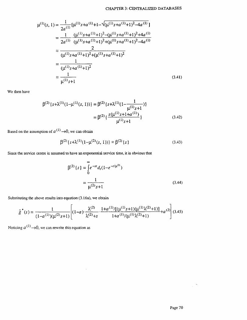
CHAPTER 3: CENTRALIZED DATABASES
H(1)(s, 1) = - 4 — [^(1)i+ a (l)+l-V(u.(1)f+ a(1)+ l)2-4 a (1)]2 a ' ’
_ 1 (}X(1)5-h3(1)+ l ) 2-(tX(1)^+<7(1)+ l ) 2+4<7(1)
2 a ^ l) ( | i ( 1)5 -h3(1)+ l ) 2 -KjJ.(1^+ < 7(1)+ l ) 2 -4<3(1)
2_____________~ (^ (l)5+<7(1)+ l ) 2-K^(1)5+fl(1)+ l ) 2 1
(}X(1)5-k2(1)+ l ) 21
~ p w j + l
We then have
P < 2 ){ i + X (1 ) ( l - H ( 1 ) ( i , 1 ) ) } = P ( 2 ) {J + X .C1)( 1 -------) }p.(1).S+l
_ p m , .?(M-(1)^ + l + g ( 1 ) ) 1
P ' n<‘)* + l '
Based on the assumption of £ 7 ^ —>0, we can obtain
P(2){j+X (1)( l - p . (2)Cs, l ) )} = p(2){j}
Since the service centre is assumed to have an exponential service time, it is obvious that
oo
P ( 2 ) { J ) = / < ? - " r f ,(
|i(2).s+l
Substituting the above results into equation (3.16a), we obtain
g (?) =( l - a i l ) )(\ii2)s + l )
Noticing —>0, we can rewrite this equation as
(3.41)
(3.42)
(3.43)
(3.44)
(3.45)
Page 70

CHAPTER 3: CENTRALIZED DATABASES
1
'(1
X ® + *
X(2)(l+lx(2M
( l - a (l))( |i(2)s + l) \ (2)+ s
X‘2>
( l - a (1))(X(2)+.s)
X(2)
X ® + i
Therefore approximately
G { t ) = 1 - e - X (2)r
This result is very useful. It means that the output process of the leaving transactions is approximately
Poisson; therefore the interarrival process of the transactions in a closed database is always approximately
Poisson. We can thus treat the cpu and i/o service centres in the closed system as M / M / I queue with two
priority levels. This result can be used in not only scheduled waiting but also fixed waiting. Previous
researches only gives an estimation of fixed wiating time on the basis of deduction as in Tay’s work. The
above result provides the mean and distribution function at the accuracy of first order. The result also has
an extremely simple and desirable form which can be easily used in the overall model.
A *
The mean service time of g (.S'), i.e. Jl0 , can be directly obtained from equation (3.40). In order to
prove the consistency of the approximation, we can also derive the mean time between departures from
equation (3.19). We have
(2 )-+
1 —a 1
l - a {l) (1 - a (1))2(2 )
•+1 - a li(1)A<2)+ l
l - ^ l> ' ( l - a (1))2 A/2) |i(1>A.(2)+ l+ a< l>
As <2 ^ —>0, we use
to obtain
Page 71

CHAPTER 3: CENTRALIZED DATABASES
(2) 1 - a
V 2>
1
a <2> “ A<2>
i(3.46)
Now we can evaluate the overall performance model o f the closed system. This is a closed queueing
network composed of a high priority cpu and i/o and a low priority shadow cpu and i/o service centres with
FCFS queueing discipline; and a waiting centre with infmite-server queueing discipline. The cpu and i/o
service centres are assumed to be exponentially distributed, while the infinite-server service centres have
general service time distribution with their Laplace-Stieltjes transforms given by / * (5 ).
Next we shall determine the probability q and pjj which are defined in the previous section. Under
steady state, the mean number o f locks held is taken as the mean number of transactions in execution state
multipled by the mean number of locks required by each transaction. Since the total number of transactions—(2) —(2)
in execution centres is equal to n cpu+ni0 , the total number of locks held in the system is given by
N i = r i n ¥ l + n (£ ) ) (3.47)
From equation (3.30), the probability of successfully granting one lock becomes
Ml
q ~ L L(3.48)
From the above equation the probability of a transaction successfully granting all the required r locks
can be derived as
q r = i-r i n ^ u + n u ?
(3.49)
and the probability of lock conflict upon requesting r locks can be given by
P b =
= 1 - 1 - (3.50)
We can now solve the problem of the closed queueing network shown in figure 3.6. The numerical
solution to the above closed queueing network with M !M / L and IS service centres can be found in
Sevcik’s approximation method in which the priority queueing centres can be treated as the single server
service centres71. A service centre is divided into two. One is the high priority server; the other is the low
priority server called shadow server. Because the queueing discipline is preemptive resume, the high
priority customers will not be delayed by the low priority customers. Therefore the service capacity of the
Page 72

CHAPTER 3: CENTRALIZED DATABASES
high priority server is the same as the original server. That is
C (1) = C {unitIs) (3.51)
If the service demand of the high class customer is denoted as D (unit), the mean service rate of the
high class customer is equal to
/'■•(I) rLl(1) = —----- = --------- (3.52)* D U> D d )
The service capacity of low class customer is reduced from the total capacity by the amount used by the
high class customers. Therefore
C (2) = C - C - U W (3.53)
where U is the utility o f high class customer. The mean service rate of the shadow server of low class
customers is equal to
d ( 2 ) d {2)
Without losing generality, the total system capacity is set to C = 1 (unit Is). Thus
By using this method the cpu service centre can be decomposed into two single server service centres
cpu ^ and cpu ^ with FCFS queuing discipline and mean service times equal to
1 l - ( / (1)t l (1) = — ■ H(2) = - (3 56)r cp u ( 1 ) » V-cpu ( 2 )
u cpu u cpu
Similarly the i/o service centre is decomposed with mean service times given by
1 l - £ / (I)LL<1} = — • Ll<2) = — (3 57)V-to (1) . V-io ( 2 )
^ io ^ io
where D ^ u and are the service demand of lock management, and D ^ u and D^2) are the service
demand of transaction execution. The blocking centre can be modeled by using an infinite-server service
centre with service time fl^ given by equation (3.26).
The mean response times of cpu and i/o service centres are given by
Ri(N ) = | i t- ( l + ^ ( / V - l ) ) i e [FCFS station } (3.58)
Page 73

CHAPTER 3: CENTRALIZED DATABASES
and that of the waiting centre is given by
R f N ) = |ia ie{ inf ini te —server s tat ion} (3.59)
other mean measures for all the service centres are given by
W - ......' Z e i R i i N )
(3.60)
ni(N) = X0 (N)eiR i(N) (3.61)
Ui e i (3.62)
where m is the number of service centres in the system.
The value of the relative throughput and service time of each service centre can be obtained by solving
equations (3.38), (3.39a-c) and (3.46) respectively using the iterative method. The corresponding
numerical algorithm is given as follows:
1. Initialization:
<7 = <7o
2. Iteration
Solve Pb from
Pb = l-<7r
Define / redefine
Pb
Call core subroutine to obtain n ^ u , n $ and A<).
Redefine [I/:
Page 74

CHAPTER 3: CENTRALIZED DATABASES
Obtain a new q from
1— mO) 1 —
..(2) _ UcP“ . , , ( 2 ) _ .^ CPU ~ n ( 2 ) ’ ^ ~ r , ( 2 ) ’
^ cpu ^ to
M-6 = ^ o ;
If | q — q o | > £ then repeat 2 else exit.
It should be noted that the solution of the above equations lies upon the core subroutine of the recursive
solution of the mean value analysis method. Core algorithm of mean value analysis to obtain n^pU, n^pU,
n ] ^ , and X Q is given by Lavenberg42.
In this section, we have extended the waiting model to closed system by introducing an approximation
method. We have obtained an interesting and useful approximation result, i.e. under small lock overhead,
the departure process of the transaction exection centre is approximately Poisson and its mean only
depends on the overall throughput o f the closed queueing network. This new result not only simplifies the
evaluation but also makes it possible to treat the service centre as M ! M 11 queue with two priority levels
in a closed queueing network.
3.5 The Scheduled Waiting Model With Multiple Classes
In the previous sections we have studied the behavior of the waiting model with only single class
transactions. For existing commercial database systems, there are usually more than one type of
transaction. Therefore it is desirable to release the single class restriction when evaluating the system
performance. This, however, is difficult as widely recognized. It is because that the queueing theory for
multiple class customers with two priority levels is not available. Here we will introduce a novel
approximation method based on the methods introduced in the previous two sections and the mean value
analysis method introduced by Bard5.
The multiclass model differs from single class model in the way that the service demands and lock
requests for different classes of transactions are not identical. This can be modeled by our multiclass
queueing network model when we factor in the service times, the lock conflict rates and blocking delays of
different transaction classes. Instead of using a mean conflict rate and blocking delay for all the transaction
classes, we introduce a method to obtain lock conflict rates from the correspondent number of locks
required by each transaction. Furthermore each transaction class reserves its own waiting centre to model
the waiting time in the blocked queue.
We shall derive the multiclass model from the single class model illustrated in figure 3.6. The
corresponding multiclass model is shown in figure 3.7. The notions of multiclass model in figure 3.7 are
Page 75

CHAPTER 3: CENTRALIZED DATABASES
101 10cpu
cpui
Figure 3.7. Locking Model with Multiple Classes
quite similar to those of figure 3.6. Suppose there are C transaction classes in the system. We shall use the
subscript ki to define the mean value of class i transaction in service centre k. Thus
V*ki>eki>n ki>Rki> Ufa are respectively defined as the mean service time, the relative throughput, the
mean queueing length, the mean response time and the mean utilization of class i transaction in service
centre k.
A transaction of class i first enters cpu and io ^ service centres requiring lock service of |J^cpui
^ d ; it then enters waiting centre bi with probability pbi and reenters service centres cpu ^ and(2)
IO ’ for transaction execution with probability 1 ~Pbi, where Pbi is the probabilty of lock conflict upon
requesting rt locks from class i customer. Upon entering the waiting centre bi the transaction is served by
an infinite-server service center with mean service time |I^-, Upon entering the cpu ^ and io ^ for
transaction execution it receives and JJ.^1 service. The whole transaction with class / is thus
completed and will start again in the closed system.
Now we shall derive the equations to solve this locking model with multiple transaction classes. Firstly
the probability of successfully requesting one lock from class i customer needs to obtained. Under steady
state, the number of locks held by a class / transaction is equal to the number of locks required by the
transaction multiplied by the mean number of class / transactions in the execution state. Thus the number
of locks held by class i transaction is given by
And the total number of locks held by all the transactions is therefore
Page 76

CHAPTER 3: CENTRALIZED DATABASES
N , = % N ki= i
(3.64)
where c is the total number of transaction classes. The probability of conflict upon requiring one lock is
therefore equal to the total number of locks held divided by the total number of granules in the system.
Thus the probability of successfully granting one lock can be given by
<7 = 1 -
= 1 -
N t
zh i ' cpui~kftioi) i = 1
A transaction of class i requires to grant r t locks before starting execution. The probability of successfully
granting locks is ( [ ' . Therefore the probability of lock conflict upon requesting r,- locks from class i
transaction is
Pbi = 1 “ <7 '
= 1
j ^ n i ^ p u i + n ? o i )
1 -
i= l(3.65)
In the blocked queue transactions of different classes wait for different time intervals. Therefore C
parallel infinite-server service centres are required to model the waiting delays. Let | d e n o t e the mean
waiting time of the class i transaction in the waiting centre. Now we shall determine the Laplace transform
of the waiting time distribution of the blocked transactions of class i customer. It can be easily derived
from equation (3.23a) that the probability of a class / transaction successfully getting required locks in
the blocked queue is given by
<7« = q + i
and
where
~ i ~Pi = y - q i
r = z ni = I
Therefore the Laplace-Stieltjes transform of the blocking delay distribution of class i transaction becomes
Page 77

CHAPTER 3: CENTRALIZED DATABASES
f b i ( s ) = Z q { lP i g l ( s ) [ g * ( s ) ) ] J 1
_ A o ( l - f r ) ( l - g * ( , y ) )
s ( l - q i 8 * ( s ) )
Following the method introduced in section 3.3, we can obtain the overall multiclass model. The
relative throughputs for class i transactions at each service centre in figure 3.7 are given by
= <!wl = 1 (3.66a)
1= = (3.66b)
y - p u
Pbiebi = -------- (3.66c)
1-Pbi
The overall model can be solved by applying Sevcik’s shadow server priority queueing network method.
Suppose for class i transaction D^pui ^ d are the service demand of lock management, and
and D ^ l are the service demands of transaction execution. The mean service time of class i transaction at
each service centre can be given by
Vcpui^ ~ (1) » M'w* = (1)cpui toi
y - u {c% m
^cp“i<2> ~ D a> ■ ’ ~ D {2)
where
cpui
0-69)1 = 1
and
u ) " = (3.70)(=1
Applying Bard’s approximation method of multiclass queueing network, we can obtain the mean
measures by using iteration method5.
1. Throughput:
h i ( N ) = X o i ( N ) e t i ; (371)
2. Utilization:
Page 78

CHAPTER 3: CENTRALIZED DATABASES
3. Mean queue length:
4. M ean response time:
U ki( N ) = \ lkiXki(N); (3.72)
nici(N) - Xki( N ) R ki(N ) \ (3.73)
* « (A 0 =
\ i ki , in fin ite -se rver station
|4i7+ X ( N - l j ) FCFS stataw 7=1
(3.74)
where N = (N i , N 2 , ' ' ' M c ) is the total number of transactions in each class, and
l /-= (0 , • ,0 ) is a vector of a 1 in the zth component and zeros in the rest components.
The solution of the system can be obtained iteratively.
In this section, we have extended the waiting model to multiclass transactions by introducing different
lock conflict rates, lock sizes, block delays and service times. An interesting phenomenon has been
observed. This is the transactions with smaller service time circulate within the closed network more
quickly than others. This multiclass model is superior to other models in te way that it not only inheritates
all the characteristics of the scheduled waiting model o f single class but also includes many important
characteristics o f multiclass transactions; thus provides an accurate evaluation model for multiclass
transactions, while in Tay’s model, only fixed waiting is considered. And in Thomasian’s model, only a
much simplified iterative solution is introduced.
3.6 Valiation by Simulation $
The main purpose of this section is verify the analytic model with the simulation results. Figure 3.8
illustrates the simulation model used by Ries and Stonebraker. The detailed description of the simulation
model can be found in their paper68. They simulated locking in a centralized database system with the
following disciplines:
1. Scheduled waiting collision resolution algorithm is used;
2. Locking operations have preemptive resume priority over transaction execution operations;
3. Locking is based on lock script;
4. Transactions are of multiclass type. 4
The results obtained from the multiclass analytic model in the closed system are compared with the
simulation results obtained by Ries and Stonebraker68. Three groups of results are compared, i.e. mean
Page 79

CHAPTER 3: CENTRALIZED DATABASES
Lock
requestGranted
Pendingqueue I/O
I/ODenied resource
queue
Blocked
queue
CPU CPUresource
queue
Releaselocks
Figure 3.8. Ries and Stonebraker’s Simulation Model
response time of transactions, useful cpu time and useful i/o time vs. number of granulars, as shown in
figures 3.9, 3.10, 3.11 and 3.12. For the useful cpu and i/o times the differences are mosdy around 2% as
shown in table 3.2 and 3.3. Only at the two extreme cases, i.e. no_o f_granu lo= 1 and
n o _ o f _granu la—2500 an d 5000 the difference becomes greater. This is because that in the former
case the feedback effect becomes greater, while in the latter'case the lock overheads at i/o are no longer
small. For the mean response time the differences given in table 3.1 are quite small for small number of
granules and becomes slightly bigger for larger granulars.
The analytic results are very close to the simulation results, which validates the analytic model of the
scheduled waiting and verifies the assumptions and the approximations made in the analytic model. Ries
and Stonebraker’s simulation model is built at a very detailed level, such as using lock script, prioritizing
lock operations, using scheduled waiting collision resolution algorithm and simulating multiclass
transactions. Since our analytic model factors in accurately all these detailed characteristics of the system, a
very good (agreement between the two models has been achieved. Our analytic model is therefore well
validated.
3.7 Summary
In this chapter, we have introduced an analytic model of blocking with scheduled waiting in a
centralized database. Many novel modeling methods have been introduced. The model reveals the
distribution of the departure process of the second priority customer in a M !G /1 queue with two priority
Page 80

CHAPTER 3: CENTRALIZED DATABASES
levels. W ith this crucial result, the scheduled waiting in a blocked queue can be modeled succesfully. The
model is further extended to a closed database and multiple transaction classes. The accuracy of the
analytic model has been well validated by Ries and Stonebraker’s simulation result. Very close agreement
has been achieved.
Page 8 1

CHAPTER 3: CENTRALIZED DATABASES
1200 -
--------------Analytico o o o Simulation1000 -
M ean
Response
Time ^00 —
(in seconds)
6 0 0 -
400
100010 1001no_of_granules
Figure 3.9. Mean Response Time of the Multiclass System
0 o
8 0 0 0 -
------------- Analytico o o o Simulation
4 0 0 0 -
100010 1001no_of_granules
Figure 3.10. Useful IO Time of the Multiclass System
Page 82

CHAPTER 3: CENTRALIZED DATABASES
2500
2000 -
Useful --------------Analytico o o o SimulationCPU time
(inunits)l5 0 0 _
1000 -
1000100101no of granules
Figure 3.11. Useful CPU Time of the Multiclass System
oo
8 0 0 0 -
Useful 6 0 0 0 -------------- Analytic (IO)o o o o Simulation (IO)--------------Analytic (CPU)x x x x Simulation (CPU)
CPU time
(in units)
4 0 0 0 -
-5T -*■ t t tc _2000 -
100010 100no_of_granules
Figure 3.12. Useful CPU and IO Time of the Multiclass System
Page 83
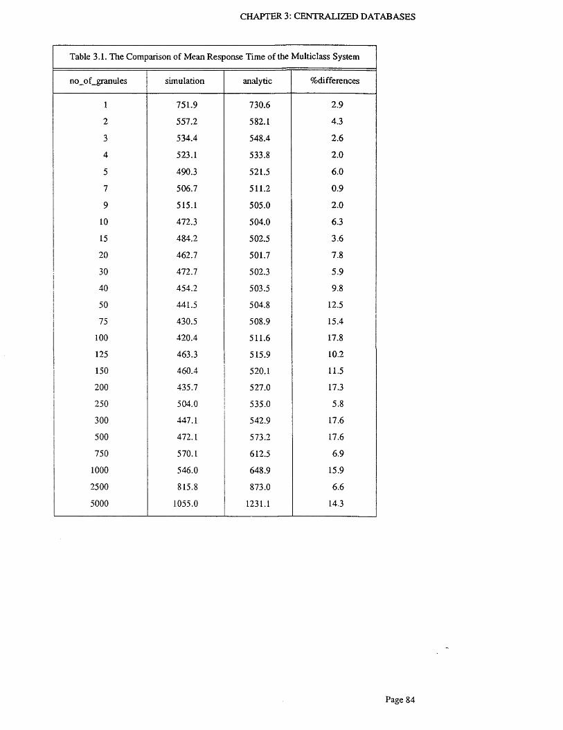
CHAPTER 3: CENTRALIZED DATABASES
Table 3.1. The Comparison of Mean Response Time of the Multiclass System
no_of_granules simulation analytic %differences
1 751.9 730.6 2.9
2 557.2 582.1 4.3
3 534.4 548.4 2.6
4 523.1 533.8 2.0
5 490.3 521.5 6.0
7 506.7 511.2 0.9
9 515.1 505.0 2.0
10 472.3 504.0 6.3
15 484.2 502.5 3.6
20 462.7 501.7 7.8
30 472.7 502.3 5.9
40 454.2 503.5 9.8
50 441.5 504.8 12.5
75 430.5 508.9 15.4
100 420.4 511.6 17.8
125 463.3 515.9 10.2
150 460.4 520.1 11.5
200 435.7 527.0 17.3
250 504.0 535.0 5.8
300 447.1 542.9 17.6
500 472.1 573.2 17.6
750 570.1 612.5 6.9
1000 546.0 648.9 15.9
2500 815.8 873.0 6.6
5000 1055.0 1231.1 14.3
Page 84

CHAPTER 3: CENTRALIZED DATABASES
Table 3.2. The Comparison of Useful I/O Time of the Multiclass System
no_of_granules simulation analytic %differences
1 7041.9 6618.4 6.4
2 8377.0 8264.2 1.4
3 9002.3 8772.3 2.6
4 9030.3 9023.5 0.1
5 9273.9 9249.8 0.3
7 9438.5 9463.2 0.3
9 9449.1 9601.2 1.6
10 9476.2 9623.5 1.5
15 9425.6 9669.6 2.5
20 9438.0 9698.6 2.7
30 9534.3 9693.9 1.6
40 9472.7 9675.7 2.1
50 9504.1 9652.3 1.5
75 9448.4 9577.8 1.4
100 9378.3 9528.7 1.6
125 9351.7 9450.0 1.0
150 9304.1 9371.8 0.7
200 9159.7 9248.5 1.0
250 9110.5 9107.9 0.0
300 8768.2 8971.7 2.3
500 8517.2 8489.3 0.3
750 7820.6 7933.8 1.4
1000 7359.8 7480.1 1.6
2500 4764.2 5530.7 13.9
5000 3408.6 3913.6 12.9
Page 85

CHAPTER 3: CENTRALIZED DATABASES
Table 3.3. The Comparison of Useful CPU Time of the Multiclass System
no_of_granules simulation analytic %differences
1 1759.9 1654.6 6.4
2 2091.9 2066.1 1.2
3 2237.4 2193.1 2.0
4 2258.9 2255.9 0.1
5 2304.9 2312.5 0.3
7 2309.9 2365.8 2.4
9 2337.4 2400.3 2.6
10 2324.9 2405.9 3.4
15 2358.4 2417.4 2.4
20 2354.9 2424.7 2.9
30 2377.5 2423.5 1.9
40 2354.9 2418.9 2.6
50 2339.9 2413.1 3.0
75 2332.5 2394.5 2.6
100 2324.9 2382.2 2.4
125 2316.5 2362.5 1.9
150 2280.0 2343.0 2.7
200 2260.0 2312.1 2.3
250 2250.0 2277.0 1.2
300 2177.5 2242.9 2.9
500 2097.5 2122.5 1.2
750 1920.0 1983.5 3.2
1000 1815.0 1870.0 2.9
2500 1190.0 1385.3 14.1
5000 825.0 978.4 15.7
Page 86
Chapter 4. Concurrency Control Model o f DDB
A distributed database system inherits most of the characteristics of centralized databases such as
locking, parallel transaction execution and multiprogramming. However some additional features o f
distributed databases, such as concurrency control and locking among distributed transactions, significantly
increase the complexity of the systems. In this chapter we aim to define an analytic model which can
represent the characteristics of the distributed database concurrency control and locking mechanisms. In a
distributed database system transactions are controlled by a concurrency control protocol to guarantee the
consistency and integrity of the system. The basic idea of a concurrency control protocol is to provide a
communication and control agreement between a coordinating process and a number of participating
processes. There is a wide variety of concurrency control protocols such as the basic two phase locking
(2PL), the primary copy 2PL, the majority consensus 2PL, centralized 2PL etc8,12. In this chapter we shall
first study the most well known two phase locking protocol, i.e. the basic 2PL. The other three 2PL
protocols will be studied in the next chapter.
Section 4.1 presents a formal specification of the basic 2PL and its communication structure. Section
4.2 introduces a novel method to systematically define a two phase commit protocol with access pattern
matrix, communication flow matrix, arrival rate matrix and Markov chain matrix. In section 4.3 a
distributed database locking model with fixed waiting collision resolution algorithm is introduced. Section
4.4 introduces an extended diffusion approximation method to model a distributed database with general
service time distributions. Section 4.5 extends the method introduced in chapter 3 to model the scheduled
waiting in a distributed database. Section 4.6 builds a simulation model for distributed databases and
validates the analytic model. In section 4.7 cases of performance results are analyzed and some useful
conclusions are drawn at the end.
4.1 System Specification
Locking is strongly associated with distributed databases as with centralized databases. In a two phase
locking protocol, transactions request locks in the growing phase before a common decision is reached; and
releases locks in the shrinking phase after the implementation of the decision8. The basic 2PL is to
explicitly detect and prevent conflicts between concurrent operations by implementing a growing phase for
transactions to obtain locks and a shrinking phase for transactions to release locks. Transactions, such as
Read. (X) for reading logical data item X and Write {X) for updating X, are issued from a transaction
manager TM. The physical copies of X, i.e. {x^, X 2 , ' ' ' , A'„,} ^ stored in local databases and
managed by database managers DMs. A TM always acts as a coordinator of a transaction; while a D M
as a participant. The basic 2PL protocol can be represented formally as follows:
Page 87
CHAPTER 4: DISTRIBUTED DATABASES
Basic 2PL Protocol:
Phase 1:
1.1 The coordinator TM* sends a P r e p a r e (X ) and lock request (PRE) message to all the participants
{DM,-, X e D M i ) .
1.2 Each D M i receives the message; and checks for the requested locks. If all locks are granted and it
is willing to commit, then it writes a transaction’s records in the log and sends a ready (RDY)
answer message to TM*. If it wants the transaction to be aborted, it sends an abort (ABT) message
to TM*.
Phase 2:
2.1 Upon receiving the answer message RDY or ABT from {DM,-, X e DM ,-}, T M * sends a commit
(CMT) message to all {D M ,-, X e D M i } if all o f them have voted RDY, otherwise it writes an
abort record and sends an ABT to all {DM,-, X e D M t }.
2.2 After receiving the command message from T M *, each D M i writes either a abort or commit
record in log; then executes the transaction and release the locks; and sends the acknowledge
(ACK) message to TM*.
2.3 TM* waits for ACK messages from all {DM,-, X e D M i } 1 t^ n writes a completion record in log.
Figure 4.1 show-s the communication structure for the basic 2PL. Two phases are shown in the figure.
During the first phase of the basic 2PL, locks are requested from all participants, which corresponds to the
growing phase. A decision about whether to commit or abort the transaction is made at the locked point.
Upon receiving commit, all participants will execute transactions and release locks in the shrink ing phase.
After the transaction is executed by all participants, the locks will be released, which is related to the
shrinking phase. The communication of a complete transaction need 4 ‘m messages, where m is the
number of participants involved.
4.2 Two Phase Commit Model Definition
The ultimate goal of this section is to define the Markov chain matrix of the queueing network model of
the distributed databases with two phase locking protocol. Here a systematic way to obtain the Markov
chain matrix is introduced. In section 4.2.1 the access pattern matrix, defined as the probabilities of node
access, is derived. Section 4.2.2 introduces a method to define the communication flow rates between
database nodes. Section 4.2.3 obtains the arrival rates of the queueing network from the communication
flow rate matrix. In section 4.2.4 the final Markov chain matrix is derived from the communication flow
rate matrix.
Page 88

CHAPTER 4: DISTRIBUTED DATABASES
source lock request locked point lock release sinkStage: 1 2 3 4 5
dm dmtm
dm tmdm . tm
RDY or ABTPRE ACKCMT or ABT
Phase 1 Phase 2
Figure 4.1. Communication Structure of 2PL
4.2.1 A ccess P attern iMatrix
In order to formally define the probability of node access, we introduce the concept of access pattern
matrix. It is denoted by
©11 co12 •
0)21 CO2 2 • ‘ K
a>/n (0K2 ' ‘ <&KK
where the element CO/y is the probability of a transaction accessing node D M j from node T M t and K is
the number of nodes in the system. The access pattern matrix is determined by the protocol, the read-write
ratio and the mean number of replicated copies. We shall first give a formal definition of the read and write
rules of the basic 2PL. The basic 2PL requires that write operations have to access all the copies of a
logical data item X while read operations need only to access one.
Definition 4.1: A Read (.X ) transaction generated at TM£ is governed by the following rules:
• If X eD M ^-, access
• If X e D M i-, access one o f the [ D M j , X e D M j } with probability 1 INf , where N f denotes the mean
number of replicated data copies in the system.
Page 89

CHAPTER 4: DISTRIBUTED DATABASES
where node A' is a local node and node j ( J ^ k ) is a remote node.
D efinition 4.2: A Write (X ) transaction generated at TMk is governed by the following rule:
• Access all of the {D M j , X e D M j }.
Let us denote N acCk as the mean number of database accesses generated by one transaction issued at
TM if.. According to the read and write rules, R ead(X ) accesses one data copy while Write (X ) accesses
an average of Nj- data copies. Thus we have
N acCk — Prob {R e a d } • 1 + Prob {W rite } -Nf
= (l-Y ™ »)+Y nv,W / (4.1)
in which ynVk is the read-write ratio given by
number o f write transactions generated at TM*7™, = -----------------:--------------- :---------------------- 3— — ---------- (4.2)
to ta l transactions generated at IM *
Suppose the total transactions generated by users at node k in one time unit are Xk- Thus the total number
of database accesses generated at TMk is given by
X/c — N acck Xk
X k k = l , " ' , K (4.3)
The access probabilities dependent on the read-write ratio Ynvt ^ mean number of replicated copies
N f . The probability of accessing a local data copy, i.e. from TMk to DMk , is given by
co^- = Prob [local access) k = l , . . . ,K
= Prob {Accesskk) k = l , . . . ,K (4.4a)
and the probability of remote access, i.e. from T M k 10 is
cokj - Prob { remote a c c e s s }
= Prob {Access^} k , j = l , . . . ,K an d j & k (4.4b)
The distributed function of the locations of data copies is given by Prob {X&DMk). Suppose the
replicated data copies are distributed in database nodes with a uniform distribution. The probability of a
data copy stored at DMk is given by
NfP r o b { X e D M k } = - 7 k = 1 K (4.5)
* K
The access probability can then be derived by the following theorems.
Page 90

CHAPTER 4: DISTRIBUTED DATABASES
T heorem 4.3: The probability o f accessing a local data copy from T M k is given by the access pattern
matrix w with
Ol
= , , L f ,------- k = l , . . . , K (4.6)
Proof: We shall first give the conditional probability of CO -.
% = Prob {Accesskk I X e D M k )Prob {X e D M k }
+ Prob {Accesskk \X e D M k }Prob [ X e D M k } (4.7)
where Prob {Accesskj \ X e D M k } denotes the probability o f access data copy at D M j from T M k
under the condition that there is a data copy stored at D M k • According to the read and write rules we have
Prob {AccesSkk\X * D M k ) = P r o b { R e a d ) l + P r o b { W r i t e ) lN acck
1
1 Yrvv* “*_ / Y rvi’k(4.8)
and
Hence
Prob {Accesskk 1X e D M k} = 0 (4.9)
N f N f1-— + 0 ( 1 — - )
K K^ k k ~
1 Yrwk
Nf_
K
Theorem 4.4: The probability of accessing a remote data copy from T M k ^ given by
N f / , N f s 1
(4.10)
Yrw't j y "K1 Yrn-t ) ( i )K f r ' K _ {cokj = -------------- ------------------------------------ k , j = 1 , . . . , K and j ^ k (4.11)
1 Yrw’* +Ay'Y/-H'Jt
Proof: The probability o f accessing a remote data copy from T M k IS determined by the conditional
probability of whether the copy is stored locally or remotely. That is
Page 91

CHAPTER 4: DISTRIBUTED DATABASES
cokj = Prob [Accessbj \X G D M kn X G D M j )Prob [X G D M kc \X G D M j }
+ Prob {A c c e s s ^ IX e D M k r S X e D M y-}Prob {X e D M k n X e D M j }
+ Prob [ A c c e s s kj IX e D M k r \ X e D M j } Prob {X e D M j }
+ Prob {A c c e s s k j IX e D M k n X e D M j } Prob {X e D M k r \ X e D M } }
The conditional probabilities about the locations of the data item X are given by
Prob { X e D M kn X e D M j } = Prob { X e D M k )Prob [ X g D M j \ X g D M k }N f N f —1
= ~K K - 1
Prob [ X g D M k r S X G D M j } = Prob [ X g D M k )Prob [ X g D M j \ X g D M k )
1—N f
~K
N,
K - 1
Prob [ X g D M k n X G D M ; } = Prob [ X G D M k \Prob {Xe D M ; \ X & D M k }
K1-
Nr 1
K - 1
Prob { X e D M k r S X G D M j} = Prob [ X g D M k }Prob {Xe D M j \ X e D M k
1 -N
K1 -
N fK
and the conditional access probabilities are given by
Prob [ A c c e s s k ; {X e D M k r \ X e D M : } =
Prob [ A c c e s s k ; | X e DM krSXG D M .} = ------------------------------;1 ”*Yn\’k
Prob [ A c c e s s k : \ X G D M k r X G D M :} = 0;
Prob [ A c c e s s kj \ X G D M k n X G D M j } = 0.
Substituting the above equations into equation (4.12), we have
(4.12)
(4.13a)
(4.13b)
(4.13c)
(4.13d)
(4.14a)
(4.14b)
(4.14c)
(4.14d)
Page 92

CHAPTER 4: DISTRIBUTED DATABASES
YrwkN f N j —1
K K - 1 (1 Yrwt ) A j " "Yrwk P i f K
N t
K - 1©*/
1 Yrw't+^/Ynv,.
X - I(4.15)
1 ~Ynvt +W/Y
Hence. []
4 .2 .2 C om m u n ica tion Flow M ethod
Here we introduce a novel method to represent the flow rate of transactions in the concurrency control
model. We shall use the concept of stages to define the two phase commit protocol. As indicated in figure
4.1, stage 1 is defined as the source point o f the system; stage 2 is the lock request point; stage 3 is the
locked point; stage 4 is the lock release or transaction execution point and stage 5 is the sink point of the
system. The communication flow matrix is to to define the flow rates of transaction from one stage to the
next. Suppose the distributed database system has K nodes. The communication flow matrix from stage s
to stage ^ -f-1 is denoted by A.s with element a t y representing the flow rates o f messages from node i to j .
Between the first and the second stage of the two phase commit protocol, a PRE message generated at
T M i has to be sent to [ D M j , X G D M j } with the flow rates given by
a \ f = Xi (£>ij ( i , j = K ) (4 .16)
where A.,- is the transaction arrival rate at T M \ . The communication flow matrix at stage 1 can be obtained
by
A j C O n A q c o ^ • • •
A<2 0l>2 i Xi 0>22 ’ ' ' A-2 Cl>2kA, = X^ X K w =
XK (£>K l X f( co^ 2 X k &k k
(4.17)
Between stage 2 and 3, all DMs received PRE message will send back either a CMT or ABT message
back to TMt. This is a reversion o f the transmission procedure between stage 1 and 2. Its communication
flow matrix A2 can be obtained simply by transposing the matrix A y. That is
A2 CO21 * • • A/fCO^]
A,[Cl>12 A2 CO22
A2 = A [ =
Xy to y z X 2 (PhfC
(4.19)
Page 93

CHAPTER 4: DISTRIBUTED DATABASES
Stage 3—4 and 4—5 are respectively the same as stage 1—2 and 2—3. Their communication flow
matrices are given by
and
A 3 - Ay;
Aa = A'
(4.20)
(4.21)
4 .2 .3 A rriva l Rate M atrix
The communication flow matrix introduced above can be used to calculate the arrival rate at various
service centres very efficiently. The arrival rate at stage s is defined by a vector with K members
(4.22)
where X is the arrival rate of the node k at stage S.
At the source stage, i.e. s = 1 , the arrival rate at node k is given by Xk . That is
X{l ) = X k k = l , . . . , K
A, = X[l) x p • • • x p XK
(4.23)
(4.24)
At the lock request stage, i.e. S = 2, the arrival rates of lock request service centres can be obtained by
A? = Vr A, (4.25)
where
v = (4.26)
is a vector o f K elements with all elements equal to I. Thus
Page 94

CHAPTER 4: DISTRIBUTED DATABASES
A, = 1 1
^ c o n ^ i ( o 12
A,2G>21 ^ '2(022 ' ’ '
XK <tiK y ^ K ^ K l ^ K ^ K K
(4.27)
A,iC0ii+A«2032L+ * ' ' 1 ^1® 12'+'^ 2 C022+ * ’ ' _,_ 'A:coa:2 ^ l C0l/i:+ ^ 2 (02/i:+ ■ ■ ' + ^ K ^ K K
Similarly the arrival rate vector at locked stage, lock request stage and sink stage are respectively given
by
A 3 = VtA 2 ; (4.28)
A4 = Vt A 3 ; (4.29)
and
A5 = Vr A4 (4.30)
The general formula to obtain the arrival rate at various service stages is given by
A s = V TA s _ l 5=2, . . . ,5 (4.31)
It should be noted that the communication channel from node i to j has been used for four times during
four stages of the two phase commit protocol. The overall arrival rates of the communication channels
should be equal to the sum of the arrival rates at these four stages. If we use Ac to denote the
communication flow rate matrix, A c is equal to the sum of the flow rates matrices at four stage. That is
4A r = £ A , (4.32)
5 —1
It is a K x K dimensional matrix with element X t y being defined as the arrival rate of communication
channel from node i to j .
4 .2 .4 M ark ov Chain M atrix
The Markov chain matrix is an essential factor in defining queueing network models. When a system is
as complicated as a distributed database, to obtain the Markov chain matrix of the system is not a
straightforward task. This is especially true when the system with several stages has to share
communication channels. A systematic way to solve this problem is to use our communication flow method
to obtain the Markov chain matrix.
Page 95

CHAPTER 4: DISTRIBUTED DATABASES
Let us first introduce the concept of the local Markov chain matrices. Let denote the matrix of the
input flow to the communication channel at node k and the output flow from the communication
channel at node k. In P ^ matrix, the element p si ( 5 = 1 , . . . ,5 ) (/= 1 ,...,A T ) denotes the probability of a
job entering the i th communication channel in node k from stage 5. We have
I i A i
p ^ > =
I i A t l
* 2 ^ 2
I2A2 |
I3A3
I3 A 3 I
I4A4
I4A4
I5A 5
(4.33)
I 5 A 5 I
where 1^ is a vector with k th element equal to one and the rest equal to zero, i.e.
I/ =
Since there is no traffic flowing from stage 5, i.e. the sink, to the communication channels, we have
A 5 = 0
(4.34)
(4.35)
The overall input matrix is equal to
P i =
'p j l ) 0 0 “
0 p } 2) • 0
0 0 . . p f )
(4.36)
Let us denote P q as the output Markov chain matrix defining the traffic from communication channels
to the service centre at various stages. The element p j s o f P q is defined as the probability of traffic from
the /th communication channel to the service centre at stage 5. And we further define matrix P£jP in
which its element p * $ is the probability of traffic from from the ith communication channel at node k to
the 5th stage. We have
Page 96

CHAPTER 4: DISTRIBUTED DATABASES
P ^ =l o A o l J I 2 A 2 I 2 I 3 A 3 I 3 I 4 A 4 I 4
Io A c Io I i A c I j \ 2 A c \ 2 I 3 A C I3 I 4 A c I 4
0 0 0 0 0
(4.37)
Since there is no traffic flowing from the communication channels to the source stage, we have
Ao = 0
The overall output Markov chain matrix P q is given by
(4.38)
> b l) pb2) •. . p<K)
p y > pb2) ■ . . P ^ >
p 9* p g ’ • . . p 0 D
(4.39)
Combine the input and the output Markov chain matrices together, we can obtain the overall Markov chain
matrix of the queueing network model.
P; 0
0 P0P = (4.40)
In this section, we have introduced an systematic method to define a distributed database in the form of
communication flow matrix, access pattern matrix, arrival rate matrix and Markov chain matrix, which has
not been addressed before. Previous researches can only pass the problem of defining a complicated
distributed database to individual users, who have to manually define a model. This tedious task can be
avoided by using the systematic model definition method introcuded in this section.
4.2 .5 Q ueu ein g N etw ork M odel
Using the result derived in the previous sections, a distributed database can be easily defined as a
network of queues with the defined Markov chain matrix, as shown in figure 4.2. It illustrates the kxh node
of a distributed database consisting of K + 2 service centres. Let us denote service centres { k i , i = l , . . . , K }
as the communication channels with the arrival rates defined by equation (4.32) and service centres k ^ +
and k fr +2 as the lock request centre at stage 2 and the transaction execution centre at stage 4 respectively.
The probability of a transaction going from one service centre to another is uniquely defined by the Markovi
chain matrix in equation (4.40).
Page 97

CHAPTER 4: DISTRIBUTED DATABASES
Node k
to Node 1
to Node &+1
from Node 1
to Node Kfrom Node k + l
from Node K
Figure 4.2. 2PL Distributed Database Model at Node k
4.3 Fixed Waiting Model
4.3.1 L ock in g M odel with F ixed W aiting
Let us first discuss the fixed waiting scheduling algorithm. At the lock request stage, i.e. stage 2 in
figure 4.1, a transaction first requests for locks at a DM with a preemptive priority. The database manager
then chedksthe lock table for each required lock; which means that if m locks are required, the database
manager will check the locks table for m times. If all the locks are granted, the transaction will leave the
DM; otherwise the transaction is said to be blocked and must enter a blocked queue. The transaction will
wait in the blocked queue for a fixed amount of time and then request those locks again until it grants all o f
them. All the locks will be released at the lock’ release stage, i.e. stage 4, after the transaction is executed.
The fixed waiting scheduling algorithm can be best modeled by a network o f queues as shown in figure 4.2.
Page 98
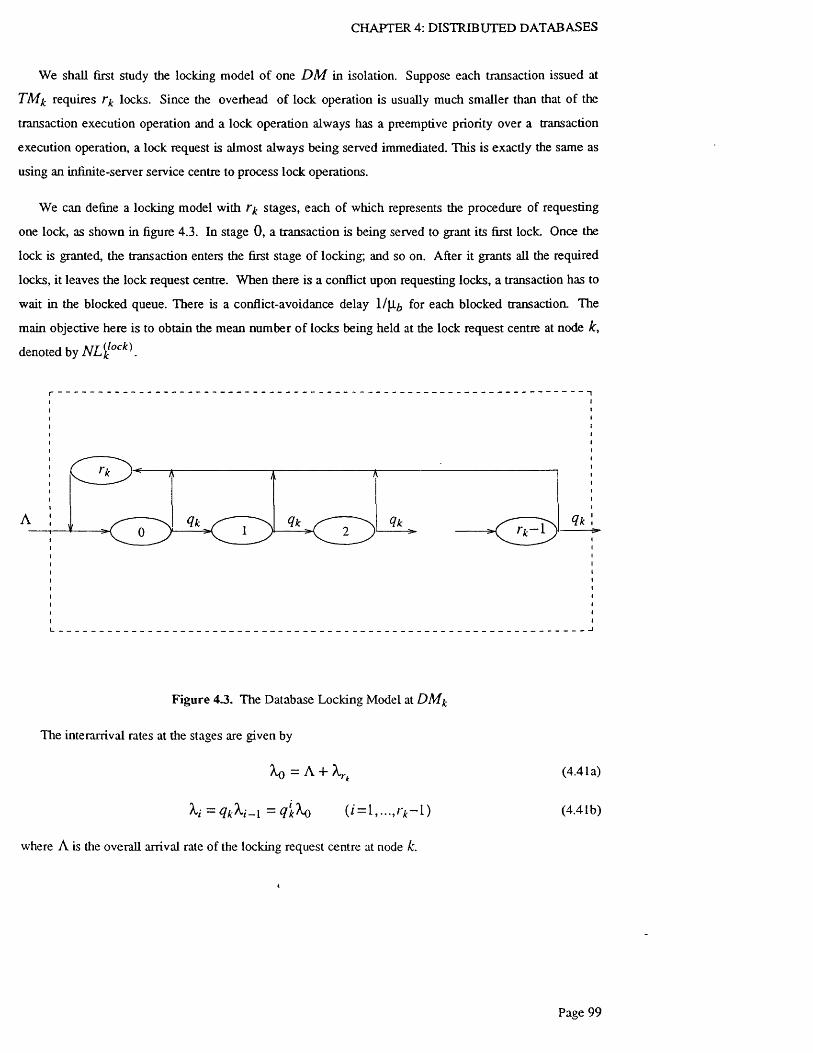
CHAPTER 4: DISTRIBUTED DATABASES
We shall first study the locking model o f one D M in isolation. Suppose each transaction issued at
TMfr requires locks. Since the overhead of lock operation is usually much smaller than that of the
transaction execution operation and a lock operation always has a preemptive priority over a transaction
execution operation, a lock request is almost always being served immediated. This is exactly the same as
using an infinite-server service centre to process lock operations.
We can define a locking model with r£ stages, each of which represents the procedure of requesting
one lock, as shown in figure 4.3. In stage 0, a transaction is being served to grant its first lock. Once the
lock is granted, the transaction enters the first stage of locking; and so on. After it grants all the required
locks, it leaves the lock request centre. When there is a conflict upon requesting locks, a transaction has to
wait in the blocked queue. There is a conflict-avoidance delay 1/|I/, for each blocked transaction. The
main objective here is to obtain the mean number o f locks being held at the lock request centre at node k,
denoted by N L <i ° ck).
I----------------------------------------------------------------------------------------------------------------------------------------- 1
F igure 4.3. The Database Locking Model at DM *
The interarrival rates at the stages are given by
Xo = A + Xri (4.4 la)
h = q k h - l r* -L ) (4.41b)
where A is the overall arrival rate of the locking request centre at node k.
Page 99

CHAPTER 4: DISTRIBUTED DATABASES
r k- 1
t= 0
r*_1
z=0
= < l - ^ ? ) A o (4.41c)
The above equations can be rewritten as
X o = Ar * - l
j=Q
= q r*A (4.42a)
X1 = q tk rkA (4.42b)
and
r*-lA I (1 - q t )q{
Xr, = = (?r*-D A (4.42c)
)=o
Applying open queueing network theory32 we can obtain a product form solution,
P 0{n0) P l ( n l ) • • • Prt(nrt)P ( n 0, n u - • * ,nr ) = --------------------- (4.43)
O
where P (hq n i , • • • ,nrt) is the steady-state probability of a network state with a>+1 service centres,
Pj(rij) (j=Q,. . . ,rk) is a factor corresponding to the steady-state probability of the state of service centre
j in isolation and G is the normalizing factor given by
G - I = Prob {n 0= 0 }Prob {n i = 0 } • • • Prob {nrk =0} (4.44)
The steady-state probability of the state of service centre j in isolation is
Pj(n) = ——-— Prob {n =0} (4.45)
n ^ - ( o7=1
where 14/(0 is the service rate at service centre j where i customers are being served. For infinite-server
service centres
Page 100

CHAPTER 4: DISTRIBUTED DATABASES
M O = %■ (4.46)
Thus P;(n ) becomes
V ,n
mi = 1
^ 7
J _ Mn ! A
Prob {/i =0} (4.47)
Substituting equations (4.44) and (4.45) into equation (4.43), we have
P i n )i ^0
- J^1
n \1
\ K ]\X) « l ! M-ik. J » r ,I
X*0 A ] n \ V
(«0+«i+' '' +«r4)! Ho A .(no+n i + * * • +nr )\
Xq A.!— + — +
l^o Hd
rt0 ! « i ! • ' ’ « r t ! ( n 0+ / i , + • • • +n )
(n 0+n • +nr )\
Let n = Hq + n i + • ■ • + nr , we have
P (n ) =
i —
n !
(4.48)
(4.49)
In the locking model, l / | l t ( /= 0 , . . . ,r* — 1) is equal to the mean service time spend in lock scheduling at
jth stage of locking. Since the lock request sendee times at all stages are equal,
\li = \ls ( / = 0 , * • • ,rk- 1) (4.50)
where ^ is the service rate for requesting one lock. Substituting equations (4.42a-c) and (4.50) into
equation (4.48), we have
Page 101

CHAPTER 4: DISTRIBUTED DATABASES
P (n ) =
rk- 1 nlr r*
£ > Hi-A +
~rk iA
\^ag(4.51)
n !
We can easily conclude, from the above result, that the locking model with r £ stages can be aggregated
into one infinite-server service centre with its mean service time l / | l a^ equal to
1
^a g ( 1 - ^ ? ) |1 ,
where 1/jXj, is the service time of the blocked queue.
si 1 si r,c 1<lk ” 1(4.52)
As given by equation (3.40), the waiting in the blocked queue with fixed waiting approximately equals
to the time of two successive completions of transaction executions. That is whenever a transaction
completes, the blocked transaction restarts. Since the throughput of transaction execution centre is A,£+2 ,
we have
_L_
\Lb
1
VK+2
Now let us calculate the mean number of locks held at the aggregated locking request service centre at
model k, which is defined as
rkNL]lock) = ]T(77z£ number o f locks held a t stage i by each customer)-
i=1
{The number o f customers a t stage i ) (4.53)
According to the definition of the locking model, a transaction having granted i locks will enter stage i.
Thus the number of locks held at stage i by each transaction is equal to /. And the mean number of
transactions at stage i can be easily calculated by applying to the open queueing network theory for
infinite-server service centres. That is
_ X,nt — — ( / = 0 r * ) (4.54)
M;,
Thus we have
Page 102

CHAPTER 4: DISTRIBUTED DATABASES
source lock request locked point lock release sinkStage: 1 2 3 4 5
/ S > \
-------
-------
PRE R D Y orA B T CMT or ABT ACK
locking and blocking execution
Phase 1 Phase 2
F igure 4.4. Distributed Database Locking Model
f tNL.$ock) =
i = 1
'W zXf-
r*-l
r*-l
. / —r t A
= I (4-55)'= i q k V *
The method of evaluating locking by using inlinite-server queueing network has not been used before.
Tay, Suri and Goodman, who introduced a flow diagranvnethod to evaluate locking in centralized database,
ad m itted that the method is controversial and they can offer no theoretical justification for it78,77. By
applying our method to their locking model of centralized database, we can obtain exactly the same result
under the assumption of exponential service time distribution. Moreover we can easily and consistently
extend this method to distributed locking.
Page 103
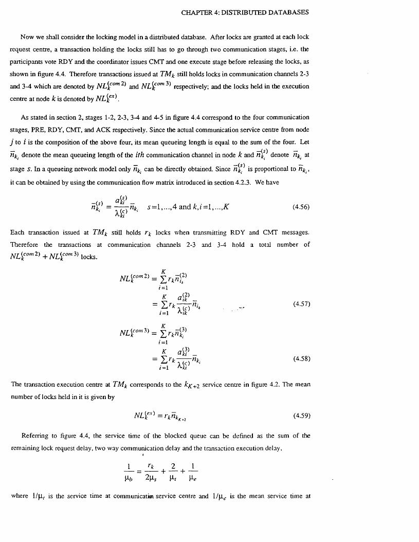
CHAPTER 4: DISTRIBUTED DATABASES
Now we shall consider the locking model in a distributed database. After locks are granted at each lock
request centre, a transaction holding the locks still has to go through two communication stages, i.e. the
participants vote RD Y and the coordinator issues CMT and one execute stage before releasing the locks, as
shown in figure 4.4. Therefore transactions issued at T M k still holds locks in communication channels 2-3
and 3-4 which are denoted by N L ^ om and N L ^ om ^ respectively; and the locks held in the execution
centre at node k is denoted by N L ^ X^.
As stated in section 2, stages 1-2, 2-3, 3-4 and 4-5 in figure 4.4 correspond to the four communication
stages, PRE, RDY, CMT, and ACK respectively. Since the actual communication service centre from node
j to i is the composition of the above four, its mean queueing length is equal to the sum of the four. Let
nk. denote the mean queueing length of the ith communication channel in node k and denote nkj at— —(5 ) —
stage S. In a queueing network model only nk can be directly obtained. Since n k. is proportional to nkj,
it can be obtained by using the communication flow matrix introduced in section 4.2.3. We have
= - ■ * n k . 5 = 1 , . . . ,4 a n d fc, K (4.56)^ki
Each transaction issued at T M k still holds r k locks when transmitting RDY and CMT messages.
Therefore the transactions at communication channels 2-3 and 3-4 hold a total number ofN L <g°m2) + N L (^oml) lockj
NL<f°m2) =
a f t -= T , r k - — ni (4.57)Z-r * » (C) lk ■
i =I A'lk
N L S T " 3' =
K a [ f _= ( « 8)
/'= 1 Kl
The transaction execution centre at T M k corresponds to the k%;+ 2 service centre in figure 4.2. The mean
number of locks held in it is given by
N L [ eA) = (4.59)
Referring to figure 4.4, the service time of the blocked queue can be defined as the sum of the
remaining lock request delay, two way communication delay and the transaction execution delay,
J ^ + J2_ + J _
M-6 \k-t \ke
where 1/ji, is the service time at communication service centre and l/j_Lc, is the mean service time at

CHAPTER 4: DISTRIBUTED DATABASES
transaction execution service centre.
Another very important parameter to describe the locking model is the probability of conflicts at D M
defined as
mean number o f lock requests at node k i~qic = ---------------------------------------------------------------------
number o f granules at node k NL^ock) + N L i com2) + N L [ com3) + N L [ ex)
= Lk
where N L ^ ock\ N L ^ om2\ N L <f om^ and N l J f ^ are the number of locks being held at lock request,
RDY, CM T and execution stages respectively. Substituting (4.55), (4.57), (4.58) and (4.59) into the above
equation, we have
i - q k =Q.k l — 1
Y j in k + r kaf t '1 - a i f _
+ 'n k.«=1 " A # '
+ nJk +i
(4.60)
This result is very important in the derivation of the whole distributed database model, q^ is dependent
on almost all the parameters of the system, because in distributed locking lock conflict rate is related to the
distribution and granularity of locks, number of transactions holding locks and the operatins of locks. On
the other hand, other parameters also depend on q £. Once q^ is obtained, they can also be easily
calculated, q^ can be calculated by solve the equations iteratively with numerical method.
4.3.2 Q u e u e in g N e tw o r k Solut ion
The queueing network model of the distributed database system with the basic 2PL is shown in figure
4.2. Each node is represented as one chain with connections to other chains. Any two nodes
communicating with each other through a data communication channel represented as a single server
service centre. The locking request is presented as a single aggregated service centre. Transaction
execution service centre is served by a cpu-i/o compound server as discussed in section 2.5. The whole
distributed database constructs an open queueing network with transactions arriving at the source and
departuring at the sink.
We shall first present the queueing network solution of a distributed database system with exponential
service times. Applying Jackson’s queueing network theory, the open system has a product form solution
of
P l ( n i ) P 2 ( " 2 ) • ~ • PniOhn)
G(4.61)
where m is the total number of service centres in the system, P ( n i ,n 2 , ' ’ * , tlm ) is the steady state
probability of a network state, P j { n j ) , j = i , . . . , m ) is a factor of the steady-state probability of the state o f

CHAPTER 4: DISTRIBUTED DATABASES
service centre j in isolation, and G is a normalizing constant.
The M aikov chain matrix of the open queueing network of the distributed database is given by equation
(4.40) and its arrival rate matrix is given by equation (4.32). We shall define
P j =h tMy
(4.62)
as the throughput of service centre j , where 1/jXj is the mean service time of service centre j . Applying
Jackson’s theory, the system utility for single server service centre is
and for infinite-service centre is
*0 = Py
U j = 0
(4.63a)
(4.63b)
The mean queueing length for single server service centre is
PjU ; =' 1 -P ;
(4.64a)
and for infinite-server service centre is
n j ~ (4.64b)
Applying Little’s law the mean response time of service centre j is
7F;R j = ~*r~ (4.65)
Ki
4.4 Extended Diffusion Approximation Approach
4.4.1 Diffus ion A pproxim ation Solution
In most performance evaluation models, interarrival process is assumed to be Poisson and service time
be exponentially distributed81,29,73. However in a real world service time distributions do not usually fall
into this category. For instance the service time distributions of computer system tend to be
hyperexponential54,55. Diffusion approximation26,39,37 method provides a solution to the nonexponential
queueing network problem.
For general queueing networks with single server service centres, a diffusion approximation model was
first introduced by Gelenbe and Kobayashi26’39. The model can be used in a wide range of applications.
The method can be applied to the queueing network with only single server service centres. Since the
locking in a distributed database is modeled by an infinite-server service centre, the restriction on single
Page 106

CHAPTER 4: DISTRIBUTED DATABASES
server service centre needs to be released. We shall first present the conventional diffusion approximation
method and then further extend it to the queueing networks with infinite-server service centres.
We shall consider an open queueing network as in the previous section. Let ek be the relative
throughput at service centre /,
me-i = P o i + ' Z e jPji (z = l , . . . ,m ) (4.67)
7=1
where m is the total number of service centres in the open distributed database queueing network and p i j
is the element of the Markov chain matrix given in equation (4.40). The arrival rate of service centre i is
proportional to the relative throughput.
Xi = V ; (4.68)
The utilization of the service centre i is
Ao e ipi = , i f A o ^ M i ( / = l , . . . , m ) (4.69)
\ l i . . - •'
Under the condition of heavy traffic, the total number of arrivals to station / in the interval [0 ,f ] will
be normally distributed with mean
V (4.70a)
and variance
m£ [ ( C j - ^ p j i + ^ X j P j i t (i = l , . . . , m ) (4.70b)
j=0
where C j is the squared coefficient o f the variation of the interarrival time at service centre j . In the
equation we have used the fact that the sum of independent normal random variables is normally
distributed with variance being the sum of individual variances.
We can now construct the diffusion approximation to the length of an individual queue. We have
9 / i l V i . f ) 0 d f i ( X i , t ) i d 2 f i ( X i , t ) , „ , —— p, - + — cq — - 4- Xi P oi ( t ) S ( X i~ 1) - 0 (4.71)
d t dXi 2 f a t
d 1 d f i ( X i , t )— P o i ( t ) = - h P o i ( 0 + L i m + — o q r ] (4.72)d t .v ,—>o* 2 dXi
f i ( 0 , t ) = 0 (absorbing boundary) (/ = l , . . . ,m ) (4.73)
where f i ( X i , t ) is the density function approximating the length of the i th queue, P o i ( t ) is the probability
of the i th queue being empty, and 5 (a , —L) is the Dirac density function concentrated at Xi—1. The other
Page 107

CHAPTER 4: DISTRIBUTED DATABASES
parameters of the above equations are given by,
P i = A, — [Xr-
Pi 'i^Mi
mcq = Pi\i iK} 4- £ [(Cj - l ) p j ; + l ] \ j P j i
y=o
X C i - l ) -X( 4" XiP ii (1 p t-)
X (Cj-DXjpji
(4.74)
(4.75)
(4.76)
0 = 1 , . . . ,m ) (4.77)
where is the squared coefficient o f variation o f the service time distribution at service centre i.
Ci 0 = 1, .. . ,m ) can be easily solved by numerical methods.
The stationary solution of equations (4.71), (4.72) and (4.73) is
A i > l
where
p j ( e u - l ) e
p , - ( l - e YiJr'). 0< v ,< l
Pot = 1 - p ,
Yi = - 2 p , / a ;
P/ = V P i
The approximate average queue length is
= P i 1 -2 P/
If for some i, p a ^ O , we have to modify the parameters of the /-th queue so that
(i) p i j ( j = 1 ,... , m 4-1) is replaced by
0Pij = i
P i j
G -P u)
if 7=1
if y * i
2(ii) jl, and K t are replaced by
(4.78)
(4.79)
(4.80)
(4.81)
(4.82)
(4.83)
^ = p , ( i - P i i ) (4.84a)
Page 108

CHAPTER 4: DISTRIBUTED DATABASES
K f = a - P i i ) K f + p ii (4.84b)
respectively.
Applying Little’s law, the average turn-around time o f the system is given by
« HiT a = Z T - (4 '85)
1=1*0
4.4.2 Diffus ion A p pro x im a t io n So lu t ion o f Distr ibuted L ock ing
The above diffusion approximation queueing network method is suitable only for single server service
centres. But there are some infinite-server service centres in our model. We shall now further extend the
method to infinite-server service centres, i.e. I G I G /«*> queue.
Now let us first study the G f M I«*> queue, without lossing the generality of the problem. Consider that
customers arrive at epochs T j , T2 ,... and assume that the interarrival time T*-+ i —'Xk (k = 0 , 1,...; To= 0 ) is
i.i.d. with common distribution function G ( t ) = P {xk+i~Xk< t } (k= 0 ,1 , . . . ) and mean interarrival time
t. Also assume that the service time is exponentially distributed with mean x. Let be the number of
customers in the system prior to the interarrival o f the ith customer
p i X k + i = j } = & { X k + i = j \ X k = i \ P { X k = i \ ( 4 . 8 6 )i=0
The transition probabilities are
P i j = p { l k + \ = j \ X k = i I (4-87>
The unique stationary distribution is
Y l j = L i m P [ %k = j ) ( J = Q , 1 , . . . ) ( 4 . 8 8 )k —t°°
After taking the limits on both sides o f equation (4.86), its stationary distribution becomes
OO
n y = Z P i j U i O ' = 0 , 1, . . . ) ( 4 . 8 9 )i =0
together with the nomialization equation
OO
X n y = i (4.90)j = 0
where ‘
p 0 = 0 ( (+ 1 < 7 < 0 ) (4.91)
At the (A' + l )th arrival, there are approximately N servers being continuously busy during interarrival time

CHAPTER 4: DISTRIBUTED DATABASES
Xk+i—'Xk . Since the service time of each server is assumed to be exponentially distributed with mean JC, it
yields that
p (x * + i= j lx t= ' .'ci + i - ' ci-=M = ( i + i - ; > 0 ) (4.92)( i + l - y ) !
and since the interarrival time has distribution function G ( /) , we have
p , j = f (^ l. ,XJ +' J e ■' d G ( t ) ( i + l - / > 0 ) (4.93)
Substituting (4.93) into (4.94), we obtain
(4.94)1 o 0+1-7)!
With a change of variable, this equation becomes
n y = £ n i t M f tE lliL e-N"x dG{t) _ ( 4 9 5 )/=0 0 1.
If Fly is replaced by
n ; = A o y (4.96)
equation (4.95) becomes
A o y = Y Aco ' +y_1 f W t ' D Le-M'* d G ( t ) J o i !=o
co = f J o
= G ( ( 1—CO) N / x ) (4.97)
where G (s) is the Laplace transformation of G { t ).
Let
a=(l-co )A 7x (4.98)
Applying this equation to (4.97), we obtain
l - - ^ = G * (c t) (4.99)N
If we expand G (oc) in a power series, it becomes
Page 110

CHAPTER 4: DISTRIBUTED DATABASES
1 ~ = 1 - t a + f -a - + o ( a 2 ) (4.100)N 21
For the system in equilibrium, L i m G ( t ) corresponds to L i m G ( a ) . Thus the higher order terms of CCt —>oo a —>0
may be neglected. The above equation therefore becomes
a . M z E L B X (4.101)t 2
For the G / G / ° ° system in equilibrium64, the average number of busy servers tends to be the traffic /
intensity p .
p = x f t ^ N (4.102)
Thus we have
From this equation, t 2 becomes
{xfPf ~ N 2 (4.103)
1 9 —2t L = G t + t
~ < y l + (x / N ) 2 (4.104)
Because of the exponential nature of the service centre.
o l = x 2 (4.105)
t 2 ~ g 2 + a l l N 2 (4.106)
Thus equation (4.104) can be written as
Applying (4.106) to (4.101),
I (4 .107)C a + o l / N
Compare this equation with the G I G / I result under heavy traffic approximation given by
27y-v?/_£) (4 l0g)
v i + O b
we can conclude that the G I G l°° can be replaced by the G I G /1 with service capacity equal to xl N.
Finally we shall obtain the mean number of busy servers N. The mean waiting time of the G / G / l
service centre with service capacity xIN under heavy traffic assumption is equal to35

CHAPTER 4: DISTRIBUTED DATABASES
I o l + t 2W = — = -------------- 3 “ (4.109)
a 2 ( t - x / N )
Applying Little’s law, the mean queueing length, i.e. the mean number of busy servers here, is given by
- W N = —
csl + t 2
27(7—x/ N)
From this equation, the number of mean busy servers can be obtained as
(4.110)
N = L ( g J / t + 2 x / t + l )
Since t — and x = 1/Ll,
N = ^ - ( k 2o l + 2 X / 1 1 + 1 ) (4.111)
The above result extends the diffusion approximation method to infinite-server service centers. Prior to
this, diffusion approximation method can only be used to model single-server queuing networks. By
applying to the above extended diffusion approximation method, we can model both single-server and
infinite-server queueing netowrks with non-exponential serivice times. The method can be used to model
not only distributed databases but also general queueing networks of computer systems.
With the above extended diffusion approximation method, we are now able to treat the lock request
service centre in the same way as other single server service centres. The lock request service centre j g + i
in figure 4.4 is an infinite-server service centre which can be represented by a single server service centre
with service capacity equal to |ly AT). The throughput of lock request service centre
jfC+l is defined as
p * . , = ■ = ------------- <4-112>Jk+1
where N is given by equation (4 .111) and can be rewritten as
1 2X;rr 1 , -v ? jk+i , .N ■. = — (Xi a , H---------------h i )7 / f + i o J * - ' - ' ' K + 1 I I .
rjic+i
1 ^ A > i
■ t < c « ■ + "
Page 112

CHAPTER 4: DISTRIBUTED DATABASES
Heie C iK» is the squared coefficient o f the variation of the interarrival time at service centre Jk +i » which
is equal to the sum of the independent variance of the interdeparture time of all the other service centres to
centre j K + l.
1 mC j K+l = T S t ( C i ~ ^ P i j K+i + * ^Pi jic+i (4.114)
jfC+\ i = 0
The probability of the locking conflict can now be solved by
The mean throughput of the lock request centre , the squared coefficient C {-, and the mean queueing
length rii ( i = l , . . . ,m ;£ = 1 , . . . ,K ) can be respectively obtained from equation (4.112), (4.77) and (4.82).
In this section, we have introduced an extended diffusion approximation method to model distributed
database systems with non-exponential service times. Previous researches can only model d istribu ted
databases with exponential service time. By applying the extended diffusion approximation method, we
can model non-Poisson interarrival process and non-exponential service time distribution. M oreover
locking and transaction blocking are also modeled by using the phase method. Various characteristics o f a
distributed database, such as data replication, data locality, read-write ratio, lock granularity, etc. are
factored in. Using our method, a distributed database can therefore be modeled in a systematic way, which
is not available before. The model can achieve a high degree of accuracy because of the introduction of
the extended diffusion approximation method and enclosure of all the important characteristics o f a
distributed database.
4 . 5 V a l i d a t i o n b y S i m u l a t i o n
4.5.1 S im ulat ion M o d e l
In order the verify the analytic model introduced in the previous sections, a simulation model of basic
2PL with fixed waiting collision resolution algorithm is built as shown in figure 4.5. The model simulates
an open distributed database system with transactions entering and leaving the system at a steady rate. A
transaction goes through several stages (i.e. PRE, lock, RDY, CMT, execution and ACK) in the system.
The coordinator starts with dispatching a transaction into several sub-transactions (sending PRE), which go
to the communication queues to reach a remote destination. The dispatched sub-transactions then enter the
lock queue to request locks. Upon conflict, they wait a fixed period and restart again; otherwise they send
RDY to the coordinator through the correspondent communication channel. When the coordinator collects
all the RDY answers from the participants, it reaches a commit stage and a CMT message is dispatched and
sent to the participants through the communication channels. After receiving the CMT message a
Page 113
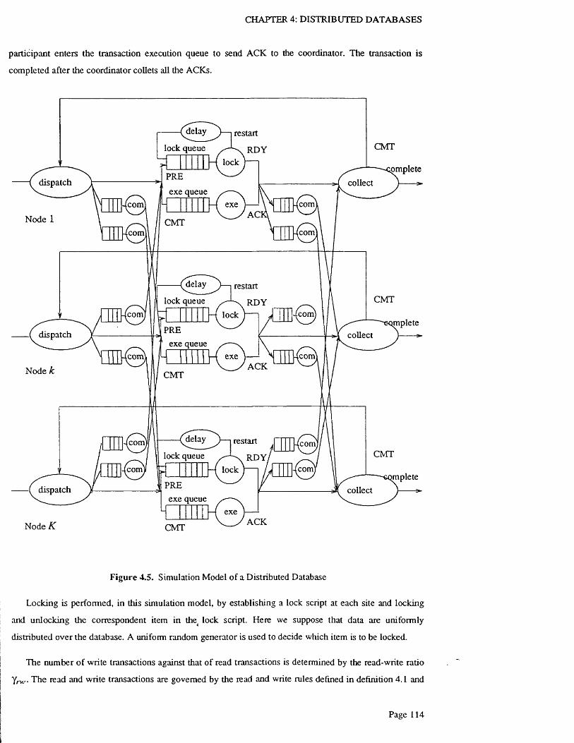
CHAPTER 4: DISTRIBUTED DATABASES
participant enters the transaction execution queue to send ACK to the coordinator. The transaction is
completed after the coordinator collets all the ACKs.
(delay
lock queue
restartCMTRDY
lockcomplete
PREdispatch collect
exe queuecomexecom
A CNode 1 CMTcomcom
(delay
lock queue
restartCMTRDY
lock -{comcommplete
PREdispatch collectexe queue
comcom exeACKNode k CMT
(delay
lock queue
restartcom com,CMTRDY,
lock comcomm plete
PREdispatch collectexe queue
exeACKNode K CMT
F igure 4.5. Simulation Model o f a Distributed Database
Locking is performed, in this simulation model, by establishing a lock script at each site and locking
and unlocking the correspondent item in tire lock script. Here we suppose that data are uniformly
distributed over the database. A uniform random generator is used to decide which item is to be locked.
The number of write transactions against that of read transactions is determined by the read-write ratio
yw . The read and write transactions are governed by the read and write rules defined in definition 4.1 and

CHAPTER 4: DISTRIBUTED DATABASES
4.2 respectively.
In the simulation model there are four types o f queues, the communication queue, the transaction
execution queue, the lock queue and the delay queue. The service time demands of the above queueing
centres have general distributions. The actual service time distribution functions used in modeling the
above queues can be determined by measurements from a real system. The measurement method to obtain
the service time distribution functions can be found in appendix C. Since the main purpose of this section is
to validate the analytic model by simulation, it is not important as to which distribution function is chosen.
For simplicity, a constant service time for com m unication' is used since a packet switching network tends
to have a deterministic packet transmission time37. An exponentially distributed service demand with
single server for transaction execution is used in this example and an exponential service time with
infinite-server for locking and blocking delay are used.
4.5 .2 C o m p a r iso n o f Results
As an application of the model, the test system consists o f five database nodes. Without losing
generality, the network of the test system is assumed to be fully connected. The parameters of the model
are set as follows,
• mean service rates and squared coefficients of variance
Table 4.1. The service time parameters of figure 4.6 to 4.11
Service centre Me an service rate (1 I s ) Squared coefficient o f variance K
Data transfer channel 18.182 0
Lock request scheduling 1160.09 1
Transaction execution 8.0 1
The interarrival service time is supposed to be exponentially distributed with
Xjj = l (4.115)
• Other parameters
Page 115

CHAPTER 4: DISTRIBUTED DATABASES
Table 4.2. The parameters of figure 4.6 to 4.11
Specification Value
Number of database nodes k 5
Interarrival rate X q ( I I s ) 0-10
Update ratio y ^ 0.25
Number of duplicated copies N f 5
Number of locks requeried r 15
Number of granulars L 1500
In order to verify our analytic model and compare it with other models, three groups of results are
obtained based on the same distributed database model. The first one is from simulation model; the second
from our analytic model based on diffusion approximation; and the third from Jackson’s queueing network
model based on the assumption of exponential distribution.
Various performance results are obtained from each of the three models, i.e. simulation, diffusion, andi
Jackson model. In order to illustrate the effect of different service time distributions, the mean waiting
times of service centres with different distributions are provided for comparison. As defined previously, the
communication channel has a deterministic service time distribution and the transaction execution service
centre has an exponential distribution. The mean waiting times of the two different types of service centres
are illustrated in figure 4.6 and 4.7 respectively. Notice the interesting effect of the deterministic service
time distribution of communication service centre in figure 4.6. Our diffusion approximation results are
very close to the simulation results, while Jackson’s are not. This is because our diffusion model factors in
the deterministic distribution character o f the communication channel, while Jackson’s model uses
exponential assumption. It shows that our model is much more accurate than Jackson’s model. Figure 4.7
illustrates the mean waiting time of the transaction execution centre. Results from our model and
Jackson’s are quite close to the simulation results, because the service time distributions are assumed to be
exponential in both cases.
Figure 4.8 and 4.9 provide the results o f the lock request service centre. In figure 4.8, the mean waiting
times of the aggregated lock request centre from the three models are very close since the service time is
exponentially distributed. In figure 4.9 the mean conflict rates of lock request obtained from the analytic
models are also very close to the simulation model. In both cases we can see a very accurate agreement
between analytic results and simulation results for the lock request model, which verijVeS that our derivation
of the extented diffusion approximation method with infinite-server service centre is correct.
Page 116

CHAPTER 4: DISTRIBUTED DATABASES
— Diffusion o Simulation - -Exponential
0 .0 6 -
Mean
W aiting
Time1.058 -(in secon<
0.056 -
8 1064?
Interanival Rate X
Figure 4.6. Communication Channel with Deterministic Distribution
-DiffusionSimulation-Exponential
Mean
Waiting
Time
.2 —
(in seconds)
.1 5 -n
4 6 108?
Interarrival Rate X
Figure 4.7. Transaction Execution Center with Exponential Distribution
Page 117

CHAPTER 4: DISTRIBUTED DATABASES
Figure 4.10 illustrates the useful computer time at each node. Simulation results fit well into the
diffusion approximation and Jackson’s results since the service demand of the computer in the execution
centre is exponentially distributed.
Figure 4.11 gives the overall turnaround time of the system. We can see that the simulation results are
again very close to the diffusion approximation results. Therefore we can say that our analytic model is
well verified.
From the comparison of results, we can see that the analytic results 3gree with the simulatin results
with a high degree of accuracy. In the case of non-exponential service time, the diffusion approximation
result is much more accurate than the conventional queueing network results.
4.6 Case Studies
Before starting evaluation, the service time distributions of the components of a distributed database,
such as the communication service centre, the locking service centre and the transaction execution service
centre, have to be obtained by measurements34.
The analytic performance evaluation of computer systems, such as the distributed databases and
computer communication, etc requires considerably accurate specifications of the service time
distributions of the system. In appendix C, the evaluation method to obtain the discrete service time
distributions of various computer components such as communication, and database processing on the
basis o f the statistical data observed from the real system are introduced. Applying the method, the service
time parameters of the test system are given in table 4.3.
In order to study the implications and behaviours of the basic 2PL algorithm under various
circumstances, a number of situations defined by sets of modeling parameters are studied by running the
analytic model. Firstly the implication of read-write ratio on the performance of the algorithm is studied.
Secondly we have investigated the effects of data replication on performance. In the third case, we have
studied the performance under various lock granularities. The fourth tests intends to reveal the impacts of
read-write ratio vs. data replication. And finally the rates of lock conflicts with different data replications
are compared.
Table 4.3. The service time parameters of figure 4.13 to 4.17
Service centre Mean service rate (1 /^ )2
Squared coefficient of variance K
Data transfer channel 56.9 0.0032
Lock request schedulingI
779.7 1.0
Transaction execution 0.525 0.469
Page 118

CHAPTER 4: DISTRIBUTED DATABASES
0.06
-------------- Diffusiono o o o Simulation -------------- Exponential0.05
M ean
W aiting
Tim e o.04
(in seconds)
0.03
0.02
86 10? 4Interarrival Rate X
Figure 4.8. Lock Request Center with Exponential Distribution
0.0 L DiffusionSimulation■Exponential
Lock
Conflict
Rate
0.005
4 82 6 10Interarrival Rate X
Figure 4.9. Conflict Rate p c of Lock Request Center
Page 119

CHAPTER 4: DISTRIBUTED DATABASES
Useful
computer
Time
.5 —f
. 4 -Diffusion
o o o o o Simulation. 3 -
.2 —
1084 6?
T umaround
Time
(in seconds)
Interarrival Rate X
F igure 4.10. Useful Computer Time
. 9 -
-DiffusionSimulation■Exponential
. 7 -
.6-1
8 10642Interarrival Rate A,
Figure 4.11. Mean Turnaround Time
Page 120
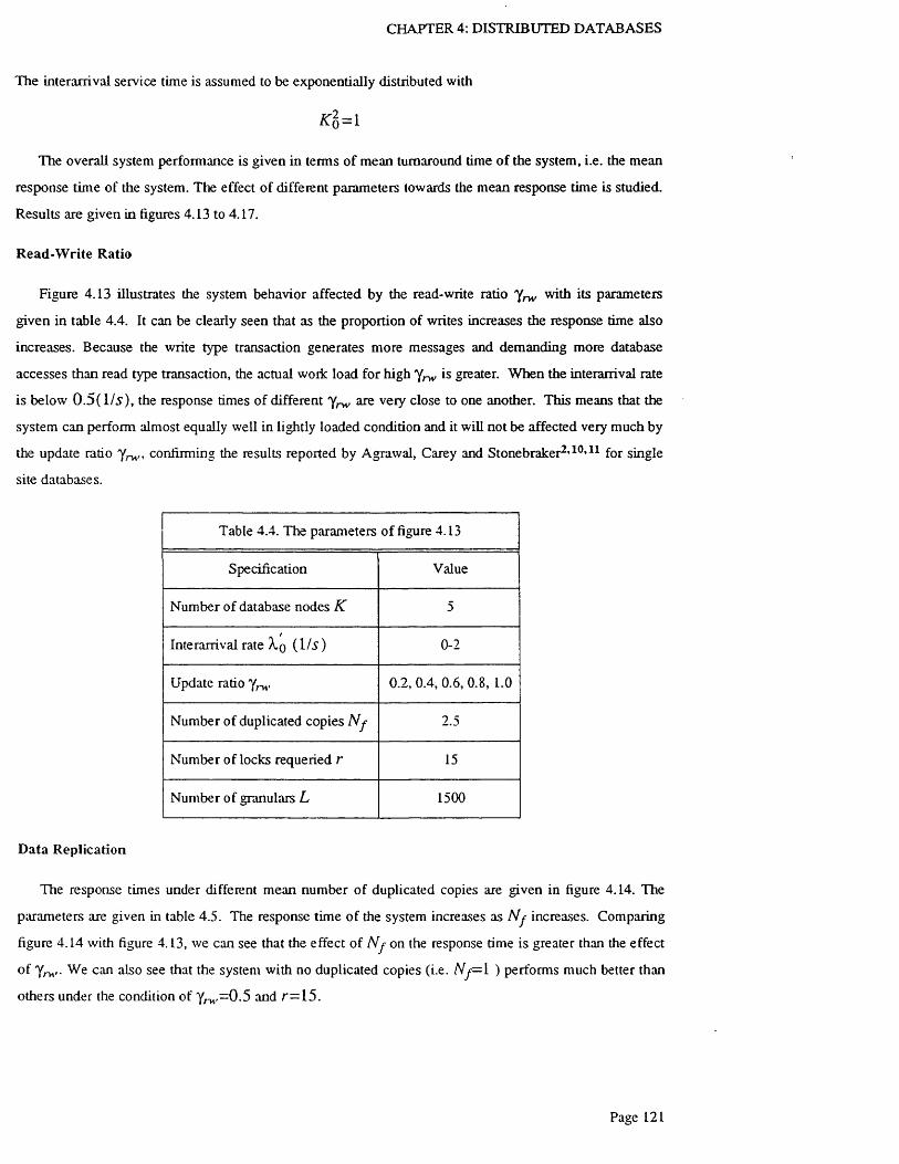
CHAPTER 4: DISTRIBUTED DATABASES
The interarrival service time is assumed to be exponentially distributed with
K \| = L
The overall system performance is given in terms of mean turnaround time of the system, i.e. the mean
response time o f the system. The effect of different parameters towards the mean response time is studied.
Results are given in figures 4.13 to 4.17.
R ead-W rite Ratio
Figure 4.13 illustrates the system behavior affected by the read-write ratio Yrw with its parameters
given in table 4.4. It can be clearly seen that as the proportion of writes increases the response time also
increases. Because the write type transaction generates more messages and demanding more database
accesses than read type transaction, the actual work load for high y ^ is greater. W hen the interarrival rate
is below 0 . 5 ( l / j ) , the response times of different Yrw 316 verY close to one another. This means that the
system can perform almost equally well in lightly loaded condition and it will not be affected very much by
the update ratio Yrw» confirming the results reported by Agrawal, Carey and Stonebraker2,10,11 for single
site databases.
Table 4.4. The parameters o f figure 4.13
Specification Value
Number of database nodes K 5
Interarrival rate (1/5") 0-2
Update ratio Yrw- 0.2, 0.4, 0.6, 0.8, 1.0
Number of duplicated copies N f 2.5
Number of locks requeried r 15
Number of granulars L 1500
D ata R eplication
The response times under different mean number of duplicated copies are given in figure 4.14. The
parameters are given in table 4.5. The response time of the system increases as N f increases. Comparing
figure 4.14 with figure 4.13, we can see that the effect of N j on the response time is greater than the effect
o f Yrw- We can also see that the system with no duplicated copies (i.e. /Vy=l ) performs much better than
others under the condition of Y/-h-= 0 .5 and r= 1 5 .

CHAPTER 4: DISTRIBUTED DATABASES
5
4Response
Time
(in seconds)
2
1
6
5
4Response
Time
(in seconds)
2
1
F igure 4.14. Response Time with Different Replicated Copies N f
Y w = I . o / 0 . 8 / 0 6 ^ 0.4.
.5 1■0Interanival Rate Xq
F igure 4.13. Response Times with Different Read-Write Ratio Yrw
1.50 .5 1Interarrival Rate
Page 122

CHAPTER 4: DISTRIBUTED DATABASES
Response
Time
(in seconds)
Response
Time
(in seconds)
6
5
4
3
2
1
■0 .5 IInterarrival Rate Ao
F igure 4.15. Response Times with Different Granularity r /L
60.25
5
4
3
3 41Mean Number of Replicated Copies N f
F igure 4.16. Response Times vs Nj- with Different Read-Write Ratio
Page 123

CHAPTER 4: DISTRIBUTED DATABASES
0 .0 4 -
0.03
M ean
Conflict
Rate p c0 .0 2 -
0.01 -
2010 155 25Mean Number of Locks V
F igure 4.17. Mean Conflict Rates with Different Replicated Copies A/y
Table 4.5. The parameters of figure 4.14
Specification Value
Number of database nodes k 5
Interarrival rate Xq (1 Is) 0-2.5
Update ratio 7rw- 0.5
Number o f duplicated copies N f I, 2, 3 ,4
Number of locks requeried r 15
Number of granulars L 1500
Lock Granularity
Figure 4.15 shows the effect o f database granularity with the parameters are given in table 4.6. The
mean number of locks for each transaction vs. the total number of granulars is set at 5/500, 15/1500,
25 /2 500 , 3 5 /3 5 0 0 respectively, which simulates transactions with the same data-size but different lock
granularity. The results suggest that coarse granularity performs slightly better than fine granularity under
the condition of 7 ^ = 0 . 5 and N y= 2.5. The results suggest that the effect of the database granularity is
Page 124

CHAPTER 4: DISTRIBUTED DATABASES
relatively small, because of the small locking overhead.
Table 4.6. The parameters of figure 4.15
Specification Value
Number o f database nodes k 5
Interarrival rate (1 /5 ) 0-1.4
Update ratio 7nv 0.5
Number of duplicated copies N f 2.5
Number of locks requeried r 5 ,1 5 , 25, 35
Number of granulars L 500,1500, 2500, 3500
R ead-W rite R atio vs. D ata Replication
Figure 4.16 shows the change of response time with A/y under different y ^ , . It is not surprising that
when all the transactions are of read only type, i.e. 7 ^ = 0 , the response time decrease as the number of
duplicated copies increases. The response time then increases slowly as the number of duplicated copies
increases when the update type transaction only occupies a small portion; yrw—0.'15. When the read-write
ratio Trw grows bigger the response time increases dramatically with N f . This quantitative result can be
used as a guidance for DDBMS system design. When the system is highly update oriented, the optimal
mean duplicated copies should be set to one, which means no duplication at all. The parameters are given
in table 4.7.
Table 4.7. The parameters of figure 4.16
Specification Value
Number of database nodes k 5
Interarrival rate Xq (1 /5 ) 1
Update ratio 7rw- 0, 0.25, 0.5, 0.75, I
Number of duplicated copies A/y 1.0 -4.5
Number of locks requeried r 15
Number of granulars L 1500
Page 125
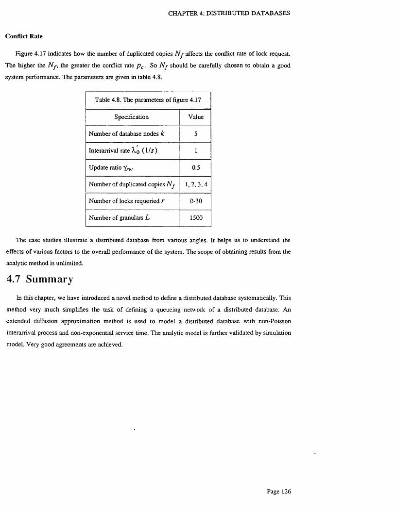
CHAPTER 4: DISTRIBUTED DATABASES
Conflict R ate
Figure 4.17 indicates how the number of duplicated copies N f affects the conflict rate of lock request.
The higher the N f , the greater the conflict rate p c . So N f should be carefully chosen to obtain a good
system performance. The parameters are given in table 4.8.
Table 4.8. The parameters of figure 4.17
Specification Value
Number of database nodes k 5
Interarrival rate A.Q (1 / s ) 1
Update ratio yrA, 0.5
Number of duplicated copies N f 1.2, 3 ,4
Number of locks requeried r 0-30
Number of granulars L 1500
The case studies illustrate a distributed database from various angles. It helps us to understand the
effects o f various factors to the overall performance of the system. The scope of obtaining results from the
analytic method is unlimited.
4.7 Summary
In this chapter, we have introduced a novel method to define a distributed database systematically. This
method very much simplifies the task of defining a queueing network of a distributed database. An
extended diffusion approximation method is used to model a distributed database with non-Poisson
interarrival process and non-exponential service time. The analytic model is further validated by simulation
model. Very good agreements are achieved.

Chapter 5. Major Locking Protocols in DDB
In the previous chapters we have introduced the method to model the performance of basic two phase
locking protocol. However there are quite a few concurrency control protocols based on two phase locking,
among which primary copy 2PL, majority consensus 2PL and centralized 2PL are the most well known
locking protocols used in distributed database. It is the purpose of this chapter to evaluate and compare
these different locking algorithms by using the consistent modeling method introduced in the previous two
chapters and show the integrity of the modeling method by applying it to these popular two phase locking
algorithms.
Section 5.1 evaluates the primary copy 2PL protocol. Section 5.2 estimates the performance o f the
majority consensus 2PL protocol. In section 5.3 the centralized 2PL protocol is modeled. Section 5.4 uses
the analytic results to compare these 2PL protocols.
5.1 Primary Copy 2PL
5.1.1 S y s tem Specif icat ion
The primary copy 2PL is specially designed for distributed databases with replicated data copies76.
One of the physical copies of each logical data item is assigned as the primary copy. Locking can only be
applied to the primary copy. The primary copy 2PL approach simplifies the locking procedure and
prevents dead locks at the cost of extra communication. For example, suppose a logical data item X has
N f copies X i , X 2 , ' ' ' ,Xj , • • • ,Ajv , where X [ is defined as the primary copy. A read transaction
Read (X ) trying to read a copy At other than the primary copy A' has to access the primary copy A' first
to own a read lock at the first phase of two phase commit protocol. It then accesses copy A; and releases
locks on the primary copy A i at second phase of two phase commit. The Read (X ) procedure is shown in
figure 5.1
The Write { X) transaction of the primary 2PL is similar to that of basic 2PL. The only difference is
that locking is perfomied on the primary copy rather than on all the copies. At the first phase of 2PL a
Prepare { X ) is performed on all the copies while only the Prepare ( X ) on the primary copy implies
lock request for data item X. At the second phase o f the 2PL a dm —write (X ), which means a
Write (X ) applied on a physical database by a DM, is propagated to all the copies A,(/’ = L, ...,/Vy), while
only at the primary copy A [ a d m — write ( X ) implicidy releases locks as shown in figure 5.2. The
primary copy 2PL protocol is formally represented as follows:
Primary Copy 2PL Protocol
Page 127

CHAPTER 5: MAJOR LOCKING PROTOCOLS
source lock request locked point lock release sinkStage: 1 2 3 4 5
lock release
tm.
dm-read
R D Y or ABTPRE ACKCMT or ABT
Phase 1 Phase 2
Figure 5.1. Concurrency Control Structure of Read (X ) of Primary Copy 2PL
Phase 1:
1.1 The coordinator T M k sends Prepare ( X ) and lock request (PRE) message to the participants
{ D M i t X e D M i ) .
1.2 Each D M i receives the message. If the primary copy A'i is stored at D M t , it checks for the
requested locks. If all locks are granted and it is willing to commit, then it writes the transaction’s
record in the log and sends a ready (RDY) answer message to T M k . Otherwise it sends abort
(ABT) message to T M k . If the primary copy is not stored at D M t , it simply sends a RDY to
T M k .
Phase 2:
2.1 Upon receiving the answer message RDY or ABT from {D M , , X G D M t }, T M k sends commit
(CMT) message to all {D M , , X s D M j } if all of them have voted RDY, otherwise it writes an
abort record and sends ABT to all {D M t , X & D M i I-
2.2 After receiving the command message from T M k , each D M j writes either an abort or commit
record in log; then executes the transaction and releases the locks at { D M ^ X g D M i }; and sends
the acknowledge (ACK) message to T M k .
Page 128

CHAPTER 5: MAJOR LOCKING PROTOCOLS
source lock request locked point lock release sinkStage: 1 2 3 4 5
lock release
lock request dm-write
dm-write
i-write
RDY or ABTPRE CMT or ABT ACK
Phase 1 Phase 2
F igure 5.2. Concurrency Control Structure of Write (X ) of Primary Copy 2PL
2.3 TMk waits for ACK messages from all {D M t , X e D M X}; then writes a completion record in log.
5.1 .2 M o d e l Definit ion
The modeling method for the primary copy 2PL is similar to that of basic 2PL introduced in chapters 3
and 4. W e shall use the same method to develop models for the primary copy 2PL.
Access Rules
We shall first formally define the read and write rules of the primary copy 2PL.
Definition 5.1: The rules of R ead (X ) issued from TMk are as follows:
• If X y e D M k , l ock (xy ) and d m - r e a d {x y) at D M k\
• If x [ e D M k and X e D M k , lock (x y) at D M ^ x y e D M t ) and d m - r e a d (X) at D M k ;
• If X y e D M k and X s D M k , lock(x y) and d m - r e a d ( x y ) at D M t ( x y e D M j ).
Definition 5.2: The rules of Write (X) issued from TMk are as follows:
• If x y G DMj , lock(x y) and write(xy) at D M j ;
• If x ye DM j and X e D M j , lock(xy) at DMi(x ye DMi) and d m —write {X) at D M j .
Page 129
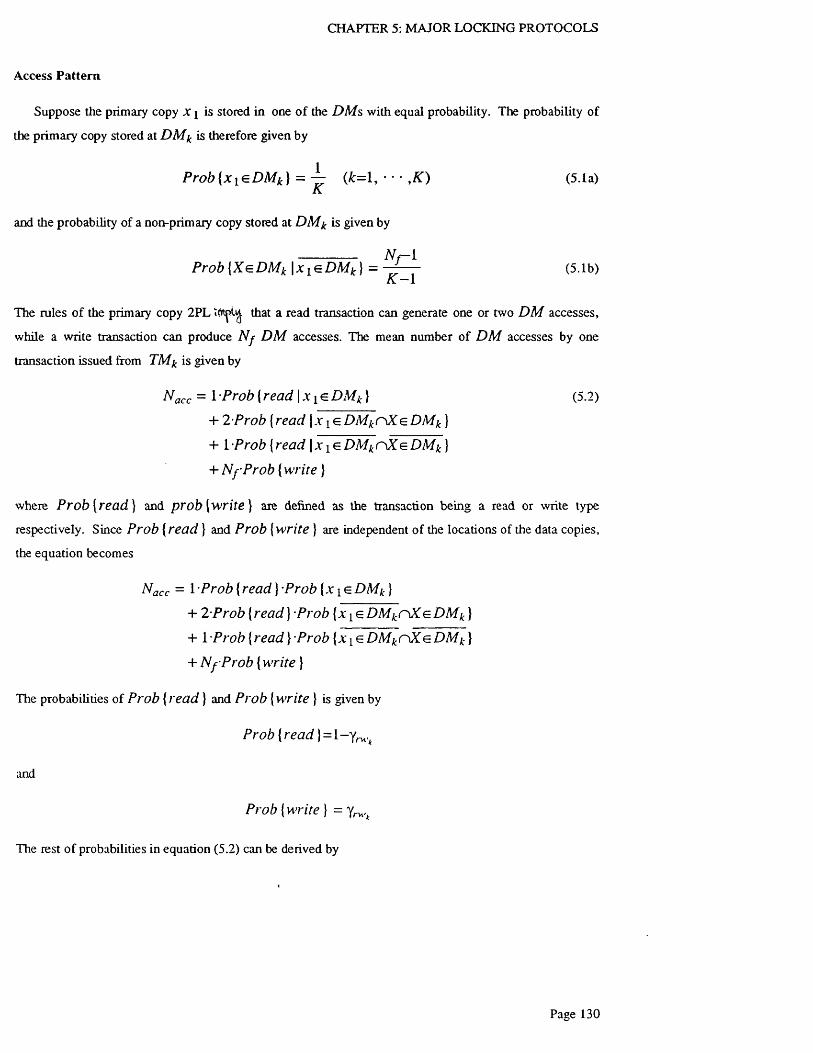
CHAPTER 5: MAJOR LOCKING PROTOCOLS
Access Pattern
Suppose the primary copy X y is stored in one o f the DMs with equal probability. The probability of
the prim ary copy stored at D M k is therefore given by
P r o b { X l s D M k ) = L ( k = \ , ■■ ■ ,K ) (5.1a)K
and the probability of a non-primary copy stored at D M k is given by
N r 1Prob [ X e D M k \ x y e D M k ] = --------- (5.1b)
K —1
The rules o f the primary copy 2PL that a read transaction can generate one or two D M accesses,
while a write transaction can produce N f D M accesses. The mean number o f D M accesses by one
transaction issued from TMk is given by
N acc = 1 Prob {read \ x y e D M k } (5.2)
+ 2 *Prob {read jx y e DM kn X e D M k }
+ 1 'Prob {read \ x y e D M kr S X e D M k }
+ N f P r o b {write }
where Prob [ read] and prob [wri te] are defined as the transaction being a read or write type
respectively. Since Prob [ r e a d } and Prob [write } are independent of the locations of the data copies,
the equation becomes
Nacc - 1 Prob {r e a d } •Prob {* i e D M k }
+ 2 Prob {r e a d } Prob {x y e D M kn X e D M k }
+ l P r o b [ re a d ) -P ro b [ x y e D M kr X e D M k }
+ N f P r o b {write }
The probabilities o f Prob {r e a d } and Prob {write } is given by
Prob [read } = I—yWjt
and
Prob {write } = yw
The rest o f probabilities in equation (5.2) can be derived by
Page 130
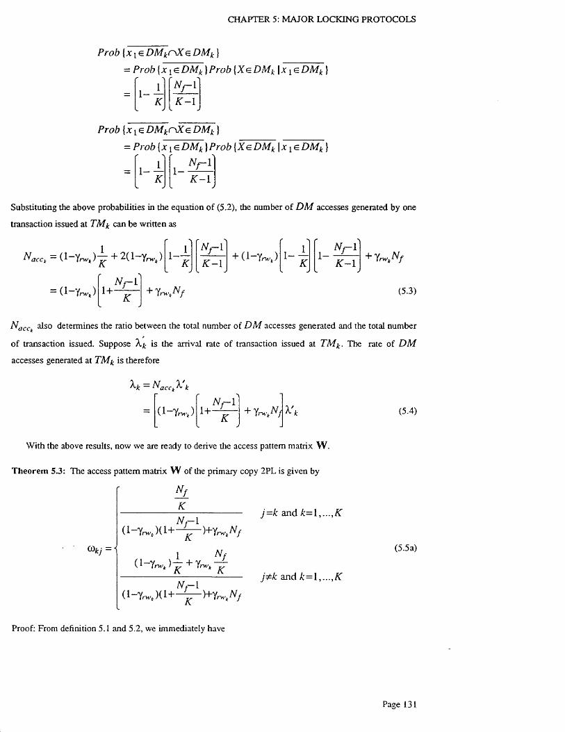
CHAPTER 5: MAJOR LOCKING PROTOCOLS
Prob [ x i e D M kr ^ X e D M k }
= Prob { x l <=DMk }Prob { X e D M k \ x i e D M k }
K
N r l
K - 1
Prob {x L e D M k(XXe D M k }
= Prob {* i e D M k }Prob [ X e D M k \ x \ e D M k
1 -K
1 -N f - 1
K - 1
Substituting the above probabilities in the equation o f (5.2), the number of D M accesses generated by one
transaction issued at TMk can be written as
Nacct = (1 -Xrwt) ~ + 2(1 ~ Y ) 1 - J -K
Nr 1
K - 11 - ^
K1 -
N f —1
K - 1
= ( 1 - Y r w t ) 1 +N r 1
K+ l n , ; N f
+ y.rwt N f
(5.3)
NacCk also determines the ratio between the total number of D M accesses generated and the total number
o f transaction issued. Suppose Xk is the arrival rate of transaction issued at TMk. The rate of D M
accesses generated at TMk is therefore
^ k ~ N acc \ ' k
(1-YTM,) 1+Nr \
KX'l-
With the above results, now we are ready to derive the access pattern matrix W.
(5.4)
T heorem 5.3: The access pattern matrix W of the primary copy 2PL is given by
Nf_
K
N t- 1( 1 “ Y / - w , ) ( 1 + ) + Y m v *Nf
1 Nf ( Y + Yrw't ^
Nf—i(l~Y -u 't. ) ( ! + — ^ ) + Y
j - k and k = l , . . . , K
j ^ k and K
(5.5a)
Proof: From definition 5.1 and 5.2, we immediately have
Page 131

CHAPTER 5: MAJOR LOCKING PROTOCOLS
tokk = Prob {Access kk \ x i e D M k }Prob {jc l e D M k ] (5.5b)
+ Prob [Accesskk Ix 1e D M kn X e D M k }Prob { a i e D M kn X e D M k }
+ Prob {Accesskk | x i e D M kn X e D M k } Prob {x i e D M kc X e D M k }
Under the condition of {A i E D M k } both dm — r e a d (X ) and d m — wri te (X ) need to access node
D M k. The probability of access is
P rob{A ccesskk \ x i e D M k }Prob { x i e D M k ) =1 Prob {r e a d } + 1 Prob {w r i t e }
N,acck
If there is a nonprimary copy in D M k, i.e. {x \ E D M kC\XE D M k }, the dm —read (X ) accesses D M k
to read and the dm —write (X ) accesses D M k to write. The probability of access is given by
1 •Prob {r e a d } + 1 •Prob {write }Prob {Access & | x i e D M kr X e D M k } =
Nacck
If no copy is stored at D M k, there is no need to access it. Therefore
Prob {Accesskk | a ^ e D M kr X e D M k } = 0
Substituting the above probabilities into the equation of (5.5b), we can immediately obtain
1 Prob {r e a d } + 1 •Prob {w r i t e } 1<&kk = N.acck K
+
+
1 Prob {r e a d } + 1 Prob {write }N.acck
O'Prob {r e a d } + O Prob {write
1
NQCCk
1
Nacck
+K
Nf
~K
N,
1 - — K
Nf—i
K - 1
Nf_
KN f - 1
( 1 Yrvi'i )( H ^7~)+YrM't N fK
1 -K
Nr l
K - 1
Nr [
K - 1
Similarly
cokj - Prob {Accesskj \x \ e D M j } Prob {x i e D M j }( J * k )
+ Prob {A c c e s s kj | ,v i e D M j n X e D M j } •Prob {x y e D M j n X e D M j }
+ Prob {A c c e s s kj | a i e D M j C \ X e D M j } •Prob {x \ e D M j n X e D M j }
(5.5c)
Page 132

CHAPTER 5: MAJOR LOCKING PROTOCOLS
Under the condition of [ x i g D M j ) read and write transaction will both access the primary copy at
D M j , that is
Prob {Access^ \ x i e D M j }1 Prob {r e a d }+1 •Prob {write }
1
N ,
The case of {*i e D M j C S X ^ D M j } deserves some comments. According to the read rule of the primary
copy 2PL, a read transaction will access the primary copy and the local copy. In this case, Read (X ) will
not access D M j , since the primary copy is not stored at D M j and D M j is not a local node ( J & k ).
Therefore we have
Prob = {Access kj \ x i e D M y n X e D M j } 0 Prob {r e a d } + 1 •Prob {write }
Yrw**
a ^ 7
under the condition of { x \ e D M j n X s D M j } there is no need to access D M j . That is
Prob {Access kj I x i e D M j n X e D M j } = 0
Substituting the above probabilities to equation (5.5c), we have
1i - L
K
N f —l
K - 1+ 0
the primary copy 2PL can be constructed in the same way as that of the basic 2PL system. The overall
structure of the queueing network model is shown in figure 4.2.
With the newly derived access pattern matrix W , the arrival rate matrix and the Markov chain matrix
of the primary copy 2PL queueing network model can be obtained by using the communication flow
method introduced in section 4.2.2. The arrival rates are given by
A o - %2 ' ' '
N a c c M A acc i ^ K (5.6a)
A i = V A r (5.6b)
A,iCOu+A,2CD21+---+^/s:a)A: 1 ^ l ( l 2 +^ 2 ()>22+ '--+^ K ( K 2 ' ' '^ ltoiK +A ,2C 02/C +..-+A .£G )o:
Page 133

CHAPTER 5: MAJOR LOCKING PROTOCOLS
A2 = V A 2 (5 .6 c )
A,i(Oii+A.2 (Oi2 +...+X ^C O i^ X 1 C0 2 i+A.2 C0 2 2 +"-+^A:a>2A' ' * * ^ l to/ n + ^ 2 w K 2 + *"+ ^ £ tt>i a :
A 3 = Vr A 3 (5.6d)
XiCOu+A<2(02i+...+A.^CO/^i A.1C0i2+^'2C022+ -*-+^/s:C0A:2 * ’ ' t t ) l A T + ^ - 2 ■ -+ ^K ^K K
A 4 = Vr A4 (5.6e)
XiC0h+A,2C0i2+...+X,^C0i^ ^1 ©2i+A,2&22~^~"-'^‘K®2K. ’ ' ' ^1
and the communication flow matrix is given by
A c = £ A ,
J = 12 A,j C0 j_j[
( 5 - 6 0
= 2
A.2 t0 2 i"b^'i tO}2
I l ( 0 i 2 + X 2 ®2 i 2 X,2 C0 2 2
^ K ^ K l + ^ l t o l K
2+^*2 &2K
2 \ K (£tKK
and the Markov chain matrices are given by
P =Pj 0 “
o Po (5.7)
Locking
The primary copy 2PL locks only the primary copy of the logical data item. It generates less locking
activities in a distributed database system than the basic 2PL algorithm.
Suppose the mean number of locks required by a transaction at T M ^ is denoted by r*. A transaction
generates an average of Nacc D M accesses, where Nacc is defined as the mean number of D M accesses
by on transaction.
Kn = v ni y acc / , 1Yqccl
k = 1
Only one of them requires locks on the primary copy. If we observe the system from the view point of
each DMfc(k = {,. . .K), one out of Nacc accesses is to request locks, which means that only one out of
Nacc arrivals to a D M node needs locking service. Therefore the actual arrival rate of the lock request
centre is equal to
h =kK+1 (5.8)
Page 134

CHAPTER 5: MAJOR LOCKING PROTOCOLS
Substituting the above equation into equation (4.55), the mean number of locks held at the lock request
centre can be modified as
N i ^ o c k ) _r*_ 1
(7 k ^acc 1— 1(5.9)
The mean number of transaction execution (i.e. d m —r e a d (X ) and d m —w r i te ( X ) ) generated by
one transaction is given by
where
N ex = 1 'P ro b {r e a d } + N f P r o b {w r i t e }
1 — Y nv N fff-w
K Yrw* Y nv= Z
(5.10)
A=1 K(5.11)
It should be noted that only N ex out of N acc D M accesses involve with transaction executions; while the
rest only involve with releasing locks, which means that only N exINacc percent of the transactions enter
the transaction execution centre. The actual arrival rate of the transaction execution centre is therefore
N„Xi-kK+2 vr k/c+2
4 V nrr-
At the execution stage, only one out of N acc transactions holds locks. The actual number of locks held at
the execution stage is
N L [ex) = — nkr ,h i k K+2
acc(5.12)
Similarly at the communication stage, only one out of N acc transactions holds locks. The modified number
of locks held at the communication stage is therefore
w 4 'com 2) _ rk
NL<tcom 3 ) _
Nacc
£ ^ - 1Sir*:£ < 4 3 ) - '
1=1 ^ tk
(5.13a)
(5.13b)
Now we have got all the necessary equations to solve the probability of the locking conflict q
NL]!ock) + t i L [ coml) + N L {£ oml) + N L [ ex)i - q k =
L ,
Substituting equation (5.9), (5.12), (5.13a) and (5.13b) into the above equation, we immediately have
Page 135

CHAPTER 5: MAJOR LOCKING PROTOCOLS
4 -1
Z +r/c
1 - ^ - =<=L
r * « g > _ 4 ? - l+ ' 1*.
A r=I a:
Diffusion Approximation Queueing Network Solution
Applying the diffusion approximation method introduced in section 4.4 to the primary copy 2PL medel,
we can obtain the following results. The relative throughput of the queueing network can be derived from
its M arkov chain matrix given by equations (5.7). Let et be the relative throughput at service centre i,
where
*i = P o i + ' Z e j P j i 7=1
m = K ( K + 2 )
(5.14)
is the total number of service centres in the open distributed database queueing network. The arrival rate of
service centre i is proportional to the relative throughput.
'ki = X0 ei (z = l , ■ ■ ■ ,m)
The utilization of the service centre i is
Xoei
(5.15)
PiPi
, i f Xoe,•<}!,• ( z = l , . . . ,m ) (5.16)
Under the condition of heavy traffic, the total number of arrivals to station i in the interval [0 ,f ] will
be normally distributed with mean A.,-f and variance
' £ [ ( . C j - l ) p j i + l ] k j P j i t (5.17)7 = 0
where Cj is the squared coefficient of the variation of the interarrival time at service centre j.
By constructing the diffusion approximation to the length of individual queue, where f i ( X i , t ) is the
density function approximating the length of the M h queue, the stationary solution of the diffusion
approximation equation is given by
P i(e — 1 >6’ 'X' , * ;> 1
p t(l-<?Y,A‘ ), 0<x,-<l(5.18)
where
Page 136

CHAPTER 5: MAJOR LOCKING PROTOCOLS
Y, = -2 p ,/ tt , (5.19)
The parameters of the above equations are given as,
Pi = Xi - [l; (5.20)
ma , = p i i i i K f + X [ ( .C j - V p j i+ U X jP j i (5.21)
j=o
The squared coefficient o f variation of the interarrival time C /, 0 = 1 , ' * * , t n ) can be obtained
numerically by solving a system of linear equations
( i - p , ) « , p( C , - l ) - - ------— j X ( C j - D X j p j i = — ------------ r- (1 = 1 ....... m ) (5.22)
^ • + ^ iP / / ( l - P i ) ;=0J« l - ( l - p , ) p , ;
where ^ is the squared coefficient of variation of the service time distribution at service centre i.
The lock request service centre jfc+i ui figure 4.2 is a IS service centre which can be represented by a
single server service centre with service capacity' equal to ^ /N jK+i\ l jK+i ( j = 1 , Fr om equation
(4.112) the throughput of lock request service centre j'k +i can be given by
Pjk+\ = ^ 7ic+i ^Y / *+1 (5.23)
where N j K+ is given by equation (4.113) and rewritten as
o l .
" a . , = { (Cj*-, + + 1) (5.24)1*7*+1
C j is the squared coefficient o f the variation of the interarrival time at service centre //c+l> which
equals to the sum of the independent variance of the interdeparture time of all the other service centres to
centre j K+[.
1 mC jK+x ~ Z £ + 1 X i P i j K+l (5.25)
7/c+i i=0
Substituting equation (5.8), (5.24) and (5.25) into equation (5.23), we can obtain p j . The
approximate average queue length can be therefore given by
= Pi i - *2 P,
Applying Little’s law, the average turn-around time of the system is
Page 137

CHAPTER 5: MAJOR LOCKING PROTOCOLS
™ n;^ = I r - (5.26)
1 = 1 ^ 0
5 .1 .3 P erform ance R esults
The parameters of the evaluation of the primary copy 2PL system are the same as basic 2PL. They are
given by table 4.3 to 4.8.
The overall system performance is given in terms of mean turnaround time of the system. The effect of
various parameters towards the mean response time is studied and illustrated in figure 5.3 to 5.8.
R ead-W rite Ratio
Figure 5.3 illustrates the system behavior affected by the read-write ratio Yrw - Its parameters are given
in table 4.4. It shows clearly that the system performs better under smaller y,^,, i.e. more read type and less
write type transactions. When the range of interarrival rate is below 0.5 ( l / s ) , the response times of
different y ^ , are very close to one another, which means the system can perform almost equally well in
lighdy loaded condition without being affected by the update ratio yw .
D ata Replication
The response times under different mean number of duplicated copies are given in figure 5.4. The
parameters are given in table 4.5. Its pattern is very similar to that o f basic 2PL in figure 4.14. But there is
an intersting phenomenon at the range 0<X < 0 .25 . The choice of no replication is the least favorable
among others. X —>0.25 is a turning point. The reason behind this is that when work load is small there is
no queueing at the transaction execution and data communication centres. High replication can increase the
chance of local access but not necessarily the processing time. Therefore high data replication can reduce
the response time. As the work load builds up, queues will form more rapidly for higher replicated system.
Thus the performance tends to favor lower replication.
Lock G ranu larity
Figure 5.5 shows the effect o f database granularity with parameters given in table 4.6. The mean
number of locks for each transaction vs. the total number of granulars is set at 5/500 , 15/1500,
2 5 /2 5 0 0 , 3 5 /3 5 0 0 respectively. The results show that the difference between coarse and fine granularity
is even smaller than that of basic 2PL in figure 4.15, because locking is only performed on primary copies.
The effect o f granularity on performance is related only to the lock processing times at the sites of primary
copies.
R ead-W rite Ratio vs. Data Replication
Figure 5.6 shows the change of response time with N f under different y ^ ,. The decrease in response
time towards high replication is more obvious for the primary copy 2PL than that for the basic 2PL. When
Page 138

CHAPTER 5: MAJOR LOCKING PROTOCOLS
5
4Response
Time
(in seconds)
2
1
6
5
4Response
Time
(in seconds)
2
L
Figure 5.4. Response Time with Different Replicated Copies N f
0 .6, 0.4
■0 1.5LInterarrival Rate Xq
F igure 5.3. Response Times with Different Read-Write Ratio
0 15 1.5Interarrival Rate
Page 139

CHAPTER 5: MAJOR LOCKING PROTOCOLS
Response
Time
(in seconds)
Response
Time
(in seconds)
5 -
4 -
3 -
2 —
1■0 .5Interanival Rate
F igure 5-5. Response Times with Different Granularity r ! L
0.5/'
4 -
2 _
421
Mean Number of Replicated Copies N f
Figure 5.6. Response Times vs N f with Different Read-Write Ratio
Page 140
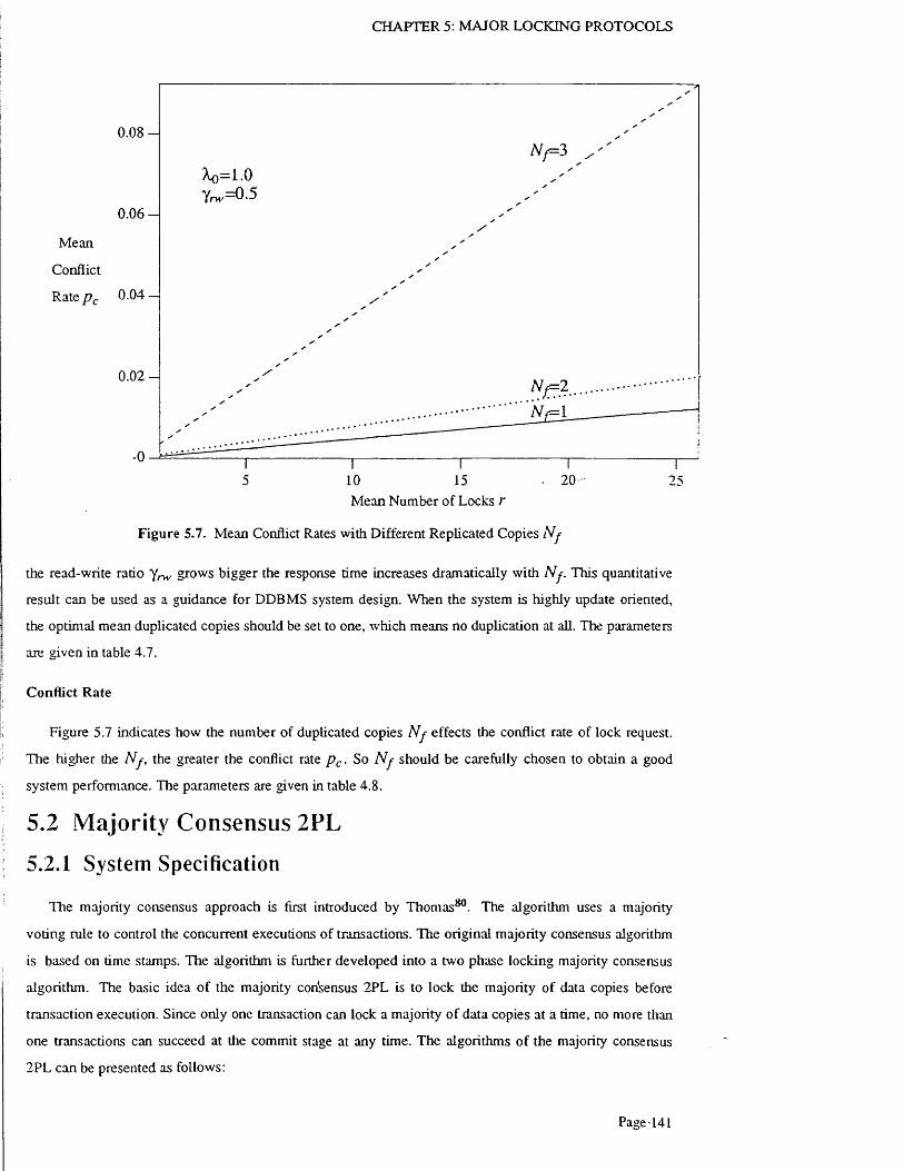
CHAPTER 5: MAJOR LOCKING PROTOCOLS
0 .0 8 -
0 .0 6 -
Mean
Conflict
Rate p c 0.04 —
0 .0 2 -
20105 15Mean Number of Locks r
F igure 5-7. Mean Conflict Rates with Different Replicated Copies N f
the read-write ratio grows bigger the response time increases dramatically with N f . This quantitative
result can be used as a guidance for DDBMS system design. When the system is highly update oriented,
the optimal mean duplicated copies should be set to one, which means no duplication at all. The parameters
are given in table 4.7.
Conflict Rate
Figure 5.7 indicates how the number of duplicated copies N f effects the conflict rate of lock request.
The higher the N f , the greater the conflict rate p c . So N f should be carefully chosen to obtain a good
system performance. The parameters are given in table 4.8.
5.2 Majority Consensus 2PL
5.2.1 System Specification
The majority consensus approach is first introduced by Thomas80. The algorithm uses a majority
voting rule to control the concurrent executions of transactions. The original majority consensus algorithm
is based on time stamps. The algorithm is further developed into a two phase locking majority consensus
algorithm. The basic idea o f the majority consensus 2PL is to lock the majority of data copies before
transaction execution. Since only one transaction can lock a majority of data copies at a time, no more than
one transactions can succeed at the commit stage at any time. The algorithms o f the majority consensus
2 PL can be presented as follows:
Page 141
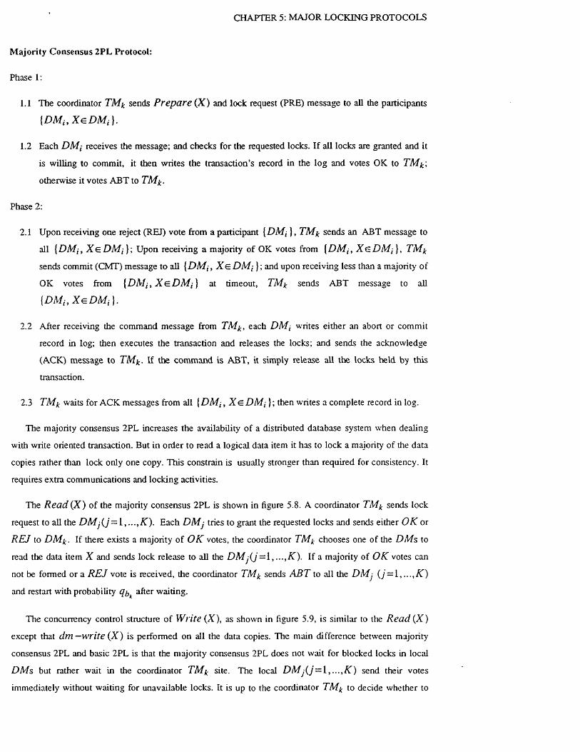
CHAPTER 5: MAJOR LOCKING PROTOCOLS
M ajority Consensus 2PL Protocol:
Phase 1:
1.1 The coordinator T M ^ sends P r e p a r e (X ) and lock request (PRE) message to all the participants
{D M h X e D M i }.
1.2 Each D M i receives the message; and checks for the requested locks. If all locks are granted and it
is willing to commit, it then writes the transaction’s record in the log and votes OK to TM^',
otherwise it votes ABT to TM^.
Phase 2:
2.1 Upon receiving one reject (REJ) vote from a participant {D M ,•}, TM* sends an ABT message to
all {DMi, X e D M i }; Upon receiving a majority of OK votes from {DM± , X s D M ;}, TM^
sends commit (CMT) message to all {DM-t , X e D M ; }; and upon receiving less than a majority of
OK votes from {D M t , X e D M ; } at timeout, 7"M* sends ABT message to all
{ D M ;,X e D M ;} .
2 . 2 After receiving the command message from T M each DM; writes either an abort or commit
record in log; then executes the transaction and releases the locks; and sends the acknowledge
(ACK) message to TM^. If the com m and is ABT, it simply release all the locks held by this
transaction.
2.3 T M k waits for ACK messages from all {D M ;, X e D M ; }; then writes a complete record in log.
The majority consensus 2PL increases the availability of a distributed database system when dealing
with write oriented transaction. But in order to read a logical data item it has to lock a majority of the data
copies rather than lock only one copy. This constrain is usually stronger than required for consistency. It
requires extra communications and locking activities.
The Read (X ) of the majority consensus 2 PL is shown in figure 5.8. A coordinator T M ^ sends lock
request to all the DMy(y = 1, .. . ,X ) . Each D M j tries to grant the requested locks and sends either O K or
REJ to DMfr. If there exists a majority o f O K votes, the coordinator T M ^ chooses one of the DM s to
read the data item X and sends lock release to all the D M j ( J = \ . , . . . ,K ) . If a majority of O K votes can
not be formed or a REJ vote is received, the coordinator T M ^ sends A B T to all the D M j ( j = [, . . . ,K )
and restart with probability <7^ after waiting.
The concurrency control structure of Write (X ), as shown in figure 5.9, is similar to the Read (X )
except that d m — write (X ) is performed on all the data copies. The main difference between majority
consensus 2PL and basic 2PL is that the majority consensus 2PL does not wait for blocked locks in local
D M s but rather wait in the coordinator T M ^ site. The local D M j ( j = l , . . . , K ) send their votes
immediately without waiting for unavailable locks. It is up to the coordinator T M % to decide whether to

CHAPTER 5: MAJOR LOCKING PROTOCOLS
source lock request locked point lock release sinkStage: 1 2 3 4 5
waiting
blocked queuedm dm
lock release dm/readlockrequest
dm-readtm. trrt
•read
dm
PRE RDY or ABT CMT or ABT ACK
Phase 1 Phase 2
F igure 5.8. Structure of. Read {X) of Majority Consensus 2PL
commit or abort according to the result of the voting. If a majority of O K votes can not be obtained, the
coordinator T M ^ releases all the locks and restarts the transaction after waiting.
5 .2 .2 M odel Defin ition
Access Rules
We shall give a formal definition of the read and write rules of the majority consensus 2PL as follows:
Definition 5.4: The rule of Read (X ) issued at T M £ is as follows:
• if X e D M j , lock(X) and dm - r e a d (X ) at D M j .
The rule of Write (X) is as follows
• if X e D M j , lock ( X ) and d m - w r i t e { X ) at D M j .
Access P attern Suppose the data copies are uniformly stored in distributed database. That is
NfProb { X G D M k } =
Page 143

CHAPTER 5: MAJOR LOCKING PROTOCOLS
source Stage: 1
lock request2
locked point 3
lock release
4
sink
5
waiting
blocked queuedm dm
lock release dm-write
lockrequest
dm-writetrri
dm-Vrite
dm dm ,
PRE RDY or ABT ACKCMT or ABT
Phase 1 Phase 2
Figure 5.9. Structure of Write (X ) o f Majority Consensus 2PL
The probability of a transaction at T M ^ being read or write oriented are respectively
Prob {read} = 1 - y Wt
and
Prob {write } =
Since read and write transactions both require Nf D M accesses, the total number of DMs accessed
by one transaction is simply given by
N acc = N f P r o b {r e a d } + N f P rob { write
= N..f (5-27)
Be applying the same method to the majority consensus 2PL, the access pattern matrix can also be
easily obtained by the following theorem.
T heorem 5.5: The access pattern matrix W of majority consensus 2PL is given by
Page 144

CHAPTER 5: MAJOR LOCKING PROTOCOLS
(5.28)
Proof: (0 kj is defined by
cojtj = Prob [Access^ \ X e D M j }Prob [ X e D M j
+ P rob {A c c e s s ^ IX e D M j } Prob {X e D M j }
1 Prob [ X e D M j )N,
1 N f
Nacc K
J _
K
Hence [ ].
A rrival Rate M atrix
As we can see from figure 5.8 and 5.9 the blocked transactions will enter the blocked restart after a
waiting delay. The probability of a transaction entering the blocked queue at T M k is denoted by q\yk. The
virtual arrival rate of D M k is therefore equal to the sum of the original arrival rate N accX 'k and the restart
rate q b j^ a c c ^ k > that is
'W = N acc\ ' k + ( 1 - q b t )N aCc X 'k
= { 2 - q bi)Nf X'k
The arrival rate array at the source point is therefore
A q - •K
(5.29)
(5.30a)
The arrival rate to the blocked queue centre is given by
b x 0
A * — A q
0
0 0
• 0
• 0
•• l-<7 bk
(5.30b)
The arrival rates at the other queueing centres are
= V r A l (5.30c)
A,iG3ii+A2<i)21+"-+A,£<X) £ - 1 A.iC0i2+A2CO22+...4-A.^(O^2 ' ' ' A.iCOi^+A2 CL>2 /f+ ...+ A /^C O ^
Page 145

CHAPTER 5: MAJOR LOCKING PROTOCOLS
A 2 = Vr A 2 (5.30d)
^iC01i+ ^ 2C0i2-+-...+X/j:C0iA: A4 CD21+A.20022+ . . .+ ^ (£>2K ' ' ' l + ^ 2 (° K 2 + -"+ ^ K (£iK K
a 3 = v r A 3
Aq CO11 + ^ 2 ( 0 2 ! + . . .+ A .£ (D £ i Aq ( O i2 + ^ 2 a )2 2 + - • 2
A 4 = Vr A<
XiC011+A,2C012-I-...+Xx-C0i^ X1(02i + ^ 2C 0 2 2 + -+ ^ C02A:
and the communication flow matrix is given by
(5.30e)
• A q CO i k + ^ 2 C0 2K + • • -+ ^ K t&KK
(5.30f)
^ 1 &K 1 + ^ 2 2 + • • -+ ^K tofCK
A c = E A f5 = 1 __
2 A q c o ^ i
(5.30g)
= 2
M arkov C hain M atrix
/»2 CC>2 i + A i C0 | 2
A.1 CO1 2+A.2 CO21 2 A.2 CO22
^ i coi/i:+ ^/s:co/ : i A2 co^ 2
Aatcoa: iH-Ai coi/^
2 + ^ - 2 (J 2K
2 \ k (£>k k
For the majority consensus 2PL there is an additional path from the sink point to the blocked queueing
centre and from the blocked queueing centre to the source point with probability P ^ ) p ( ^ )
respectively. Suppose m is the total number of service centres and stage points defined in the Markov chain
matrix. is a (m —K ) x K matrix defined by
n KsP)P t j - 1 0
'qy. i f i e (sink at TMk) and j e (blocked queue at TMk)
i f otherwise (5.31a)
where p \ Sj* can be interpreted as the probability of a transaction going from the sink point at TMk to the
blocked queue at TMk, and P ^ 5 is a K x ( m —K ) matrix defined by
f 1 if i e {blocked queue at TMk) and j e (source at TMk)
^ S )= |o a o therw ise (5'31b>
where p^j5 is the probability o f a transaction moving from the blocked queue at TMk to the source point
at TMk. Combining P ^ ^ and P ^ ^ with the input and output matrices P / and P q , the overall Markov
chain matrix can be obtained byp / 0
p (^ TP J 0
0 P o
p(fo) 0(5.31c)
Page 146
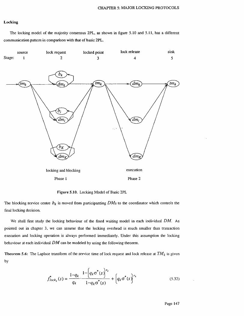
CHAPTER 5: MAJOR LOCKING PROTOCOLS
Locking
The locking model of the majority consensus 2PL, as shown in figure 5.10 and 5.11, has a different
communication pattern in comparison with that of basic 2PL.
source lock request locked point lock release sink
Stage: 1 2 3 4 5
drrii
dm ,d m
locking and blocking execution
Phase 1 Phase 2
F igure 5.10. Locking Model of Basic 2PL
The blocking service centre is moved from participanting D M s to the coordinator which controls the
final locking decision.
We shall first study the locking behaviour of the fixed waiting model in each individual D M . As
pointed out in chapter 3, we can assume that the locking overhead is much smaller than transaction
execution and locking operation is always performed immediately. Under this assumption the locking
behaviour at each individual D M can be modeled by using the following theorem.
T heorem 5.6: The Laplace transform of the service time of lock request and lock release at TMf- is given
by
-
f lo c k k ( s ) =i - q k
<ik
l - q ka ( s )
1 - q ka (s)+ q k<5 ( s ) (5.32)
Page 147

CHAPTER 5: MAJOR LOCKING PROTOCOLS
source lock request locked point lock release sinkStage: 1 2 3 4 5
blocking
drrii d m t
dm, dm ,
locking execution
Phase 1 Phase 2
F igure 5.11. Locking M odel o f Majority Consensus 2PL
and the m ean is given by
1 1
\^-lock M'S(5.33)
ijcwhere q^ is the probability of successfully granting one lock and <5 ( s ) is the Laplace-Stieltjes transform
of the service time distribution o f one locking operation.
Proof: To produce a OK vote each D M must obtain r * locks. The request o f each lock can be modeled by
an infinite-server service centre as introduced in chapter 3. A transaction at D M * will successfully grant a
lock with probability q as illustrated in figure 5.12. It is due to Cox17 that a system with stages has
the following Laplace transformation
r*_I ' *f iockk CO = £ <7o • * • q i - i P i U a * ( s )
/ =0 /=1
where p i —i —q t . Since the locking system has at lease one and at most /*£ lock request stages,
Page 148

CHAPTER 5: MAJOR LOCKING PROTOCOLS
Figure 5.12. Blocking Model
<70= 1 ; Po =0;q rt_ i = 0 ; ; p r^ = 1
Furthermore the success probability q t ( z = l , • * * , r k —1) at the different stages of lock request are
approximately identical under the condition of r k <gJLk (& =1, ' • • , K ) . The success and conflict
probability q± and p i (z = 0 , • • • t r k— 1 ) are
q-i = qP i = 1 - q z '= 0 ,...fr * - l
Let us denote qk—q as the success probability at D M k . Substituting q t and p t into the original equation,
we can further derive
r*_1f lock k ( ^ ) = ' L q lk~l ( i - q k ) ( v * ( s ) y +
i=0r
i - q kl - q k< y '(s )
qk 1— ( s )+
q r io \ s )
qk-o* ( s )
Hence [ ].
The mean o f f ock( s ) is given by
1 d f ock( s )
\^lock d s
l-<7* - n l qko * V ) 1 - q kG* (s )J
- - q ko * \ s ) l - ( q k f ( s ) ) rt
qk ( 1 - q ka ( s ) ) 2s = 0
q k < f Cs)|r* 1 q k < f \ s )s = 0
Since
Page 149
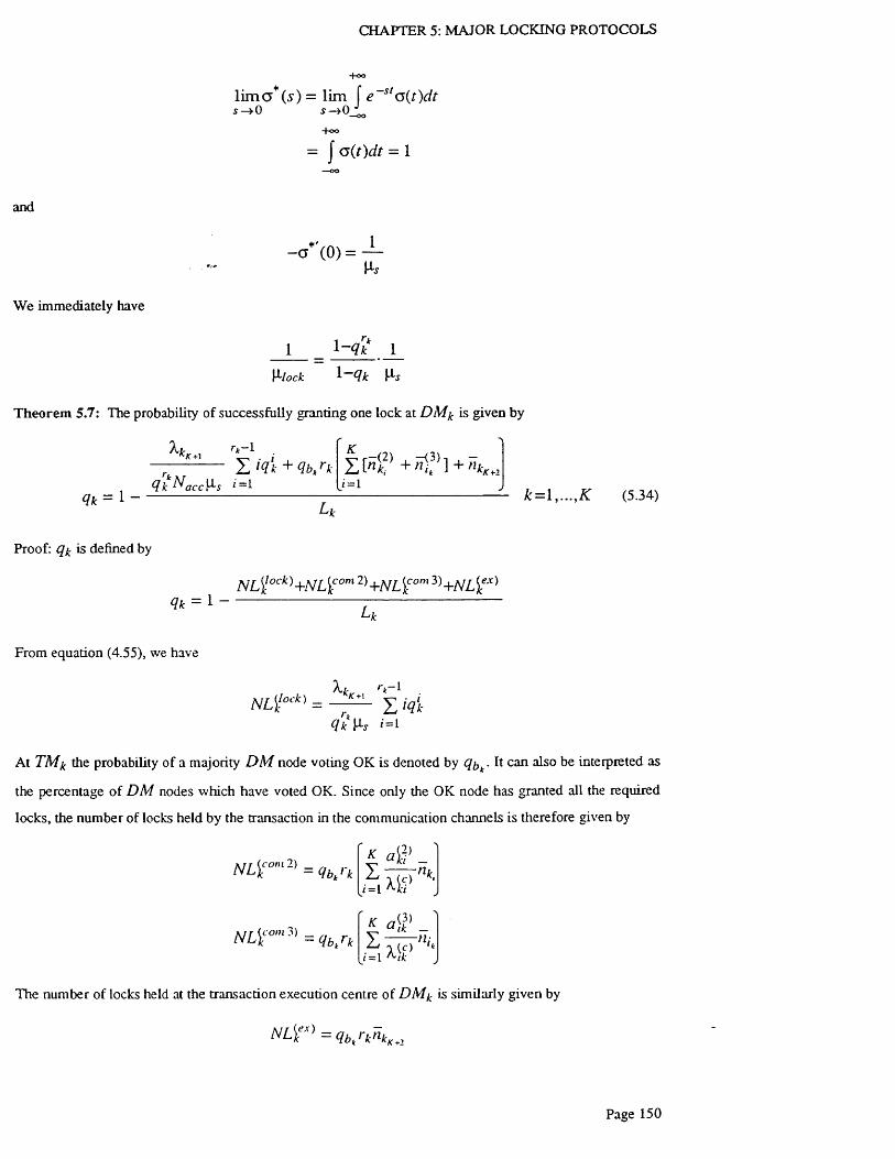
CHAPTER 5: MAJOR LOCKING PROTOCOLS
-foo
S —>0lim a*(5’) = lim f e st<5(t)dt
-h o o
= I a(t)dt = 1
and
- a (0) =M®
W e immediately have
1 1 ~q{ 1\^lock 1 Qk Mm
T heorem 5.7: The probability of successfully granting one lock at D M ^ is given by
Krk~ l
Q k ^ a c c ^ s *■— 1Z ' Q k + Q b j k
Qk= 1 -
Proof: is defined by
Qk = l ~
From equation (4.55), we have
i = l
N L ]! ock)+ N L [ com 2)+ N L [ com 3)+NL<kex)
L k
k = l , . . . tK (5.34)
NL]!lock) __A.k/C+\
rt - 1
Qk i — 1
S iq'k
At T M k probability of a majority D M node voting OK is denoted by . It can also be interpreted as
the percentage of D M nodes which have voted OK. Since only the OK node has granted all the required
locks, the number of locks held by the transaction in the communication channels is therefore given by
K 4 ; ’ _- Q b j k Z
<=i W
K 4 3) _= Q b / k z;=i W n 'k
N L ^ ° '
The number of locks held at the transaction execution centre of D M * is similarly given by
N L ^ = q b J k n kKtl
Page 150

CHAPTER 5: MAJOR LOCKING PROTOCOLS
The total mean number of D M * held is therefore equal to
'hfc rk~ 1NL<t ck) + NL^am2) +NL{c°m}) +NL[ex) = £ iq\ + q btrk
Qk mZ [Hi2’ + f 3) ] + nk
i = 1
and the total number o f granules at D M ^ is equal to L^. Hence
'X.i rk- 1
^ = 1 “
Z lRk + <7*/*£ + x£>
[].
Next we shall derive the locking behaviour at the coordinator site TM. As mentioned previously the
locking decision is made at the coordinator site TM according to the OK or REJ votes received from the
participants D M £ ( £ = ! , * • • , K ). If any REJ votes is received or a majority of OK can not be formed,
the transaction enters the blocked queue at TM. The probability of the blocking and the duration of the
blocking are derived in the following two theorems.
T heorem 5.8: The probability of non-blocking at T M is given by
i f )
96, = 1 - Z n Qk n 1 -q ’k k=l , . . . ,Kj = l DMke O K ( j ) DMke O K ( j )
(5.35)
where O K (J) denotes the set o f j DMs which vote OK.
Proof: In order to obtain a majority of O K votes from DMi(i = \ , . . . , ,K) , there must exist more than
A ^/2 D M nodes which can grant all required locks. The probability of successfully granting one lock at
DMfr is Thus the probability o f successfully granting / f locks at D M ^ is . The probability of
getting j O K votes is
Prob {O K v o t e s = j } = n rkRk n
DMt<=OK(j) DMke O K ( j )\~Rk
And the probability of not getting a majority of O K votes becomes
Nf
NflT ]
Prob {O K votes < — } = Prob {O K votes - j }
Nr, t f ]
= Z n Q^ n l~Qkj = l DMt &OK{j ) DMt e O K ( j )
Hence
Page 151

CHAPTER 5: MAJOR LOCKING PROTOCOLS
NfN f 2
/ i _ 1 v r r „ rk n 1qbk = P r o b { O K vo te s> - — } = 1 - £ n <7* n W *2 y.= 1 DMke O K { j ) DMke O K ( J )
[]•
T heorem 5.9: The conflict avoidance delay of the blocked transactions at TM * can be modeled by an IS
service centre with service time given by
1 + ^ + - L (5.36)\^bk 2 |ly [L( \Le
where l / |ly is defined as the service time of requesting one lock in the lock request stage, 1 / |Xf is the
communication service time and l/fXe is the transaction execution service time.
Proof: When using fixed waiting conflict resolution algorithm, the conflict avoidance delay at TM^ can be
defined as the sum of the remaining lock request delay, the two way communication delay and the
transaction execution delay. Locks are requested in parallel at different DMs. The overall locking delay is
at least Thus the remaining lock request delay is at least /**/2\i.s sec. If we omit queuing delay at
the communication channels, the two way communication delay is 2 /|l,. The transaction is executed
parallelly at different DMf-(k=i , . . . ,K) . The transaction execution delay is therefore at least l / j l e sec.
Therefore the service time of the blocking service centre is given by
1 + ^ - + 1\^bk M-<?
T ransaction Execution
Majority consensus 2PL has a unique transaction execution pattern. The success or failure of the
voting determines whether or not a transaction should be executed. For each D M at execution stage, the
mean number of total accesses is given by
N[[°r) = TP rob [ r e a d } + N f Prob {write }
( 1 Yrw ) N f ( f-n-
= l+Yrw(N/“ 1)
However only those with OK votes will enter transaction execution centre. Therefore the mean number of
transaction executions generated by one transaction is
Hex = q b ^ e x ^ = 4 b + q b l f m ' ( N f - i ) (5.37)
where
Page 152

CHAPTER 5: MAJOR LOCKING PROTOCOLS
1 K Qb — ^ q b k
K k = 1
This means that only N ex out of Nacc D M accesses go to the transaction execution centre. The actual
arrival rate o f the transaction execution centre is
A exh , , = ^ k r , (5 3 8 >kK+Z a J kK+1 v y
i y acc
Diffusion Approximation Queueing Network Solution
Applying the diffusion approximation queueing network method introduced in section 4.4 w ith the
Markov chain matrix, the arrival rate matrix, the locking and blocking model and the probability o f lock
conflict derived in this section, we are able to obtain all mean measurement results o f the majority
consensus 2PL model.
The relative throughput at service centre i is given by
me i = P o i + ' L e j P j i (5.39)
where
m = K ( K + 3 )
is the total number of service centres in the open distributed database queueing network. The arrival rate of
service centre i is given by
Xi = Xo € ; (5.40)
The utilization of the service centre / is
p i - , i f (/ = 1 , . . . ,m ) (5.41)
Under the condition of heavy traffic, the total number of arrivals to station i in the interval [0 ,f ] will
be normally distributed with mean X f and variance
mJ j [ ( C j - i ) p j i+ i] X jP j i t 0 = 1,...,/7Z) (5.42)
j =O
By constructing the diffusion approximation to the length of individual queue, where is the
density function approximating the length of4 the i-th queue, the stationary solution of the diffusion
approximation equation is given by
Page 153

CHAPTER 5: MAJOR LOCKING PROTOCOLS
p i i e ^ - l ) e y,Xi, * Z> 1
(5.43)
where
Y; = -2P,7a,-
The parameters of the above equations are given as,
p i = \ j -
mc^ = p i\XiKj + X KCj-Dpji+^XjPji
j =o
(5.44)
(5.45)
(5.46)
The squared coefficient o f variation o f the interarrival time C z, ( f = l , ’ ’ ' can be obtained
numerically by solving a system of linear equations
( 1 - P i ) x { C j - i ) X j p j =l - d ~ P i ) p l
( / = ! , . . . ,m ) (5.47)
where K t is the squared coefficient of variation o f the service time distribution at service centre i.
The approximate average queue length is
f OCj1 - (5.48)
The lock request service centre Jk +\ in figure 4.5 is a IS service centre which can be represented by a
single server service centre with service capacity equal to 0 = From equation
(4.112), the throughput of lock request service centre jic+i can be given by
P;'a>i “ ^7jc+i ^y*> i Mvx+i
where N ; is given by equation (4.113) and rewritten as
(5.49)
The mean service time of the lock request centre is given by equation (5.33).
i _ W j i
(5.50)
(5.51)
C } '« is the squared coefficient of the variation o f the interarrival time at service centre j fc+ \, which
Page 154

CHAPTER 5: MAJOR LOCKING PROTOCOLS
equals to the sum of the independent variance o f the interdeparture time of all the other service centres to
centre j K + l .
1 m= T X t ( C ~ l ) p i j K+l + 1 ] \ P i j KH (5.52)
/v7/c+i / = 0
The blocking centre at each TMj is also an IS service centre which can be replaced by a single server
service centre with service capacity equal to
1
where
Nb. = ~ b > 2 cb; l-1 (5.53)
and l/\Lb given by
1 0 2 1 = —-------1---------1------- (5.54)Hb, Mr He
and C bj is the squared coefficient of the variation of the interarrival time at the blocking service centre bj
at node j .
1 mC bj = - — £ [ (C i - l ) P ib j + 1 f a p i b j (5-55)
At>j i =0
The mean throughput of the lock request centre , the squared coefficient C ,\ and the mean queueing
length n lk ( / = l , . . . , m c a n be respectively obtained from equation (5.49), (5.47), (5.52),
(5.55) and (5.48).
Applying Little’s law, the average tum-around time o f the system is
«« n t<5-56)
/= ! ^ 0
5.2.3 P er form an ce Results
The parameters of the majority consensus 2PL system are the same as those of the basic 2PL. They are
given by table 4.3 to 4.8.
Various mean measurements such as mean response time, mean conflict rate and mean blocking rate
have benn obtained under different system parameters. The effects of different parameters towards the
mean response time are studied. The overall system performance is given in terms of mean turnaround time
Page 155

CHAPTER 5: MAJOR LOCKING PROTOCOLS
of the system. Results of majority consensus 2PL are given in figure 5.13 to 5.18.
R ead-W rite Ratio
Figure 5.13 illustrates the system behavior affected by the read-write ratio y ^ . Its parameters are set in
table 4.4. It can be clearly seen that the response time increases as Yrw increases. It is interesting to notice
that for majority consensus 2PL the difference between the response times for various Yrw starts to show at
the very beginning. But as the work load builds up the response time increases more slowly than in other
cases.
D ata R eplication
The response times under different mean number o f duplicated copies are given in figure 5.14. The
parameters are set in table 4.5. The comparison of different data replication shows that low replication is
no longer the most favorable choice for majority consensus 2PL. When the system is lightly loaded, i.e.
X < 0 .9 , the N f = l case has the greatest response time. The reason is that in the case of no replication, the
majority is always one, while for other cases ,i.e. N f > 1 only a majority is necessary to avoid blocking.
Lock G ran u la rity
Figure 5.15 shows the effect o f database granularity with parameters being given in table 4.6. The mean
number of locks for each transaction vs. the total number of granulars is set at 5 /500 , 15 /1500,
2 5 /2 5 0 0 , 3 5 /3 5 0 0 respectively. The results suggest that there is almost no difference between coarse
and fine granularity. The effect o f the database granularity is comparatively very small.
R ead -W rite Ratio vs. Data R eplication
Figure 5.16 shows the change of response time with N f under different y ^ , . The decrease of response
time along with the increase of data replication under Y n v ^ is more obvious than that in other cases. The
phenomenon illustrated in the case o f y ^ ^ O . 2 5 is quite interesting. It shows an optimal replication range
between N f = 2 and 3. This result can be used as a good guidance for designing a distributed database
system. The parameters are given in table 4.7.
Conflict Rate
Figure 5.17 indicates how the number of duplicated copies N f effects the conflict rate of lock request.
Figure 5.18 illustrates the mean blocking rate at the majority consensus point T M . It shows that the locking
rate is more than linearly proportional to the mean number of locks required, because the effect of majority
voting is factored in.<
5.3 Centralized 2PL
Page 156

CHAPTER 5: MAJOR LOCKING PROTOCOLS
6
5
4Response
Time
(in seconds)
2
1
6
5 —
4 -Response
Time
(in seconds)
2 _
L
-0 .5 I L.5 2Interarrival Rate Xq
Figure 5.14. Response Time with Different Replicated Copies N f
0.40 . 6 , 0 .2,
■0 5 1 1.5Interarrival Rate X<)
Figure 5.13. Response Times with Different Read-Write Ratio Yrw
Page 157

CHAPTER 5: MAJOR LOCKING PROTOCOLS
Response
Time
(in seconds)
Response
Time
(in seconds)
5 -
4 -
3 -
2 —
10 .5Interarrival Rate Ao
Figure 5.15. Response Times with Different Granularity r / L
0 .1 5 /
4 -
2 —
42 31
Mean Number of Replicated Copies N f
Figure 5.16. Response Times vs N f with Different Read-Write Ratio

CHAPTER 5: MAJOR LOCKING PROTOCOLS
Mean
Conflict
Rate p c
Mean
Blocking
Rate Pfj
0.04
0 .0 3 -
0. 0 2 -
0 .0 1 -
20 2510 15M ean Number of Locks r
Figure 5.17. Mean Conflict Rates with Different Replicated Copies N f
0.05 -
10 15 20 255Mean Number o f Locks r
F igure 5.18. Mean Blocking Rates with Different Replicated Copies N f
Page 159
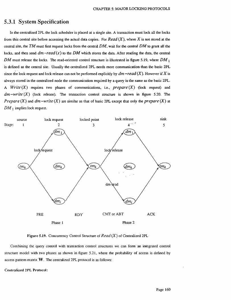
CHAPTER 5: MAJOR LOCKING PROTOCOLS
5.3.1 S ystem Specification
In the centralized 2PL the lock scheduler is placed at a single site. A transaction must lock all the locks
from this central site before accessing the actual data copies. For Read (X ), where X is not stored at the
central site, the TM must first request locks from the central DM, wait for the central D M to grant all the
locks, and then send d m —r e a d ( jt) to the D M which stores the data. A fter reading the data, the central
D M must release the locks. The read-oriented control structure is illustrated in figure 5.19, where D M y
is defined as the central site. Usually the centralized 2PL needs more communication than the basic 2PL
since the lock request and lock release can not be performed explicitly by dm —read (X ). However if X is
always stored in the centralized node the communication required by a query is the same as the basic 2PL.
A Write (X) requires two phases of communications, i.e., prepare (X ) (lock request) and
d m — write (X ) (lock release). The transaction control structure is shown in figure 5.20. The
Prepare (X ) and d m —write (X ) are similar as that of basic 2PL except that only the prepare (X) at
D M i implies lock request.
source lock request locked point lock release sinkStage: 1 2 3 4 " 5
a m dm
lock/request
(ami d m i
PRE RD Y CMT or ABT ACK
Phase 1 Phase 2
Figure 5.19. Concurrency Control Structure of Read (X ) of Centralized 2PL
Combining the query control with transaction control structures we can form an integrated control
structure model with two phases as shown in figure 5.21, where the probability of access is defined by
access pattern matrix W . The centralized 2PL protocol is as follows:
C entralized 2 PL Protocol:

CHAPTER 5: MAJOR LOCKING PROTOCOLS
source lock request locked point lock release sinkStage: 1 2 3 4 5
' m v
lock release dm-write
dm-write
dm-write
(ami Irrii
CMT or ABT ACKPRE RDY
Phase 1 Phase 2
F igure 5.20. Concurrency Control Structure of W ri t e (X ) o f Centralized 2PL
Phase 1:
1.1 The coordinator T M k sends P r e p a r e ( X ) and lock request (PRE) message to all the participants
{DA/;, X e D M i ) .
1.2 The central node DA/; receives the message; and checks for the required locks. If all locks are
granted and it is willing to commit, then it writes the transaction’s record in the log and sends ready
(RDY) answer message to T M k ; otherwise it sends abort (ABT) message to 77V//.. The non-
central DA/; receives the message; and then writes the transaction’s record in the log and sends
RDY to T M k .
Phase 2:
2.1 Upon receiving the answer message RDY or ABT from {DA/;, X eD A Z ;}, T M k sends commit
(CMT) message to all {DA/;, X g D M v } if all o f them have voted RDY, otherwise it writes an
abort record and sends ABT to all {DA/;, X € D A /;}.
2.2 After receiving the command message from T M k , each DA/; writes either an abort or commit
record in log; then executes the transaction and releases the locks; and sends the acknowledge
(ACK) message to T M k .
Page 161
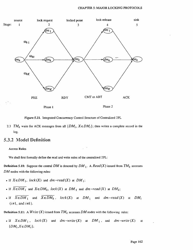
CHAPTER 5: MAJOR LOCKING PROTOCOLS
source lock request locked point lock release sinkStage: 1 2 3 4 5
m !
CMT or ABT ACKRDYPRE
Phase 1 Phase 2
F igure 5.21. Integrated Concurrency Control Structure of Centralized 2PL
2.3 T M k waits for ACK messages from all { D M j , X g D M i }; then writes a complete record in the
log.
5 .3 .2 M odel Defin ition
Access Rules
We shall first formally define the read and write rules of the centralized 2PL:
Definition 5.10: Suppose the central D M is denoted by D M A Read{X) issued from TMk accesses
D M nodes with the following rules:
• If X e D M i , lock(X) and d m - r e a d {X) at D M
• If X e D M i and X g D M k, lock(X) at D M l and d m - r e a d { X ) at D M k\
• If X g D M i and X g D M ^ , lock(X) at D M y and d m - r e a d { X ) at D M t
{ii=-1, and i^k).
Definition 5.11: A Write (X) issued from TMk accesses D M nodes with the following rules:
• If X g D M i , lock(X) and d m —write ( X ) at D M i , and d m — write ( X ) at
[ D M i t X G D M i \ -
Page 162

CHAPTER 5: MAJOR LOCKING PROTOCOLS
• If X e D M i , l o ck (X ) at D M i ,an d d m —write (X) at { D M ; , X e D M i }.
According to the read and write rules o f the centralized 2PL the mean number of accesses generated by
one transaction issued at TMk can be derived by
N acc = i ’P r o b [ r e a d n J C e D M *} (5.57a)
+ 2-Prob {r e a d n X e D M x }
+ N f P r o b {write r \X e D M i }
+ (N f+ l )Prob {w i r t e r \ X e D M i }
Since Prob {read} and Prob [wr i t e ] are independent o f Prob [ X e D M i} , the equation can be
rewritten as
N =i y acc
+
1 -Prob [ X e D M { } + 2 Prob { X e D M i } Prob {r e a d }
N f P r o b { X e D M i } + (Nf+l)-Prob { X e D M i ) Prob {write
Suppose that the probability of a data item being stored in the central node D M is given by
Prob [ X e D M i ) = p dm,
The read-write ratio is previously defined by
Prob {r e a d } = 1 - Y™*
and
Prob {write } = y ^
Substituting Prob { X e D M i }, Prob [ r e a d } and Prob [write } into the equation (5.57a), we have
N =acc NfPdm , + ( N f + 1)(1 -Pdm , )Pdtn , “P 2 ( 1 P d m , )
( 2 Pdm | ) ( Yr w* ) *P (^ V y + 1 —P d m x )Y nvk
= ( N f - 1 ) yni,.k - p drn j + 2
The probabilities o f accessing DMs are defined by the access pattern matrix W as follows.
Theorem 5.12: The access pattern matrix W of the centralized 2PL is given by
Ynv*
(5.57b)

CHAPTER 5: MAJOR LOCKING PROTOCOLS
N r 1 N ,*frwkP d m x( g j ) " P Y n t ' t ( ^ P d m , ) Y r w * ) ( l P d m x ^
( N f 1 ) Y rwk ~ P d m , "P2
( N f ~ 1 )Y rw t ~ P d m , + 2
iVf-1YnvkP d m , ( ^ Pdm \ J £ —\
( N f 1 )Y n v t ~P dm j +2
A ^ - l A^ ( K - N f - l )YnvkPdm [ "P Yrwk ( l ~ P d m l ) f f Yrwk)(^ ~ P d m x ) 1 ) ( X —2 )
C ^ / ^ ) Yrwk ~ P dm j + 2
if 7=1
(5.58a)
if 1
i f 7=1
if 7=^,7^1
if
k = 2 , . . . , K \ J = \ , . . . , K (5.58b)
Proof: According to the read and write rules, the rate of accessing the central node locally is given by
1 P r o b {r e a d } + 1 •P r o b {w r i t e }g>u =
N ,acck
1
N acck
When a transaction is issued from the central node T M [ , we have
coly = Prob {Accesskj | X e D M i n X e D M j } Prob {X e D M j r X e D M j }
+ Prob {A c c e s s kj | X <= D M t r X e D M j } Prob {X e D M t r X e D M j }
0-P r o b {r e a d } + 1 P r o b {w r i t e }
N acckP d m ,
N r \
K - 1
+1 P r o b {R e a d (Xj)} P r o b {r e a d } + I •P r o b { w r i te }
NL acck( 1 P d m , )
N t
K - 1
Since there are copies of a data item X and the probability of reading one o f them is uniformly
distributed,
P r o b {R e a d ( x ;)} =
The equation of COi j can be rewritten as
Page 164

CHAPTER 5: MAJOR LOCKING PROTOCOLS
© j : =Jnvk
N, ~Pdm ]
Nr 1 X - l
Yrwk+ (^~Pdmx )
+
acck (ZCC* X - l
N t
acck
N r - l
K - 1
YrwkP d m x ^ j " ^ Y r w '* ( l P d m t ) ^ j ^ Y rw ^ X ^ P d m x) ^ _ 2
In the case of CD** is given by
cokk = Prob {Accesskk \ X e D M L r X e D M *} Prob {X e D M i r X e DM * 1
+ Prob {Access** |X g D M iH X g D M ^ }Prob { X e D M i r X e D M k }
+ PrcZ> {Access** [ X g D M i ( ~ X e D M k }Prob { X e D M i C X e D M k }
+ Prob {Access kk \ X e D M i r X e D M k }Prob { X e D M i C X e D M k }
0- Prob {r e a d }+1 Prob {wri teN, P dr
acck
N r - 1
K - 1
1 •Prob {r e a d }+1 Prob {write } , , x~Pdm j )
N acck
+ 0
N t
K - 1+ 0
Yrwk
N, P d m xacck
Nf —l
*{r*\’kP dr
K - 1
N r - l
acck
Nt
K - 1
K - 1
Nt~K Pdm | ) K - 1
(N f 1 )Y rw jt Pdm , “ 2
co*y- = P r o b { A c c e s S k j \ X e D M i n X e D M kn X e D M j ) P r o b { X e D M i n X e D M kn X e D M j ) i)
+ Prob {Access kj \ X e D M \ n X g DM * r \X g D M j } P rob { X e D M i n X e D M * n X g D M y }
+ Prob {Access*y | X g D M ^r X e D M kr X e D M j }Prob { X g D M ! n X e D M kr X e D M j }
+ Prob {Access^ | X g D M r X e D M kr X e D M j }Prob { X e D M \ r X e D M kr X e D M j }
0 Prob {r e a d }+1 -Prob {write }
n Z .Pdn
N f - l
K - 1
N r - 2
K —2
0-Prob {read }+ l-Prob {write }+ N Pdm t
1 vacc1 -
N r I
0-Prob {r e a d }+1 •Prob {write }\L~~Pdm, )
K - 1
N t
Nr i
N.acck K - 1
K - 2
Nr I
K - 2
Prob {R e a d (x . ) } Prob {r e a d } + 1 •Prob {write }"* 77 ( \~ P d m x)
I ' n r r
1 -N t
K - 1
Nt
K - 2

CHAPTER 5: MAJOR LOCKING PROTOCOLS
Yru't ( 1 P d m , )
and CO/ty, j & k j ^ l given by
N*
I
N.acck
K - 1
t y - 1
yV/—1
K - 2+ 1 Yrw k ) + Y ’rw k
N ,
( 1 P d m , ) I —N*
K - 1
N,K - 2
*irwkP d m x g j ^“ YrvvtC^ P dm ^ ) ^ ^ Y r H '* X l P d m x ) / j £ _( K - N f - l )
Hence [ ].
If we assume that the central node stores all the data items, i.e. Pdm l = 1, the above equation can be
simplified as
1(/V/—l)Yrw'* + l
"irwkP d m xN j —1
K - 1
[ ( A ^ - o r ^ + i
if 7=1
if 7*1
(5.59)
Arrival Rate Matrix
The queueing network model o f the centralized 2PL can be built in the same way as that of the basic
2PL introduced in chapter 4. The overall structure of the queueing network model is shown in figure 4.2.
Applying the method introduced in chapter 4, the arrival rate matrix and Markov chain matrix of the
queueing network are given by
Aq = M0) ^°> ■ ■ • M P
A-i = y Aj
A,[ CO]^+A,20l>21"K..+A,/£CO/£ i A,i (Oi2~^A,2CL)22~b---+A,^-CO^-2
a 2 = v 7 a 2
A.1 CO +A<203i2^”"-" ‘A. COi A, C02i+A,2C022" ‘--- ”A. '(02
(5.60a)
(5.60b)
• A - 1 G ) u £ + A , 2 C 0 2 £ + . . . + A ^ G ) ^
(5.60c)
A-i 03/ i +A,2 ($k 2+■ • .+A# (£>KK
A 3 = V A 3 (5.60d)
A.1 C O ii-H X 2 0 > 2 i + . . . + ^ 0 0 ^ 1 A,! CD!2 + A,2 0l)22 + . . - + A .^ (£>k 2 ’ ' ' A,[ 6D ]^+ A .2 C D 2£ _K ..+ A .^ C D /£ X
A 4 = V T A 4 (5.60e)
= A.1G>11+A,2G)i2+...+A.K’G)1/r A<i(D2i"l-A,2CD22+---+A. -CD2 * ‘ ‘ A, CDj i -iA,2CD/ 2+ ”-'bA, CDj -
and the communication flow rate matrix is given by
Page 166

CHAPTER 5: MAJOR LOCKING PROTOCOLS
A c = 'Zs = 1
2 A4 (Oj 1
= 2
A^C02i+A«iC0i2
^'1C012+ ^ 2 C021 2X2^>22
X \(O iK + X k ^ K I X2 (£>2K+ \ K (£tK2
and the M arkov chain matrix are given by
P =P '1 0
0 P o
L ocking
Xk <^K2+X 2 (]i>2X
2XK (Ok k
(5.60f)
(5.61)
Locking in the centralized 2PL system is performed at the central node D M 1 . A transaction first
requests locks at D M 1 in the lock request service centre as shown in figure 5.22. A lock request has a
probability 1— q 1 of causing conflict and probability q * of successfully granting a lock. Upon lock
conflict it goes to the blocked queue waiting to be rescheduled; upon granting all the locks, it leaves the
lock request service centre.
Blocking
Lock
Request
jL_
Figure 5.22. Lock Request Service Center at D M \

CHAPTER 5: M AJOR LOCKING PROTOCOLS
We shall still use the method introduced in chapter 4 to calculated the probability o f conflict 1—q j in
the case of fixed waiting conflict resolution .The conflict-avoidance delay at the central model D M j is
defined as the sum for the remaining lock request delay r I2\ls , two way communication delay 2/jl^ and
the transaction execution delays jXe ,
1
\ lb 2 n , \Lt \ le
r 2 1- + — + - (5.62)
where l / |ly is the mean service time to obtain one lock, j l f is the mean service time o f transmission delay
and \±e is the m ean service time of transaction execution.
The probability of conflicts is defined as
mean number o f locks held at node D M \l -<7i =
number o f granules N L ({ock) 2 ) + N L (com 3 ) + N L <£x)
(5.63)
The mean number of locks held at the central node is equal to the sum of the number of locks held by each
transaction multipled by the mean number of transactions in the service centres. The locks held in lock
request stage at D M i are NL^[oclcK From equation (4.55), the total number of locks held at the lock
request centre of D M \ is given by
NL<(ock) = v ■ i
<7i Us '=1
(5.64)
At the communication channels each of the transactions leaving the lock request centre of D M i holds r
locks. The mean number of transactions holding locks at the 2nd and 3rd stage of communication is given
by
KNL\com 21 +NL[com 3) = r t ]T
i=2
a\V _ a® _w n i , + w n i '
(5.65)
At the execution service centre of D M i , denoted by l / t+2» the mean num ber of transactions is given by
n i . Therefore
NL\ex> = r , n . (5.66)
Substituting (5.64), (5.65) and (5.66) into equation (5.63), we have
r '~ l ■ ' K -r— Z'V+MZq l i =i i = 2
_ '
L
r \ n\
(5.67)
Page 168

CHAPTER 5: MAJOR LOCKING PROTOCOLS
T ran sac tio n Execution
For the centralized 2PL only the central node requires specific modification. A transaction will perform
dm —r e a d (X ) or d m —write (X ) at the central node if the data item X is stored in D M i ; otherwise a
transaction only performs locking at the central node. Since Prob { X g D M i } = p j m J , the actual
arrival rate of the transaction execution centre at D M i is reduced to
N eXl^1jc+2 ” w ^ 1a:+2 (5.68)
Lyacc
D iffusion A pproxim ation Q ueueing Network
Applying the diffusion approximation method introduced in section 4.4, various mean measurements
can be obtained. Therefore q [ can be solved numerically. The relative throughput at service centre i is
given by
m= P 0 i + £ e j P j i 0 = 1 . •• • > m ) (5.69)
;= i
where
m = K ( K + 2)
The arrival rate of service centre i is proportional to the relative throughput.
Xj = (5.70)
The utilization of the service centre i is
X^eiPi = --------- , i f XoeiK^i (z = l , . . . ,m) (5.71)
bl
u n d e r the condition of heavy traffic, the total number of arrivals to station / in the interval [ 0 ] will
be normally distributed with mean X t f and variance
mX [ ( C j - 1 ) p j i + 1 \ X j P j i t ( i = 1 , . . . ,m ) (5.72)
j = o
By constructing the diffusion approximation to the length of individual queue, where is the
density function approximating the length of the i-th queue, the stationary solution of the diffusion
approximation equation is given by
Page 169

CHAPTER 5: MAJOR LOCKING PROTOCOLS
T,>1
p , ( l - e Y"''), 0 < x , < l
where
Yi = - 2 p i / a l-
The parameters of the above equations are given as,
P . = K - Him
a i = p i \i iK j + £ l ( C j - l ) p j i + l ] X j p j i >=o
(5.73)
(5.74)
(5.75)
The squared coefficient of variation of the interarrival time C ,, ( /= 1 , ' ' ' , m ) can be obtained
numerically by solving a system of linear equations
( 1 - p i )£ ( C j - l ) X j P } = l - ( l - p i ) p u
( / = ! , . . . ,m ) (5.76)
where K t is the squared coefficient of variation o f the service time distribution at service centre i.
The approximate average queue length is
r a,-Hi = Pi 1 - 2 P i
(5.77)
The lock request service centre at the central node l/^+ i in figure 4.5 is an IS service centre which can
be represented by a single server service centre with service capacity equal to 1 I N i |4 i;c+1. The
throughput o f lock request service centre l ^ + i is defined as
p i - X \ I N 1 Jlir 1AT+l 1AT+1 (5.78)
where N ]_ is given by equation (4.113) and rewritten as
2 X U
Ijfl + + 1) (5.79)
C i is the squared coefficient of the variation of the interarrival time at service centre which
equals to the sum of the independent variance jof the interdeparture time of all the other service centres to
centre
Page 170

CHAPTER 5: MAJOR LOCKING PROTOCOLS
1 mC l*+i = nj 2 t ( Q ” 1)P« 1at+i + 1 y^iPi ljf+i (5.80)
lff+i i=0
The mean throughput o f the lock request centre at the central node P i^ , the squared coefficient C f\ and
the mean queueing length tij ( / = l , . . . , m ; k = l , . . . , K ) can be respectively obtained from equation (5.78),
(5.76) and (5.77).
Applying Little’s law, the average turn-around time o f the system is
™ HiTa ~ £ T (5.81)
r = l A<>
5 .3 .3 P er form an ce R esults
The parameters o f the evaluation of the centralized 2PL system are the same as basic 2PL. They are
given in tables 4.3 to 4.8.
The overall system performance is given in terms of m ean turnaround time o f the system. The effect of
different parameters towards the mean response time is studied. Results of centralized 2PL are given in
figures 5.23 to 5.27.
Read-Write Ratio
Figure 5.23 illustrates the system behavior affected by the read-write ratio Its parameters are
given in table 4.4. It can be clearly seen that under y n v= 0 .2 the response time increases much more
slowly than that in other cases.
Data Replication
The response times under different mean number o f duplicated copies are given in figure 5.24. The
parameters are given in table 4.5. The response time of the system increases as /Vy increases. The results
show the same pattern as that in other cases except majority consensus. We can also find out that the
system with no replication performs much better than others.
Lock Granularity
Figure 5.25 shows the effect of database granularity with parameters given in table 4.6. The mean
number of locks for each transaction vs. the total number of granulars is set at 5 /5 0 0 , 1 5 /1 5 0 0 ,
2 5 /2 5 0 0 , 3 5 /3 5 0 0 respectively. The results suggest that the difference between coarse and fine
granularity is the smallest among all the 2PL algorithms, because the locking is performed only at the
central node.
R ead-W rite Ratio vs. Data Replication
Page 171

CHAPTER 5: MAJOR LOCKING PROTOCOLS
Response
Time
(in seconds)
0.40.6
5 -
1.50 1Interanival Rate
Response
Time
(in seconds)
Figure 5.23. Response Times with Different Read-Write Ratio Yrw
6
5
4
3
?
1
-0 .5 I 1.5Interarrival Rate Xq
Figure 5.24. Response Time with Different Replicated Copies N f
Page 172

CHAPTER 5: MAJOR LOCKING PROTOCOLS
Response
Time
(in seconds)
Response
Time
(in seconds)
6
5
4
3
2
1
■0 I5Interarrival Rate
F igure 5.25. Response Times with Different Granularity r ! L
0.75,
4 -
2 -
o 3 4Mean Number of Replicated Copies /Vy
Figure 5.26. Response Times vs N f with Different Read-Write Ratio Yrw
Page 173

CHAPTER 5: MAJOR LOCKING PROTOCOLS
0.0006
0.0004
Mean
Conflict
Rate p c
0.0002
20 2510 155M ean Number of Locks r
F igure 5.27. Mean Conflict Rates with Different Replicated Copies N f
Figure 5.26 shows the change of response time with N f under different y,w The response time at the
starting pionts, i.e. N f = l , for the centralized 2PL is relatively smaller than that in other cases. This is
because centralized 2PL protocol causes less blocking than other protocols. In the cases of low read-write
ratio 7™-—0 and 0 .2 5 , the response times tend to decrease for y ^ = 0 and almost hold at the same
level for 7 ^ = 0 .2 5 . The centralized system is clearly in favor of read oriented transactions.
Conflict Rate
The centralized 2PL algorithm causes much less locking conflicts than any other algorithm as shown in
figure 5.27. it is also interesting to notice that the data replication does not affect conflict rates very much
as opposed to the other 2PL algorithms. This is because that locking is performed not only at the same data
copy but also at the same site. We can conclude from all the 2PL algorithms studied that the wider the
locking operations are spread, the higher the locking conflict rates are. Figure 5.27 indicates how the
number of duplicated copies N f effects the conflict rate of lock request. The higher the N f , the greater the
conflict rate p c . So N j should be carefully chosen to obtain a good system performance. The parameters
are given in table 4.8. There exists a thrash at 0 < r < 4 under N f= 1, which means that the mean conflict
rate decreases as the mean number of required locks increases. It is likely caused by the error in numerical
convergence when solving small q in equation (5.67). However the numerical method used here gives us
satisfactory results in almost all the other cases.
Page 174
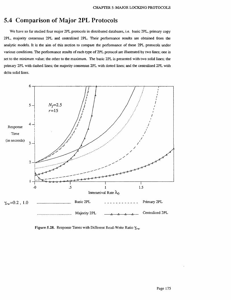
CHAPTER 5: MAJOR LOCKING PROTOCOLS
5.4 Comparison of Major 2PL Protocols
We have so far studied four major 2PL protocols in distributed databases, i.e. basic 2PL, primary copy
2PL, majority consensus 2PL and centralized 2PL. Their performance results tire obtained from the
analytic models. It is the aim of this section to compare the performance of these 2PL protocols under
various conditions. The performance results of each type o f 2PL protocol are illustrated by two lines; one is
set to the minimum value; the other to the maximum. The basic 2PL is presented with two solid lines; the
primary 2PL with dashed lines; the majority consensus 2PL with dotted lines; and the centralized 2PL with
delta solid lines.
Response
Time
(in seconds)
6
5
4
3
1
■0 .5 1.51
'^ ,= 0 .2 , 1.0
Interarrival Rate Xq
Basic 2PL _________
Majority 2PL -A A A A -
Primary 2PL
Centralized 2PL
Figure 5.28. Response Times with Different Read-Write Ratio y r

CHAPTER 5: MAJOR LOCKING PROTOCOLS
Response
Time
(in seconds)
6
5
4
3
?
1
.5 1 1.5Interarrival Rate Xq
Figure 5.29. Response Time with Different Replicated Copies N f = l , 4
Response
Time
(in seconds)
6
4
3
?
0 .5 1Interarrival Rate
Figure 5.30. Response Times with Different Granularity r /L = 5 /5 0 0 , 35 /3500
Page 176

CHAPTER 5: MAJOR LOCKING PROTOCOLS
Response
Time
(in seconds)
Mean
Conflict
Rate p c
4 -
2 _
? 3 41Mean Number of Replicated Copies N f
Figure 5 3 1 . Response Times vs N f with Different Read-Write Ratio 7 ^ = 0 ,1
0.08
0.06
0.04
0.02
■0
10 25205 15Mean Number of Locks r
F igure 5 3 2 . Mean Conflict Rate with Different N f — I , 3
Page 177

CHAPTER 5: MAJOR LOCKING PROTOCOLS
Read-Write Ratio
The results shown in figure 5.28 indicate that the centralized 2P1 performs best, the primary 2PL is
better than the majority 2PL and the basic 2PL has the worst performance. At the extreme case, i.e.
yrw= I.O , the primary, majority consensus and basic 2PL perform nearly the same, while centralized 2PL
is still much better than the re s t
Data Replication
Figure 5.29 illustrates the performance curves with different replicated copies. The best result occurs
under N f = \ with centralized 2PL. At low A o (X o < 0 .6 ) the response times of the centralized and primary
2PL under N f = 4 are smaller than those o f the basic, primary and majority 2PL under N f = l . But at higher
X q (X o > 0 .6 ), the situation becomes the opposite. The performances of the basic and primary 2PL under
N f ~ 4 are the worst among all the cases. The response times increase dramatically as interarrival rate
approaches 0 .7 .
Lock Granularity
The effect o f different lock granularities are shown in figure 5.30. Again centralized 2PL outperforms
the rest. The performance can be graded in the following order, centralized 2PL first, majority consensus
2PL second, primary 2PL third and basic 2PL fourth. Centralized 2PL is least affected by the lock
granularity, while basic 2PL is most affected.
Read-write Ratio vs Data Replication
Figure 5.31 illustrates the effect o f read-write ratio vs data replication. Under read only case, i.e.
Ym'=0, the response time decreases as the mean number of replicated copies increase in the centralized
2PL, majority consensus 2PL and primary copy 2PL. W hile for basic 2PL, it almost holds at the same level.
Under write only case, i.e. y'nv= i , the basic 2PL, primary 2PL and majority consensus 2PL perform almost
equally badly, while the centralized 2PL again outperforms the rest. The performance can be graded as the
centralized 2PL first, majority consensus 2PL second, primary copy 2PL third and basic 2PL fourth.
Conflict Rate
The mean conflict rates of the four 2PL protocols are presented in figure 5.32, in which centralized 2P1
almost has no conflict rate. The majority 2PL and basic 2PL have higher but similar conflict reates. The
range of conflict rates in the primary 2PL is significantly greater than the rest 2PL protocols. Especially
under N f= 3 , the conflict reate o f the primary' 2PL is much higher than the rest.
Generally speaking, centralized 2PL outperforms the other 2PL algorithms under the test condition. It is
interesting to notice that the locking conflict rate is strongly associated with the distribution of the locking
activities. The wider the locking activities spread, the higher the conflict rates are. Another interesting
finding is that the degree of data replication has a big impact on the response time. By properly choosing
Page 178

CHAPTER 5: MAJOR LOCKING PROTOCOLS
the parameter, optimal performance can be obtained The finding of lock granularity being less effective to
the overall performance is not surprising, since the lock overhead in the test system is quite small. These
performance results are useful in comparing various concurrency control algorithms and designing
distributed database systems.
5.5 Summary
In this chapter, the modeling method introduced in chapter 4 is consistently extended to model primary
2PL, majority consensus 2PL and centralized 2PL protocols. The analytic model is proven to be applicable
to a wide range of distributed database protocols, especially 2PL. Many useful findings are obtained by
comparing the evaluation results o f these 2PL protocols.
Page 179

Chapter 6. Empirical Evaluation of an Actual DDB
In the previous chapters, analytic models of distributed database systems have been introduced and
validated by various simulation models. However it will be more convincing if the analytic model
can be validated against an actual distributed database system. In this chapter, we shall present an
implementation o f a prototype distributed database system and measure the real system to validate the
analytic model.
6.1 Introduction
Various distributed database systems have been designed and implemented in recent years8. Most o f
them employ point-to-point communication and static distributed database configuration. With the
availability of the multicast communication facilities from the 4.3BSD UNIX kernel, efficient, robust and
reliable distributed databases can be built. In this chapter we introduce a prototype distributed database
system called the Distributed Robust File Store (DRFS) which is designed to manage replicated copies o f
data, and to provide consistent and concurrent access to the data. The reason for calling it a file store rather
than a database is that we only concentrate on studying the concurrency control algorithm while
simplifying the database interface language. The nature of the multicast protocol enables the system to
achieve greater parallelism and thus high performance. High robustness is obtained by the introduction of
dynamic configuration of transaction managers. Furthermore novel failure recovery algorithms are used to
maintain the reliability of the system. The performance of the implemented system is measured in terms of
the throughput and utilization of the system under different work loads. The measurement results are
compared with the analytic results.
The sections in this chapter are organized as follows: section 2 describes the architecture of the system;
section 3 introduces the algorithms and techniques used to manage the dynamic configuration o f the
transaction manager group; section 4 gives the concurrency control mechanisms and implementation
details of transaction management; section 5 discusses the failure recovery algorithm and its
implementation; section 6 presents the analytic model of the distributed database system built on an
Ethernet; section 7 compares the measurement results with the analytic results obtained by mathematic
modeling. Due to limited space in the thesis, implementation details of the DRFS system can be found in
the references60,50,56,5 ’5*’58,59,52,53
6.2 Architecture
6.2.1 G en era l A rch itectu re
The DRFS, as shown in figure 6.1, consists of three modules - the Transaction Manager (TM), the
Data Manager (DM) and the Multicast Network (McNet). The Transaction Managers (TMs) control the

CHAPTER 6: EM PIRICAL EVALUATION
DBDMDM TMDB
McNet
DM DBTMTM
Figure 6.1. Architecture of the DRFS
distributed execution of transactions ori^user’s behalf. They provide access interface for users and control
concurrent transaction execution. The DRFS system maintains a dynamic configuration of all the active
TMs by storing the current status o f all the TMs at each TM site. A TM also contains the global schema
of the data stored in the system, which records the names and number of copies o f the files in the DRFS.
All data managed by the DRFS are stored by Data Managers (DMs). The DMs manage local data
manipulations under the supervision of TMs. All the data controlled by the TM s have to be consistent.
The communication between the TMs and DMs is via a Multicast Network (McNet). The McNet is a
multicast communication interface which provides the following services:
• atomic transaction control, which means that an update transaction is either done at all DMs or not at
all;
• TMs group management, which maintains a dynamic configuration of the group o f all the active TMs.
Page 181
CHAPTER 6: EMPIRICAL EVALUATION
• failure recovery and retransmission, which guarantees that network failures will be recovered and no
inconsistent state will be left after recovery.
6 .2 .2 P hysica l A rch itectu re
The physical structure o f DRFS is illustrated in figure 6.2. The system is built on a number o f Sun
workstations connected by an Ethernet local area network. The Sun workstation is a host computer which
can be accessed from both the console and remote terminals. Some o f the Sun workstations have file stores
m anaged by local DMs. Others are simple workstations without their own file storage. The DMs are
always built at the workstations with their own storage while TMs can be built on any types of
workstations.
The Ethernet is a broadcast baseband local area network. It uses a carrier sense multiple access
(CSMA) protocol to control transmissions and avoid collisions at the physical and link layer of the OSI
reference model. The nature of Ethernet enables a broadcast type communications, which has the
advantage of transmitting K messages at the cost o f one. With the further development o f interprocess
communication protocols at network and transport layer, a new communication primitive called multicast
is made available in 4.3 BSD UNIX system. Multicast is simultaneous transmission o f data, rather like
broadcast, but to a restricted and well defined set of destinations. It is a desirable communication primitive
for the applications requiring communications between a group o f processes.
6.2 .3 A ccess S tru c tu re
Figure 6.3 illustrates the types of accesses to DRFS from a user. A user can only contact a TM which
manipulates distributed replicated data copies. The types of the DRFS operations that a user can issue are
Create, Delete, Open and Close files and Read and Write records. Consider a transaction involving
creating three copies of a file in DRFS. A user first issues a Create_File command to a TM. Upon receiving
a user request the TM coordinates a concurrency control protocol with a set o f DMs to perform the
distributed file creation transaction. Once a DM receives the file creation request from the TM , it performs
locking and local file creation operations under the control of the coordinating TM. The DMs always sit
there waiting for calls from a TM. It serves as an interface between file systems and the TMs. On one hand
it acts as a participant of a concurrency control protocol with the coordinating TM. On the other hand it
controls the file system to perform the required local file operations.
6 .2 .4 P rogram S tru c tu re
This DRFS architecture, shown in figure 6.4, gives a clearly layered programming structure with user at
the top level, TM at the second level, DM at the third level and the actual files at the bottom level. The
advantage of the clearly layered structure is to achieve efficiency and transparency. The efficiency lies on
the fact that functions of programs at different levels can be modified easily and extended without affecting
programs at other levels. The data transparency is achieved using automatic control o f the data allocation
Page 182

CHAPTER 6: EMPIRICAL EVALUATION
File
Name Server
File Server
Multicast
File Server
Multicast
Ethernet
Multicast
Name Server
Multicast
Name Server
Multic ast
Su
File S er
n
ver
T T T T T T T T T TFile
Figure 6.2. The Physical Structure of the DRFS
by the TM. The user needs only to provide the number of replicated copies that he/she wishes to distribute.
The TM then chooses the actual locations of the copies for the user.
The TM processes are started by triggering the TM group management protocol to join the TM group.
This joining operation is done once for all during the life time of a TM. Once a TM becomes an active
member o f the TM group, it keeps listening to user requests. When a user request is received, a TM
controls the distributed execution of the transaction with the participation of a number of DMs. There are
Page 183

CHAPTER 6: EMPIRICAL EVALUATION
User DMTMFile
DMFile
User TM
User TM
DMFile
Figure 6.3. Access Pattern of the DRFS
two multicast groups: the TM group with address (tm_group), which supports communication within the
TM group, and the TM-DM group with address (dm_group), which is for communication between TM s
and DMs.
6.3 Dynamic Configuration of the TM Group4
In conventional distributed databases, the configuration of TMs is static. This approach, however,
makes the extension of a system difficult and reduces its reliability. In order to enhance the robustness o f a
distributed system we introduce a technique to maintain a dynamic configuration of the TM group. This
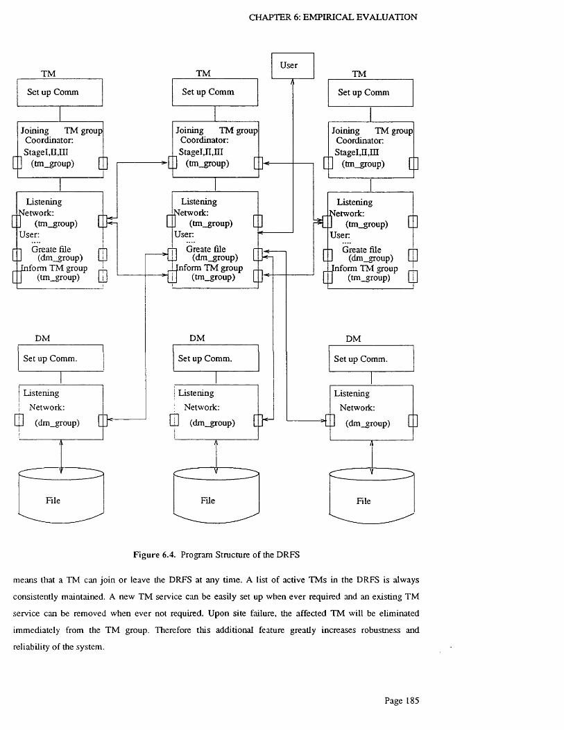
CHAPTER 6: EMPIRICAL EVALUATION
TM
Set up Comm
Joining TM group Coordinator: StageI,H,III
Q] (tm_group) Q]
[ f
Listening etwork:
(tm_group) User:
$[ f
DM
Set up Comm.
Listening
□Network:
(dm_group)
ft
File
Greate file (dm_group)
form TM group * (tm_group) Lll
Q h
•[]
TM
Set up Comm
Joining TM group Coordinator: StageI,II,m
(tm_group)
ofListening etwork:
(tm_group) User:
r- 1 Greate file n_ij (dm_group)
ilnform TM group n H (tm_group)
DM
Set up Comm.
Listening
Network:
] (dm_group)
File
[]
[ ]
[]=Ch
O H
User
[]
TM
Set up Comm
Joining TM group Coordinator: Stagel,n,m
(tm_group) [I]
krListeningetwork:
(tm_group) User.
[ ]
r
DM
Set up Comm.
Listening
Network:
(dm_group)
File
[]
r aGreate file
(dm group) form TM group p ,
(tm _group) [JJ
[ ]
Figure 6.4. Program Structure of the DRFS
means that a TNI can join or leave the DRFS at any time. A list o f active TMs in the DRFS is always
consistently maintained. A new TM service can be easily set up when ever required and an existing TM
service can be removed when ever not required. Upon site failure, the affected TM will be eliminated
immediately from the TM group. Therefore this additional feature greatly increases robustness and
reliability of the system.
Page 185

CHAPTER 6: EMPIRICAL EVALUATION
6.3.1 G rou p {M anagement P rotocols
Three protocols are used to manage the dynamic configuration of the TM. Protocol P I involves
obtaining the dynamic configuration o f TMs; protocol P2 propagates the modified configuration to all the
existing TM s and protocol P3 obtains the global data schema for the new TM . Setting up a new TM
requires all three protocols (P I, P2 and P3), since the new TM must first acquire the current status o f the
existing TM group, then adds itself to the group, controls the propagation of the modified configuration to
other TM s and finally obtains the global data schema to provide data m anagem ent service to users.
Deleting a TM obviously requires only protocol P2.
The algorithms of protocol P i , P2 and P3 are as follows:
Protocol P I : Get TM Group Membership List
New TM:
• multicasts HELLO to the address of the TM group.
Existing TMs:
• receive the request and send back a copy o f the membership list of TMs with command
MLIS_RESP. This ensures that even if only one TM responds to the request, the new TM
will have full knowledge of the group membership.
New TM:
• waits for reply from the existing TMs.
— If no answer is received when timeout, repeat the whole procedure;
— If there are more than three time-outs, the new TM sets up an empty global data schema;
— Otherwise at least one reply is received and the protocol is successfully completed.
Protocol P2: Join (/Leave) TM Group
Phase 1:
New TM:
• multicasts ADD_ME to the TM group (tm_group).
Existing TMs:
• receive the message and check the accuracy of Membeiiist. If it is correct, set up a
pre-write of the new list and acknowledge the receipt of the request with OK. The pre
write is used to detect conflict.
Phase 2:

CHAPTER 6: EM PIRICAL EVALUATION
New TM:
• collects replies from existing TMs.
— If the new server has got a positive reply from everybody, it multicasts COMMIT.
— If one of the replies is SORRY, the sender multicasts ABORT.
— Otherwise it re-transmits the request until all known group members have
responded or, eventually, it times out and assumes that the missing ones failed. It is
then allowed to proceed with the remaining group members.
Existing TMs:
• wait for replies from the new TM.
— those who get the COMMIT message delete the pre-write list, update the
membership list and acknowledge the request (ACK).
— those who get an ABORT message only delete the pre-write list and acknowledge
the request (ACK).
New TM:
• has to collect ACKs and retransmit until either it has all o f them or (at long last) has to
assume failure of the missing ones. If the transaction has to be aborted, it will restart
from protocol P I. If all acknowledgements are collected, it multicasts an
acknowledgement to the receivers.
Existing TMs:
• listen to the sender’s acknowledgement. If they are not received before timeout, a
failure recovery procedure has to be trigged.
Protocol 3: Get Global Data Schema
New TM:
• selects an existing TM from the membership list and unicasts a FLOP_REQ to the selected
TM to obtain a global data schema.
Selected TM:
• Upon receiving the FLOP_REQ, the selected TM sends back a copy of the global data
schema.
New TM:
• If the new TM receives the global data schema within a given time the protocol is terminated;
otherwise it repeats the procedure starting from step 1.
Page 187

CHAPTER 6: EMPIRICAL EVALUATION
6.3 .2 P rotoco l Im p lem en ta tion
Protocol P I and P3 are one phase protocols and P2 is a modified basic two phase commit protocol.
Protocol P I is coded in subroutine get_memlist() at the coordinator TM and subroutine listenall() at the
participant TM; protocol P2 is built in subroutine update_mem() and listenall() and protocol P3 is in
get_nslist() and listenall() respectively. Part of the functions performed by listenall() procedure is to listen
to the network (tm_group) address. It acts as a participant TM to respond the request from a coordinating
TM in protocol P I, P2 and P3 introduced above. It responds to the coordinating TM ’s HELLO w ith
M LSTJRESP, ADD_ME with OK/SORRY, DEL_ME w ith OK/SORRY, COMMIT with ACK, ABORT
with ACK and FLOP_REQ with FLOP_RESP.
In protocol P2 a version-numbering technique has been used to improve the efficiency of the protocol.
Each version o f the membership list o f the TM group is marked with a version number. All the copies o f
the membership list stored at different TMs have the same version number. The version number is updated
consistently in all the TM s whenever there is a change of membership in the TM group. This technique
enables the protocol to transmit and update only the version number rather than the entire membership list.
Another technique used in P2 is to use prewrite to control locking. At the first phase of P2 a prewrite is
used to reserve the right to exclusively use the memberlist for updating. This is done by increasing the
version number of the memberlist by one. For example, suppose TM , and T M j both want to leave the
DRFS w hen the version number of membership list is n. Suppose T M [ triggers the protocol P2 first. The
version numbers at all the TMs are then checked and increased to (n + 1 ). Suppose T M j triggers P2 when
its version number is still n. T M j then checks its version number with other T M ’s version number. It is
obvious that some conflicts will occur therefore T M j ’s update will be rejected.
6.4 Transaction Management
The transaction management deals with the actual distributed data manipulation at the record and file
levels. The consistency of the DRFS is maintained by the transaction management protocols. Each
transaction is executed as an atomic operation, which means that it is either done completely or not at all.
The granularibf lock in the DRFS is record. On the physical file each record is associated with a lock field.tiu
Locking is physically performed by setting or resetting the lock field of a record.
6.4.1 T ra n sa ctio n [Management P rotoco l
A transaction is executed between a TM as the coordinator and a set o f DMs as the participants. In
order to achieve robustness of the system, we employ a majority consensus two phase commit protocol.
Record update is propagated to a majority of the DMs holding the record. Reading a record involves
asking all o f the DMs to send the record w ith'its time stamps and select a most up to date copy from a
majority of the replicated records.
Page 188

CHAPTER 6: EMPIRICAL EVALUATION
Protocol P4: Majority Consensus 2PL
Phase I:
Coordinator (TM):
• Issue an atomic transaction.
• Multicast the transactions to the participants in (dm_group).
Participants (DMs):
• Wait for a transaction.
• Receive a transaction.
• Try to lock.
— If locks are granted, send OK to the coordinator.
— If locks are not granted, send SORRY to the coordinator.
Phase II:
Coordinator (TM):
• Waits for Answer messages.
— If a majority of OK messages are received, it multicasts COMMIT to the
participants in (dm_group).
— If less then a majority of OK messages are received at time-out or a SORRY
message is received, multicast ABORT to all participants in (rm_group).
• Waits for ACK messages from the participants.
Participants (DMs):
• Wait for command message.
— If command is COMMIT, execute the transaction and release locks.
— If command is ABORT, release locks.
• send ACK to the coordinator.
Coordinator(TM):
• waits for ACK responses
— If a majority of ACK messages are received, complete the protocol.
— otherwise trigger recovery protocol.
6 .4 .2 P rotocol Im p lem en ta tion
Protocol P4 is designed to deal with data manipulation transactions, such as Create, Delete, Open,
Close, Read and Write, under user’s request.
Page 189
CHAPTER 6: EM PIRICAL EVALUATION
A user’s request is picked up by the listenall() procedure. Once a user’s request is picked up, the TM
will start to coordinate a transaction with a group of DMs by calling RFCreate(), RFDelete(), RFOpen(),
RFClose(), RRReadO, and RRWrite() accordingly.
In each TM, a global data schema is stored in its stable storage. The global data schema is updated and
kept consistent at all the TMs upon file creation and deletion operations.
Since only DMs store the actual data of the DRFS, it must keep a list o f the local data files stored in
them. W e call this list the local data schema in contrast to the global data schema stored in TMs. The local
data schema, which contains the names and locks of the data stored in each DM, is stored in the stable
storage. M oreover it also keeps a dynamic open-file-table in the main memory to record the status o f the
files used at run time.
The protocol is implemented in procedure Phasel_maj() and PhaseII_maj(). Phasel_maj() procedure
performs the first phase o f protocol P2 from the coordinator node. It tries to enforce all the participants to
take part in the transaction. Those who store the data will respond. At the end of the first phase, a list o f
DMs, which have responded, is recorded in a vector (testmem). The vector (testmem) is then packed into
the multicast COMMIT or ABORT message and sent to all the DMs in the second phase. Upon receiving
the message, the DM will first check the name list. If the D M ’s own name is found in the list, it either
COMMITS or ABORTs and then sends an ACK; otherwise it simply clears the transaction and does not
send ACK.
The PhaseII_majO procedure performs the second phase of two phase commit protocol from the
coordinator node. It multicasts either COMMIT or ABORT according to the status passed from the first
phase (phasel). It requires all the previously responded DMs to either COMMIT or ABORT the
transaction. The name list o f the previously responded DMs is packed in and sent with the COMMIT or
ABORT command to (dm_group) to enable those particular DMs to participate in the transaction.
A listen() procedure is used to enable the DMs to respond to the T M ’s request. It acts as the participant
o f the file manipulation transaction in protocol P4. In the first phase of the transaction, the DM receives a
CREAT_F, DEL_F, OPEN_F, CLOSE_F, READ_F, or WRITE_F request from a TM. It then performs
required locks at the physical level by calling PREFS_tcreate(), PREFS_fdelete(), PREFS_fopen(),
PREFS_fclose(), PREFS_rread(), or PREFS_rwrite() accordingly. In the second phase, the DM receives
either a COMMIT or ABORT from the TM. It then executes the transaction by calling FS_fcreate(),
FS_fdelete(), FS_fopen(), FS_fclose(), FS_rread(), or FS_rwrite() accordingly. The correct match between
the messages received in the first and second phases is maintained by a buffer manager. The message
received in the first phase is put into the buffer with its transaction id. The COMMIT or ABORT message
received in the second phase is checked against the transaction id in the buffer. If it is matched, the DM
will execute the transaction according to the content o f the message buffered in the first phase; otherwise it
simply throws away the message. At the end of the execution, the message is deleted from the buffer.
Page 190

CHAPTER 6: EMPIRICAL EVALUATION
6 .4 .3 P rotocol to U p d a te G lobal D a ta S ch em a
Since the file creation and deletion transactions change the content o f the global data schema stored at
all the TMs, it is necessary to propagate the change to all the TM s by using protocol P5. A TM first gets
the file creation or deletion command from user, and then acts as a coordinator o f the update transaction
while other TM s act as the participants. We use a special one and half phase protocol to execute the
propagation. Crash recovery algorithms are used in the protocol to cope with either coordinator failure or
participant failure.
P rotocol P5 Update Global Data Schema
Phase 1:
Coordinator (TM):
• sends CREATE_F or DEL_F command to all the other participant TMs.
Participants (TMs):
• Upon receiving the CREAT_F or DEL_F message, each participant updates its own
global data schema by calling upd_flop() or delete_in_flop() and replies with an ACK.
Phase 2:
Coordinator (TM):
• receives the ACKs and records the name of the acknowledged participant.
• If all the ACKs from the participant TMs are received, it multicasts a further
FLOP_ACK to all the TMs; otherwise it passes the name list of the participants who
did not reply; and triggers the recover protocol.
Participants (TMs):
• wait for FLOP_ACK from the coordinator. If the FLOP_ACK is correctly received the
protocol is terminated; otherwise a recovery protocol will be triggered.
6.5 Failure Recovery
The robustness of the DRFS system lies on its ability to cope with unexpected failures such as network
failure, host failure and process failure. These failures can happen at any stage of a transaction. It can cause
either the coordinator or the participant o f a transaction to fail. A two phase commit protocol is widely
admitted as not being resilient to network failures especially to coordinator crash. The recovery' procedures
are designed to cope with this problem.
The recovery procedures are used recursively in all stages of protocols. To collect K responses, a
checkup vector is set up to record the number and names of the receivers. If the number of responses is less
than K, the recovery procedures will be triggered. It retransmits the previous command and recursively
Page 191

CHAPTER 6: EM PIRICAL EVALUATION
collect the K required responses until succeeds.
6.5 .1 P artic ip an t F a ilu re R ecovery
Protocol P2 is used w henever there is a new TM joining or an old one leaving, the member list o f the
existing TM has to be changed. However, various failures can occur during the execution o f the protocol.
During the first phase o f protocol P2, the coordinating TM sends ADD_ME or DEL_M E to all the
participant TM in the member list. Upon receiving the message from coordinator each participant replies
OK to the coordinator. The coordinator is supposed to collect all the answers from the participants. I f one
or more participants fail to reply when time out, the coordinator then sends a ABORT message to all the
participants to abort the transaction. So that no inconsistent updates can ever happen at this stage. The
coordinator will restart the transaction after a random wait.
During the second phase o f protocol P2, the coordinator sends either COMMIT or ABORT to all the
active participants. Upon receiving the message each participant will response with an ACK. The
coordinator is then expecting the ACKs from all the participants. It records the names of the participants
who have replied with a ACK. I f any failure takes place during this stage, the coordinator will be unable to
receive all the ACKs, in which case the recovery protocol will be triggered to restore the system to a
consistent and correct state. It should be noted that after the coordinator sends COMMIT message, there is
no other way but to continue the transaction w ith the current state. Therefore the recovery protocol tries to
delete the failed participant from the active member list and informs all the active TMs about the
membership modification.
6 .5 .2 C o o rd in a to r F a ilu re R eco very
The coordinator failure recovery is the most difficult problem associated with the two phase commit
protocol. Here we use a novel method in P2 and P4 to deal with this problem. There are two cases we have
to deal with. One is the failure during the first phase o f two phase commit protocol, the other is the failure
at the second phase.
If the coordinator fails at the first phase of P2 after sending the ADD_ME or DEL_ME message to all
the participants, it is the responsibility of the participants to trigger the recovery process. Upon receiving
ADD_M E or DEL_ME, each participant sets a random time out to monitor the coordinator. If it does not
receive any COMMIT or ABORT from the coordinator when time out, it triggers the recovery protocol.
Therefore the coordinating TNI is deleted from the member list after recover. Upon receiving the recovery
message, the rest of the participants removes the monitoring time out.
We shall now consider the case in which the coordinator fails at the second phase after sending
COM M IT or ABORT to all participants. If all the participants have received the COMMIT or ABORT
message, the transaction is propagated correcdy anyway. The failure of the coordinator will then be
detected by the next arriving transaction. If somehow one or more participants have not received the
Page 192

CHAPTER 6: EMPIRICAL EVALUATION
COM M IT or ABORT when time out, it will trigger the recovery process in just the same way as it does in
the first phase recovery.
6 .5 .3 R ecovery P rotoco l
The recovery protocol mainly performs two tasks, to confirm the status of the failed TM and to delete
it from the member list.
P ro toco l P6: Failure Recovery
Coordinator:
• Unicast YOU_DEAD? to the failed node;
Participant:
• If busy, send BUSYF; otherwise send ALIVE;
Coordinator:
• waits for reply from the failed node.
— If an ALIVE is received, continue from where it stopped.
— If a BUSYF is received, wait for a random period of time and continues from where it
stopped.
— Otherwise restart from the beginning.
— If no answer is receive after sending YOU_DEAD? for three times, delete the crashed
TM from membership list.
— Multicast DEL_FNS with the reduced membership list to the TM group (tm group);
— Collect all the ACKs from TMs. (*The recover procedure is called recursively if there
is a failure at this stage.)
The protocol is implemented in procedure recoverf) for participant failures and cor_recover() for
coordinator failures. The name list o f the failed servers is passed as a parameter to the recovery
procedure. A checking message called "YOU_DEAD?" is first sent to the failed server to check the failure.
If there is no reply after three time out, the failure is confirmed. The failed server is then deleted from the
member list. The notification o f the failure is propagated to all the TMs by sending a DEL_FNS message
and collecting all the ACKs.
It should be noted that failures could happen inside the recover)’ procedure. Therefore the recovery
protocol is used recursively.
Page 193

CHAPTER 6: EMPIRICAL EVALUATION
6.6 Analytic Model of the DRFS
6.6.1 A n a ly tic iVIodel o f the E th ern et
Ethernet is a local area bus network which employs carrier sense multiple access (CSMA) technique20.
We shall first introduce the modeling method for general broadcast networks and then apply the method to
a specific bus network, i.e. Ethernet. Two most popular broadcast protocols are pure ALOHA and slotted
ALOHA.
P u re A L O H A
The basic idea of pure ALOHA protocol is very simple1. A user can transmit a packet at any time
without any sensing or synchronization. If it receives the packet correctly, the transmission is successful;
otherwise a collision is assumed to occur during the packet transmission period and the packet has to be
retransmitted. The retransmission is followed by a random delay to avoid further collision
Let us consider a packet transmission using a pure ALOHA algorithm. A packet transmission period is
denoted as P secs. Suppose a packet is transmitted at time 0 sec and finished at time P sec, any other
packet transmitted within the period of 2 / >sec will cause collision. Thus the vulnerable period o f pure
ALOHA is 0 —2P sec as shown in figure 6.5.
2P
Figure 6.5. Vulnerable Period for Pure ALOHA
Let us define X as the number of packets successfully transmitted per sec when the system is stable. X
is also the initial arrival rate of the packets. The parameter g is denoted as the number of packets actually
generated per sec. g is also denoted as the attempted transmission rate. It is easily seen that the probability
of no other packet is generated during 2P period is
qD = — = Prob { successful transmission o f a packet } g
= Prob { no other packe t is generated during 2P p e r io d } (6.1)
Suppose the attempted transmission forms a Poisson process, that is, the probability of / transmissions
Page 194
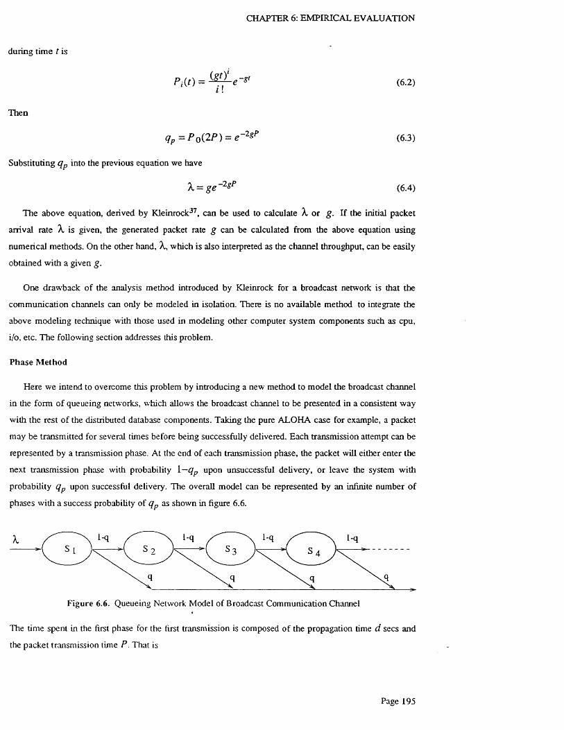
CHAPTER 6: EM PIRICAL EVALUATION
during time t is
(6.2)
Then
qp = P 0(.2P) = e - 1s l> (6.3)
Substituting qp into the previous equation we have
X = ge 2gP (6.4)
The above equation, derived by Kleinrock37, can be used to calculate X or g. If the initial packet
arrival rate X is given, the generated packet rate g can be calculated from the above equation using
numerical methods. On the other hand, X, which is also interpreted as the channel throughput, can be easily
obtained with a given g.
One drawback of the analysis method introduced by Kleinrock for a broadcast network is that the
communication channels can only be modeled in isolation. There is no available method to integrate the
above modeling technique with those used in modeling other computer system components such as cpu,
i/o, etc. The following section addresses this problem.
Phase M ethod
Here we intend to overcome this problem by introducing a new method to model the broadcast channel
in the form of queueing networks, which allows the broadcast channel to be presented in a consistent way
with the rest o f the distributed database components. Taking the pure ALOHA case for example, a packet
may be transmitted for several times before being successfully delivered. Each transmission attempt can be
represented by a transmission phase. At the end of each transmission phase, the packet will either enter the
next transmission phase with probability 1— qp upon unsuccessful delivery, or leave the system with
probability qp upon successful delivery. The overall model can be represented by an infinite number of
phases with a success probability of qp as shown in figure 6.6.
Figure 6.6. Queueing Network Model of Broadcast Communication Channel
The time spent in the first phase for the first transmission is composed of the propagation time d secs and
the packet transmission time P. That is
Page 195

CHAPTER 6: EMPIRICAL EVALUATION
S , = d+ P (6.5)
The time spent in the subsequent phases for the following retransmissions is composed of d , P and an
additional random wait W r which is used to avoid further collision. Thus
Si = d+ P+ W r
=s2*=2,3,' • •
Applying Cox’s phase method17, the Laplace transform of the above model is given by
/*<*)= z u V - ^ r i t f i Ti= I k= 1
1
s S i+ I
f V
Qp (1 Qp)1
S oS -------- h l _
Qp
(6.6)
(6.7)
The above Laplace transform / ( s ) implies that the queueing model has two phases. The first phase with
mean time S \ is compulsory. It clearly represents the first attempted transmission. After the first phase a
packet may be successfully transmitted with probability qp or may enter the second phase with probability
1—qp . The second phase represents the sum of the subsequent retransmissions. The total time used by
these retransmissions equals S 2!qp . The reconstructed model is shown in figure 6.7.
F igure 6.7. Reconstructed Queueing Model for Broadcast Network
The model can be interpreted as a network of queues with two infinite-server (IS) service centres, i.e.
the M I G / 0 0 queues. The mean number of customers, i.e. packets, in the system can be immediately
obtained by
and the mean transmission time
n = X S i + M l - q p ) — Qp
l ~ q pR = S l + ^ JLS 2
Qp
(6.8)
(6.9)
Substituting 5 1 and S 2 in the above equations, we have
Page 196

CHAPTER 6: EM PIRICAL EVALUATION
n = X
and
R =
d + P + - ^ - ( d + P + W r)Qp
d + P + ^ - ^ - i d + P + W , ) Qp
(6.10)
(6.11)
The results are extremely simple and easy to be applied to the queueing network model.
S lo tted A LO H A Protocol
The difference between slotted ALOHA and pure ALOHA is that slotted ALOHA divides transmission
time into slots which are equal to the transmission time of a packet, i.e. P sec. Each transmission is further
synchronized to the slotted time interval. Collisions only occur during one slot period. Therefore the
vulnerable period for slotted ALOHA is P sec rather than 2 / >sec. Upon collision a packet must wait a
random K slots before retransmission. Adopting the similar method used in analyzing pure ALOHA, we
can easily obtain the probability of no collision by
X
gQp
(6.12)
The phase method for broadcast network introduced above can be easily applied to the slotted
ALOHA. Thus the number of packets in the system is give by
n = X d + P + - ^ - ( d + P + W r)Qp
(6.13)
and the transmission delay is given by
R = d + P + — ^ -(d + P + W r) Qp
(6.14)
It should be noted that the propagation delay and the random wait of the slotted ALOHA are different
from that o f the pure ALOHA. They are measured by slots. Suppose the random wait of a packet is
uniformly distributed among 1 to K slots, that is, the packet will be retransmitted in one of the slots,
d + P ,d + 2 P , ■ * • , d + K P with equal probability. Therefore the average number of slots spent in the
random wait is
K - 1
Thus
Page 197

CHAPTER 6: EMPIRICAL EVALUATION
Wr =2
(6.15)
Substituting W r in equations (6.13) and (6.14)
we obtain
l - q „ K - 1R = d + P + — ^ ( d + P + ^ - ^ P )
<lP 2(6.16)
and
n — X
= g
1 - q p K - \d + P + — — ( d + P + ^ ^ P )
qP 2
K - 1
' CL
1
2(6.17)
It is interesting to notice the similarity between the results obtained by using the phase method
introduced by the author and that obtained by Kleinrock37. The- mean number of packets n obtained by
two methods are exactly the same. The mean packet delay R differs only in
qt = Prob [previously blocked packe t is successfully tran sm itted } (6.18)
given by Kleinrock and
qp = P rob {blocked packet is successfidly transm itted} (6.19)
given by the author.
The author’s method has an advantage over method introduced by Kleinrock37 in the sense that the
author’s method is consistent for all the broadcast type communication networks, and it is also consistent
with evaluation models used to estimate other components of computer systems such as cpu and i/o etc;
while the method introduced by Kleinrock can only evaluate some special algorithms, such as slotted
ALOHA and the evaluation can only be done in isolation.
E thernet
Now we can use the above method to evaluate the performance of Ethernet, shown in figure 6.8.
Ethernet is a bus network, which is used to connect a number of processing elements (usually computer,
terminal and i/o devices). The transmission medium o f the bus channel is usually coaxial cable. Any
number of processing element can be connected to the channel by a transceiver.
4The characteristics of the bus network are
• broadcast communication;
Page 198

CHAPTER 6: EMPIRICAL EVALUATION
• baseband transmission mode;
• small propagation delay.
Term inator
PE PE
T/CT/CT/C
T/C
T/C
T/CT/C
PE
PE
PE
PEPE
T/C = transceiver
PE = Processing Element
Figure 6.8. Bus Network
The nature of the bus network, especially the characteristics of short propagation delay, determines its
access strategy. The bus network employs a carrier sensing technique. The technique called carrier sense
multiple access (CSMA) is designed for local area bus networks. A sending user first listens to the channel.
If a carrier is sensed, the transmission has to be delayed according to some algorithm; otherwise the packet
is transmitted immediately. The transmission is vulnerable during a period at the beginning o f the
transmission. This period is equal to the one way propagation delay d l 2, which is much smaller than the
transmission delay. Therefore the vulnerable period of the bus network is very short compared with that of
ALOHA protocol. There are two types of transmission: slotted and unslotted. The slotted transmission is
achieved by synchronizing the channel into slots. A slot time is usually equal to one way propagation
delay.
The access control algorithm for the bus network can be classified into two mainly categories:
Deference/Acquisition (D/A) and the Collision Detection (CD) algorithms. Since Ethernet emploies the
later, we shall develop its evaluation method in details.
Collision Detection CSM A
Page 199

CHAPTER 6: EMPIRICAL EVALUATION
The collision detection CSMA, also known as Listen-W hile-Talk (LWT), is used to detect collisions
during transmission. As soon as a collision is detected, the transmission is terminated by transmitting a
jam m ing signal to ensure that all other users detect the interference and, therefore abort.
A typical LWT Ethernet is defined by IEEE 802.3 standard with the following parameters
data rate = 10Mbs
s lo t time = 5 1 2 bits
preamble = 64 bits
ja m signal = 32— 48bits
interframe spacing i.e. a = 9 .6— 10.6microsecs
A station, wishing to transmit, packs the data into a packet. It first listens to the Ether to sense a carrier.
Once the end of the carriers is sensed, it delays for a certain time to allow hardware to settle, i.e. interffame
spacing CX, and then transmits a preamble followed by the packet. The transmission is subject to collision
during a period of (X sec., where CX is also the one way propagation delay. Once the collision period is
passed, a station is said to have acquired the Ether and other stations are deferred for the duration o f the
transmission. One remarkable feature of Ethernet is its ability to detect collisions while transmitting.
Upon collision a station has to wait for a random period of time to retransmit the packet. The
retransmission is governed by a binary exponential backoff algorithm. For the /2th retransmission, the
transmission is delayed by r slots, where r is a uniformly distributed random integer in the range 0 < r < 2 k,
& = m in (/2, 10).
We shall first model the retransmission delay. In order to simplify the modeling, we assume k —n. This
assumption can be usually justified for non-heavily loaded network, since the retransmission times is
usually less than 10. Let us denote as the random delay of the £th retransmission. The probability of a
packet being delayed by r slots upon £th retransmission is given by
Pkir )={
_1_
2*l< r < 2 k
(6 .20)
0 othervw'se
The mean of P i f r ) can be obtained by
Page 200

CHAPTER 6: EMPIRICAL EVALUATION
Wk=XrP'Pkir)r = 0
* r P
r = i 2 k
1+ 2*(6.21)
where P is the transmission time.
LaBarre40 has derived a throughput equation for nonpersistent LWT CSM A protocol, which is written
as
x = g e- a g P 1
(6 .22)g P ( e ^ p '~+oP) + ( l+ o .g P 2) ( l - e ~ asF‘2 j1 + 1
where CC=d 12 is the one way propagation delay.
It should be noted that for a CSMA protocol, a deference time should be included. It is the time delay
between the start of the sensing and the moment at which a non-busy channel is sensed. Let us denote p ^
as the probability of sensed busy. Then g p ^ is the number of transmissions being blocked by sensed busy
and gpfyfX is the average number of times over which a packet is blocked. For each sensed busy, a packet
waits for a random period W r . The average deference time of a packet is therefore equal to gpi,IX
multiplied by one random delay W r. That is
gPbX
W r - average deference time o f a packe t (6.23)
It should be noted that due to the carrier sense nature of the CSMA protocol, the probability of a
successful transmission is no longer equal to XJg. Recalling the pure ALOHA protocol, g is both the
number of packets generated per sec and the number of packets attempted for transmission per sec. But inA
CSMA CD protocol the two are not equal. The number of packet attempted for transmission per sec g is
equal to the number of packets generated g multiplied by the probability (1 —pt>)- That is
g = g i \ ~ P b )
where /?£,, the probability of being blocked by sensed busy, is given by Tobagi82
(6.24)
1 + a g P
l + g / > ( l + a P + r )(6.25a)
and
Y = a P - — ( l - e ~ <xsp2)g P
(6.25b)
Page 2 0 1

CHAPTER 6: EMPIRICAL EV ALUATION
The probability of a successful transmission qp is therefore given by
qP = T = — r <6-26>g g ( i - P b )
Let us consider the average transmission time and the average number o f packets in the system. The
phase method proposed by the author can be used here. The time spent in phase one equals the sum o f the
successful transmission time and the deference time. That is
n u r n 3 _ gPbS I = P+OC+-T— W ! = P + a + - P - r - (6.27)
A 2 A
For the subsequent transmissions (z = 2 ,3 , ' * ' )• The transmission time 5 / is composed o f the
interference delay caused by the last conflicting transmission CX, the jamming signal delay P after the
transmission, the deference delay to avoid further conflict, the one way propagation delay a to clear the
channel, the packet transmission time P and the deference time. The retransmission delay is therefore
given by
8PhSi = 2 ( X + f > + P + ^ E- W i _ l
A
Substituting into the above equation, it becomes
S i = o + ^ - 2 i - 2P A
where
P gPbc = 2 a + p + / > +
2 X
It should be noted that the above retransmission delay Wt changes for each retransmission on Ethernet
due to the binary exponential backoff algorithm. We have to extend the phase method to model this more
robust retransmission algorithm. The model consists o f an infinite number of phases, where phase i has the
service time of S*. A transmission will terminate successfully with probability qp and continue to
retransmit with 1 —qp . The Laplace-Stieltjes transform of the model is given by
/ ( s ) = i ( i i , r ' ?, i i - L (os)i=1 y y k = isS k+ i
The mean is given by
Page 202

CHAPTER 6: EM PIRICAL EVALUATION
7 - / * ( * )o *=l *=1* = 1
/> gpfr
2^,-1 A.(6.29)
The results o f the above model suggest that the whole Ethernet can be modeled by an infinite-server (IS)
service centre with mean service time given by the above equation. The generating rate g can be obtained
from equation (6.22) and the probability o f being blocked by sensed busy p& is given by equation (6.25a)
and (6.25b).
The average transmission time is therefore given by
It is interesting to notice that the phase method introduced by the author is consistent in all the CSMA
results produced here are consistent with those available by using others’ ad hoc methods. The phase
method can be used conveniently in queueing networks to model broadcast communication networks.
As previously introduced, the DRFS is composed of two tiers, the TM -TM tier and the TM-DM tier.
The TM -DM tier manages the distributed executions of transactions between TM s and DMs. The
modeling o f the TM-DM tier for transaction management is of particular interest since it is the core part of
the system. The transaction management, as discussed in section 6.4, is controlled by a majority consensus
two phase commit protocol, i.e. P4. To model the concurrency control and locking performance o f the
TM -DM tier, it is necessary to employ the model derived for the general majority consensus 2PL protocol
on a packet switching network introduced in section 5.2. However, since DRFS is built on a bus network
(Ethernet) rather than a packet switching network, we shall combine the models o f Ethernet in section 6.7.1
and the majority consensus 2PL in section 5.2.
Suppose we model a DRFS system in which TMs and D M s do not share workstations. Its
communication structure of the DRFS is showp in figure 6.9. Applying the method introduced in section
5.2, the DRFS system can be modeled by an open queueing network with general service time
distributions. The equations used to solve the model are from (5.27) to (5.56). However the model requires
two modifications. Since T M and D M are not built on the same workstation, a transaction generated at
(6.30)
and the average number of packets in the system
(6.31)
protocols studied. It models the bus network in a natural way and has clear physical explanations. The
6 .6 .2 A n a ly tic M od el o f the O vera ll System
Page 203

CHAPTER 6: EMPIRICAL EVALUATION
User TM
DMDB
DMDB
User TM
User TM
DMDB
Figure 6.9. The Communication Structure of the DRFS
Page 204

CHAPTER 6: EMPIRICAL EVALUATION
T M will only access remote DM s. The access pattern matrix is modified by
1— i e T M , i s D M Nf
0 otherwise (6.32)
In a packet switch network, the communication channel between station i and k is modeled as a single
server service centre; while for a bus network, the whole bus can be modeled as one infinite-server (IS)
service center as introduced in section 6.6.1. Since an IS service centre can be decomposed into many IS
service centers, for the sake of simplicity we can use an independent IS service centre for each i to k
communication, denoted by /*. According to equation (4.111), the mean number of busy servers of the i to
k service centre is given by
2Kcik + — +1 (6.33)
where
Cik = T - I l K C r l ) p jit + l ] k j P j ik j =o
(6.34)
is the squared coefficient o f the variation of the interarrival time at service centre i£. The mean service
time of the Ethernet IS service centre is given by equation (6.29). That is
SPb1-<h , f u, = a h —a h-------<lP 2cIP~ l
(6.35a)
Where Pb is given by equations (6.25a) and (6.25b). In the DRFS implementation, the majority consensus
2PL protocol is built on the top of the transport layer protocol UDP/IP. In order to save cpu time of the
listening server, the protocol uses a small time-out delay to select incoming messages. Therefore a further
delay factor W p should be added to the service time |Xl t . That is
\--qP , pJl; = CM- <X+Qp
- ^ + W P2qp- [ X(6.35b)
Since all IS service centers share one Ethernet, the overall throughput of the Ethernet is the sum of all the
interarrival rates to the network. However the cost o f multicasting a message to N acc receivers is the same
as unicasting the message. Therefore at each phase of the majority consensus 2PL Ethernet only transmit
14-Nacc rather than N acc+ N acc messages. The overall throughput of the Ethernet is therefore given by
x =[+Nacc « *
2N* X I L K (6.36)acc ; = U = l
Substituting X into equation (6.22) we can obtain the generating rate g from

CHAPTER 6: EM PIRICAL EVALUATION
1 +Nacc K K ee-°*p2a c c y y _ ___________________________ <5£___________________________________ 3 7 }
INacc / = u = i '* g P ( l + 2 a P + 2 a P e ~ agl‘*) - ( \ - e ~ asp1)1 + 1
The probability of blocking by sensed busy is given by equation (6.25a) and (6.25b) respectively. The
model can be solved iteratively by numerical method.
Previous researches can only evaluate distributed database built on point-to-point network. We have not
only introduced a novel metod to evaluate bus netowrk (i.e. Ethernet) but also integrate it naturally with the
overall queueing netowrk model; thus our anaylytic model covers all the types o f networks.
6.7 Performance Measurements and Comparison of Results
The DRFS system is tested by using performance measurement method. The analytic model o f the real
system is also built and analytic results are obtained. T he comparisons of the measurement and analytic
results are shown in figure 6.10 and 6.11.
Throughput
. 5 - ---------------- Analytico o o o o Measurement
. 4 -
.3 -
0 1 2 3 4 5Think Time (in seconds)
F igure 6.10. Throughput of the DRFS System
Page 206

CHAPTER 6: EMPIRICAL EVALUATION
---------------- Analytico o o o o Measurement
U seful
cpu 0 0 8
0.06
0 3 41 5Think Time (in seconds)
Figure 6.11. Cpu Utilization at a D M in the DRFS System
The DRFS being measured v is composed of two TMs and three D M s as shown in figure 6.9. The
aim o f the measurements is to obtain the mean throughputs and system utilization of the DRFS. The files
stored in three DMs contains 100 records, and each record owns a lock. At each TM, a large number of
transactions are generated by a test program. Between two successive transactions a wait is imposed to
simulate the think time. By varying the think time from 0 sec to 5 secs, a group of mean measurement
results are obtained. The throughput of the DRFS is measured by counting the number of the transactions
completed during the test period. The useful cpu time is obtained by running the "time" command to
generate a profile o f the DM server process.
In order to obtain the analytic results o f the tested DRFS, several measurement tests have been run to
obtain the mean and variance o f the service times of locking, reading and writting records, and protocol
delay. These measured parameters are then used in the analytic model of the DRFS. The results are
illustrated in figure 6.10 and 6.11 along with the measurement results.
The analytic model of the DRFS represents very detailed characteristics of the system, such as the
concurrency control algorithm, database structure, Ethernet protocol algorithm, data granularity, degree of
data replication, service time distributions of the cpu and i/o devices, etc. It aims to give an accurate
evaluation of the real system and provide validation for the analytic model. These two goals are achieved
as indicated by the close agreement between the results. Furthermore, from this validation we have
presented the real physical interpretations of the analytic model and gained many useful experiences on
Page 207

CHAPTER 6: EMPIRICAL EVALUATION
how to apply performance evaluation theory into real systems.
The comparison of the two results indicates a satisfactory agreement between the analytic model and
the real system. Therefore the analytic model is validated by not only the simulation results but also more
convincingly an actual distributed database. This kind o f emparical valoidation has not been done before,
because it is not a simple task to implement an actual distributed database and it is also difficult to include
detailed characteristics o f the system in the analytic model. We have not only managed these two difficult
tasks, but also achieved a high degree of accuracy in emparical validation.
6.8 Summary
In this chapter, an actual distributed database management system is implemented. The system uses
basic 2PL and majority consensus 2PL algorithms and it furhter employs many novel features such as
multicast communication premitives, dynamic TM configuration, failure recovery etc. Novel analytic
model has been introduced to evaluate bus-network and its integration with the overall model o f the
distributed database. Results from empirical evaluation agrees with the anlytic results at a high degree of
accuracy; thus adding further validation support to the theory.
Page 208

Chapter 7. Conclusions
7.1 Conclusions
In this thesis, consistent and systematic methods have been used to study the performance of
concurrency control protocols in both centralized and distributed databases by using analytic modeling,
simulation and measurement. The models have captured many important features, such as transaction
blocking, priority locking, multiple transaction classes, concurrency control algorithms, collision resolution
algorithms, service time distributions, locking granularity, data replication, network topology and network
protocols.
Original contributions have been made in the thesis to develop and extend the modeling techniques
throughout all the levels. We can define the basic level as a fundamental representation of the architecture
and concurrency control algorithms in a distributed database system; the first order level as the factors
which have a first order effect to the performance of a distributed systems, such as the mean measurements
and queueing disciplines; the second order level as the additional factors which only have a second order
effect on the performance, such as the variations and distribution functions.
A t the basic level the introduction o f the communication flow rate matrix, access pattern matrix, and
Markov chain matrix has brought a valuable step toward the representation o f the fundamental architecture
o f the concurrency control algorithms and the underlying network topology of a distributed database in a
consistent and systematic manner.
At the first order level, novel methods have been introduced to model waiting in blocked queue, priority
queueing and multiclass transactions. Many important factors such as the degree of data replication,
degree of the locality, read-write ratio and locking granularity are modeled to achieve a high degree of
accuracy.
At the second order level evaluation methods have been introduced in the thesis to model distributed
databases with non-Poisson interarrival distributions and general service time distributions. The second
order factor, i.e. the variation of a random variable in the queueing network is represented by applying
extended diffusion approximation method. Moreover the service time distributions of various database
operations and data transmissions are given by statistical analysis and measurements.
The analytic models proposed in this thesis are validated by simulation results obtained by both the
author and Ries and Stonebraker. The comparison of results shows a very close agreement between the
two. The comparison of results obtained from the analytic model and from the actual distributed database
system implemented by the author also indicate a close agreement between the two. The research
introduced in the thesis provides a significant step forward in performance eveluation of distributed
Page 209

CHAPTER 7: CONCLUSIONS
databases. The main contributions made in the thesis are as follows.
One of the most difficult problems associated with database modeling is to evaluate the waiting time of
blocked transactions. In this thesis we have introduced a novel method to solve the problem. An analytic
model is used to represent a centralized database as a network of queues. In particular, the blocked
transactions in the waiting queue are modeled by an infinite number of infinite-server service centres, each
o f which represents a waiting phase of the blocked transactions. The stochastic nature of blocking and
collision resolution algorithms is therefore accurately modeled. The overall model of the centralized
database with blocking is represented by an open system composed of A //G /1 and IS queues with two
priority levels. The technical methods used to solve the analytic model are developed in the thesis. Firstly,
since locking operation has priority over transaction execution operation, the method to model two priority
levels has been introduced. Secondly, the distribution function of the departure process of the transaction
execution jobs, i.e. second priority class jobs, is derived to model the waiting phase of the blocked
transactions. Thirdly, the transactions with non-exponential service time distributions are modeled by
including the second moment of the service time distribution in the model.
The open model of the centralized database is further extended to the closed model by introducing an
approximation method, from which a very useful approximation result has been obtained: under the
condition of small lock overhead, the departure process of the transaction execution job is approximately
Poisson and its mean depends only on the overall throughput of the closed database.
Further numerical technique has been introduced to model the multiclass transactions in the blocked
queue. The service demands, lock conflict rates and lock sizes of different classes of transactions are
represented. An interesting phenomenon, that the transactions with smaller service time and lock size will
circulate in the system more quickly than others, has been noticed.
In order to validate our analytic model o f centralized database, we have used Ries and Stonebraker’s
simulation model and results. Their model simulates the centralized database at a very detailed level, such
as transaction blocking phenomenon, collision resolution algorithms, locking and transaction operations,
lock script and multiclass transactions. By comparing our analytic results with their simulation results, we
obtain a close agreement between them.
A novel method is introduced to systematically define a distributed database system with two phase
commit concurrency control protocol. A distributed database is composed o f network service centres,
computer service centres and locking service centres. The data flow between these service centres depends
on the concurrency control protocol, data replication, lock granularity, read-write ratio, network topology
etc. In this thesis, we first introduce the concept of access pattern matrix and communication flow matrix,
which represents the flow of data between service centres. The arrival rate matrix is further derived to
define the interarrival rates of transactions to each service centre and finally the Markov chain matrix can
be derived from the communication flow matrix to define the overall queueing network. The method very

CHAPTER 7: CONCLUSIONS
m uch simplified the complicated and tedious task of manually obtaining the Markov chain matrix of a
distributed database. And it is also proven to be very useful in developing the distributed locking model in
section 4.3.1.
Transaction blocking in distributed databases has not been analytically modeled before. In this thesis
we have first introduced a phase method to model distributed locking with fixed waiting. The model can
represent each lock operation, the stages o f locking and the stochastic nature of locking. The method can be
easily applied to model various different types o f locking algorithms.
Previous researches only model distributed databases with exponential service time distributions. In
order to model general service time distribution and non-Poisson interarrival time, we have adopted and
further extended the diffusion approximation method. In the thesis new equations have been derived to
model infinite-server service centres. Furthermore the extended diffusion approximation m ethod is also
used to model distributed locking. The overall distributed database model is constructed by an open
queueing network with general service time distributions. The method can be extended to model various
distributed database systems and the numerical solution can be obtained with good convergence.
The overall distributed database model has captured most of the features of the system in a depth which
has not been reached before. It includes the communication flow of the concurrency control protocol,
locking algorithm, collision resolution algorithm, data replication, lock granularity, read-write ratio,
priority locking, service time distribution and interarrival time distribution. The model therefore can
represent the real system much more accurately.
The model for distributed database is also consistent and easy to apply to various concurrency control
protocols. The same model is used to model four different 2PL protocols. They are basic 2PL, primary
copy 2PL, majority consensus 2PL and centralized 2PL. The formal definition method, i.e. the access
pattern matrix, communication flow matrix, etc., is proven to be particularly useful in defining these
models. It makes the model definition task much easier and efficient. Furthermore since the same modeling
method is applied to these distributed database systems, the comparison of results are fairer. The method
can, in general, be easily applied to various other distributed systems with different concurrency control
protocols.
A simulation model has been built to validate the analytic model o f distributed databases. The
simulation model represents most of the characteristics o f a distributed database. It also simulates various
service time distributions to validate the extended diffusion approximation approach. The comparison o f
analytic results and simulation results clearly shows that the extended diffusion approximation model can
represent the system much more accurately than conventional queueing network method. The overall
analytic model achieves a high degree of accuracy in comparison with the simulation model.
In order to further validate the analytic method and show the real application o f the modeling, we have
implemented an actual distributed database system. The prototype system is built on several Sun
Page 211

CHAPTER 7: CONCLUSIONS
workstations over Ethernet, a bus network. One o f the main features o f the system is multicast
communication. Other features include basic 2PL and majority consensus 2PL protocols, dynamic TM
configuration and failure recovery. The prototype system is tested and measured.
In order to model the actual distributed database with multicast communication, an analytic model is
introduced to evaluate Ethernet. The method can not only evaluate isolated Ethernet but also integrate it
with the rest of the modeling method introduced in the thesis. Thus an overall analytic model for the
prototype distributed database with multicast is built. It represents detailed characteristics of the system,
such as concurrency control protocol, database structure, multicast protocol, Ethernet structure, data
granularity, data replication, service time distribution, etc.
The comparison of the analytic results and the real system measurement results shows a close
agreement. The analytic method is therefore further validated by real system measurement. M oreover the
validation also presents the real physical meaning o f the analytic model.
The comparison of various concurrency control protocols shows that, in general, centralized 2PL
outperforms basic, primary copy and majority consensus 2PL. It is interesting to notice that the locking
conflict rate is strongly associated with the distribution o f the locking activities. The wider the locking
activities are spread, the higher the conflict rates are. Another interesting finding is that the degree of data
replication has a big impact on the response time. By properly choosing the parameter, optimal
performance can be obtained. The finding of lock granularity being less effective to the overall
performance is not surprising, since the lock overhead in the test system is quite small. These performance
results are useful in comparing various concurrency control algorithms and designing distributed database
systems.
In conclusion, many original methods have been introduced in the thesis to model concurrency control
and locking in both centralized and distributed databases in greater depth than before. All the analytic
methods introduced in the thesis are validated by either author’s simulation model, others’ simulation
model or real system measurement. Various concurrency control protocols have been modeled and
analyzed and many interesting results have been obtained in the thesis.
7.2 Future Directions
Research could be carried further in the following directions. Firstly, in order to further improve the
accuracy of performance evaluation, there is a requirement to represent the functionality of the
concurrency control in more details, such as that achieved by simulation. Secondly the assumption of no
site or network failure can be released by introducing the probability of failures in the model. Thirdly the
effect of work load is not modeled in the thesis. However it is not difficult to include it in the queueing
network model in a consistent way. Fourthly the modeling of both exclusive and shared lock in a
distributed system requires further attention. New probability descriptives such as the percentage of shared
lock and exclusive lock can be introduced in the analytic model.
Page 212

Appendix A. List of Notions
(X one way propagation delay
P jamming signal delay
Laplace-Stieltjes transform o f the service time distribution o f the zth priority level
Jik mean message rate for those originated at node z and terminated at node k
y rWk read-write ratio o f a transaction generated at T M ^
5 inter-track movement time
0 ^ residual interanival time o f the second priority customer
X mean interanival rate
Xq mean interarrival rate at the source
X}, mean interarrival rate of a blocking service centre
X^pu mean interarrival rate of the zth priority customer at a cpu service centre
X\lJ mean interanival rate of the zth priority customer at an i/o service centre
X\j* mean interanival rate of communication channel from node z to node j
mean interanival rate of node k at stage S
X ^ mean interanival rate of the zth priority customers
Ac communication flow rate matrix
A | throughput of service centre z
A s arrival rate matrix at stage S
JJ, mean service rate of a job
(l(z?) aggregated service rate of the inner model of a computer system at the
mud programming level o f n
mean interdeparture time o f a transaction execution centre
Page 214

APPENDIX A: LIST OF NOTIONS
|1 0 mean residual interdeparture time of a transaction execution centre
mean interarrival rate
|l ag aggregated service rate of a locking service centre with fixed waiting
\lfj mean service rate of a blocked queue with fixed waiting
|liock mean service rate o f lock request
(X . mean service rate o f a class i transaction in service centre k
Jlj mean service rate of requesting one lock
mean service rate of the zth priority customer
1) Laplace-Stieltjes transform of the busy period of the zth priority level
initial waiting time of residual busy period of the first class customer
number of zth priority customers in the system prior to the arrival of the /zth
customer
IT, stationary distribution of z customers in the system
Ft,* path between node i and k
p utilization
C5 second moment o f the service time
<5a standard deviation of interanival time
standard deviation o f service time
<3a variance of interarrival time
7<JS variance o f service time
second moment o f the Zth priority customer
O* ( s ) Laplace-Stieltjes transform of the service time distribution of one locking
operation
Xn epoch of the /zth arrivirlg customer
ti)/y probability of a transaction accessing node j from node /
Page 215

APPENDIX A: LIST OF NOTIONS
a overall system utilization
a utilization at the zth priority level
o f f communication flow rate from node i to j at stage S
A ( t ) cumulative number of arrivals up to time t
A , communication flow matrix between stage Z and Z + 1
b ( t ) service time density function
busy period o f the first priority customer
B (f ) service time distribution function
B l k length of a block
c number of transaction classes
ca coefficient of interarrival time
Ci capacity of the zth communication channel
C; completion time of a second priority customer
Cs coefficient o f service time
C i squared coefficient of the variation o f the interarrival time at service centre z*
Ct y uj service capacity of the class j customer at the zth priority level at the cpu service
centre
C \ lJj service capacity of the class j customer at the zth priority level at the i/o service
centre
d propagation time o f a packet transmission
D (t) cumulative number of departures up to time t
D ^pUj service demand of the class j customer at the zth priority level at the cpu service
centre
D^iqj service demand of the class j customer at the zth priority level at the i/o service
centre
dm —read (X ) Read (X ) performed on a physical database by a D M
Page 216

APPENDIX A: LIST OF NOTIONS
dm —write (X ) Write (X) performed on a physical database by a D M
DMfi. data manager at node k
et relative throughput of service centre i
f lo c k (s ) Laplace-Stieltjes transform o f the service time distribution of locking operations
to grant r locks
*f Laplace transform of function /
fb ( s ) Laplance-Stieltjes transform of the service time distribution of the waiting centre
/ (x , t ) probability of X jobs at time t
File length of a file
g packet generation rate (i.e. number of packets generated per second )
g attempted packet transmission rate
* f \g r \ S ) residual life time of the density function of the interdeparture process of the
second priority customer
]|Cg (5 ) Laplace-Stieltjes transform o f the density function of the interdeparture process of
the second priority customer
G normalizing factor of an open queueing network
G{r i) normalizing constant when the number of customers in the system is n
G { t ) distribution function of interanival time
G { t ) approximate service time distribution of the interdeparture distribution of the
second priority customer
jjt
G ( 5 ) Laplace transform of G (t )
G ap length o f a gap between blocks
service time distribution function of the i priority customer
K number of nodes in a distributed database
Ki squared coefficient of the variation of the service time
/ number of levels o f an index
Page 217

APPENDIX A: LIST OF NOTIONS
l l message length of the ith communication channel
l l vector of a 1 in the ith component and zeros in the rest
L total number o f locks in the database
L k total number o f locks in the database at node k
lock (X ) apply lock on data item X
m number of service centres
n a average number o f accesses for each record
n.[ number of customers at service centre i
rip mean number of paging activities of a customer
n r number of records in a file
n r number of indexable records
Tii mean queueing length of service centre i
n k. mean queueing length of the ith communication channel at node k
n \ . mean queueing length of the ith communication channel at node k at stage S
n k mean queueing length of class i transaction in service centre k
n * mean queueing length of the ith priority customer
N number of customers in the system
N acCk mean number o f database accesses to D M generated by one transaction at a T M
N f mean number o f replicated data copies
total number of granules in the database
Nn mean number o f locks held by class i transactions
N mean number o f busy servers in an infinite-server service centre
N vector of the total number o f transactions in each class
N L ^ o m l ) mean number o f locks held at the communication channel in stage 2 at node k
Page 218

APPENDIX A: LIST OF NOTIONS
N L [ com3) mean number o f locks held at the communication channel in stage 3 at node k
N L ^ mean number o f locks held at the lock request centre at node k
p ( n ) diffusion approximation to the probability that the queueing length is n
Pb probability of sensed busy
Pjb probability of feedback
P ij probability of a customer moving from centre i to j
P packet transmission period
P ( n ) probability o f the state of n customers
PinQ,ni, . . . , r i /c) steady-stage probability of a network state with k + 1 service centres
P i( n i ) factor corresponding to the steady-state probability o f the state o f service centre i
in isolation
P i iO probability of i transmissions during time t
P rob {A ccesS jje} probability of accessing node k from node i
Prob {R e a d } probability of a transaction being of read type
Prob {Write } probability of a transaction being of write type
q probability of successfully granted one lock
qb probability o f successfully granted r locks
q k probability of successfully granted one lock at D M k
qp probability of successful transmission of a packet
q t probability of previously blocked packet being successfully transmitted
Q ( 0 number of customers at time t
r average number of locks held by one transaction
r mean number o f locks required by one transaction in all transaction classes
rl rotational lantency
rpm number of disk revolution per minute
Page 219

APPENDIX A: LIST OF NOTIONS
R*, mean response time o f class I transaction in service centre k
Ri mean response time of service centre i
R eadiX ) transaction o f reading logical data item X into database
Rec length o f a record
sc initial startup time of an i/o device
Si time spent in the ith phase o f transmission
Sn service time of the nth customer
sk seek time o f a disk
*B block transfer time
record fetch time
(R record transfer time
t' bulk transfer rate
T raw transfer ratio of an i/o device (in chapter 2)
Ta average turn-around time of a closed queueing network
TMk transaction manager at node k
U % j utilization of the class j customer at the ith priority level at the cpu service centre
Vi utilization of service centre I
u t t j utilization of the class j customer at the Ith priority level at the i/o service centre
utilization of class / transaction in service centre k
W; pre-waiting time of the second class customer
w access pattern matrix
Wa waste of a disk
wk random delay of the kth retransmission
wV¥p time out delay at transport layer
Wr random waiting to avoid further collision
Page 220
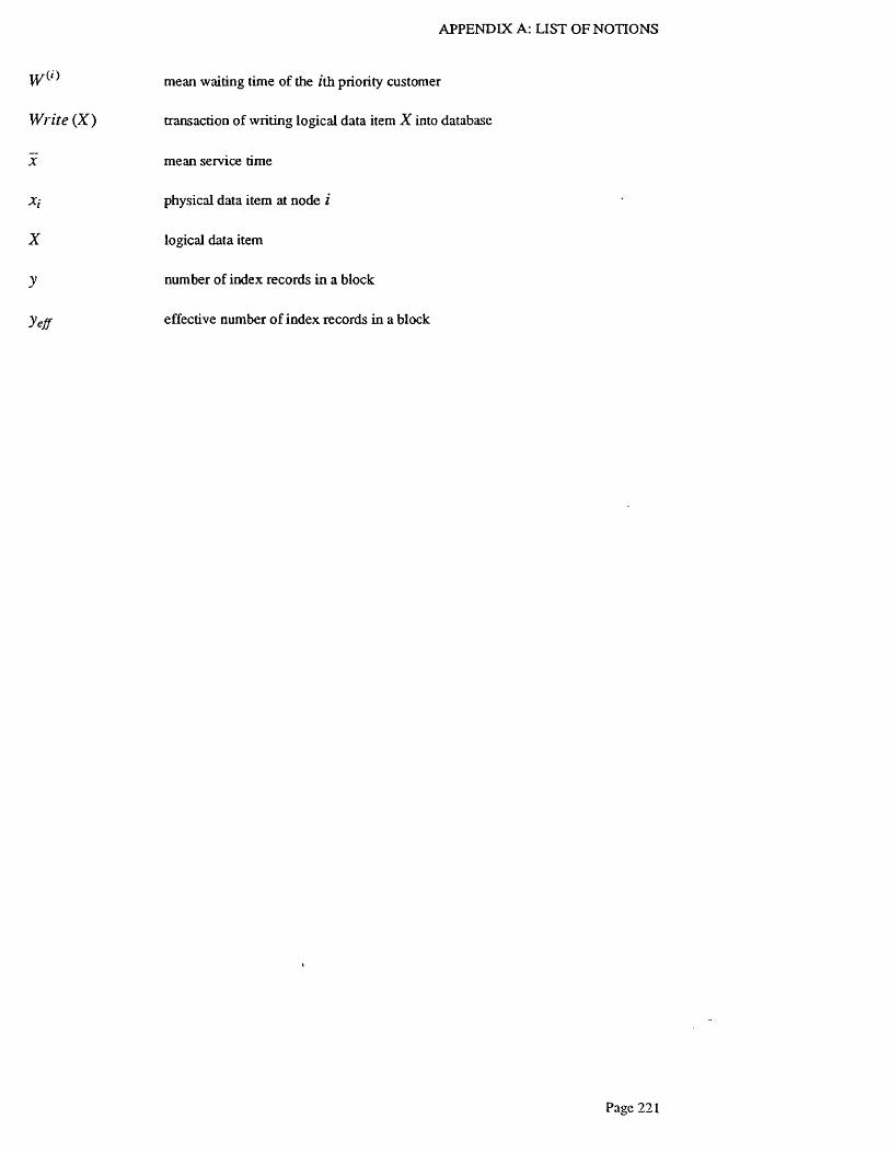
APPENDIX A: LIST OF NOTIONS
jyO') mean waiting time of the i th priority customer
W r i t e ( X ) transaction of writing logical data item X into database
X mean service time
physical data item at node i
X logical data item
y number of index records in a block
yeff effective number o f index records in a block
Page 221

Appendix B. Theorem Proof
The theorem proofs of chapter 3 are included.
T heorem 3.1: The process [0 ,°°)} which is regenerative with respects to the renewal precess
V , , / e [0 ,° ° ) is Markovian with a standard transition matrix 7l i j ( t ) , i J ^ S such that for all i , j&S,
( 0 P i j ( t ) = ' Z r ikn k j( t ), f> 0 ,keS
( i i ) fo r /t= 0 , > w > 0 ,
Pr{x%)=jh'U<th v,h=l,...,m\Sn+1=v,Sn=u,x9J=i}
~ P i j l W 1 7*2 (^2 ' l ) ’ * *
for j h . . . , j m ,i< E S ,w ith u < t1< t2 < • * * < fm<v, a n d m = 2 ,3 , . . .
(B .la )
(B .lb )
Proof: W ithin the time of two successive departures of the second priority customers there is no decrease of
while the increase of follows a Poisson process with mean Therefore there exists a
standard transition matrix 7Cfy(/), i J ^ S , such that for all i , j s S
^ Piy’( 0k&S
where
^ { X / 2)= y iX («2)= L 5 n= « ,5 n+1= v} , 0 < w < f< v(B.2)
t< u
without losting generality, we assume that U = 0 , therefore
, 0 < /< v
0 , t < 0
It should be noted that between two successive departures of the second priority customers
S n= u < t< v = S n+ i the number of arriving second priority customers forms a Poisson process. Therefore
during t — u time interval
Page 222

APPENDIX B: THEOREM PRO O F
It can be rewritten as
p ( t - u ) =
J (j- 0 !
/ x o s 2)t y 1 _\(2)rP ij{0 = , . _ / m e K (B.4)
<J - i )
This is obviously a pure birth process with transition m atrix given by
(.x {2)t y ~ i _x<2>,K i j ( t ) = — — — e A (B.5)
0 - 0 !
and
f 1 » i0 = *r i} = lim pf.-(f)=s (B.6)
|0 , if 'j± i
Hence
7. Vit A/CO — P U j (/ )AeS
=
= P i j(0
which satisfies the first condition of a regenerative process being a Markovian.
From the definition of P i j ( t ) we can immediately obtain the right hand side o f the second condition.
, , , , , , [ ^ ( f n o f ' - 0Pij, ■ ■ ■ K j ^ j J t n - t ^ O = -------- — ---------- e--------------- U l - J l ) ' - --------
(Jm jm — 1 )!
e
In order to obtain the left hand side o f the second condition, we use the M arkov property o f the inter-arrival
process
Page 223

APPENDIX B: THEOREM PROOF
\S n+l= v,Sn= u ,x?J= i}
)=jm,tni-i<t»i^v\%(j?)= j lt,u< th<tm, h = l , . . . , m - l , S n+i=v ,Sn=utx ^ = i } -II -t v (2)Xrm
Pr v (2).
K.
CLII v (2)X/m
Pr v (2):X/*
K.II v (2)Xrm
Pr /y (2)Xtm_
jm > — 1 I %(m_\ jm —1 }
,(2 ) _
Pr l x i 2 ) = y i , « < ' 1 ^ 2 1 5 n + i = v , 5 „ = M , x g >= z }
= [X(2)(;i-* O J0 l ~0 [Xc2)( r2—r 1)3C/2~Jl> - x « 0 W l)
O’1 -0 ? e O W i ) !
C/m 7 m —1) •[X(2>(fm- » ) ] (y"~ ,) -------------------------- £7 '
0 m - 0 !
Hence the second condition o f the theorem is also satisfied [].
T heo rem 3.2: The Laplace-Stieltjes transform of the completion time C; o f a second priority customer
with preemptive resume priority discipline is given by
E {e ~ sc‘ ) = £ j e ~ s' e~xm'dH{2)(t ) l \ la \ s , 1))*k =00
= P(2)U+X(1)( l-H (1)Cs, 1))} , Re5>0 , (B.7)
with
P(2)(^ )= \ e ~ srd H {2\ t ) (B.8)
and JLL^(.y, 1) defined as the Laplace-Stieltjes transform of the busy period o f the first priority level.
|X ^ ( s , 1) is the zero with the smallest absolute value of
(B.9)
with
(B.10)
Page 224

APPENDIX B: THEOREM PROOF
Proof: The probability of k interruptions from the first priority customers during a service time t of a
second priority customer is given by
k \
Let B ^ \ t ) be the distribution function o f the busy period of first priority customer. The total completion
time of a second priority customer with k interruptions can be easily written as
where is the &-fold convolution of the busy period with itself. The Laplace-Stieltjes
transform of the above equation is given by
oo oo
(2)( f ) * 0 B a > ( r ) ) ‘ * = 1 ))* (B .U )0 0
Since the interruption time and service time are independent to each other it follows that for the completion
time o f second priority customer we have
E { e sc' ) = £ \ e ~ st (X(Uf e - xW,d H a \ t ) { ^ l ) {s, 1)}**=00 * •
0 *=0 k '
0oo
0
= P ( 2 ) { j + X ( 1 ) ( l - l i ( 1 ) ( 1y> 1 ) ) }
T heorem 3.3: The Laplace-Stieltjes transform of the pre-waiting time w n o f a second priority customer is
given by
r t . ~sw- i - i H i (1)Q .(2), t ) ]s+X{1) [ \ a , +A.(2)-X (1)|xU)(X(2), l ) ] ( l - s /X i2))
Proof: We note that the moments at which a second priority customer leaves system is the regeneration
points o f the process, because at such moments no first priority customer are present at the system. If
the /tth second priority customer leaves the system empty, the pre-waiting time of the ( /2 + l) th customer,
i.e. the time between this moment and the moment at which the server becomes available to the (/2 + l) th
arriving second priority customer is the sum of the inter-arrival time of the (/2 + l ) th second priority
customer, denoted by 0^+1. anti the duration of a residual busy period o f the - system. This residual
Page 225
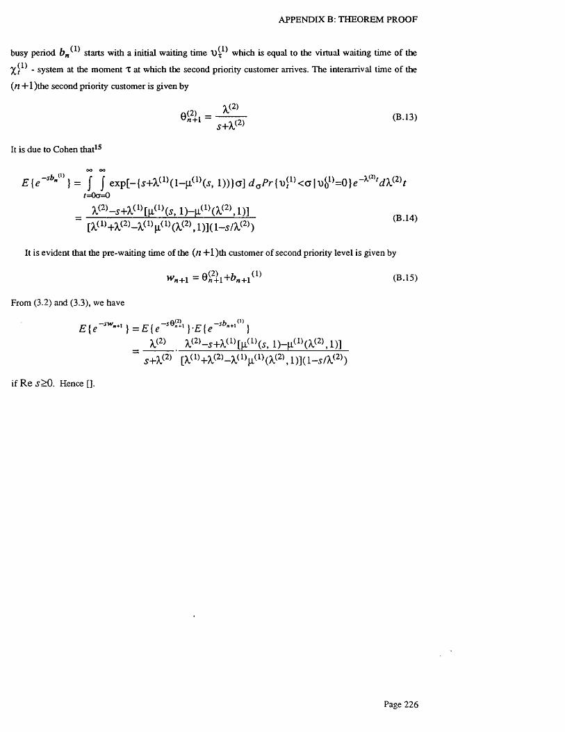
APPENDIX B: THEOREM PROOF
busy period b n ^ starts with a initial waiting time which is equal to the virtual waiting time of the
- system at the moment T at which the second priority customer arrives. The interarrival time of the
(n + l)th e second priority customer is given by
n(2) X 2)< > ■ '»
It is due to Cohen that15
OO OO(1)
E { e sb~ } = J J exp[-{i+X(1)(l-p.(1|(i, l)) |a ]/ = 0 ( 7 = 0
= X(2)-s+Xa )[n(1)c?, 1) - h(1)(A.(2>, D1 [5l< 1) +XW-X<-» » (X<2>. 1 )](l - i /x < 2>)
It is evident that the pre-waiting time of the (n +1 )th customer of second priority level is given by
^ + 1 = e < 2l i + f r „ +i (1> (B .i5 )
From (3.2) and (3.3), we have
E { e ~ sw"" ) = £ { e _se"' )-£{<rli"*1'" )X<2> X(2>- 5 + X ( l ) [n ( l ) (^, 1 )—n a >(X.<2> , l ) ]
s+X(2) [X(1)+X<2)-X.a V (1)(X(2), l) ] ( l-s A.(2))
if R e £ > 0 . Hence [].
Page 226

Appendix C. Evaluation of Service Time Distributions
Introduction
In recent years, considerable amount of research work has been done in analytic performance
evaluation of databases and computer networks6,27,37,66,77,81 However in most analytical models,
exponential service time distributions are assumed without actually verifying it with the real system. But
the usefulness of the analytic model depends very much on the specifications of the service time
distribution of each component in the system70. Unfortunately very little study has been done in this area.
The reasons are due to the difficulty and expensiveness of collecting the necessary data for the evaluation,
lack of good methods to estimate the theoretical distribution accurately from the observed data, and the
complexity of using general service time distributions in analytic model.
Although Coffman and Wood have pointed out that the distribution of interarrival time is a biphase or
triphase hyperexponential distribution14, and Fuchs and Jackson have suggested that the user think time has
a lognormal or gamma distribution23, very little study has been done in the estimation of the service time
distribution. By ignoring the actual service time distribution and assuming an exponential distribution, the
analysis o f computer system could be made easier, but its accuracy suffers. In order to evaluate the existing
computer systems accurately or provide a valuable guide to computer system design, the specification of
the service time distribution is necessary23,70.
In this section, we introduce an efficient method to evaluate the theoretical distribution functions of the
service time of some computer system components and to decompose the distributions into several stages
which can be easily applied in analytic models. Our method consists o f three major steps. Firstly
experimental models have to be built to collect the statistical data. i.e. the service time of the system
components. For instance the inter-computer communication service times, and the database processing
time are recorded which form the samples of the service time probability distribution function. Secondly a
method is introduced to evaluate the actual distribution function based on the collected data, and the results
o f % tests of goodness of fit is presented for each fit to prove the hypothetic distribution to be acceptable.
The probability distribution functions obtained from our model suggest that the distributions are of
hyperexponential nature with starting point not necessaryly at zero. Thirdly Laplace transformation is
performed to decompose the distribution into a form which can be presented with several stages. This
allows an easy application in analytical evaluations54.
E xperim ental Models of Service Tim e D istribution M easurem ents
The experimental models we have built are designated to evaluate the performance of two different
types of components, the inter-computer communication and database processing. The model for inter-

APPENDIX C: SERVICE TIM E DISTRIBUTIONS
computer communication is built on a local area network Ethernet. The communication is based on the
4.3BSD Interprocess Communication (IPC) facilities for UNIX43. The basic building block for this
communication is the socket Sockets exist within communication domains which are an abstraction
introduced to bound common properties of processes. All our experimental workstations run the 4.3BSD
Unix operating system. The experiment is carried out by using User Datagram Protocol (UDP).
The experimental model consists o f two processes as shown in figure C .l. One is the coordinate
process, the other is the participant process. The coordinate process generates UDP packets, while the
participant process receives and sends them back to the coordinator. The coordinate process therefore
gathers the statistical information of the round trip delay o f the interprocess com m unicatioa One way
communication delay can be easily obtained.
forward forward
backward backwardstation 1
Work-
CP
Ethernet station 2
Work-
PP
Figure C .l . Interprocess Communication Model
Two types of communications have been tested. One is called connection-oriented communication. A
connection is set up before communication starts; then each interprocess communication only involves
sending and receiving sockets. The other one is called connectionless communication which can be
typically found in the datagram facilities in contemporary packet switched networks. For each
communication a datagram socket is created with a name bound to it. Each communication delay of the
connection-oriented communication is comparatively sm aller than that of the connectionless if the time
spent in setting up the connection is excluded. This connection set-up time can be omitted if the number of
communications of each connection is very big.
In order to get the service time of the communication excluding the queueing delay and background
load, the experiments were carried out in the evening when the Ethernet traffic is negligible. Data were
collected on a weekly basis in the midnights. The packet size is 1024 bytes. Packets were sent in sequence
to avoid queueing.
In order to test the generality of our method, another experiment model is also used to evaluate the
database processing time. The experiment is based on the relational database UNIFY on Pyramid-9020
mainframe. Three types of database queries are being tested. Type I is a simple and frequently used read-
from-a-relation type o f query. Type II is a more complicated join type query. Type IH is a collection of
various different types of queues. All the data are collected in terms of service time of database processing.
Page 228

APPENDIX C: SERVICE TIM E DISTRIBUTIONS
Estimation of Probability Density Function
Here we introduce a method to approximately represent the observed discrete service time distribution
by a probability distribution function composed of exponential series with X q away from zero, where X q is
the starting point. That is
f > 0 i f x > x 0
f ( x ) j = 0 i f j c < x 0 (Cla)
The method consists o f two steps. First the points o f the observed discrete distribution are all shifted
horizontally to the left to a distance of X q , so that a new distribution is produced with starting point at zero;
then after curve fitting a probability distribution function G ( x ) is obtained by applying to the method
stated bellow. The actual probability distribution function of the service time therefore is equal to
F ( x ) = G ( x - x 0 ) (C .lb )
The shifted discrete distribution data are given as (n+2) equi-spaced points (xk,Pk),
(k = 0 ,1 , • * * , n + l ) where
P k = Prob {X<xkJ , (k = 0 ,. . . , n + 1 ) (C.2)
and X is the continuous random variable of the service time. This can then be transformed into (xk>f k),
k = 0 , . . . ,« where
fk = P rob {xk < X <xk+ij
= P rob{X < xk+l} - Prob {X <xkj
= P k+1- P k, (k=0, . . . ,n) (C.3)
Suppose G (x)=Prob{X<x} has a hyperexponential form,
G ( x ) =
r1 - i f A->°
/'=1(C.4a)
0 i f A < 0
and
' Z w i = i <c -4b>; =1
It is obvious that
Page 229

APPENDIX C: SERVICE TIME DISTRIBUTIONS
f k = G(xk+i ) - G ( x k) , (£=() , . . . ,«)
A systems of non-linear equations can be set up from the above equation as follows
2 > ;e = f t , (k=0.....n)i =1 i =1
Now let xk—k'h where h is the equi-spaced step. Then the equations can be rewritten as
~ -M *\ -hi^h r / t —n. \£ > , ( 1 -e )e = f k , (k=0,/= l
Let
(C.5)
(C.6)
(C.7)
Ci = Wi( 1- 0 = m) (C.8a)
Vi = e ' x,h ' ( .= 1 . . . -,m) (C.8b)
Equation (C.7) can be represented as
C i + c 2 + • ' + cm - foC , V i + c 2v 2 + * ' + Cmvm = / l
< C i V l +
+
C 2V 22 + • *
+ • •
+
+
C V2K' m Y m = f t (C.9)
C i V l + c 2v z + ' ‘ + c vn Aii
By applying to the method introduced by Lanczos and Prony41, V j, ( z = l , can be solved after some
transformations with the condition /z > 2 m —1. Then
lnVf X i = — , (z'=l,...,m')
h(C.10)
Because of the possibility of complex or negative A,,- , the actual number of A i . e . the number of
exponentials could be less than m. Here suppose that the actual number of A f o u n d from equation (C.9)
and (C.10) are m . W ithout loss of generality we still use m rather than rn, but bear in mind that now
m —m .
It seems that H’t-, ( z = l , . . . , m ) can be solved from equation (C.8a), (C.8b), and(C.9), but this can not
guarantee that the resultant G ( x ) is a probability distribution function. In order to solve this problem,
H’, , (z m ) are obtained by using a least squared method.
£ = £ [ / * - ! > , • ( i - e ~ hh ) e - Kkh]2 (C .l la)k=0 /=!
Page 230

APPENDIX C: SERVICE TIM E DISTRIBUTIONS
d E
d w j(C .l lb )
The necessary and sufficient conditions for G ( x ) to be a probability distribution function is that
(assuming, without loss of generality A,i <X ,2 < ' ' ’ < X m )75
1 ^ = 1i =1
w i > 0 , and
k^ W i X i > 0, (fc=l,...,m)
i=1
Thus (C .l la ) and (C .llb ) becomes
n m . . m
£ = 2 0 * - 2 > « (
(C.12a)
(C.12b)
(C.13)k=0 t=1 i = l
d E
d w j= 0
(C.14)
= ii= \
The can be solved from the above equation. Therefore all the parameters of G ( x ) have
been estimated. Thus the actual probability distribution function of service time is
F ( x ) = G (JC—v0)
. ^ -X ,( .v -v 0 )
i=i0 if x < X q
(C.15)
And the correspondent probability density function (p.d.f.) is
/ C O = 1 = 1
0
-X,(x-x0)if x > X q
if x <*0 (C.16)
Numerical methods have been used to solve equation (C.9) and (C.14) for the estimation of the
theoretical distributions of both the connection-oriented and connectionless communication service times.
The resultant service time distribution is a biphase, hyperexponential distribution,
Page 231

APPENDIX C: SERVICE TIM E DISTRIBUTIONS
f cm( x ) = *o) + (l-w)V **(Jr *°} (C.17)
For connection-oriented communication the parameters of the above equation are Xo= 6 .0m s,
w = 0 .7 0 2 5 , A ,i= l.1 9 1 3 /m s , and A-2=0.1224/m s. A %2 goodness o f fit test has been performed in
which theoretical p.d.f. is fitted to the observed distribution of the random variables. With 12 degrees o f
freedom the chi squared value equals to % = 1 2 .2 6 , so the assumption is acceptable at the significance
level of 25% . For the connectionless communication the parameters are XQ=l6.1ms, w = 0 .7 7 5 ,
A4 = 0 .9 4 3 5/m s, and A*2=3.7189/m s. With 5 degrees of freedom, the chi squared value equals to
% = 4 .6 8 ; thus the assumption is proven to be acceptable at the significance level o f 25% .
The theoretical distribution of three different types o f database queries forms an exponential
distribution with starting point at Xo*
f a , ( x ) = X e ~ Mx- x,l) (C.l 8)
The correspondent parameters o f type I query are .* 0 = 9 2 5 .0 m s, A<=0.0 1 6 8 1 /m s. The chi squared value2
is % =12.85 with 11 degrees of freedom. The acceptance significance level is again at 25%. The
parameters of type II query are A'o=3617.67ms , and A^=0.00122/ms. The chi squared value is2
% =10.28 with 7 degrees of freedom. The chi squared significance level is 10%.
We can see from the results of the goodness of fit test that the above method can give a very fine
estimation of the actual distribution. The acceptance significance level is quite high in our examples, i.e.
between 10% to 25%. Other methods of estimating exponential mixtures such as the method of
moments34,67 and the method of maximum likelihood19,30 are unable to provide such a good fit from the
observed measurements especially when the observed distributions have more than two exponential
components.
The Service Model for Analytic Performance Evaluation
We can see from the above examples that a wide variety of service time distributions of computer
systems can be represented with a hyperexponential p.d.f.
f ( x ) =Z w i h e ~ K {x ~Xo) if.v><0/=1
(C.19)0 i f A' < L v 0
with its mean
m vvf-£ [ X ] = A 0 + Z l - (C.20a)
i=i
and the variance
Page 232

APPENDIX C: SERVICE TIME DISTRIBUTIONS
m >V;^ [ ^ ] = 2 E - T
i=I Ai
m VV;
i =1(C.20b)
The coefficient of variance equals to
I m VV- m VV;
C o v [ X ] = --------------------------------------- (C.20c)m VV;
i'=I
The kind of distribution in the form of equation (C.19) provides a model for a wide range o f service
times characterized by a maximum randomness, i.e. maximum Cov [X ] when m = l and
1 m w iX = -----------------34 and no randomness when some A, — but Y — = C , as we can see from equation
E [ X ] - x o A,
(C.20c).
Now let us form the Laplace transform of the equation (C.19).
* tr m w>i\if (s) = e SXo Y — — (C.21)
This equation can also be represented as
where
I = i s+ X i
f * ( s ) = e SXog * { s ) (C.22)
+ m w {k i £ ( * ) = £ — r - (C.23)
i =l
SXq
Equation (C.22) represents the convolution of two distributions with their Laplace transforms equal to e* \
and g (s’) respectively. The former is the Laplace form of the deterministic distribution with the constant
service time equal to A'q, while the later also has simple probability interpretations: it has m stages of
service each of which has the mean service time 1/A,,-, ( i = l , . . . , m ) . For each customer there is a
probability w, of entering the ith stage and then the service consists of a single stage17. The diagram of
this service model is illustrated in figure C.2.
Page 233

APPENDIX C: SERVICE TIM E DISTRIBUTIONS
VV I
F igure C.2. The Model of Service Time Distribution
The method introduced in this section provides method to estimate the service time distributions o f real
systems and construct the correspondent stochastic model for the analytic performance evaluation. The
method is also robust in the sense that different types of computer service centre such as connection-
oriented and connectionless communications can have the same structures o f the distribution only with
different parameters, so are different types of database query processing.
Page 234

References.1. Abramson, N., “ Packet switching with satellites” , National Computer Conference, AFIPS
Conference 42pp. 659-702 (1973).
2. Agrawal, R., Carey, M., and Livny, M., “ Models lor studying concurrency control perforamnce:
alternatives and implications” , Proc. o f the ACM SIGMOD Int. Conf. on Manage, o f Data, (May
1985).
3. Alsberg, P.A. and Day, J.D., “ A principle for resilient sharing of distributed resources” , Proc. 2nd
Int. Conf. Software Eng., pp. 562-570 (Oct. 1976).
4. Badal, D.Z., “ The analysis of the effect of concurrency control on distributed database system
performance” , 6th VLDB, pp. 376-383 (Oct. 1980).
5. Bard, Y., “ Some extensions to multiclass queueing network analysis” , Performance o f Computer
Systems , Aratbo et al Eds., pp. 51-62, North-Holland (1979).
6. Baskett, F., Chandy, K.M., Muntz, R.R., and Palacios, F.G., “ Open, closed, and mixed networks of
queues with different class of customers” , J. ACM 22pp. 248-260 (April 1975).
7. Bernstein, P.A. and Goodman, N., “ Timestamps based algorithms for concurrency control in
distributed database system s” , Proc. 6th Int. Conf. VLDB, (Oct. 1980).
8. Bernstein, P.A. and Goodman, N., “ Concurrency control in distributed database system s” , ACM
Comput. Surveys 13 (2)pp. 185-221 (June, 1981).
9. Buzen, J.P., “ Fundamental operational laws of computer system performance” , Acta Infromatica
7pp. 167-182 (1976).
10. Carey, M., “ Modeling and evaluation of database concurrency control algorithms” , Ph.D
dissertation, (Aug. 1983).
11. Carey, M. and Stonebraker, M., “ The performance of concurrency control algorithms for database
management system s” , Proc. o f the 10 th Int. C onf on VLD B,, VLDB Foundation (Aug. 1984).
12. Ceri, S. and Pelagatti, G., Distributed databases, principles and systems, McGraw Hill (1985).
13. Coffman, E.G.Jr., Muntz, R.R., and Trotter, T., “ Waiting time distribution for processor-sharing
systems” , J .A C M 17pp. 123-130(1970).
14. Coffman, E.G.Jr. and Wood, R.C., “ Interarrival statistics for time sharing systems” , Comm. ACM
9(7)pp. 500-503 (July 1966).
Page 235

15. Cohen, J.W., The single server queue, Wiley-Interscience, New York (1969).
16. Courtois, P.J., “ Decomposability, instabilities, and saturation in multiprogramming systems” ,
Comm. ACM 18pp. 371-377 (1975).
17. Cox, D.R., ‘‘A use of complex probabilities in the theory of stochastic processes” , Proc.
Cambridge Phil. Soc. 51pp. 313-319 (1955).
18. Cox, D.R., The theory o f stochastic process, Methuen, London (1965).
19. Dempster, A.P., Laird, N.M., and Rubin, D.B., ‘‘Maximum likelihood from incomplete data via the
EM algorithm” , J. Royal Statist. Soc., Series B, 39pp. 1-38 (1977).
20. Digital,, Intel,, and Xerox,, The Ethernet, a local area network, data link layer and physical layer
specifications. September 1980.
21. Doob, J.L., Stochastic Processes, Wiley, New York (1953).
22. Ferrari, D., ‘‘Considerations on the insularity of performance evaluaton” , IEEE Transactions on
Software Engineering SE-12 (6)pp. 678-683 (June 1986).
23. Fuchs, E. and Jackson, P.E., ‘‘Estimates of distributions of random variables for certain computer
communications traffic models” , Comm. ACM 13(12)pp. 752-757 (Dec. 1970).
24. Garcia-Molina, H., “ A concurrency control mechanism for distributed databases which use
centralized locking controllers” , Proc. 4th Berkeley Workshop Distributed Database and Computer
Networks, (Auguest 1979).
25. Garcia-Molina, H., ‘‘Perforamance of update algorithms for replicated data in a distributed
databases” , Ph.D dissertation, , Computer Science Dept., Stanford Univ., Stanford, Calif. (June
1979).
26. Gelenbe, E., ‘‘On approximate computer system models” , J A C M 22pp. 261-269 (April 1975).
27. Gelenbe, E. and R.Muntz, R., ‘‘Probabilistic models of computer systems — part I (exact results)” ,
Acta Informatica 7pp. 35-60 (1976).
28. Gray, J.N., ‘‘Notes on database operating systems” , In Operating Systems — An Advanced Course,
R. Bayer, RM .G raham and G.Seegmuller, Eds., pp. 393-481, Springer-Verlag (1978).
29. Hac, A., “ A decomposition solution to a queueing network model of a distributed file system with
dynamic locking” , IEEE Transactions 'on Software Engineering SE-12, No.4pp. 521-530 (April
1986).
Page 236

30. Hasselblad, V., “ Estimation of finite misturcs of distribution from the exponential family” ,
Amer. Statist. Assoc. 64pp. 1459-71 (1969).
31. Irani, K.B. and Lin, H.K., “ Queueing network models for concurrent transaction processing in a
database system” , Proc. o f ACM SIGMOD 79, pp. 134-142 (1979).
32. Jackson, J.R., “ Networks of waiting lines” , OperRes. 5pp. 518-521 (1957).
33. Jackson, J.R., “ Jobshop-like queueing systems” , Mana.Sci. 10(l)pp. 131-142 (Oct. 1963).
34. Kabir, A.B.M.L., “ Estimation of parameters of a finite mixture of distributions” . J. Royal Statist.
Soc., Series B, 30pp. 472-478 (1968).
35. Kiefer, J. and Wolfowitz, J., “ On the theory of queues with many servers” , Trans, o f the Amer.
Math. Soc . 78pp. 1-18 (1955).
36. Kleinrock, 'L., Communication nets; stochastic message flow and delay, McGraw-Hill, New York
(1964).
37. Kleinrock, L., Queueing systems, computer applications, Wiley-Interscience, New York (1976).
38. Knuth, D.E., The art o f computer programming: sorting and searching, Addison Wesley (1973).
39. Kobayashi, H., “ Application of the diffusion approximation queueing systems: part 1 and 11” ,
JA C M 21pp. 316-328, 459-469 (1974).
40. LaBarre, G.E., “ Analytic and simulation results for CSMA connection protocols” . Electron.
System Div., AFSC, Hanscom AFB, Massachusetts ESD-TR-76-126 (May 1979).
41. Lanczos, C., Applied analysis, Sir ISAAC Pitman & Sons Ltd, London.
42. Lavenberg, S.S., Computer performance modeling handbook, Academic Press (1983).
43. Leffler, S.J., Fabry, R.S., and Joy, W.N., “ A 4.2BSD interprocess communication prim er” , Draft,
(Sept. 1985).
44. Leung, C.H.C. and Lu, J.Z., “ The architecture of real-time distributed databases for computer
'netw ork monitoring” , Workshop on Distributed Systems -- Theory and Practice in Computer
Distributed Systems: Theory and Practice, H Zedan (ed), (1988).
45. Lu, J.Z., “ The current state of the art of DDBs” , Internal Notes 1714, (1985).
46. Lu, J.Z., “ The distributed database — PROTEUS” , internal note 1758, (1985).
47. Lu, J.Z., “ A proposed distributed databases architecture for network management” , Internal Note
1790, (1985).
Page 237

48. Lu, J.Z., “ A survey of distributed database protocols — a RPC approach” , Internal Note 1878, (10
Jan. 1986).
49. Lu, J.Z., ‘‘An analytic model for static locking in a centralized database system” , Internal Note
2195, (Oct. 1987).
50. Lu, J.Z., “ Further development of DRFS and its suitability for general purpose distributed
computing” , A.3136, (April 1988).
51. Lu, J.Z., ‘‘Distributed robust tile store: initial design with multicast approach” , A.3129, (January
1988).
52. Lu, J.Z., “ An implementation of distributed robust file store” , A.3137, (June 1988).
53. Lu, J.Z., “ The failure recovery algoritym of the DRFS” , A.3135, (March 1988).
54. Lu, J.Z. and Leung, C.H.C., “ A statistical study of the service time distributions of computer
systems” , Internal Note 2136, (July 1987).
55. Lu, J.Z. and Leung, C.H.C., “ Performance evaluation of distributed database locking with a
diffusion approximation approach” , Internal Note 2137, (July 1987).
56. Lu, J.Z. and Paliwoda, K., “ Testing the DRFS naming server” , A 3133 , (February 1988).
57. Lu, J.Z. and Paliwoda, K., “ The DRFS testing qises” , A.3134, (February 1988).
58. Lu, J.Z. and Paliwoda, K., “ The DRFS naming server with multicast” , A.3131, (January 1988).
59. Lu, J.Z. and Paliwoda, K., “ Program structures of the DRFS naming server with multicast” ,
A.3132, (January 1988).
60. Lu, J.Z., Paliwoda, K., and Wilbur, S.R., “ Using multicast in a distributed robust file store” , Alvey
Conference, (July 1988).
61. Menasce, D.A. and Nakanishi, T., “ Optimistic versus pessimistic concurrency control mechanisms
in database management systems” , Information System 7(l)pp. 13-27 (1982).
62. 'Menasce, D.A. and Nakanishi, T., “ Performance evaluation on a two-phase commit based protocol
for DDBs” , Proc. o f the ACM Symp. on Principles o f Database Systems, pp. 247-255, ACM New
York (Mar. 1982).
63. Mitra, D. and Weinberger, P.J., “ Probabilistic models of database locking: solutions, computational
algorithms, and asymptotics” , JA C M 31 (4)pp. 855-878 (Oct. 1984).
64. Newell, G.F., “ Approximate stochastic behaviour of n-server service systems with large n” ,
Lecture Notes in Economics and Mathematical Systems, No.87 Springer-Verlag, (1973).
Page 238
65. Reed, D.P., “ Naming and synchronization in a decentralized computer system” , Ph.D dessertation,
, Dept, of Electrical Engineering, MIT, Cambridge, Mass. (Sept. 1978).
66. Reiser, M., “ A queueing network analysis of computer communication networks with window (low
control” , IEEE Trans, on Cotnmun. 27pp. 1199-1209 (Aug 1979).
67. Rider, P.R., “ The method of moments applied to a mixture of two exponential distributions” ,
Annals, o f Matli. Stats. 32pp. 143-147 (1961).
68. Ries, D.R. and Stonebraker, M., “ Effects of locking granularity on database management system” ,
ACM ToDS 2(3)pp. 233-246 (Sept. 1977).
69. Ries, D.R. and Stonebraker, M.R., “ Locking granularity revisited” , ACM ToDS 4(2)pp. 210-227
(June 1979).
70. Sackman, H., Experimental investigation o f user performance in time shareing computing systems:
retrospect, prospect and the public interest. May 1967.
71. Sevcik, K.C., “ Priority scheduling disciplines in queueing network models of computer systems” ,
Proc. IFIP Congress 77, pp. 565-570, North-Holland Publishing Co. (1977).
72. Sevcik, K.C., “ Comparison of concurrency control methods using analytic models” , Information
Processing 83, R .E A M ason ed., pp. 847-856, North-Holland (1983).
73. Sheth, A.P., Singhal, A., and Liu, M.T., “ An analysis of the effect of network parameters on the
performance o f distributed database systems” , IEEE S£SE-11 (10)pp. 1174-1184 (Oct. 1985).
74. Shum, A.W. and Spirakis, P.G., “ Performance analysis of concurrency control methods in database
systems” , Performance ’81, FJ.Kylstra ed., pp. 1-19, Elserire North-Holland (1981).
75. Steutel, F.W., “ Note on the infinite divisibility of exponential mixtures” , Ann. Math. Statist. 38pp.
1303-1305 (1967).
76. Stonebraker, M., “ Concurrency control and consistency of multiple copies of data of distributed
INGRES” , IEEE Transactions on Software Engineering SE-5(5) (May 1979).
77. Tay, Y.C., Goodman, N., and Suri, R., “ Locking performance in centralized database” , ACM
ToDS 10 (4)pp. 415-462 (Dec. 1985).
78. Tay, Y.C., Suri, R., and Goodman, N., “ A mean value performance model of locking in databases:
the no waiting case” , J A C M 32 (3)pp. 618-651 (July 1985).
79. Thomas, R.H., “ A solution to the concurrency control problem for multiple copy databases” , Proc.
1978 COMPCON Conf. (IEEE), (1978).
Page 239

80. Thomas, R.H., “ A majority consensus approach to concurrency control for multiple copy
databases” , ACM ToDS 4(2)pp. 180-209 (June 1979).
81. Thomasian, A., “ Performance evaluation of centralized databases with static locking” , IEEE SE
S E -U (4)pp. 346-355 (Apr. 1985).
82. T obagi, F.A., “ Random access techniques lor data transmission over packet switched radio
networks” , Ph.D Thesis, Computer Sci. Dept. , School o f Eng. and Appl. Univ. o f California, Los
Angales, UCLA-England 17499, (Dec. 1974).
83. Wiederhold, G., Database design, McGraw-Hill, New York (1983).
84. Yao, A., “ Random 3-2 trees” , Acta Informatica 2(9)pp. 159-170 (1978).
Page 240