arX

iv:0

809.

0545

v1 [

quan

t-ph

] 3

Sep

200

8

Frequency Locking of an Optical Cavity using LQG Integral

Control

S. Z. Sayed Hassen, M. Heurs, E. H. Huntington, I. R. Petersen

University of New South Wales at the Australian Defence Force Academy,

School of Information Technology and Electrical

Engineering, Canberra, ACT 2600, Australia∗

M. R. James

Department of Engineering, Australian National University, Canberra, ACT 2600, Australia

(Dated: September 3, 2008)

Abstract

This paper considers the application of integral Linear Quadratic Gaussian (LQG) optimal con-

trol theory to a problem of cavity locking in quantum optics. The cavity locking problem involves

controlling the error between the laser frequency and the resonant frequency of the cavity. A model

for the cavity system, which comprises a piezo-electric actuator and an optical cavity is experi-

mentally determined using a subspace identification method. An LQG controller which includes

integral action is synthesized to stabilize the frequency of the cavity to the laser frequency and to

reject low frequency noise. The controller is successfully implemented in the laboratory using a

dSpace DSP board.

PACS numbers: 42.60.Da, 42.60.Fc, 42.60.Mi, 42.62.Eh

∗Electronic address: s.sayedhassen@adfa.edu.au

1

I. INTRODUCTION

Many future technologies will be based on quantum systems manipulated to achieve

engineering outcomes [1, 2]. Quantum feedback control forms one of the key design

methodologies that will be required to achieve these quantum engineering objectives

[3, 4, 5, 6, 7, 8, 9, 10]. Examples of quantum systems in which quantum control may

play a key role include the quantum error correction problem (see [11]) which is central to

the development of a quantum computer and also important in the problem of developing

a repeater for quantum cryptography systems, spin control in coherent magnetometry (see

[12]), control of an atom trapped in a cavity (see [8]), the control of a laser optical quantum

system (see [13]), control of atom lasers and Bose Einstein Condensates (see [14]), and the

feedback cooling of a nanomechanical resonator (see [15]).

Attention is now turning to more general aspects of quantum control, particularly in the

development of systematic quantum control theories for quantum systems. For example

in [8] and [16] it was shown that the linear quadratic Gaussian (LQG) optimal control

approach to controller design can be extended to linear quantum systems. Also, in [17], it

was shown that the H∞ optimal control approach to controller design can be extended to

linear quantum systems. These theoretical results indicate that systematic optimal control

methods of modern control theory have the potential of being applied to quantum systems.

Such modern control theory methods have the advantage that they are strongly model

based and provide systematic methods of designing multivariable control systems which can

achieve excellent closed loop performance and robustness. Experimental demonstrations of

some of these theoretical results now appear viable. For example, Ref. [18] presents the first

experimental demonstration of the design and implementation of a “coherent controller”

from within this formalism.

One particular systematic approach to control is the LQG optimal control approach to

design. LQG optimal control is based on a linear dynamical model of the plant being con-

trolled which is subject to Gaussian white noise disturbances; e.g, see [19]. In LQG optimal

control, a dynamic linear output feedback controller is sought to minimize a quadratic cost

functional which encapsulates the performance requirements of the control system. A fea-

ture of the LQG optimal control problem is that its solution involves the use of a Kalman

Filter which provides estimates of the internal system variables. Furthermore, in many ap-

2

plications integral action is required in order to overcome low frequency disturbances acting

on the system being controlled. This issue is addressed here by using a version of LQG

optimal control referred to as integral LQG control which forces the controller to include

integral action; see [20].

In this paper, we consider the application of systematic methods of LQG optimal control

to the archetypal quantum optical problem of locking the resonant frequency of an opti-

cal cavity to that of a laser. Homodyne detection of the reflected port of a Fabry-Perot

cavity is used as the measurement signal for an integral LQG controller. In our case, the

linear dynamic model used is obtained using both physical considerations and experimen-

tally measured frequency response data which is fitted to a linear dynamic model using

subspace system identification methods; e.g., see [21]. The integral LQG controller design

is discretized and implemented on a dSpace digital signal processing (DSP) system in the

laboratory and experimental results were obtained showing that the controller has been ef-

fective in locking the optical cavity to the laser frequency. We also compare the step response

obtained experimentally with the step response predicted using the identified model.

This paper is structured as follows: In Section II the quantum optical model of an empty

cavity is formulated in a manner consistent with the LQG design methodology; Section III

outlines the subspace system identification technique used to arrive at the linear dynamic

model for the cavity system; Section IV presents the LQG optimal controller design method-

ology as applied to the problem of locking the frequencies of a laser and of an empty cavity

together; Section V presents experimental results; and we conclude in Section VI.

II. CAVITY MODEL

A schematic of the frequency stabilization system is depicted in Fig. 1.

The cavity can be described in the Heisenberg picture by the following quantum stochastic

differential equations; e.g., see [22] and Section 9.2.4 of [23]:

a = −(κ

2+ i∆)a −

√κ0(β + b0)

−√

κ1b1 −√

κLbL;

bout =√

κ0a + β + b0. (1)

Here, the annihilation operator for the cavity mode is denoted by a and the annihilation

3

HD

isolator

piezo

controller

laser

cavity

−φ

bout

bL,out bL

b1,out

b1b

yu

FIG. 1: Cavity locking feedback control loop.

operator for the coherent input mode is denoted by b = β+b0, both defined in an appropriate

rotating reference frame. Here b0 is quantum noise. We have written κ = κ0 + κ1 + κL,

where κ0, κ1 and κL quantify the strength of the couplings of the respective optical fields

to the cavity, including the losses. The input to the cavity is taken to be a coherent state

with amplitude β and which is assumed to be real without loss of generality. ∆ denotes the

frequency detuning between the laser frequency and the resonant frequency of the cavity.

The objective of the frequency stabilization scheme is to maintain ∆ = 0. The detuning is

given by [24]

∆ = ωc − ωL = q2πc

nL− ωL, (2)

where ωc is the resonant frequency of the cavity, ωL is the laser frequency, nL is the optical

path length of the cavity, c is the speed of light in a vacuum and q is a large integer indicating

that the qth longitudinal cavity mode is being excited.

The cavity locking problem is formally a nonlinear control problem since the equations

governing the cavity dynamics in (1) contain the nonlinear product term ∆ a. In order

to apply linear optimal control techniques, we linearize these equations about the zero-

detuning point. Let α denote the steady state average of a when ∆ = 0 such that a = α+ a.

The perturbation operator a satisfies the linear quantum stochastic differential equation

(neglecting higher order terms)

˙a = −κ

2a − i∆α −

√κ0b0 −

√κ1b1 −

√κLbL. (3)

4

The perturbed output field operator bout is given by

bout =√

κ0a + b0 (4)

which implies bout =√

κ0α + β + bout.

We model the measurement of the Xφ quadrature of bout with homodyne detection by

changing the coupling operator for the laser mode to√

κ0e−iφa, and measuring the real

quadrature of the resulting field. The measurement signal is then given by

y = bout + b†out =√

κ0(e−iφa + eiφa†) + q0 (5)

where q0 = b0 + b†0

is the intensity noise of the input coherent state.

As we shall see in Section IV, the LQG controller design process starts from a state-space

model of the plant, actuator and measurement, traditionally expressed in the form:

x = Ax + Bu + D1w;

y = Cx + D2w (6)

where x represents the vector of system variables (we shall not use the control engineering

term “states” to avoid confusion with quantum mechanical states), u is the input to the

system, y is the measured output, and w is a Gaussian white noise disturbance acting on

the system. Also, A represents the system matrix, B is the input matrix, C is the output

matrix, and D1 and D2 are the system noise matrices.

The cavity dynamics and homodyne measurement are expressed in state-space form in

5

terms of the quadratures of the operators a, b0, b1, bL as

˙q

˙p

=

−κ2

0

0 −κ2

q

p

+

0

2α

∆

−√

κ0

cos φ − sin φ

sin φ cos φ

q0

p0

−√

κ1

1 0

0 1

q1

p1

−√

κL

1 0

0 1

qL

pL

;

y = k2

√κ0

[

cos φ sin φ]

q

p

+ k2

[

1 0]

q0

p0

+ w2

= z + k2

[

1 0]

q0

p0

+ w2 (7)

with noise quadratures qj = bj + b†j , pj = −i(qj − p†j), for j = 0, 1, L (all standard Gaussian

white noises). Here, y is the homodyne detector output in which we have included an

electronic noise term w2. Also, k2 represents the transimpedance gain of the homodyne

detector, including the photodetector quantum efficiency.

III. SUBSPACE SYSTEM IDENTIFICATION

The state-space model of the cavity given in (7) is incomplete as it does not include an

explicit model, including the actuation mechanism, for the dynamics of the detuning, ∆.

The dynamics of the detuning and actuation mechanism are sufficiently complex that direct

measurement is a more experimentally reasonable approach than a priori modeling of the

system. Following these measurements, an approach called subspace system identification

is used to obtain the complete state-space model.

It is at this point that the controller design process diverges from traditional, pre-1960s

control techniques. Specifically, in the traditional approach, a controller is designed using

6

root-locus or frequency response methods, based on measurements of the plant transfer func-

tion [25]. In our modern control approach, the subspace identification method determines a

state-space model from the input-output frequency response data and generates the system

matrices A, B and C in (6); see [26]. The system matrices are used in the LQG design

process as we shall see in Section IV.

The transfer function of the cavity and measurement system (or alternatively the “plant”)

is identified under closed-loop conditions. We use an analog proportional-integral (PI) con-

troller to stabilize the system for the duration of the measurement. The frequency response

data thus obtained for the plant is plotted in Fig. 2. From the data, at least three reso-

nances can be clearly identified, occurring at frequencies of about 520, 2100 and 5000 Hz

respectively.

102

103

104

0

20

40

60

Gai

n(dB

)

102

103

104

−400

−300

−200

−100

0

100

Ang

le(°

)

Freq(Hz)

FIG. 2: Measured plant frequency response.

An 8th-order anti-aliasing filter with a corner frequency of 2.5 kHz (chosen because it

is far greater than the unity-gain bandwidth of the controller and far less than the 50

kHz sampling frequency) was placed immediately prior to the digital LQG controller. This

is treated mathematically as augmenting the plant such that the augmented plant has a

frequency response that is the product of the plant data gathered previously and the anti-

aliasing filter which is identified separately.

The frequency response data obtained is then fitted to a 13th order model using a subspace

identification method; see [21]. The algorithm accommodates arbitrary frequency spacing

7

and is known to provide good results with flexible structures. This makes it suitable for

our application which includes a piezo-electric actuator coupled to the cavity mirror. Fig. 3

compares the gain (in dB) and the phase (in deg) of the measured frequency data for the

augmented plant with that of its identified system model.

102

103

−60

−40

−20

0

20

40

Gai

n(dB

)

MeasuredIdentified

102

103

−1000

−800

−600

−400

−200

0

Ang

le(°

)

Freq(Hz)

FIG. 3: Measured frequency response data for the augmented plant and frequency response for the

identified system model.

IV. LINEAR QUADRATIC GAUSSIAN OPTIMAL CONTROL

The LQG optimal control approach to controller design begins with a linear state-space

model of the form (6). Note that this model involves the use of Gaussian white noise

disturbances although a more rigorous formulation of the LQG optimal control problem

involves the use of a Wiener process to describe the noise rather than the white noise model

(6); e.g., see [27]. However, for the purposes of this paper, a model of the form (6) is

most convenient. In the model (6), the term D1w corresponds to the process noise and

the term D2w corresponds to the measurement noise. The LQG optimal control problem

involves constructing a dynamic measurement feedback controller to minimize a quadratic

cost functional of the form

J = limT→∞

E

[

1

T

∫ T

0

[xT Qx + uTRu]dt

]

(8)

8

where Q ≥ 0 and R > 0 are symmetric weighting matrices. The term xT Qx in the cost

functional (8) corresponds to a requirement to minimize the system variables of interest and

the term uTRu corresponds to a requirement to minimize the size of the control inputs.

The matrices Q and R are chosen so that the cost functional reflects the desired perfor-

mance objectives of the control system. The great advantage of the LQG optimal control

approach to controller design is that it provides a tractable systematic way to construct

output feedback controllers (even in the case of multi-input multi-output control systems).

Also, numerical solutions exist in terms of algebraic Riccati equations which can be solved

using standard software packages such as Matlab; e.g., see [19, 28]. A feature of the solution

to the LQG optimal control problem is that it involves a Kalman filter which provides an

optimal estimate x of the vector of system variables x based on the measured output y. This

is combined with a “state-feedback” optimal control law which is obtained by minimizing

the cost functional (8) as if the vector of system variables x was available to the controller.

Note that the LQG controller design methodology cannot directly handle some impor-

tant engineering issues in control system design such as robustness margins and controller

bandwidth. These issues can however be taken into account in the controller design process

by adding extra noise terms to the plant model (over and above the noise that is present in

the physical system) and by suitably choosing the quadratic cost functional (8).

A. LQG Performance Criterion and Integral Action

The dynamics of the cavity and measurement system can be subdivided as shown in

Fig. 4 and comprises an electro-mechanical subsystem and an electro-optical subsystem (the

optical cavity and homodyne detector).

CavityOptical

+

++

+

HV amplifier+

Piezo−ElectricSystem

+

+

Quantum Noises

disturbances(Laser frequency)

Low frequency

NoiseMechanical

NoiseMeasurement

∆u y

w2w1

FIG. 4: Block diagram of the plant.

9

The control objective is to minimize the cavity detuning ∆, which is not available for

measurement. Instead, the measurement signal y is the output of the homodyne detector

and to include ∆ in the performance criterion, we need to relate ∆ to z, the mean value

of y. It can be seen from (7) that the transfer function of the optical cavity from ∆ to z

is a first-order low-pass filter with a corner frequency of κ/2. Physically, this arises from

the well-known (see for example [24, 29] and the references therein) transfer function of the

optical cavity from ∆ to a phase shift, which is then measured by the homodyne detector. In

the experimental system described herein κ/2 ≈ 105 Hz, which is well beyond the frequency

range of interest for the integral LQG controller. Hence we can consider z to be proportional

to ∆ under these conditions, and therefore minimizing variations in ∆ can be regarded as

being equivalent to minimizing variations in z.

The LQG performance criterion to be used for our problem is chosen to reflect the desired

control system performance. That is, (i) to keep the cavity detuning ∆ small (ideally zero),

and (ii) to limit the control energy. However, these requirements are not sufficient to generate

a suitable controller as the system is subject to a large initial DC offset and slowly varying

disturbances. Our application requires the elimination of such effects. This can be achieved

by using integral action and is the reason for our use of the integral LQG controller design

method.

We include integral action by adding an additional term in the cost function which in-

volves the integral of the quantity z. Moreover, we include the “integral state” as another

variable of the system. The new variable∫

z dt is also fed to the Kalman filter, which when

combined with an optimal state-feedback control law leads to an integral LQG optimal con-

troller. This controller will then meet the desired performance requirements as described

above; e.g., see [20].

Fig. 5 shows the integral LQG controller design configuration.

The overall system can be described in state-space form as follows:

˙x = Ax + Bw1 + Bu;

y = Cx +

w2

w3

; (9)

where

x =

x∫

z dτ

and y =

y1

y2

.

10

+

+

+

++

+

∫

w1

w2

w3

Controller

u z

y1

y2

Plant

FIG. 5: Integral LQG controller design configuration

Here the matrices A, B, C are constructed from the matrices A, B, C as follows:

A =

A 0

C 0

, B =

B

0

, and C =

C 0

0 I

.

Section III outlines the technique used to determine A, B, C.

In equation (9), the quantity w1 represents mechanical noise entering the system which

is assumed to be Gaussian white noise with variance ǫ2

1. The quantity w2 represents the

sensor noise present in the system output y, which is assumed to be Gaussian white noise

with variance ǫ2

2. The quantity w3 is included to represent the sensor noise added to the

quantity∫

z dt. This is assumed to be Gaussian white noise with variance ǫ2

3and is included

to fit into the standard framework for the LQG controller design. The parameters ǫ1, ǫ2 and

ǫ3 are treated as design parameters in the LQG controller design in Sec. IVB.

The integral LQG performance criterion can be written as:

J = limT→∞

E

[

1

T

∫ T

0

[xT Qx + L(z)T QL(z) + uT Ru]dt

]

(10)

where

L(z) =

∫ t

0

z(τ) dτ.

We choose the matrices Q, R and Q such that

xT Qx = |z|2, uT Ru = r|u|2, and Q = q,

where r > 0 and q > 0 are also treated as design parameters.

The first term of the integrand in (10) ensures that the controlled variable z goes to

zero, while the second term forces the integral of the controlled variable to go to zero. Also,

11

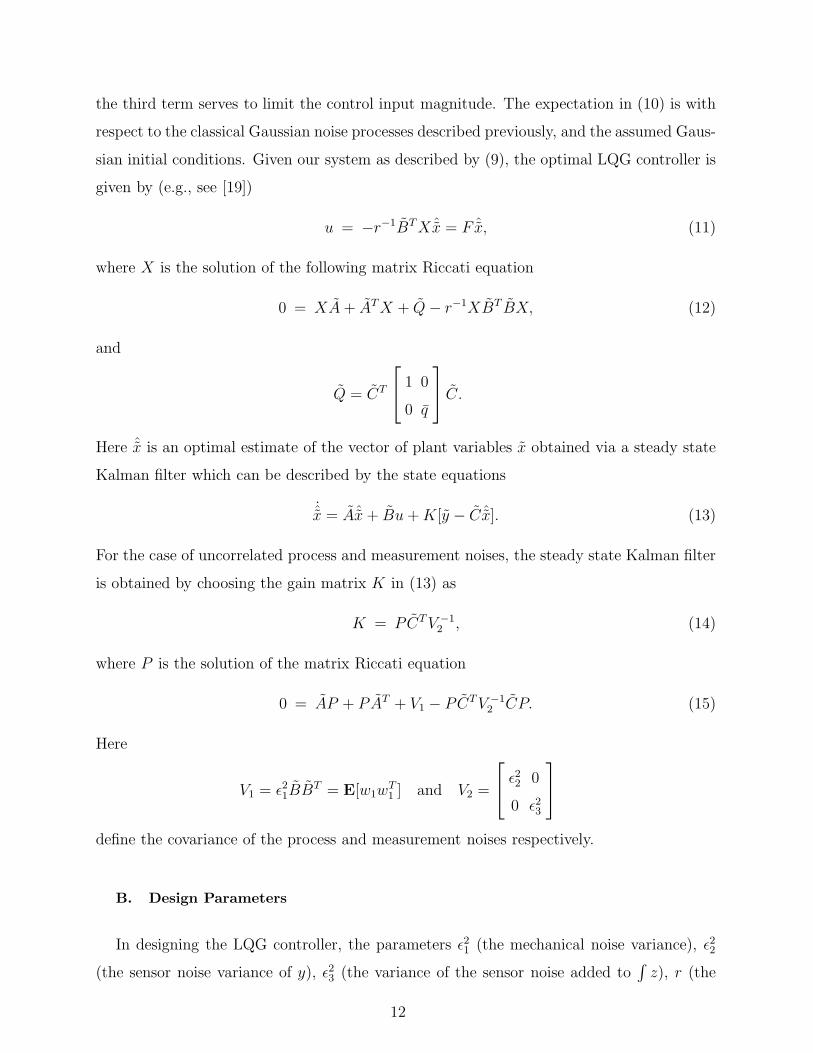
the third term serves to limit the control input magnitude. The expectation in (10) is with

respect to the classical Gaussian noise processes described previously, and the assumed Gaus-

sian initial conditions. Given our system as described by (9), the optimal LQG controller is

given by (e.g., see [19])

u = −r−1BT X ˆx = F ˆx, (11)

where X is the solution of the following matrix Riccati equation

0 = XA + AT X + Q − r−1XBT BX, (12)

and

Q = CT

1 0

0 q

C.

Here ˆx is an optimal estimate of the vector of plant variables x obtained via a steady state

Kalman filter which can be described by the state equations

˙x = Aˆx + Bu + K[y − C ˆx]. (13)

For the case of uncorrelated process and measurement noises, the steady state Kalman filter

is obtained by choosing the gain matrix K in (13) as

K = PCT V −1

2, (14)

where P is the solution of the matrix Riccati equation

0 = AP + PAT + V1 − PCTV −1

2CP. (15)

Here

V1 = ǫ2

1BBT = E[w1w

T1] and V2 =

ǫ2

20

0 ǫ2

3

define the covariance of the process and measurement noises respectively.

B. Design Parameters

In designing the LQG controller, the parameters ǫ2

1(the mechanical noise variance), ǫ2

2

(the sensor noise variance of y), ǫ2

3(the variance of the sensor noise added to

∫

z), r (the

12

control energy weighting in the LQG cost function) and q (the integral output weighting in

the LQG cost function) were used as design parameters and were adjusted for good controller

performance. This includes a requirement that the control system have suitable gain and

phase margins and a reasonable controller bandwidth. The specific values used for the design

are shown in Table I:

Design parameter Value

ǫ1 5 × 10−2

ǫ2 500

ǫ3 3 × 10−4

r 1 × 103

q 1 × 106

TABLE I: Design Parameter Values

These parameter values led to a 15th order LQG controller which is reduced to a 6th order

controller using a frequency-weighted balanced controller reduction approach. We reduce

the order of the controller to decrease the computational burden (and hence time-delay)

of the controller when it is discretized and implemented on a digital computer. The new

lower order model for the controller is determined via a certain controller reduction tech-

nique which minimizes the weighted frequency response error between the original controller

transfer function and the reduced controller transfer function; see [30]. This is illustrated in

Fig. 6 which shows Bode plots of the full-order controller and the reduced order controller.

Formally, the reduced order controller is constructed so that the quantity

∥

∥

∥

∥

P (s)C(s)

(I + P (s)C(s))(C(s) − Cr(s))

∥

∥

∥

∥

∞

(16)

is minimized. Here, P (s) = C(sI − A)−1B, is the plant transfer function matrix and

C(s) = F (sI − A + KC − BF )−1K is the original full controller transfer function matrix.

Also, Cr(s) is the reduced dimension controller transfer function matrix. The notation

‖M(s)‖∞ refers to the H∞ norm of a transfer function matrix M(s) which is defined to be

the maximum of σmax[M(iω)] over all frequencies ω ≥ 0. Here σmax[M(iω)] refers to the

maximum singular value of the matrix M(iω).

13

Note that this approach to controller reduction does not guarantee the stability of the

closed loop system with the reduced controller. We check for closed loop stability stability

separately after the controller reduction process.

10−1

100

101

102

103

104

105

−150

−100

−50

0

Mag

nitu

de(d

B)

FullReduced

10−1

100

101

102

103

104

105

−400

−300

−200

−100

0

100

Freq (Hz)

Pha

se(°

)

FIG. 6: Full and reduced-order continuous LQG controller Bode plots.

The reduced controller is then discretized at a sampling rate of 50 kHz and the cor-

responding Bode plot of the discrete-time loop gain is shown in Fig. 7. This discretized

controller provides good gain and phase margins of 16.2 dB and 63◦ respectively.

101

102

103

−100

−50

0

Mag

nitu

de(d

B)

Identified ModelTrue Plant with K

101

102

103

−1500

−1000

−500

0

Freq (Hz)

Pha

se(°

)

FIG. 7: Bode plot of loop gain L. The controller provides a gain margin of 16 dB and 63◦ phase

margin.

14

V. EXPERIMENTAL RESULTS

The discrete controller is implemented on a dSpace DS1103 Power PC DSP Board. This

board is fully programmable from a Simulink block diagram and possesses 16-bit resolution.

The controller successfully stabilizes the frequency in the optical cavity, locking its resonance

to that of the laser frequency, f0; see [31]. This can be seen from the experimentally

measured step response shown in Fig. 8 This step response was measured by applying a step

disturbance of magnitude 0.1 V to the closed-loop system as shown in Figure 9. Here r is

the step input signal and y is the resulting step response signal which was measured.

0 0.01 0.02 0.03 0.04 0.05 0.06 0.07 0.08 0.09 0.1−0.12

−0.1

−0.08

−0.06

−0.04

−0.02

0

0.02

Vol

tage

(V

)

Time (sec)

ExperimentalSimulated

FIG. 8: Step Response of the closed-loop system to an input of 0.1 V.

++

r

e

yPLANT

Controller

FIG. 9: Setup used to measure the closed-loop step response

15

VI. CONCLUSION AND FUTURE WORK

In this paper, we have shown that a systematic modern control technique such as LQG

integral control can be applied to a problem in experimental quantum optics which has

previously been addressed using traditional approaches to controller design. From frequency

response data gathered, we have successfully modeled the optical cavity system, and used

an extended version of the LQG cost functional to formulate the specific requirements of

the control problem. A controller was obtained and implemented which locks the resonant

frequency of the cavity to that of the laser frequency.

To improve on the current system, one might consider using additional actuators such as

a phase modulator situated within the cavity or an additional piezo actuator to control the

driving laser. Additional sensors which could be considered include using a beam splitter and

another homodyne detector to measure the other optical quadrature and an accelerometer

or a capacitive sensor to provide additional measurements of the mechanical subsystem.

In addition, it may be useful to control the effects of air turbulence within the cavity and

an additional interferometric sensor could be included to measure the optical path length

adjacent to the cavity. Such a measurement would be correlated to the air turbulence

effects within the cavity. All of these additional actuators and sensors could be expected to

improve the control system performance provided they were appropriately exploited using

a systematic multivariable control system design methodology such as LQG control.

One important advantage of the LQG technique is that it can be extended in a straight-

forward way to multivariable control systems with multiple sensors and actuators. Moreover,

the subspace approach to identification used to determine the plant is particularly suited to

multivariable systems. It is our intention to further the current work by controlling the laser

pump power using a similar scheme as the one used in this paper. This work is expected to

pave the way for extremely stable lasers with fluctuations approaching the quantum noise

limit and which could be potentially used in a wide range of applications in high precision

metrology, see [32].

[1] G. Milburn, Quantum Technology (Allen and Unwin, St Leonards, NSW, Australia, 1996).

[2] J. Dowling and G. Milburn, Proceedings of the Royal Society: Philosophical Transactions:

16

Mathematical, Physical and Engineering Sciences 361 (2003).

[3] V. Belavkin, Automation and Remote Control 42, 178 (1983).

[4] H. Mabuchi, in Proceedings of the 41st IEEE Conference on Decision and Control (Las Vegas,

Nevada, USA, 2002), pp. 450–451.

[5] H. Wiseman and G. Milburn, Physical Review Letters 70, 548 (1993).

[6] M. Armen, J. Au, J. Stockton, A. Doherty, and H. Mabuchi, Physical Review Letters 89

(2002), 133602.

[7] R. Ruskov, Q. Zhang, and A. Korotkov, in Proceedings of the 42nd IEEE Conference on

Decision and Control (Maui, Hawaii, USA, 2003), pp. 4185–4190.

[8] A. Doherty and K. Jacobs, Physical Review A 60, 2700 (1999).

[9] S. Haine, A. Ferris, J. Close, and J. Hope, Phys. Rev. A 69, 013605 (2004).

[10] H. Wiseman, Physical Review Letters 75, 4587 (1995).

[11] C. Ahn, A. Doherty, and A. Landahl, Physical Review A 65 (2002), 042301.

[12] J. Stockton, J. Geremia, A. Doherty, and H. Mabuchi (2003), quant-ph/0309101.

[13] M. Yanagisawa and H. Kimura, IEEE Transactions on Automatic Control 48, 2107 (2003).

[14] M. Yanagisawa and M. R. James, in Proceedings of the 17th IFAC World Congress (Seoul,

Korea, 2008).

[15] A. Hopkins, K. Jacobs, S. Habib, and K. Schwab, Physical Review B 68 (2003).

[16] S. C. Edwards and V. P. Belavkin, quant-ph/0506018, University of Nottingham (2005).

[17] M. R. James, H. I. Nurdin, and I. R. Petersen, IEEE Transactions on Automatic Control

(2008), to Appear.

[18] H. Mabuchi, arXiv:0803.2007v1 [quant-ph], Stanford University (2008).

[19] H. Kwakernaak and R. Sivan, Linear Optimal Control Systems (Wiley, 1972).

[20] M. J. Grimble, Proceedings of the IEE, Part D 126, 841 (1979).

[21] T. McKelvey, H. Akcay, and L. Ljung, IEEE Transactions on Automatic Control 41, 960

(1996).

[22] H. Bachor and T. Ralph, A Guide to Experiments in Quantum Optics (Wiley-VCH, Weinheim,

Germany, 2004), 2nd ed.

[23] C. Gardiner and P. Zoller, Quantum Noise (Springer, Berlin, 2000).

[24] A. E. Siegman, Lasers (University Science, Mill Valley, CA, 1986).

[25] R. C. Dorf and R. H. Bishop, Modern Control Systems, 7 Ed. (Addison-Wesley, Reading,

17

Massachusetts, 1995).

[26] P. van Overschee and B. De Moor, Subspace Identification for Linear Systems (Kluwer Aca-

demic Publishers, 1996).

[27] K. J. Astrom, Introduction to Stochastic Control Theory (Academic Press, New York, 1970).

[28] B. D. O. Anderson and J. B. Moore, Optimal Control: Linear Quadratic Methods (Prentice-

Hall, 1990).

[29] Y.-J. Cheng, IEEE Journal of Quantum Electronics 30, 1498 (1994).

[30] K. Zhou, J. Doyle, and K. Glover, Robust and Optimal Control (Prentice-Hall, Upper Saddle

River, NJ, 1996).

[31] S. Z. S. Hassen, E. H. Huntington, M. R. James, and I. R. Petersen, in Proceedings of the 17th

IFAC World Congress (Seoul, Korea, 2008).

[32] E. H. Huntington, C. C. Harb, M. Heurs, and T. C. Ralph, Phys. Rev. A 75, 013802 (2007).

18