On the construction of local quadratic spline quasi-interpolants on bounded rectangular domains
Upload
independentCategory
view
2download
0
SIAM J. CONTROL AND OPTIMIZATION c° 2000 Society for Industrial and Applied Mathematics
Vol. 0, No. 0, pp. 000{000, Month 2000 000
A TWOFOLD SPLINE APPROXIMATION FOR FINITE HORIZONLQG CONTROL OF HEREDITARY SYSTEMS *
ALFREDO GERMANIy, COSTANZO MANESy, AND PIERDOMENICO PEPEy
Abstract. In this paper an approximation scheme is developed for the solution of the LinearQuadratic Gaussian (LQG) control on a ¯nite time interval for Hereditary Systems with multiplenoncommensurate delays and distributed delay. The solution here proposed is achieved by meansof two approximating subspaces: the ¯rst one to approximate the Riccati equation for control andthe second one to approximate the ¯ltering equations. Since the approximating subspaces have ¯nite
dimension, the resulting equations can be implemented. The convergence of the approximated controllaw to the optimal one is proved. Simulation results are reported on a wind tunnel model, showingthe high performance of the method.
Key words. Hereditary Systems, Linear Quadratic Gaussian Regulator, In¯nite DimensionalSystems, Galerkin Spline Approximation
AMS subject classi¯cations. 93E11, 93E20, 93E25
1. Introduction. It is well known that the solution of the Linear QuadraticRegulation problem and of the optimal Gaussian Filtering problem for linear DelaySystems is found in term of in¯nite dimensional operators. On the other hand, im-plementation of a control/¯ltering scheme in this case requires a ¯nite dimensionalapproximation of such operators.
Although much attention has been devoted to separately develop an approxima-tion theory for the Linear Quadratic Regulation [4,11,12,24,26,27,30,40] and for theoptimal Gaussian Filtering [14,20] of Delay Systems, the approximation problem ofthe overall Linear Quadratic Gaussian Regulator has not been conveniently treated inliterature.
The averaging approximation scheme has been used in [24], for both the ¯nite andin¯nite horizon LQ problem of Delay Systems, and convergence results are obtainedby considering a conjecture, later proved to be true [41], that is the question whetherthe sequence of approximating systems gives uniformly exponentially stable systemsfor su±ciently large indexes, if the underlying retarded functional di®erential equationis stable.
The spline approximation scheme developed in [3] has been applied to the LQProblem of Delay Systems in [4]. Although numerical simulations show better per-formance than the averaging scheme, no theoretical convergence results are so faravailable. In [6], it is proved that the adjoint of the approximate semigroup governingthe system does not converge in a strong way to the adjoint of such semigroup. Asa consequence, the main hypothesis which guarantees the convergence results in [24]cannot be satis¯ed, and therefore this spline approximation scheme cannot be safelyapplied.
A new spline approximation scheme has been developed in [27], for the LQ prob-lem of Delay Systems with any number of pure delay terms, assuming the absolute
*Received by the editors April 16, 1998; accepted by the editors July 6, 2000. This work wassupported by ASI (Agenzia Spaziale Italiana)..
yDipartimento di Ingegneria Elettrica dell'Universitµa degli Studi dell'Aquila, 67040 Montelucodi Roio, L'Aquila, Italy, (fgermani,manes,[email protected]).
1

2 ALFREDO GERMANI, COSTANZO MANES, AND PIERDOMENICO PEPE
continuity of the kernel in the distributed delay integral. Theoretical convergence re-sults are obtained in the ¯nite horizon case, as this approximation scheme does notguarantee the uniform exponential stability of the approximate semigroups. How-ever, it is proved in [28,29] that, in the case of commensurate delays and withoutdistributed delay, a weaker condition is su±cient to obtain the strong convergenceof the approximated LQ algebraic Riccati Equation solution. The authors call thiscondition uniform output stability. It is proved that the spline approximation schemedeveloped in [27] does satisfy this condition, so that the above convergence result isavailable, for the in¯nite horizon case. But, as pointed out by Morris in page 9 ofpaper [36], the convergence properties of this approximation scheme are not su±cientto ensure convergence of the closed loop response.
In [40], a piecewise linear approximation theory has been developed for the ¯niteand in¯nite horizon LQ of general Delay Systems. Theoretical convergence resultsare obtained both in the ¯nite and in¯nite horizon cases, as the condition of uniformexponential stability is veri¯ed.
In [32] error estimates are established for the approximation of Delay Systemsby means of the averaging scheme. In [26] a scheme using ¯rst-order splines is devel-oped satisfying the uniform exponential stability condition, and error estimates areestablished too, as it is done in [32] for the averaging scheme. Such a scheme usesthe classic averaging subspace of piecewise constant functions where to de¯ne the ap-proximated system equation, but de¯nes the approximated in¯nitesimal generator inthat subspace not in the usual averaging methodology but using an inverse projectorfrom such subspace to the subspace built up using splines. Such a scheme, which isa mixed averaging spline one, is used in [26] for the in¯nite horizon LQ problem ofgeneral hereditary systems.
The matter of uniform exponential stability for spline approximation schemeshas been investigated in [15], in the scalar open loop case. There the real eigenvalue(unique if the coe±cient on delay term is positive, in the hereditary equation) ofthe in¯nitesimal generator of the semigroup governing the system is used, in orderto de¯ne a particular inner product, by which Galerkin spline approximations [3]preserve the uniform exponential stability of the approximated semigroups. How thiscan be applied to optimal multivariable regulator problems is an open and interestingquestion.
In the synthesis of approximate optimal controllers developed by all above ap-proximation schemes [4,24,26,27,40] it is assumed that the system state is completelyaccessible. Moreover the approximated control input is generated by a ¯nite rankfeedback operator applied to the true state in the delay time interval. From an engi-neering point of view, the resulting controller is still in¯nite dimensional and thereforenot directly implementable.
The synthesis of ¯nite dimensional dynamic output feedback compensators forhereditary systems in a deterministic setting is considered in paper [25], section 4.2.The proposed controller is composed of an observer and of a feedback control law fromthe observed state. Both the gains, for the ¯nite dimensional observer and control,are obtained by approximating the solutions of two algebraic Riccati equations. Theresulting controller resembles the solution of an LQG problem, although no referenceto an optimal stochastic control problem is made in the paper. The main tool is theuse of the averaging approximation scheme [2,24] and the main result is the stabilityof the overall closed loop system.
In [35] the same problem is investigated with reference to a general class of de-terministic distributed systems.

SPLINE APPROXIMATION FOR LQG CONTROL OF HEREDITARY SYSTEMS 3
An approximation theory, that provides an implementable scheme, for the ¯lteringproblem of systems evolving on Hilbert Spaces has been studied in [14,20]. This theoryhas been successfully applied to Delay Systems.
In literature the case with one pure delay term is usually completely reported,[2,24,28,29,40] and the general case with multiple noncommensurate delays is usuallyjust brie°y indicated. However, the extension of all results to such general case is notstraightforward [2,3,24,40] or even infeasible [28,29].
As a ¯nal point of this bibliographic review, it must be stressed the existence ofa large amount of spline approximation schemes [3,4,26,27,40] for the deterministicoptimal quadratic state regulator (LQ problem), where the control gain operator isapproximated by approximating the relevant Riccati Equation. In principle, the sameapproximation schemes could be adapted for approximating the covariance operatorde¯ned by the solution of the dual Riccati Equation, and the Kalman Filter Equation,that solve the LQG problem in the stochastic setting. On the other hand, the applica-bility of such schemes to the case of stochastic Delay Systems with partial noisy stateobservations is not a trivial question and it has not been investigated up to now, andthe main problem of proving the convergence remains unsolved.
The control problem with partial state observation has been treated in literatureemploying the averaging scheme in a deterministic setting [25]. On the other hand itis a known result [4] the superiority of spline approximation schemes with respect toaveraging ones, with respect to numerical convergence rate.
On the basis of these considerations the aim of this paper is to de¯ne a ¯-nite dimensional scheme that approximates the solution of the Finite Horizon Lin-ear Quadratic Gaussian Control problem for Stochastic Delay Systems with partialobservations. The resulting implementable scheme has the following features:
(i) the optimal closed loop response of the LQG problem can be approximatedwith arbitrarily small error;
(ii) the scheme can be applied also in the LQ problem;(iii) the approximation method is based on splines and not on averaging;(iv) the matrices that implement the approximation of the optimal ¯lter-controller
scheme are easily parameterized as a function of the approximation order, and can beeasily computed;
(v) the scheme allows to deal with general hereditary systems, that is withmultiple noncommensurate delays and distributed delay;
(vi) simultaneous approximation of a semigroup and of its adjoint is not required,so that problems arising from non density of the intersection of the respective generatordomains are avoided;
(vii) the scheme allows a quite natural extension to be used for the solution of thein¯nite horizon LQG problem;(viii) the scheme has nice numerical properties, in that it shows good performances
even with a low ¯nite dimensional approximation order;(ix) the scheme allows to get a faster convergence of the approximation by in-
creasing the order of the spline degree.Of course for most of the above mentioned points, the scienti¯c literature o®ers
e®ective algorithms. Nevertheless, the problem of considering at the same time allthese issues remains an interesting point.
The paper is organized as follows. In section 2 Stochastic Hereditary Systemsare written in state-space form and the in¯nitesimal generator of the adjoint of thesemigroup that governs the system is studied. It is proved that such operator hasa deeply di®erent structure if a weighted inner product is used instead of the usual
4 ALFREDO GERMANI, COSTANZO MANES, AND PIERDOMENICO PEPE
one. In section 3 the ¯nite horizon LQG is presented, and theorems for a suitable ap-proximation scheme are proved. In section 4 an approximation scheme which satis¯eshypotheses of section 3 is described for the general case. In section 5 matrices whichrepresent ¯nite dimensional linear operators are calculated to implement the method.In section 6 the in¯nite horizon case is addressed. In section 7 simulation results arereported, showing the e®ectiveness of the proposed method. Section 8 contains theconclusions.
2. Stochastic Delay Systems. In this paper we deal with the class of thosedynamical systems that in technical literature are generally known as linear delaysystems, sometimes also called hereditary systems. When state and observation noiseare present, these are described, for t ¸ 0, by stochastic equations of the type
(2.1)
_z(t) = A0z(t) +±X
h=1
Ahz(t¡ rh)
+
Z 0
¡rA01(#)z(t+ #)d#+B0u(t) + F0!(t);
y(t) = C0z(t) +G!(t);
with z(t) 2 IRN , u(t) 2 IRp, y(t) 2 IRq, !(t) 2 IRs, r± = r > r±¡1 > ¢ ¢ ¢ r1 > r0 = 0,Ah 2 IRN£N , A01 2 L2([¡r; 0]; IRN£N ), B0 2 IRN£p, C0 2 IRq£N , G 2 IRq£s,F0 2 IRN£s.
The noise ! belongs to the Hilbert space L2([0; tf ]; IRs) equipped with the stan-
dard Gaussian cylinder measure (this corresponds to model ! as a white-noise process[1]). Independence of state and observation noises is assumed, that is F0GT = 0 and,without loss of generality, GGT = Iq, where Iq denotes the identity matrix in IR
q£q.The variable z in the interval [¡r; 0] is assumed to be generated as follows
(2.2) z(#) = ¹z(#) +
Z 0
¡rk(#; ¿)¹!(¿)d¿; # 2 [¡r; 0];
where ¹z is absolutely continuous with derivative in L2([¡r; 0]; IRN) and the process¹!, independent of !, belongs to the Hilbert space L2([¡r; 0]; IR¹s) equipped with thestandard Gaussian cylinder measure, and the kernel k(#; ¿) is integrable for ¿ 2 [¡r; 0].
As well known, system (2.1) can be rewritten in state-space form in the HilbertSpaceM2 = IR
N£L2([¡r; 0]; IRN ), endowed with the following weighted inner product[3]:
(2.3)
µ·x0x1
¸;
·y0y1
¸¶M2
= xT0 y0 +
Z 0
¡rxT1 (#)y1(#)g(#)d#;
where g(#) is the piecewise constant non-decreasing function de¯ned as
(2.4) g(#) = Â[¡r±;¡r±¡1](#) +±¡1Xj=1
(± ¡ j + 1)Â(¡rj ;¡rj¡1](#);
where ÂS denotes the characteristic function of the interval S.Here and in the following the standard assumption is made that summations
vanish when the upper limit is smaller than the lower one (e. g. ± = 1 in (2.4)).

SPLINE APPROXIMATION FOR LQG CONTROL OF HEREDITARY SYSTEMS 5
In the paper, for the sake of brevity and whenever it does not cause confusion,the space L2([¡r; 0]; IRN ) will be simply indicated as L2. In the same way Ck willdenote the space Ck([¡r; 0]; IRN ) of functions with values in IRN that have continuousderivatives until order k, while the symbol W 1;2 will indicate the space of absolutelycontinuous functions from [¡r; 0] in IRN , with derivative in L2.
InM2 the system (2.1), (2.2) assumes the form
_x(t) = Ax(t) +Bu(t) + F!(t); x(0) =
·¹z(0)¹z
¸+
·L0L1¸¹!;(2.5)
y(t) = Cx(t) +G!(t);(2.6)
where A : D(A)7!M2 is de¯ned as
(2.7) A
·x0x1
¸=
24A0x0 +P±
h=1Ahx1(¡rh)+R 0¡rA01(#)x1(#)d#
d
d#x1
35with domain
(2.8) D(A) =(·x0x1
¸ ¯ x0 2 IRNx1 2W 1;2
x0 = x1(0)
);
and the linear operators B;C;F are de¯ned as
(2:9) B : IRp 7!M2; Bu(t) =
·B0u(t)0
¸;
(2:10) C :M2 7! IRq; C
·x0x1
¸= C0x0;
(2:11) F : IRs 7!M2; F!(t) =
·F0 !(t)0
¸:
The Hilbert-Schmidt operator L =·L0L1¸, that de¯nes the stochastic initial state x(0),
derives from de¯nition (2.2) and is de¯ned as follows
(2:12)
L0 : L2([¡r; 0]; IR¹s)7! IRN ; L0! =Z 0
¡rk(0; ¿)¹!(¿)d¿;
L1 : L2([¡r; 0]; IR¹s)7!W 1;2; L1!(#) =Z 0
¡rk(#; ¿)¹!(¿)d¿:
The mean value and nuclear covariance of the initial state x0 are as follows
(2:13) ¹x0 =
·¹z(0)¹z
¸; P0 = LL¤:
Remark 2.1. Note that the weighted scalar product (2.3), (2.4) assures thatthere exist real ® such that A ¡ ®I has the nice property to be dissipative [3]. Thisproperty is used in the paper to prove the convergence of the approximation scheme.
6 ALFREDO GERMANI, COSTANZO MANES, AND PIERDOMENICO PEPE
For reader convenience the de¯nitions of some operators related to the system(2.5), (2.6) that will be extensively used in the paper, are reported below.
Proposition 2.2. The operators B¤, C¤, F ¤, BB¤, C¤C, FF ¤ and A¤ areas follows
B¤ :M2 7! IRp; B¤·x0x1
¸= BT
0 x0;(2.14)
C¤ : IRq 7!M2; C¤y =·CT0 y0
¸;(2.15)
F ¤ :M2 7! IRs; F ¤·x0x1
¸=
·FT0 x00
¸;(2.16)
BB¤ :M2 7!M2; BB¤·x0x1
¸=
·B0BT
0 x00
¸;(2.17)
C¤C :M2 7!M2; C¤C·x0x1
¸=
·CT0 C0x00
¸;(2.18)
FF ¤ :M2 7!M2; FF ¤·x0x1
¸=
·F0FT0 x0
0
¸;(2.19)
(2.20)
A¤ : D(A¤)7!M2;
A¤·y0y1
¸=
264 ± y1(0) +AT0 y0
1
gAT01y0 ¡
d
d#
³y1 ¡
±¡1Xj=1
kj(y0;y1)Â[¡r;¡rj ]´375 ;
with dense domain
(2.21) D(A¤) =
8<:24y0y1
35 ¯ y0 2 IRN ; AT± y0 = y1(¡r);³
y1 ¡P±¡1j=1 kj(y0;y1)Â[¡r;¡rj ]
´2W 1;2
9=;where
(2.22) kj(y0;y1) =y1(¡rj)¡AT
j y0
± ¡ j + 1 ; j = 1; : : : ; ± ¡ 1:
The proof that the operator de¯ned by (2.20), (2.21), (2.22), is in fact the adjointof operator A is reported in Appendix.
Remark 2.3. The di®erence between the case of just one pure delay and ofmultiple pure delays is given by summations in (2.20), (2.21), which vanish in the ¯rstcase and complicate so much the analysis in the second one.
3. The ¯nite horizon LQG for delay systems. In this section the problem ofde¯ning a feedback control law for the stochastic delay system (2.1) (2.2) is considered.In particular we are interested in the problem of synthesizing the control law thatminimizes the cost functional
(3.1) Jf (u) =
Z tf
0
E[zT(t)Q0z(t) + uT(t)u(t)]dt;

SPLINE APPROXIMATION FOR LQG CONTROL OF HEREDITARY SYSTEMS 7
with 0 < tf < 1, where matrix Q0 is symmetric non negative de¯nite. It can bereadily recognized that the functional (3.1) admits the following representation inM2
(3.2) Jf (u) =
Z tf
0
E[¡Qx(t);x(t)
¢+ uT(t)u(t)]dt;
where Q :M2 7!M2 is de¯ned as
(3:3) Q
·x0x1
¸=
·Q0x00
¸and x(t) satis¯es system equations (2.5) (2.6). The solution of this problem is, as wellknown, the classical LQG controller, given by the following equations [1]:
u(t) = ¡B¤R(tf ¡ t)x(t)(3.4)
R(t) =
Z t
0
T ¤(t¡ ¿)[Q¡R(¿)BB¤R(¿)]T (t¡ ¿)d¿(3.5)
x(t) = T (t)x0 +
Z t
0
T (t¡ ¿) [P (¿)C¤[y(¿)¡Cx(¿)] +Bu(¿)] d¿(3.6)
P (t) = T (t)P0T ¤(t) +Z t
0
T (t¡ ¿)[FF ¤ ¡P (¿)C¤CP (¿)]T ¤(t¡ ¿)d¿(3.7)
where T (t) is the semigroup governing the system, that is the semigroup generatedby the operator A in (2.7) (2.8), and x0 and P0 are the expected value and thecovariance operator of the initial state x(0) in M2, respectively. The solution givenby these equations is a very important result only from a theoretical point of view.For our purposes we need to recall that the solutions of the Riccati Equations (3.5)(3.7) evolve in the Hilbert Space of Hilbert Schmidt operators and moreover, for everytf <1, there exist constants KP and KR such that [20]
(3:8)
supt2[0;tf ]
kP (t)kH:S: = KP <1;
supt2[0;tf ]
kR(t)kH:S: = KR <1:
where, as usual, k ¢ kH:S: denotes the Hilbert-Schmidt norm [1].In engineering applications, due to its in¯nite dimensional nature, such a solution
is not directly implementable. Therefore it becomes important to investigate whensuch a solution admits a ¯nite dimensional approximation.
Throughout the paper, given a Hilbert space X and a closed subspace S ½ X ,the orthogonal projection operator from X to S will be denoted as ¦S .
In the next Lemma, that is proved in [20], the linear space of bounded operatorson a Hilbert Space H is denoted L(H).
Lemma 3.1. Let H1; H2 be separable Hilbert Spaces. Let fGm(t); t 2 [0; tf ]gbe a sequence of strongly continuous L(H2) valued functions, strongly convergent tofG(t); t 2 [0; tf ]g, uniformly on [0; tf ]. Let K be a compact subset in the Hilbert Spaceof Hilbert-Schmidt operators mapping H1 to H2.
Then kGm(t)N ¡G(t)NkH:S: converges to zero, uniformly with respect to N 2 Kand t 2 [0; tf ].

8 ALFREDO GERMANI, COSTANZO MANES, AND PIERDOMENICO PEPE
Lemma 3.2. Let H1 and H2 be separable Hilbert Spaces. Let G(t) be a semigroupon H2 and Gn(t) a sequence of semigroups on H2 strongly convergent to G(t) uniformlywith respect to t 2 [0; tf ]. For 0 · ¿ · t, let ¡(t; ¿) be the mild evolution operator
(3:9) ¡(t; ¿) = G(t¡ ¿) +Z t
¿
G(t¡ #)Op(#)¡(#; ¿)d#;
where Op 2 C ([0; tf ];L(H2)) and let ¡n(t; ¿) be the sequence of mild evolution opera-tors
(3:10) ¡n(t; ¿) = Gn(t¡ ¿) +Z t
¿
Gn(t¡ #)Opn(#)¡n(#; ¿)d#;
where Opn 2 C ([0; tf ];L(H2)) converges pointwise strongly to Op, uniformly in [0; tf ].Let K be a compact subset in the Hilbert Space of Hilbert-Schmidt operators mappingH1 to H2.
Then k¡(t; ¿)N¡¡n(t; ¿)NkH:S: converges to zero, uniformly with respect to N 2K and 0 · ¿ · t · tf :
Proof. It is
(3:11)
k¡(t; ¿)N ¡ ¡n(t; ¿)NkH:S:· kG(t¡ ¿)N ¡Gn(t¡ ¿)NkH:S:+
Z t
¿
kG(t¡ #)Op(#)k ¢ k¡(#; ¿)N ¡ ¡n(#; ¿)NkH:S:d#
+
Z t
¿
kG(t¡ #)Op(#)¡Gn(t¡ #)Opn(#)k¢ k¡n(#; ¿)N ¡ ¡(#; ¿)NkH:S:d#
+
Z t
¿
k(G(t¡ #)Op(#)¡Gn(t¡ #)Opn(#))¡(#; ¿)NkH:S:d#:
Let M a positive real such that
(3:12)
M ¸ sup(t;#)2[0;tf ]£[0;tf ]
kG(t)kkOp(#)k;
M ¸ sup(t;#;n)2[0;tf ]£[0;tf ]£Z+
kGn(t)kkOpn(#)k:
Then
(3:13)
k¡(t; ¿)N ¡ ¡n(t; ¿)NkH:S: · kG(t¡ ¿)N ¡Gn(t¡ ¿)NkH:S:+
Z t
¿
k(G(t¡ #)Op(#)¡Gn(t¡ #)Opn(#))¡(#; ¿)NkH:S:d#
+ 3M
Z t
¿
k¡¡n(#; ¿)¡ ¡(#; ¿)¢NkH:S:d#:

SPLINE APPROXIMATION FOR LQG CONTROL OF HEREDITARY SYSTEMS 9
Applying the Gronwall's inequality
(3:14)
k¡(t; ¿)N ¡ ¡n(t; ¿)NkH:S: · e3Mtf
³kG(t¡ ¿)N ¡Gn(t¡ ¿)NkH:S:
+
Z t
¿
°°¡G(t¡ #)Op(#)¡Gn(t¡ #)Opn(#)¢¡(#; ¿)N°°H:S:d#´· e3Mtf
³kG(t¡ ¿)N ¡Gn(t¡ ¿)NkH:S:
+
Z t
¿
°°¡G(t¡ #)¡Gn(t¡ #)¢Op(#)¡(#; ¿)N°°H:S:d#+
Z t
¿
M°°¡Op(#)¡Opn(#)¢¡(#; ¿)N°°H:S:d#´:
Since the set of operators fOp(#)¡(t; ¿)N; # 2 [0; tf ]; 0 · ¿ · t · tfg and the setf¡(t; ¿)N; 0 · ¿ · t · tfg are compact in the Hilbert space of Hilbert-Schmidt oper-ators mapping H1 to H2, by Lemma 3.1 the right hand side of inequality (3.14) tendsto zero for n!1, and the Lemma is proved.
Theorem 3.3. Let ªn and ª0n be sequences of ¯nite dimensional subspaces ofM2 contained in D(A) and in D(A¤), respectively. Let ¦ªn :M2 7! ªn and ¦ª0
n:
M2 7! ª0n be the sequences of ortho-projection operators in ªn and ª0n, respectively.Let Tªn(t) be the semigroup generated by the operator ¦ªnA¦ªn : M2 7! ªn andT ¤ª0
n(t) the semigroup generated by the operator ¦ª0
nA¤¦ª0
n:M2 7! ª0n. Let Pn(t)
and Rn(t) be the solutions of the ¯nite dimensional di®erential Riccati equations
_Pn(t) =¦ªnA¦ªnPn(t) +Pn(t)(¦ªnA¦ªn)¤
¡Pn(t)¦ªnC¤C¦ªnPn(t) +¦ªnFF ¤¦ªn ;(3.15)
Pn(0) =¦ªnP0¦ªn ;
_Rn(t) =¦ª0nA¤¦ª0
nRn(t) +Rn(t)(¦ª0
nA¤¦ª0
n)¤
¡Rn(t)¦ª0nBB¤¦ª0
nRn(t) +¦ª0
nQ¦ª0
n;(3.16)
Rn(0) = 0
Assume the following hypotheses are satis¯ed:
Hp1) ¦ªn converges strongly to the identity operator ;
Hp2) ¦ª0nconverges strongly to the identity operator ;
Hp3) Tªn(t) converges strongly to T (t) uniformly in [0; tf ];
Hp4) T ¤ª0n(t) converges strongly to T ¤(t) uniformly in [0; tf ].
Then
(3:17)kPn(t)¡¦ªnP (t)¦ªnkH:S: ! 0;
kRn(t)¡¦ª0nR(t)¦ª0
nkH:S: ! 0;
uniformly in [0; tf ]:
Proof. See the proof of Theorem 3 in [20].Remark 3.4. Note that, with the given de¯nitions, in general the semigroup
T ¤ª0n(t) generated by the operator ¦ª0
nA¤¦ª0
nis di®erent from the semigroup T ¤ªn
(t),the adjoint of the semigroup generated by ¦ªnA¦ªn .
10 ALFREDO GERMANI, COSTANZO MANES, AND PIERDOMENICO PEPE
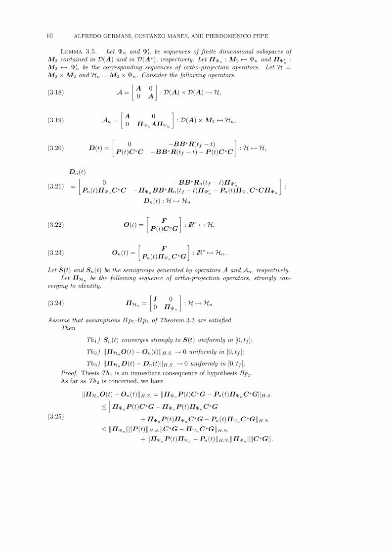
Lemma 3.5. Let ªn and ª0n be sequences of ¯nite dimensional subspaces ofM2 contained in D(A) and in D(A¤), respectively. Let ¦ªn :M2 7! ªn and ¦ª0
n:
M2 7! ª0n be the corresponding sequences of ortho-projection operators. Let H =M2 £M2 and Hn =M2 £ªn. Consider the following operators
(3:18) A =·A 00 A
¸: D(A)£D(A)7!H;
(3:19) An =·A 00 ¦ªnA¦ªn
¸: D(A)£M2 7!Hn;
(3:20) D(t) =
·0 ¡BB¤R(tf ¡ t)
P (t)C¤C ¡BB¤R(tf ¡ t)¡P (t)C¤C
¸: H7!H;
(3:21)
Dn(t)
=
·0 ¡BB¤Rn(tf ¡ t)¦ª0
n
Pn(t)¦ªnC¤C ¡¦ªnBB¤Rn(tf ¡ t)¦ª0n¡Pn(t)¦ªnC¤C¦ªn
¸:
Dn(t) : H7!Hn
(3:22) O(t) =
·F
P (t)C¤G
¸: IRs 7!H;
(3:23) On(t) =
·F
Pn(t)¦ªnC¤G
¸: IRs 7!Hn:
Let S(t) and Sn(t) be the semigroups generated by operators A and An, respectively.Let ¦Hn be the following sequence of ortho-projection operators, strongly con-
verging to identity,
(3:24) ¦Hn =
·I 00 ¦ªn
¸: H7!Hn
Assume that assumptions Hp1-Hp4 of Theorem 3.3 are satis¯ed.Then
Th1) Sn(t) converges strongly to S(t) uniformly in [0; tf ];
Th2) k¦HnO(t)¡On(t)kH:S: ! 0 uniformly in [0; tf ];
Th3) k¦HnD(t)¡Dn(t)kH:S: ! 0 uniformly in [0; tf ].
Proof. Thesis Th1 is an immediate consequence of hypothesis Hp3.As far as Th2 is concerned, we have
(3:25)
k¦HnO(t)¡On(t)kH:S: = k¦ªnP (t)C¤G¡ Pn(t)¦ªnC¤GkH:S:·°°°¦ªnP (t)C¤G¡¦ªnP (t)¦ªnC¤G
+¦ªnP (t)¦ªnC¤G¡Pn(t)¦ªnC¤GkH:S:· k¦ªnkkP (t)kH:S:kC¤G¡¦ªnC¤GkH:S:
+ k¦ªnP (t)¦ªn ¡Pn(t)kH:S:k¦ªnkkC¤Gk:

SPLINE APPROXIMATION FOR LQG CONTROL OF HEREDITARY SYSTEMS 11
From (3.25) it follows that k¦HnO(t) ¡ On(t)kH:S: ! 0 uniformly with respect tot 2 [0; tf ], because of the boundedness of kP (t)kH:S and the uniform convergence ofPn(t) stated in Theorem 3.3.
As for thesis Th3, it is
(3:26) ¦HnD(t)¡Dn(t) =
·0 Opn1;2(t)
Opn2;1(t) Opn2;2(t)
¸;
where
Opn1;2(t) = BB¤Rn(tf ¡ t)¦ª0
n¡BB¤R(tf ¡ t);
Opn2;1(t) =¦ªnP (t)C¤C ¡Pn(t)¦ªnC¤C;(3:27)
Opn2;2(t) =¦ªnBB¤Rn(tf ¡ t)¦ª0n
+Pn(t)¦ªnC¤C¦ªn ¡¦ªnBB¤R(tf ¡ t)¡¦ªnP (t)C¤C:
To prove Th3 it is su±cient to prove that the three operators in (3.27) convergeuniformly to zero in the H:S: norm. Let us start with operator Opn1;2(t). We have
(3.28)kOpn1;2(t)k · kBB¤k°°Rn(tf ¡ t)¡¦ª0
nR(tf ¡ t)¦ª0
n
°°H:S:
k¦ª0nk
+ kBB¤k°°¦ª0nR(tf ¡ t)¦ª0
n¡R(tf ¡ t)
°°H:S:
:
Moreover, from the uniform convergence of Rn(t) stated in Theorem 3.3, being R selfadjoint, and for Lemma 3.1, by
(3:29)
k¦ª0nR(tf ¡ t)¦ª0
n¡R(tf ¡ t)kH:S:
· k¦ª0nR(tf ¡ t)¦ª0
n¡R(tf ¡ t)¦ª0
n+R(tf ¡ t)¦ª0
n¡R(tf ¡ t)kH:S:
· 2k¦ª0nR(tf ¡ t)¡R(tf ¡ t)k
it follows that kOpn1;2(t)kH:S: ! 0 uniformly in [0; tf ]. Consider now the termOpn2;1(t). Its Hilbert-Schmidt norm satis¯es
(3:30)
kOpn2;1(t)kH:S:· °°¦ªnP (t)¡¦ªnP (t)¦ªn +¦ªnP (t)¦ªn ¡Pn(t)¦ªn
°°H:S:
kC¤Ck·³kP (t)¡P (t)¦ªnkH:S: + k(¦ªnP (t)¦ªn ¡Pn(t))¦ªnkH:S:
´kC¤Ck:
Since, by Lemma 3.1, k¦ªnP (t) ¡ P (t)kH:S: ! 0 uniformly and k(¦ªnP (t)¦ªn ¡Pn(t))¦ªnkH:S: ! 0 by Theorem 3.3, it follows that the norm of Opn2;1(t) tends tozero uniformly in [0; tf ].
It remains to prove that kOpn2;2(t)kH:S: ! 0 uniformly.
(3:31)kOpn2;2(t)kH:S: · k¦ªnk
°°BB¤R(tf ¡ t)¡BB¤Rn(tf ¡ t)¦ª0n
°°H:S:
+°°¦ªnP (t)C¤C ¡Pn(t)¦ªnC¤C¦ªn
°°H:S:
Uniform convergence to zero of kBB¤R(tf¡t)¡BB¤Rn(tf¡t)¦ª0nkH:S: has already
been proved. Moreover
(3:32)
k¦ªnP (t)C¤C ¡Pn(t)¦ªnC¤C¦ªnkH:S:· k¦ªnkkP (t)C¤C ¡P (t)¦ªnC¤C¦ªnkH:S:
+°°¡¦ªnP (t)¦ªn ¡Pn(t)
¢¦ªnC¤C
°°H:S:
k¦ªnk:

12 ALFREDO GERMANI, COSTANZO MANES, AND PIERDOMENICO PEPE
Again, as proved in [20] the term k(¦ªnP (t)¦ªn ¡ Pn(t))¦ªnkH:S: ! 0 uniformlyand thanks to Lemma 3.1 also kC¤CP (t)¡¦ªnC¤C¦ªnP (t)kH:S: ! 0 uniformly.From (3.32) it follows that k¦ªnP (t)C¤C¡Pn(t)¦ªnC¤C¦ªnkH:S: ! 0 uniformly,so that kOpn2;2(t)kH:S: ! 0 uniformly in [0; tf ], and the Lemma is proved.
Lemma 3.6. Let U(t; ¿); 0 · ¿ · t, be the mild evolution operator
(3:33) U(t; ¿) = S(t¡ ¿) +Z t
¿
S(t¡ #)D(#)U(#; ¿)d#:
Let fUn(t; ¿)g be the sequence of mild evolution operators
(3:34) Un(t; ¿) = Sn(t¡ ¿) +Z t
¿
Sn(t¡ #)Dn(#)Un(#; ¿)d#:
Then fUn(t; ¿)g converges strongly to U(t; ¿) uniformly in 0 · ¿ · t · tf , that is,given any X 2 H,
(3:35) limn!1 sup
0·¿·t·tfkUn(t; ¿)X ¡U(t; ¿)Xk = 0:
Proof. Let us denote by g(t; ¿) and gn(t; ¿) the quantities
g(t; ¿) = U(t; ¿)X;(3:36)
gn(t; ¿) = Un(t; ¿)X;(3:37)
from which, denoting the approximation error by en(t; ¿)
(3:38) en(t; ¿) = g(t; ¿)¡ gn(t; ¿);
we have
(3:39)
en(t; ¿) = S(t¡ ¿)X +Z t
¿
S(t¡ #)D(#)g(#; ¿)d#
¡ Sn(t¡ ¿)X ¡Z t
¿
Sn(t¡ #)Dn(#)gn(#; ¿)d#;
and therefore
(3:40)
en(t; ¿) =(S(t¡ ¿)¡ Sn(t¡ ¿))X
+
Z t
¿
³S(t¡ #)D(#)g(#; ¿)¡ Sn(t¡ #)Dn(#)gn(#; ¿)
´d#
from which
(3:41)
ken(t; ¿)k · k(S(t¡ ¿)¡ Sn(t¡ ¿))Xk
+
Z t
¿
kS(t¡ #)D(#)¡ Sn(t¡ #)D(#)kkg(#; ¿)kd#
+
Z t
¿
kSn(t¡ #)kk¦HnD(#)¡Dn(#)kkg(#; ¿)kd#
+
Z t
¿
kSn(t¡ #)Dn(#)kken(#; ¿)kd#:
SPLINE APPROXIMATION FOR LQG CONTROL OF HEREDITARY SYSTEMS 13
Now, given ² > 0, by Lemma 3.1 there exists an integer º²;X such that, for all n > º²;X ,we have
(3:42) ken(t; ¿)k · ²+ ¹S ¹D
Z t
¿
ken(#; ¿)kd#;
where
(3:43)
S = supn;t2[0;tf ]
kSn(t)k;
D = supn;t2[0;tf ]
kDn(t)k:
By Gronwall's Lemma,
(3:44) ken(t; ¿)k · ²e ¹S ¹D(t¡¿);and therefore
(3:45) sup0·¿·t·tf
ken(t; ¿)k · ²e ¹S ¹Dtf :
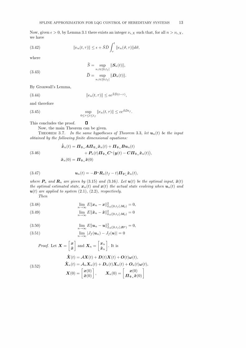
This concludes the proof.Now, the main Theorem can be given.Theorem 3.7. In the same hypotheses of Theorem 3.3, let un(t) be the input
obtained by the following ¯nite dimensional equations:
(3.46)
_xn(t) =¦ªnA¦ªnxn(t) +¦ªnBun(t)
+Pn(t)¦ªnC¤¡y(t)¡C¦ªnxn(t)¢;
xn(0) =¦ªnx(0)
(3.47) un(t) = ¡B¤Rn(tf ¡ t)¦ª0nxn(t);
where Pn and Rn are given by (3.15) and (3.16). Let u(t) be the optimal input, x(t)the optimal estimated state, xn(t) and x(t) the actual state evolving when un(t) andu(t) are applied to system (2.1), (2.2), respectively.
Then
limn!1Ekxn ¡ xk
2L2([0;tf ];M2)
= 0;(3:48)
limn!1Ekxn ¡ xk
2L2([0;tf ];M2)
= 0(3:49)
limn!1Ekun ¡ uk
2L2([0;tf ];IRp) = 0;(3:50)
limn!1 jJf (un)¡ Jf (u)j = 0(3:51)
Proof. Let X =
·xx
¸and Xn =
·xnxn
¸. It is
(3:52)
_X(t) = AX(t) +D(t)X(t) +O(t)!(t);_Xn(t) = AnXn(t) +Dn(t)Xn(t) +On(t)!(t);
X(0) =
·x(0)x(0)
¸; Xn(0) =
·x(0)
¦ªnx(0)
¸

14 ALFREDO GERMANI, COSTANZO MANES, AND PIERDOMENICO PEPE
where A;An;D(t);Dn(t);O(t);On(t) have been de¯ned in Lemma 3.5.
Let S(t), Sn(t), U(t; ¿), Un(t; ¿) as in Lemmas 3.5, 3.6. We have
X(t) = S(t)X(0) +
Z t
0
S(t¡ ¿)¡D(¿)X(¿) +O(¿)!(¿)¢d¿;(3:53)
Xn(t) = Sn(t)Xn(0) +
Z t
0
Sn(t¡ ¿)¡Dn(¿)Xn(¿) +On(¿)!(¿)
¢d¿;(3:54)
which can be rewritten as
X(t) = U(t; 0)X(0) +
Z t
0
U(t; ¿)O(¿)!(¿)d¿;(3.55)
Xn(t) = Un(t; 0)Xn(0) +
Z t
0
Un(t; ¿)On(¿)!(¿)d¿:(3.56)
Let us introduce the Hilbert spaces
(3:57) WX;t = L2([0; t];H); W!;t = L2([0; t]; IRs);
and de¯ne the operators
(3:58)
Lt :W!;t 7!WX;t;
f = Lt g; f(¿) =
Z ¿
0
U(¿; #)O(#)g(#)d#;
(3:59)
Lt;n :W!;t 7!WX;t
f = Lt;n g f(¿) =
Z ¿
0
Un(¿; #)On(#)g(#)d#;
and the functions
X0 : X0(¿) = U(¿; 0)X(0);(3:60)
X0;n : X0;n(¿) = Un(¿; 0)Xn(0);(3:61)
In the spaceWX;t equations (3.55) (3.56) can be expressed as
X =X0 +Lt!;(3:62)
Xn =X0;n +Lt;n!;(3:63)
so that
(3:64)EkX ¡Xnk2WX;t
= EkX0 ¡X0;n + (Lt ¡Lt;n)!k2WX;t
· 2EkX0 ¡X0;nk2WX;t+ 2Ek(Lt ¡Lt;n)!k2WX;t
:

SPLINE APPROXIMATION FOR LQG CONTROL OF HEREDITARY SYSTEMS 15
The ¯rst term in the right hand side goes to zero thanks to Lemma 3.6. For the secondterm we have
(3:65)
Ek(Lt ¡Lt;n)!k2W(X;t)
= kLt ¡Lt;nk2H:S:=
Z t
0
Z ¿
0
°°U(¿; #)O(#)¡Un(¿; #)On(#)°°2H:S:d#d¿· 2
Z t
0
Z ¿
0
°°°¡U(¿; #)¡Un(¿; #)¢O(#)°°°2H:S:
d#d¿
+ 2
Z t
0
Z ¿
0
°°°Un(¿; #)¡O(#)¡On(#)¢°°°2H:S:
d#d¿
· sup0·#·¿·t
supM2fO(#);#2[0;t]g
°°°¡U(¿; #)¡Un(¿; #)¢M°°°2H:S:
t2
+ sup0·#·¿·t; n2Z+
kUn(¿; #)kt2 sup#2[0;t]
kO(#)¡On(#)k2H:S:
which goes to zero by using Lemmas 3.1, 3.5 and 3.6. This concludes the proof.
4. The approximation scheme. In this section it will be derived the approxi-mation scheme for the LQG controller (3.4{3.7). The ¯rst step is the de¯nition of thesequences ªn and ª0n of subspaces approximating D(A) and D(A¤). This is made bya suitable de¯nition of basis vectors for subspaces ªn ½ D(A) and ª0n ½ D(A¤). Inorder to avoid confusion with general setting in section 3, the forthcoming choice forªn and ª0n will be denoted by ©n and ©0n respectively. In [3] the dynamics of lineardelay systems is approximated using classical ¯rst order splines uniformly distributedover the interval [¡r; 0]. With this choice the computation of matrix representationof the approximated operators is quite complex due to the fact that in general, for agiven number n of subintervals of [¡r; 0], the delay instants ¡rj do not coincide withknots of splines.
It is useful to de¯ne a multi-index s = (n1; : : : ; n±) that characterizes the partitionof each interval [¡ri;¡ri¡1], for i = 1; : : : ; ±, into ni subintervals of length (ri ¡ri¡1)=ni, in which ni + 1 classical ¯rst order splines are considered (see Figure 1),numbered from 0 to ni.
Definition 4.1. A sequence fsng of multi-indexes, de¯ned for n = 1; 2; : : :,where n is the lowest of indexes nj of the multi-index (i.e. n = minfsng), is denoteda test sequence if there exists a constant ¹c such that for each n it is maxfsng=n · ¹c.
Let tij = ¡ri¡1 ¡ (ri ¡ ri¡1)j=ni, for j = 0; 1; : : : ; ni, i = 1; : : : ; ±. Let splineij bethe spline j of interval i, that is the spline with knot in tij . Let Ák, k = 1; 2; : : : ; N; be
the canonical base in IRN .The approximating subspace ©n and ©0n are de¯ned as follows:Definition 4.2. For any given multi-index sn of a test sequence let ©n be the
subspace of linear combinations of vectors vih, vrik de¯ned as follows:
(4:1) v1k =
·Ák
Ákspline10
¸; k = 1; : : : ; N:
(4:2) vijN+k =
·0
Áksplineij
¸; k = 1; : : : ; N; j = 1; : : : ; ni ¡ 1:

16 ALFREDO GERMANI, COSTANZO MANES, AND PIERDOMENICO PEPE
Fig. 1. First order splines used for the approximation schemes
(4:3) v±n±N+k =
·0
Ákspline±n±
¸; k = 1; : : : ; N:
(4:4) vrik =
·0
Áksplineri
¸;
i = 1; : : : ; ± ¡ 1;k = 1; : : : ;N:
where
(4:5) splineri = splineini ¢ Â(¡ri;¡ri¡1] + splinei+10 ; i = 1; : : : ; ± ¡ 1:
Definition 4.3. For any given multi-index sn of a test sequence let ©0n be thesubspace of linear combinations of vectors wih, w
rik , w
0k de¯ned as follows:
w1k =
·0
Ákspline10
¸; k = 1; : : : ;N;(4.6)
wijN+k = vijN+k k = 1; : : : ;N;
i = 1; : : : ; ±;
j = 1; : : : ; ni ¡ 1;(4.7)
(4.8) wrjk =
·0
Ákspline0rj
¸; j = 1; : : : ; ± ¡ 1; k = 1; : : : ; N:
where
spline0rj =(± ¡ j)
(± ¡ j + 1)splinejnj ¢ Â(¡rj ;¡rj¡1] + splinej+10 ;(4:9)
spline00rj = splinejnj ¢ Â(¡rj ;¡rj¡1]; j = 1; : : : ; ± ¡ 1;(4:10)

SPLINE APPROXIMATION FOR LQG CONTROL OF HEREDITARY SYSTEMS 17
(4.11) w0k =·
Áka±kspline
±n± +
P±¡1j=1
1(±¡j+1)ajkspline
00rj
¸; k = 1; : : : ;N;
where ajk is the k column of matrix ATj , for j = 1; : : : ; ±.
Theorem 4.4. For each multi-index sn of a test sequence, it is ©n ½ D(A) and©0n ½ D(A¤).
Proof. It is immediate to verify that ©n ½ D(A). A more detailed proof isrequired to show that ©0n ½ D(A¤). To this aim is su±cient to verify that each vectorw belongs to it. It is easy to check that vectors wijN+k, for i = 1; : : : ; ±, k = 1; : : : ; N ,
j = 1; : : : ; ni ¡ 1 and vectors w1k, for k = 1; : : : ; N , belong to D(A¤). Let us considernow the vectors wrik , for i = 1; : : : ; ±¡ 1, k = 1; : : : ; N (as usual, we shall indicate the
part in IRN by using the subscript 0, and the part in L2 by using the subscript 1).From de¯nition, for each k it is
(4:12)
(wrik )0 = 0;
(wrik )1 (¡rj) = 0; i; j = 1; : : : ; ± ¡ 1; i6= j;(wrik )1 (¡r) = 0; i = 1; : : : ; ± ¡ 1;
so that for k = 1; : : : ; N; i = 1; : : : ; ± ¡ 1
(4:13) (wrik )1 (¡r) = AT± (w
rik )0
and
(4:14)
±¡1Xj=1
kj ((wrik )0; (w
rik )1)Â[¡r;¡rj ] =
±¡1Xj=1
(wrik )1 (¡rj)¡ATj (w
rik )0
± ¡ j + 1 Â[¡r;¡rj ]
=(wrik )1 (¡ri)± ¡ i+ 1 Â[¡r;¡ri]:
So it is only to be veri¯ed that for i = 1; : : : ; ± ¡ 1; k = 1; : : : ;N :
(4.15) (wrik )1 ¡1
(± ¡ i+ 1) (wrik )1 (¡ri)Â[¡r;¡ri] 2W 1;2:
Since
(4:16) spline0ri(¡ri)¡1
± ¡ i+ 1 =± ¡ i
± ¡ i+ 1 = lim#!¡r+
i
spline0ri(#);
(4.15) is clearly true.For vectors w0k de¯ned in (4.11), for k = 1; : : : ; N it is
(4.17) (w0k)1(¡r) = a±k = AT± Ák = A
T± (w
0k)0:
It is also
(4:18) (w0k)1(¡ri) = 0; i = 1; : : : ; ± ¡ 1;

18 ALFREDO GERMANI, COSTANZO MANES, AND PIERDOMENICO PEPE
and therefore
(4:19)
±¡1Xj=1
kj ((w0k)0; (w0k)1)Â[¡r;¡rj ] =
±¡1Xj=1
(w0k)1 (¡rj)¡ATj (w
0k)0
± ¡ j + 1 Â[¡r;¡rj ]
=±¡1Xj=1
¡ATj (w
0k)0
(± ¡ j + 1) Â[¡r;¡rj ] =±¡1Xj=1
¡ajk(± ¡ j + 1)Â[¡r;¡rj ]:
From
(4:20) lim#7!¡r+
j
(w0k)1 (#) =ajk
± ¡ j + 1
it follows, for i = 1; : : : ; ± ¡ 1
(4:21)
³(w0k)1+
±¡1Xj=1
ajk(± ¡ j + 1)Â[¡r;¡rj ]
´(¡ri) = (w0k)1(¡ri) +
iXj=1
ajk(± ¡ j + 1)
=iX
j=1
ajk± ¡ j + 1 =
aik± ¡ i+ 1 +
i¡1Xj=1
ajk± ¡ j + 1
= lim#7!¡r+
i
(w0k)1 (#) + lim#7!¡r+
i
±¡1Xj=1
ajk± ¡ j + 1Â[¡r;¡rj ](#);
and so
(4.22)³(w0k)1 +
±¡1Xj=1
ajk± ¡ j + 1Â[¡r;¡rj ]
´2W 1;2
(4.17) and (4.22) prove that vectors w0k, k = 1; : : : ; N , belong to D(A¤).Remark 4.5. Note that a key idea for the previous theorem is the choice of a
type of not uniformly distributed splines.Remark 4.6. In the case of just one pure delay, vectors generating subspaces
©n and ©0n become, respectively,
(4:23) vjN+k =
·0
Áksplinej
¸; k = 1; : : : ; N; j = 1; 2; : : : ; n
(4:24) vk =
·Ák
Ákspline0
¸; k = 1; : : : ; N
for ©n, and
(4:25) w1k =
·0
Ákspline0
¸; k = 1; : : : ; N;
(4:26) wjN+k = vjN+k k = 1; : : : ;N; j = 1; 2; : : : ; n¡ 1
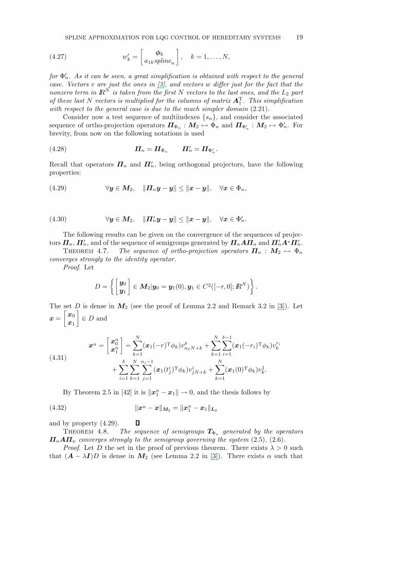
SPLINE APPROXIMATION FOR LQG CONTROL OF HEREDITARY SYSTEMS 19
(4:27) w0k =·
Áka1ksplinen
¸; k = 1; : : : ; N;
for ©0n. As it can be seen, a great simpli¯cation is obtained with respect to the generalcase. Vectors v are just the ones in [3], and vectors w di®er just for the fact that thenonzero term in IRN is taken from the ¯rst N vectors to the last ones, and the L2 partof these last N vectors is multiplied for the columns of matrix AT
1 . This simpli¯cationwith respect to the general case is due to the much simpler domain (2.21).
Consider now a test sequence of multiindexes fsng, and consider the associatedsequence of ortho-projection operators ¦©n :M2 7! ©n and ¦©0n : M2 7! ©0n. Forbrevity, from now on the following notations is used
(4:28) ¦n =¦©n ¦ 0n =¦©0n :
Recall that operators ¦n and ¦ 0n, being orthogonal projectors, have the following
properties:
(4.29) 8y 2M2; k¦ny ¡ yk · kx¡ yk; 8x 2 ©n;
(4.30) 8y 2M2; k¦ 0ny ¡ yk · kx¡ yk; 8x 2 ©0n:
The following results can be given on the convergence of the sequences of projec-tors¦n,¦ 0
n, and of the sequence of semigroups generated by¦nA¦n and¦ 0nA¤¦ 0
n.Theorem 4.7. The sequence of ortho-projection operators ¦n : M2 7! ©n
converges strongly to the identity operator.Proof. Let
D =
½·y0y1
¸2M2jy0 = y1(0);y1 2 C2([¡r; 0]; IRN )
¾:
The set D is dense in M2 (see the proof of Lemma 2:2 and Remark 3:2 in [3]). Let
x =
·x0x1
¸2 D and
(4:31)
xn =
·xn0xn1
¸=
NXk=1
(x1(¡r)TÁk)v±n±N+k +NXk=1
±¡1Xi=1
(x1(¡ri)TÁk)vrik
+±Xi=1
NXk=1
ni¡1Xj=1
(x1(tij)TÁk)vijN+k +
NXk=1
(x1(0)TÁk)v1k:
By Theorem 2.5 in [42] it is kxn1 ¡ x1k ! 0; and the thesis follows by
(4:32) kxn ¡ xkM2 = kxn1 ¡ x1kL2and by property (4.29).
Theorem 4.8. The sequence of semigroups T©n generated by the operators¦nA¦n converges strongly to the semigroup governing the system (2.5), (2.6).
Proof. Let D the set in the proof of previous theorem. There exists ¸ > 0 suchthat (A ¡ ¸I)D is dense in M2 (see Lemma 2.2 in [3]). There exists ® such that

20 ALFREDO GERMANI, COSTANZO MANES, AND PIERDOMENICO PEPE
(A¡®I) e (¦nA¦n¡®I) are dissipative (see Lemma 2.3 and proof of Theorem 3.1
in [3]). Let x =
·x0x1
¸2 D. Let ¦nx =
·(¦nx)0(¦nx)1
¸. From
(4:33) (¦nx)1(¡ri) = (¦nx)1(¡ri¡1)¡Z ¡ri¡1
¡ri
d(¦nx)1(#)
d#d#
and as kd(x1¡(¦nx)1)d# k ! 0, (see theorem 4.1 in [3], and theorems 1.5, 2.5 in [42]),
it follows that kA¦nx ¡ Axk ! 0. For, just take into account that (¦nx)1(0) =(¦nx)0, and that k(¦nx)0 ¡ x0k ! 0. It follows that the Trotter-Kato theoremhypotheses are satis¯ed ([38], Lemma 3.1 in [3]).
As it can be seen the proofs of the above two theorems follow the same lines ofthe proofs in [3], developed for the case of ¯rst order splines uniformly distributed inthe interval [¡r; 0].
Lemma 4.9. The subspace
(4.34) U =
(·y0y1
¸ ¯ y0 2 IRN ;y1 2W 1;2
y1(0) = y0;
y1(¡rj) = ATj y0; j = 1; : : : ; ±
);
is dense in M2.
Proof. As usual, let us prove density in IRN £W 1;2. Let y =
·y0y1
¸2 IRN £
W 1;2. Let us de¯ne the following sequence of functions fn : [¡r; 0] ! IRN , n >supi=1;2;:::;±
rri¡ri¡1 ,
(4:35)
fn(#) =
µy0 ¡ n
r#(y1(
¡rn)¡ y0)
¶Â[¡rn ;0]+³
AT± y0 +
n
r(#+ r)(y1(¡r + r
n)¡AT
± y0´Â[¡r;¡r+ r
n ]
+±Xi=1
³ATi y0 +
n
r(#+ ri)(y1(¡ri + r
n)¡AT
i y0)´Â[¡ri;¡ri+ r
n ]+
+³ATi y0 ¡
n
r(#+ ri)(y1(¡ri ¡ r
n)¡AT
i y0)´Â[¡ri¡ r
n ;¡ri)
Consider the sequence of elements in U ,
(4:36) yn =
·y0
fn +P±
i=1 y1Â(¡ri+ rn ;¡ri¡1¡ r
n )
¸As y1 is bounded, fn is bounded too, uniformly on n. It follows
(4:37) kyn ¡ yk2 ·Ãsup#;n
ky1(#)¡ fn(#)k2!2±r
n:
Remark 4.10. The previous Lemma proves that the intersection between thedomain of A and the domain of A¤ is dense in M2, if the weighted inner productis used. For, just see that the subspace U is contained in both the domains. It is astandard result that such an intersection is in general not dense, if the usual innerproduct is used [11,14,24,27,43].

SPLINE APPROXIMATION FOR LQG CONTROL OF HEREDITARY SYSTEMS 21
Theorem 4.11. The sequence of ortho-projection operators ¦ 0n : M2 7! ©0n
converges strongly to the identity operator.
Proof. It is su±cient to prove strong convergence in a dense subspace of M2.Therefore, consider the subspace U in (4.34).
It is shown below that for any y =
·y0y1
¸2 U there exists a sequence of approxi-
mations yn 2 ©0n such that limn!1 kyn¡ykM2 = 0. Consider the following de¯nitionof yn 2 ©0n
(4:38)
yn =NXk=1
(yT0 Ák)w0k +
NXk=1
±¡1Xi=1
(y1(¡ri)TÁk)wrik
+±Xi=1
NXk=1
ni¡1Xj=1
(y1(tij)TÁk)wijN+k +
NXk=1
(y1(0)TÁk)w1k:
It is, by substituting expressions (4.6),(4.7), (4.8), (4.11), of vectors generating thesubspace ©0n
(4:39)
yn =
·yn0yn1
¸=
·y0PN
k=1(y1(¡r)TÁk)Ákspline±n±
¸+
"0PN
k=1
P±¡1j=1
µ(yT0 Ák)ajk± ¡ j + 1 spline
00rj + (y1(¡rj)TÁk)Ákspline0rj
¶#
+
·0P±
i=1
PNk=1
Pni¡1j=1 (y1(t
ij)TÁk)Ákspline
ij
¸+
·0PN
k=1(y1(0)TÁk)Ákspline
10
¸:
Moreover it is readily recognized that
(4:40)NXk=1
(yT0 Ák)aAK = ATj y0 =
NXk=1
(y1(¡rj)TÁk)Ák; j = 1; : : : ; ±;
(4:41)1
± ¡ j + 1spline00rj + spline
0rj = splinerj ; j = 1; : : : ; ± ¡ 1;

22 ALFREDO GERMANI, COSTANZO MANES, AND PIERDOMENICO PEPE
so that
(4:42)
kyn ¡ ykM2
=°°° NXk=1
(y1(¡r)TÁk)Ákspline±n± +±¡1Xj=1
ATj y0
³ 1
± ¡ j + 1spline00rj + spline
0rj
´
+±Xi=1
NXk=1
ni¡1Xj=1
(y1(tij)TÁk)Ákspline
ij +
NXk=1
(y1(0)TÁk)Ákspline10 ¡ y1
°°°L2
=°°° NXk=1
(y1(¡r)TÁk)Ákspline±n± +±¡1Xj=1
y1(¡rj)splinerj
+±Xi=1
NXk=1
ni¡1Xj=1
(y1(tij)TÁk)Ákspline
ij +
NXk=1
(y1(0)TÁk)Ákspline10 ¡ y1
°°°L2
=°°° ±Xi=1
NXk=1
niXj=0
(y1(tij)TÁk)Ákspline
ij ¡ y1
°°°L2
=±Xi=1
°°° NXk=1
niXj=0
(y1(tij)TÁk)Ákspline
ij ¡ y1 ¢ Â[¡ri;¡ri¡1]
°°°L2
which gives the norm of the error between a function y1 2W 1;2 and its approximationwith ¯rst order splines in which the value at each spline knot (the instants tij) is exactly
the value of the function at time tij . It is a standard result that the error tends to zeroin L2 norm for n ! 1 (theorem 2.4 in [42]) and therefore limn!1 kyn ¡ ykM2 = 0.This implies, by property (4.30), the strong convergence to identity of operator ¦ 0
n.
Lemma 4.12. There exists a real constant ® such that the operator A¤¡®I andoperators ¦ 0
nA¤¦ 0n ¡ ®I are dissipative
Proof. In [3] it has been proved that there exists ® such that operator A ¡®I is dissipative, and therefore generates a semigroup which is a contraction one.This implies that the adjoint semigroup is a contraction one too, and therefore itsin¯nitesimal generator A¤ ¡ ®I is dissipative [1]. Dissipativity of A¤ ¡ ®I impliesthat for any n the operator ¦ 0
nA¤¦ 0n ¡ ®I is dissipative. This happens because for
any x 2M2
(4:43)
((¦ 0nA¤¦ 0
n ¡ ®I)x;x) = (A¤¦ 0nx;¦ 0
nx)¡ ®(x;x)· (A¤¦ 0
nx;¦ 0nx)¡ ®(¦ 0
nx;¦ 0nx)
= ((A¤ ¡ ®I)¦ 0nx;¦ 0
nx) · 0:
Lemma 4.13. Let D be the dense subspace of M2 de¯ned as
(4:44) D =
8>><>>:24y0y1
35 ¯ y0 2 IRN ; AT± y0 = y1(¡r);³
y1 ¡±¡1Xj=1
kj(y0;y1)Â[¡r;¡rj ]´2 C2
9>>=>>;Then, there exists ¸ > 0 such that (A¤ ¡ ¸I)D is dense in M2.
SPLINE APPROXIMATION FOR LQG CONTROL OF HEREDITARY SYSTEMS 23
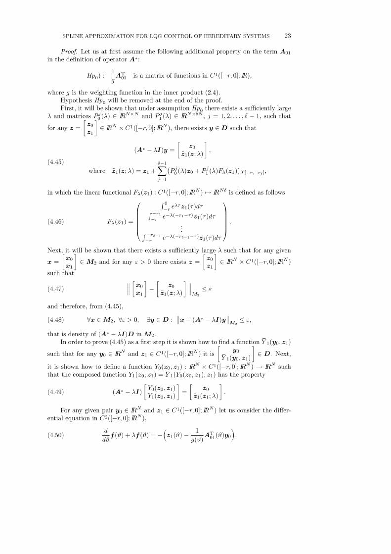
Proof. Let us at ¯rst assume the following additional property on the term A01
in the de¯nition of operator A¤:
Hp0) :1
gAT01 is a matrix of functions in C1([¡r; 0]; IR),
where g is the weighting function in the inner product (2.4).Hypothesis Hp0 will be removed at the end of the proof.First, it will be shown that under assumption Hp0 there exists a su±ciently large
¸ and matrices P j0 (¸) 2 IRN£N and P j1 (¸) 2 IRN£±N , j = 1; 2; : : : ; ± ¡ 1, such thatfor any z =
·z0z1
¸2 IRN £ C1([¡r; 0]; IRN ), there exists y 2D such that
(4.45)
(A¤ ¡ ¸I)y =·
z0~z1(z;¸)
¸;
where ~z1(z;¸) = z1 +±¡1Xj=1
¡P j0 (¸)z0 + P
j1 (¸)F¸(z1)
¢Â[¡r;¡rj ];
in which the linear functional F¸(z1) : C1([¡r; 0]; IRN )7! IRN± is de¯ned as follows
(4.46) F¸(z1) =
0BBBB@R 0¡r e
¸¿z1(¿)d¿R¡r1¡r e¡¸(¡r1¡¿)z1(¿)d¿
...R ¡r±¡1¡r e¡¸(¡r±¡1¡¿)z1(¿)d¿
1CCCCA :Next, it will be shown that there exists a su±ciently large ¸ such that for any given
x =
·x0x1
¸2M2 and for any " > 0 there exists z =
·z0z1
¸2 IRN £ C1([¡r; 0]; IRN )
such that
(4:47)°°° ·x0x1
¸¡·
z0~z1(z;¸)
¸ °°°M2
· "
and therefore, from (4.45),
(4:48) 8x 2M2; 8" > 0; 9y 2D :°°x¡ (A¤ ¡ ¸I)y°°
M2· ";
that is density of (A¤ ¡ ¸I)D inM2.In order to prove (4.45) as a ¯rst step it is shown how to ¯nd a function Y 1(y0;z1)
such that for any y0 2 IRN and z1 2 C1([¡r; 0]; IRN ) it is·
y0Y 1(y0;z1)
¸2 D. Next,
it is shown how to de¯ne a function Y0(z0;z1) : IRN £ C1([¡r; 0]; IRN ) ! IRN such
that the composed function Y1(z0;z1) = Y 1(Y0(z0;z1);z1) has the property
(4:49) (A¤ ¡ ¸I)·Y0(z0;z1)Y1(z0;z1)
¸=
·z0
~z1(z1;¸)
¸:
For any given pair y0 2 IRN and z1 2 C1([¡r; 0]; IRN ) let us consider the di®er-ential equation in C2([¡r; 0]; IRN ),
(4.50)d
d#f(#) + ¸f(#) = ¡
³z1(#)¡ 1
g(#)AT01(#)y0
´;

24 ALFREDO GERMANI, COSTANZO MANES, AND PIERDOMENICO PEPE
whose solution is
(4.51) f(#) = e¡¸(#+r)f(¡r)¡Z #
¡re¡¸(#¡¿)
³z1(¿)¡ 1
g(¿)AT01(¿)y0
´d¿:
By Lemma A.1 in Appendix, there exists a unique left-continuous function y1 thatsatis¯es condition (A.1), with f given by (4.51). Such y1 is given by expression (A.6),and its values at the delay instants are such that
(4.52) (I(±¡1)N ¡H±;2)
264 y1(¡r1)...
y1(¡r±¡1)
375 =264 f(¡r1)
...f(¡r±¡1)
375¡H±;2264 AT
1...
AT±¡1
375y0where H±;2 is de¯ned in (A.4), Lemma A.1, in appendix.
In order to guarantee that y =
·y0y1
¸2D, y1 must satisfy the additional condi-
tion
(4.53) y1(¡r) = AT± y0;
By substituting (4.53) in (A.1) one has
(4.54) f(¡r) = AT± y0 ¡
±¡1Xj=1
y1(¡rj)¡ATj y0
± ¡ j + 1 ;
that can be rewritten as
(4.55) f(¡r) = h±;1
264 y1(¡r1)...
y1(¡r±¡1)
375¡ h±;2264 AT
1...
AT±¡1
375y0;where
(4.56)h±;1 = [
1±IN ¢ ¢ ¢ 1
2IN IN ] ;
h±;2 = [1±IN ¢ ¢ ¢ 1
2IN ] :
By (4.51) the values of function f at the delay instants are as follows
(4.57)
264 f(¡r1)...
f(¡r±¡1)
375 =24 INe¡¸(r¡r1)
...INe¡¸(r¡r±¡1)
35f(¡r)¡ £0(±¡1)N£N I(±¡1)N
¤F¸¡z1 ¡ 1
gAT01y0
¢:
By substituting (4.52) and (4.55) into (4.57) and rearranging we have
(4.58)
Hp(¸)
264 y1(¡r1)...
y1(¡r±¡1)
375 = Hq(¸)264 AT
1...
AT±¡1
375y0¡ £0(±¡1)N£N I(±¡1)N
¤ ³F¸(z1)¡ F¸
¡1gAT01
¢y0´;
SPLINE APPROXIMATION FOR LQG CONTROL OF HEREDITARY SYSTEMS 25
in which matrices Hp and Hq are de¯ned as
Hp(¸) = I(±¡1)N ¡H±;2 +24 INe¡¸(r¡r1)
...INe¡¸(r¡r±¡1)
35h±;2;(4.59)
Hq(¸) =
24 INe¡¸(r¡r1)...
INe¡¸(r¡r±¡1)
35h±;1 ¡ · H±;20N£±N
¸:(4:60)
Because Hp is nonsingular (Lemma A.3 in Appendix), by (4.58) it results
(4:61)
264 y1(¡r1)...
y1(¡r±¡1)
375 = ¡ £0(±¡1)N£N H¡1p (¸)
¤F¸(z1)
+³H¡1p (¸)Hq(¸)
264 AT1...
AT±¡1
375+ £0(±¡1)N£N H¡1p (¸)
¤F¸¡1gAT01
¢´y0:
From (4.61) and (4.53), recalling that r± = r, matrices Nj(¸) and Mj(¸), j = 1; : : : ; ±are de¯ned such that
(4.62) y1(¡rj) = Nj(¸)y0 +Mj(¸)F¸(z1):
The left-continuous function y1 = Y 1(y0;z1) we were looking for is given by
(4.63) y1(#) =
8><>:y1(¡ri); # = ¡ri,
f(#) +±¡1Xj=1
y1(¡rj)¡ATj y0
± ¡ j + 1 Â[¡r;¡rj ](#) #6= ¡ri;
where i = 1; : : : ; ±¡ 1, and in which f(#) is given by (4.51). With this de¯nition it isy =
·y0y1
¸2D. Let
(A¤ ¡ ¸I)y =·[(A¤ ¡ ¸I)y]0[(A¤ ¡ ¸I)y]1
¸:
It is
(4:64)
[(A¤ ¡ ¸I)y]1
=1
gAT01y0 ¡
d
d#
0@y1 ¡ ±¡1Xj=1
y1(¡rj)¡ATj y0
± ¡ j + 1 Â[¡r;¡rj ]
1A¡ ¸y1=1
gAT01y0 ¡
d
d#f ¡ ¸f ¡ ¸
±¡1Xj=1
y1(¡rj)¡ATj y0
± ¡ j + 1 Â[¡r;¡rj ]:
Finally, recalling the de¯nition (4.50) of function f it is
(4.65) [(A¤ ¡ ¸I)y]1 = z1 ¡ ¸±¡1Xj=1
¡Nj(¸)¡AT
j
¢y0 +Mj(¸)F¸(z1)
± ¡ j + 1 Â[¡r;¡rj ]:
26 ALFREDO GERMANI, COSTANZO MANES, AND PIERDOMENICO PEPE
Until now we have showed that, for any y0 2 IRN and for any z1 2 C1([¡r; 0]; IRN ) itis possible to ¯nd y1 such that y =
·y0y1
¸2D and satis¯es (4.65).
Now, using the computed y1 = Y 1(y0;z1), we are ready to prove that there existsa positive ¸ such that for any z0 2 IRN and z1 2 C1([¡r; 0]; IRN ), a y0 can be foundsuch that y =
·y0y1
¸2D and satis¯es (4.45). The application of operator (A¤ ¡ ¸I)
gives, for the part in IRN ,
(4:66) [(A¤ ¡ ¸I)y]0 = ± y1(0) +AT0 y0 ¡ ¸y0:
Note that from (4.63) y1(0) = f(0) and evaluation of f(0) according to equation(4.51), in which expression (4.54) of f(¡r) is substituted, gives
(4.67) [(A¤ ¡ ¸I)y]0 = Q0(¸)y0 +Q1(¸)F¸(z1);
in which
(4.68)
Q0(¸) = ±e¡¸rAT± ¡ ±e¡¸r
±¡1Xj=1
Nj(¸)¡ATj
(± ¡ j + 1)
+ ±
Z 0
¡re¸¿
1
gAT01d¿ +A
T0 ¡ ¸IN ;
Q1(¸) = ¡± [ IN£N 0N£N(±¡1) ]¡±¡1Xj=1
±e¡¸r
± ¡ j + 1Mj(¸):
It is clear that there exists a su±ciently large ¸ such that Q0(¸) is nonsingular, dueto the presence of the term ¡¸IN (the other terms are all bounded functions of ¸).Therefore, given z0 2 IRN and z1 2 C1([¡r; 0]; IRN ), the function Y0(z0;z1) = y0 2IRN such that [(A¤ ¡ ¸I)y]0 = z0, thanks to eq. (4.67), is given by
(4.69) y0 = Y0(z0;z1) = Q¡10 (¸)
³z0 ¡Q1(¸)F¸(z1)
´:
Substitution of (4.69) in the expression (4.65) for [(A¤ ¡ ¸I)y]1 gives
(4:70)
[(A¤ ¡ ¸I)y]1 = z1 ¡ ¸±¡1Xj=1
¡Nj(¸)¡AT
j
¢Q¡10 (¸)z0
(± ¡ j + 1) Â[¡r;¡rj ]¡
¡ ¸±¡1Xj=1
¡Nj(¸)¡AT
j
¢Q¡10 (¸)Q1(¸)F¸(z1) +Mj(¸)F¸(z1)
(± ¡ j + 1) Â[¡r;¡rj ]:
This expression allows to de¯ne the matrices P j0 (¸) and Pj1 (¸) used in (4.45) as
(4:71)
P j0 = ¡¸¡Nj(¸)¡AT
j
¢Q¡10 (¸)
(± ¡ j + 1) ;
P j1 = ¡¸¡Nj(¸)¡AT
j
¢Q¡10 (¸)Q1(¸) +Mj(¸)
(± ¡ j + 1) :

SPLINE APPROXIMATION FOR LQG CONTROL OF HEREDITARY SYSTEMS 27
Composition of functions Y 1(y0;z1) and Y0(z0;z1) gives the announced function
Y1(z0;z1). This concludes the proof that, for ¸ su±ciently large, for any
·z0z1
¸2
IRN £ C1([¡r; 0]; IRN ) there exists·y0y1
¸2D such that (4.45) holds.
Consider now the continuous linear function ©¸ de¯ned as follows
(4:72)
©(¸) : L2([¡r; 0]; IRN)7! L2([¡r; 0]; IRN );
©(¸)(g) = g +±¡1Xj=1
P j1 (¸)F¸(g)Â[¡r;¡rj ]:
Let us de¯ne the following subspace of L2([¡r; 0]; IRN)
(4:73) R = ©(¸)¡C1([¡r; 0]; IRN)¢:The proof of 2) is obtained if the set R is proved to be dense in L2([¡r; 0]; IRN ). Thisis true because it can be readily shown that density of R is su±cient to conclude that8x 2 M2, for any " > 0, there exists a y 2 D such that kx ¡ (A¤ ¡ ¸I)ykM2 · "(i.e., density of (A¤ ¡ ¸I)D).
Given a x =
·x0x1
¸2M2, take yA 2D as follows: yA;0 = Y0(x0; 0) = Q
¡10 (¸)x0
and yA;1 = Y1(x0; 0). It is, by construction
(4:74) (A¤ ¡ ¸I)yA =·
x0P±¡1j=1 P
j0 (¸)x0Â[¡r;¡rj ]
¸:
From density of R, there exists zB;1 2 C1([¡r; 0]; IRN ) such that the function
(4:75) ~zB;1 = zB;1 +±¡1Xj=1
P j1 (¸)F¸(zB;1)Â[¡r;¡rj ]
satis¯es
(4:76)°°° ±¡1Xj=1
P j0 (¸)x0Â[¡r;¡rj ] ¡ ~zB;1°°°L2· "
2;
and from result (4.45) there exists yB 2D such that (A¤ ¡ ¸I)yB =·0~zB;1
¸.
Exploiting again density of R there exists zC;1 2 C1([¡r; 0]; IRN ) such that thefunction
(4:77) ~zC;1 = zC;1 +±¡1Xj=1
P j1 (¸)F¸(zC;1)Â[¡r;¡rj ]
satis¯es
(4:78)°°°x1 ¡ ~zC;1°°°
L2· "
2:

28 ALFREDO GERMANI, COSTANZO MANES, AND PIERDOMENICO PEPE
Again, from result (4.45) there exists yC 2D such that (A¤¡¸I)yC =·0~zC;1
¸. It is
now an easy matter to show that vector y = yA ¡ yB + yC is such that
(4:79)
kx¡ (A¤ ¡ ¸I)ykM2 = kx¡ (A¤ ¡ ¸I)(yA ¡ yB + yC)kM2
·°°° · 0x1 ¡ [(A¤ ¡ ¸I)yA]1 + ~zB;1 ¡ ~zC;1
¸°°°M2
· °°x1 ¡ ~zC;1°°L2 + °°° ±¡1Xj=1
P j0 (¸)x0Â[¡r;¡rj ] ¡ ~zB;1°°°L2· ":
It remains to prove that R is dense for su±ciently large ¸. We will show that if forany f 2 L2([¡r; 0]; IRN ) there exists a vector ® 2 IRN± such that
(4.80) F¸(f)¡ F¸³±¡1Xj=1
P j1®Â[¡r;¡rj ]´¡ ® = 0
then for any f 2 L2([¡r; 0]; IRN) a sequence ffkg, fk 2 R 8k ¸ 0, can be found suchthat kf ¡ fkkL2 ! 0. Existence of ® in (4.80) for any f is ensured by nonsingularityof matrix
(4.81) ¡(¸) = IN±£N± +±¡1Xj=1
F¸¡P j1 (¸)Â[¡r;¡rj ]
¢;
for su±ciently large ¸, that therefore is a su±cient condition for density of R.To this purpose consider a f 2 L2, let ® be the solution of (4.80) and de¯ne the
function
(4:82) f = f ¡±¡1Xj=1
P j1®Â[¡r;¡rj ];
It is such that ©(¸)(f) = f . Let fgkg be a sequence of functions in C1([¡r; 0]; IRN )such that kf ¡ gkkL2 ! 0. From continuity of function ©(¸) it is k©(¸)(f) ¡©(¸)(gk)kL2 ! 0. De¯ning functions fk = ©(¸)(gk) 2 R, the sequence ffkg con-verges to ©(¸)(f), that is f , and density of R, under nonsingularity of ¡(¸), is proved.
It remains to prove nonsingularity of the ±N £ ±N matrix ¡(¸) de¯ned in (4.81)for a su±ciently large ¸. Such proof is reported in [39], and is worked out by showingthat det
¡¡(¸)
¢is a continuous function of ¸ and that there exists the limit matrix
¡ = lim¸!+1 ¡(¸). Such matrix can be easily proved to be nonsingular, because it isblock triangular (each block is N £N), in which the diagonal consists of the followingnonsingular ± blocks: block 1 is IN , block j, for j = 2; : : : ; ±, is I + 1
±¡j+1IN . Itfollows that lim¸!+1 det
¡¡(¸)
¢= det
¡¡¢6= 0, and therefore there exists ¸0 such that
for every ¸ > ¸0 matrix ¡(¸) is nonsingular.So, chosen ¸ such that ¡(¸) and Q0(¸) are both nonsingular, the proof of propo-
sition 2) is completed in the case of hypothesis Hp0.To remove such hypothesis it is su±cient to consider a sequence Ak
01 in the spaceL2([¡r; 0]; IRN£N ), which converges to A01 and satis¯es hypothesis Hp0. For, let A
¤k
be the corresponding sequence of operators. Let Dk 2 L(M2) be de¯ned as
Dk
·y0y1
¸=
·0
1g (A
k01 ¡A01)Ty0
¸

SPLINE APPROXIMATION FOR LQG CONTROL OF HEREDITARY SYSTEMS 29
So A¤k = A
¤ +Dk and kDkkL(M2) · kAk01 ¡A01kL2([¡r;0];IRN£N) . From Proposition
2.3 in [5], page 28, and Theorem 1:1 in [38], page 76, it follows that any ¸ withRe(¸) > !0+supk kDkk belongs to the resolvent set of A¤ and A¤
k, for every k, where!0 is such that kT (t)k · e!0t, T (t) being the semigroup generated by A (see Lemma2.3 in [3]). Let us choose a ¸ in the resolvent sets ofA¤ and A¤
k, such that (A¤k¡¸I)D
is dense inM2, for every k. For, it is su±cient that corresponding matrices ¡k(¸) in(4.81) and Qk0(¸) in (4.68) are nonsingular. So, given x 2M2, given ² > 0, a sequenceyk can be found such that
(4.83) k(A¤k ¡ ¸I)yk ¡ xk <
²
2:
From
(4:84) k(A¤ ¡ ¸I)yk ¡ xk · k(A¤k ¡ ¸I)yk ¡ xk+ kDkkkykk;
it follows that there exist k0 such that k(A¤¡¸I)yk0¡xk < ², provided yk is uniformlybounded. For, it is su±cient that kDk0k < ²
2 supk kykk : It remains to prove uniformboundedness of yk. Let vk = (A¤
k ¡ ¸I)yk ¡ x. From (4.83) it is kvkk < ²2 for every
k. From
(4:85) (A¤k ¡ ¸I)¡1 =(A¤ +Dk ¡ ¸I)¡1 = [I ¡ (¸I ¡A¤)¡1Dk]¡1(A¤ ¡ ¸I)¡1
it follows
(4:86) k(A¤k ¡ ¸I)¡1k · k[I ¡ (¸I ¡A¤)¡1Dk]¡1kk(A¤ ¡ ¸I)¡1k
If k is su±ciently large such that k(¸I ¡A¤)¡1Dkk · d < 1, the following inequalityholds
(4:87) k[I ¡ (¸I ¡A¤)¡1Dk]¡1k ·1Xl=0
k(¸I ¡A¤)¡1Dkkl · 1
1¡ d
which proves the uniform boundedness of k(A¤k ¡ ¸I)¡1k. The uniform boundedness
of yk follows by
(4:88) yk = (A¤k ¡ ¸I)¡1(vk ¡ x):
Such a device to prove density of (A¤ ¡ ¸I)D in M2 when hypothesis Hp0 is notsatis¯ed has been introduced in [24], Theorem 7.2, for the one delay case.
Lemma 4.14. The operator ¦ 0nA¤¦ 0
n converges strongly to the operator A¤ inthe subspace D de¯ned in Lemma 4.13.
Proof. Since it is
(4:89) k¦ 0nA¤¦ 0
nx¡A¤xkM2 · k¦ 0n(A¤¦ 0
n ¡A¤)xkM2 + k¦ 0nA¤x¡A¤xkM2 ;
and limn!1 k¦ 0ny¡ykM2 = 0, 8y 2M2 (strong convergence), the Lemma is proved
if for any x 2D
(4:90) kA¤¦ 0nx¡A¤xk ! 0:
30 ALFREDO GERMANI, COSTANZO MANES, AND PIERDOMENICO PEPE
It is
(4.91)
kA¤¦ 0nx¡A¤xk2
= k±x1(0) +AT0 x0 ¡ ±(¦ 0
nx)1(0)¡AT0 (¦
0nx)0k2
+°°°1gA01x0 ¡ 1
gA01(¦ 0
nx)0 ¡ d
d#
³x1 ¡
±¡1Xj=1
kj(x0;x1)Â[¡r;¡rj ]´
+d
d#
³(¦ 0
nx)1 ¡±¡1Xj=1
kj ((¦ 0nx)0; (¦ 0
nx)1)Â[¡r;¡rj ]´°°°2
L2
· ±2kx1(0)¡ (¦ 0nx)1(0)k2
+³kAT
0 k+ 2°°°1gAT01
°°°L2
´¢°°°x0 ¡ (¦ 0
nx)0°°2 + 2S2n(x);
where
(4.92)
Sn(x) =°°° dd#
³x1 ¡
±¡1Xj=1
kj(x0;x1)Â[¡r;¡rj ]´
¡ d
d#
³(¦ 0
nx)1 ¡±¡1Xj=1
kj ((¦ 0nx)0; (¦ 0
nx)1)Â[¡r;¡rj ]´°°°
L2:
Strong convergence of ¦ 0n ensures that for n!1 the second term in the right hand
side of (4.91) goes to zero.To prove that the term Sn(x) goes to zero too, let
(4:93)
x =
·x0x1
¸=
NXk=1
x0(k)w0k +±¡1Xi=1
NXk=1
(x1(¡ri)TÁk)wrik
+±Xi=1
niXj=1
NXk=1
(x1(tij)TÁk)wijN+k +
NXk=1
(x1(0)TÁk)w1k:
It is such that x0 = x0, so that kx¡ xkM2 = kx1 ¡ x1kL2 and therefore
(4:94) kx¡¦ 0nxkM2 · kx1 ¡ x1kL2 :
Considering that the functionP±¡1j=1 kj(¢; ¢)Â[¡r;¡rj ] is piecewise constant it is
(4:95) Sn(x) =°°° dd#x1 ¡ d
d#(¦ 0
nx)1
°°°L2;
and
(4:96) Sn(x) ·°°° dd#x1 ¡ d
d#x1
°°°L2+°°° dd#x1 ¡ d
d#(¦ 0
nx)1
°°°L2:
As for the ¯rst term at the right hand side of inequality (4.96), since it is
(4:97)°°° dd#x1 ¡ d
d#x1
°°°L2=
ñXi=1
°°° dd#x1Â[¡ri;¡ri¡1] ¡
d
d#x1Â[¡ri;¡ri¡1]
°°°2L2
! 12
;

SPLINE APPROXIMATION FOR LQG CONTROL OF HEREDITARY SYSTEMS 31
by standard results of spline analysis (see theorem 2.5 in [42]), each term in thesummation goes to zero for n!1.
As for the second term, from de¯nition of vectors w that generate V 0n, it is, byapplying the Schmidt Inequality (see theorem 1.5 in [42]),
°°° dd#x1 ¡ d
d#(¦ 0
nx)1
°°°L2=
ñXi=1
°°° dd#x1Â[¡ri;¡ri¡1] ¡
d
d#(¦ 0
nx)1Â[¡ri;¡ri¡1]°°°2L2
! 12
·Ã
±Xi=1
µp12
niri ¡ ri¡1
°°¡x1 ¡ (¦ 0nx)1
¢Â[¡ri;¡ri¡1]
°°L2
¶2! 12
:
For each term in the summation it is
(4:98)
°°¡x1 ¡ (¦ 0nx)1
¢Â[¡ri;¡ri¡1]
°°L2· °°x1 ¡ (¦ 0
nx)1°°L2
· °°x1 ¡ x1°°L2 + °°x1 ¡ (¦ 0nx)1
°°L2· 2kx1 ¡ x1k
·Ã
±Xi=1
³°°¡x1 ¡ x1¢Â[¡ri;¡ri¡1]°°L2´2! 1
2
:
Again, by standard results on spline approximation (theorem 2.5 in [42]), each termin the summation goes to zero for n ! 1. This proves that Sn(x) goes to zero forn!1.
It remains to prove that the term ±kx1(0)¡ (¦ 0nx)1(0)k2 in the right hand side
of (4.91) goes to zero for n!1.First, note that being x 2 D(A¤) it is such that for i = 1; : : : ; ± ¡ 1
(4:99) x1(¡r+i )¡i¡1Xj=1
kj(x0;x1) = x1(¡ri)¡iX
j=1
kj(x0;x1);
where x1(¡r+i ) denotes the limit of x1(#) for # approaching ¡ri from the right (notethat in general x1(¡r+i )6= x1(¡ri)). Simple computations, taking into account de¯-nition (2.22) of kj , give
(4.100) x1(¡r+i ) =± ¡ i+ 2± ¡ i+ 1x1(¡ri)¡
1
± ¡ i+ 1ATi x0;
Since also ¦ 0nx 2 D(A¤), it is such that
(4.101) (¦ 0nx)1(¡r+i ) =
± ¡ i+ 2± ¡ i+ 1(¦
0nx)1(¡ri)¡ 1
± ¡ i+ 1ATi (¦
0nx)0:
At point ¡r it is
(4:102) x1(¡r) = AT± x0; (¦ 0
nx)1(¡r) = AT± (¦
0nx)0:
Since it has been proved that limn!1 kx0 ¡ (¦ 0nx)0k = 0, from (4.102) it follows
(4:103) limn!1 kx1(¡r)¡ (¦
0nx)1(¡r)k = 0:
32 ALFREDO GERMANI, COSTANZO MANES, AND PIERDOMENICO PEPE
Starting from (4.103) the proof that kx1(0)¡ (¦ 0nx)1(0)k goes to zero is obtained if
we prove the following recursive implication
limn!1 kx1(¡ri)¡ (¦
0nx)1(¡ri)k = 0(4.104)
+limn!1 kx1(¡ri¡1)¡ (¦
0nx)1(¡ri¡1)k = 0:(4.105)
First note that if (4.104) is true then comparing (4.100) and (4.101), recalling thatkx0 ¡ (¦ 0
nx)0k ! 0, it follows
(4:106) limn!1 kx1(¡r
+i )¡ (¦ 0
nx)1(¡r+i )k = 0:
From (4.106), since it has been proved that in any interval [¡ri;¡ri¡1]
(4:107) limn!1
°°°µ d
d#x1 ¡ d
d#(¦ 0
nx)1
¶Â[¡ri;¡ri¡1]
°°°L2= 0;
implication (4.105) is easily obtained. This completes the proof of the Lemma.Theorem 4.15. The sequence of semigroups T ¤©0n generated by the operators
¦ 0nA¤¦ 0
n converges strongly to T ¤, the adjoint of the semigroup generated by A.Proof. The results in Lemmas 4.12, 4.13 and 4.14 imply that the hypotheses of
the Trotter-Kato theorem, as stated in [38] and reported also in Lemma 3.1 in [3], aresatis¯ed, and this proves the convergence of T ¤©0n to T
¤.Now the main result of the paper can be given, that is the theorem on the conver-
gence of the proposed ¯nite dimensional approximation scheme of the LQG controllerfor hereditary systems.
Theorem 4.16. Let ©n and ©0n be the sequences of ¯nite dimension subspacesof M2 de¯ned in 4.2, 4.3. Let un(t) be the input function obtained by:
(4.108) un(t) = ¡B¤Rn(tf ¡ t)¦ 0nxn(t);
where
(4.109)_xn(t) =¦nA¦nxn(t) +¦nBun(t) +Pn(t)¦nC¤¡y(t)¡C¦nxn(t)
¢;
xn(0) =¦nx(0):
in which Pn and Rn are the ¯nite dimensional solutions of the Riccati equations (3.15)and (3.16) in which the projectors ¦n and ¦ 0
n are considered. Let u(t) be the optimalinput, x(t) the optimal estimated state, xn(t) and x(t) the actual state evolving whenun(t) and u(t) are applied to system (2.1), (2.2), respectively.
Then
limn!1Ekxn ¡ xk
2L2([0;tf ];M2)
= 0;(4:110)
limn!1Ekxn ¡ xk
2L2([0;tf ];M2)
= 0(4:111)
limn!1Ekun ¡ uk
2L2([0;tf ];IRp) = 0;(4:112)
limn!1 jJf (un)¡ Jf (u)j = 0(4:113)

SPLINE APPROXIMATION FOR LQG CONTROL OF HEREDITARY SYSTEMS 33
Proof. The proof comes from Theorem 3.7, whose assumptions (from Hp1 to Hp4)are satis¯ed thanks to Theorems 4.7, 4.8, 4.11 and 4.15.
5. Implementation of the Method. In this section the numerical implemen-tation of the approximation scheme described in the previous section, and that satis¯esall properties listed in the introduction, is reported.
Consider two Hilbert spaces U and V and two ¯nite-dimensional subspaces Un ½ Uand Vm ½ V of dimension n and m respectively. Let (u1; : : : ;un) be a basis of Unand (v1; : : : ;vm) a basis of Vm. Consider the nonsingular matrices Tn 2 IRn£n andZm 2 IRm£m, whose components are de¯ned as
(5:1)Tn(i; j) = (ui;uj)U ; i; j = 1; : : : ; n;Zm(h; k) = (vi;vj)V ; i; j = 1; : : : ;m;
Recall that the ortho-projection operator from U to Un performs the following oper-ation on a vector x 2 U
(5:2) ¦(x;Un) =nXi=1
®iui; with
24 ®1...®n
35 = T¡1n264 (x;u1)U...(x;un)U
375 ;and the ortho-projection operator from V to Vm performs the following operation ona vector y 2 H2
(5:3) ¦(y;Vm) =mXi=1
¯ivi; with
264 ¯1...¯m
375 = Z¡1m264 (y;v1)V...(y;vm)V
375 :Let us denote as »n the isomorphism that associates to a vector x 2 Un its coordinaterepresentation
(5:4) »n : Un 7! IRn; »n(x) = T¡1n
264 (x;u1)U...(x;un)U
375 ;and as »m the isomorphism
(5:5) »m : Vm 7! IRm; »m(y) = Z¡1m
264 (y;v1)V...(y;vm)V
375 :Consider now the algebra S of linear operators from Un to Vm. It is
(5:6) S 2 S; »m(S(ui)) = Z¡1m
264 (S(ui);v1)V...(S(ui);vm)V
375 :The following isomorphism ´mn is induced between S and the algebra of matricesm£n
(5:7) S 2 S; ´mn (S) = Z¡1m S; S 2 IRm£n; Si;j = (S(uj);vi)V :

34 ALFREDO GERMANI, COSTANZO MANES, AND PIERDOMENICO PEPE
that is such that
(5:8) »m(S(x)) = ´mn (S) »n(x); x 2 Un:
Isomorphisms between points of ¯nite dimensional spaces and their coordinaterepresentations and between linear operators on ¯nite dimensional spaces and theirmatrix representations, allow to write the approximated Riccati equations for control(3.16) and for ¯ltering (3.15) as
(5.9)
_eP n(t) = eAnW¡1nePn(t) + ePn(t)W¡1
neATn + e¤nb
¡ ePn(t)W¡1ne§nW
¡1nePn(t);
_eRn(t) = eAnVVV ¡1neRn(t) + eRn(t)VVV
¡1neATn + eLn
¡ eRn(t)VVV¡1neSnVVV ¡1 eRn(t);
and the approximated ¯lter equation (3.46) and control equation (3.47) in the form
(5.10)
_xn;C(t) =W¡1n
³[eAn ¡ ePn(t) e§n]xn;C(t)
+ ePn(t)W¡1n ¡ny(t)¡ eTn(tf ¡ t)xn;C(t)´;
un(t) = ¡ [ 0 BT0 ]VVV
¡1neRn(tf ¡ t)VVV ¡1
neTn;2xn;C(t);
zn(t) = [ IN£N 0N£nN ] xn;C(t):
In equations (5.9) and (5.10) xn;C is the coordinate expression of vector xn in the basis
of ©n, zn(t) is the approximation of the optimal estimate of z(t), ePn(t) and eRn(t)
are square matrices whose components are de¯ned as fePn(t)gi;j = (Pn(t)vj ;vi) andfeRn(t)gi;j = (Rn(t)wj ;wi). Matrices e¤n, e§n, ¡ n, Wn, eAn, eTn;1, VVV n, eTn;2(t),eAn, eLn, eSn are numerical matrices computed by simple scalar products of elementsin ¯nite dimensional subspaces as follows
(5.11)
e¤n(i; j) = (FF ¤vj ;vi) ;e§n(i; j) = (C¤Cvj ;vi) ;
¡ n(i; j) = (C¤Áj ;vi) ;Wn(i; j) = (vi;vj);eAn(i; j) = (Avj ;vi);eTn;1(i; j) = (BB¤wj ;vi) ;VVV n(i; j) = (wi;wj);eTn;2(i; j) = (vj;wi);eAn(i; j) = (A¤wj ;wi) ;eLn(i; j) = (Qwj ;wi);eSn(i; j) = (BB¤wj ;wi):
Finally, it is eTn(t) = eTn;1VVV ¡1neRn(t)VVV
¡1neTn;2.

SPLINE APPROXIMATION FOR LQG CONTROL OF HEREDITARY SYSTEMS 35
So, denoting by
(5:12)
Sc(n; t) =W¡1n
³eAn ¡ ePn(t)W¡1ne§n ¡ eTn;1VVV ¡1
neRn(tf ¡ t)VVV ¡1
neTn;2´
Pc(n; t) =W¡1nePn(t)W¡1
n ¡ n
Qc(n; t) =¡ [ 0 BT0 ]VVV
¡1neRn(tf ¡ t)VVV ¡1
neTn;2
with ePn(t) and eRn(t) solutions of the matrix di®erential equations (Riccati) in (5.9),the approximate LQG controller can be written as follows:
(5.13)_xn;C(t) = Sc(n; t)xn;C(t) + Pc(n; t)y(t);
un(t) = Qc(n; t)xn;C(t):
The vector xn;C(t) 2 IR(n1+1+P±
i=2ni)N .
Remark 5.1. It is important to stress the fact that matrices in (5.11) have a¯xed structure and, in the case of hereditary systems without distributed delay, suchmatrices depend only on the multiindex sn and on the matrices Aj, (j = 0; 1; : : : ; ±),B0, C0, F0, G that describe the system and on the weight matrix Q0 that de¯nesthe cost functional. This property follows from the fact that splines are not uniformlydistributed over the interval [¡r; 0]: each interval [¡ri;¡ri¡1] has an independentspline distribution.
The numerical computation of matrices (5.11) is a straightforward function of themultiindex sn and of the system matrices. As an example, the expressions of matricesin (5.11) are reported for systems with two pure delay terms (multiindex sn = (n1; n2),with n = inf(n1; n2)) and no distributed delay.
(5:14) Wn =
·Wn;a Wn;b
0n2N£n1N Wn;c
¸
Wn;a =
µr1n1
¶266666664
n1r1+ 2=3 1=3 0 : : : 0
1=3 4=3 1=3. . .
...
0 1=3. . .
. . . 0...
. . .. . . 4=3 1=3
0 ¢ 0 1=3 2=3 + n1r1
r¡r13n2
377777775(n1+1)£(n1+1)
− IN£N
Wn;b =
·0 : : : : : : 0
r¡r16n2
IN£N 0 : : : 0
¸(n1+1)N£n2N
Wn;c =
µr ¡ r1n2
¶2666641=6 2=3 1=6 0 : : :
0 1=6. . .
. . . 0...
. . .. . . 2=3 1=6
0 ¢ 0 1=6 1=3
377775n2£(n2+1)
− IN£N
(5:15) eAn = eAn;1 + eAn;2

36 ALFREDO GERMANI, COSTANZO MANES, AND PIERDOMENICO PEPE
eAn;1 =
·A0 0 : : : 0 A1 0 : : : 0 A2
0 : : : : : : : : : : : : : : : : : : : : : 0
¸eAn;2 =
· eAn;2;aeAn;2;b
0n2N£n1N eAn;2;c
¸
eAn;2;a =
26666664
1 ¡1 0 : : : 0
1 0 ¡1 . . ....
0 1. . .
. . . 0.... . .
. . . 0 ¡10
... 0 1 ¡1=2
37777775n1+1£(n1+1)
− IN£N
eAn;2;b =
·0n1N£n2N
[¡1=2IN£N 0 : : : 0 ]
¸
eAn;2;c =
26666641=2 0 ¡1=2 0 : : :
0 1=2. . .
. . . 0...
. . .. . . 0 ¡1=2
0... 0 1=2 ¡1=2
3777775n2£(n2+1)
− IN£N
(5:16) VVV n =
·VVV n;a VVV n;b
VVV Tn;b VVV n;c
¸with
VVV n;a =r1n1
266666664
2=3 1=3 0 : : : 0
1=3 4=3 1=3. . .
...
0 1=3. . .
. . . 0...
. . .. . . 4=3 1=3
0 ¢ 0 1=3 4=3
377777775n1£n1
− IN£N
VVV n;b =
·0(n1¡1)N£(n2+1)N
[ r16n1 IN£N 0 : : : 0 r16n1AT1 ]
¸n1N£(n2+1)N
VVV n;c = VVV n;c;1 + VVV n;c;2
VVV n;c;1 =
µr ¡ r1n2
¶266666664
1=3 1=6 0 : : : 0
1=6 2=3 1=6. . .
...
0 1=6. . .
. . . 0...
. . .. . . 2=3 1=6AT
2
0 ¢ 0 1=6A2 0
377777775(n2+1)£(n2+1)
− IN£N
VVV n;c;2 =
24 r16n1IN£N 0 : : : 0 r1
6n1AT1
0 : : : : : : : : : 0r16n1A1 0 : : : 0 I + r1
6n1A1AT
1 +r¡r13n2
A2AT2
35

SPLINE APPROXIMATION FOR LQG CONTROL OF HEREDITARY SYSTEMS 37
(5:17) eTn;2 =2664eTn;2;a eTn;2;beTn;2;c eTn;2;deTn;2;e eTn;2;feTn;2;g eTn;2;h
3775(n1+n2+1)N£(n1+n2+1)N
eTn;2;a = µ r1n1
¶266666664
266666664
2=3 1=3 0 : : : 0
1=3 4=3 1=3. . .
...
0 1=3. . .
. . . 0...
. . .. . . 4=3 1=3
0 ¢ 0 1=3 4=3
377777775n1£n1
− IN£N·
013IN£N
¸377777775n1N£(n1+1)NeTn;2;b = 0n1N£n2NeTn;2;c = [ 0 : : : 0 r1
6n1IN£N r¡r1
3n2IN£N + r1
3n1IN£N ]N£(n1+1)NeTn;2;d = [ r¡r16n2
IN£N0 : : : 0 ]N£n2N
eTn;2;e = · 0 : : : 0 r¡r16n2
IN£N0 : : : : : : 0
¸(n2¡1)N£(n1+1)NeTn;2;f
=
µr ¡ r1n2
¶2666642666642=3 1=6 0 : : :
1=6. . .
. . . 0
0. . . 2=3 1=6
: : : 0 1=6 2=3
377775(n2¡1)£n2
− IN£N·
016IN£N
¸377775(n2¡1)N£(n2¡1)NeTn;2;g = [ IN£N 0 r1
6n1A1
r13n1A1 ]N£(n1+1)NeTn;2;h = [0 : : : 0 r¡r1
6n2A2
r¡r13n2
A2 ]N£n2N
(5.18) eAn = eAn;1 + eAn;2eAn;1 = · 0 : : : : : : : : : 0
2IN£N 0 : : : 0 AT0
¸(n1+n2+1)N£(n1+n2+1)N
eAn;2 = · eAn;2;a eAn;2;beAn;2;c eAn;2;d¸(n1+n2+1)N£(n1+n2+1)N
eAn;2;a =26666664
¡1 1 0 : : : 0
¡1 0 1. . .
...
0 ¡1 . . .. . . 0
.... . .
. . . 0 1
0... 0 ¡1 0
37777775n1£n1
− IN£N
eAn;2;b = · 0 : : : : : : : : : 01=2IN£N 0 : : : 0 1=2AT
1
¸n1N£(n2+1)N

38 ALFREDO GERMANI, COSTANZO MANES, AND PIERDOMENICO PEPE
eAn;2;c =264 0 : : : 0 ¡1=2IN£N...
...... 0
0 : : : 0 ¡1=2A1
375(n2+1)N£n1NeAn;2;d
=
266666666664
2666666664
¡1=4 1=2 0 : : : 0
¡1=2 0 1=2. . .
...
0 ¡1=2 . . .. . . 0
.... . .
. . . 0 1=2
0... 0 ¡1=2 0
3777777775n2£n2
− IN£N¯ 1=4AT
1
0...0
12A
T2
1=4A1 0 : : : 0 ¡12A2
¯14A1AT
1 + 1=2A2AT2
377777777775Remark 5.2. In the case of just one pure delay, matrices in (5.11) are much
simpler, due to the fact that vectors v and w are much simpler. Matrices which involvev vectors have been computed in [3]. Here, just to have an idea of such a simpli¯cation,
matrix eAn in (5.18) is reported in the case of one pure delay term.(5.19) eAn = eAn;1 + eAn;2
eAn;1 = · 0 0 0IN£N 0 AT
0
¸
eAn;2 =
266666666664
2666666664
¡1=2 1=2 0 : : : 0
¡1=2 0 1=2. . .
...
0 ¡1=2 . . .. . . 0
.... . .
. . . 0 1=2
0... 0 ¡1=2 0
3777777775n£n
− IN£N¯
012A
T1
0 ¡12A1
¯12A1AT
1
377777777775If there is the distributed delay too, than the following matrix must be added in theright hand side of (5.19):
eAn;3 =26640 (D0n
0 )T
......
0 (D0nn¡1)T
0 A1(D0nn )T
3775 ;where
D0nj =
Z 0
¡rA01(s)splinej(s)ds j = 0; 1; : : : ; n:
6. Remarks on the In¯nite Horizon Case. The methodology here presentedfor LQG control of hereditary systems over a ¯nite time-horizon can be applied alsofor LQG control over in¯nite time-horizon. The basis is the paper [14] in which, undersuitable conditions, the convergence of the solution of an approximate Riccati di®eren-tial equation, evaluated in a su±ciently large time, to the solution of the corresponding

SPLINE APPROXIMATION FOR LQG CONTROL OF HEREDITARY SYSTEMS 39
in¯nite dimensional Algebraic Riccati equation is proved. The hypotheses required in[14] for such a convergence are satis¯ed by hereditary systems and by the approxi-mation scheme here presented. Such hypotheses are the Hilbert-Schmidt property ofoperatorsQ and FF ¤, the convergence of the sequence of projection operators involvedand the convergence of the semigroups approximating the semigroup generated by theoperator which, in the algebraic Riccati equation, multiplies on the left the unknownRiccati operator. Structural properties are requested in paper [14] of approximatecontrollability of pairs (A;F ) and (A¤;Q). In that paper the approximate solutionof an algebraic Riccati equation is found by exploiting the approximability of the cor-responding dynamical Riccati equation and its time convergence toward the steadystate, and ¯nding a large enough time horizon T to approximate the steady-state so-lution. Such solving method, which only requires convergence of one approximatingsemigroup, does not allow for a uniform convergence of the approximate solution to-ward the actual one (see Theorem 3.2 of [14], relationship among ², T and n). On theother hand such solving method does not require the uniform exponential stabilityof the approximating semigroups, neither the convergence of the adjoint approximatesemigroups.
Using the approximate solutions of the Riccati Algebraic Equations, by using theabove paper, it can be built the in¯nite horizon LQG controller. The problem ofguaranteeing the convergence of the approximation schemes in in¯nite horizon casecontinuous to be worth of attention.
Nevertheless, when the state is fully available, the approximation scheme herepresented has the nice property to guarantee convergence also in the in¯nite horizoncase, as stated in the following theorem:
Theorem 6.1. Consider system (2.5), with fully available state, that is
(6:1) y(t) = x(t)
and the following cost functional
(6.2) JI(u) = limtf!1
1
tf
Z tf
0
E[¡Qx(t);x(t)
¢+ uT(t)u(t)]dt;
with Q :M2 7!M2 as in (3.2). Let the pair (A;B) be stabilizable and the pair (A;Q)be detectable. Let
(6:3) un(t) = ¡B?Rn(T )¦ 0nxn(t);
where Rn(T ) is the approximate solution of the Algebraic Riccati Equation for control
(6:4) A?R+RA¡RBB?R+Q = 0
obtained [14] by evaluating the approximate dynamic Riccati Equation (3.16) in asuitable time T , and xn(t) is the corresponding evolving state. Let x(t) be the stateevolving when the optimal in¯nite horizon LQG control law is applied to the system.Then, for every ² > 0, there exist a T², such that for every T > T² there exist a nT ,such that for every n > nT the semigroup which governs the closed loop system, thatis the one generated by A¡BB?Rn(T )¦ 0
n, is exponentially stable and, moreover,
(6:5) Ekxn(t)¡ x(t)k < ² 8t 2 [0;1)

40 ALFREDO GERMANI, COSTANZO MANES, AND PIERDOMENICO PEPE
Proof. First let us prove that Ekx(t)k is uniformly bounded. For, let S(t) be thesemigroup generated by the optimal closed loop in¯nitesimal generator A¡BB?R,with R the solution of the Algebraic Riccati Control Equation. There exist positiveconstants M and ¾ such that kS(t)k ·Me¡¾t. It is
(6:6)
Ekx(t)k · EkS(t)x(0)k+EkZ t
0
S(t¡ ¿)F!(¿)d¿k
·Me¡¾tqE¡kx(0)k¢2 +µZ t
0
M2e¡2¾(t¡¿)kF k2H:S:¶ 1
2
·MpTr(P0) +
Mp2¾kF kH:S::
Consider now the equation
(6:7) _»n;T (t) = (A¡BB?Rn(T )¦ 0n)»n;T (t):
It is
(6:8) »n;T (t) = S(t)»n;T (0) +
Z t
0
S(t¡ ¿)BB?(R¡Rn(T )¦ 0n)»n;T (¿)d¿
by which it follows
(6:9)
k»n;T (t)k ·Me¡¾tk»n;T (0)k
+
Z t
0
Me¡¾(t¡¿)kBB?(R¡Rn(T )¦ 0n)kH:S:»n;T (¿)d¿
and by the Gronwall inequality
(6.10) k»n;T (t)k ·Me(¡¾+MkBB?(R¡Rn(T )¦0n)kH:S:t)»n;T (0):
Now let ² > 0. By theorem 3.2 in [14], and by the inequality
(6:11) kR¡Rn(T )¦ 0nkH:S: · k¦ 0
nR¦ 0n ¡Rn(T )¦ 0
nkH:S: + kR¡¦ 0nR¦ 0
nkH:S:;
it follows that there exist T² such that for every T > T² there exist nT such that forevery n > nT
(6.12) kR¡Rn(T )¦ 0nkH:S: < min
(¾
2MkBB?k ;²¾
2MkBB?k sup¿2[¡r;1)Ekx(¿)k
)
and so
(6:13) k»n;T (t)k ·Me¡¾2 t»n;T (0)
which implies the exponential stability of the closed loop semigroup.As far as the second part of the thesis is concerned, let
en(t) = x(t)¡ xn(t):

SPLINE APPROXIMATION FOR LQG CONTROL OF HEREDITARY SYSTEMS 41
It is
(6:14) _en(t) = (A¡BB?Rn(T )¦ 0n)en(t) +BB?(Rn(T )¦ 0
n ¡R)x(t)
by which, taking into account (6.12),
(6:15)Eken(t)k ·
Z t
0
Me(¡¾+MkBB?(R¡Rn(T )¦0n)kH:S:)(t¡¿)
¢ kBB?(R¡Rn(T )¦ 0n)kH:S:Ekx(¿)kd¿ < ²:
7. Examples. Simulations reported in this section have been performed byMATLAB on PC using the 3rd order Runge-Kutta integration algorithm 1.
Example 1. Consider the following unstable hereditary system:
(7.1)
d2z(t)
dt2=dz(t)
dt+ z(t) +
dz(t¡ r1)dt
+ z(t¡ r1)
+dz(t¡ r2)
dt+ z(t¡ r2) + u(t) + !1(t);
y(t) = z(t) + !2(t)
where z(t); u(t); y(t) 2 IR, !1(t); !2(t) 2 IR are independent white gaussian standardnoises.
By denoting Z(t) =
·z(t)dz(t)dt
¸, and !(t) =
·!1(t)!2(t)
¸, the system (7.1) can be rewrit-
ten as follows
(7.2)
_Z(t) =
·0 11 1
¸Z(t) +
·0 01 1
¸Z(t¡ r1)
+
·0 01 1
¸Z(t¡ r2) +
·01
¸u(t) +
·0 01 0
¸!(t)
y(t) = [ 1 0 ]Z(t) + [ 0 1 ]!(t)
The weight matrix in the functional (3.1) has been chosen as
(7:3) Q0 =
·1000 00 0
¸The time tf has been chosen equal to 10, and the delays have been chosen as r1 = 1:2and r2 = 2:5. The initial value of Z(#); # 2 [¡r2; 0], has been chosen as follows:
Z(#) =
·e¡#
cos(10#)
¸while the initial estimate Z(#) has been set to 0 in the same interval. The covarianceoperator P0 of the initial state in M2 has been chosen as follows:
P0x = (x; Á)Á
1Simulation programs are available upon request.

42 ALFREDO GERMANI, COSTANZO MANES, AND PIERDOMENICO PEPE
Fig. 2. The case of n1 = n2 = 2: true and estimated Z1(t).
Fig. 3. The case of n1 = 3, n2 = 2: true and estimated Z1(t).
where x; Á 2 M2, Á =
·Á0Á1
¸, Á0 = Á1(#) =
·11
¸; # 2 [¡r2; 0]. The integration step
has been chosen equal to 0:0025.
Figures 2{5 report the ¯rst component of the actual Z(t) evolving when the ap-proximated input is applied to the system and of the estimated Z(t) for di®erent valuesof n1 and n2. Figures 6{9 report the second component of Z(t) and Z(t). In Figures10{13 the ¯rst component and the second one of Z(t) and Z(t), the approximatedcontrol input and the noisy output are reported for n1 = n2 = 6.
Example 2. Consider now the well known National Transonic Facility [4, 27, 40],the liquid nitrogen wind tunnel at NASA Langley Research Center in Hampton, VA.Here we assume to measure one of the state variables, the guide vane angle, while nomeasurement of the Mach Number nor of the guide vane angle derivative is available.Moreover we suppose an additive gaussian noise corrupts the dynamics of the systemand the above mesaure. A simpli¯ed model of such a system is given by (see [4] for

SPLINE APPROXIMATION FOR LQG CONTROL OF HEREDITARY SYSTEMS 43
Fig. 4. The case of n1 = n2 = 3: true and estimated Z1(t).
Fig. 5. The case of n1 = 4, n2 = 3: true and estimated Z1(t).
Fig. 6. The case of n1 = n2 = 2: true and estimated Z2(t).

44 ALFREDO GERMANI, COSTANZO MANES, AND PIERDOMENICO PEPE
Fig. 7. The case of n1 = 3, n2 = 2: true and estimated Z2(t).
Fig. 8. The case of n1 = n2 = 3: true and estimated Z2(t).
Fig. 9. The case of n1 = 4, n2 = 3: true and estimated Z2(t).
SPLINE APPROXIMATION FOR LQG CONTROL OF HEREDITARY SYSTEMS 45
Fig. 10. The case of n1 = n2 = 6: true and estimated Z1(t).
Fig. 11. The case of n1 = n2 = 6: true and estimated Z2(t).
Fig. 12. The case of n1 = n2 = 6: the input u(t).

46 ALFREDO GERMANI, COSTANZO MANES, AND PIERDOMENICO PEPE
Fig. 13. The case of n1 = n2 = 6: the noisy output.
deterministic model)
(7:4)
_z(t) =
24¡a 0 00 0 10 ¡¹!2 ¡2»¹!
35 z(t) +24 0 ka 00 0 00 0 0
35 z(t¡ 0:33)+
24 00¡¹!2
35u(t) + F0!1(t)y(t) = [ 0 1 0) ] z(t) +G0!2(t)
with (1=a) = 1:964, k = ¡0:0117, » = 0:8, ¹! = 6:0, and !1(t); !2(t) 2 IR independentwhite gaussian standard noises. As in the LQ problem developed in [4, 27, 40], thematrix Q0 in the functional (3.1) has been chosen as follows
(7:5) Q0 =
24 10000 0 00 0 00 0 0
35 :In simulations we have supposed to know exactly the initial state
z(¿) =
24 ¡0:18:5470
35 ¿ 2 [¡0:33; 0];
and we have used
F0 =
24 0010
35 ; G = 1:
Figures 14{17 show the three components of the state and the input, for n = 2.Computed values of the functional
(7.6) J10 =
Z 10
0
[zT(t)Q0z(t) + u2(t)]dt

SPLINE APPROXIMATION FOR LQG CONTROL OF HEREDITARY SYSTEMS 47
Fig. 14. Finite horizon LQG for the Wind Tunnel, n = 2: true and estimated z1(t) (almost coincident).
Fig. 15. Finite horizon LQG for the Wind Tunnel, n = 2: true and estimated z2(t) (almost coincident).
Fig. 16. Finite horizon LQG for the Wind Tunnel, n = 2: true and estimated z3(t) (almost coincident).

48 ALFREDO GERMANI, COSTANZO MANES, AND PIERDOMENICO PEPE
Fig. 17. Finite horizon LQG for the Wind Tunnel, n = 2: the input u(t).
Fig. 18. In¯nite horizon LQG for the Wind Tunnel, n = 2: true and estimated z1(t) (almost coincident).
Fig. 19. In¯nite horizon LQG for the Wind Tunnel, n = 2: true and estimated z2(t) (almost coincident).

SPLINE APPROXIMATION FOR LQG CONTROL OF HEREDITARY SYSTEMS 49
Fig. 20. In¯nite horizon LQG for the Wind Tunnel, n = 2: true and estimated z3(t) (almost coincident).
Fig. 21. In¯nite horizon LQG for the Wind Tunnel, n = 2: the input u(t).
Fig. 22. In¯nite horizon LQG for the Wind Tunnel, n = 2: the noisy output y(t).
50 ALFREDO GERMANI, COSTANZO MANES, AND PIERDOMENICO PEPE
Table 1
Values of J10 computed for di®erent values of n.
n J10
2 136.41324
4 136.41311
8 136.41310
Table 2
Values of matrix ¦n0 for di®erent values of n.
n = 2
"8676:5662 ¡9:8145 ¡0:9479¡9:8145 0:0182 0:0018
¡0:9479 0:0018 0:0002
#
n = 4
"8676:9112 ¡9:8149 ¡0:9477¡9:8149 0:0184 0:0018
¡0:9477 0:0018 0:0002
#
n = 8
"8676:9959 ¡9:8150 ¡0:9477¡9:8150 0:0185 0:0018
¡0:9477 0:0018 0:0002
#
n = 16
"8677:0170 ¡9:8150 ¡0:9477¡9:8150 0:0185 0:0018
¡0:9477 0:0018 0:0002
#
for di®erent n and the same noise realization are reported in Table 1. The integrationstep has been chosen equal to dT = 0:001, the integral J10 has been computed as
dTP10=dTk=0 zT(kdT )Q0z(kdT ) + u2(kdT ).We have considered also the in¯nite horizon LQ problem: this means that we
have considered only the Riccati equation for control, and evaluated the dynamic ap-proximated Riccati operator in a su±ciently large time. We have stopped integrationwhen the norm of the di®erence between the Riccati matrix operators evaluated intime kdT and (k + 1)dT was less than 10¡10.
Tables 2{5 report the values of matrices ¦n0 , and of matrices of functions ¦n1 (#)
[4, 27, 40], of the approximated, not yet implementable, LQ control law:
(7.7) un(t) = ¦n0 z(t) +
Z 0
¡r¦n1 (µ)z(t+ µ)dµ:
In the following tables 3{5 the values of the second column, the only one notzero, of matrices ¦n1 of continuous functions are reported, just in instants ¡jr=n,j = 0; 1; : : : ; n (between such points the continuous function into consideration is aone degree polynomial).
In the wind tunnel example, and in all other examples we have simulated, nooscillations appear for ¦n1 (#), which was an important problem arising while consid-ering the approximation scheme [4]. In that approximation scheme ¦n1 is increasinglyoscillatory with increasing n, while in our scheme, as in [27, 40], each function in ¦n1is monotone. This property becomes very important if one wants to implement theapproximating feedback law in a real system [27].
In Table 6 the approximations of order n = 8 of matrix ¦0, denoted ¦80, arereported, computed with approximation schemes in [2, 24] (see [4]), [4], [27], [40], and
SPLINE APPROXIMATION FOR LQG CONTROL OF HEREDITARY SYSTEMS 51
Table 3
Values of ¦n1 (1; 2) for di®erent values of n.
j ¦21(¡jr=16) ¦41(¡jr=16) ¦81(¡jr=16) ¦161 (¡jr=16)0 ¡41.3798 ¡41.3931 ¡41.3962 ¡41.39701 | | | ¡42.00242 | | ¡42.6103 ¡42.61403 | | | ¡43.22884 | ¡43.8343 ¡43.8491 ¡43.84995 | | | ¡44.47426 | | ¡45.1014 ¡45.10517 | | | ¡45.73938 ¡46.3182 ¡46.3773 ¡46.3796 ¡46.38029 | | | ¡47.024610 | | ¡47.6721 ¡47.675711 | | | ¡48.330612 | ¡48.9777 ¡48.9920 ¡48.992313 | | | ¡49.657914 | | -50.3271 -50.3306
15 | | | ¡51.007116 ¡51.6883 ¡51.6904 ¡51.6909 ¡51.6910
Table 4
Values of ¦n1 (2; 2) for di®erent values of n.
j ¦21(¡jr=16) ¦41(¡jr=16) ¦81(¡jr=16) ¦161 (¡jr=16)0 0.0684 0.0690 0.0691 0.0692
1 | | | 0.0685
2 | | 0.0678 0.0677
3 | | | 0.0670
4 | 0.0665 0.0663 0.0663
5 | | | 0.0656
6 | | 0.0650 0.0649
7 | | | 0.0643
8 0.0646 0.0635 0.0636 0.0636
9 | | | 0.0629
10 | | 0.0623 0.0623
11 | | | 0.0616
12 | 0.0613 0.0610 0.0610
13 | | | 0.0604
14 | | 0.0598 0.0597
15 | | | 0.0591
16 0.0585 0.0585 0.0585 0.0585
with the method presented in this paper. Also the exact optimal ¦0 is reported, ascomputed in [27].
Table 7 reports the values of the functional
(7:8)
Z 1
0
[zT(t)Q0z(t) + u2(t)]dt
computed using the same approximation schemes, for n = 8.

52 ALFREDO GERMANI, COSTANZO MANES, AND PIERDOMENICO PEPE
Table 5
Values of ¦n1 (3; 2) for di®erent values of n.
j ¦21(¡jr=16) ¦41(¡jr=16) ¦81(¡jr=16) ¦161 (¡jr=16)0 0.0067 0.0067 0.0067 0.0067
1 | | | 0.0066
2 | | 0.0065 0.0065
3 | | | 0.0065
4 | 0.0064 0.0064 0.0064
5 | | | 0.0063
6 | | 0.0063 0.0063
7 | | | 0.0062
8 0.0062 0.0061 0.0061 0.0061
9 | | | 0.0061
10 | | 0.0060 0.0060
11 | | | 0.0060
12 | 0.0059 0.0059 0.0059
13 | | | 0.0058
14 | | 0.0058 0.0058
15 | | | 0.0057
16 0.0056 0.0056 0.0056 0.0056
Table 6
Values of ¦80 for di®erent approximation schemes.
[2; 24]
"8671:3161 ¡9:8336 ¡0:9500¡9:8336 0:0179 0:0018
¡0:9500 0:0018 0:0002
#
[4]
"8676:9829 ¡9:8154 ¡0:9477¡9:8154 0:0185 0:0019
¡0:9477 0:0019 0:0002
#
[27]
"8677:02698 ¡9:81505 ¡0:94768¡9:81505 0:01851 0:00186
¡0:94768 0:00186 0:00019
#
[40]
"8677:02502 ¡9:81503 ¡0:94768¡9:81503 0:01851 0:00186
¡0:94768 0:00186 0:00019
#
[this paper]
"8676:99592 ¡9:81502 ¡0:94769¡9:81502 0:01850 0:00186
¡0:94769 0:00186 0:00019
#
¦0
"8677:02405 ¡9:81505 ¡0:94768¡9:81505 0:01851 0:00186
¡0:94768 0:00186 0:00019
#
Table 7
Values of J(un) for di®erent schemes, and n = 8.
[2,24] [4] [27] [40] [this paper] theor. value [27]
136.7361 136.7354 136.40094 136.4490 136.4131 136.40490

SPLINE APPROXIMATION FOR LQG CONTROL OF HEREDITARY SYSTEMS 53
Table 8
Numerical values of J10 computed for di®erent values of n.
n J10
2 136.41325
4 136.41312
8 136.41311
The value computed with the method proposed in this paper is obtained bynumerical integration of (7.6). The value computed with tf = 20 is quite the same(for n = 2 it is J20 = 136:4133).
To conclude, the in¯nite horizon LQG control is considered: the solutions ofthe approximate algebraic Riccati equations for control and ¯ltering are used in thecontrol scheme. The resulting controller is a dynamic ¯nite dimensional stationary
system driven by the noisy output. The values of the indexR 100[zT(t)Q0z(t)+u2(t)]dt,
computed for di®erent n and for the same noise realization, are reported in Table 8.
All approximation schemes give, within numerical errors, practically the samevalue of the cost functional. It is indeed remarkable the fact that the proposed ap-proximation scheme is able to reach such value of the functional starting from noisyoutput measurements and not, as the other schemes do, starting from noiseless fullstate information (in a delay interval).
In Fig.'s 18-20 the three components of the state are reported in the in¯nitehorizon case, for n = 2. The plots of the input and of the output are reported inFig. 22.
Comparison with the methods presented in [25, 26] can not be reported, becausesuch papers do not contain numerical results.
8. Conclusions. In this paper a new spline approximation scheme has beendeveloped for the ¯nite horizon LQG control of general hereditary systems. The ap-proximated LQG controller is a ¯nite dimensional linear system driven by the noisyoutput. It has been proved that the approximated implementable feedback input andthe corresponding state converge to the optimal ones. The approximation schememakes use of ¯rst order splines, introduced by [3] for hereditary systems, suitablyadapted to the LQG problem which involves three di®erential equations, that is the¯lter equation and the two Riccati equations required for the computation of theoptimal stochastic control. Generally in literature one of these equations is consid-ered, that is the Riccati equation for the deterministic state feedback optimal control[4,24,26,27,40]. A methodology with two approximating subspaces has been necessaryto apply such spline functions to obtain convergence of the overall LQG problem.
The main feature of the proposed scheme is from a numerical point of view.Indeed our proposal of an implementable LQG controller gives practically the sameresults of the well known LQ controller where it is assumed a complete knowledgeof the in¯nite dimensional state in a deterministic setting, with reference to an im-portant widely studied case as the NASA National Transonic Facility. The choice ofspline environment instead of averaging one is motivated in [4], where its numericaladvantages are stressed.
Moreover the proposed method for choosing splines has the important degree offreedom regarding the possibility of approximating separately the semigroup governingthe system and its adjoint. This allows to use splines of any order [3]. This is verypromising for obtaining in future very good performances.

54 ALFREDO GERMANI, COSTANZO MANES, AND PIERDOMENICO PEPE
Future work will involve the in¯nite horizon LQG problem, which in this paper hasbeen only sketched. For such a problem, the approximation scheme here developed canbe used, and convergence of the type in paper [14] can be obtained. As a ¯nal remark,we would like to stress that the methodology presented in this paper can involve morethan one type of approximations for the three equations governing the LQG stochasticcontrol, in order to get the best combination of theoretical and numerical convergencesof approximation schemes developed until now [2,3,24,26,27,40].
AppendixLemma A.1. For any y0 2 IRN and for any function f 2 C0([¡r; 0]; IRN ), there
exists a unique left-continuous function y1 : [¡r; 0]7! IRN such that
(A.1) y1 ¡±¡1Xj=1
kj(y0;y1)Â[¡r;¡rj ] = f
where kj are functions de¯ned in (2.22).Proof. In the case ± = 1 the summation vanishes and the Lemma is trivially true.
In the case ± > 1, consider the equation (A.1) in time instants ¡rk
(A:2) y1(¡rk)¡kXj=1
y1(¡rj)¡ATj y0
± ¡ j + 1 = f(¡rk); k = 1; : : : ; ± ¡ 1;
which can be put in matrix form as
(A.3)
264 y1(¡r1)...
y1(¡r±¡1)
375 =264 f(¡r1)
...f(¡r±¡1)
375+H±;2264 y1(¡r1)
...y1(¡r±¡1)
375¡H±;2264 AT
1...
AT±¡1
375y0;where matrix H±;2 is de¯ned as follows (IN is the N £N identity matrix)
(A.4) H±;2 =
26666641±IN 0 ¢ ¢ ¢ 0 01±IN
1±¡1IN ¢ ¢ ¢ 0 0
......
. . ....
...1±IN
1±¡1IN ¢ ¢ ¢ 1
3IN 01±IN
1±¡1IN ¢ ¢ ¢ 1
3IN12IN
3777775 :
Now, let us de¯ne a vector ´ 2 IR(±¡1)N as
(A:5) ´ =
264 ´1...
´±¡1
375 = (I(±¡1)N ¡H±;2)¡10B@264 f(¡r1)
...f(¡r±¡1)
375¡H±;2264 AT
1...
AT±¡1
375y01CA ;
and the following left-continuous function
(A.6) ¹y1(#) =
8><>:´i; # = ¡ri,f(#) +
±¡1Xj=1
´j ¡ATj y0
± ¡ j + 1 Â[¡r;¡rj ](#) #6= ¡ri;

SPLINE APPROXIMATION FOR LQG CONTROL OF HEREDITARY SYSTEMS 55
in which i = 1; : : : ; ± ¡ 1. It is readily veri¯ed that ¹y1 satis¯es eq. (A.1).Uniqueness is proved by recognizing that any other function ~y1 satisfying (A.1)
veri¯es also (A.3), and therefore ~y1(¡rk) = ¹y1(¡rk), k = 1; : : : ; ± ¡ 1. The di®erencebetween expression (A.1) with y1 = ¹y1 and the same expression in which y1 = ~y1 isused, gives ¹y1 ¡ ~y1 = 0. This concludes the proof of uniqueness.
Proof of Proposition 2.2. Only (2.20) and (2.21) require some little mathematics.The case ± = 1 (summations in (2.20) and (2.21) vanish) is a standard result [24, 43].For the case ± > 1, let L : D(L)7!M2 be the operator de¯ned as (see (2.20), (2.21)),
L : D(L)7!M2;
L
·y0y1
¸=
264 ± y1(0) +AT0 y0
1
gAT01y0 ¡
d
d#
³y1 ¡
±¡1Xj=1
kj(y0;y1)Â[¡r;¡rj ]´375 ;
D(L) =8<:24y0y1
35 ¯ y0 2 IRN ; AT± y0 = y1(¡r);³
y1 ¡P±¡1j=1 kj(y0;y1)Â[¡r;¡rj ]
´2W 1;2
9=; :We will show that:a) for every x 2 D(A) and every y 2 D(L), it is (y;Ax)¡ (Ly;x) = 0;b) the set D(L) is dense in M2.These two items together state that L is the adjoint of A, that is A¤ as de¯ned
in (2.20), (2.21).Let us prove the item a). Take x 2 D(A) and y 2 D(L), let us show that
(y;Ax)¡ (Ly;x) = 0
(A.7)
(y;Ax)¡ (Ly;x) = yT0±Xj=1
Ajx1(¡rj)¡ ± yT1 (0)x0
+
Z 0
¡rg(#)
hyT1 (#)
d
d#x1(#) +
d
d#
³y1 ¡
±¡1Xj=1
kj(y0;y1)Â[¡r;¡rj ]´Tx1(#)
id#:
Being y1 ¡P±¡1
j=1 kj(y0;y1)Â[¡r;¡rj ] absolutely continuous, the integral term in (A.7)can be rewritten as
(A:8)
±Xi=1
Z ¡ri¡1
¡ri(± ¡ i+ 1) d
d#
h³y1 ¡
±¡1Xj=1
kj(y0;y1)Â[¡r;¡rj ]´Tx1(#)
id#
+±Xi=1
Z ¡ri¡1
¡ri(± ¡ i+ 1)
³±¡1Xj=1
kj(y0;y1)Â[¡r;¡rj ]´T dd#x1(#)d#
and after a simple computation
(A:9)
±Xi=1
(± ¡ i+ 1)h³y1 ¡
±¡1Xj=1
kj(y0;y1)Â[¡r;¡rj ]´Tx1i¡ri¡1¡ri
+±Xi=2
(± ¡ i+ 1)Ãi¡1Xh=1
kh(y0;y1)
!T[x1(¡ri¡1)¡ x1(¡ri)]
= ±yT1 (0)x1(0)¡ yT1 (¡r)x1(¡r)¡±¡1Xi=1
yT0Aix1(¡ri):
56 ALFREDO GERMANI, COSTANZO MANES, AND PIERDOMENICO PEPE
Now, replacing the integral term in (A.7) with the above expression and taking intoaccount that x1(0) = x0 and y1(¡r) = AT
± y0, it follows that (y;Ax)¡ (Ly;x) = 0.Let us prove now the item b). It is su±cient to prove that D(L) is dense in
IRN £W 1;2. Let y0 2 IRN , y1 2 W 1;2. Consider the following sequence of functionsy1;k 2W 1;2, de¯ned for integers k > 1
r¡r±¡1
(A:10) y1;k(#) =
½y1(#) # 2 [¡r + 1
k ; 0],(1¡ k(#+ r))AT
± y0 + k(#+ r)y1(¡r + 1k ) # 2 [¡r;¡r + 1
k ).
Being ¡r + 1=k < ¡r±¡1 it is y1;k(¡rj) = y1(¡rj) for j = 1; : : : ; ± ¡ 1. As y1 isuniformly bounded in [¡r; 0], given any positive ² there exists k² such that
(A.11) ky1 ¡ y1;kkL2 <²
2; for k > k²:
Note that, since y1;k(¡r) = ATd y0, if ± = 1 then
·y0y1;k
¸2 D(A¤), and the density of
D(A¤) in IRN £W 1;2, and hence inM2 is proved.
If ± > 1 in general
·y0y1;k
¸62 D(A¤). For any integer n > supj=1;2;::d
1rj¡rj¡1 it is
convenient to de¯ne ± functions in W 1;2 as follows
(A:12) Ânj (#) =
½Â[¡r;¡rj ](#) #62 (¡rj ;¡rj + 1
n),
¡n(#+ rj ¡ 1n) # 2 (¡rj ;¡rj + 1
n),for j = 1; : : : ; ± ¡ 1;
that are such that
(A.13) kÂnj ¡ Â[¡r;¡rj ]kL2 =1p3n; for j = 1; : : : ; ± ¡ 1:
By Lemma A.1, for any n > supj=1;2;::d1
rj¡rj¡1 , there exists a function y1;k;n suchthat
(A:14) y1;k;n ¡±¡1Xj=1
kj(y0;y1;k;n)Â[¡r;¡rj ] = y1;k ¡±¡1Xj=1
kj(y0;y1;k)Ânj
(note that the right hand side term is in C0 and therefore Lemma A.1 can be applied).
It can be shown that y1;k;n(¡rj) = y1;k(¡rj), j = 1; : : : ; ±, so that·y0y1;k;n
¸2 D(A¤).
Moreover
(A:15)
°°° · y0y1;k
¸¡·y0y1;k;n
¸ °°°M2
=°°° ±¡1Xj=1
kj(y0;y1)(Ânj ¡ Â[¡r;¡rj ])°°°L2
·±¡1Xj=1
°°°kj(y0;y1)°°° 1p3n;
where formula (A.13) is used.So, there exists an integer n² such that for n > n² it is
(A:16)°°° · y0y1;k
¸¡·y0y1;k;n
¸°°°M2
<²
2:

SPLINE APPROXIMATION FOR LQG CONTROL OF HEREDITARY SYSTEMS 57
Finally, for any pair k; n such that k > k² and n > n² it is
(A:17)°°° ·y0y1
¸¡·y0y1;k;n
¸°°°M2
< ²;
that proves the density of D(L) inM2.Remark A.2. The proof of this proposition concerning the adjoint operator
A? can be done also by methodology shown in [15]. Using standard Lax-Milgram typerepresentation theorems, a relationship follows between equivalent inner products, sothat an adjoint operator in a given inner product can be found by another one obtainedin an equivalent inner product (see [15] and references therein).
Lemma A.3. For any nonnegative ¸ the matrix Hp(¸) de¯ned in (4.59) isnonsingular.
Proof. The expression of Hp(¸) is here reported for the reader convenience
(9:18) Hp(¸) = I(±¡1)N ¡H±;2 +24 INe¡¸(r¡r1)
...INe¡¸(r¡r±¡1)
35h±;2:As a ¯rst step nonsingularity of matrix IN(±¡1)¡H±;2 is proved. By the de¯nition
of H±;2 in (A.4) it is
(A:19) IN(±¡1)¡H±;2 =
2666664IN ¡ 1
±IN 0 ¢ ¢ ¢ 0 0¡1±IN IN ¡ 1
±¡1IN ¢ ¢ ¢ 0 0...
.... . .
......
¡1±IN ¡ 1
±¡1IN ¢ ¢ ¢ IN ¡ 13IN 0
¡1±IN ¡ 1
±¡1IN ¢ ¢ ¢ ¡13IN IN ¡ 1
2IN
3777775 ;
A direct computation shows that the inverse of IN(±¡1) ¡H±;2 is as follows
(A.20)¡IN(±¡1) ¡H±;2
¢¡1= IN(±¡1) +H±;2;
where matrix H±;2 is de¯ned as follows
(A:21) H±;2 =
26666641±¡1IN 0 ¢ ¢ ¢ 0 01±¡2IN
1±¡2IN ¢ ¢ ¢ 0 0
......
. . ....
...12IN
12IN ¢ ¢ ¢ 1
2IN 0IN IN ¢ ¢ ¢ IN IN
3777775 :
The veri¯cation can be made writing the following expression for the k-th columnblock of matrix IN(±¡1) ¡H±;2 as
(A:22)
26666640...IN...0
3777775¡26666664
0...
1±¡(k¡1)IN
...1
±¡(k¡1)IN
37777775 ;

58 ALFREDO GERMANI, COSTANZO MANES, AND PIERDOMENICO PEPE
(the ¯rst k¡ 1 blocks are zero), and the following expression for the j-th row block ofmatrix
¡IN(±¡1) ¡H±;2
¢¡1as
(A:23) [ 0 ¢ ¢ ¢ 0 IN 0 ¢ ¢ ¢ 0 ] + £ 1±¡j IN : : : 1
±¡j IN 0 ¢ ¢ ¢ 0¤;
(the ¯rst j blocks are nonzero). The product when j < k is a sum of zeroes, and istrivially zero. It can be also veri¯ed that when j > k the products gives zero, and when
j = k the product gives IN . This veri¯es the expression (A.20) for¡IN(±¡1)¡H±;2
¢¡1.
Being invertible matrix IN(±¡1) ¡ H±;2, the determinant of Hp(¸) can be written asfollows
(A:24)
det¡Hp(¸)
¢= det
¡IN(±¡1) ¡H±;2
¢¢ det
0@I(±¡1)N + ¡IN(±¡1) ¡H±;2¢¡124 INe¡¸(r¡r1)
...INe¡¸(r¡r±¡1)
35h±;21A
Since for any pair of matrices A 2 IRn£m and B 2 IRm£n it is
(A:25) det(In +A ¢B) = det(Im +B ¢A)
the determinant of Hp(¸) can be also written as
(A:26)
det¡Hp(¸)
¢= det
¡IN(±¡1) ¡H±;2
¢det
0@I(±¡1)N + h±;2¡IN(±¡1) ¡H±;2¢¡124 INe¡¸(r¡r1)
...INe¡¸(r¡r±¡1)
351A :Recalling the expression of h±;2, de¯ned in (4.56) it follows that
(A:27) h±;2¡IN(±¡1) ¡H±;2
¢¡1 24 INe¡¸(r¡r1)...
INe¡¸(r¡r±¡1)
35 = c(¸)IN ;where c(¸) is the sum of positive terms that are functions of ¸. Therefore it is
(A:28) det(Hp(¸)) = det¡IN(±¡1) ¡H±;2
¢det³¡1 + c(¸)
¢IN´=
1
±N¡1 + c(¸)
¢N;
and this proves nonsingularity of Hp(¸) for any nonnegative ¸.
REFERENCES
[1] A. V. Balakrishnan, Applied Functional Analysis, Springer-Verlag, New York, 1981.[2] H. T. Banks and J. A. Burns, Hereditary control problems: numerical methods based on
averaging approximations, SIAM J. Control Optim., 16 (1978), pp. 169{208.[3] H. T. Banks and F. Kappel, Spline approximations for functional di®erential equations,
J. Di®erential Equations, 34 (1979), pp. 496{522.[4] H. T. Banks, G. J. Rosen, and K. Ito, A spline based technique for computing Riccati
operators and feedback controls in regulator problems for delay equations, SIAM J. Sci.Statist. Comput., 5 (1984) pp. 830{855.

SPLINE APPROXIMATION FOR LQG CONTROL OF HEREDITARY SYSTEMS 59
[5] A. Bensoussan, G. Da Prato, M. C. Delfour, and S. K. Mitter, Representation andControl of In¯nite Dimensional Systems, BirkhaÄuser, Boston, 1992.
[6] J. Burns, K. Ito, and G. Propst, On nonconvergence of adjoint semigroups for controlsystems with delays, SIAM J. Control Optim., 26 (1988), pp. 1441{1454.
[7] F. Colonius, Stable and regular reachability for relaxed hereditary di®erential systems, SIAMJ. Control Optim., 5 (1982), pp. 675{694.
[8] , Addendum: stable and regular reachability of relaxed hereditary di®erential systems,SIAM J. Control Optim., 5 (1985), pp. 803{807.
[9] , The maximum principle for relaxed hereditary di®erential systems with function space
end condition, SIAM J. Control Optim., 5 (1982), pp. 695{712.
[10] R. F. Curtain and A. J. Pritchard, In¯nite Dimensional Linear Systems Theory, Springer-Verlag, Berlin, 1978.
[11] M. C. Delfour, The linear quadratic optimal control problem for hereditary di®erential sys-
tems: theory and numerical solution, Appl. Math. Optim., 3 (1977), pp. 101{162.
[12] , The linear quadratic optimal control problem with delays in state and control variables:
a state space approach, SIAM J. Control Optim., 24 (1986), pp. 835{883.
[13] M. C. Delfour and S. K. Mitter, Controllability, observability and optimal feedback controlof a±ne hereditary di®erential systems, SIAM J. Control Optim., 10 (1972), pp. 298{328.
[14] A. De Santis, A. Germani, and L. Jetto, Approximation of the algebraic Riccati equation inthe Hilbert space of Hilbert-Schmidt operators, SIAM J. Control Optim., 4 (1993), pp. 847{874.
[15] R. H. Fabiano, Stability preserving spline approximations for scalar functional di®erentialequations, Computers Math. Applic., 8 (1995), pp. 87{94.
[16] R. H. Fabiano and K. Ito, Semigroup theory and numerical approximation for equations inlinear viscoelasticity, SIAM J. Math. Anal., 2 (1990), pp. 374{393.
[17] A. Feliachi and A. Thowsen, Memoryless stabilization of linear delay di®erential systems,IEEE Trans. Automat. Control, 2 (1981), pp. 586{587.
[18] A. Germani and L. Jetto, A twofold spline scheme approximation method for the LQG
control problem on Hilbert spaces, in proceedings of the 12th Triennal World Congress,Sydney, Australia, 1993, Vol. 2, pp. 401{404.
[19] A. Germani, L. Jetto, C. Manes, and P. Pepe, The LQG control problem for a class of
hereditary systems: a method for computing its approximate solution, in proceedings of the33rd IEEE Conference on Decision and Control, Orlando, Florida, 1994, Vol. 2, pp. 1362{1367.
[20] A. Germani, L. Jetto, and M. Piccioni, Galerkin approximation for optimal ¯ltering ofin¯nite-dimensional linear systems, SIAM J. Control Optim., 26 (1988), pp. 1287{1305.
[21] A. Germani, C. Manes, and P. Pepe, Numerical solution for optimal regulation of stochastichereditary systems with multiple discrete delays, in proceedings of the 34th IEEE Confer-ence on Decision and Control, New Orleans, Louisiana, 1995, Vol. 2, pp. 1497{1502.
[22] A. Germani, C. Manes, and P. Pepe, Implementation of an LQG control scheme for linear
systems with delayed feedback action, in proceedings of the 3rd IEEE European ControlConference, Roma, Italy, 1995, Vol. 4, pp. 2886{2891.
[23] J. S. Gibson, The Riccati integral equations for optimal control problems on Hilbert spaces,SIAM J. Control Optim., 17 (1979), pp. 537{565.
[24] , Linear quadratic optimal control of hereditary di®erential systems: in¯nite-dimensionalRiccati equations and numerical approximations, SIAM J. Control Optim., 31 (1983),pp. 95{139.
[25] K. Ito, Finite-dimensional compensators for in¯nite-dimensional systems via Galerkin-typeapproximation, SIAM J. Control Optim., 6 (1990), pp. 1251{1269.
[26] K. Ito and F. Kappel, A uniformly di®erentiable approximation scheme for delay systems
using splines, Applied Mathematics and Optimization, 23 (1991), pp. 217{262.
[27] F. Kappel and D. Salamon, Splines approximation for retarded systems and the Riccatiequation, SIAM J. Control Optim., 25 (1987), pp. 1082{1117.
[28] F. Kappel and D. Salamon, An approximation theorem for the algebraic Riccati equation,SIAM J. Control Optim., 5, pp. 1136{1147, 1990.
[29] F. Kappel and D. Salamon, On the stability properties of spline approximations for retardedsystems, SIAM J. Control Optim., 2 (1989), pp. 407{431.
[30] K. Kunisch, Approximation schemes for the linear quadratic optimal control problem associ-
ated with delay equations, SIAM J. Control Optim., 4 (1982), pp. 506{540.
60 ALFREDO GERMANI, COSTANZO MANES, AND PIERDOMENICO PEPE
[31] R. H. Kwong, A stability theory for the linear quadratic Gaussian problem for systems with
delays in the state, control, and observations, SIAM J. Control Optim., 1 (1980), pp. 49{75.[32] I. Lasiecka and A. Manitius, Di®erentiability and convergence rates of approximating semi-
groups for retarded functional di®erential equations, SIAM J. Numeric. Anal, 25 (1988),pp. 883{926.
[33] A. Manitius and H. T. Tran, Numerical approximations for hereditary systems with inputand output delays: convergence results and convergence rates, SIAM J. Control Optim., 5(1994), pp. 1332{1363.
[34] T. Mori, Criteria for asymptotic stability of linear time delay systems, IEEE Trans. Automat.Control, 2 (1985), pp. 158{161.
[35] K. A. Morris, convergence of controllers designed using state-space techniques, IEEE Trans. Au-
tomat. Control, 10 (1994), pp. 2100{2104.[36] K. A. Morris, Design of ¯nite-dimensional controllers for in¯nite-dimensional systems by
approximation, Journal of Mathematical Systems, Estimation, and Control, BirkhaÄuser,Vol. 4, No. 2, pp. 1{30, 1994.
[37] L. Pandolfi, The standard regulator problem for systems with input delays. An approach
through singular control theory, Applied Mathematics and Optimization, 1995, pp. 119{136.
[38] A. Pazy, Semigroups of Linear Operators and Applications to Partial Di®erential equations,Springer-Verlag, New York, 1983.
[39] P. Pepe, Il Controllo LQG dei Sistemi con Ritardo, Ph. D. Thesis (in Italian), Department ofElectrical Engineering, L'Aquila, Italy, 1996.
[40] G. Propst, Piecewise linear approximation for hereditary control problems, SIAM J. ControlOptim., 1 (1990), pp. 70{96.
[41] D. Salamon, Structure and stability of ¯nite dimensional approximations for functional dif-ferential equations, SIAM J. Control Optim., 6 (1985), pp. 928{951.
[42] M. H. Schultz, Spline Analysis, Prentice-Hall, 1973.[43] R. B. Vinter, On the evolution of the state of linear di®erential delay equations in M2:
properties of the generator, J. Inst. Math. Appl., 21 (1978), pp. 13{23.
Copyright © 2022 FDOKUMEN