Quantification of Spinal Cord Atrophy From MagneticResonance Images Via a B-Spline Active Surface Model

O. Coulon,1,4* S.J. Hickman,2 G.J. Parker,3 G.J. Barker,2 D.H. Miller,2 and S.R. Arridge1

A method is presented that aims at segmenting and measuringthe surface of the spinal cord from MR images in order to detectand quantify atrophy. A semiautomatic segmentation with verylittle intervention from an operator is proposed. It is based onthe optimization of a B-spline active surface. The method al-lows for the computation of orthogonal cross-sections at anylevel along the cord, from which measurements are derived,such as cross-sectional area or curvature. An evaluation of theaccuracy and reproducibility of the method is presented. MagnReson Med 47:1176–1185, 2002. © 2002 Wiley-Liss, Inc.

Key words: active surface; atrophy; spinal cord; multiple scle-rosis

Quantitative assessment of disease progression in multiplesclerosis (MS) using MRI is an important issue for thera-peutic monitoring and understanding the development ofdisability. In particular, the relationship between spinalcord atrophy and development of disability has been thesubject of recent interest (5,7,13,16,17) and a correlationbetween atrophy and disability has been demonstrated.

Although imaging techniques have improved signifi-cantly and provide convenient images to study the spinalcord, reliable and reproducible postprocessing and imageanalysis techniques to measure spinal cord atrophy arestill limited. Atrophy is mostly assessed by measuringcross-sectional area at specific levels, typically C2 and C5(5,17), along the cervical cord. This creates several prob-lems, including the choice of the level at which the mea-surements are performed, the cord orientation, and thecord segmentation process. To provide nonbiased areameasurements, the image, or part of the image, needs to bereformatted (17), or acquired (5), with slices perpendicularto the cord. The concept of “perpendicular to the cord” issomewhat imprecise and operator-dependent for a struc-ture which is not a strict cylinder or a surface of revolu-tion. It has not been formally defined in the above-men-tioned publications. Moreover, spinal cord cross-sectionalarea has often been measured either manually or using

intensity-based 2D processing techniques. The limitationsof such methods are various: because the orientation of thecord changes along its axis, measurements are restricted toa predefined level at which cord and slices are orthogonal;intensity-based segmentation is hindered by the signifi-cant intensity variations caused by surface coils typicallyused during acquisition; 2D measurements are more proneto being biased by partial volume effect than 3D measure-ments; manual analysis are more time-consuming andmore sensitive to intra- and interoperator variability.

We present here a method that aims to solve those prob-lems. The method is based on a 3D extraction of the cer-vical cord surface and the computation of a medial axis,used to define orthogonal cross-sections anywhere alongthe cord. The segmentation method is semiautomated withvery few interventions by the operator, based on the opti-mization of a parameterized active surface. Cross-sectionalarea measurements can be provided globally as well aslocally at any point along the cord. We show that themethod provides accurate and reproducible measure-ments.

MATERIALS AND METHODS

MR Images were acquired on a Signa 1.5T system (GEMedical Systems, Milwaukee, WI), with a phased arrayspinal coil for data reception. Volume-acquired inversion-prepared fast spoiled gradient echo (IR-FSPGR) acquisi-tion was performed (60 � 1 mm slices, TI 450 ms, TE4.2 ms, TR 17.8 ms, flip angle 20°, matrix 256 � 256, fieldof view 25 � 25 cm, 7-min acquisition time). A group ofnine control subjects were scanned with scan-rescan (twosessions on the same day).

Segmentation

In IR-FSPGR images, the cervical cord appears as a brightstructure against a dark background (the cerebrospinalfluid space), with cylindrical topology (Fig. 3a). Segmen-tation difficulties can arise due to artifacts (e.g., move-ment-induced, see Ref. 11), noise, and proximity of otherstructures such as vertebrae (particularly at the C5/C6level). Because of its cylindrical topology and the ultimategoal of making measurements, we chose to represent thecord surface with a B-spline parametric surface. B-splinefunctions have been used successfully to represent general(15) or anatomical shapes (1,2,14) and have several advan-tages. They provide a compact representation, because thewhole surface is defined by a mesh of control points (Fig.1a), and the resulting surface is smooth and differentiable(in our case the surface is defined with bicubic splines andtherefore C2). Curvatures and other differential character-istics can be computed analytically from the representa-tion. An interesting property of B-spline surfaces is local-

1Department of Computer Science, University College London, London, UK.2NMR Research Unit, Institute of Neurology, University College London,London, UK.3Imaging Science and Biomedical Engineering, University of Manchester,Manchester, UK.4Laboratoire des Sciences de l’Information et des Systemes, Centre Nationalde la Recherche Scientifique, Marseille, France.Grant sponsors: Wellcome Trust (to O.C. and S.J.H.); AstraZeneca Pharma-ceuticals PLC (to G.J.P.); Multiple Sclerosis Society of Great Britain andNorthern Ireland (to G.J.P.).*Correspondence to: Olivier Coulon, Laboratoire des Sciences del’Information et des Systemes, equipe LXAO, Ecole Superieure d’Ingenieursde Luminy, Campus de Luminy, case 925, 13288 Marseille cedex 9, France.E-mail: Olivier.Coulon@esil.univ-mrs.frReceived 12 July 2001; revised 13 January 2002; accepted 13 January 2002.DOI 10.1002/mrm.10162Published online in Wiley InterScience (www.interscience.wiley.com).

Magnetic Resonance in Medicine 47:1176–1185 (2002)

© 2002 Wiley-Liss, Inc. 1176

ity: changing the position of a control point only changesthe surface locally. This is particularly useful for the def-inition of simple optimization schemes.

Model

We consider a cylindrical cubic B-spline surface with theparametrization v(r,s) � (x(r,s), y(r,s), z(r,s)). This surfaceis defined from a cylindrical mesh of control points aspresented in the Appendix and illustrated in Figs. 1 and 2.

Fitting such a surface around the cervical cord consistsof finding the optimal position for the mesh of controlpoints. The process is similar to explicit active contourmethods (12,20,21), widely used in medical image pro-cessing (18). The active surface is embedded in the imageand associated with an energy function. The value of this

function depends on the position and shape of the surface.It is defined such that it reaches a minimum when thesurface fits with the structure of interest. The segmentationproblem is then an optimization problem, which consistsof minimizing the energy function. One advantage of sucha method is its regularizing aspect: segmentation is per-formed including a trade-off between the accuracy of thecontour extraction and the regularity of the resulting sur-face, therefore providing some robustness towards noise.

The energy function associated with the surface is de-fined by

E � Eint � Eext, [1]

where Eint is the internal energy, which guarantees innerproperties of the surface such as low elasticity, bending,and torsion, and Eext is the external energy that deals withthe interaction between the surface and the image, namely,the attraction to the edges of the cord. We define the twoenergy terms as

Eint � �1�0

1 �0

1

�vr�r, s�2 � vs�r, s�2� drds

� �2�0

1 �0

1

k1�r, s�2 drds

� �3�0

1 �0

1

k2�r, s�2 drds. [2]

The very first term of Eint is a classical elasticity term, afunction of the two derivatives vr and vs, that controls the

FIG. 1. An example of the initial model. a: The control points mesh;b: the surface; c: the set of individual B-spline patches.

FIG. 2. Parameterization of the surface S � v(r,s). [Color figure canbe viewed in the online issue, which is available at www.interscience.wiley.com.]

Quantification of Spinal Cord Atrophy 1177

area of the surface (2,12,20). k1 and k2 are the two principalcurvatures of the surface, with �k1� � �k2�; k2 is the curva-ture in the principal direction t2, approximately “along”the axis of the nerve, and k1 is the curvature in the direc-tion t1 orthogonal to the axis of the nerve (see Fig. 5).Computation of k1 and k2 is straightforward from the pa-rameterized surface and we invite the reader to refer to adifferential geometry book, such as Ref. 3. It is convenientto separate the extremal curvatures since we do not wantthem to contribute equally to the minimization process:we allow bending in the direction t1 to be stronger than inthe direction t2. Experiments show this to be much moreefficient than, for instance, minimizing the mean andGaussian curvature. The contribution of each energy termis controlled by the three weights �1, �2, and �3.

The external energy is defined by

Eext � �4�0

1 �0

1

�N2 L�v�r, s���1 �

�L�v�r, s��

��L�v�r, s��� � n�r, s��m

drds

� �5�0

1 �0

1

D�v�r, s�� drds, [3]

where �L is the gradient in the image, n(r,s) the normal tothe surface, D a distance map to the zero-crossing of theLaplacian of the image, and

�N2 L�v�r, s�� � ��L�v�r, s�� � �Lmax

�Lmax � �Lmin�2

, [4]

where �Lmax and �Lmin are the maximum and the mini-mum values reached by the gradient over the image do-main. The functions �2

NL and D are illustrated in Fig. 3.The role of the external energy is to attract the surface to

high gradient locations, where the normalized gradient�2

NL has low values (Fig. 3b). This term is completed by adirectional tuning (19) of the gradient with the normal n tothe surface. In case of two boundaries close to each other,the tuning will favor the one having the expected contrast(in the case of the spinal cord, a bright structure on darkbackground). The “” sign indicates the dependency onthe choice of contrast and the orientation of the surface.The severity of the directional tuning is set with parameterm. Such attraction to high gradient location is providedeven when boundaries are not in the immediate neighbor-hood of the surface, by means of the distance map to thezero crossings of the Laplacian (Fig. 3d).

While Eext attracts the surface to the desired features,Eint guarantees its smoothness and regularity. Optimiza-tion and initialization strategies are presented in the fol-lowing sections.

Optimization

We chose a simple iterative minimization algorithm, thegreedy algorithm (21), that uses the locality property of the

FIG. 3. a: Sagittal slice of theoriginal IR-FSPGR image, L. b:Squared normalized gradient�2

NL. c: Zero-crossings of theLaplacian. d: Distance to thezero-crossing of the Laplacian D.

1178 Coulon et al.

B-spline surface. The global minimization of the surface isachieved by local optimization of each control point posi-tion. The algorithm can be summarized as follows

● At each iteration, go through all the control points.● For each control point:

–try all possible new positions in the neighborhood ofthe point and compute the associated change of en-ergy;

–if at least one new position decreases energy, selectthe one that provides the largest decrease;

–update position of the control point.● If at least one control point has moved, go to the next

iteration, otherwise exit.

To avoid systematic propagation effects, the mesh of con-trol points is browsed in a random order at each iteration.Such an algorithm has the advantage of providing a strictminimization and convergence. Moreover, it is simple andrelatively fast (the convergence, in this case, is obtained in15 to 20 iterations). It should be noted, however, that“trying a new position” of a control point involves therecomputation of 16 spline patches in which the controlpoints are involved and is therefore computationally in-tensive.

Unfortunately, the energy E is non-convex and the min-imum reached by the algorithm is a local minimum. How-ever, the contours of the spinal cord do not necessarilycorrespond to the global minimum for the dataset. So theaim is to reach the “good” local minimum. This is ensuredby providing a good initialization, that is to say, an initial-ization close enough to the optimal result. Dependency oninitialization is a common drawback of explicit activecontours. We present our strategy for ensuring a robustoutcome in the following section.

Initialization

Intialization is the only interactive part of the segmenta-tion process and requires the user to provide a set oflandmarks that will define the medial axis of the initialsurface. By means of a graphic interface, the user browsesthrough axial slices (from the original 3D acquisition) andselects landmarks in those slices. Landmarks must be cho-sen approximately in the center of the cord. A first land-mark must be set at the level of the foramen magnum andsubsequent landmarks must be set every 10 slices until theborder of the 7th cervical / 1st thoracic vertebrae isreached. This generally constitutes a set of 10–15 land-marks and takes less than 5 min to select. The set oflandmarks is then interpolated in order to get one land-mark every five slices. For each landmark (li)i � 1…N, anelliptical set of control points (Pij)j � 1…M is then generatedin the same slice, centered on li, with major and minor axisai and bi. The values of ai and bi have been determined byanalysis of a set of 20 segmented cords to provide a modelas realistic as possible of an “average” cervical cord. Theresult is a mesh of M � N control points that define theinitial surface. This initial model bends an “average” cordto pass through the landmarks and approximately fit thesubject’s cord. An example of this initial model is shownin Fig. 1. It has been shown experimentally to be closeenough to the cord contours to allow a good optimization.

Although initialization only requires a few minutes, theoptimization step is computationally expensive. It takesup to 10 hr on a Sun Ultra 10 or 4 hr on a Pentium III /800 MHz. For practical purposes, we developed a distrib-uted “batch” system that allows the user to landmark awhole group of images in a short time (typically 30 min fora group of 10 images). Optimizations are then automati-cally run overnight without any further intervention andthe user is notified by e-mail when the results are avail-able. A possible increase of speed for the optimizationprocess is considered using multigrid algorithms (8).

Measurements

Once the model has been optimized the cord surface S isentirely described by the parameterization v(r,s). This pa-rameterization was then used to provide measurements ofthe cross-sectional area of the cord as a function of theposition along its medial axis. The cord not being a surfaceof revolution, there is no straightforward definition fororthogonal cross-sections. Therefore, we chose first to de-fine the medial axis of the cord surface, then to use thataxis to define orthogonal cross-sections.

Medial Axis

We propose a simple definition of the medial axis as fol-lows:

A�r, s� ��0

1

v�r, s� dr. [5]

For each value of s, the associated point on the medial axisis defined as the center of gravity of the points on Scorresponding to the same value of s (Fig. 4b). Ideally, wewant a definition independent of the parameterization. Wehave not proven that this is the case, but the followingexperiment shows that it probably is for some categories ofparameterization. The next section shows how to define anorthogonal cross-section Os for every value of s. This pro-vides a new parameterization of the surface . We computedthe new axis A for a number of subjects, and in every caseA and A went through exactly the same points, supportingthe assumption that the medial axis definition is, to someextent, an invariant.

Orthogonal Sections

The medial axis is used to provide a definition of orthog-onal sections. Let Ps be the plane orthogonal to the axis Aat position s. The perimeter of an orthogonal cross-sectionof the cord at this position is defined as the intersection ofPs and the surface S

Os � Ps � S. [6]

From a practical point of view, we look for the zero cross-ing of the plane equation on the surface. For every value ofs we compute the equation fs(x,y,z) � 0 of the plane Ps. Wethen find the points Os(r) by looking for the zero crossing

Quantification of Spinal Cord Atrophy 1179

of (fs(v(r,t)))t�[0;1]. Figure 4 shows typical orthogonal cross-sections extracted from a cord surface.

Measurements

A classical and natural measure of spinal cord size (andtherefore atrophy) is the cross-sectional area. We thereforedefine the area M(s) of orthogonal cross-sections Os

M�s� � �0

1

d�A�s�, Os�r�� dr, [7]

with d(…) the Euclidean distance. Areas are then availableas a function of the parameter s (Fig. 6) for further statis-tical analysis. Therefore, one can study the cross-sectionarea locally or take the mean area over a subsection of thecord. In particular, let us define

Ms1

s2 ��s1

s2 M�s� ds

s2 � s1, [8]

the mean cross-section area on the part of the cord definedby the interval [s1;s2], and

FIG. 4. The orthogonal sections ex-traction: (a) a cord surface; (b) thecorresponding medial axis; (c) the or-thogonal sections, with a close-up.[Color figure can be viewed in theonline issue, which is available atwww.interscience.wiley.com.]

1180 Coulon et al.

�M � M01 � �

0

1

M�s� ds [9]

the mean area over the whole cervical cord. Additionally,we propose a global measurement defined by the totalvolume of the cervical cord

V � �0

1

M�s�A��s� ds, [10]

with A� � �dA/ds�. It is natural to think that atrophy (orswelling) can be characterized by a decrease (or increase)of V. One advantage of this method over existing ones isthe complete description of the cervical cord surface. Thiscan be used to derive new measures, in order to character-ize the cord properties. In particular, curvature measure-ments may be able to characterize changes of the cordsurface. Figure 5 shows a cord surface with the two prin-cipal curvature directions a particular point. t1 indicatesthe direction in which curvature k1 is maximum and t2 thedirection in which curvature k2 is minimum. As illus-trated in Fig. 5, k2 mostly represents curvature along thecord, whereas k1 mostly represents curvature in the direc-tion perpendicular to the cord axis. Therefore, k2 is mainlysensitive to the way the cord is bent, depending on thesubject position, but k1 is mainly related to the local sec-tion shape and radius. In particular, we can expect k1 toincrease where the cross-section shrinks. We define thecross-sectional maximum curvature function

C�s� � �0

1

k1�Os�r�� dr, [11]

as the mean of maximum curvature along the orthogonalcross-section Os and the mean cross-sectional maximumcurvature

�C � �0

1

C�s� ds. [12]

The reproducibility of these curvature measurements isinvestigated in Reproducibility (below).

RESULTS AND DISCUSSION

Accuracy

A phantom, previously used for validating the methodpresented in Ref. 17, was used to assess accuracy. Threecylindrical acrylic resin plastic rods of known dimensionswere fixed in a water bath. The rods were of uniformcross-sectional area, 131.7 mm2, 77 mm2, and 49.6 mm2.The relative and absolute brightness of the phantom im-ages were adjusted to appear as similar to the spinal cordcontrol images as possible. This was achieved by invertingsignal intensities, shifting and scaling to give realistic val-

ues of CSF/cord contrast, and then adding Gaussian noiseto give realistic SNRs.

The phantom images were processed exactly as the spi-nal cord images were, with an interactive definition of13 landmarks for each cylinder. As the adaptive initialcord model could not be used for those cylinders, theoperator was asked to evaluate the diameter of the cylin-ders and the process was initialized with a cylindric sur-face going through the landmarks and having the evalu-ated diameter. The measured means and standard devia-

FIG. 5. A section of cord, with a mapping of the mean curvature,and principal directions of the surface. [Color figure can be viewedin the online issue, which is available at www.interscience.wiley.com.]

Quantification of Spinal Cord Atrophy 1181

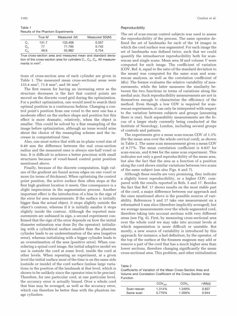
tions of cross-section area of each cylinder are given inTable 1. The measured mean cross-sectional areas were133.4 mm2, 71.8 mm2, and 56 mm2.

The first reason for having an increasing error as thestructure decreases is the fact that control points aremoved on the discrete voxel grid during the optimization.For a perfect optimization, one would need to search theiroptimal position in a continuous fashion. Changing a con-trol point’s position from one voxel to the next one has amoderate effect on the surface shape and position but thiseffect is more dramatic, relatively, when the object issmaller. This could be solved by a fine resampling of theimage before optimization, although an issue would ariseabout the choice of the resampling scheme and the in-crease in computational time.

Also, one must notice that with an in-plane voxel size of0.49 mm the difference between the real cross-sectionradius and the measured ones is always one-half voxel orless. It is difficult to achieve a better precision with smallstructures because of voxel-based control point positionmentioned above.

Finally, because of the discrete computation, high val-ues of the gradient are found across edges on one voxel ormore (in terms of thickness). When optimizing the controlpoint position, the active surface then often stops at thefirst high gradient location it meets. One consequence is aslight imprecision in the segmentation process. Anotherimportant effect is the introduction of a bias in the sign ofthe error for area measurements. If the surface is initiallybigger than the actual object, it stops slightly outside theobject’s contour, whereas if it is initially smaller it stopsslightly inside the contour. Although the reported mea-surements are unbiased in sign, a second experiment con-firmed that the sign of the error depends on how the initialdiameter estimation was done (by the operator): initializ-ing with a cylindrical surface smaller than the phantomcylinder leads to an underestimation of the area (negativeerror), whereas initializing with a bigger cylinder leads toan overestimation of the area (positive error). When con-sidering a spinal cord image, the initial adaptive model weuse is outside the cord at some level, inside the cord atother levels. When repeating an experiment, at a givenlevel the initial surface most of the time is on the same side(outside or inside) of the cord surface (unless large varia-tions in the position of the landmark at that level, which isshown to be unlikely since the operator tries to be precise).Therefore, for one particular cord, at one particular level,the accuracy error is actually biased. Over a whole cordthat bias may be averaged, as well as the accuracy error,which can therefore be better than with the phantom im-age cylinders.

Reproducibility

The set of scan-rescan control subjects was used to assessthe reproducibility of the process. The same operator de-fined the set of landmarks for each of the 18 images inwhich the cord surface was segmented. For each image theset of landmarks was defined twice, such that we couldquantify the intraobserver reproducibility both for scan-rescan and single scans. Mean area M and volume V werecomputed for each image. The coefficient of variation(COV, Ref. 6, equal to the ratio of the standard deviation tothe mean) was computed for the same scan and scan-rescan analyses, as well as the correlation coefficient ofM(s). The former evaluates the relative variability of mea-surements, while the latter measures the similarity be-tween the two functions in terms of variations along themedial axis. Such reproducibility measurements are not inthemselves enough to characterize the efficiency of themethod. Even though a low COV is required for scan-rescan experiments, it can only be interpreted with respectto the variation between subjects and groups (assumingthere is one). Such separability measurements are the fo-cus of a larger study currently being conducted at theInstitute of Neurology, London, including several groupsof controls and patients.

The experiments give a mean scan-rescan COV of 1.3%(for the mean area over the whole cervical cord), as shownin Table 2. The same scan measurement gives a mean COVof 0.77%. The mean correlation coefficient is 0.837 forscan-rescan, and 0.944 for the same scan experiment. Thisindicates not only a good reproducibility of the mean area,but also the fact that the area as a function of a positionalong the cord shows similar variations between two scansof the same subject (see also Figs. 6 and 7).

Although these results are very promising, they indicatea slightly lower reproducibility, or a higher COV, com-pared with the results reported in Refs. 5 and 17. Besidesthe fact that Ref. 17 shows results on the most stable partof the cord, a major difference between our approach andthe ones mentioned above is the possible sources of vari-ability. References 5 and 17 take one measurement on areformatted 5 mm slice (therefore implicitly averaged), butwe average measurements over the whole segmented cord,therefore taking into account sections with very differentareas (see Fig. 6). First, by measuring cross-sectional areaover the whole cord we may take into account levels atwhich segmentation is more difficult or unstable. Butmostly, a new source of variability is introduced by thisapproach: for instance, a bad definition, by the operator, ofthe top of the surface at the foramen magnum may add orremove a part of the cord that has a much higher area thanlower sections, therefore changing significantly the meancross-sectional area. This problem, and other initialization

Table 2Coefficients of Variation of the Mean Cross-Section Area andVolume and Correlation Coefficient of the Cross-Section AreaFunction

COV�M COVV r (M(s))

Scan-rescan 1.314% 1.349% 0.837Same scan 0.770% 1.359% 0.944

Table 1Results of the Phantom Experiments

True M Measured �M Measured SD(M)

C1 131.7 133.406 0.557C2 77 71.795 0.742C3 49.6 55.982 0.754

True cross-section area and measured mean and standard devia-tion of the cross-section area for cylinders C1, C2, C3. All measure-ments in mm2.

1182 Coulon et al.

issues, will be solved by providing better graphical toolswith the software used to define the top and bottom land-marks with respect to other anatomical structures. Never-theless, reproducibility results are comparable to previousmethods and we argue that when examining the entirecord length it is important to also consider the coefficientof correlation.

Table 2 also shows the COV for the volume measure-ments V. One can see that the scan-rescan COV is similar(1.35%) to the one obtained for the mean cross-sectionarea. Nevertheless, the same scan COV is also in the rangeof 1.35% (when one would expect it to be much better),which highlights the fact that volume variation is espe-cially sensitive to the choice of the top and bottom limitsof the cord. This delimitation is, unfortunately, not veryreproducible, especially at the foramen magnum. It re-mains to be seen whether the loss of volume caused by thepresence of atrophy would be significant enough to over-come this variability.

One additional source of intrasubject variability is aslight instability in the segmentation process. The strongdependency on initialization might be an explanation,since this initialization is operator-dependent (with thechoice of the landmarks) and since it does not perform

well for unusual cord shapes. This may be a problem whenthe cord is irregularly deformed by external compression.The problem also comes from the nature of the parameter-ized function. Using spline functions, we have to considera trade-off between quality of the segmentation and com-putational cost, and that trade-off appears in the choice ofthe number of control points (in our case, more than 300).It is worth considering implicit nonparameterized activesurfaces (see, e.g., Ref. 4) and this is the subject of furtherdevelopments of the method. On the other hand, compu-tational cost and difficulties of control during optimizationhave to be balanced with the access to a completely pa-rameterized form that gives access to any differential char-acteristics such as curvatures. As an example, the sameCOV and correlation coefficient statistics were collectedfor the cross-sectional maximum curvature function C(s).Table 3 shows that, in terms of mean reproducibility, theresults are slightly better than the area measurements. Thescan-rescan experiment shows a COV equal to 1.374, sim-ilar to the 1.314 of the cross-section area, and the samescan experiment lead to a COV of 0.540, better than the0.770 found with the area measurements. The correlationcoefficients are worse than with the area measurements(0.727 and 0.800), which can be explained by the fact that

FIG. 6. Plot of the cross-section area as a function of the distancealong the medial axis for two images of the same subject (scan-rescan).

FIG. 7. Plot of the cross-sectional maximum curvature as a functionof the distance along the medial axis for two images of the samesubject (scan-rescan).

Quantification of Spinal Cord Atrophy 1183

C(s) is less smooth than M(s); it shows more variationsalong the axis and therefore is more likely to show a lowcorrelation in the presence of variability between scans.

Potential Application to Other Structures

A promising extension is the application of the samemethod to other structures such as the optic nerve, forquantification of nerve atrophy in cases of optic neuritis(9). Optic nerve MR imaging is difficult due to the size andtortuosity of the nerve, the movements of the eye, and thepresence of high signal from orbital fat and CSF around thenerve. No automatic method is currently available for seg-menting and measuring that structure and we hope tosolve this with further application of our method. A sim-ilar approach may also be useful to study other large pe-ripheral nerves.

CONCLUSION

We have presented a method for segmenting and visualiz-ing the cervical cord. This method gives access to mea-surements of the cross-section area anywhere along itsaxis, whatever the orientation of this axis. The parameter-ized description of the cord surface gives access to differ-ential measurements such as curvature, opening the doorto new types of measurements. Surface rendering andmapping of the measurements on the surface (Fig. 5) canalso be used for visual inspection of the cord. We proposea precise definition of the true orthogonal cross-section ofthe cord, a concept that has not been defined by previousmethods, and which is necessary for providing measure-ments anywhere along the cord (as opposed to semi-localmeasurements averaged over several millimeters along thecord).

A general approach to atrophy detection has been pro-posed and improvements probably mostly reside in in-creasing the quality of segmentation. This will be achievedby investigating other types of active surfaces that canhandle variability of shapes and approximate initializationin a better way, such as implicit surfaces. Geodesic activesurfaces (4), in particular, should handle these featuresand the resulting implicit surface could be parameterizeda posteriori.

Accuracy and reproducibility of the method have beenevaluated and show the method to be viable. In particular,results fully justify the use of our method considering itsadvantages: ease of use, access to the whole cord, no needfor reformatting the data to a particular orientation, andthe possibility of providing other information, such ascurvature. Future studies will investigate the robustness ofthe method in detecting atrophy in a pathological cohort.Preliminary experience in MS suggests that it does (10).

ACKNOWLEDGMENTS

The authors thank Dr. N. Lossef, who acquired the imagesused for the validation of our method. The NMR ResearchUnit is funded by the Multiple Sclerosis Society of GreatBritain and Northern Ireland.

APPENDIX

Definition of the B-Spline Surface

Let v(r,s) � (x(r,s), y(r,s), z(r,s)) be the surface parameter-ization, with s�[0;1] a “longitudinal” parameter, and r�[0;1] an “axial” parameter with v(0,s) � v(1,s) (see, for in-stance, Fig. 2). A cubic B-spline surface patch is defined asfollows. Let P0, P1, …, P15, be a 4 � 4 mesh of controlpoint, with Pi � (Pix, Piy, Piz), and build the control pointmatrix

Gx � �P0x P1x P2x P3x

P4x P5x P6x P7x

P8x P9x P10x P11x

P12x P13x P14x P15x

� , [13]

as well as Gy and Gz defined in the same way. The B-splinebasis matrix MBS, that blends the control points, is definedas follows

MBS � ��

16

12

�12

16

12

�112

0

�12

012

0

16

23

16

0� . [14]

With the two row vectors R � (r3 r2 r 1) and S � (s3 s2 s 1),we can now define the parameterization

x�r, s� � R.M.Gx.MT.ST,

y�r, s� � R.M.Gy.MT.ST, [15]

z�r, s� � R.M.Gz.MT.ST.

Cubic B-spline patches can be put together to form a con-tinuous C2 surface, with the condition that neighboringpatches share 12 control points. Using a cylindrical meshof control points (Fig. 1a), we can define a cylindrical C2

surface made of contiguous B-spline patches (Fig. 1b,c).Every control point in the mesh (except at the top andbottom of the mesh) contributes to the definition of16 different B-spline patches.

REFERENCES

1. Amini A, Curwen RW, Gore JC. Snakes and splines for tracking non-rigid heart motion. Number 1065 in Lecture Notes in ComputerSciences; Berlin: Springer-Verlag; 1996. p 251–261.

2. Amini A, Duncan J. Bending and stretching models for LV wall motionanalysis from curves and surfaces. Image Vis Comput 1992;10:418–430.

Table 3Coefficients of Variation of the Mean Cross-Sectional MaximumCurvature and Correlation Coefficient of the Cross-SectionalMaximum Curvature Function

COV�V R (C(s))

Scan-rescan 1.374% 0.727Same scan 0.540% 0.800

1184 Coulon et al.

3. Do Carmo MP. Differential geometry of curves and surfaces. New York:Prentice Hall; 1976.

4. Caselles V, Kimmel R, Sapiro G. Geodesic active contours. Int J ComputVis 1997;22:61–79.

5. Filippi M, Campi A, Colombo B, Pereira C, Martinelli V, Baratti C, ComiG. A spinal cord MRI study of benign and secondary progressive mul-tiple sclerosis. J Neurol 1996;243:502–505.

6. Goodkin DE, Ross JS, Medendorp SV, Konesci JJ, Rudick RA. Magneticresonance imaging lesion enlargement in multiple sclerosis. Disease-related activity, chance occurrence, or measurement artifact? ArchNeurol 1999;49:261–263.

7. Grossman RI, Barkhof F, Filippi M. Assessment of spinal cord damagein MS using MRI. J Neurol Sci 2000;172:S36–S39.

8. Hackbusch W. Multi-grid methods and applications. Number 4 inSpringer series in computational mathematics; Berlin: Springer-Verlag;1985.

9. Hickman SJ, Brex PA, Brierley CMH, Silver NC, Barker GJ, Scolding NJ,Compston DAS, Moseley IF, Plant GT, Miller DH. Detection of opticnerve atrophy following a single episode of unilateral optic neuritis byMRI using a fat-saturated short-echo fast FLAIR sequence. Neuroradi-ology 2001;43:123–128.

10. Hickman SJ, Coulon O, Parker GJM, Barker GJ, Stevenson VL, ChardDT, Arridge SR, Thompson AJ, Miller DH. Cervical spinal cord volumeestimation using an active surface method: a magnetic resonance im-aging study in multiple sclerosis. In: ECTRIMS’01 European Comitteefor Treatment and Research in Multiple Sclerosis (Abstract), 2001.

11. Hickman SJ, Miller DH. Imaging of the spine in multiple sclerosis.Neuroimag Clin N Am 2000;10:689–704.

12. Kass M, Witkin A, Terzopoulos D. Snakes: active contour models. IntJ Comput Vis 1987;1:321–331.

13. Kidd D, Thorpe JW, Thompson AJ, Kendall BE, Moseley IF, MacManusDG, McDonald WI, Miller DH. Spinal cord MRI using multi-array coilsand fast-spin echo. II. Finding in multiple sclerosis. Neurology 1993;43:2632–2637.

14. Klein AK, Lee F, Amini A. Quantitative coronary angiography withdeformable spline models. IEEE Trans Med Imag 1997;16:468–482.

15. Liao CW, Medioni G. Representation of range data with B-spline sur-face patches. In: 11th Int Conf on Pattern Recognition, Volume III,conference C: Image, Speech, and Signal Analysis; 1992. p 745–748.

16. Lossef NA, Miller DH. Measures of brain and spinal cord atrophy inmultiple sclerosis. J Neurol Neurosurg Psychiatry 1998;64:S102–S105.

17. Lossef NA, Webb SL, O’Riordan JI, Page R, Wang L, Barker GJ, Tofts PS,McDonald WI, Miller DH, Thompson AJ. Spinal cord atrophy anddisability in multiple sclerosis. A new reproducible and sensitive MRImethod with potential to monitor disease progression. Brain 1996;119:701–708.

18. McInerney T, Terzopoulos D. Deformable models in medical imageanalysis: a survey. Med Image Anal 1996;1:91–108.

19. Morse BS. Computation of object cores from grey-level images. Ph.D.thesis, University of North Carolina at Chapel Hill, 1994.

20. Schnabel J, Arridge SR. Active shape focusing. Image Vis Comput1999;17:419–428.

21. Williams DJ, Shah M. A fast algorithm for active contours and curva-ture estimation. Comput Vis Graph Image Proc: Image Understand1992;55:14–26.

Quantification of Spinal Cord Atrophy 1185