Journal of Computational and Applied Mathematics 221 (2008) 367–375www.elsevier.com/locate/cam

On the construction of local quadratic spline quasi-interpolants onbounded rectangular domains

C. Dagnino, P. Lamberti∗

Department of Mathematics, University of Torino, via C.Alberto, 10 - 10123 Torino, Italy

Received 19 December 2006; received in revised form 25 May 2007

Abstract

In this paper local bivariate C1 spline quasi-interpolants on a criss-cross triangulation of bounded rectangular domains areconsidered and a computational procedure for their construction is proposed. Numerical and graphical tests are provided.c© 2007 Elsevier B.V. All rights reserved.

MSC: 65D07; 65D15; 41A15

Keywords: Spline approximation; Quasi-interpolation; Criss-cross triangulation; Algorithms

1. Introduction

Let � = [a, b] × [c, d] be a rectangular domain, decomposed into mn subrectangles by the two partitions

Xm = {xi , 0 ≤ i ≤ m}, Yn = {y j , 0 ≤ j ≤ n},

of the segments [a, b] = [x0, xm] and [c, d] = [y0, yn], respectively. The so called criss-cross triangulationTmn of � is defined by drawing the two diagonals in each subrectangle. We define S1

2(Tmn) = {s ∈ C1(�):the restriction of s to each triangle is an element of P2}, where P` is the space of polynomials in two variables of totaldegree less than or equal to `.

Let also {Bi j , (i, j) ∈ Kmn}, with Kmn = {(i, j) : 0 ≤ i ≤ m + 1, 0 ≤ j ≤ n + 1}, be the collection of(m + 2)(n + 2)B-splines [1,4,17], with knots:

x−2 ≤ x−1 ≤ a = x0 < x1 < · · · < xm = b ≤ xm+1 ≤ xm+2,

y−2 ≤ y−1 ≤ c = y0 < y1 < · · · < yn = d ≤ yn+1 ≤ yn+2,(1)

that generate the space S12(Tmn). They can be computed both in piecewise polynomial (pp) form, by using the

conformality condition method [3], and in Bernstein–Bezier (B–B) form [12].

∗ Corresponding author.E-mail addresses: catterina.dagnino@unito.it (C. Dagnino), paola.lamberti@unito.it (P. Lamberti).

0377-0427/$ - see front matter c© 2007 Elsevier B.V. All rights reserved.doi:10.1016/j.cam.2007.10.025

368 C. Dagnino, P. Lamberti / Journal of Computational and Applied Mathematics 221 (2008) 367–375

Fig. 1. Some supports of B-splines with (a) simple knots and (b) multiple knots on ∂�.

Since dim S12(Tmn) = (m + 2)(n + 2) − 1 and there is only one linear dependency among the Bi j ’s, then a basis

for S12(Tmn) is obtained by deleting any one of them [3].

If in (1) we assume

x−2 < x−1 < a, b < xm+1 < xm+2,

y−2 < y−1 < c, d < yn+1 < yn+2,(2)

then we obtain the so called “classical” B-splines with octagonal support Σi j , simple knots and C1 smoothnesseverywhere [3]. We remark that some of their supports are not completely included in �, as shown in Fig. 1(a).

If, in (1), we assume

x−2 ≡ x−1 ≡ a, b ≡ xm+1 ≡ xm+2,

y−2 ≡ y−1 ≡ c, d ≡ yn+1 ≡ yn+2,(3)

then we have a new set of B-splines Bi j [13,15] with multiple knots on the boundary ∂� of � and all supports Σi jincluded in � (Fig. 1(b)). We denote it by Bmn . Like the “classical” B-splines, the new ones also satisfy the partitionof unity property.

We can distinguish three kinds of “modified” Bi j ’s belonging to Bmn . There are:(i) a first-boundary-layer of 2m + 2n + 4 B-splines, with triple knots on ∂�, i.e.: Bi0, Bi,n+1, 0 ≤ i ≤

m + 1, B0 j , Bm+1, j , 1 ≤ j ≤ n;(ii) a second-boundary-layer of 2m + 2n − 4 B-splines, with double knots on ∂�, i.e.: Bi1, Bin, 1 ≤ i ≤

m, B1 j , Bmj , 2 ≤ j ≤ n − 1;(iii) (m − 2)(n − 2) inner B-splines, with simple knots, i.e.: Bi j , 2 ≤ i ≤ m − 1, 2 ≤ j ≤ n − 1, coinciding with

the corresponding “classical” ones.The knot multiplicity affects the B-spline smoothness, i.e. Bi j is 2 − r differentiable, if r is the knot multiplicity.

Therefore the first-boundary-layer B-splines have a jump on ∂�, the second-boundary-layer ones are C0 on ∂� andthe inner ones are C1 everywhere. Moreover they can be expressed in terms of “classical” B-splines [8].

We recall [6] that the second-boundary-layer B-splines and the inner ones coincide with the so called“interior”, “side” and “corner” B-splines, spanning the space of C1 quadratic piecewise polynomials with boundaryconditions [2].

Figs. 2–5 show some B-splines with (a) simple knots and (b) multiple knots on ∂�.This paper deals with discrete local quadratic spline quasi-interpolants (q-i’s), defined on a criss-cross triangulation

Tmn of � and generated by the B-splines belonging to Bmn .In Section 2 we introduce the spline q-i’s and we recall some of their properties. In Section 3 we propose a

procedure, developed in Matlab, for their generation and we give numerical and graphical test results.

2. Local quadratic C1 spline quasi-interpolants

We consider linear operators

Q : C(�) → S12(Tmn),

C. Dagnino, P. Lamberti / Journal of Computational and Applied Mathematics 221 (2008) 367–375 369

Fig. 2. (a) The “classical” B-spline B00 on Σ00 ∩ �; (b) the first-boundary-layer B-spline B00 on Σ00 with triple knots on both x and y axis.

Fig. 3. (a) The “classical” B-spline B10 on Σ10 ∩ �; (b) the first-boundary-layer B-spline B10 on Σ10 with triple and double knots on the x andy axis, respectively.

defined by

Q f (x, y) =

∑(i, j)∈Kmn

λi j f Bi j (x, y), (4)

where the knot partitions are given by (1) with the choice (3), Bi j ∈ Bmn, ∀(i, j) ∈ Kmn , as introduced in Section 1,and λi j : C(�) → R is a discrete linear functional of the following form:

λi j f =

p∑µ=1

wµ f (x (i)µ , y( j)

µ ), (5)

involving only a finite fixed number p ≥ 1 of triangular mesh-points (x (i)µ , y( j)

µ ) either in the support Σi j or close to itand of real non-zero weights wµ. Moreover the λi j ’s are assumed to be such that Q f = f for all f ∈ P`, 0 < ` ≤ 2.

Therefore such an operator Q is a quasi-interpolant [4] and it defines a local approximation scheme, because thevalue of Q f (x, y) depends only on the values of f in a neighborhood of (x, y). Indeed if we assume (t, t) ∈ � and if

370 C. Dagnino, P. Lamberti / Journal of Computational and Applied Mathematics 221 (2008) 367–375

Fig. 4. (a) The “classical” B-spline B11 on Σ11 ∩ �; (b) the second-boundary-layer B-spline B11 on Σ11 with double knots on both x and y axis.

Fig. 5. (a) The “classical” B-spline B21 on Σ21 ∩ �; (b) the second-boundary-layer B-spline B21 on Σ21 with double and simple knots on the xand y axis, respectively.

T is the triangular cell of Tmn containing (t, t), since just seven B-splines Bi j are non-zero on T , then it results that

Q f (t, t) =

∑i, j /

T ∩ Σi j 6=∅

λi j f Bi j (t, t). (6)

Now we consider some interesting spline q-i’s of the kind of (4), given in [8,13,15]. In order to introduce them, weneed the following notation.

For 0 ≤ i ≤ m + 1 and 0 ≤ j ≤ n + 1 we set hi = xi − xi−1, k j = y j − y j−1,

ai = −σ 2

i σ ′

i+1

σi + σ ′

i+1, ci = −

σi (σ′

i+1)2

σi + σ ′

i+1, a j = −

τ 2j τ

′

j+1

τ j + τ ′

j+1, c j = −

τ j (τ′

j+1)2

τ j + τ ′

j+1,

bi j = 1 − (ai + ci + a j + c j ),

C. Dagnino, P. Lamberti / Journal of Computational and Applied Mathematics 221 (2008) 367–375 371

Fig. 6. Function evaluation points involved by: (a) the functionals (i) and (ii); (b) the functionals (iii). The symbol ◦ denotes a multiple knot.

with a0 = c0 = am+1 = cm+1 = a0 = c0 = an+1 = cn+1 = 0, b00 = b0,n+1 = bm+1,0 = bm+1,n+1 = 1 and

σi =hi

hi−1 + hi, σ ′

i = 1 − σi , τ j =k j

k j−1 + k j, τ ′

j = 1 − τ j .

For any f ∈ C(�), the following choices of functionals of the kind of (5):

(a) λi j f = f (Mi j ),

(b) λi j f = bi j f (Mi j ) + ai f (Mi−1, j ) + ci f (Mi+1, j ) + a j f (Mi, j−1) + c j f (Mi, j+1),

(c) λi j f = 2 f (Mi j ) −14

0∑h=−1

0∑k=−1

f (Ai+h, j+k),

(7)

where Mi, j = (si , t j ), with si =12 (xi−1 + xi ), t j =

12 (y j−1 + y j ), and Ars = (xr , ys), − 1 ≤ r ≤ m + 1, − 1 ≤

s ≤ n + 1 (Fig. 6), allow us to define the corresponding spline q-i’s (4), that we denote by S1, S2 and W2, respectively.The number of data sites is equal to NS(m, n) = (m +2)(n +2) for S1, S2 and to NW (m, n) = 2mn +3m +3n +1

for W2.We recall [8,13,15] that the infinite norms of the operators S1, S2 and W2 are uniformly bounded. Moreover S1

reproduces bilinear polynomials, while S2 and W2 are exact for P2 in �. Therefore Q can approximate real functionsand their partial derivatives of first and second order up to a near optimal order if Q = S1 and to an optimal order ifQ = S2 and W2. For such splines, convergence properties and error upper bounds in terms of the smoothness of fand of the characteristics of the triangulation have also been derived [8].

Moreover quasi-interpolants (4), defined by means of “modified” B-splines, interpolate the function f at the fourvertices of the domain � and they need function evaluation points all contained both inside the domain � and on ∂�.Finally it has been shown [6] that they can be directly used to provide splines with boundary conditions.

We recall that similar operators, based on “classical” B-splines [3], have been defined and studied in theliterature [4,5,17]. However they haven’t the performances of the ones above; for instance they need functionevaluation points also outside � and they cannot be directly used for boundary condition splines.

3. A computational procedure and numerical results

In this section we present a general procedure for constructing a local discrete spline q-i of the kind of (4), wherethe “modified” B-splines Bi j are computed by means of their B-nets.

The code [7], developed in the convenient interactive environment that MATLAB provides, is modularized in afashion similar to that of the structure of the Spline Toolbox function M-files [16] and it is available. All computationshave been carried out on a personal computer, with a 16-digit arithmetic.

Our main user-callable function M-files are the following:– bijdec. Given in input the knots, defined by (1) with the choice (3), a point (u, v) in � and two integers i and j ,

the procedure returns the value of Bi j (u, v), computed by means of its B-net [14] and the de Casteljau algorithm [9].– qinterp. Given in input the knots, defined by (1) with the choice (3), the matrix {λi j f } defined by (5) and an

arbitrary grid u × v of evaluation points in �, the procedure returns the values of the bivariate spline Q f at u × v,according to (6). It calls bijdec.

372 C. Dagnino, P. Lamberti / Journal of Computational and Applied Mathematics 221 (2008) 367–375

Other minor M-files are utilities that perform the visualization of Q f , {Bi j } (Figs. 2–5(b)) and the constructionand the visualization of the supports {Σi j } (Fig. 1(b)).

We remark that the construction of first-boundary-layer and second-boundary-layer of B-splines doesn’t involvespecial numerical difficulties. Indeed their B-nets are computed using those of the corresponding “classical” B-splines [14], putting to zero the length of the support intervals that are “degenerate” because of multiple knots.

We tested our procedure for the discrete spline q-i’s S1, S2 and W2, defined by the functionals (7). In order todo this, two function M-files ls2 and lw2 are proposed. Given as input the knot partitions, defined by (1) with thechoice (3), and the matrix { f (Mi j )} (the matrices { f (Mi j )} and { f (Ars)}), ls2 (lw2) returns the matrix {λi j f } of thefunctionals (7) for S2 (W2). We remark that, for S1, the matrix {λi j f } coincides with the matrix { f (Mi j )}. Matrices{λi j f }, corresponding to other choices of functionals of the kind of (5), can be provided by the user.

We used several test functions, usually considered in approximation algorithms ([11] et al.). Here, we proposesome results obtained for the following ones:

– f1(x, y) = (r − 0.6)4+ where r =

√x2 + y2;

– f2(x, y) =19

√64 − 81((x −

12 )2 + (y −

12 )2) −

12 ;

– f3(x, y) = e−(5−10x)2

2 + 0.75e−(5−10y)2

2 + 0.75e−(5−10x)2

2 e−(5−10y)2

2 ;

– f4(x, y) =

{|x |y if xy > 00 elsewhere.

All functions are approximated on the unit square, except the last one, studied in [−1, 1]× [−1, 1]. We remark thatfor such functions the maximum norms are 0.439, 0.389, 2.500, 1, respectively. The function f2 is a well-knownFranke’s test function. Some test functions are smooth; some others, e.g. f3, have multiple features and abrupttransitions, so they are quite challenging. For this reason we considered several choices of domain partitions bymaking many subdivisions in the vicinity of a function high variation or irregularity. In order to do this, for the hereproposed functions, we use one of the following three types of domain partitions:

P(k)m,n = Xm × Yn = {(xi , y j )}

= {((b − a)ξ(k)i + a, (d − c)η(k)

j + c)}, k = 1, 2, 3, (8)

with

(1) ξ(1)i =

15 sin m−i

m π +im , η

(1)j =

15 sin n− j

n π +jn , i = 0, . . . , m, j = 0, . . . , n;

(2) ξ(2)i =

12 (cos m−i

m π + 1), η(2)j =

12 (cos n− j

n π + 1), i = 0, . . . , m, j = 0, . . . , n;

(3) ξ(3)i =

12 cos m/2−i

m π , η(3)j =

12 cos n/2− j

n π , i = 0, . . . , m/2, j = 0, . . . , n/2 and

ξ(3)i = 1 − ξ

(3)m−i , η

(3)j = 1 − η

(3)n− j , i = m/2 + 1, . . . , m, j = n/2 + 1, . . . , n (m, n even).

Operators based on “modified” B-splines have been compared with similar ones, based on “classical” B-splines,from a graphical and numerical point of view. The graphical rendering is the same in both cases.

In Figs. 7–10 the graphs of spline q-i’s, based on “modified” B-splines and approximating the above test functions,are displayed with the corresponding points of the selected type of domain partition, where for the sake of clarity onlythe triangular mesh-points appear.

Regarding the numerical aspects, the maximum absolute errors, computed using a 55 × 55 uniform rectangulargrid of evaluation points in the domain �, are reported in Tables 1–4 for increasing values of m and n. The measureof the error is given by E Q = ‖ f − Q f ‖∞ with Q ≡ S1, S2, W2, S(c)

1 , W (c)2 where (c) denotes spline q-i’s based

on “classical” B-splines [17]. Moreover, on one hand a comparison is carried out on the same spline space S12(Tmn);

on the other hand, since NS(m, n) < NW (m, n) and in particular NS(m, n) = O(mn), while NW (m, n) = O(2mn),we also compare the two operators S2 and W2, by using about the same number of function evaluations. In order to

do this, since NS(m, n) ≈ NW

(⌈m√

2

⌉,⌈

n√

2

⌉), we assume S2 defined on Tmn and W2 defined on T⌈

m√

2

⌉,⌈

n√

2

⌉.

C. Dagnino, P. Lamberti / Journal of Computational and Applied Mathematics 221 (2008) 367–375 373

Fig. 7. (a) S1 f1 and (b) P(1)8,8 .

Fig. 8. (a) S2 f2 and (b) P(2)8,8 .

Table 1Maximum absolute errors for f1

m = n E S(c)1 E S1 E S2 EW2, EW (c)

2 EW2 with T⌈m√

2

⌉,⌈

n√2

⌉4 1.87(−2) 1.75(−2) 2.97(−3) 2.26(−3) 6.82(−3)

8 4.81(−3) 4.66(−3) 2.92(−4) 2.66(−4) 7.64(−4)

16 1.20(−3) 1.19(−3) 2.54(−5) 2.14(−5) 6.46(−5)

32 3.00(−4) 2.97(−4) 2.22(−6) 2.32(−6) 6.76(−6)

64 7.51(−5) 7.45(−5) 2.90(−7) 2.99(−7) 7.35(−7)

The analysis of all tests shows that spline q-i’s, based on “modified” B-splines, are comparable with the ones basedon “classical” ones. However the first ones do not need any function evaluation points outside the domain � and they

374 C. Dagnino, P. Lamberti / Journal of Computational and Applied Mathematics 221 (2008) 367–375

Fig. 9. (a) W2 f3 and (b) P(3)16,16.

Table 2Maximum absolute errors for f2

m = n E S1, E S(c)1 E S2 EW2 EW (c)

2

4 3.58(−2) 2.88(−3) 3.39(−3) 3.39(−3)

8 1.03(−2) 3.48(−4) 2.55(−4) 2.55(−4)

16 2.68(−3) 3.41(−5) 2.11(−5) 2.11(−5)

32 6.75(−4) 2.77(−6) 1.92(−6) 1.92(−6)

64 1.69(−4) 2.32(−7) 2.09(−7) 2.13(−7)

Table 3Maximum absolute errors for f3

m = n E S1, E S(c)1 E S2 EW2 EW (c)

2 EW2 with T⌈m√

2

⌉,⌈

n√2

⌉4 7.22(−1) 6.03(−1) 5.3275(−1) 5.3262(−1) –8 1.97(−1) 1.03(−1) 1.12(−1) 1.12(−1) 1.37(−1)

16 5.58(−2) 1.22(−2) 9.72(−3) 9.72(−3) 2.86(−2)

32 1.59(−2) 1.07(−3) 7.55(−4) 7.55(−4) –64 4.00(−3) 1.14(−4) 8.74(−5) 8.74(−5) 2.77(−4)

Table 4Maximum absolute errors for f4

m = n E S(c)1 E S1 E S2 EW2 EW (c)

2 EW2 with T⌈m√

2

⌉,⌈

n√2

⌉4 8.18(−2) 7.32(−2) 5.96(−2) 7.32(−2) 8.18(−2) –8 1.90(−2) 1.90(−2) 1.57(−2) 1.90(−2) 1.90(−2) 3.34(−2)

16 4.80(−3) 4.80(−3) 3.99(−3) 4.80(−3) 4.80(−3) 8.51(−3)

32 1.20(−3) 1.20(−3) 1.00(−3) 1.20(−3) 1.20(−3) –64 3.01(−4) 3.01(−4) 2.50(−4) 3.01(−4) 3.01(−4) 5.82(−4)

interpolate f at the four vertices of �. As we have already underlined, such properties, together with the classicalones of locality and handling easiness, turn out to be very useful in many applications, for instance in approximationwith boundary conditions [6], in numerical integration [10], etc.

C. Dagnino, P. Lamberti / Journal of Computational and Applied Mathematics 221 (2008) 367–375 375

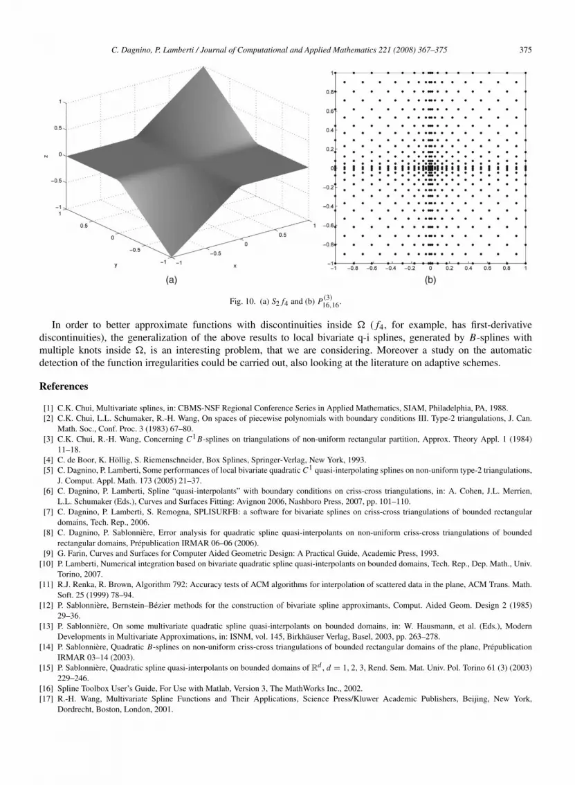
Fig. 10. (a) S2 f4 and (b) P(3)16,16.

In order to better approximate functions with discontinuities inside � ( f4, for example, has first-derivativediscontinuities), the generalization of the above results to local bivariate q-i splines, generated by B-splines withmultiple knots inside �, is an interesting problem, that we are considering. Moreover a study on the automaticdetection of the function irregularities could be carried out, also looking at the literature on adaptive schemes.

References

[1] C.K. Chui, Multivariate splines, in: CBMS-NSF Regional Conference Series in Applied Mathematics, SIAM, Philadelphia, PA, 1988.[2] C.K. Chui, L.L. Schumaker, R.-H. Wang, On spaces of piecewise polynomials with boundary conditions III. Type-2 triangulations, J. Can.

Math. Soc., Conf. Proc. 3 (1983) 67–80.[3] C.K. Chui, R.-H. Wang, Concerning C1 B-splines on triangulations of non-uniform rectangular partition, Approx. Theory Appl. 1 (1984)

11–18.[4] C. de Boor, K. Hollig, S. Riemenschneider, Box Splines, Springer-Verlag, New York, 1993.[5] C. Dagnino, P. Lamberti, Some performances of local bivariate quadratic C1 quasi-interpolating splines on non-uniform type-2 triangulations,

J. Comput. Appl. Math. 173 (2005) 21–37.[6] C. Dagnino, P. Lamberti, Spline “quasi-interpolants” with boundary conditions on criss-cross triangulations, in: A. Cohen, J.L. Merrien,

L.L. Schumaker (Eds.), Curves and Surfaces Fitting: Avignon 2006, Nashboro Press, 2007, pp. 101–110.[7] C. Dagnino, P. Lamberti, S. Remogna, SPLISURFB: a software for bivariate splines on criss-cross triangulations of bounded rectangular

domains, Tech. Rep., 2006.[8] C. Dagnino, P. Sablonniere, Error analysis for quadratic spline quasi-interpolants on non-uniform criss-cross triangulations of bounded

rectangular domains, Prepublication IRMAR 06–06 (2006).[9] G. Farin, Curves and Surfaces for Computer Aided Geometric Design: A Practical Guide, Academic Press, 1993.

[10] P. Lamberti, Numerical integration based on bivariate quadratic spline quasi-interpolants on bounded domains, Tech. Rep., Dep. Math., Univ.Torino, 2007.

[11] R.J. Renka, R. Brown, Algorithm 792: Accuracy tests of ACM algorithms for interpolation of scattered data in the plane, ACM Trans. Math.Soft. 25 (1999) 78–94.

[12] P. Sablonniere, Bernstein–Bezier methods for the construction of bivariate spline approximants, Comput. Aided Geom. Design 2 (1985)29–36.

[13] P. Sablonniere, On some multivariate quadratic spline quasi-interpolants on bounded domains, in: W. Hausmann, et al. (Eds.), ModernDevelopments in Multivariate Approximations, in: ISNM, vol. 145, Birkhauser Verlag, Basel, 2003, pp. 263–278.

[14] P. Sablonniere, Quadratic B-splines on non-uniform criss-cross triangulations of bounded rectangular domains of the plane, PrepublicationIRMAR 03–14 (2003).

[15] P. Sablonniere, Quadratic spline quasi-interpolants on bounded domains of Rd , d = 1, 2, 3, Rend. Sem. Mat. Univ. Pol. Torino 61 (3) (2003)229–246.

[16] Spline Toolbox User’s Guide, For Use with Matlab, Version 3, The MathWorks Inc., 2002.[17] R.-H. Wang, Multivariate Spline Functions and Their Applications, Science Press/Kluwer Academic Publishers, Beijing, New York,

Dordrecht, Boston, London, 2001.