IEEE TRANSACTIONS ON MAGNETICS, VOL. 41, NO. 6, JUNE 2005 2077

Demagnetizing Factors for Rectangular PrismsD.-X. Chen1, E. Pardo2, and A. Sanchez2

ICREA and Grup d’Electromagnetisme, Departament de Física, Universitat Autònoma de Barcelona,08193 Bellaterra, Barcelona, Spain

Grup d’Electromagnetisme, Departament de Física, Universitat Autònoma de Barcelona, 08193 Bellaterra, Barcelona, Spain

For rectangular prisms of dimensions 2 2 2 with constant material susceptibility , we have calculated and tabulated thefluxmetric and magnetometric demagnetizing factors and , defined along the 2 dimension as functions of ( )1 2(=1500) (=1 256) and (=0 109). We introduce an interpolation technique for obtaining with arbitrary values of( )1 2 and .

Index Terms—Demagnetizing correction, fluxmetric demagnetizing factor, magnetometric demagnetizing factor, magnetic measure-ments, rectangular prisms.

I. INTRODUCTION

WHEN a body is placed in a uniform applied field ,it is magnetized not only by but also by the field

produced by the resultant magnetic poles in the body itself. Thefield produced by such poles is usually called the demagnetizingfield . Assuming the material to have a constant suscepti-bility for the sake of simplicity, the magnetic poles can bepresent only on the body surface and they appear only whenthere are some surfaces not parallel to the applied field. Since

and so the magnetization are generally nonuniform anddepend on both and body shape, the demagnetizing effectsmay bring about great complexities in the magnetic measure-ments of materials [1]–[3].

In order to avoid such effects, toroidal samples are recom-mended in magnetic measurements of soft and semi-soft mag-netic materials. In this case, the sample is magnetized by a cur-rent- carrying coil uniformly wound on to it, so that the entiresample surface is parallel to the circular applied field and thedemagnetizing field is absent at a sacrifice of the uniformity ofthe circular applied field, which is inversely proportional to thedistance to the axis of cylindrical symmetry of the sample. Themaximum circular field that can be applied is on the order of10 kA/m, which is limited by the allowed maximum tempera-ture rise. For semi-soft magnetic materials, one can use a per-meameter to measure a single tape, whose both ends are welltouched to a yoke made of soft-magnetic lamination, forminga closed magnetic circuit. When a uniformly wound current-carrying solenoid surrounds the tape, the demagnetizing fieldsproduced by the poles appearing in both end regions will bepartially cancelled by the fields produced by the poles inducedin the yoke with signs opposite to those in the tape ends. Themaximum field in such single tape measurements can be severaltimes greater than that in ring sample measurements. For hardmagnetic materials requiring a maximum field of the order ofMA/m, the recommended sample shapes are cylinders or rect-angular prisms and the magnetizer is usually an electromagnet.In this case, the fields produced by the induced poles in soft-magnetic pole pieces of the magnet will also reduce the demag-netizing field in the sample [1], [2].

Digital Object Identifier 10.1109/TMAG.2005.847634

In contrast to the above examples where demagnetizing fieldsare reduced or eliminated, there has been another way to dealwith the demagnetizing problem in magnetic measurements,which is to calculate demagnetizing factors for certain sampleshapes. In this case, the sample made of material with a con-stant susceptibility and having a certain symmetric shape isplaced in a uniform , and if the average magnetizationin the sample is parallel to along the symmetry axis and sois the average demagnetizing field , then the average de-magnetizing factor is defined as . If thebody shape is ellipsoidal, and are uniform, so thatis reduced to a simple demagnetizing factor , which is a func-tion of the aspect ratios of the sample but independent of andwas analytically calculated a long time ago [4]. For any othershapes, one has to define how the average is made and willdepend not only on aspect ratios but also on . Correspondingto magnetometric and fluxmetric measurements, the average isconventionally made over the entire body volume and over themidplane, and the ’s are referred to as the magnetometricand fluxmetric demagnetizing factors, and , respectively[3]. If values are available, may be calculated from thedirectly measured external susceptibility of the sample, de-fined by . In fact, in the research and develop-ment of magnetic materials, wires, cylinders, and rectangulartapes and blocks are often the most convenient sample shapes,and they may be easily magnetized by a current-carrying sole-noid, so that the calculation of demagnetizing factors is neces-sary in practice.

The numerical calculations of for different sampleshapes with different aspect ratios and have formed a centuryold topic [3]. However, a practically complete set of resultswas obtained just a decade ago for one shape, cylinder, thanksto the developments of computer technology [3]. For anotherimportant geometry, rectangular prism, there have long beenanalytical results of for the general three-dimensionalcase for and analytical transverse for infinitelylong bars for [5]–[8]. For these latter bars, transverse

as functions of and the transverse aspect ratio havebeen calculated recently [9], [10]. Since a complete functionalthree-dimensional calculation is too complicated, we have cal-culated the axial of square bars as functions of the aspectratio and to compare with the existing results of cylinders,

0018-9464/$20.00 © 2005 IEEE

2078 IEEE TRANSACTIONS ON MAGNETICS, VOL. 41, NO. 6, JUNE 2005

and of rectangular prisms as functions of aspect ratios forthe case of for applications in superconductors [11],[12]. In the present paper, we will give of rectangularprisms as functions of aspect ratios and , relevant to themeasurements of various magnetic materials. Different fromthe results given in [3], [10]–[12], where only tables of discretedata points are present and functional curves are plotted di-rectly from the data in the tables, we will introduce an accurateinterpolation technique in detail, so that the resultant areactually presented as continuous functions of aspect ratios and

in a wide range. This will provide readers who need to makedemagnetizing corrections for their sample having any valuesof aspect ratios and with relevant correct . Moreover,we will introduce an iteration technique in detail, so that thefinal and of the sample can be obtained from thedirectly measured and aspect ratios.

Although the method and formulas for the present calcula-tions have already been given in [11] and [12], we will make anecessary description on them in Section II, commenting on thereasons for the steps and conditions we have used in this work.Although these reasons are stated in a logical way, they were notrealized a priori but concluded from the success and failure ofour long-term intensive work. Thus, we expect that such a de-scription can be practically useful to those who are dealing withdemagnetizing problems. The results of will be presentedas tables and figures in Section III. Section IV will be devoted tothe discussion and application of the results and our conclusionswill be stated in Section V. In the Appendix, we summarize thequantities appearing in the paper for facilitating the readers.

II. CALCULATION

A. Magnetostatic Problem of Rectangular Prism

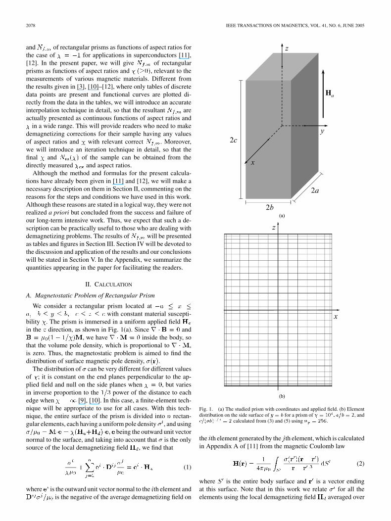
We consider a rectangular prism located atwith constant material suscepti-

bility . The prism is immersed in a uniform applied fieldin the direction, as shown in Fig. 1(a). Since and

, we have inside the body, sothat the volume pole density, which is proportional to ,is zero. Thus, the magnetostatic problem is aimed to find thedistribution of surface magnetic pole density, .

The distribution of can be very different for different valuesof ; it is constant on the end planes perpendicular to the ap-plied field and null on the side planes when , but variesin inverse proportion to the power of the distance to eachedge when [9], [10]. In this case, a finite-element tech-nique will be appropriate to use for all cases. With this tech-nique, the entire surface of the prism is divided into rectan-gular elements, each having a uniform pole density , and using

being the outward unit vectornormal to the surface, and taking into account that is the onlysource of the local demagnetizing field , we find that

(1)

where is the outward unit vector normal to the th element andis the negative of the average demagnetizing field on

Fig. 1. (a) The studied prism with coordinates and applied field. (b) Elementdistribution on the side surface of y = b for a prism of � = 10 ; a=b = 2, andc=(ab) = 2 calculated from (3) and (5) using n = 256.

the th element generated by the th element, which is calculatedin Appendix A of [11] from the magnetic Coulomb law

(2)

where is the entire body surface and is a vector endingat this surface. Note that in this work we relate for all theelements using the local demagnetizing field averaged over

CHEN et al.: DEMAGNETIZING FACTORS FOR RECTANGULAR PRISMS 2079

the surface of each element, rather than using at the center ofeach element as done in [3] and [10]. This modification allowsus to improve appreciably the accuracy of calculated forprisms to a level higher than that for cylinders calculated in [3].Otherwise, the pole distribution of a prism (having 12 edges) ismuch more difficult to be calculated accurately than that of acylinder (having only two edges) [7], [13].

The set of linear equations (1) should include as many un-known variables as the number of elements covering the en-tire surface. However, as done in [10], the number of unknownvariables can be reduced by considering the symmetry. To doso, we take for the elements within the regionas unknown variables and we include the contributions toof the eight different elements at symmetric positions with thesame magnitude of surface pole density in the matrix . Theresultant set of linear equations is solved using the LU decom-position routine [14].

B. Surface Element Division

The division of the surface into elements is done as follows.The elements are taken to be rectangular shaped. Their size inthe direction depends only on the coordinate of the po-sition of the element center depends only on , anddepends only on . In this way, the surface division into ele-ments can be done as the composition of three independent lineelement divisions. We take the same nonlinear line division inthe direction as done in [10] for the direction parallel to theapplied field. Consistently, the line divisions in the and di-rections are done as in [10] for the direction perpendicular to thefield. A more detailed description is made as follows.

As derived in [9], when tends to infinity aspower over the distance to the edge. Since at high aremost difficult to be calculated accurately, the surface elementdistribution should be made based on this law. Improving thecalculation for cylinders, where a basically uniform pole in-tensity for is made in the elements near the edges, aroughly uniform pole-density increment for is imple-mented near the edges for the present calculation. As in [10],we use artificial distributions

(3)

(4)

(5)

to calculate the element divisions along the , and direc-tions, respectively. In order to overcome the difficulty arisingfrom the actually infinite at the edges, we extend the , and

for small lengths , and , so that the , andcalculated from (3)–(5) are large finite numbers. Thus, the

division units become, and . The proper values of

, and are chosen for different values of

and aspect ratios in such a way that the minimum error in thecalculated is obtained.

The numbers of divisions in the three directions, ,and (with a layer riding on the midplane with

, which is essential for reducing the error of the final results,especially for ), are taken by fixing the number of elementsintegrally belonging to the region,

, selecting(this is tested to be a proper choice independent of the valueof ), and assuming . The elements centeredat have , so that on these elements are notunknown variables. We also consider a restriction for

. This restriction ensures sufficiently fine divisionswhen is very large so that a minimum error in the final

is reached.An exemplified element division on a side surface for a prism

of , and is shown in Fig. 1(b).In order to have a sufficient resolution near the edges,

is used with and . In the actualcalculation, is set as large as 4800.

C. Calculation of

The fluxmetric and magnetometric demagnetizing factors,and , are defined by [3]

(6)

where the subscripts “mid” and “vol” stand for the average overthe midplane and over the entire volume, respectively. Whenthe prism material has a constant as in the present case, thedemagnetizing factors can be calculated from eitheror using [10]

(7)

(8)

Using the calculated surface pole density, can beeasily calculated by the surface integration of , using

inside the body and on the surface [3], [10].may be calculated from the sum of the prism-mid-

plane (at ) and prism-volume averaged fields generated byall rectangular elements as

(9)

(10)

where and are the prism-midplane average andprism-volume average of the component of the magnetic fieldper unit generated by the th element at ,whose analytical expressions may be obtained from the for-mulas derived in Appendixes A and B of [11]. The use of ana-lytical formulas for avoids doing numerical midplaneand volume integrations, as done in [3], [10], so it avoids pos-sible extra numerical error for calculations and savesaround 50% of the total computer time.

2080 IEEE TRANSACTIONS ON MAGNETICS, VOL. 41, NO. 6, JUNE 2005

D. Correction of

The demagnetizing factors can be calculated from ei-ther or using (7) and (8), respectively. If

is calculated in both ways, we can obtain a corrected. The correction formula is

(11)

where is the value of calculated using andis obtained by means of .

Using the finite-element method, there is always a discretiza-tion error in the calculated pole density distribution, especiallywhen is large so that shows a sharp divergence near theedges. When calculating of cylinders [3], we found thatthe calculated were very sensitive to the element divi-sion and that and calculated from the same distri-bution could be orders of magnitude different from each othereven if quite a large element number was used. This became avital problem that seriously limited the accuracy of the resultsof . After carefully investigating (7) and (8), we found thata small error in and could result in a greaterror in and . Then, reasonably assuming the rela-tive errors in the calculated and owing tothe discretization in the pole distribution to be the same

(12)

where quantities with a superscript denote their ideal correctvalues whereas those without a superscript denote their calcu-lated values with some error, a correction formula (11) was de-rived from (7) and (8). Compared with the directly calculated

and , the error of the corrected was at leastone order of magnitude smaller. The validity of such a correc-tion technique has been further justified in [10] and used in [11],[12]. In the present work, all the final data for are actually

.

E. Error Estimation

In a previous work [10], the error in the calculated waschecked by comparing the results with those calculated analyti-cally for several values. However, for the case of prisms thereare only exact analytical formulas for for [5], [6].Moreover, since the error for is at least one order ofmagnitude greater than that for [10], these analytical for-mulas are useless for estimating the error for arbitrary . Con-sequently, an alternative error estimation method is applied.

The error involved in finite-element methods is mainly dueto the division of a continuous body into discrete elements.The discretization error of the calculated decreases with in-creasing the number of elements , so that the limit ofwould yield to the exact , and consequently, the precise solu-tion of . Then, if we plot as a function of , theexact value would correspond to . Furthermore,if is low enough, the dependence on could beassumed linear as a first approximation.

The error is estimated as follows. For each pair of andvalues, two calculations are done using different

numbers of elements, and with . Then,we regard the “exact” value as the linear extrapolation

of at , obtained from and. Finally, the relative error of is estimated as

, takingas the final value. For the calculations pre-

sented in this paper we have used being around 4800 andaround 3700.

If the dependence of were exactly linear, weshould use the extrapolated as the finalresult. However, this is not the case, and we can only use thistechnique to estimate the error roughly.

III. RESULTS

are calculated as functions of and aspect ratios of theprism. The three dimensions , and should give two in-dependent aspect ratios, and following the early numerical cal-culations of for in [7], we choose them as and

. The values of are chosen with logarithmic unifor-mity as 1, 2, 4, 8, 16, 32, 64, 128, and 256, which are the same asthose in [7]. The values of are chosen as 1, 1.5, 2, 5, 10,20, 50, 100, 200, and 500. We omit data for becauselong samples are more important in measurements of magneticmaterials, which are our concern in the present work; the max-imum is chosen as 500, since the calculated at

have too large error. Moreover, from the datapoints at these values of , quite accurate continuousversus curves may be drawn using a spline line in loga-rithmic scales for each pair of values of and . The values of

were chosen quite arbitrarily when for cylinders werecalculated in [3]; after studied the conjugate relations in [9]and [10], we now choose ,and . These values include the extreme valueand , where analytical exact are known. Sincea complete calculation of demagnetizing factors of prisms in-volves a huge amount of computation time, the above choicefor calculation points aims to ensure that well distributed datapoints of with high accuracy can be used for as many casesas possible by accurate interpolation and extrapolation.

The obtained data for and are listed in Tables I and II,respectively. Since in magnetic measurements of samples with ahigh , the demagnetizing correction can be properly done onlywhen their is high enough, data for andare given at high only, although the results for the high

limit are complete. The estimated errors are classified between% and %, which are indicated by the numbers of

significant digits and stars. and versus curvesfor different values of are plotted by spline lines in Figs. 2and 3 for , and . We introduce grid linesso that values of can be easily estimated from the figures.

IV. DISCUSSION

A. Variations of With Aspect Ratios and

A general description of the variations of with aspectratio and was first given in [3] for cylinders. After calculating

of square bars, their similarity to cylinders was shown in[11]. For infinitely long rectangular bars [9], [10], the behaviorof transverse was found also to be basically similar to that

CHEN et al.: DEMAGNETIZING FACTORS FOR RECTANGULAR PRISMS 2081

TABLE IN OF RECTANGULAR PRISM 2a � 2b � 2c ALONG THE 2c DIMENSION AS A FUNCTION OF SUSCEPTIBILITY � AND ASPECT RATIOS a=b AND c=

pab.

THE ESTIMATED ERROR: � = 0, EXACT; SIX SIGNIFICANT DIGITS, <0:01%; FIVE SIGNIFICANT DIGITS, <0:1%; FOUR SIGNIFICANT DIGITS

WITHOUT ; <0:5%; WITH ; <1%; WITH ; <2:1%

of cylinders. For a general rectangular prism like in the presentcase, at and

were discussed in [7] for . Extending the calculations toand , we can observe from comparing our

2082 IEEE TRANSACTIONS ON MAGNETICS, VOL. 41, NO. 6, JUNE 2005

TABLE IIN OF RECTANGULAR PRISM 2a � 2b � 2c ALONG THE 2c DIMENSION AS A FUNCTION OF SUSCEPTIBILITY � AND ASPECT RATIOS a=b AND

c=pab. THE ESTIMATED ERROR: � = 0, EXACT; SIX SIGNIFICANT DIGITS, <0:01%; FIVE SIGNIFICANT DIGITS, <0:1%; FOUR SIGNIFICANT

DIGITS WITHOUT ; <0:5%; WITH ; <1%; WITH ; <2:1%; WITH ; <3:1%

results with those given in [7] how change with increasingat .

Looking at the curves plotted in Figs. 2 and 3 and cal-culating from the data listed in Tables I and II, we see

CHEN et al.: DEMAGNETIZING FACTORS FOR RECTANGULAR PRISMS 2083

Fig. 2. N along the 2c dimension as a function of c=(ab) at a=b = 1; 2; 4; 8; 16; 32;64;128, and 256 for rectangular prisms 2a� 2b� 2c with � = 0(a), 1.5 (b), 9 (c), 99 (d), 999 (e), and 10 (f). Arrows point in the direction of increasing a=b.

that at with increasing from 1 to 200,decreases slightly from 4.0 to

3.5 but decreases greatly from6.7 to 1.0, showing a remarkable difference between and

. With increasing to , both pairs of numbers turn out tobe 4.2 to 1.8 and 4.5 to 1.8, respectively, suggesting that thebehavior of becomes similar to that of with increasing

. In fact, we have at any large and given thatat small and at large

being the demagnetizing factor for a corresponding ellipsoid.

This rule was used for the approximate estimation of ofrectangular prisms in [7], when the number of accurate datapoints was very limited. In order to show their relation after thepresent calculations, a comparison among , and at

is shown in Fig. 4 for , and .

B. The Accuracy of Calculated .

A general rule for the accuracy of the calculated is thatit decreases with increasing , and . From Table I,we see that the error is less than 0.1% for all data at ,

2084 IEEE TRANSACTIONS ON MAGNETICS, VOL. 41, NO. 6, JUNE 2005

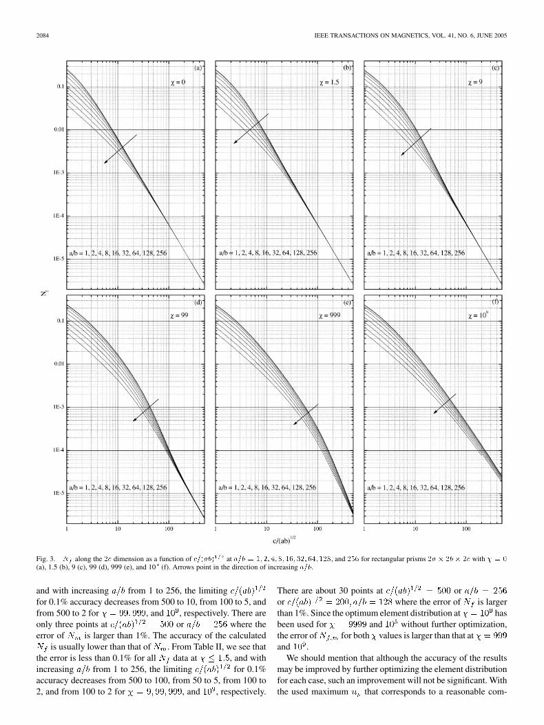
Fig. 3. N along the 2c dimension as a function of c=(ab) at a=b = 1; 2; 4; 8; 16; 32;64;128, and 256 for rectangular prisms 2a� 2b� 2c with � = 0(a), 1.5 (b), 9 (c), 99 (d), 999 (e), and 10 (f). Arrows point in the direction of increasing a=b.

and with increasing from 1 to 256, the limitingfor 0.1% accuracy decreases from 500 to 10, from 100 to 5, andfrom 500 to 2 for , and , respectively. There areonly three points at or where theerror of is larger than 1%. The accuracy of the calculated

is usually lower than that of . From Table II, we see thatthe error is less than 0.1% for all data at , and withincreasing from 1 to 256, the limiting for 0.1%accuracy decreases from 500 to 100, from 50 to 5, from 100 to2, and from 100 to 2 for , and , respectively.

There are about 30 points at oror where the error of is largerthan 1%. Since the optimum element distribution at hasbeen used for and without further optimization,the error of for both values is larger than that atand .

We should mention that although the accuracy of the resultsmay be improved by further optimizing the element distributionfor each case, such an improvement will not be significant. Withthe used maximum that corresponds to a reasonable com-

CHEN et al.: DEMAGNETIZING FACTORS FOR RECTANGULAR PRISMS 2085

Fig. 4. Comparison of N and N versus c=(ab) curves at � = 10 withdemagnetizing factor N of ellipsoids of semi-axes a; b, and c for a=b = 1; 32,and 128 in (a), (b), and (c), respectively.

putation time, we cannot calculate forwith an accuracy better than 1%. A further improvement in theaccuracy would require a higher and a greatly increased com-putation speed. The present high accuracy in a wide parameterregion has been realized following all the points described inSection II after our long-term development, and we believe thatfurther developments should still be proceeded in a heuristicway. Numerical calculation has been widely used in magneto-statics problems, and we feel that the calculation of forsimple geometries can be a good test for treating complex sys-tems, since the correctness and accuracy of the results can bewell estimated for simple cases but not for the complex ones.

C. for Arbitrary Aspect Ratios

The results of numerical calculations can only give discretedata points. Since accurate require a huge computationtime, such data points should be reduced to a minimum number.

As functions of , and , the number and distribu-tion of the calculated points should ensure that accuratecurves of versus , and be obtained fromthem. Plotting figures, we always connect a set of functionaldata points by a spline line in this paper. As explained earlier,with the chosen values, curves canbe plotted accurately in log–log scales for each pair of and

. After studying the conjugate relations in two-dimensionalcase [10], we know that versus the permeability

is a log–log smooth function, so that a choice ofis reasonable. We have added one point at

, with which for weak magnetic materials can be ob-tained more accurately. The value of is chosen in geometricprogression growth of common factor 2, and we see from Figs. 2and 3 that curves are quite uniformly placed whenis large, whereas they become denser when . In fact,

and are physically identical, and is aparabolic curve centered at , which can be drawn ac-curately with the chosen values of . Thus, with datalisted in Tables I and II, for any intermediate values of

, and can be obtained by interpolation with asatisfactory accuracy, and may also be obtained with lessaccuracy by extrapolation if their values are beyond the calcu-lated range.

In actual magnetic measurements, the sample dimensions arefixed and one needs to get at given values ofand . As examples, we assume arbitrarily two samples tohave and with a common . Allthese values are not included in Tables I and II. The interpolationof is performed as follows.

We first draw spline curves in log–log scalesfor , and and , and usingdata given in Table I, as demonstrated in Fig. 5(a)–(c). In order toget accurate spline curves, four values around 7.5 areused. Drawing a vertical line at , we obtain the

coordinate of its intersection point with eachcurve, so that at and every pair ofand is obtained. We next draw spline curve for each

value and , as shown in Fig. 5(d)–(f). Notethat data points for , and are addedwhen plotting spline curves, so that smooth symmetric paraboliccurves are obtained. Drawing vertical lines at and

, we obtain data by reading the coordinate of theintersection points. These data points are connected by spline

versus curves in Fig. 6, where they are comparedwith two nearby curves directly drawn using accurate data inTable I. Note that in Fig. 6, the scale is set linear rather thanlogarithmic for ease of reading.

In the above cases all the directly calculated data points haveerror less than 0.1%, and the interpolated curves have added anerror about 0.2%, as checked by extra direct calculations (seeTable III).

D. Exemplified Application

The calculated versus , and have var-ious applications [3]. We introduce one that is a good represen-

2086 IEEE TRANSACTIONS ON MAGNETICS, VOL. 41, NO. 6, JUNE 2005

Fig. 5. Spline N versus c=(ab) curves for a=b = 1; 2; 4; 8, and 16 and � = 0 (a), 9 (b), and 999 (c) connecting data points obtained from Table I. SplineN versus a=b curves for c=(ab) = 7:5 and � = 0 and 1:5 (d), 9 and 99 (e), and 999 (f). Arrows point in the direction of increasing a=b.

tative of the classical model of constant and requires very ac-curate data.

It is known that for a ferromagnet at temperatures slightlyabove the Curie temperature, , the temperature dependentsusceptibility follows:

(13)

where and are constants and the latter is referred to as thecritical exponent. The value of has been calculated using dif-ferent models of magnetic structure. For example, it equals 1,1.241, and 1.386 for the mean field, three-dimensional Ising, andthree-dimensional Heisenberg models, respectively [15]. Using(13), we can determine precisely and from measured

. The problem is that in the magnetometric measurements,

the directly measured susceptibility is and ithas to be corrected to using

(14)

In the past, such a correction was made assuming to beconstant, determined by the maximum in its field or de-pendence [15]. According to (14), such determined cor-responds to its value at a certain high only, and it cannotbe properly used for the correction since (13) involves thatchanges usually by two or three orders of magnitude.

To make a proper demagnetizing correction for the exempli-fied samples whose functions are shown in Fig. 6,and may be obtained iteratively. We expect that such a correc-tion should give the value of different from that using the tra-ditional way, so that the physical conclusion might be changed

CHEN et al.: DEMAGNETIZING FACTORS FOR RECTANGULAR PRISMS 2087

Fig. 6. Interpolated spline N versus �+1 curves for c=(ab) = 7:5 anda=b = 1:5 (a) and 6 (b) (solid lines). The dashed and dotted lines show accuratenearby curves drawn directly from data listed in Table I.

concerning the magnetic structure. The correction is performedusing

(15)

where the superscripts denote the iteration step.When , we set to get using the interpo-lated curves in Fig. 6 and so using (15). We thenuse to get and so and use to get andso in a similar way. Assuming , andfor sample 1 with and , and forsample 2 with , the results are listed in Table III.

We see from Table III that both and become quitestable when , and therefore, three times of iterations arealready enough and the final results can be taken as

and , as listed in Table III.Moreover, we have both and to in-crease with increasing . It is important to make an error anal-ysis as follows.

Assuming the relative error of the measured and the cal-culated is and , respectively, the relative error inthe final calculated from (14) will be estimated by

(16)

if both partial errors are independent to each other. We see from(16) that is greater than at least by a factor , andthe error in gives an additional contribution to the error of

if is large. Assuming % and %

will increase from 1.1% to 9% with increasing for thetwo samples in Table III. Thus, we conclude that in order to get

with a reasonable accuracy, and should be veryaccurate and should be so large that is not toolarge.

V. CONCLUSION

For rectangular prisms of dimensions with con-stant material susceptibility , we have calculated their flux-metric and magnetometric demagnetizing factors alongthe axis as functions of the values of and aspect ratios

and . The results are listed in Tables I and II with620 points in a parameter region of

, and . The error of is less than 1% formore than 95% of points, and it decreases to less than 0.01%with decreasing , and . Since the distributionof the calculation points is well designed, for any valuesof parameters in the calculated region may be conveniently ob-tained by interpolations using spline lines with an satisfactoryadditional error of about 0.2%. Our results can be very usefulfor high quality magnetic measurements and accurate quantita-tive studies of magnetic materials.

APPENDIX

SUMMARY OF QUANTITIES USED IN THE PAPER

The studied body is a rectangular prism with a constant ma-terial susceptibility [or constant material permeability

] centered at the origin and having dimensions ,and along the , and axes, respectively, in a uniform ap-plied magnetic field in the direction.

Magnetic field being the demagnetizingfield produced by magnetic poles in the prism and magnetization

. Because the magnetic flux densityand , we have in the

prism, so that magnetic poles are present on the surface only andare characterized by surface magnetic pole density ,where is the outward unit vector normal to the surface.

Since and are generally nonuniform, we use andto stand for their average in general. is the compo-

nent of . and are the component ofand when the average is made over the midplane.

and are the component of and whenthe average is made over the entire volume. Since these averagequantities are generally used for both the ideal correct valuesand calculated values with some error, we redefineand to be the ideal correct values when both typesof values appear in (12). and are the midplane av-erage and volume average of the component of the per unit

generated by the th element in the region of .is demagnetizing factor for ellipsoid along a principal

axis. is average demagnetizing factor in general. isfluxmetric demagnetizing factor, i.e., and when the averageis made over the midplane. is magnetometric demagne-tizing factor, i.e., and when the average is made overthe entire volume. are calculated using “surfacemethod” through . are calculated using

2088 IEEE TRANSACTIONS ON MAGNETICS, VOL. 41, NO. 6, JUNE 2005

TABLE IIIDETERMINATION OF N AND � FROM THE MEASURED SAMPLE DIMENSIONS AND � . DIRECTLY CALCULATED N ARE WRITTEN WITHIN PARENTHESES

“volume method” through . are correctedusing (11) from and .

is external susceptibility., and are used for the center coordinates of the th

element; in the region of , these coordinates are, or . , and are element

size along the , and axes, respectively. , andare the increments used for calculating element divisions

along the , and axes, respectively, from (3)–(5). ,and are the division numbers along the , and axes,respectively. . is the total elementnumber.

, and are the relative error in , and ,respectively.

ACKNOWLEDGMENT

This work was supported by Spanish Ministerio de Edu-cación y Ciencia Project Number FIS2004-02792, CatalanProjects SGR2001-00189, and CeRMAE. E. Pardo acknowl-edges the support of DURSI from the Generalitat de Catalunya.The authors thank the reviewers for their interest in the paperand valuable suggestions for its improvement.

REFERENCES

[1] R. M. Bozorth, Ferromagnetism, New York: Wiley, 2003, pp. 843–861.[2] D.-X. Chen, Physical Bases of Magnetic Measurements. Beijing,

China: China Mechanical Industry, 1985, pp. 175–206.

[3] D.-X. Chen, J. A. Brug, and R. B. Goldfarb, “Demagnetizing factors forcylinders,” IEEE Trans. Magn., vol. 27, no. 4, pp. 3601–3619, Jul. 1991.

[4] J. A. Osborn, “Demagnetizing factors of the general ellipsoid,” Phys.Rev., vol. 67, pp. 351–357, Jun. 1945.

[5] P. Rhodes and G. Rowlands, “Demagnetising energies of uniformlymagnetized rectangular blocks,” in Proc. Leeds Phil. Lit. Soc., vol. 6,1954, pp. 191–210.

[6] R. I. Joseph, “Ballistic demagnetizing factor in uniformly magnetizedrectangular prisms,” J. Appl. Phys., vol. 38, pp. 2405–2406, 1967.

[7] D.-X. Chen, E. Pardo, and A. Sanchez, “Demagnetizing factors of rect-angular prisms and ellipsoids,” IEEE Trans. Magn., vol. 38, no. 4, pp.1742–1752, Jul. 2002.

[8] W. F. Brown, Jr., Magnetostatic Principles in Ferromagnetism. Ams-terdam, The Netherlands: North-Holland, 1962, pp. 187–192.

[9] D.-X. Chen, C. Prados, E. Pardo, A. Sanchez, and A. Hernando, “Trans-verse demagnetizing factors of long rectangular bars: I. Analytical ex-pressions for extreme values of susceptibility,” J. Appl. Phys., vol. 91,pp. 5254–5259, Apr. 2002.

[10] E. Pardo, A. Sanchez, and D.-X. Chen, “Transverse demagnetizing fac-tors of long rectangular bars: II. Numerical calculations for arbitrary sus-ceptibility,” J. Appl. Phys., vol. 91, pp. 5260–5267, Apr. 2002.

[11] E. Pardo, D.-X. Chen, and A. Sanchez, “Demagnetizing factors of squarebars,” IEEE Trans. Magn., vol. 40, no. 3, pp. 1491–1499, May 2004.

[12] , “Demagnetizing factors for completely shielded rectangularprisms,” J. Appl. Phys., vol. 96, pp. 5365–5369, Nov. 2004.

[13] T. L. Templeton and A. S. Arrott, “Magnetostatics of rods and bars ofideally soft ferromagnetic materials,” IEEE Trans. Magn., vol. 23, no. 5,pp. 2650–2652, Sep. 1987.

[14] W. H. Press et al., Numerical Recipes in C. Cambridge, U.K.: Cam-bridge Univ. Press, 1992.

[15] M. Seeger, S. N. Kaul, H. Kronmuller, and R. Reisser, “Asymptoticcritical behavior of Ni,” Phys. Rev. B, Condens. Matter, vol. 51, pp.12 585–12594, 1995.

Manuscript received October 26, 2004; revised February 28, 2005.