geosciences

Article

Elastic Settlement Analysis of Rigid RectangularFootings on Sands and Clays

Lysandros Pantelidis 1,* and Elias Gravanis 1,2

1 Department of Civil Engineering and Geomatics, Cyprus University of Technology, Limassol 3036, Cyprus;elias.gravanis@cut.ac.cy

2 Eratosthenes Centre of Excellence, Cyprus University of Technology, P.O. Box 50329, Limassol 3603, Cyprus* Correspondence: lysandros.pantelidis@cut.ac.cy; Tel.: +357-2500-2271

Received: 16 November 2020; Accepted: 30 November 2020; Published: 4 December 2020 �����������������

Abstract: In this paper an elastic settlement analysis method for rigid rectangular footings applicableto both clays and sands is proposed. The proposed method is based on the concept of equivalent shape,where any rectangular footing is suitably replaced by a footing of elliptical shape; the conditionsof equal area and equal perimeter are satisfied simultaneously. The case of clay is differentiatedfrom the case of sand using different contact pressure distribution, whilst, additionally, for the sands,the modulus of elasticity increases linearly with depth. The method can conveniently be calibratedagainst any set of settlement data obtained analytically, experimentally, or numerically; in thisrespect the authors used values which have been derived analytically from third parties. Among themost interesting findings is that sands produce “settlement x soil modulus/applied pressure” valuesapproximately 10% greater than the respective ones corresponding to clays. Moreover, for largePoisson’s ratio (v) values, the settlement of rigid footings is closer to the settlement correspondingto the corner of the respective flexible footings. As v decreases, the derived settlement of the rigidfooting approaches the settlement value corresponding to the characteristic point of the respectiveflexible footing. Finally, corrections for the net applied pressure, footing rigidity, and non-elasticresponse of soil under loading are also proposed.

Keywords: elastic settlement; shallow foundations; rigid footings; contact pressure; equivalent shape

1. Introduction

The problem of settlement of shallow foundations is among the more important ones in classicalsoil mechanics. During the last several decades a great number of approaches has been proposed in theliterature for the title problem, an exact solution of which is still not available. In this respect, solutionshave been provided by various authors [1–11]. Numerical results for perfectly smooth, uniformlyloaded rectangular rafts, of any rigidity resting on a homogeneous elastic layer which is underlainby a rough rigid base, were presented in graphical form by Fraser and Wardle [12]. Semi-empiricalapproaches combining the theory of elasticity with experimental and/or numerical results also exist inthe literature [13–17]. Schiffman and Aggarwala [18] and Mayne and Poulos [15] used the concept ofequivalent ellipse and circle respectively (equivalency as for the footprint area).

In this paper an elastic settlement analysis method for rigid rectangular footings applicable to bothclays and sands is proposed. The proposed method is based on the concept of equivalent shape, whereany rectangular B× L footing is suitably replaced by a footing of elliptical shape. The suitability of theequivalent shape concept is deeply investigated aiming at the production of analytical expressions forthe elastic settlement analysis of rigid rectangular footings on sands and clays. As shown, this conceptis only valid when the equivalent shape satisfies both the condition of equal area and equal perimeterlength at the same time. The case of clay is differentiated from the case of sand using different contact

Geosciences 2020, 10, 491; doi:10.3390/geosciences10120491 www.mdpi.com/journal/geosciences

Geosciences 2020, 10, 491 2 of 18

pressure distribution, whilst the modulus of elasticity for the case of sands additionally increaseslinearly with depth.

2. Settlement of Rigid Elliptical Footing

Boussinesq [19] solved the problem of stresses produced at any point in a homogenous, elastic,isotropic, and semi-infinite medium as the result of a point load applied on the surface. Following thenotation of Figure 1, the increase in normal stresses caused by the point load P is

∆σx =P

2π

(3x2zL5 −

(1− 2ν)(

x2− y2

Lr2(L + z)+

y2zL3r2

)), (1)

∆σy =P

2π

(3y2zL5 −

(1− 2ν)(

y2− x2

Lr2(L + z)+

x2zL3r2

)), (2)

∆σz =3P2π

z3

L5 , (3)

where L =√

x2 + y2 + z2, r =√

x2 + y2 and ν is the Poisson’s ratio (see [20–22]).

Geosciences 2020, 10, x FOR PEER REVIEW 2 of 19

analytical expressions for the elastic settlement analysis of rigid rectangular footings on sands and

clays. As shown, this concept is only valid when the equivalent shape satisfies both the condition of

equal area and equal perimeter length at the same time. The case of clay is differentiated from the

case of sand using different contact pressure distribution, whilst the modulus of elasticity for the case

of sands additionally increases linearly with depth.

2. Settlement of Rigid Elliptical Footing

Boussinesq [19] solved the problem of stresses produced at any point in a homogenous, elastic,

isotropic, and semi-infinite medium as the result of a point load applied on the surface. Following

the notation of Figure 1, the increase in normal stresses caused by the point load P is

2 2 2 2

5 2 3 2

31 2

2x

P x z x y y z

L Lr L z L r

,

(1)

2 2 2 2

5 2 3 2

31 2

2y

P y z y x x z

L Lr L z L r

, (2)

3

5

3

2z

P z

L

, (3)

where 2 2 2L x y z , 2 2r x y and ν is the Poisson’s ratio (see [20–22]).

Figure 1. Stresses in an elastic medium caused by a point load acting on the surface of a semi-infinite

mass [23].

The above equations along with the equation effectively representing the contact pressure

distribution leads to the elastic settlement of footing following a standard procedure (see [19,24]). In

this respect, by using the following contact pressure distribution (see [18]):

.

2 2

2 2

1

2 1

ellPp

ab x y

a b

, (4)

The settlement of a rigid elliptical footing can be obtained in a way similar to the case of

Boussinesq’s [19] rigid circular footing (see also [24]); where .ellP is the total load on the elliptical

rigid footing (the origin of the axes lies on the centroid of the elliptical disc), whilst a and b are the

two radii defining the ellipse.

The infinitesimal point load P at any point (x,y) inside the ellipse is, thus, given by

2 2

2 22 1

qP pdxdy dxdy

x y

a b

, (5)

where

Figure 1. Stresses in an elastic medium caused by a point load acting on the surface of a semi-infinitemass [23].

The above equations along with the equation effectively representing the contact pressuredistribution leads to the elastic settlement of footing following a standard procedure (see [19,24]).In this respect, by using the following contact pressure distribution (see [18]):

p =Pell.πab

1

2√

1− x2

a2 −y2

b2

. (4)

The settlement of a rigid elliptical footing can be obtained in a way similar to the case ofBoussinesq’s [19] rigid circular footing (see also [24]); where Pell. is the total load on the elliptical rigidfooting (the origin of the axes lies on the centroid of the elliptical disc), whilst a and b are the two radiidefining the ellipse.

The infinitesimal point load P at any point (x,y) inside the ellipse is, thus, given by

P = pdxdy =q

2√

1− x2

a2 −y2

b2

dxdy, (5)

whereq =

Pell.πab

, (6)

is the load per unit area of the footing.

Geosciences 2020, 10, 491 3 of 18

Hence, the increase in the normal stress in the i-axis due to loading over the elliptical surface areacan be found by integrating the respective stress increase ∆σi (i = x, y or z) (see Equations (1)–(3)) overthis area using Equation (5). That is:

∆σi,Ell. =x

ellipse

∆σi(x, y, z). (7)

Note that the differentials dx and dy are included in P (see Equation (5)). The integration canconveniently be done by changing to polar variables r and θ, setting x = ar cosθ and y = br sinθ,where the ranges of the radial and angular variables, respectively, are 0 ≤ r ≤ 1 and 0 ≤ θ ≤ 2π. For thearea element in the polar variables then it stands that dxdy = abrdrdθ.

The unit vertical strain is, then, calculated from the constitutive relationship of Hooke’s Law:

εz =1E

[∆σz,Ell. − ν

(∆σx,Ell. + ∆σy,Ell.

)](8)

and finally, the footing settlement, ρr, corresponding to a layer of thickness H is

ρr =

H∫z = 0

εzdz =qbEβ, (9)

where

β =1b

H∫z = 0

Izdz =

H/b∫ζ = 0

(1 + v)(1− 2ν) + 2(1− ν2)(1 + k2)ζ2 + (1 + v)(3− 2ν)k2ζ4

2(1 + ζ2)3/2(1 + k2ζ2)3/2dζ, (10)

with ζ = z/b and k = b/a; Iz is the strain influence factor. The integration as for z can easily beimplemented numerically in spreadsheet so that the effect of varying soil modulus with depth to betaken into account in a way similar to Schmertmann’s method [14].

In the case of homogenous semi-infinite mass, the settlement becomes:

ρr =qbE

kK(e)(1− ν2

), (11)

where e =√

1− k2 is the eccentricity of the ellipse and K(x) is the complete elliptic integral of thefirst kind [25]. Due to the fact that in the circular case K(0) = π/2 (because e = 0 and also, k = 1),Equation (11) goes over to the well-known expression of Boussinesq [19,24]:

ρr =πqa2E

(1− ν2). (12)

3. Elastic Settlement of the Equivalent B× L Rectangular Footing

From the theory of elasticity for flexible footings over semi-infinite media, it is well known thatthe settlement at the center of a uniformly loaded square footing having edge B is approximately equalto the respective settlement of a circular footing of equal area (radius of footing equal to B/

√π) [26];

the percentage difference in settlement between these two special cases is only 0.53%.The concept of shape equivalency has been used in the past by Mayne and Poulos [15], where any

B × L rectangular footing is reduced to a circular footing of equal area. The radius of Mayne andPoulos’ [15] equivalent circle is

aeq =√

BL/π. (13)

Geosciences 2020, 10, 491 4 of 18

Several years earlier, Schiffman and Aggarwala [18] suggested that the two radii defining theequivalent elliptical footing of a B× L rectangular footing be

a = L/√π

b = B/√π

}with a ≥ b. (14)

Schiffman and Aggarwala [18] considered the problem of an elastic half-space loaded on thesurface by a rigid elliptical footing. They developed general formulae for the stresses and displacementswithin and on the surface of the solid. It is noted that Equation (14) derives from the condition of equalarea and from B/L = b/a = k; the condition of equal perimeter is not satisfied.

Sovinc [8] worked analytically on the problem of settlement of smooth, rectangular footing restingon the surface of a finite layer with ν = 0.5, providing a “calibration platform” for the proposed method.He expressed the settlement of footing with respect of the long footing dimension, L, as follows:

ρr =qLEβ. (15)

Unfortunately, Sovinc published β vs. H/L curves and not a closed-form expression for β;for readers’ convenience, these curves can be found in the freely available book of Poulos and Davis [27](www.usucger.org/PandD/complete_book.pdf). Sovinc’s [8] values were compared by the authorsagainst the respective values given by Butterfield and Banerjee ([10]; also in Poulos and Davis [27])providing, in turn, the necessary validation of the “calibration platform” mentioned above. The resultsof these studies are in full agreement.

From the β vs. H/L comparison chart of Figure 2 it is clear that Schiffman and Aggarwala’s [18]equivalent shape (see Equation (14)) is not a reliable choice.

Geosciences 2020, 10, x FOR PEER REVIEW 4 of 19

a L

b B

with a b . (14)

Schiffman and Aggarwala [18] considered the problem of an elastic half-space loaded on the

surface by a rigid elliptical footing. They developed general formulae for the stresses and

displacements within and on the surface of the solid. It is noted that Equation (14) derives from the

condition of equal area and from B L b a k ; the condition of equal perimeter is not satisfied.

Sovinc [8] worked analytically on the problem of settlement of smooth, rectangular footing

resting on the surface of a finite layer with ν = 0.5, providing a “calibration platform” for the proposed

method. He expressed the settlement of footing with respect of the long footing dimension, L , as

follows:

r

qL

E . (15)

Unfortunately, Sovinc published vs. H L curves and not a closed-form expression for ; for

readers’ convenience, these curves can be found in the freely available book of Poulos and Davis [27]

(www.usucger.org/PandD/complete_book.pdf). Sovinc’s [8] values were compared by the authors

against the respective values given by Butterfield and Banerjee ([10]; also in Poulos and Davis [27])

providing, in turn, the necessary validation of the “calibration platform” mentioned above. The

results of these studies are in full agreement.

From the vs. H L comparison chart of Figure 2 it is clear that Schiffman and Aggarwala’s

[18] equivalent shape (see Equation (14)) is not a reliable choice.

Figure 2. Comparison chart between Sovinc’s [8] factor for rigid rectangular footing (ν = 0.5) and

the respective one based on Schiffman and Aggarwala ([18]; denoted as S&A on the figure) equivalent

ellipse.

The authors also considered the case of equivalent ellipse satisfying both the condition of area

and perimeter. The area of the ellipse is exact and given by the expression ab . The perimeter is

exactly given by 2 ( )aE e , where ( )E x is the complete elliptic integral of second kind [25]. This is a

transcendental expression which can be calculated explicitly through infinite series. Instead, one may

use Ramanujan’s approximate formula giving values very close to the exact perimeter values:

3 3 3a b a b a b . (16)

The two radii of the equivalent ellipse are then:

Figure 2. Comparison chart between Sovinc’s [8] β factor for rigid rectangular footing (ν = 0.5)and the respective one based on Schiffman and Aggarwala ([18]; denoted as S&A on the figure)equivalent ellipse.

The authors also considered the case of equivalent ellipse satisfying both the condition of areaand perimeter. The area of the ellipse is exact and given by the expression πab. The perimeter isexactly given by 2aE(e), where E(x) is the complete elliptic integral of second kind [25]. This is atranscendental expression which can be calculated explicitly through infinite series. Instead, one mayuse Ramanujan’s approximate formula giving values very close to the exact perimeter values:

Π ≈ π(3(a + b) −

√(3a + b)(a + 3b)

). (16)

Geosciences 2020, 10, 491 5 of 18

The two radii of the equivalent ellipse are then:

a = 12π

(B + L + 1

3

(η−√

6√(B + L)(η+ 2(B + L)) − 5πBL

))b = BL

aπ

, (17)

with η =

√3(B + L)2 + 2πBL.

The new equivalent shape gave β vs. H/L curves close to those given by Sovinc indicating theneed for calibration with respect of the footing shape. The new βR factor referring to the equivalentrectangular footing is a function of the aspect ratio of footing, L/B. The calibration against Sovinc’s [8]chart gave:

βR = Is · β(ζR), (18)

whereIs = 2

(1 + log

LB

)Bo

L, (19)

and Bo = 1 m (unit width). The notation β(ζR) denotes the use of Equation (10) but replacing ζ with

ζR =(0.85λ+

zb

) λ0.85

, λ = min{(

1 + logLB

)1/3− 0.05, 1.1

}. (20)

The expression for the settlement, thus, becomes

ρr =qLEβR, (21)

or, in the more familiar form,

ρr =qBE

IHIs1(1− ν2

), (22)

with

IH =Bo

B

H/b∫ζ = 0

1 + 2(1 + k2)ζ2R(1− v) − 2v + k2ζ4

R(3− 2ν)

2((1 + ζ2

R)(1 + k2ζ2R)

)3/2(1− v)

dζ, (23)

andIs1 = 2

(1 + log

LB

). (24)

The integral in Equation (23) requires numerical evaluation, which can be easily done using oneof the numerous proprietary and non-proprietary mathematical programs available.

As shown is Figure 3, the new βR factor compares very well with Sovinc’s β factor. Although,the proposed method was calibrated manually against Sovinc’s [8] dimensionless values, any set ofrelevant data could be used instead, while the procedure could be facilitated by the use of a statisticalanalysis program. The use of elastic settlement values derived from 3D finite element analysis issubject matter of work by the authors.

It is interesting that, Equations (19) and (20) contain the term (1 + log(L/B)), best known fromthe influence depth of footings proposed by Terzaghi et al. [28], i.e., zl = 2B(1 + log(L/B))

The effect of footing shape on the modulus of elasticity has not yet been considered in the analysis.In this respect, Terzaghi et al. [28] suggested that

EEaxis.

=(1 + 0.4 log

LB

), (25)

Geosciences 2020, 10, 491 6 of 18

with 1≤ L/B ≤ 10, where, Eaxis. the triaxial modulus of elasticity of soil. For 1≤ L/B ≤ 10, the E/Eaxis.

ratio ranges between 1 and 1.4 for the axisymmetric and plane strain condition, respectively. Veryrecently, Pantelidis [29,30] showed that the correct relationship is

EEaxis.

=(1 + log

LB

). (26)

Thus, including the effect of footing shape on the modulus of soil, the footing settlement will be

ρr =2qB

Eaxis.IH

(1− ν2

)or

2qBo

Eaxis.β(ζR). (27)

The triaxial modulus of soil, Eaxis., can be obtained by the triaxial compression test or continuousprobing tests.Geosciences 2020, 10, x FOR PEER REVIEW 6 of 19

Figure 3. Comparison chart between Sovinc’s [8] factor for rigid rectangular footing and the

proposed R ; all curves refer to ν = 0.5.

The effect of footing shape on the modulus of elasticity has not yet been considered in the

analysis. In this respect, Terzaghi et al. [28] suggested that

.

1 0.4logaxis

E L

E B

, (25)

with 1 10L B , where, .axisE the triaxial modulus of elasticity of soil. For 1 10L B , the

.axisE E

ratio ranges between 1 and 1.4 for the axisymmetric and plane strain condition, respectively. Very

recently, Pantelidis [29,30] showed that the correct relationship is

axis.

1 logE L

E B

. (26)

Thus, including the effect of footing shape on the modulus of soil, the footing settlement will be

2

axis. axis.

221 or o

r H R

qBqBI

E E , (27)

The triaxial modulus of soil, axis.E , can be obtained by the triaxial compression test or continuous

probing tests.

4. Elastic Settlement Analysis of Rigid Footings on Sands

The above formulations were based on the contact pressure distribution of Equation (4). This

contact pressure of parabolic form, where the minimum and the maximum pressure value is found

at the center and the edges of footing respectively (Figure 4a), is, however, more suitable for clays.

For smooth rigid footings on clean sand, the minimum and maximum contact pressure are observed

at the edges and the center of the footing respectively, as shown in Figure 4b [28,31].

Figure 3. Comparison chart between Sovinc’s [8] β factor for rigid rectangular footing and the proposedβR; all curves refer to ν = 0.5.

4. Elastic Settlement Analysis of Rigid Footings on Sands

The above formulations were based on the contact pressure distribution of Equation (4).This contact pressure of parabolic form, where the minimum and the maximum pressure valueis found at the center and the edges of footing respectively (Figure 4a), is, however, more suitablefor clays. For smooth rigid footings on clean sand, the minimum and maximum contact pressure areobserved at the edges and the center of the footing respectively, as shown in Figure 4b [28,31].

Referring to an elliptical rigid footing over sand, the contact pressure distribution can beeffectively represented by a half spheroid attached under the footing. The infinitesimal point load P inEquations (1)–(3) can, then, be expressed as follows:

P =32

q

√1−

x2

a2 −y2

b2 dxdy. (28)

In addition, as known sands are compacted under their own weight, where their modulus ofelasticity usually appears to increase linearly with depth obeying Gibson’s law [32]:

E(z) = Eo + kEz, (29)

where Eo = the soil modulus directly beneath the foundation base (z = 0), kE = the rate of increase ofmodulus with depth (units of E per unit depth) and z = the depth having modulus E(z). This has also

Geosciences 2020, 10, 491 7 of 18

been proved experimentally by the first author [29] performing a series of Dynamic Probing Light(DPL) tests on clean quarry sand. Indeed, this phenomenon occurs immediately after deposition and itis due to the increase of the density caused by the overburden mass in combination with the increasedconfinement at greater depths. In a similar manner, any surcharge on the surface of the sand materialwill have an analogous impact. In this respect, it was suggested [29] that

E(z) = Eo + kEσz

γ= Eo + kE

(z +

qγ

Iσ

)= Eo

[1 +

kE

Eo

(z +

qγ

Iσ

)], (30)

where γ is the unit weight of soil, σz = γz + qIσ and Iσ is the well-known stress influence factor; Iσvalues for various footing shapes can be found in any soil mechanics book (e.g., [26]). Therefore,the settlement is given as follows:

ρr =qLEoβR =

qLEo

Isβ(ζR). (31)

The factor β(ζR) is calculated using the following Equation (recall Equation (10))

β =1b

H∫z = 0

Iz(z)1 + kE(z + qIσ/γ)/Eo

dz =

H/b∫ζ = 0

Iz(ζ)

1 + kEb(ζ+ qIσ/(bγ))/Eodζ, (32)

with

Iz(ζ) = (ν+ 1)

3

2√(1 + ζ2)(1 + k2ζ2)

− νF4

, (33)

and

F4 = 3−3k2ζ2π

∫ 2π

0

cot−1(

kζ√

1−(1−k2) sin2 θ

)(1− (1− k2) sin2 θ)

3/2dθ, (34)

whilst ζmust again be replaced by ζR (recall Equation (20)) as indicated in Equation (31). It is remindedthat Is is given by Equation (19). The integral of Equation (34) has been transformed to polar variableswith x = ar cosθ and y = br sinθ for the sake of convenience. Unfortunately, the integral inEquation (34) requires numerical evaluation. For avoiding such a procedure, the F4 term is given inchart form in Figure 5.Geosciences 2020, 10, x FOR PEER REVIEW 7 of 19

Figure 4. Assumed contact pressure distribution of smooth rigid footing on (a) cohesive soil and (b)

cohesionless soil.

Referring to an elliptical rigid footing over sand, the contact pressure distribution can be

effectively represented by a half spheroid attached under the footing. The infinitesimal point load P

in Equations (1)–(3) can, then, be expressed as follows:

2 2

2 2

31

2

x yP q dxdy

a b , (28)

In addition, as known sands are compacted under their own weight, where their modulus of

elasticity usually appears to increase linearly with depth obeying Gibson’s law [32]:

( ) o EE z E k z , (29)

where oE = the soil modulus directly beneath the foundation base (z = 0), Ek = the rate of increase of

modulus with depth (units of E per unit depth) and z = the depth having modulus ( )E z . This has

also been proved experimentally by the first author [29] performing a series of Dynamic Probing

Light (DPL) tests on clean quarry sand. Indeed, this phenomenon occurs immediately after

deposition and it is due to the increase of the density caused by the overburden mass in combination

with the increased confinement at greater depths. In a similar manner, any surcharge on the surface

of the sand material will have an analogous impact. In this respect, it was suggested [29] that

( ) 1z E

o E o E o

o

kq qE z E k E k z I E z I

E

, (30)

where γ is the unit weight of soil, σz = γz + qIσ and Iσ is the well-known stress influence factor; Iσ values

for various footing shapes can be found in any soil mechanics book (e.g., [26]). Therefore, the

settlement is given as follows:

r R s R

o o

qL qLI

E E . (31)

The factor R is calculated using the following equation (recall Equation (10))

0 0

( ) ( )1

1 1 ( )

H bH

z z

E o E oz

I z Idz d

b k z qI E k b qI b E

, (32)

with

42 2 2

3( ) ( 1)

2 (1 )(1 )zI F

k

, (33)

and

Figure 4. Assumed contact pressure distribution of smooth rigid footing on (a) cohesive soil and (b)cohesionless soil.

It is finally mentioned that, for the special case of H→∞ and kE = 0 the factor β can be obtainedfully analytically (see Appendix A).

Geosciences 2020, 10, 491 8 of 18

Geosciences 2020, 10, x FOR PEER REVIEW 8 of 19

1

2 222

4 2 2 3/20

cot1 (1 )sin3

32 (1 (1 )sin )

k

kkF d

k

,

(34)

whilst ζ must again be replaced by ζR (recall Equation (20)) as indicated in Equation (31). It is

reminded that sI is given by Equation (19). The integral of Equation (34) has been transformed to

polar variables with cosx ar and siny br for the sake of convenience. Unfortunately, the

integral in Equation (34) requires numerical evaluation. For avoiding such a procedure, the 4F term

is given in chart form in Figure 5.

It is finally mentioned that, for the special case of H and kE = 0 the factor can be

obtained fully analytically (see Appendix A).

Figure 5. Chart giving the 4F factor with respect to .

5. Other Factors Affecting Elastic Settlement of Shallow Foundations

The modulus of elasticity and in turn, the elastic settlement of shallow foundations may

seriously be affected by various factors, such as the shape of the footing [29,30,33], the footing load

(phenomenon occurring in sands; [29]), the embedment depth of footing [15,34–38], and a possible

water table rise into the influence depth of footing [39–48]. Creep in sands may also affect the

settlement of shallow foundations (see [13,28]). The rigidity of footing, the net applied pressure and

the non-elastic response of the ground are also factors affecting settlement of shallow foundations for

which corrections are suggested below.

5.1. Correction for Footing Rigidity

According to ACI Committee 336, DIN 4018 and IS 2950-1 [49–51], whether a foundation behaves

as a rigid or a flexible structure depends on the relative stiffness of the structure and the foundation

soil. The relative stiffness factor, rK , is given as follows:

3

b

r

E IK

EL B , (35)

where bE I is the flexural rigidity of the superstructure and foundation per unit length at right

angles to B and bE is the modulus of concrete. An approximate value of

bE I per unit width of

Figure 5. Chart giving the F4 factor with respect to ζ.

5. Other Factors Affecting Elastic Settlement of Shallow Foundations

The modulus of elasticity and in turn, the elastic settlement of shallow foundations may seriouslybe affected by various factors, such as the shape of the footing [29,30,33], the footing load (phenomenonoccurring in sands; [29]), the embedment depth of footing [15,34–38], and a possible water table riseinto the influence depth of footing [39–48]. Creep in sands may also affect the settlement of shallowfoundations (see [13,28]). The rigidity of footing, the net applied pressure and the non-elastic responseof the ground are also factors affecting settlement of shallow foundations for which corrections aresuggested below.

5.1. Correction for Footing Rigidity

According to ACI Committee 336, DIN 4018 and IS 2950-1 [49–51], whether a foundation behavesas a rigid or a flexible structure depends on the relative stiffness of the structure and the foundationsoil. The relative stiffness factor, Kr, is given as follows:

Kr =EbI

EL3B, (35)

where EbI is the flexural rigidity of the superstructure and foundation per unit length at right angles toB and Eb is the modulus of concrete. An approximate value of EbI per unit width of building can bedetermined by summing the rigidity of foundation, EbIF, the rigidity of beams, EbIb, and the rigidity ofshearwalls, Ebtwh3

w/12:EbI = Eb

(IF +

∑Ib + twh3

w/12), (36)

where tw and hw are the thickness and height of the shearwalls respectively (e.g., see [49–52]. Ignoringthe effect of superstructure, the relative stiffness factor simplifies to

Kr =Eb

12E

(dL

)3

, (37)

because I = Bd3/12, where, d is the thickness of foundation.

Geosciences 2020, 10, 491 9 of 18

Alternatively, the expression including the Poisson’s ratio values can be used (e.g., see [53]):

Kr =Eb

(1− ν2

)12E

(1− ν2

b

) (dL

)3

. (38)

Generally, the foundation is considered to be rigid when Kr > 0.5 and flexible when Kr < 0.5(e.g., [51]). Based on the finite element analysis carried out by Brown [54] (see also [15]), however,a footing can be regarded as flexible if Kr < 0.05, rigid if Kr > 5 and of intermediate rigidity if0.05 ≤ Kr ≤ 5. Indeed, between the limits defining the intermediate condition, a linear relationshipexists between Kr and settlement [15]. In this respect, the following linear interpolation for calculatingthe settlement of footings (at the center) of intermediate rigidity is suggested:

ρint = ρrIF, (39)

where

IF = 1 +5−Kr

4.95

(ρ f ,center

ρr− 1

). (40)

ρ f ,center is calculated using Equation (A7) (see Appendix B).

5.2. Correction for the Net Applied Pressure

When the structure lies at the bottom of excavation of depth D f , as usually this is the case, thesettlement should be better calculated according to the following equation:

ρr =

(γD f

)βL

MR1IE +

(q− γD f

)βL

EIE =

(qE− γD f

(1E−

1MR1

))βLIE, (41)

where MR1 the first resilient modulus of soil (it refers to the first reloading). An empirical relationshipconnecting E with the overconsolidation ratio (OCR) of soils could be used for the estimation of MR1,e.g., Duncan and Buchignani’s [55] Eu/cu - PI - OCR chart for undrained clays (where Eu and cu are theundrained modulus and the undrained cohesion respectively, and PI the plasticity index of soil; seealso [56]) or Bowles’s [42]

√OCR multiplier. According to Mayne and Kulhawy [57], the square-root

of OCR is applicable for both sands and clays. In addition, for saturated overconsolidated clayssubjected to unloading, Mesri et al. [58] observed that, in every case, the excess negative pore pressuresis dissipated faster than predicted from the Terzaghi’s one dimensional consolidation theory; thus,Equation (41) could be used in every case.

The overconsolidation, here, is due to γD f , which is excavated for placing the construction atdepth D f . Alternatively, adopting the square root rule of Bowles [42], the first resilient modulus will be

MR1 = E√(q + γD f )/q, (42)

and thus, Equation (41) simplifies to

ρr =∆qβL

EIE, (43)

with

∆q = q− γD f

1−

√q

q + γD f

. (44)

By ignoring the term in brackets, that is, if ∆q is equal to q− γD f , the calculated settlement is onthe unfavorable side.

Geosciences 2020, 10, 491 10 of 18

5.3. Non-Elastic Response of Soil under Loading

In reality, the soil medium response to loading is not elastic, even at low working stresses. Basedon parametric finite element analysis, D’Appolonia et al. [59] proposed a correction factor to thesettlement of perfectly flexible footings on saturated clays (ν = 0.5). An alternative and more generalprocedure is proposed below.

First, a load-settlement response is assumed, relying on the initial gradient of this relationshipand the ultimate bearing capacity of the soil medium, qu, which are both known; a third (calibration)parameter is also necessary (this is discussed later). In a q-ρ diagram, the initial gradient of the curve istan δ = E/

(βLI f

)(with I f being a factor for taking into account e.g., the influence of the embedment

depth, a possible water table rise etc.), whilst qu is calculated based on a well-established theory (in thisrespect, the formulations given in EN 1997-1 [60] could be used). In the case of stratified soil mediums,the equivalent modulus of soils concept shall be used (see [61]). Mathematically, the load-settlementresponse can be approximated by an equation of the form:

q = a1ρa2PL + tan δ · ρPL. (45)

where ρPL is the plastic settlement of footing.Equation (45) presents maximum at

ρPL,qu =

(−

tan δa1a2

) 1α2−1

. (46)

Relating the plastic settlement at qu with the respective elastic one, i.e.,

ρPL,qu = nPLρEL,qu = nPLqu/tan δ, (47)

from Equations (46) and (47)

a1 = −nPLqu

a2

(tan δnPLqu

)a2

, (48)

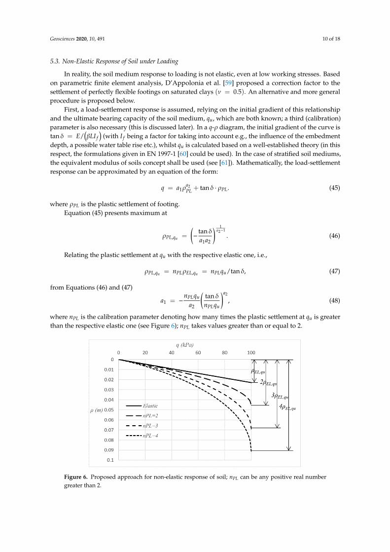
where nPL is the calibration parameter denoting how many times the plastic settlement at qu is greaterthan the respective elastic one (see Figure 6); nPL takes values greater than or equal to 2.Geosciences 2020, 10, x FOR PEER REVIEW 11 of 19

Figure 6. Proposed approach for non-elastic response of soil; PLn can be any positive real number

greater than 2.

The parameter PLn can be estimated based on (a) local experience, i.e., known measured

settlements of neighbor structures, (b) plate bearing test data given that the soil and soil conditions

are relatively homogenous with depth, or (c) 2D plastic finite element analysis by interpolating

between the load-settlement response of the respective axisymmetric and plane strain problem

(circular and strip footing both having radius and width respectively equal to B). The calibration

should refer to similar loading conditions, i.e., drained or undrained.

The plastic settlement, PL , corresponding to q is, finally, obtained from Equation (45). The latter

has two solutions, from which the smaller one is adopted. Depending on the PLn value used,

numerical approximation may be required.

An example q - chart referring to a 1 m × 2 m rigid footing lying on the surface of a semi-

infinite homogenous clay soil with E = 5000 kPa and ν = 0.1 (drained conditions) is given in Figure 6.

In this respect, four q - relationships were drawn, i.e., for perfectly elastic medium and for plastic

medium with PLn =2, 3 and 4. The ultimate bearing capacity value (qu) is equal to 100 kPa. Moreover,

the correction regarding the effect of footing shape on the modulus of soil (recall Equation (26)) was

ignored in this example.

6. Comparison Examples

6.1. Comparison with Existing Methods and Approaches

The proposed method is compared with Mayne and Poulos’ [15] method, as well as with the

“characteristic point” approach [62,63]. Third factors affecting settlement, such as the embedment

depth, soil creep, are ignored, whilst the mass is considered to be semi-infinite and homogenous.

Since Mayne and Poulos’ method deals with footings of any rigidity, both the cases of perfectly

flexible and perfectly rigid footing will be presented. The settlement values obtained from the theory

of elasticity for both the center and the corner of footing, considering that the latter is perfectly flexible

are presented as boundary values (the elastic settlement of the respective rigid footing should be an

intermediate value). The average settlement of perfectly flexible footing is also given. All settlement

expressions used are given in the Appendix B.

Regarding the so-called “characteristic point”, at this point the settlement of a flexible loaded

area is considered to be the same as the uniform settlement of a rigid area, both having the same area

and shape and bearing the same total load. In an ideally elastic soil, the characteristic point at a B L

rectangular footing is located at distance 0.37B and 0.37L from the center [62–65]. What is not widely

known, however, is that the above distances refer to the simple case of ν = 0 [62,63,66].

Figure 6. Proposed approach for non-elastic response of soil; nPL can be any positive real numbergreater than 2.

Geosciences 2020, 10, 491 11 of 18

At the ultimate loading, from Equations (45), (46), and (48):

qu ={a1ρ

a2PL,qu

+ tan δ · ρPL,qu

}= qunPL

a2 − 1a2

, (49)

and solving the latter as for a2:

a2 =nPL

nPL − 1. (50)

The parameter nPL can be estimated based on (a) local experience, i.e., known measured settlementsof neighbor structures, (b) plate bearing test data given that the soil and soil conditions are relativelyhomogenous with depth, or (c) 2D plastic finite element analysis by interpolating between theload-settlement response of the respective axisymmetric and plane strain problem (circular and stripfooting both having radius and width respectively equal to B). The calibration should refer to similarloading conditions, i.e., drained or undrained.

The plastic settlement, ρPL, corresponding to q is, finally, obtained from Equation (45). The latterhas two solutions, from which the smaller one is adopted. Depending on the nPL value used, numericalapproximation may be required.

An example q -ρ chart referring to a 1 m × 2 m rigid footing lying on the surface of a semi-infinitehomogenous clay soil with E = 5000 kPa and ν = 0.1 (drained conditions) is given in Figure 6. In thisrespect, four q -ρ relationships were drawn, i.e., for perfectly elastic medium and for plastic mediumwith nPL = 2, 3 and 4. The ultimate bearing capacity value (qu) is equal to 100 kPa. Moreover, thecorrection regarding the effect of footing shape on the modulus of soil (recall Equation (26)) wasignored in this example.

6. Comparison Examples

6.1. Comparison with Existing Methods and Approaches

The proposed method is compared with Mayne and Poulos’ [15] method, as well as with the“characteristic point” approach [62,63]. Third factors affecting settlement, such as the embedmentdepth, soil creep, are ignored, whilst the mass is considered to be semi-infinite and homogenous.

Since Mayne and Poulos’ method deals with footings of any rigidity, both the cases of perfectlyflexible and perfectly rigid footing will be presented. The settlement values obtained from the theoryof elasticity for both the center and the corner of footing, considering that the latter is perfectly flexibleare presented as boundary values (the elastic settlement of the respective rigid footing should be anintermediate value). The average settlement of perfectly flexible footing is also given. All settlementexpressions used are given in the Appendix B.

Regarding the so-called “characteristic point”, at this point the settlement of a flexible loadedarea is considered to be the same as the uniform settlement of a rigid area, both having the same areaand shape and bearing the same total load. In an ideally elastic soil, the characteristic point at a B× Lrectangular footing is located at distance 0.37B and 0.37L from the center [62–65]. What is not widelyknown, however, is that the above distances refer to the simple case of ν = 0 [62,63,66].

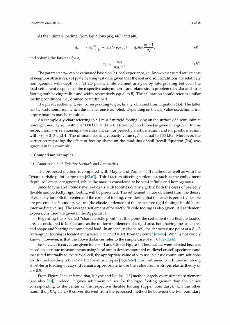
ρE/q vs. L/B curves are given for ν = 0.1 and 0.5; see Figure 7. These values were selected because,based on accurate measurements using local strain devices mounted midlevel on soil specimens andmeasured internally to the triaxial cell, the appropriate value of ν to use in elastic continuum solutionsfor drained loading is 0.1 < ν < 0.2 for all soil types [15,67–69]. For undrained conditions involvingshort-term loading of clays, it remains appropriate to use the value from isotropic elastic theory ofν = 0.5.

From Figure 7 it is inferred that, Mayne and Poulos’ [15] method largely overestimates settlement(see also [70]); indeed, it gives settlement values for the rigid footing greater than the valuescorresponding to the center of the respective flexible footing (upper boundary). On the otherhand, the ρE/q vs. L/B curves derived from the proposed method lie between the two boundary

Geosciences 2020, 10, 491 12 of 18

curves derived from the theory of elasticity, whilst moreover, they are parallel to these boundaries.In addition, the proposed ρE/q − L/B curve for ν = 0.1 compares well with the respective curvecorresponding to the characteristic point. The latter can also be considered indicative of the success ofthe calibration of the proposed method. Furthermore, as shown in Figure 7, the average settlementcurve overestimates settlement for small ν values and underestimates settlement for great ν values.

Geosciences 2020, 10, x FOR PEER REVIEW 12 of 19

E q vs. L B curves are given for ν = 0.1 and 0.5; see Figure 7. These values were selected

because, based on accurate measurements using local strain devices mounted midlevel on soil

specimens and measured internally to the triaxial cell, the appropriate value of ν to use in elastic

continuum solutions for drained loading is 0.1 < ν < 0.2 for all soil types [15,67–69]. For undrained

conditions involving short-term loading of clays, it remains appropriate to use the value from

isotropic elastic theory of ν = 0.5.

From Figure 7 it is inferred that, Mayne and Poulos’ [15] method largely overestimates

settlement (see also [70]); indeed, it gives settlement values for the rigid footing greater than the

values corresponding to the center of the respective flexible footing (upper boundary). On the other

hand, the E q vs. L B curves derived from the proposed method lie between the two boundary

curves derived from the theory of elasticity, whilst moreover, they are parallel to these boundaries.

In addition, the proposed E q − L B curve for ν = 0.1 compares well with the respective curve

corresponding to the characteristic point. The latter can also be considered indicative of the success

of the calibration of the proposed method. Furthermore, as shown in Figure 7, the average settlement

curve overestimates settlement for small ν values and underestimates settlement for great ν values.

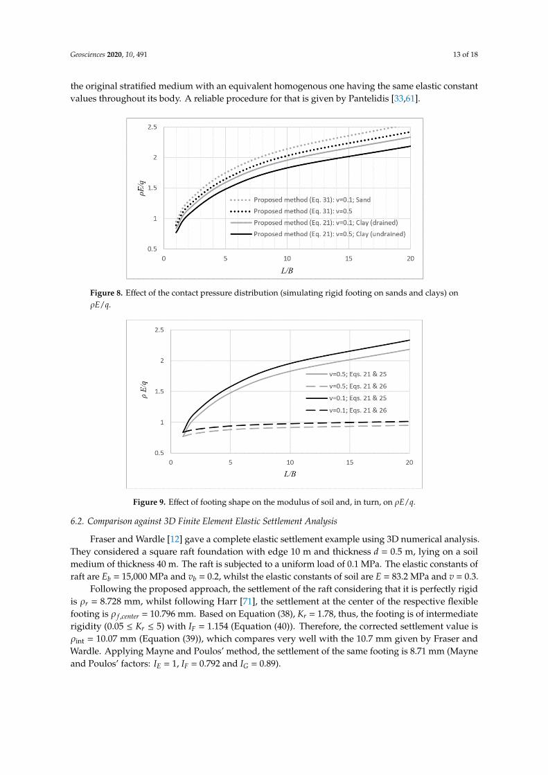
In addition, from Figure 8 it is inferred that for the same ν value, the E q term for the rigid

footing on sand is greater than the respective one for the same footing on clay. The goal of Figure 8

is to compare the effect of the different contact pressure distributions, assuming the same E value,

which is also constant with depth. In reality, E may vary with depth; this is usually observed in sands,

where E increases with depth (Gibson profile [32]), even immediately after deposition [29]. It is also

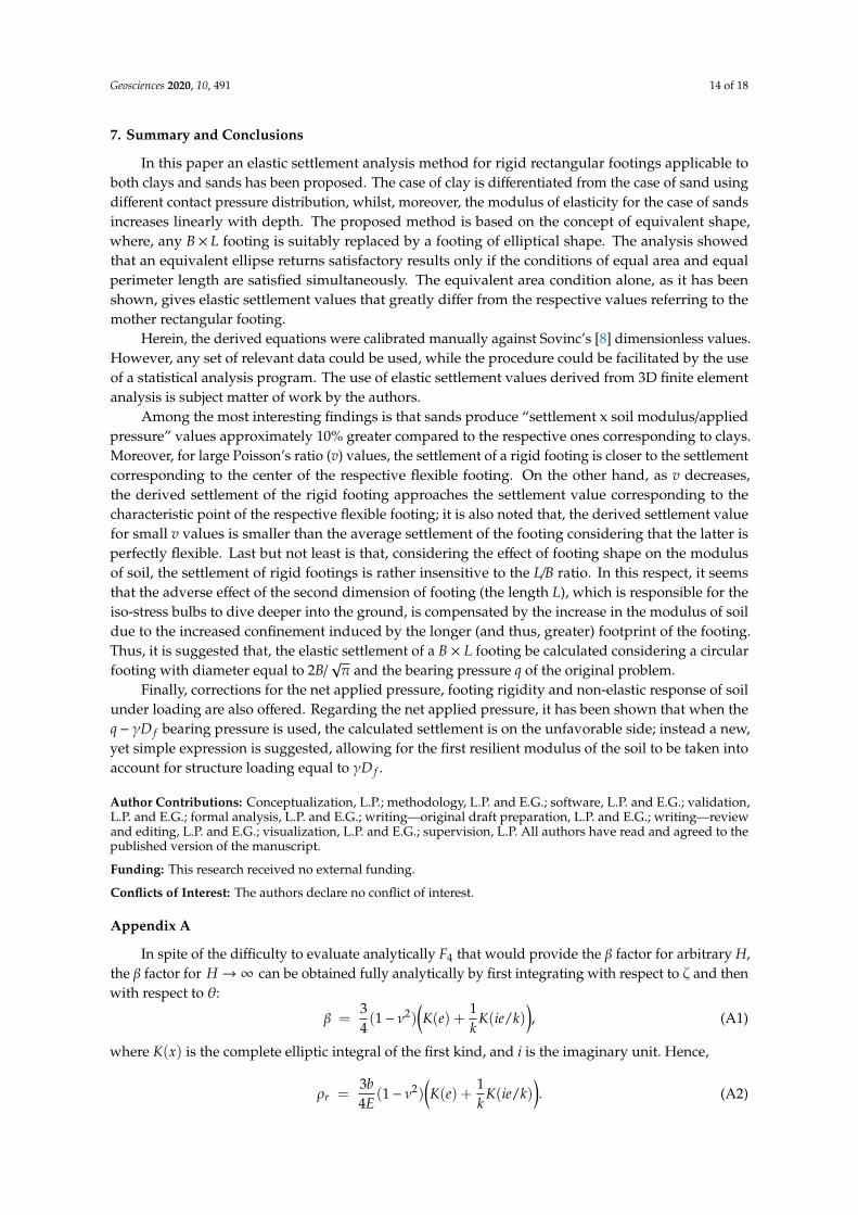
very interesting that, as shown in Figure 9, when the effect of footing shape on the modulus of

elasticity of soil is considered in the analysis, the L B ratio of footing has, practically, minor effect

on the derived settlement. In this respect, revisiting existing experimental and theoretical studies,

Pantelidis [29,30] draw the conclusion that the elastic settlement appears to be independent of the

aspect ratio of footing; it seems that the adverse effect of the second dimension of footing, which is

responsible for the iso-stress bulbs to dive deeper into the ground, is compensated by the increase in

E due to the increased confinement induced by the longer (and thus, greater) footprint of the footing.

In this respect, he suggested that, the elastic settlement of a B × L footing be calculated considering a

circular footing with diameter equal to B (or better, 2B/ ) and the bearing pressure q of the original

problem. A problem, however, arises when soil medium is stratified. This can be solved by replacing

the original stratified medium with an equivalent homogenous one having the same elastic constant

values throughout its body. A reliable procedure for that is given by Pantelidis [33,61].

Geosciences 2020, 10, x FOR PEER REVIEW 13 of 19

Figure 7. Comparison example: (a) v = 0.1 and (b) v = 0.5.

Figure 8. Effect of the contact pressure distribution (simulating rigid footing on sands and clays) on

E q .

Figure 9. Effect of footing shape on the modulus of soil and, in turn, on E q .

6.2. Comparison against 3D Finite Element Elastic Settlement Analysis

Fraser and Wardle [12] gave a complete elastic settlement example using 3D numerical analysis.

They considered a square raft foundation with edge 10 m and thickness d = 0.5 m, lying on a soil

Figure 7. Comparison example: (a) v = 0.1 and (b) v = 0.5.

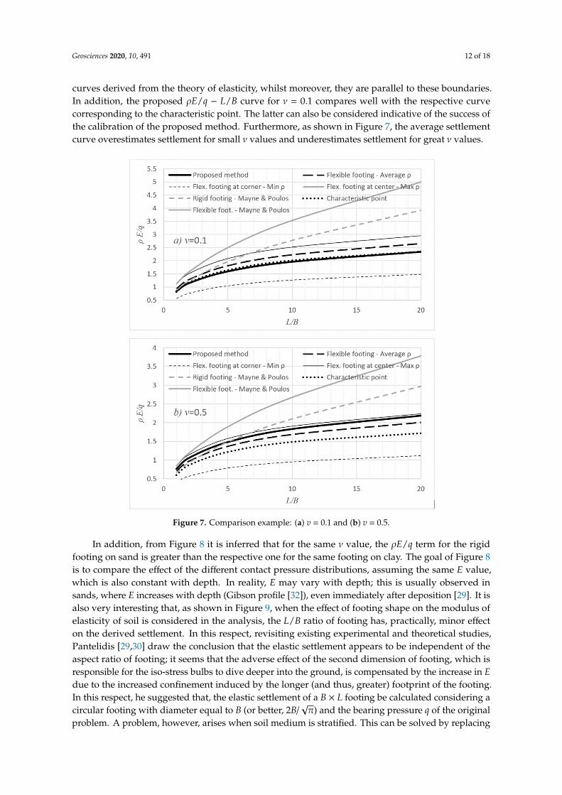
In addition, from Figure 8 it is inferred that for the same ν value, the ρE/q term for the rigidfooting on sand is greater than the respective one for the same footing on clay. The goal of Figure 8is to compare the effect of the different contact pressure distributions, assuming the same E value,which is also constant with depth. In reality, E may vary with depth; this is usually observed insands, where E increases with depth (Gibson profile [32]), even immediately after deposition [29]. It isalso very interesting that, as shown in Figure 9, when the effect of footing shape on the modulus ofelasticity of soil is considered in the analysis, the L/B ratio of footing has, practically, minor effecton the derived settlement. In this respect, revisiting existing experimental and theoretical studies,Pantelidis [29,30] draw the conclusion that the elastic settlement appears to be independent of theaspect ratio of footing; it seems that the adverse effect of the second dimension of footing, which isresponsible for the iso-stress bulbs to dive deeper into the ground, is compensated by the increase in Edue to the increased confinement induced by the longer (and thus, greater) footprint of the footing.In this respect, he suggested that, the elastic settlement of a B × L footing be calculated considering acircular footing with diameter equal to B (or better, 2B/

√π) and the bearing pressure q of the original

problem. A problem, however, arises when soil medium is stratified. This can be solved by replacing

Geosciences 2020, 10, 491 13 of 18

the original stratified medium with an equivalent homogenous one having the same elastic constantvalues throughout its body. A reliable procedure for that is given by Pantelidis [33,61].

Geosciences 2020, 10, x FOR PEER REVIEW 13 of 19

Figure 7. Comparison example: (a) v = 0.1 and (b) v = 0.5.

Figure 8. Effect of the contact pressure distribution (simulating rigid footing on sands and clays) on

E q .

Figure 9. Effect of footing shape on the modulus of soil and, in turn, on E q .

6.2. Comparison against 3D Finite Element Elastic Settlement Analysis

Fraser and Wardle [12] gave a complete elastic settlement example using 3D numerical analysis.

They considered a square raft foundation with edge 10 m and thickness d = 0.5 m, lying on a soil

Figure 8. Effect of the contact pressure distribution (simulating rigid footing on sands and clays) onρE/q.

Geosciences 2020, 10, x FOR PEER REVIEW 13 of 19

Figure 7. Comparison example: (a) v = 0.1 and (b) v = 0.5.

Figure 8. Effect of the contact pressure distribution (simulating rigid footing on sands and clays) on

E q .

Figure 9. Effect of footing shape on the modulus of soil and, in turn, on E q .

6.2. Comparison against 3D Finite Element Elastic Settlement Analysis

Fraser and Wardle [12] gave a complete elastic settlement example using 3D numerical analysis.

They considered a square raft foundation with edge 10 m and thickness d = 0.5 m, lying on a soil

Figure 9. Effect of footing shape on the modulus of soil and, in turn, on ρE/q.

6.2. Comparison against 3D Finite Element Elastic Settlement Analysis

Fraser and Wardle [12] gave a complete elastic settlement example using 3D numerical analysis.They considered a square raft foundation with edge 10 m and thickness d = 0.5 m, lying on a soilmedium of thickness 40 m. The raft is subjected to a uniform load of 0.1 MPa. The elastic constants ofraft are Eb = 15,000 MPa and vb = 0.2, whilst the elastic constants of soil are E = 83.2 MPa and v = 0.3.

Following the proposed approach, the settlement of the raft considering that it is perfectly rigidis ρr = 8.728 mm, whilst following Harr [71], the settlement at the center of the respective flexiblefooting is ρ f ,center = 10.796 mm. Based on Equation (38), Kr = 1.78, thus, the footing is of intermediaterigidity (0.05 ≤ Kr ≤ 5) with IF = 1.154 (Equation (40)). Therefore, the corrected settlement value isρint = 10.07 mm (Equation (39)), which compares very well with the 10.7 mm given by Fraser andWardle. Applying Mayne and Poulos’ method, the settlement of the same footing is 8.71 mm (Mayneand Poulos’ factors: IE = 1, IF = 0.792 and IG = 0.89).

Geosciences 2020, 10, 491 14 of 18

7. Summary and Conclusions

In this paper an elastic settlement analysis method for rigid rectangular footings applicable toboth clays and sands has been proposed. The case of clay is differentiated from the case of sand usingdifferent contact pressure distribution, whilst, moreover, the modulus of elasticity for the case of sandsincreases linearly with depth. The proposed method is based on the concept of equivalent shape,where, any B × L footing is suitably replaced by a footing of elliptical shape. The analysis showedthat an equivalent ellipse returns satisfactory results only if the conditions of equal area and equalperimeter length are satisfied simultaneously. The equivalent area condition alone, as it has beenshown, gives elastic settlement values that greatly differ from the respective values referring to themother rectangular footing.

Herein, the derived equations were calibrated manually against Sovinc’s [8] dimensionless values.However, any set of relevant data could be used, while the procedure could be facilitated by the useof a statistical analysis program. The use of elastic settlement values derived from 3D finite elementanalysis is subject matter of work by the authors.

Among the most interesting findings is that sands produce “settlement x soil modulus/appliedpressure” values approximately 10% greater compared to the respective ones corresponding to clays.Moreover, for large Poisson’s ratio (v) values, the settlement of a rigid footing is closer to the settlementcorresponding to the center of the respective flexible footing. On the other hand, as v decreases,the derived settlement of the rigid footing approaches the settlement value corresponding to thecharacteristic point of the respective flexible footing; it is also noted that, the derived settlement valuefor small v values is smaller than the average settlement of the footing considering that the latter isperfectly flexible. Last but not least is that, considering the effect of footing shape on the modulusof soil, the settlement of rigid footings is rather insensitive to the L/B ratio. In this respect, it seemsthat the adverse effect of the second dimension of footing (the length L), which is responsible for theiso-stress bulbs to dive deeper into the ground, is compensated by the increase in the modulus of soildue to the increased confinement induced by the longer (and thus, greater) footprint of the footing.Thus, it is suggested that, the elastic settlement of a B × L footing be calculated considering a circularfooting with diameter equal to 2B/

√π and the bearing pressure q of the original problem.

Finally, corrections for the net applied pressure, footing rigidity and non-elastic response of soilunder loading are also offered. Regarding the net applied pressure, it has been shown that when theq− γD f bearing pressure is used, the calculated settlement is on the unfavorable side; instead a new,yet simple expression is suggested, allowing for the first resilient modulus of the soil to be taken intoaccount for structure loading equal to γD f .

Author Contributions: Conceptualization, L.P.; methodology, L.P. and E.G.; software, L.P. and E.G.; validation,L.P. and E.G.; formal analysis, L.P. and E.G.; writing—original draft preparation, L.P. and E.G.; writing—reviewand editing, L.P. and E.G.; visualization, L.P. and E.G.; supervision, L.P. All authors have read and agreed to thepublished version of the manuscript.

Funding: This research received no external funding.

Conflicts of Interest: The authors declare no conflict of interest.

Appendix A

In spite of the difficulty to evaluate analytically F4 that would provide the β factor for arbitrary H,the β factor for H→∞ can be obtained fully analytically by first integrating with respect to ζ and thenwith respect to θ:

β =34(1− ν2)

(K(e) +

1k

K(ie/k)), (A1)

where K(x) is the complete elliptic integral of the first kind, and i is the imaginary unit. Hence,

ρr =3b4E

(1− ν2)(K(e) +

1k

K(ie/k)). (A2)

Geosciences 2020, 10, 491 15 of 18

For the case of circular footing (k = 1) over sand, Equation (33) simplifies to

Iz = 3(ν+ 1)(

12(1 + ζ2)

− ν(1− ζ cot−1 ζ

)), (A3)

and by integrating the latter from z = 0 to H, we get the factor β

β =34(ν+ 1)

(ν(ν

Hb− 2

)(Hb

)+ 2

(1− ν− ν

(Hb

)2)tan−1

(Hb

)). (A4)

For H→∞ Equation (A4) gives

β =3π4(1− ν2), (A5)

and, thus, the settlement expression becomes

ρr =3πqa4E

(1− ν2

)= 1.5

(πqa2E

(1− ν2

)), (A6)

meaning that the term ρrE/q for a circular rigid footing on sands is by 50% greater than the respectiveone for clays.

Appendix B

Settlement under the corner and center of a B× L (flexible) rectangular footing [71]

ρ(z) =accqB′

2Es

(1− ν2

)(Acc −

1− 2ν1− ν

Bcc

), (A7)

Acc =1π

ln

√1 + m2 + n2 + m√

1 + m2 + n2 −m+ m ln

√1 + m2 + n2 + 1√

1 + m2 + n2 − 1

, (A8)

Bcc =nπ

tan−1 m

n√

1 + m2 + n2, (A9)

with acc = 1, B′ = B, m = L/B and n = z/B for the corner of the footing, whilst acc = 4, B′ = B/2,m = L/B and n = 2z/B for the center; z = 0 (and thus, n = 0) for the settlement on the surface of ahomogenous, semi-infinite mass. For the settlement of footing underlain by a layer of finite thicknessH, the principle of superposition stands, i.e., ρ = ρ(0) − ρ(H).

Average settlement of a B× L (flexible) rectangular footing on semi-infinite homogenous mass [72]

ρ(z) =q√

BLEs

(1− ν2

)Aav, (A10)

Aav =1

π√

m

ln

√1 + m2 + m√

1 + m2 −m+ m ln

√1 + m2 + 1√

1 + m2 − 1−

23

(1 + m2

) 32−

(1 + m3

)m

, (A11)

with m as defined above.Mayne and Poulos [15] expressed the settlement as follows:

ρ(z) =qEs

√4BLπ

(1− ν2

)IGIFIE, (A12)

where IF = π/4 and 1 for perfectly rigid and perfectly flexible footing respectively, IE = 1 forfoundation on the surface and IG = 1 for homogenous, semi-infinite mass. For more about theI-factors, please see the original publication [15].

Geosciences 2020, 10, 491 16 of 18

References

1. Noble, B. The numerical solution of the singular integral equation for the charge distribution on a flatrectangular plate. In Proceedings of the PICC Symposium on Differential and Integral Equations, Rome,Italy, 20–24 September 1960; Birkhäuser: Basel, Switzerland; Stuttgart, Germany, 1960; pp. 530–543.

2. Borodachev, N.M.; Galin, L.A. Contact problem for a stamp with narrow rectangular base: PMM vol. 38,n$ 1, 1974, pp. 125–130. J. Appl. Math. Mech. 1974, 38, 108–113. [CrossRef]

3. Gorbunov-Possadov, M.; Serebrjanyi, R. Design of Structures on Elastic Foundations. In Proceedings of theFifth International Conference on Soil Mechanics and Foundation Engineering, 17–22 July, 1961; Dunod: Paris,France, 1961; pp. 643–648.

4. Borodachev, N.M. Contact problem for a stamp with a rectangular base: PMM vol. 40, n$ 3, 1976, pp. 554–560.J. Appl. Math. Mech. 1976, 40, 505–512. [CrossRef]

5. Mullan, S.J.; Sinclair, G.B.; Brothers, P.W. Stresses for an elastic half-space uniformly indented by a rigidrectangular footing. Int. J. Numer. Anal. Methods Geomech. 1980, 4, 277–284. [CrossRef]

6. Brothers, P.W.; Sinclair, G.B.; Segedin, C.M. Uniform indentation of the elastic half-space by a rigid rectangularpunch. Int. J. Solids Struct. 1977, 13, 1059–1072. [CrossRef]

7. Panek, C.; Kalker, J.J. A solution for the narrow rectangular punch. J. Elast. 1977, 7, 213–218. [CrossRef]8. Sovinc, I. Displacements and inclinations of rigid footings resting on a limited elastic layer on uniform

thickness. In Proceedings of the 7th International Conference on Soil Mechanics and Foundation Engineering;Sociedad Mexicana de Mecanica: Mexico City, Mexico, 1961; pp. 385–389.

9. Dempsey, J.P.; Li, H. A rigid rectangular footing on an elastic layer. Géotechnique 1989, 39, 147–152. [CrossRef]10. Butterfield, R.; Banerjee, P.K. A rigid disc embedded in an elastic half space. Geotech. Eng. 1971, 2, 35–52.11. Fabrikant, V.I. Flat punch of arbitrary shape on an elastic half-space. Int. J. Eng. Sci. 1986, 24, 1731–1740.

[CrossRef]12. Fraser, R.A.; Wardle, L.J. Numerical analysis of rectangular rafts on layered foundations. Géotechnique 1976,

26, 613–630. [CrossRef]13. Schmertmann, J.H. Static cone to compute static settlement over sand. J. Soil Mech. Found. Div. 1970, 96,

1011–1043.14. Schmertmann, J.H.; Hartman, J.P.; Brown, P.R. Improved strain influence factor diagrams. J. Geotech.

Geoenviron. Eng. 1978, 104, 1131–1135.15. Mayne, P.W.; Poulos, H.G. Approximate displacement influence factors for elastic shallow foundations.

J. Geotech. Geoenviron. Eng. 1999, 125, 453–460. [CrossRef]16. Foye, K.C.; Basu, P.; Prezzi, M. Immediate Settlement of Shallow Foundations Bearing on Clay. Int. J. Geomech.

2008, 8, 300–310. [CrossRef]17. Lee, J.; Salgado, R. Estimation of footing settlement in sand. Int. J. Geomech. 2002, 2, 1–28. [CrossRef]18. Schiffman, R.L.; Aggarwala, B.D. Stresses and displacements produced in a semi-infinite elastic solid by a

rigid elliptical footing. In Proceedings of the 5th International Conference on Soil Mechanics and FoundationEngineering, Paris, France, 17–22 July 1961; Dunod: Paris, France, 1961; Volume 1, pp. 795–801.

19. Boussinesq, J. Application des Potentiels à L’étude de L’équilibre et du Mouvement des Solides Élastiques:Principalement au Calcul des Déformations et des Pressions que Produisent, dans ces Solides, des Efforts QuelconquesExercés sur une Petite Partie de Leur Surface; Gauthier-Villars: Paris, France, 1885; Volume 4.

20. Das, B.M. Fundamentals of Geotechnical Engineering, 3rd ed.; Thomson-Engineering: Mobile, AL, USA, 2007;ISBN 10:0-495-29572-8.

21. Hudson, J.A.; Harrison, J.P. Engineering Rock Mechanics: An Introduction to the Principles; Elsevier: Amsterdam,The Netherlands, 2000; ISBN 0080530966.

22. Sadd, M.H. Elasticity: Theory, Applications, and Numerics; Academic Press: Cambridge, MA, USA, 2009;ISBN 0080922414.

23. Pantelidis, L. Strain Influence Factor Charts for Settlement Evaluation of Spread Foundations based on theStress–Strain Method. Appl. Sci. 2020, 10, 3822. [CrossRef]

24. Kézdi, Á.; Rétháti, L. Soil Mechanics of Earthworks, Foundations and Highway Engineering, Handbook of SoilMechanics; Elsevier: New York, NY, USA, 1988; Volume 3, ISBN 0-444-98929-3.

25. Abramowitz, M.; Stegun, I.A. Handbook of Mathematical Functions: With Formulas, Graphs, and MathematicalTables; Courier Corporation: North Chelmsford, MA, USA, 1965; Volume 55, ISBN 0486612724.

Geosciences 2020, 10, 491 17 of 18

26. Das, B.M. Shallow Foundations: Bearing Capacity and Settlement, 3rd ed.; CRC Press: Boca Raton, FL, USA,2017; ISBN 9781315163871.

27. Poulos, H.G.; Davis, E.H. Elastic Solutions for Soil and Rock Mechanics; John Wiley: New York, NY, USA, 1991;ISBN 0471695653.

28. Terzaghi, K.; Peck, R.B.; Mesri, G. Soil Mechanics in Engineering Practice; John Wiley: New York, NY, USA,1996; ISBN 0471086584.

29. Pantelidis, L. Elastic Settlement Analysis for Various Footing Cases Based on Strain Influence Areas.Geotech. Geol. Eng. 2020, 38, 4201–4225. [CrossRef]

30. Pantelidis, L. The effect of footing shape on the elastic modulus of soil. In Proceedings of the 2nd Conferenceof the Arabian Journal of Geosciences (CAJG), Sousse, Tunisia, 25–28 November 2019; Springer Nature:Sousse, Tunisia, 2019.

31. Barnes, G. Soil Mechanics: Principles and Practice; Palgrave Macmillan: London, UK, 2016; ISBN 1137512210.32. Gibson, R.E. Some Results Concerning Displacements and Stresses in a Non-Homogeneous Elastic Half-space.

Géotechnique 1967, 17, 58–67. [CrossRef]33. Pantelidis, L. On the modulus of subgrade reaction for shallow foundations on homogenous or stratified

mediums. In Proceedings of the 3rd International Structural Engineering and Construction Conference(EURO-MED-SEC-03), Limassol, Cyprus, 3–8 August 2020; Vacanas, Y., Danezis, C., Yazdani, S., Singh, A.,Eds.; ISEC Press: Limassol, Cyprus, 2020.

34. Fox, L. The mean elastic settlement of a uniformly loaded area at a depth below the ground surface.In Proceedings of the Second International Conference on Soil Mechanics and Foundation Engineering,Rotterdam, The Netherlands, 21–30 June 1948; Volume 1, p. 129.

35. Janbu, N.; Bjerrum, L.; Kjaernsli, B. Veiledning ved lo/sniffing av fundamenterings oppgaver. In Norwegianwith English Summary; Soil Mechanics Applied to Some Engineering Problems; Norwegian Geotechnical Institute,Publication: Oslo, Norway, 1956.

36. Burland, J.B. Discussion of session A. In Proc. of the Conf. on In Situ Investigations in Soils and Rocks; BritishGeotechnical Society: London, UK, 1970; pp. 61–62.

37. Christian, J.; Carrier, D. Janbu, Bjerrum and Kjaernsli’s chart reinterpreted. Can. Geotech. J. 1978, 15, 123–128.[CrossRef]

38. Díaz, E.; Tomás, R. Revisiting the effect of foundation embedment on elastic settlement: A new approach.Comput. Geotech. 2014, 62, 283–292. [CrossRef]

39. Teng, W.C. Foundation Design; Prendice-Hall Inc.: New York, NY, USA, 1962.40. Alpan, I. Estimating the settlements of foundations on sands. Civ. Eng Public Work. Rev. UK 1964, 59,

1415–1418.41. Bazaraa, A.R. Use of the Standard Penetration Test for Estimating Settlements of Shallow Foundations on Sand;

University of Illinois: Champaign, IL, USA, 1967.42. Bowles, L.E. Foundation Analysis and Design; McGraw-Hill: New York, NY, USA, 1996; ISBN 0079122477.43. Peck, R.B.; Hanson, W.E.; Thornburn, T.H. Foundation Engineering; Wiley: New York, NY, USA, 1974;

Volume 10.44. Terzaghi, K.; Peck, R.B. Soil Mechanics in Engineering Practice; John and Wiley and Sons: Hoboken, NJ, USA,

1967; ISBN 0471852732.45. Agarwal, K.B.; Rana, M.K. Effect of ground water on settlement of footings in sand. In Proceedings

of the 9th European Conference on Soil Mechanics and Foundation Engineering, Dublin, Ireland,31 August–3 September 1987; Balkema: Rotterdam, The Netherlands, 1987; pp. 751–754.

46. NAVFAC. Soil Mechanics Design Manual (NAVFAC DM 7.1); Naval Facilities Engineering Command:Alexandria, VA, USA, 1982.

47. Shahriar, M.A.N.; Sivakugan, N.; Das, B.M. Settlement correction for future water table rise in granular soils:A numerical modelling approach. Int. J. Geotech. Eng. 2013, 7, 214–217. [CrossRef]

48. Shahriar, M.A.; Sivakugan, N.; Das, B.M.; Urquhart, A.; Tapiolas, M. Water Table Correction Factors forSettlements of Shallow Foundations in Granular Soils. Int. J. Geomech. 2015, 15, 06014015. [CrossRef]

49. Ulrich, E.J.; Shukla, S.N.; Baker, C.N., Jr.; Ball, S.C.; Bowles, J.E.; Colaco, J.P.; Davisson, T.; Focht, J.A., Jr.;Gaynor, M.; Gnaedinger, J.P.; et al. Suggested analysis and design procedures for combined footings andmats. J. Am. Concr. Inst. 1988, 86, 304–324.

Geosciences 2020, 10, 491 18 of 18

50. DIN 4018 Berechnung der Sohldruckverteilung unter Flächengründungen Einschl; Deutsche Normen: Berlin,Germany, 1974.

51. IS 2950-1 Code of Practice for Design and Construction of Raft Foundations, Part 1: Design IS 1904:1986 Code forPractice, Design and Construction of Foundations in Soil; Bureau of Indian Standards: New Delhi, India, 1981.

52. Varghese, P.C. Foundation Engineering; PHI Learning Pvt. Ltd.: Delhi, India, 2005; ISBN 8120326520.53. Milovic, D. Stresses and Displacements for Shallow Foundations; Elsevier: Amsterdam, The Netherlands, 1992;

ISBN 0-444-88349-5.54. Brown, P.T. Numerical analyses of uniformly loaded circular rafts on deep elastic foundations. Geotechnique

1969, 19, 399–404. [CrossRef]55. Duncan, J.M.; Buchignani, A.L. An Engineering Manual for Settlement Studies; Department of Civil Engineering,

University of California: Berkley, CA, USA, 1976.56. US Army Corps of Engineers. Engineering and Design-Settlement Analysis, EM 1110-1904; U.S. Army Corps of

Engineers: Washington, DC, USA, 1990.57. Mayne, P.W.; Kulhawy, F.H. K0-OCR relationships in soil. J. Geotech. Eng. 1982, 108, 851–872.58. Mesri, G.; Ullrich, C.R.; Choi, Y.K. The rate of swelling of overconsolidated clays subjected to unloading.

Géotechnique 1978, 28, 281–307. [CrossRef]59. D’Appolonia, D.J.; Poulos, H.G.; Ladd, C.C. Initial settlement of of structures on clay. J. Soil Mech. Found.

Div. ASCE 1971, 97, 1359–1377.60. EN 1997-1. Eurocode 7 Geotechnical Design—Part 1: General Rules; European Committee for Standardization

(CEN): Brussels, Belgium, 2004.61. Pantelidis, L. The equivalent modulus of elasticity of layered soil mediums for designing shallow foundations

with the Winkler spring hypothesis: A critical review. Eng. Struct. 2019, 201, 109452. [CrossRef]62. Kany, M. Berechnung von Flächengründungen, 2nd ed.; Ernst u. Sohn: Berlin, Germany, 1974.63. Grasshoff, H. Setzungsberechnungen starrer Fundamente mit Hilfe des kennzeichnenden Punktes.

Bauingenieur 1955, 30, 53–54.64. Kaniraj, S.R. Design Aids in Soil Mechanics and Foundation Engineering; Tata McGraw-Hill: New York, NY,

USA, 1988; ISBN 0074517147.65. Fellenius, B.H. Basics of Foundation Design; BC BiTech Publishers Limited: Richmond, BC, Canada, 2006.66. Kempfert, H.-G.; Gebreselassie, B. Excavations and Foundations in Soft Soils; Springer Science & Business

Media: Berlin, Germany, 2006; ISBN 3540328955.67. Tatsuoka, F.; Teachavorasinskun, S.; Dong, J.; Kohata, Y.; Sato, T. Importance of Measuring Local Strains

in Cyclic Triaxial Tests on Granular Materials. In Dynamic Geotechnical Testing II; ASTM International:West Conshohocken, PA, USA, 1994; pp. 288–302.

68. Jamiolkowski, M.; Lancellotta, R.; LoPresti, D.C.F. Remarks on the stiffness at small strains of six Italianclays. In Proceedings of the Int. Symp. on Pre-Failure Deformation of Geomaterials, Sapporo, Japan,12–14 September 1994; Balkema: Rotterdam, The Netherlands, 1995; pp. 817–836.

69. Pincus, H.; Lo Presti, D.; Pallara, O.; Puci, I. A Modified Commercial Triaxial Testing System for Small StrainMeasurements: Preliminary Results on Pisa Clay. Geotech. Test. J. 1995, 18, 15. [CrossRef]

70. Cho, H.; Kim, N.; Park, H.; Kim, D. Settlement Prediction of Footings Using VS. Appl. Sci. 2017, 7, 1105.[CrossRef]

71. Harr, M.E. Foundations of Theoretical Soil Mechanics; McGraw-Hill Inc.: New York, NY, USA, 1966;ISBN 10:0070267413.

72. Schleicher, F. Schleicher Zur Theorie der Baugrundes. Bauingenieur 1926, 48, 931–935.

Publisher’s Note: MDPI stays neutral with regard to jurisdictional claims in published maps and institutionalaffiliations.

© 2020 by the authors. Licensee MDPI, Basel, Switzerland. This article is an open accessarticle distributed under the terms and conditions of the Creative Commons Attribution(CC BY) license (http://creativecommons.org/licenses/by/4.0/).