www.elsevier.com/locate/compgeo

Computers and Geotechnics 32 (2005) 445–457

Bearing capacity of circular footings under surcharge usingstate-dependent finite element analysis

Junhwan Lee a,*, Rodrigo Salgado b, Sooil Kim a

a School of Civil and Environmental Engineering, Yonsei University, Seoul, South Koreab School of Civil Engineering, Purdue University, West Lafayette, IN 47907-1284, United States

Received 19 April 2004; received in revised form 30 May 2005; accepted 20 July 2005

Abstract

Footings are often used to support structures at sites where the soils near the surface are sufficiently strong to serve as a bearing layer.In this study, estimation of the bearing capacity of footings resting on a soil mass acted upon by a surcharge is investigated and related tothe cone resistance qc. Non-linear finite element analyses based on a state-dependent stress–strain model were performed to obtain theload–settlement responses of axially loaded circular footings. Various values of relative density, lateral earth pressure ratio, depth ofembedment and footing diameter were considered in the analyses. Based on the finite element results, load–settlement curves wereobtained and used to determine the unit limit bearing capacity of the footings in terms of the cone resistance qc. Values of the unit bearingcapacity for different values of surcharge were in a narrow range, while considerable variation in unit bearing capacity was observed withrelative density DR. It was observed that the unit limit bearing capacity for a given surcharge, normalized with respect to qc, decreases asDR increases, with rates of change depending on the lateral earth pressure ratio K0. The effect of K0 was greater for lower DR values.� 2005 Elsevier Ltd. All rights reserved.

Keywords: Footings; Surcharge; Bearing capacity; CPT; Sands; Non-linear stress–strain model

1. Introduction

Footings are often used to support structures at siteswhere the soils near the surface are sufficiently strong toserve as a bearing layer. The bearing capacity of footingshas been studied both experimentally and theoreticallyfor decades. A common approach to evaluate the bearingcapacity of a footing is the use of the bearing capacityequation, which requires knowledge of the shear strengthparameters of the foundation soil. Since the full descriptionof the bearing capacity equation was first proposed by Ter-zaghi [1], most efforts have focused on developing morerealistic expressions for the bearing capacity factors [2–7].

The use of the bearing capacity equation is subjected toseveral uncertainties. Significant uncertainties include those

0266-352X/$ - see front matter � 2005 Elsevier Ltd. All rights reserved.

doi:10.1016/j.compgeo.2005.07.005

* Correspponding author.E-mail addresses: junlee@yonsei.ac.kr (J.Lee), rodrigo@ecn.purdue.edu

(R. Salgado).

associated with assumptions made for the derivation of thebearing capacity equation, such as the assumption thatsuperposition applies, and for the determination of bearingcapacity factors. The factors Nc and Nq appearing in thebearing capacity equation can be determined rigorouslyfor a strip footing on a deposit of weightless soil with con-stant friction angle. The factor Nc can be determined rigor-ously for a strip footing on a cohesionless deposit in theabsence of a surcharge. However, these factors do notapply to a strip footing on a soil that has non-zero weight,q, c and /. Additionally, the expressions for the shape,depth, load inclination and base and ground inclinationfactors that are necessary to tackle more realistic problemsare at the present time approximate and thus introduceadditional uncertainties into the calculation of bearingcapacity.

Other important uncertainties are related to the valueof the soil friction angle / necessary for the evaluationof the various terms in the bearing capacity equation. It

600

800

1000

Michalowski (smooth) Michalowski (rough)

Bolton and Lau (smooth) Bolton and Lau (rough)

446 J. Lee et al. / Computers and Geotechnics 32 (2005) 445–457

is known that the friction angle / is a function of soilstate, varying notably with the stress state and the soildensity [8–10]. This indicates that the mobilized value ofthe friction angle will vary along the slip surface. Thisrequires a process by which a representative value of /can be selected for given footing and soil conditions.When a surcharge exists, further variation of the frictionangle is expected as the magnitude of the confining stressincreases. The experimental procedures available for theestimation of / add to the uncertainties. As undisturbedsoil sampling is rarely possible in sands, estimation of /in general relies on in situ test results, which introducetheir own uncertainties.

In this paper, we study the bearing capacity of circularfootings in the presence of a surcharge. The study aimsat obtaining accurate relationships for the bearing capacityfactors in terms of the state-dependent shear strength of thesoil, as well as at correlating the bearing capacity of thefooting with cone resistance qc. The load response of axi-ally loaded, circular footings placed on a sand mass sub-jected to a surcharge taking a range of values is obtainedusing non-linear finite element analysis with a state-depen-dent stress–strain model. The load–settlement response ofeach footing analyzed is then interpreted to obtain the nor-malized limit unit bearing capacity. A cone resistance anal-ysis produces the corresponding cone resistance qc, which isused to normalize the bearing capacity. The effects of therelative density DR and lateral earth pressure ratio K0 onthe normalized footing bearing capacity are discussed aswell.

2. Uncertainties in use of bearing capacity equation

2.1. Bearing capacity factors

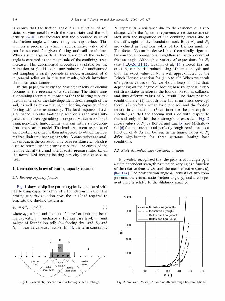
Fig. 1 shows a slip-line pattern typically associated withthe bearing capacity failure of a foundation in sand. Thebearing capacity equation gives the unit load required togenerate the slip-line pattern as:

qbL ¼ qNq þ 12cBN c; ð1Þ

where qbL = limit unit load at ‘‘failure’’ or limit unit bear-ing capacity; q = surcharge at footing base level; c = unitweight of foundation soil; B = footing size; and Nq andNc = bearing capacity factors. In (1), the term containing

B

qbLq

α α

q

passive passive active zone zone zone radial radial shear zone shear zone

Fig. 1. General slip mechanism of a footing under surcharge.

Nq represents a resistance due to the existence of a sur-charge, while the Nc term represents a resistance associ-ated with the magnitude of the confining stress due tothe self-weight of the foundation soil. Both Nq and Nc

are defined as functions solely of the friction angle /.The factor Nq can be derived in a theoretically rigorousfashion for a homogenous, weightless soil with a constantfriction angle. Although a variety of expressions for Nc

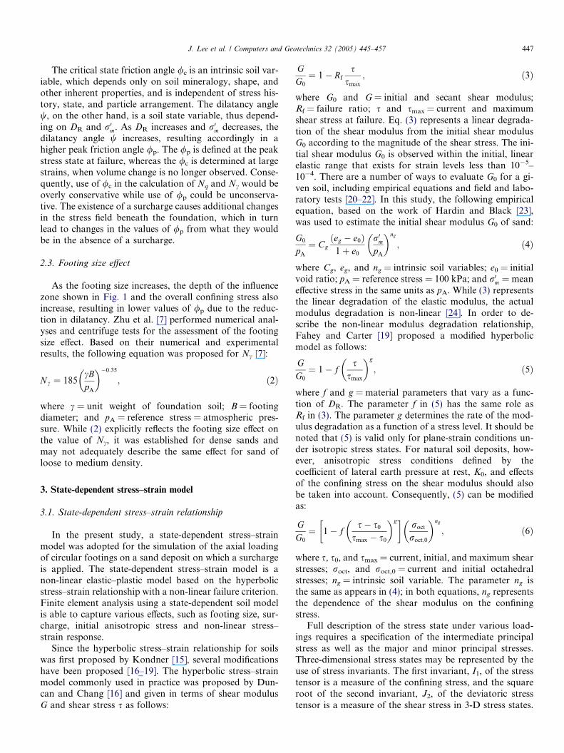
exist [1,3,4,6,7,11,12], Lyamin et al. [13] showed that anexact Nc can be determined using 3D limit analysis andthat this exact value of Nc is well approximated by theBrinch Hansen equation for / up to 40�. When we speakof rigorous values of Nc, we should keep in mind that,depending on the degree of footing base roughness, differ-ent stress states develop in the foundation soil at collapse,and thus different values of Nc result. The three possibleconditions are: (1) smooth base (no shear stress developsthere), (2) perfectly rough base (the soil and the footingremain in contact) and (3) an interface shear strength isspecified, so that the footing will slide with respect tothe soil only if this shear strength is exceeded. Fig. 2shows values of Nc by Bolton and Lau [5] and Michalow-ski [6] for the smooth and perfectly rough conditions as afunction of /. As can be seen in the figure, values of Nc

differ significantly for these extreme footing baseconditions.

2.2. State-dependent shear strength of sands

It is widely recognized that the peak friction angle /p isa state-dependent strength parameter, varying as a functionof the relative density DR and the mean effective stress r0

m

[8–10,14]. The peak friction angle /p consists of two com-ponents, the critical state friction angle /c and a compo-nent directly related to the dilatancy angle w.

0

200

400

0 10 20 30 40 50 60φ ' (o)

Nγ

Fig. 2. Values of Nc with / 0 for smooth and rough base conditions.

J. Lee et al. / Computers and Geotechnics 32 (2005) 445–457 447

The critical state friction angle /c is an intrinsic soil var-iable, which depends only on soil mineralogy, shape, andother inherent properties, and is independent of stress his-tory, state, and particle arrangement. The dilatancy anglew, on the other hand, is a soil state variable, thus depend-ing on DR and r0

m. As DR increases and r0m decreases, the

dilatancy angle w increases, resulting accordingly in ahigher peak friction angle /p. The /p is defined at the peakstress state at failure, whereas the /c is determined at largestrains, when volume change is no longer observed. Conse-quently, use of /c in the calculation of Nq and Nc would beoverly conservative while use of /p could be unconserva-tive. The existence of a surcharge causes additional changesin the stress field beneath the foundation, which in turnlead to changes in the values of /p from what they wouldbe in the absence of a surcharge.

2.3. Footing size effect

As the footing size increases, the depth of the influencezone shown in Fig. 1 and the overall confining stress alsoincrease, resulting in lower values of /p due to the reduc-tion in dilatancy. Zhu et al. [7] performed numerical anal-yses and centrifuge tests for the assessment of the footingsize effect. Based on their numerical and experimentalresults, the following equation was proposed for Nc [7]:

N c ¼ 185cBpA

� ��0:35

; ð2Þ

where c = unit weight of foundation soil; B = footingdiameter; and pA = reference stress = atmospheric pres-sure. While (2) explicitly reflects the footing size effect onthe value of Nc, it was established for dense sands andmay not adequately describe the same effect for sand ofloose to medium density.

3. State-dependent stress–strain model

3.1. State-dependent stress–strain relationship

In the present study, a state-dependent stress–strainmodel was adopted for the simulation of the axial loadingof circular footings on a sand deposit on which a surchargeis applied. The state-dependent stress–strain model is anon-linear elastic–plastic model based on the hyperbolicstress–strain relationship with a non-linear failure criterion.Finite element analysis using a state-dependent soil modelis able to capture various effects, such as footing size, sur-charge, initial anisotropic stress and non-linear stress–strain response.

Since the hyperbolic stress–strain relationship for soilswas first proposed by Kondner [15], several modificationshave been proposed [16–19]. The hyperbolic stress–strainmodel commonly used in practice was proposed by Dun-can and Chang [16] and given in terms of shear modulusG and shear stress s as follows:

GG0

¼ 1� Rf

ssmax

; ð3Þ

where G0 and G = initial and secant shear modulus;Rf = failure ratio; s and smax = current and maximumshear stress at failure. Eq. (3) represents a linear degrada-tion of the shear modulus from the initial shear modulusG0 according to the magnitude of the shear stress. The ini-tial shear modulus G0 is observed within the initial, linearelastic range that exists for strain levels less than 10�5–10�4. There are a number of ways to evaluate G0 for a gi-ven soil, including empirical equations and field and labo-ratory tests [20–22]. In this study, the following empiricalequation, based on the work of Hardin and Black [23],was used to estimate the initial shear modulus G0 of sand:

G0

pA¼ Cg

ðeg � e0Þ1þ e0

r0m

pA

� �ng

; ð4Þ

where Cg, eg, and ng = intrinsic soil variables; e0 = initialvoid ratio; pA = reference stress = 100 kPa; and r0

m = meaneffective stress in the same units as pA. While (3) representsthe linear degradation of the elastic modulus, the actualmodulus degradation is non-linear [24]. In order to de-scribe the non-linear modulus degradation relationship,Fahey and Carter [19] proposed a modified hyperbolicmodel as follows:

GG0

¼ 1� fs

smax

� �g

; ð5Þ

where f and g = material parameters that vary as a func-tion of DR. The parameter f in (5) has the same role asRf in (3). The parameter g determines the rate of the mod-ulus degradation as a function of a stress level. It should benoted that (5) is valid only for plane-strain conditions un-der isotropic stress states. For natural soil deposits, how-ever, anisotropic stress conditions defined by thecoefficient of lateral earth pressure at rest, K0, and effectsof the confining stress on the shear modulus should alsobe taken into account. Consequently, (5) can be modifiedas:

GG0

¼ 1� fs� s0

smax � s0

� �g� �roct

roct;0

� �ng

; ð6Þ

where s, s0, and smax = current, initial, and maximum shearstresses; roct, and roct,0 = current and initial octahedralstresses; ng = intrinsic soil variable. The parameter ng isthe same as appears in (4); in both equations, ng representsthe dependence of the shear modulus on the confiningstress.

Full description of the stress state under various load-ings requires a specification of the intermediate principalstress as well as the major and minor principal stresses.Three-dimensional stress states may be represented by theuse of stress invariants. The first invariant, I1, of the stresstensor is a measure of the confining stress, and the squareroot of the second invariant, J2, of the deviatoric stresstensor is a measure of the shear stress in 3-D stress states.

448 J. Lee et al. / Computers and Geotechnics 32 (2005) 445–457

The hyperbolic relationship of (6) may now be rewritten for3-D stress states in natural soil deposits as follows [25]:

GG0

¼ 1� f

ffiffiffiffiffiJ 2

p�

ffiffiffiffiffiffiffiJ 20

pffiffiffiffiffiffiffiffiffiffiffiJ 2max

p�

ffiffiffiffiffiffiffiJ 20

p� �g� �

I1I10

� �ng

; ð7Þ

where J2, J20, and J2max = current, initial, and maximumsecond invariants of the deviatoric stress tensor, respec-tively; I1 and I10 = the first invariants of the stress tensorat the current and initial states, respectively.

If the shear modulus G is used to define the stress–strainrelationship, the complete description of a non-linear elas-tic relationship requires representation of variations in bulkmodulus K as well. The elastic stress–strain relationshipcan be written in a matrix form as follows:

r11

r22

r33

r12

r23

r13

8>>>>>>>><>>>>>>>>:

9>>>>>>>>=>>>>>>>>;

¼

K þ 4G=3 K � 2G=3 K � 2G=3 0 0 0

K � 2G=3 K þ 4G=3 K � 2G=3 0 0 0

K � 2G=3 K � 2G=3 K þ 4G=3 0 0 0

0 0 0 2G 0 0

0 0 0 0 2G 0

0 0 0 0 0 2G

2666666664

3777777775

e11e22e33e12e23e13

8>>>>>>>><>>>>>>>>:

9>>>>>>>>=>>>>>>>>;.

ð8Þ

The magnitude of the bulk modulus K depends mainly onthe magnitude of the confining stress [26]. Based on the dis-cussion on the K–G model by Naylor et al. [26], the bulkmodulus K is represented by the following equation:

KpA

¼ Dsr0m

pA

� �nk

; ð9Þ

where pA = reference stress = 100 kPa; r0m = mean effective

stress in the same units as pA; Ds = material constant thatcan be calculated from the initial value of bulk modulusand confining stress; and nk can be taken as 0.5 with rea-sonable accuracy.

3.2. State-dependent failure criterion and incremental stress–strain relationship

In order to describe failure and post-failure soilresponse, the Drucker–Prager failure criterion modifiedto allow non-linear elasticity within the failure surface aswell as non-linearity of the failure surface, reflecting thedependence of shear strength on soil state, was adopted.The equation for the failure criterion isffiffiffiffiffiffiffiffiffiffiffi

J 2max

p� aI1 � j ¼ 0; ð10Þ

where a and j = Drucker–Prager friction and cohesion fac-tors corresponding to /p and c. For sands, c and hencej = 0. From (10), J2max for sands is then obtained as:

J 2max ¼ a2I21; ð11Þ

a ¼2 sin/pffiffiffi

3p

ð3� sin/pÞ. ð12Þ

It has been recognized that the original Drucker–Pragerplastic model with an associated flow rule causes a largenegative volumetric strain, i.e., excessive dilational behav-

ior [27,28]. In order to suppress unrealistically excessivedilation, a non-associated flow rule with the Von-Misesplastic potential function was used. The details of the useof a Von-Mises plastic potential can be found in Borjaet al. [29]. As a result, the incremental stress–strain rela-tionship is given by:

drij ¼ Cijkl �Cijmn

oXormn

oForpq

Cpqkl

oForrs

CrstuoXortu

" #dekl; ð13Þ

where drij and dekl = stress and strain increments;Cijkl = tangent stiffness matrix; and F and X = failure andplastic potential functions.

The a parameter in the Drucker–Prager failure criterioncan be obtained as a function of relative density and con-fining stress from the peak friction angle /p. As discussedpreviously, the peak friction angle /p is defined in termsof the critical state friction angle /c and the peak dilatancyangle wp. As wp varies with both relative density and meaneffective stress, the failure surface given by (10) is non-linear.

In this study, the following relationship proposed byBolton [8] was used to estimate the peak friction angle /p

in sands:

/p ¼ /c þ 0:8wp; ð14Þ

where /p = peak friction angle; /c = critical state frictionangle and wp = peak dilatancy angle = 6.25IR and 3.75IRfor plane-strain and triaxial conditions, respectively. Thedilatancy index IR is given by

IR ¼ ID Q� ln100p0ppA

� �� �� R; ð15Þ

where ID = relative density (as a number between 0 and 1);pA = reference stress = 100 kPa; p0p = mean effective stressat peak strength in the same units as pA; Q and R = intrin-sic soil variables. Consequently, in the state-dependent con-stitutive model adopted in the analysis, the peak frictionangle /p is not a fixed input parameter; it is a function ofrelative density and stress state. Eqs. (10)–(13) were usedto define the non-linear Drucker–Prager failure surface inthe finite element simulation of axially loaded footings un-der surcharge.

3.3. Simulation of field footing load tests

In order to verify the state-dependent stress–strainmodel adopted in this study, finite element analyses of foot-ing load tests selected from the literature were performedand compared with measured load–settlement curves. Theselected footing load tests are the Texas A&M Universityload tests performed for the Settlement �94 ASCE Confer-ence [30]. Square footings with four different sizes weretested: 1 · 1, 1.5 · 1.5, 2.5 · 2.5, and 3 · 3 m footings.The test site consists predominantly of sands down to adepth of 11 m. Beneath this sand layer, there is a very stiff

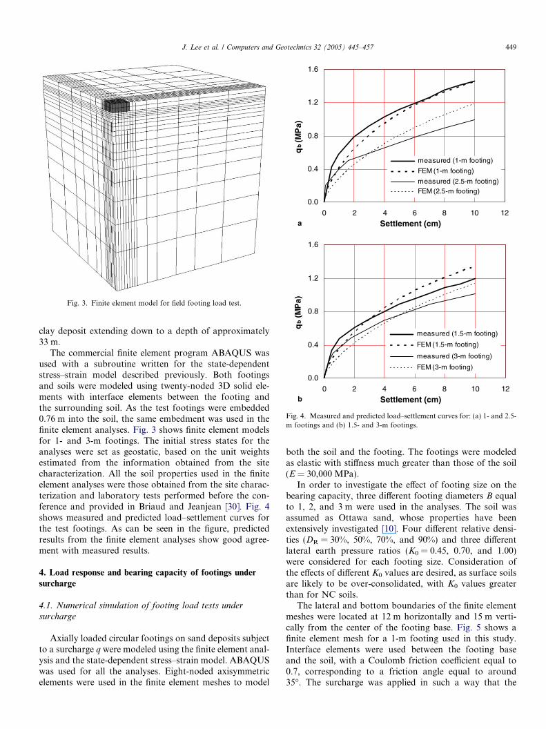
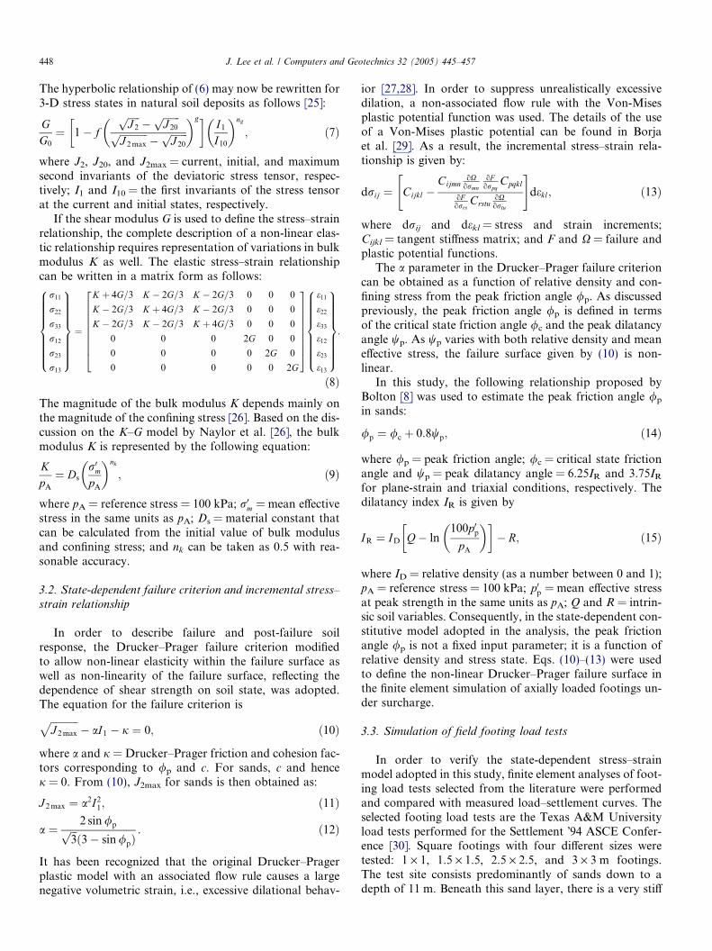
Fig. 3. Finite element model for field footing load test.

0.0

0.4

0.8

1.2

1.6

0 2 4 6 8 10

Settlement (cm)

qb

(MP

a)

measured (1-m footing)

FEM (1-m footing)

measured (2.5-m footing) FEM (2.5-m footing)

0.0

0.4

0.8

1.2

1.6

0 2 4 6 8 10

Settlement (cm)

qb (

MP

a)

measured (1.5-m footing)

FEM (1.5-m footing)

measured (3-m footing)

FEM (3-m footing)

12

12a

b

Fig. 4. Measured and predicted load–settlement curves for: (a) 1- and 2.5-m footings and (b) 1.5- and 3-m footings.

J. Lee et al. / Computers and Geotechnics 32 (2005) 445–457 449

clay deposit extending down to a depth of approximately33 m.

The commercial finite element program ABAQUS wasused with a subroutine written for the state-dependentstress–strain model described previously. Both footingsand soils were modeled using twenty-noded 3D solid ele-ments with interface elements between the footing andthe surrounding soil. As the test footings were embedded0.76 m into the soil, the same embedment was used in thefinite element analyses. Fig. 3 shows finite element modelsfor 1- and 3-m footings. The initial stress states for theanalyses were set as geostatic, based on the unit weightsestimated from the information obtained from the sitecharacterization. All the soil properties used in the finiteelement analyses were those obtained from the site charac-terization and laboratory tests performed before the con-ference and provided in Briaud and Jeanjean [30]. Fig. 4shows measured and predicted load–settlement curves forthe test footings. As can be seen in the figure, predictedresults from the finite element analyses show good agree-ment with measured results.

4. Load response and bearing capacity of footings under

surcharge

4.1. Numerical simulation of footing load tests under

surcharge

Axially loaded circular footings on sand deposits subjectto a surcharge q were modeled using the finite element anal-ysis and the state-dependent stress–strain model. ABAQUSwas used for all the analyses. Eight-noded axisymmetricelements were used in the finite element meshes to model

both the soil and the footing. The footings were modeledas elastic with stiffness much greater than those of the soil(E = 30,000 MPa).

In order to investigate the effect of footing size on thebearing capacity, three different footing diameters B equalto 1, 2, and 3 m were used in the analyses. The soil wasassumed as Ottawa sand, whose properties have beenextensively investigated [10]. Four different relative densi-ties (DR = 30%, 50%, 70%, and 90%) and three differentlateral earth pressure ratios (K0 = 0.45, 0.70, and 1.00)were considered for each footing size. Consideration ofthe effects of different K0 values are desired, as surface soilsare likely to be over-consolidated, with K0 values greaterthan for NC soils.

The lateral and bottom boundaries of the finite elementmeshes were located at 12 m horizontally and 15 m verti-cally from the center of the footing base. Fig. 5 shows afinite element mesh for a 1-m footing used in this study.Interface elements were used between the footing baseand the soil, with a Coulomb friction coefficient equal to0.7, corresponding to a friction angle equal to around35�. The surcharge was applied in such a way that the

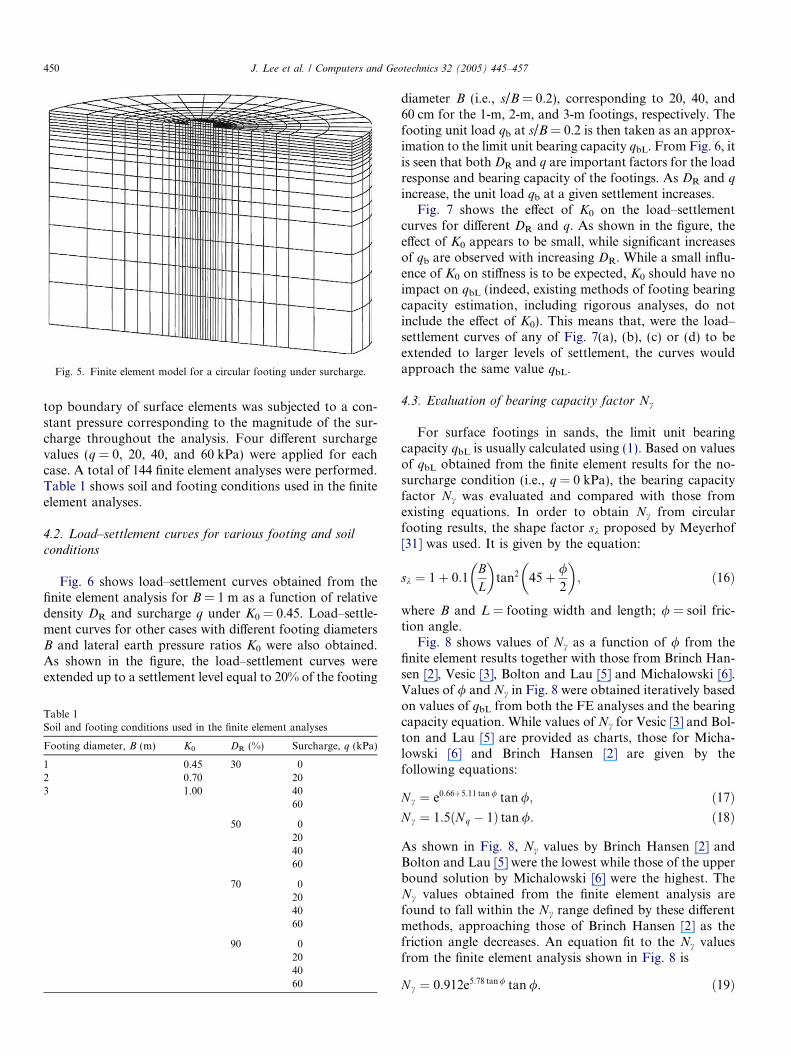
Fig. 5. Finite element model for a circular footing under surcharge.

450 J. Lee et al. / Computers and Geotechnics 32 (2005) 445–457

top boundary of surface elements was subjected to a con-stant pressure corresponding to the magnitude of the sur-charge throughout the analysis. Four different surchargevalues (q = 0, 20, 40, and 60 kPa) were applied for eachcase. A total of 144 finite element analyses were performed.Table 1 shows soil and footing conditions used in the finiteelement analyses.

4.2. Load–settlement curves for various footing and soil

conditions

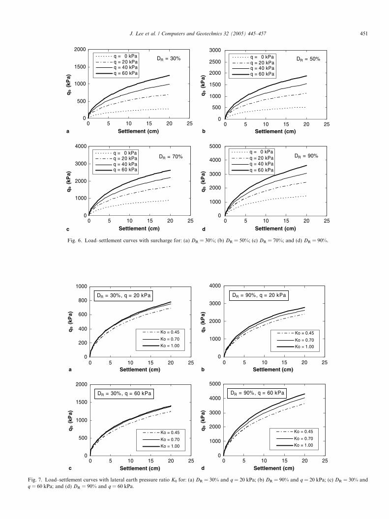
Fig. 6 shows load–settlement curves obtained from thefinite element analysis for B = 1 m as a function of relativedensity DR and surcharge q under K0 = 0.45. Load–settle-ment curves for other cases with different footing diametersB and lateral earth pressure ratios K0 were also obtained.As shown in the figure, the load–settlement curves wereextended up to a settlement level equal to 20% of the footing

Table 1Soil and footing conditions used in the finite element analyses

Footing diameter, B (m) K0 DR (%) Surcharge, q (kPa)

1 0.45 30 02 0.70 203 1.00 40

60

50 0204060

70 0204060

90 0204060

diameter B (i.e., s/B = 0.2), corresponding to 20, 40, and60 cm for the 1-m, 2-m, and 3-m footings, respectively. Thefooting unit load qb at s/B = 0.2 is then taken as an approx-imation to the limit unit bearing capacity qbL. From Fig. 6, itis seen that bothDR and q are important factors for the loadresponse and bearing capacity of the footings. As DR and qincrease, the unit load qb at a given settlement increases.

Fig. 7 shows the effect of K0 on the load–settlementcurves for different DR and q. As shown in the figure, theeffect of K0 appears to be small, while significant increasesof qb are observed with increasing DR. While a small influ-ence of K0 on stiffness is to be expected, K0 should have noimpact on qbL (indeed, existing methods of footing bearingcapacity estimation, including rigorous analyses, do notinclude the effect of K0). This means that, were the load–settlement curves of any of Fig. 7(a), (b), (c) or (d) to beextended to larger levels of settlement, the curves wouldapproach the same value qbL.

4.3. Evaluation of bearing capacity factor Nc

For surface footings in sands, the limit unit bearingcapacity qbL is usually calculated using (1). Based on valuesof qbL obtained from the finite element results for the no-surcharge condition (i.e., q = 0 kPa), the bearing capacityfactor Nc was evaluated and compared with those fromexisting equations. In order to obtain Nc from circularfooting results, the shape factor sk proposed by Meyerhof[31] was used. It is given by the equation:

sk ¼ 1þ 0:1BL

� �tan2 45þ /

2

� �; ð16Þ

where B and L = footing width and length; / = soil fric-tion angle.

Fig. 8 shows values of Nc as a function of / from thefinite element results together with those from Brinch Han-sen [2], Vesic [3], Bolton and Lau [5] and Michalowski [6].Values of / and Nc in Fig. 8 were obtained iteratively basedon values of qbL from both the FE analyses and the bearingcapacity equation. While values of Nc for Vesic [3] and Bol-ton and Lau [5] are provided as charts, those for Micha-lowski [6] and Brinch Hansen [2] are given by thefollowing equations:

N c ¼ e0:66þ5:11 tan/ tan/; ð17ÞN c ¼ 1:5ðNq � 1Þ tan/. ð18Þ

As shown in Fig. 8, Nc values by Brinch Hansen [2] andBolton and Lau [5] were the lowest while those of the upperbound solution by Michalowski [6] were the highest. TheNc values obtained from the finite element analysis arefound to fall within the Nc range defined by these differentmethods, approaching those of Brinch Hansen [2] as thefriction angle decreases. An equation fit to the Nc valuesfrom the finite element analysis shown in Fig. 8 is

N c ¼ 0:912e5:78 tan/ tan/. ð19Þ

20

15

10

0

500

00

00

00

0 5 10 15 20 25

Settlement (cm)

qb

(kP

a)

q = 0 kPaq = 20 kPaq = 40 kPaq = 60 kPa

0

1000

2000

3000

4000

5000

0 5 10 15 20 25

Settlement (cm)

qb

(kP

a)

q = 0 kPaq = 20 kPaq = 40 kPaq = 60 kPa

0

500

1000

1500

2000

2500

3000

0 5 10 15 20 25Settlement (cm)

qb

(kP

a)

q = 0 kPaq = 20 kPaq = 40 kPaq = 60 kPa

0

1000

2000

3000

4000

0 5 10 15 20 25

Settlement (cm)

qb

(kP

a)

q = 0 kPaq = 20 kPaq = 40 kPaq = 60 kPa

DR = 30%

DR = 90%DR = 70%

DR = 50%

a b

c d

Fig. 6. Load–settlement curves with surcharge for: (a) DR = 30%; (b) DR = 50%; (c) DR = 70%; and (d) DR = 90%.

0

200

400

600

800

1000

0 5 10 15 20 25Settlement (cm)

qb

(kP

a)

Ko = 0.45

Ko = 0.70

Ko = 1.00

0

1000

2000

3000

4000

0 5 10 15 20 25Settlement (cm)

qb

(kP

a)

Ko = 0.45

Ko = 0.70

Ko = 1.00

0

500

1000

1500

2000

0 5 10 15 20 25Settlement (cm)

qb

(kP

a)

Ko = 0.45

Ko = 0.70

Ko = 1.00

0

1000

2000

3000

4000

5000

0 5 10 15 20 25Settlement (cm)

qb

(kP

a)

Ko = 0.45

Ko = 0.70

Ko = 1.00

DR = 30%, q = 20 kPa DR = 90%, q = 20 kPa

DR = 30%, q = 60 kPa DR = 90%, q = 60 kPa

a b

c d

Fig. 7. Load–settlement curves with lateral earth pressure ratio K0 for: (a) DR = 30% and q = 20 kPa; (b) DR = 90% and q = 20 kPa; (c) DR = 30% andq = 60 kPa; and (d) DR = 90% and q = 60 kPa.

J. Lee et al. / Computers and Geotechnics 32 (2005) 445–457 451

0

30

60

90

120

150

30 33 36 39 42 45

φ (o)

Nγ

FE analysis Michalowski

Vesic Bolton and Lau (smooth)

Brinch Hansen

Fig. 8. Values of Nc with / for different methods.

0

1000

2000

3000

4000

5000

6000

0 20 40 60 8

Surcharge q (kPa)

qb

L (k

Pa)

Dr = 30%

Dr = 50%

Dr = 70%

Dr = 90%

0

1000

2000

3000

4000

5000

6000

0 20 40 60 8

Surcharge q (kPa)

qb

L (k

Pa)

Dr = 30%Dr = 50%Dr = 70%Dr = 90%

0

1000

2000

3000

4000

5000

6000

0 20 40 60

Surcharge q (kPa)

qb

L (k

Pa)

Dr = 30%Dr = 50%Dr = 70%Dr = 90%

B = 1 m

B = 3 m

B = 2 m

80

0

0a

b

c

Fig. 9. Values of limit unit bearing capacity qbL for (a) B = 1 m; (b)B = 2 m; and (c) B = 3 m.

452 J. Lee et al. / Computers and Geotechnics 32 (2005) 445–457

4.4. Variation of bearing capacity factors with surcharge

As the soil friction angle / varies with the stress state,values of both Nq and Nc for a given soil deposit are notconstant either, varying as a function of the mobilizedstress state associated with the footing size and the presenceof a surcharge. This makes it difficult to quantify individualvariations of Nq and Nc when a surcharge exists, for thebearing capacity represents a combined resistance withcontributions from both the Nq and Nc terms.

Fig. 9 shows values of the limit unit bearing capacity qbLas a function of the surcharge q for different relative densi-ties DR and footing diameters B under K0 = 0.45. As can beseen in the figure, values of qbL are not linearly propor-tional to q, which is in contrast with what the bearingcapacity equation postulates. In order to investigate theeffects of the surcharge on the bearing capacity factors, acombined bearing capacity factor Nq–c is introduced asfollows:

Nq–c ¼qbL

0:3cBþ q; ð20Þ

where Nq–c = combined bearing capacity factor; qbL = li-mit unit bearing capacity; c = soil unit weight; B = footingdiameter; q = surcharge.

While it would be possible to represent variation of foot-ing bearing capacity in terms of individual variations of Nq

and Nc, the factor Nq–c represents the variation of the bear-ing capacity more effectively, as it is given by a single value.The combined bearing capacity factor Nq–c has been usedfor investigating the validity of the superposition conceptfor the bearing capacity equation [5,7]. For a given footingsize, Nq–c with no surcharge (i.e., q = 0) represents Nc,while it approaches Nq as the surcharge increases and startspredominating over the self-weight term. Fig. 10 showshow values of Nq–c vary with q as a function of DR andB. Variation of Nq–c is more pronounced as DR increasesand B decreases, both of which are associated with increas-ing dilatancy in sands. As shown in the figure, the value ofNq–c is highest at q = 0, while it decreases with increasing

0

50

100

150

200

250

300

0 20 40 60 8Surcharge q (kPa)

Nq

-γ

B = 1 m

B = 2 m

B = 3 m

DR = 90%

DR = 70%

DR = 50%

DR = 30%

0

Fig. 10. Variation of combined bearing capacity factor Nq–c withsurcharge.

J. Lee et al. / Computers and Geotechnics 32 (2005) 445–457 453

surcharge, as the dilatancy is suppressed due to the increas-ing confining stress. It is also seen that the rate of decreaseof Nq–c becomes more significant with decreasing sur-charge, as the dilatancy index IR decreases with increasinglogarithm of the confining stress.

5. Normalized bearing capacity of footings on soil deposits

with a surcharge

5.1. Load–settlement response of footings on soil subject to a

surcharge

As discussed previously, the use of the bearing capacityequation is subjected to various uncertainties. A possibleway to reduce such uncertainties is direct use of in situ testresults, provided that a direct correlation to the footingbearing capacity is available. In the present study, theCPT cone resistance qc was adopted to evaluate the bearing

0

1

2

3

4

0

0.0 5.0 10.0 15.0 20.0

qc (MPa)

Dep

th (m

)

Dr = 30% Dr = 50% Dr = 70% Dr = 90%

0

1

2

3

4

.0 5.0 10.0 15.0 20.0

qc (MPa)

Dep

th (m

)

Dr = 30% Dr = 50% Dr = 70% Dr = 90%

q = 0 kPa

q = 40 kPa

a b

c d

Fig. 11. CPT cone resistance qc with depth for: (a) q = 0 k

capacity of footings. In order to obtain the footing bearingcapacity based on qc, load–settlement curves obtained fromthe finite element analysis were normalized and replotted interms of the normalized footing unit load qb/qc and the rel-ative settlement s/B.

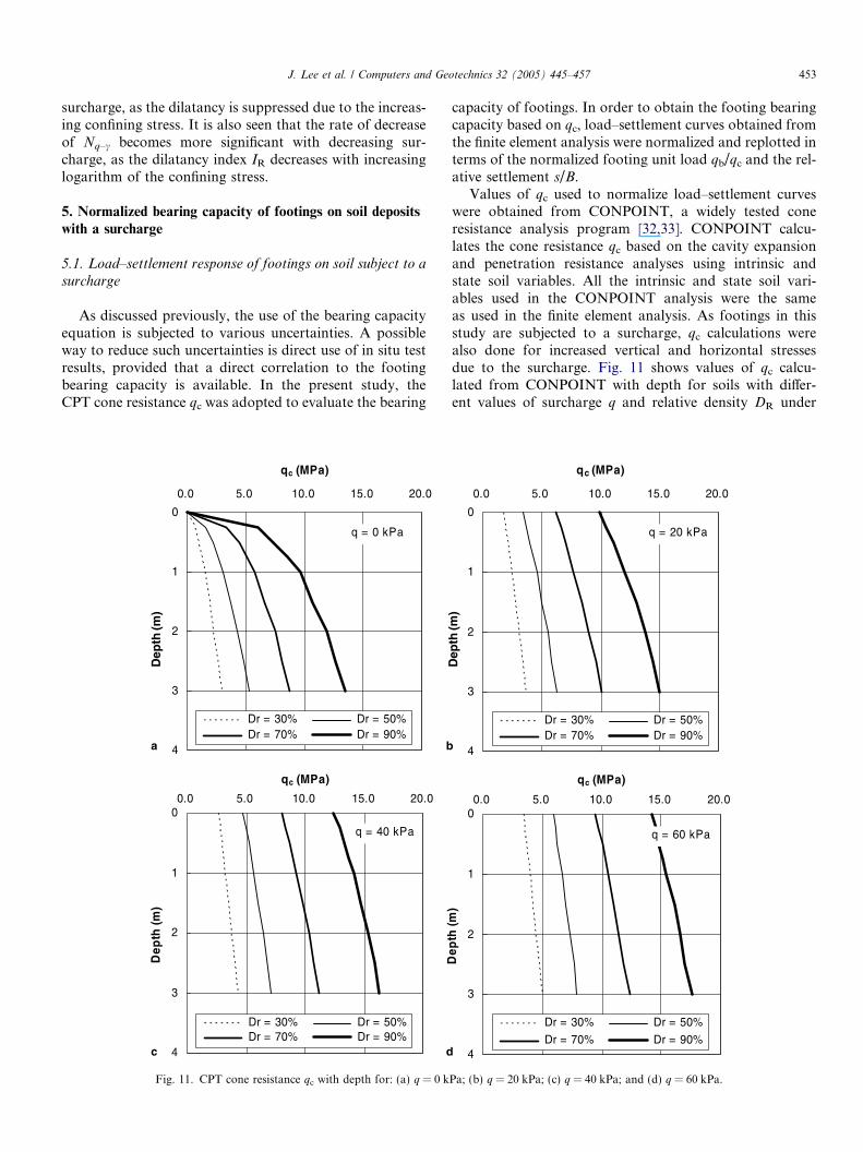
Values of qc used to normalize load–settlement curveswere obtained from CONPOINT, a widely tested coneresistance analysis program [32,33]. CONPOINT calcu-lates the cone resistance qc based on the cavity expansionand penetration resistance analyses using intrinsic andstate soil variables. All the intrinsic and state soil vari-ables used in the CONPOINT analysis were the sameas used in the finite element analysis. As footings in thisstudy are subjected to a surcharge, qc calculations werealso done for increased vertical and horizontal stressesdue to the surcharge. Fig. 11 shows values of qc calcu-lated from CONPOINT with depth for soils with differ-ent values of surcharge q and relative density DR under

0

1

2

3

4

0.0 5.0 10.0 15.0 20.0

qc (MPa)D

epth

(m)

Dr = 30% Dr = 50% Dr = 70% Dr = 90%

0

1

2

3

4

0.0 5.0 10.0 15.0 20.0

qc (MPa)

Dep

th (m

)

Dr = 30% Dr = 50%

Dr = 70% Dr = 90%

q = 20 kPa

q = 60 kPa

Pa; (b) q = 20 kPa; (c) q = 40 kPa; and (d) q = 60 kPa.

454 J. Lee et al. / Computers and Geotechnics 32 (2005) 445–457

K0 = 0.45. As described in Fig. 1, the slipline underneatha footing at failure is in general observed to extend to adepth, measured from the footing base, approximatelyequal to the footing diameter B. Accordingly, qc valuesused to normalize the load–settlement curves were aver-age cone resistances qc,avg from the footing base to adepth equal to B (corresponding to 1, 2, and 3 m forthe 1-, 2-, and 3-m footings, respectively) below the foot-ing base.

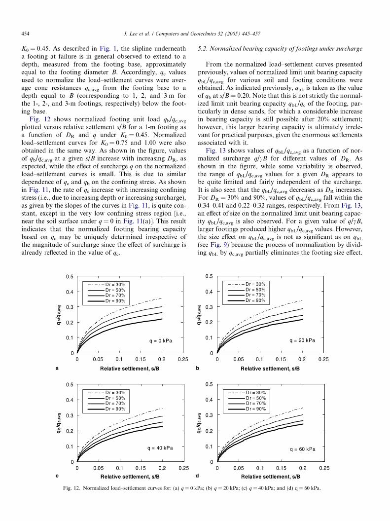
Fig. 12 shows normalized footing unit load qb/qc,avgplotted versus relative settlement s/B for a 1-m footing asa function of DR and q under K0 = 0.45. Normalizedload–settlement curves for K0 = 0.75 and 1.00 were alsoobtained in the same way. As shown in the figure, valuesof qb/qc,avg at a given s/B increase with increasing DR, asexpected, while the effect of surcharge q on the normalizedload–settlement curves is small. This is due to similardependence of qc and qb on the confining stress. As shownin Fig. 11, the rate of qc increase with increasing confiningstress (i.e., due to increasing depth or increasing surcharge),as given by the slopes of the curves in Fig. 11, is quite con-stant, except in the very low confining stress region [i.e.,near the soil surface under q = 0 in Fig. 11(a)]. This resultindicates that the normalized footing bearing capacitybased on qc may be uniquely determined irrespective ofthe magnitude of surcharge since the effect of surcharge isalready reflected in the value of qc.

0

0

0.1

0.2

0.3

0.4

0.5

0 0.05 0.1 0.15 0.2 0.25

Relative settlement, s/B

qb/q

c,av

g

Dr = 30%Dr = 50%Dr = 70%Dr = 90%

0.1

0.2

0.3

0.4

0.5

0 0.05 0.1 0.15 0.2 0.25

Relative settlement, s/B

qb/q

c,av

g

Dr = 30%Dr = 50%Dr = 70%Dr = 90%

q = 0 kPa

q = 40 kPa

a

c d

b

Fig. 12. Normalized load–settlement curves for: (a) q = 0 k

5.2. Normalized bearing capacity of footings under surcharge

From the normalized load–settlement curves presentedpreviously, values of normalized limit unit bearing capacityqbL/qc,avg for various soil and footing conditions wereobtained. As indicated previously, qbL is taken as the valueof qb at s/B = 0.20. Note that this is not strictly the normal-ized limit unit bearing capacity qbL/qc of the footing, par-ticularly in dense sands, for which a considerable increasein bearing capacity is still possible after 20% settlement;however, this larger bearing capacity is ultimately irrele-vant for practical purposes, given the enormous settlementsassociated with it.

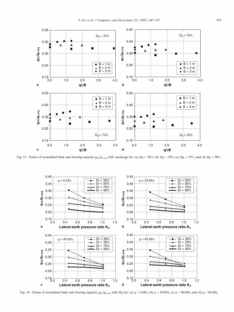
Fig. 13 shows values of qbL/qc,avg as a function of nor-malized surcharge q/cB for different values of DR. Asshown in the figure, while some variability is observed,the range of qbL/qc,avg values for a given DR appears tobe quite limited and fairly independent of the surcharge.It is also seen that the qbL/qc,avg decreases as DR increases.For DR = 30% and 90%, values of qbL/qc,avg fall within the0.34–0.41 and 0.22–0.32 ranges, respectively. From Fig. 13,an effect of size on the normalized limit unit bearing capac-ity qbL/qc,avg is also observed. For a given value of q/cB,larger footings produced higher qbL/qc,avg values. However,the size effect on qbL/qc,avg is not as significant as on qbL(see Fig. 9) because the process of normalization by divid-ing qbL by qc,avg partially eliminates the footing size effect.

0

0.1

0.2

0.3

0.4

0.5

0 0.05 0.1 0.15 0.2 0.25

Relative settlement, s/B

qb/q

c,av

g

Dr = 30%Dr = 50%Dr = 70%Dr = 90%

0

0.1

0.2

0.3

0.4

0.5

0 0.05 0.1 0.15 0.2 0.25

Relative settlement, s/B

qb/q

c,av

g

Dr = 30%Dr = 50%Dr = 70%Dr = 90%

q = 60 kPa

q = 20 kPa

Pa; (b) q = 20 kPa; (c) q = 40 kPa; and (d) q = 60 kPa.

0.10

0.20

0.30

0.40

0.50

0.0 1.0 2.0 3.0 4.0

q/γB

qb

L/q

c,av

g

B = 1 m B = 2 m B = 3 m

0.10

0.20

0.30

0.40

0.50

0.0 1.0 2.0 3.0 4.0

q/γB

qb

L/q

c,av

g

B = 1 mB = 2 mB = 3 m

0.10

0.20

0.30

0.40

0.50

0.0 1.0 2.0 3.0 4.0

q/γB

qb

L/q

c,av

g

B = 1 mB = 2 mB = 3 m

0.10

0.20

0.30

0.40

0.50

0.0 1.0 2.0 3.0 4.

q/γB

qb

L/q

c,av

g

B = 1 m B = 2 m B = 3 m

DR = 30% DR = 50%

DR = 70% DR = 90%

0

a b

c d

Fig. 13. Values of normalized limit unit bearing capacity qbL/qc,avg with surcharge for: (a) DR = 30%; (b) DR = 50%; (c) DR = 70%; and (d) DR = 90%.

0.

0.

0.

0.

0.

0.

0.

0.

0.

0.

0.

0.

0.

0.

15

20

25

30

35

40

45

0.2 0.4 0.6 0.8 1.0 1.2

Lateral earth pressure ratio K0

qb

L/q

c,av

g

Dr = 30% Dr = 50% Dr = 70% Dr = 90%

0.15

0.20

0.25

0.30

0.35

0.40

0.45

0.2 0.4 0.6 0.8 1.0 1.2

Lateral earth pressure ratio K0

qb

L/q

c,av

g

Dr = 30% Dr = 50% Dr = 70% Dr = 90%

15

20

25

30

35

40

45

0.2 0.4 0.6 0.8 1.0 1.2Lateral earth pressure ratio K0

qb

L/q

c,av

g

Dr = 30% Dr = 50% Dr = 70% Dr = 90%

0.15

0.20

0.25

0.30

0.35

0.40

0.45

0.2 0.4 0.6 0.8 1.0 1.2Lateral earth pressure ratio K0

qb

L/q

c,av

g

Dr = 30%Dr = 50%Dr = 70%Dr = 90%

q = 0 kPa q = 20 kPa

q = 40 kPa q = 60 kPa

a b

c d

Fig. 14. Values of normalized limit unit bearing capacity qbL/qc,avg with DR for: (a) q = 0 kPa; (b) q = 20 kPa; (c) q = 40 kPa; and (d) q = 60 kPa.

J. Lee et al. / Computers and Geotechnics 32 (2005) 445–457 455

456 J. Lee et al. / Computers and Geotechnics 32 (2005) 445–457

This is because the larger the footing size, the deeper theinfluence zone used for the determination of qc,avg is. Asthe footing size effect is primarily related to reduction ofthe soil friction angle with increasing depth, the determina-tion of qc,avg is itself a way to capture some of this footingsize effect.

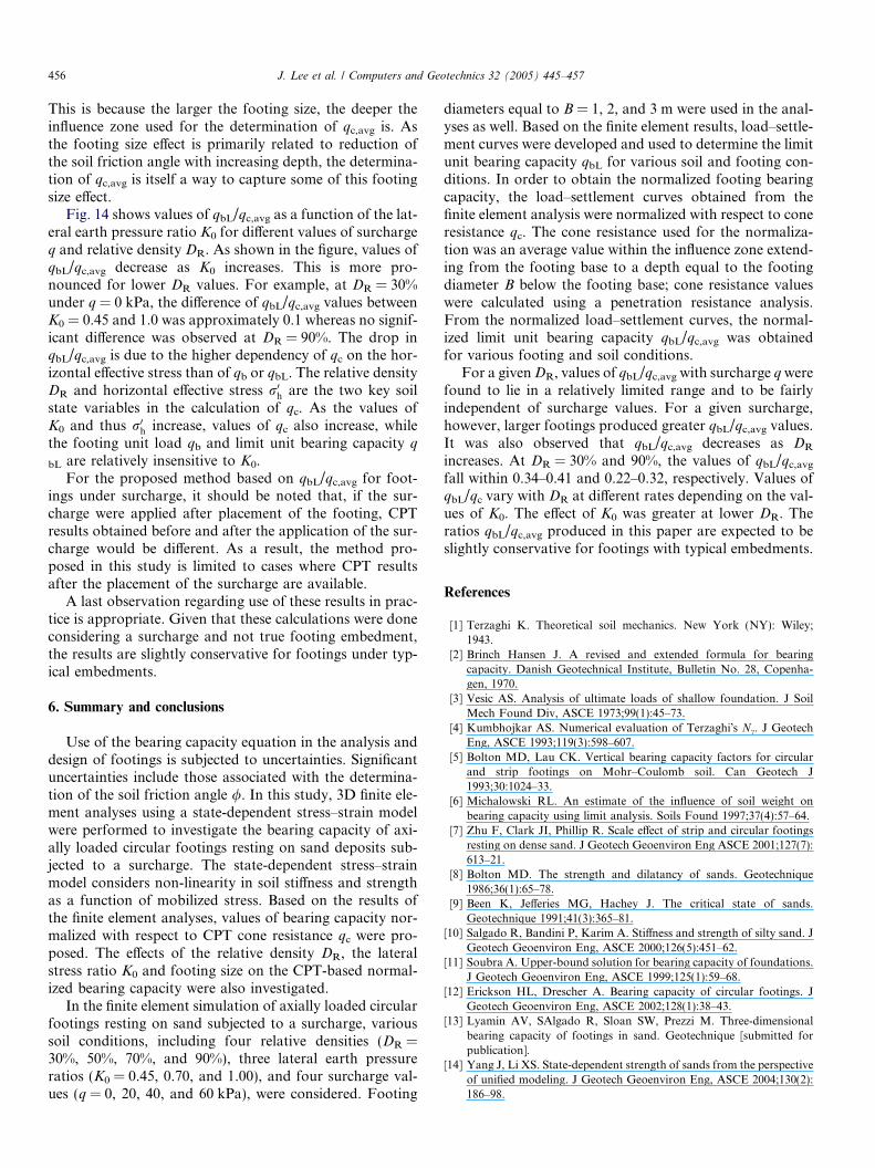
Fig. 14 shows values of qbL/qc,avg as a function of the lat-eral earth pressure ratio K0 for different values of surchargeq and relative density DR. As shown in the figure, values ofqbL/qc,avg decrease as K0 increases. This is more pro-nounced for lower DR values. For example, at DR = 30%under q = 0 kPa, the difference of qbL/qc,avg values betweenK0 = 0.45 and 1.0 was approximately 0.1 whereas no signif-icant difference was observed at DR = 90%. The drop inqbL/qc,avg is due to the higher dependency of qc on the hor-izontal effective stress than of qb or qbL. The relative densityDR and horizontal effective stress r0

h are the two key soilstate variables in the calculation of qc. As the values ofK0 and thus r0

h increase, values of qc also increase, whilethe footing unit load qb and limit unit bearing capacity q

bL are relatively insensitive to K0.For the proposed method based on qbL/qc,avg for foot-

ings under surcharge, it should be noted that, if the sur-charge were applied after placement of the footing, CPTresults obtained before and after the application of the sur-charge would be different. As a result, the method pro-posed in this study is limited to cases where CPT resultsafter the placement of the surcharge are available.

A last observation regarding use of these results in prac-tice is appropriate. Given that these calculations were doneconsidering a surcharge and not true footing embedment,the results are slightly conservative for footings under typ-ical embedments.

6. Summary and conclusions

Use of the bearing capacity equation in the analysis anddesign of footings is subjected to uncertainties. Significantuncertainties include those associated with the determina-tion of the soil friction angle /. In this study, 3D finite ele-ment analyses using a state-dependent stress–strain modelwere performed to investigate the bearing capacity of axi-ally loaded circular footings resting on sand deposits sub-jected to a surcharge. The state-dependent stress–strainmodel considers non-linearity in soil stiffness and strengthas a function of mobilized stress. Based on the results ofthe finite element analyses, values of bearing capacity nor-malized with respect to CPT cone resistance qc were pro-posed. The effects of the relative density DR, the lateralstress ratio K0 and footing size on the CPT-based normal-ized bearing capacity were also investigated.

In the finite element simulation of axially loaded circularfootings resting on sand subjected to a surcharge, varioussoil conditions, including four relative densities (DR =30%, 50%, 70%, and 90%), three lateral earth pressureratios (K0 = 0.45, 0.70, and 1.00), and four surcharge val-ues (q = 0, 20, 40, and 60 kPa), were considered. Footing

diameters equal to B = 1, 2, and 3 m were used in the anal-yses as well. Based on the finite element results, load–settle-ment curves were developed and used to determine the limitunit bearing capacity qbL for various soil and footing con-ditions. In order to obtain the normalized footing bearingcapacity, the load–settlement curves obtained from thefinite element analysis were normalized with respect to coneresistance qc. The cone resistance used for the normaliza-tion was an average value within the influence zone extend-ing from the footing base to a depth equal to the footingdiameter B below the footing base; cone resistance valueswere calculated using a penetration resistance analysis.From the normalized load–settlement curves, the normal-ized limit unit bearing capacity qbL/qc,avg was obtainedfor various footing and soil conditions.

For a givenDR, values of qbL/qc,avg with surcharge qwerefound to lie in a relatively limited range and to be fairlyindependent of surcharge values. For a given surcharge,however, larger footings produced greater qbL/qc,avg values.It was also observed that qbL/qc,avg decreases as DR

increases. At DR = 30% and 90%, the values of qbL/qc,avgfall within 0.34–0.41 and 0.22–0.32, respectively. Values ofqbL/qc vary with DR at different rates depending on the val-ues of K0. The effect of K0 was greater at lower DR. Theratios qbL/qc,avg produced in this paper are expected to beslightly conservative for footings with typical embedments.

References

[1] Terzaghi K. Theoretical soil mechanics. New York (NY): Wiley;1943.

[2] Brinch Hansen J. A revised and extended formula for bearingcapacity. Danish Geotechnical Institute, Bulletin No. 28, Copenha-gen, 1970.

[3] Vesic AS. Analysis of ultimate loads of shallow foundation. J SoilMech Found Div, ASCE 1973;99(1):45–73.

[4] Kumbhojkar AS. Numerical evaluation of Terzaghi�s Nc. J GeotechEng, ASCE 1993;119(3):598–607.

[5] Bolton MD, Lau CK. Vertical bearing capacity factors for circularand strip footings on Mohr–Coulomb soil. Can Geotech J1993;30:1024–33.

[6] Michalowski RL. An estimate of the influence of soil weight onbearing capacity using limit analysis. Soils Found 1997;37(4):57–64.

[7] Zhu F, Clark JI, Phillip R. Scale effect of strip and circular footingsresting on dense sand. J Geotech Geoenviron Eng ASCE 2001;127(7):613–21.

[8] Bolton MD. The strength and dilatancy of sands. Geotechnique1986;36(1):65–78.

[9] Been K, Jefferies MG, Hachey J. The critical state of sands.Geotechnique 1991;41(3):365–81.

[10] Salgado R, Bandini P, Karim A. Stiffness and strength of silty sand. JGeotech Geoenviron Eng, ASCE 2000;126(5):451–62.

[11] Soubra A. Upper-bound solution for bearing capacity of foundations.J Geotech Geoenviron Eng, ASCE 1999;125(1):59–68.

[12] Erickson HL, Drescher A. Bearing capacity of circular footings. JGeotech Geoenviron Eng, ASCE 2002;128(1):38–43.

[13] Lyamin AV, SAlgado R, Sloan SW, Prezzi M. Three-dimensionalbearing capacity of footings in sand. Geotechnique [submitted forpublication].

[14] Yang J, Li XS. State-dependent strength of sands from the perspectiveof unified modeling. J Geotech Geoenviron Eng, ASCE 2004;130(2):186–98.

J. Lee et al. / Computers and Geotechnics 32 (2005) 445–457 457

[15] Kondner RL. Hyperbolic stress–strain response: cohesive soil. J SoilMech Found Eng Div, ASCE 1963;189(SM1):115–43.

[16] Duncan JM, Chang CY. Nonlinear analysis of stress–strain in soils. JSoil Mech Found Eng Div, ASCE 1970;96(SM5):1629–53.

[17] Hardin BO, Drnevich VP. Shear modulus and damping in soils;design equations and curves. J Soil Mech Found Div, ASCE1972;98(7):667–92.

[18] Tatsuoka F, Siddiquee MSA, Park C, Sakamoto M, Abe F. Modelingstress–strain relations in sand. Soils Found 1993;33(2):60–81.

[19] Fahey M, Carter JP. A finite element study of the pressuremeter testin sand using a non-linear elastic–plastic model. Can Geotech J1993;30(2):348–61.

[20] Yu P, Richart FE. Stress ratio effects on shear modulus of dry sands.J Geotech Eng, ASCE 1984;110:331–45.

[21] Viggiani G, Atkinson JH. Interpretation of bender element tests.Geotechnique 1995;45(1):149–54.

[22] Salgado R, Mitchell JK, Jamiolkowski M. Cavity expansion andpenetration resistance in sand. J Geotech Geoenviron Eng, ASCE1997;123(4):344–54.

[23] Hardin BO, Black WL. Sand stiffness under various triaxial stresses.J Soil Mech Found Eng Div, ASCE 1966;92(SM2):27–42.

[24] Teachavorasinskun S, Shibuya S, Tatsuoka F. Stiffness of sandsin monotonic and cyclic torsional simple shear. Proc Geotech

Eng Congr, Geotechnical Special Publication, ASCE 1991;1(27):863–78.

[25] Lee JH, Salgado R. Analysis of calibration chamber plate load tests.Can Geotech J 2000;37(1):14–25.

[26] Naylor DJ, Pande GN, Simpson B, Tabb R. Finite elements ingeotechnical engineering. Swansea, Wales, UK: Pineridge Press; 1981.

[27] Desai CS, Siriwardane HJ. Constitutive laws for engineering mate-rials with emphasis on geologic material. Englewood Cliffs: Prentice-Hall; 1984.

[28] Chen WF, Baladi GY. Soil plasticity; theory and implementation.New York: Elsevier Science Publishing Company Inc.; 1985.

[29] Borja RI, Lee SR, Seed RB. Numerical simulation of excavation inelastoplastic soils. Int J Numer Anal Methods Geomech 1989;13(3):231–49.

[30] Briaud JL, Jeanjean P. Load–settlement curve method for spreadfootings on sand. In: Proceedings of settlement �94, vertical andhorizontal deformations of foundations and embankments, ASCE,vol. 2; 1994. p. 1774–804.

[31] Meyerhof GG. Some recent research on the bearing capacity offoundations. Can Geotech J 1963;1(1):16–26.

[32] Salgado R, Randolph MF. Analysis of cavity expansion in sands. IntJ Geomech 2001;1(2):175–92.

[33] Salgado R. CONPOINT MANUAL. 2003.