hydrodynamic thrust bearing study

HYDRODYNAMIC THRUST BEARING STUDY

BY

Christopher Miles McCulloch Ettles

A thesis submitted for the degree of

DOCTOR OF PHILOSOPHY

of the

University of London

and 'also for the

DIPLOMA OF IMPERIAL COLLEGE

July, 1965

Mechanical Engineering Department, Imperial College, London, S. W. 7.

-1-

ABSTZACT

The pressure generation of parallel surface bearings

has been investigated experimentally using dynamic instru-

mentation mounted in the moving surface. It was found that

when the pads were truly flat and parallel a negative pressure

was generated which was approximately proportional to the

inverse square of film thickness.

A complete reversal of pressure generation was

shown as the film thickness was successively decreased. This

is shown to be due to increasing thermal distortion of the

pads. It is shown that useful loads are carried on a

wedge shaped film produced by thermal distortion.

Appropriate theory has been developed for the

infinitely wide case which includes the density and viscosity

wedge effects, variations of film shape, frictional genera-

tion and conduction to the bearing solids. Fair agreement

was obtained between theory and experiment after suitable

treatment for side leakage.

The problem of transfer of heat and velocity

across the bearing groove has been studied. This phenomenon

has been shown to exert a strong influence on bearing

performance.

-2-

ACKNOWLEDGEMENTS

I should like to offer my particular thanks to the following:-

To Dr. A. Cameron, my supervisor, for his continual sound

advice.

To Joseph Lucas Industries Ltd., for generous financial and

technical assistance, and to many of the staff of this

company for their advice and help.

To the Department of Scientific and Industrial Research for

a Research Studentship grant.

-3-

LIST OF CONTENTS

Abstract 1 Acknowledgements 2

List of Contents 3

List of Figures 6

Chapter 1 •

1.1. Introduction 12

1.2. Literature survey 13

1.3. Nomenclature 22

Chapter 2. Initial Theory

2.1. The viscosity wedge 24

2.2. The thermal wedge 29

2.3. Comparison of mechanisms 30

Chapter 3. Apparatus

3.1. Requirements 32

3.2. Measurement of rotor surface temperature 33

3.3. Measurement of film thickness 40

3.4. Measurement of film pressure 41

3.6. First testbearing 45

3.6. Test rig 47

3.7. Calibration 56

3.8. Test procedure 61

Chapter 4. Experimental Results

4.1. Pressure transducer outputs 72

4.2. Analysis of wedge size 85

4.3. Measurement of boundary inlet pressure 91

4.4. Measurement of parallel surface

pressure generation 94

4.5. Comment on results 103

-4-

LIST OF CONTENTS

Chapter 5. Theory

5.1. Requirements and assumptions 110

5.2. Frictional generation 112

5.3. Theoretical results ' 113

5.4. Treatment for side leakage 116 5.5. Agreement of theory and experiment 120

Chapter 6. Mass and Heat Flow in the Bearing Groove

6.1. General

6.2. Boundary layer formation

127

127

6.3. Thermal effects in boundary layer 131 6.4. Varying viscosity boundary layer 132 6.5. Comment on leading edge ram results 135 6.6. Hot oil carry-over 138 6.7. Comment on results of heat carried over • • 139

Chapter 7. Second Test Series

7.1. Procedure 146

7.2. Results 146

7.3. Comment on experimental results 159

7.4. Theory 163

7.5. Practical Implications of results 177

Chapter 8. Conclusions 180 APPENDICES

Appendix 1. Bibliography 186 Appendix 2. • .• 4, 4., •• •1, • •. • Initial theOry , Appendix 2.1. Setting up 190 Appendix 2.2. Integration of (A2.9) 193 Appendix 3.

A3.1. Test oil data 198

-5-

A3.2. Pressure transducer calibration 200

A3.3. Capacitance gauges calibration 201

A3.4. Rotor thermocouple calibration 204

Appendix 4. Theory

A4.1. Setting up 205

A4.2. Frictional generation and conduction 209

A4.3. Solution 214

A4.4. Computer programme 216

Appendix 5. Heat and mass transfer in groove

A5.1. Solution of varying viscosity boundary

layer 220

A5.2. Thickness of varying viscosity boundary

layer 223

A5.3. Velocity ram pressure 224

A5.4. Viscous ram pressure in 45° chamfer 226

A5.5. Hot oil carry over 227

Appendix 6. Analysis of pad distortion

A6.1. Thermal bending 232

A6.2. The effect of asymmetrical temperature

distribution 235

A6.3. Direct expansion 238

-fi-

LIST OF FIGURES AND TABLES

2.1. Temperature distributions 24

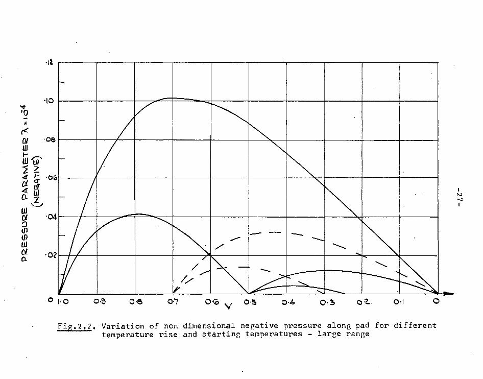
2.2. Variation of non-dimensional pressure large range 27

2.3. /I It It - small range 28

3.1. Conductive lubricant thermocouple 34k

3.2. Output of 3.1 34

3.3. Surface thermocouple 35

3.4. Capacitance probe 41

3.5. Pressure sensitive bolt 42 3.6. Piezo electric pressure transducer 43

3.7. Rotor ' 44

3.8. Rotor 44

3.9. First test bearing 46

3.10. Test housing and shaft 48

3.11. View of test housing and shaft 50 3.12. View of test housing and shaft 50 3.13. Hydraulic circuit 52 3.14. General view of test machine 53

3.15. Recording equipment 53

3.16. Calibration bearing 56

3.17. Effect of bearing high spot 59

3.18. Firstspecimen test record . . . -.....-......-...-. 62

3.19. Specimen oscillograms. Test 4J 65 3.20. li II II Test 81 66 3.21. II II Test 5N 68,69

3.22. n Test 26P 70

3.23. Pressure developed in'first test series . 64

3.24. Modifications to bearing 63

-7-


Table 4.1. Experimental readings 73,74

4.1. Pad Temperature 75,76

4.2. Typical pressure transducer output 72

4.3.(a) Analysis of pressure transducer

output 81

(b) Crystal surface elemental areas 81

Table 4.2. Sample numerical analysis 80

4.4. Observed and true pressure curves 83

for a circular transducer with

D/rc = 0.8

4.5. Variation of attenuation ratio with D/rc 85

4.6.(a) Analysis of capacitance trace 87

(b) Integration of capacitance 87

4.7. Evaluation of wedge amplitude 89

4.8. Model for evaluation of capacitance side 90

leakages

4.9. Change in flux lines due to presence 90

of chamfered edge

4.10. Correction for side leakage 89

4.11. Position of D relative to end of

Amax

internal wedge 93

4.12. Measurement from transducer outputs 93

4.13. Analogue for the solution ofpbouridary

pressure field 95

4.14a, b. Measurement of parallel surface 97,98

pressure generation

4.15. Parallel surface pressure generation 99

960 RPM.

-8-


4.16.

4.17.

Parallel surface pressure generation 1610 11 11 II 11 2180

RPM

RPM

100

101

4.18. " It it . it ri 3670 RPM 102

4.19. Effect of pad temperature profile 103

4.20. Effect of three dimensional pad

temperature 105

4.21. Effect of decreasing film thickness 106

4.22. Idealised temperature distribution 107

5.1. Film temperature 110

5.2. Computer solutions for temperature and

pressure 114

5.3. Effect of trailing edge temperature drop. 115

5.4. Effect of conduction to bearing solids 115

5.5. Shape and mesh size of analysed area 118

5.6. Hypothetical dimensionless film thickness 118

5.7. Dimensionless pressure 118

5.8. Variation of side leakage factor along

radius p3 117

5.9. Correlation between theory and

experiment 960 RPM 122


experiment 1610 RPM 12.3,124





-9-


6.1. Adoption of standard boundary layer

profile 128

6.2. Propagation of an exit profile by

Wittings method 130

6.3. Formation of thermal boundary layer 131

6.4. Assumed variation of viscosity through

thermal layer 133

6.5. Comparison of isoviscous and non-iso-

viscous velocity profiles 133

6.6. Effect of viscosity profile and viscosity ratio on boundary layer .... 134

Table 6.1. Theoretical and experimental

correlation 136

Table 6.2. of leading edge pressures 137

6.7. Effect of speed and film thickness on

hot oil carry over

Groove width: 0.145 inches 142

6.8. (Same). Groove width: 1.58 inches 143

6.9. Cooling fins on rotor 145

Tables 7.1. General test data

7.2. General test data

7.1. Test bearing with three pads

7.2. (Same)

7.3. Pad temperature distribution

1610 RPM

7.4. Pad temperature distribution

3670 RPM. 151

7.5. Pressure transducer output 960 RPM 152,153

removed .

960 and

1610 and

147

148

149

149

150

-10-

LIST OF FIGURES AND TABLES 155

156

157

7.6.

7.7.

7.8.

Pressure transducer output 1610 RPM II II 11 2180 RPM n n n 3670 RPM

7.9. Pressure generation with boundary field

subtracted 1610 RPM 158

7.10. p2 and p3 transducer outputs 160

7.11. Correlation of theoretical and measured

distortion 162

7.12. Distorted bearing shape 164

7.13. Functions for temperature variation

along pad 166

7.14. Specimen computer results 168,169

7.15. Hypothetical film shape 171

7.16. Side leakage factor 171

7.17. Correlation of theory and experiment 960 RPM 174

7.18. 11 1610 RPM 175

7.19. IT 11 11 2180 RPM 176

7./0. Distortion of tongue type bearing 177

7.21. Insulation of trailing edge 178

-11-

APPENDICES

A2.1.

Table

Temperature distribution

A.1. Values of M/(J,1/ and

integrals

190

196,197

A3.1. Test oil data 198,199 A3.2. Pressure transducer calibration 200 A3.3. Capacitance gauge calibration 201

A3.4. Rotor thermocouple calibration 204

A4.1. Film temperatures 205

A4.2. Film temperature profile 206

A5.1. Axes for boundary layer 220

A5.2. Deflection of boundary layer 224

A5.3. Distribution of velocity and temper-

atures in groove 227

A5.4. Functions of t = 0:-(y/ b t)i 228

A5.5. Comparison of standard velocity

profiles 228

A5.6. Solution of thermal layer equation 230

A6.1. Thermal bending of circular pad and

backing 232

A6.2. Case for asymmetrical temperature

distribution 236

A6.3. Differing distortion with symmet-

rical and asymmetrical temperat-

ure distribution 237

-12-

CHAPTER 1

1.1. Introduction

Of the various types of hydrodynamic thrust bearing,

the parallel surfacc bearing has been of both practical and

academic interest for many years. The original equations of

Osborne Reynolds inherently specify a converging film for

load carrying capacity. The parallel surface bearing ipso

facto should have no load carrying capacity. Yet this

bearing has been in use since the last century.

The use of the parallel surface bearing long pre-

ceded any research as to its mode of action. For many years

the multiple collar thrust bearing was in use for marine

thrust blocks and for taking up thrust in gear trains. Design was on an arbitrary basis of 50-60 psi. This

bearing was superseded in 1905 by Michell's tilting pad bear-

ing although the parallel surface bearing continued to be

used for many years in marine applications.

The parallel surface bearing remains in use today

for many smaller applications due to its simplicity of

manufacture, yet the mechanism of load carrying remains

unclear. "Six theories have been put forward in past

literature as to this mechanism. These are described

in the next section but may be listed as

1. Fogg, Thermal expansion of lubricant

2. Swift, Thermal expansion of bearing

3. Salama, Long-wave indulations of bearing surface

4. Cameron, The "viscosity" wedge.

J. Lewicki, Leading edge ram pressure.

6. Harrison, Chamfer at edge.

Recent work by Dowson and Hudson (23) showed that

the parallel surface bearing should generate a negative load

-13-

The work described in this thesis was undertaken

to investigate the mode of action of the parallel surface

bearing and to correlate results with new or existing theory.

1.2. Literature survey

The parallel surface bearing was first described by Beauchamp Tower (33) in 1891.

Two contributors to the discussion of a paper bv.

Newbigin (1) 1914 described improvements they had carried

out on the multiple collar thrust bearing. de Ferranti

found that a pressure of 500 p.s.i. could be carried on

multiple collar bearing at moderate speeds if there was

equal load sharing using a spring system. Loads of up to

1000 p.s.i. could be carried after cutting "deep" Oooves

in the face of the bearing. Gibson reported a similar

improvement in a marine thrust block after the cutting of

seven large radial grooves in the face of the originally

plane horse shoe type bearing.

In 1919 Harrison (34) suggested that pressure was

generated by chamfer on the pad edges, but gave no quantitative

data to support this.

In 1946 Fogg (2) reported his now classical

experiments on parallel thrust surfaces. Fogg found that

plairwrings had a very poor load carrying capacity and cut

two small sharp edge radial grooves to improve oil flow

to the bearing. An unexpectedly high load carrying

capacity resulted which was comparable to Michell pads.

Very high rotative speeds were used. Fogg used sharp

edged grooves to reduce any taper effect at the leading

edge, but found later that radiused grooves had no effect

on performance. Fogg gave a tentative theory that load

was carried by thermal expansion of the lubricant in the

film, showing that a 100°C rise through the film would be

equivalent to a 10% taper.

-14-

It is worth noting that Fogg later measured the

temperature distribution in the pads and found less than

3°C rise circumferentially. He also found that throttling

of the radial grooves at the outer edge was essential.,

to good bearing performance although the pressurisation

contributed negligibly to load carrying.

In the discussion to this paper Swift made the

first suggestion that load was carried by thermal distortion

of the bearing -Co form a wedge. Fogg discounted this

explanation since the bearing immediately supported a re-

applied load. Bower(disc.) reviewed the leading chamfer concept.

Cameron and Wood (3) gave the first quantitative

treatment of Fogg's "thermal wedge" theory, assuming the heat

conducted through the bearing solids was negligible and

that the temperature was constant across the film. Viscosity

and hence heat generation and expansipn were allowed to vary

with length, giving an asymmetric pressure distribution with

the maximum pressure towards the leading edge. In 1947

Shaw (4) gave a less advanced treatment of the thermal

wedge, using a linear temperature rise. He found that

approximately 10% of the equivalent Michell load could be

carried provided the film temperature rise was sufficiently

clear.

A similar result was found by Cope (5) in 1949.

Cope reduced the Navier Stokes equations by omitting various

terms thought to be negligible in hydrodynamic lubrication.

He nevertheless neglected change of lubricant properties

across the film. Cope fonnd that a high load could be

carried by the thermal wedge mechanism provided that

-15-

(1) There was a small variation of viscosity with temperature

(2) The lubricant had a high coefficient of cubical

expansion

(3) The film thickness was small.

A similar analysis was presented by Charnes, Osterle

and Saibel (6) in 1952. In 1953 they re-derived the energy

equation to include the flow work terms (7).

In 1950 Selma (8) discounted Fogg's and Swift's

explanations as secondary effects. He presented a theory

of load carrying as a result of long-wave undulations

(macro-roughness) produced by machining of the surfaces.

Salama assumed cavitation in the diverging portions of

the film and applied similar boundary conditions to those

used for journal bearings. He was able to obtain correlation

of theory and experiment using carefully produced wave-

forms on the bearing surface. Salami's theory failed to

explain the operation of flat lapped bearings which he

attributed initially to micro-roughness. He concluded

that the function of radial grooves was only to supply lub-

ricant and to cool the bearing surfaces.

In 1951 Cameron (9) considered the effect of

variation of viscosit52, across the lubricant film for contra-

rotating discs. He showed that if there was also a

temperature gradient in the direction of motion, a load could

be carried. In 1958 he applied a similar treatment to the

parallel surface thrust bearing (10). Cameron assumed that

the bearing was at constant temperature (corresponding to

Fogg's experimental finding (2)) and that the surface

-16-

temperature of the rotor rose along the film. A linear

temperature profile through the film was assumed. Cameron

found that with such a viscosity distribution in the film-

a load could be carried, and coined the term "viscosity

wedge". He showed that the viscosity wedge was more

powerful than the thermal wedge mechanism.

(In a subsequent treatment (21) in 1960, Cameron

showed that negative pressures were more likely. This is

described later).

In 1955 Lewicki (11) gave an analysis for the

generation of pressure at the leading edge of a slider from

the viscous ram effect. He attributed the lift of parallel

surface bearings to this pressure effect at the leading

edge. In 1957 he computed the effect of leading edge ram

on the conventional inclined plane bearing (12). From

Lewicki's theory, the pressure in a parallel slider should be

maximum at the leading edge and attenuate to slightly less

than zero at the trailing edge.

This was shown to be untrue in a well conducted

series of experiments by Kettleborough (13) in 1955, who

gave the first measurements of film pressure in the

parallel surface bearing. Kettleborough used a steel ring

bearing (4k" outer diameter, 24" internal diameter) divided

up into a number of segments by grooves 3/16" wide by au

deep. Loading was limited to 130 p.s.i. The number of

grooves was varied from 0, 2, 3, 4, 5, 6. Kettleborough

found that four grooves gave the best results in terms of

film thickness and friction. Tests were carried out at

a moderately slow speed but performance was found to

improve at a higher speed. Kettleborough found that although

pad temperature was much greater than the bulk oil temperature,

circumferential variation in temperature was low. This

-17-

confirmed Fogg's result(2). Film pressuresin the four pad

bearing were measured from six tapping holes in each of four

pads. The attainment of equilibrium of the pressure gauge

was very slow. Kettleborough found that, in spite of care-

ful lapping, the pressure generated varied widely from point to point due to local surface irregularities.

The explanation of the results in terms of the

thermal wedge was qualitative„ since the actual temperature

rise through the film was unknown although the pad temperature

rise was "not significant".

In 1957 Hunter and Zienkiewicz (14) considered the

effect of variation of temperature through the thickness of

the film. The two dimensional energy equation was used

to calculate the temperature in a parallel film, with itera-

tion between the velocity and temperature profiles until

equilibrium had been reached. Two examples were evaluated,

both with the boundary plates at constant temperature.

(Cameron (10) had previously considered a rising rotor

temperature with a linear temperature profile in the film).

In the first example both boundary plates were

maintained at the same temperature as the incoming oil.

An overall positive pressure generation was found with a

negative loop near the leading edge. In the second

example the moving boundary was maintained at a constant • ecual

temperature approximatelyATO the mean temperature of the oil

between the plates. The static boundary was maintained at

the oncoming oil temperature. With these modifications the

pressure generation was wholly positive. The effect of

neglecting density variation was found to be small. In.

-18-

1960 Hunter and Zienkiewicz continued this work to consider

the effect of temperature variation across converging

films (15).

Two examples were considered. In case (a) the

bearing temperatures were allowed to vary but the film was assumed adiabatic and the condition 11'/ y = 0 applied to at both surfaces. A somewhat unrealistic temperature

distribution resulted showing that this condition was un-

likely in practice. In case (b) this condition was dis-

carded and both solids were maintained at a constant

temperature equal to that of the oncoming oil. Both cases

gave lower pressures than the solution which allowed

variation of viscosity with length only.

In a review paper on the 1957 Conference on

Lubrication and Wear, Christopherson (16) made two important contributions. Christopherson calculated that the

change of rotor surface temperature was likely to be small

for both journal and thrust bearings compared to the

change of temperature on the static boundary, a fact confirmed

experimentally by Dawson (17) in 1965 for a journal bearing.

Christopherson also postulated that "in assessing

inlet temperatures to a pad due account must be taken of

that portion of oil supply which has already passed through

the previous pad". This mixing of hot oil in the groove

between pads can lower the inlet viscosity to a pad by a factor

of 6 below that of the oil supplied to the housing. At

the time of writing this problem has received only

arbitrary treatment from Sternlicht (18) in 1962 who

gave experimental figures for "groove mixing temperature"

in thrust bearings. This paper was concerned with the

design of pivoted thrust bearings. Sternlicht assumed

that groove mixing temperature was a function of load

-19-

only, neglecting speed or size of groove. Chapter 6 in this thesis is concerned with this problem.

In 1957 Cole (19) reported experiments on the

poweziLoss of parallel surface. bearings at high speeds.

Little detail was given except that load was limited to

90 p.s.i. at 162 feet/sec.

Since the thermal and viscosity wedge mechanisms

apparently failed to account for the performance of the

parallel surface bearing, Swift's explanation of thermal

distortion (2) was revived qualitatiVely . by variou4 authors,

Michell (20) in 1950, Cameron (21) in 1960, and Neal (22) in 1961.

A major advance was made in 1963t1py Dowson and

His 4604% (23) who carried out a thermo-hydrodynamic

analysis of the infinitely wide parallel surface bearing.

The reduced energy equation for two dimensional flow was

used for the solution of film temperatures. Heat flow into

the solids was considered, assuming the temperature dis-

tribution in the bearing solid to be linear with depth.

Continuity of heat flux at the interface was given by

k(a ay) = ksteel( Dy). An approximate analytical

solution was given for the temperature rise of the moving

surface. A computer solution was obtained by iteration

between Reynolds equation for flow, the energy equation for

temperature distribution, and the heat conduction equations

for interface temperatures. Two hypothetical cases were

solved, both giving an entirely negative pressure distribu-

tion. Thus the temperatures of the bearings

solids exert a primary influence on pressure generation.

If one surface is assumed to be at constant temperature,

a temperature rise on the rotor will produce a positive

--20 -

pressure, while a temperature rise on the bearing will

produce a sub-ambient pressure. This is shown in Chapter

2 of this thesis. Neal (24) in 1963 gave more details of his work

described in (22). In an experimental investigation of

parallel surface bearin gs he showed that the load carrying

capacity could be accounted for by distortion of the pad

surfaces. Neal calculated the approximate deflected form

and showed quantitative agreement with a pure Reynolds

solution for an equivalent infinitely wide pad. Variations

of density and viscosity were apparently neglected, both

along and through the film.

In the discussion to Neal's paper, Ettles confirmed

the results of both Dawson (23) and Neal (24). He described

tests on a pressurised parallel surface bearing shown in

Figure 3.16 of this thesis. The bearing contained three

pressurising pockets and for reasons of loading, three

grooves were cut in between each pair of pockets. This gave

six small unpressurised parallel lands around the bearing.

Pressure was measured with five piezo electric crystals

embedded`in the rotor surface. Ettles found that at large

film thicknesses, a negative pressure was produced under

the parallel lands which became increasingly negative as

the film thickness was lowered.

Further reduction of film thickness gave a ragged

approximately ambient pressure distribtion which became

positive-negative at the limiting film thickness. Ettles

proposed that at large film thicknesses distortion was too

-21-

small to cause any appreciable wedge effect and Dowson's conditions prevailed. The reduction of film thickness

would give higher temperatures and greater distortion which would become increasingly effective as the film thickness was lowered.

-22-

3.1. Nomenclature

a Slotte's constant = m, power in boundary (t+a)

layer theory

B Bearing length wedge length. inches.

c Specific heat Btu/lb°F.

C Slotte's constant CC

d Distortion ratio /h1

h Film thickness inches

H Pad thickness inches

J Mechanical equivalent of heat Btu/in.lb.

k Thermal conductivity Btu/in.sec°F.

K Constant; = 2UBt r / /yoh2Jc adiabatic temp. rise

L 8kB/pUh2c, approx. ratio conducted/convected heat

Slotte's constant; mass flow rate lb./sec.

M Dimensionless variable in pressure generation theory

N Speed, R.P.M.; viscosity ratio 2s/ 12r,

Pr Prandtl number c g/k

q Heat flux Btu/in2.sec.

Volumetric flow rate in3./sec.

Re Reynolds number 7)Uh/fg

t Temperature °C

T = (t°C + a), Slotte's temperature

u Dimensionless velocity u/U

U. Boundary velocity ins/sec.

v Dimensionless temperature variable

X Dimensionless length x/h

3-

x direction of motion

, perpendicular to film

across film

Dimensionless temperature variable

Distortion; boundary layer thickness, inches

Difference

72 Viscosity, Reyns lb sec/in2

G Dimensionless temperature variable

(p Dimensionless variable in pressure generation theory

Dimensionless pressure variable

p Density lb/in3

cr Jr , /Sratio (thermal layer/boundary layer) t 9' Shear stress lb/in2

Dimensionless temperature variable Slope, radians

Subscripts

b Quantity in pad

s 11 in "free stream"

o at trailing edge , quantity in outer plate

1 at leading edge

at rotor surface

at thermal boundary layer , total quantity

in inner plate

-214-

CHAPTER 2. Initial Theory

2.1. The viscosity wedge

The initial theory of the tapered wedge, as treated

in textbooks, is based on the solution of the simplified

*e744461444 equation dp/dx = tu/ ay2. Such a solution is

available analytically and serves to show the relative

influence of each parameter qualitatively. More complex

solutions involving energy, variable viscosity and side

leakage become so unwieldy that when read, the original

purpose is.sometimes almost lost. To clarify such questions

as the relative strengths of the viscosity wedge, tapered

wedge and density wedge, an initial analysis is given based

on simple assumptions.

Calculations made by Christopherson (16 ) treating

the pad as a moving heat source on the surface of the rotor

indicated that the rotor surface temperature was approximately

constant. Computer solutions by Dowson and Hudson (23 )

considering heat transfer into the bearing solids tended to

confirm this. Dowson and Hudson also found that the heat

generation from an isoviscous film gave a rising temperature

along the pad, which for this analysis will be taken as linear.

Accordingly, the temperature distributions in the bearing will

be taken as in Figure 2.1.

B

4tl Fig: 2.1. Film temperatures

152 ////////////

Et

,:Iiz ...a_ t x T R ( CONSTANT)

-25-

A further assumption is made, allowing the temperature to vary

linearly through the thickness of film. Such an assumption

clearly contravenes considerations of energy, but could be

considered applicable for a lightly loaded case. The

detailed calculations are shown in Appendix 2. The temperature

and hence the viscosity can be expressgd at all parts of the

film. For this use is made of Slotte's temperature-viscosity

relationship:

C (A2.1) (t°C + a)m

The expression for viscosity in terms of x and y is used in the

solution of the stress equation:

51.2 bu _ n a 2u 4. u dx 73; y by2 Y ay

The use of this equation adopts those assumptions used in the

derivation of Reynolds equation. This equation was also used

by Zienkiewicz ( 14) and by Cameron ( 10). The solution of

the equation gives an expression for velocity u (eqn. A2.4) in

terms of 12) y,m and oewhere pc= f(x,T0,Tr, i t). The dx

oil flow Q was found by performing the integral

dy, giving;

0

12 Q = - 12h3

+ h pu1 - U2) + (A2.5) rzp:dx. 0

M and 0 are both comparatively large expressions in v and m,

where v = f(To ,Tr , At,x). If tr to and A t —•- a,

or if- m 0, equation (A2.5) reduces to the classical

equation:

ive parameters governing A

To Vo = 1 - and Vb = 1 - Tr

are

-26-

h3 4'22 + (U + U )12 = 12! .dx 1 3 2

M and 0 are both functions of x and will vary

with x. Putting M and 0 as those values of M and

where dp/dx = 0, the flow Q can also be expressed as:

Q = h [R(U1 - U2) + U 1]

If the bearing is parallel, h = 1-7 and the expression for dp/dx becomes:

12 i - U 2 ) dx h2

MM 01

(A2.9)

To obtain the press ure generated, equation (A2.9)

must be integrated with respe ct to x. The expressions for M and 0 were too complex to integrate analytically and numerical methods were used. The pressure generated can be

expressed as

Q

(U, - U2)T_.B p = 12)Zr. h2

Tr

t is a pressure parameter found by integration. The effect-

To + AT Tr

The values of A

generation. The

Figures 2.2 and 2.3

a wide range of the

values of (Vo - Vb)

parabolic in form.

expressed as:

are negative, giving a negative pressure varxes liearly patameter V = 1 - Tb/Tr A aiong the pad, and

show the local variation of pressure for

parameters Vo and (Vo - Vb). For small

the pressure generation is nearly

The maximum pressure A max can be

.11

.10 '0

A

01 •0e.

„

4 cr }- 06 4 W tg- 4

0/ .04

En

.02

0 1.0 0,9 0.6

0.7

0.6V 0.S

04

0.3

OZ

0.1 0

Fig.2.2. Variation of non dimensional negative pressure along pad for different temperature rise and starting temperatures - large range

14.0

120

a 10 0 tu I-

ac a 8.0 tu Ot

tP IP ld 6.0 a ct

4.0

2.0

•

_ • eiNeabolic hot:Ats,

• • ----___.

_

/7

-- 7 _ ___ -_, -.„ -.,

/ //

..-•- ..-- — , -.......

N N \ \ • ,

_

e /

/ /

.--- --- — , ,,

7\ N \

\ \

iik,

//

,4"-- „.._.

- ---- _ ... . ..... •

\ "T '•••.

....... \

0.10 0.20 0 18 0.16 014 0 .12 0.10 o•80 o•G0 0.40 0 20 Fip,.2.3. Variation of non dimensional negative pressure along padt 7111

for different temperature rise and starting temp. small r nge Ta

.-29-

.1.80 + 1.05V o = (2.5 x 5 Vo) C10.(Vo - Vb)x 10-4

The parameter having the greatest effect is At. This is demonstrated in Table 2.1 which shows the effective maximum

pressure P where p = 12 )2z,,UB(P)/h2 for varying To and varying

At. Tr

50

To

30 40

50 60

70

Li . t 13 makx x 18

5 -4.5 -3.5

-2.5 -1.5

-0.5

Tr

50

To

40

at

0

5 10 15 20

P, pax

x 16" 0

-

-7.05

-10.4135

-14.21

TABLE 2.1 the

The primary importance of these results isthat/

pressure generated is negative, and that for a given speed,

viscosity and initial temperatures, the pressure is pro-

portional to 4t/h2.

Positive pressures were found by Cameron ( 10), who assumed the temperature rise in the film to be effective on

the rotor surface and not on the pad. The positive pressures are a result of the term (az /ay)being of opposite sign in the stress equation

d n 2 u L y2 y ay

2.2. The thermal wedge Reduction of the full Reynolds equation for a parallel

bearing, of infinite width yields:

-30—

p s

ax 2 ax h2 'ax The governing assumptions are that the film i4siziviscous, that

the temperature varies linearly in the direction of motion,

and that the density varies linearly with temperature. Direct_

integration an solution for the integration constants yields;

P = 1.111. In - 1)x/B 13

‘112 ln/ot

Where I 2 111 A / the ratio of exit to entry

densitys. /is usually close to unity and the pressure genera-

tion is nearly parabolic in form. The value of maximum

pressure can be given by

p = 6 2 x .129(1 -/6/)

2.3. Comparison of mechanisms

To obtain the comparative strength of the separate

mechanisms of viscosity wedge, density wedge and tapered wedge,

a hypothetical case is considered, with the temperatures and

film thicknesses as shown:

Take

U = 300 ins/sec

B = 2 ins

(4t = 5°C)

Effective temperature = 34°C ( =

Effective temperature rise = 2.5°C

sec 33%

_ 2 • 2.4x 'or I 11.11..

Ag 1,[1,1

18.8 microreyns)

The contribution of each pressure generating

mechanism is, listed below for Lit = 5°C and 41t = 10°C•

- 31-

4t = 5°C At = 10°C

Tapered wedge, Pmax = 6 tUB/h2 x .043 2760 o 2910

Dmax = Viscosity wedge'. 12 ri rUB /h2 A max x -171 -346

Density wedge' . nmax 61? UB/h2 x 'A max + 8 + 14 =

Later calculations showed that the individual mech-anisms cannot be calculated separately and superposed, although the example does show the comparative strength of each mechanism. The viscosity wedge does not have an appreciable effect in tapered bearings unless the temperature rise along the pad is large.

-32-

CHAPTER 3. Apparatus

3.1. Requirements

The most widely used type of parallel surface bearing

consists essentially of a circular plate with a number of

radial grooves leading from a central recess. The ends of

the grooves are often restricted to maintain the whole bearing

full of lubricant. This type of bearing was selected for

investigation. The size was initially specified as 44 inches

outer diameter with a 24 inch diameter internal recess and

six radial grooves, i" wide x 3/16" deep, restricted at the

outer radius.

The success of such a project depends primarily on

instrumentation. Calculations in Chapter 2 have shown that

the viscosity wedge mechanism is dependent on temperature

variations on the bearing surfaces. Measurement of pad

temperature presents no difficulties, but the temperature of

the rotor surface must be known, and the confirmation of

a major assumption, that "the rotor surface remains constant,

would be desirable.

Pressure generated in the film is required. For

known temperature and film thickness conditions, the

exnerimental pressure generation is the most suitable parameter

for correlation with theory. From previous work, the pres-

sures developed can be expected to be low for a fluid film

bearing, and overall negative pressures are possible.

Accurate measurement of film thickness is needed.

Generally, pressures vary as the inverse square or cube of

film thickness and good correlation of theory and experiment,

is largely dependent on accurate measurement of film

thickness. A reliable means of measuring pad distortion is

-33-

required since Neal ( 24) has shown evidence that parallel

surface bearings might carry a useful load by distorting to give a wedge shaped film. This distortion could be relatively small compared to the film thickness.

Since the measurement of rotor surface temperature is essential, a commitment is all ready made for the use of slip rings. The mounting of the remainder of the instrumenta-tion in the rotor has several advantages. Less transducers would be needed since each would give a continuous record

along one radius. This would be particularly valuable for

film thickness transducers. The instrumenting and calibrat-ing of successive bearings is not necessary. The usual method of measuring pressure by tappings in the pads has severe

limitations of space, since otOry a few points in the pad can be instrumented, and the rate of response can be low.

Accordingly the instrumentation was designed to be mounted in the rotor face.

Development of instrumentation

3.2. Measurement of rotor surface temperature

Several methods were considered for measuring the temperature change on the rotor surface. A response time of the order of0.2 milliseconds or less is required. The natural

choice of a thermo electric method had the difficulty that

the junction would have to be made sufficiently small and

close to the surface to give the fast response time required. The possibility was considered of a conductive lubricant to form the junction as in F-igure 3.1.

pad

rY//////i///////iil \\\\\\\\N\\\ rotor

\\\\\\\

constantin

Fig. 3.1. Conductive lubricv ant thermocouple.

Yoas 0.2

0.1

1 /00 °C 0

Fig.3.2.0utput of 3.1

-34-

' A constantin wire

is cemented into the rotor with the tip ground flush

with the rotor surface. The conducting lubricant forms the junction of a constantin-steel thermo-

couple. This method was attempted using a saturated solution of sodium nitrate

mixed into glycerine.

The voltage out-

put shown in Figure 3.2 was obtained. The thermo-

electric output was swamped by the electrode potential effect between the two metals. After several minutes at con-

stant temperature the output dropped sharply due to polarisa- tion or passivity. The use of the electrode potential effect

in measuring temperature was considered, but results were

not reproduceable due to passivity. It was apparent that this would also occur with other electrolytes and

metal pairs and this method was abandoned.

A second method was considered using a similar arrangement as a temperature-resistance transducer. A

short element of high resistance is mounted perpendicular to the film. Temperature variations at the surface alter the overall resistance of the element. Normal strain gauge

equipment would be sufficiently sensitive to detect these

changes of resistance. The heat flow characteristics of this

a thermocouple, the

-35-

arrangment were investigated theoretically, but it was

thought too-impractical Tor actual use.

The thermocouple arrangement shown in F. re 3.3

was eventually used. A disc

of copper .001 inches thick forms

the junction between the tip of

the constantin wire and the

of the rotor. A response time of 0.05 milliseconds was cal-

culated for a junction of this

thickness. Considerable

development work was necessary

on the best method of making such

principal difficulty being the deposition of copper with

good adhesion over the non conducting ring. The following

techniques for depositing thin films of copper were

attempted.

Mechanical: Metal spraying

Vacuum evaporation

Vacuum "sputtering"

Chemical: Electrol ess precipitation

Electroplating.

A short account of each method is given.

Vacuum evaporation

It was found possible to deposit a film approximate-

ly 10 x 10-6 inches thick, of apparently good adhesion.

Attempts to produce a thicker film for better mechanical

strength were unsuccessful, probably due to large differences

-36--

in stress in successive layers of the copper. Cyanide

copper electroplating was used to build up an initial thin

evaporated layer. Surface grinding to give the circular

junction was unsuccessful. Peeling of the copper film

occurred, leaving the indentations- blank.

Experiments were continued using an electron

bombardment cleaning technique. Evaporation of aluminium

was attempted to give a surface on which copper plating

could take place. Although copper could be successfully

plated on steel in this way, it was found impossible to

plate samples of the non-conductor (epoxy resin) holding an

initial conducting surface of evaporated aluminium.

Vacuum sputtering was investigated but had to be

discarded due to the necessarily high temperature of the

target.

Chemical methods

A chemical method was then used similar to the

process for silvering mirrors. Composite samp.esof resin

and steel were prepared. After cleaning and sensitising

in a solution of stannous chloridey- the samples were soaked

in a mixture of ammoniacal silver nitrate and formaldehyde,

the latter acting as a reducing agent. Although adequate

deposition occurred on samples of non-conductor, the

metal failed to deposit on the non-conductor in the

presence of steel or copper.

Further attempts to deposit a thin film of metal

on the non-conducting section were made using an electroless

nickel catalytic reduction technique. This process involves

-37-

the reduction of nickel cations in solution to give metallic

nickel. Activation of the surface of non-conductor was

necessary using palladium chloride. Nickel deposition on

samples of the resin alone did not take place, but success

was obtained with samples of the resin mounted on steel.

However, using the solution concentrations recommended, nickel

deposition on successive test pieces was inconsistent. In-

creasing the solution strengths gave a film of nickel in each

case. When the test pieces were cyanide copper plated to

the necessary thickness, peeling sometimes occurred during

the subsequent grinding operations.

Some thermocouples were made in a test block using

this technique and were found to have a satisfactory output

and response time. To overcome the poor nickel steel ad-

hesion, attempts were made to mask off the steel section of the

thermocouple during nickel plating. The nickel on the non-

conductor was then masked and that on the steel masking

chemically removed with the masking itself, exposing the steel

surface which was cleaned and plated in the normal way.

Serious consideration was given to the practical use of this

method but the dimensions of the thermocouple were too small

for accurate positioning of the masking pclint. Due to the

poor mechanical strength of the thermocouples it was decided

that this process could not be used in the thrust bearing due

to possible damage to the mating surfaces should the copper

discs be dislodged.

Metal spraying

Investigations were made into the use of metal

spraying for forming the thermocouple junction. Test blocks

were constructed with indentations 1/16 inch diameter and

0.005 inches deep milled at the wire tips. The surface of

-38-

the blocks were covered with a thick layer of copper from a

spray gun. The surface was then ground to give copper discs

of the required thickness (0.001 inches) embedded in the steel.

Shot blasting of the surface before spraying was necessary to

give the good adhesion required.

Static calibration in an oil bath gave the expected

output of 5.3 mV per 100°C, but expansion of the resin caused

lifting of the copper and separation of the wire tip from

the copper disc. Investigations were made into methods of

reducing the coefficient of expansion of the resin. Simple experiments were made

proved disappointing. To

was decided to reduce the

by using a wire of nearly

This proved successful in

but the response time was

powder fillers, but these

overcome this fault in design it

amount of resin present to a minimum

the same diameter as the hole.

preventing rupture by expansion,

found to be considerably less than

using ceramic

for those made by plating. The reason for this was revealed

when the test surface was ground below the level of the wire

tip. The shot blasting necessary to give a good adhesion

to the copper spray had caused severe abrasion of the wire

tip and surrounding resin. This resulted in the copper-

constantin interface bein,g some 0.004 inches lower than the

copper-steel interface.

To reduce this relative displacement of the copper-

constantin interface, the wire tip was copper plated to a

thickness of 0.005 inches together with the surrounding

steel. This left an annular ring of insulation still

visible. Shot blasting and copper spraying were used to

fill this ring. Subsequent tests showed the response time to be improved. Times of one millisecond were obtainable.

Response times were measured for a range of copper disc

-39-

thicknesses. Further grinding below the level of the thermo-

couple showed that the displacement of the copper-constantin

interface still took place to the extent of 0.002-0.003 inches.

Further thermocouple test blocks were constructed using a lower

degree of shot blasting to reduce this effect but satisfactory

adhesion of the copper could not be obtained.

Thermocouples constructed in this way appeared to

have adequate output and mechanical strength at the expense

of a fast response rate. Insufficient time was available for

further development work and it was decided to incorporate this

design in the thrust bearing test rig. To test the thermo-c

couples for mechanical strength and fatigue properties, a

fresh block of thermocouples were subjected to fluctuating

pressures between 0-4,600 psi. This was done by mounting

the thermocouples in a pressure vessel situated between a

high performance diesel injector pump rotating at 2000 RPM

and the injector. The thermocouples were unaffected by 136

hours running, equivalent to•2 x 107 pressure cycles at a

temperature of 90°C.

Two methods were used for the measurement of

response time. Two electrodes from a high tension coil were

discharged over the thermocouples, but in spite of elaborate

screening, inductive pickup swamped the thermoelectric output.

The most convenient method was to drop particles of molten

fluxless solder onto a clean surface containing the thermo-

couples, the output being connected to a memory oscilloscope.

To check the validity of this method, a second method of res-

ponse testing was devised in which a steady 4 amp heating

current was passed through the junction. The surface of

thermocouple was cooled with a jet of water. A rapid action

relay was used to disconnect the heating current and connect

-40-

the thermocouple to the recording equipment. The rate of

cooling was observed and the response time calculated from

this. The values obtained with this method were within 20%

of those for the first method.

Five steel-constantin thermocouples were constructed

in the rotor surface using the copper plating and spraying

technique already described. The thermocouples were spaced

30 degrees apart on different radii.

3.3. Measurement of Min thickness

A capacitance method of film thickness measurement

was used. Five electrodes were mounted in the rotor so that

the capacitance between the electrode tips and the bearing

could be measured, the oil film acting as the dielectric. The

measured capacitance varies inversely as the film thickness.

The electrode must be insulated from the rotor, but

mounted in such a way that there is no movement through

differential expansion or when subjected to oil film pressure.

The design shown in Figure 3.4 was used. Shoulders

to support the electrode were avoided since these could lead

to differential expansion. A rod of the same steel as the

rotor passes straight through the thickness of the rotor. The

rod is surrounded by a steel tube for electrical screening.

"Araldite" was originally used as the insulating material, but

the ground resin surface was not satisfactory. This was

replaced with Nylon 66 at the two ends of the rod and tube.

The nylon was bonded to the steel by heating the articles to

285°C, and dipping in a fluidised bed of Nylon powder. De-

flection of this system under axial pressure is negligible. It

was necessary to relieve the tip

of the electrode by 0.0006inches to prevent large values of cap-acitance which were outside the

range of the capacitance measur-ing apparatus.

The presence of a relatively large volume of Aral-dite may not be recommended due to the large coefficient of ex-

pansion of the resin. During

testing one electrode moved down byran estimated 1.2 x'10'"ins. whilst the rotor was running at 65°C. Thereafter a limit of 55°C was adhered to when possible.

The transducers were calibrated with the bearing in situ. This led to errors due to a high spot on the pad, which gave a false datum for zero film thickness. More reliable calibration points were obtained by clamping a small lapped block against the rotor surface, using shims of various , sizes to give a known film thickness.

Objections have been found with the capacitance system, in that it is sensitive to entrained dirt and air, and that the dielectric constant of the lubricant can change with temperature. Hence, very fine fall flow filtration lwas used (10 microinches), together with an oil of almost unvarying dielectric constant (0.065% change per ° C)..

3.4. Measurement of film pressure

Several types of pressure transducers were con-sidered for measurement of pressure from the rotor face, but all

Pad NN„.,„\_„..\\\\.\.1 Rotor

,

\\\\\ ___Rylon 66

Screen Fig. 3.4. Capacitance

gauge

\\\\\\\\\

\\\\\Wy

Pad .\\\ \\\

FiR.375. Pressure sensitive belt.

-42-

types required considerable deflection or change of volume to register pressure. Even in the most rigid type available,

a substantial area of the oil film would have to be evacuated

to allow deflection of the sensor. Inertia and viscous flow

effects would cause a less than true pressure to be recorded.

Originally a device shown in Figure 3.5. was considered.

A bolt of the same material

as the rotor is inserted from the

back. so that the tip is flush with

the lubricated surface. A high resistance bakelite strain gauge

is wrapped around the tip to

measure the axial deflection. The remainder of the annular gap is

filled with epoxy resin. The sur-face of the rotor immediately sur-

rounding the tip is subjected to the

same pressure and also deflects. The relative deflection

between the bolt tip and rotor is sufficiently small to be

negligible. In the construction of this transducer continual

difficulty was experienced in-wrapping the strain gauges around

the bolt tip (0.20 inches diameter). Special jigs were made

to bend the gauges but these proved ineffective.

An alternative transducer was designed using a piezo-

electric crystal. This design is shown in Figure 3.6. A

barium titinate crystal 0.010 inches thick is cemented to a

steel base, and both ground to a diameter of 0.118 inches. The

base is supported in elements of alumina using very thin film

of epoxy resin. The crystals were silvered on both sides and

lum-

ina

(Rotor)

Plated copper Crystal

electric pressure transduce

less than 3%. The electrical

3.6.Piezo

-43-

fixed to the base with conducting cement. The top of the

ceramic ring was coated with a silver

whole top surface copper plated

to a depth of 0.030 inches.

Cyanide plating was initially

used due to the presence of

the steel, followed by ac id

plating which gives more

even deposition near surface irregularities. The top sur-

face was subsequently ground

back to give a copper 'button'

thickness of 0.020 inches. It

was calculated that the effect

of this diaphragm is to reduce

the pressure on the crystal by

preparation and the

output is obtained between the body of the rotor (earth)

and the 16 B.A. threaded element screwed into the back of the

crystal support.

Three conductive cements were tried. "Ecobond 58C"

and nHysol" gave very weak bonds. A type "FSP 49" from

Johnson Matthey Ltd. proved satisfactory. The completed transducers were situated in the body of a bolt, which

could be mounted flush with the rotor surface.

The transducers were unaffected by a temperature

of 120°C. The natural frequency was measured and found to

be 175 Kc per second. The output, with sufficient insulation, was calculated to be 50 volts at 3000 psi. The

maximum allowable pressure on the crystal is 3,300 psi. A

-Lot-

,e rotor, aSsemLled in test housing.

80

TRANSDUCER RADII

D 135 2) i•ss 3) 1 -75 4) I. 9 5 5) 'an 5

Fir,. 3.3. Potor nomenclature.

-45-

cathode follower was made to maintain the high degree of insulation necessary. This was mounted between the slip

rings and recording oscilloscope. Five piezo electric

transducers were mounted in the rotor face, spaced 30 degrees

apart on different radii.

Since the piezo electric characteristic is exhibited

only under fluctuating pressures above a certain frequency,

dynamic calibration was necessary, using a hydrostatic bearing

with supply pockets at known pressure.

The rotor

The completed rotor is shown in Figures 3.7 and 3.8.

The transducers are mounted on radii of 1.35, 1.55, 1.75,

1.95, 2.05 inches, spaced at 30 degrees. Each transducer is referred to as C1, C2 C5 1 Pl, p2 t1' t2 ts.

ps, or

3.5. First test bearing

The test bearing is shown in Figure 3.9. This

consists of a one inch thick circular plate 44 inches outside diameter with a 24 inch diameter central recess, inch deep. Six radial grooves, inch by 3/16 deep lead from the recess,

to within 4 inch from the outer diameter. The leading and

trailing edges of the pads were chamfered at 45°, the chamfer

being 0.020 inches long. The pads were covered by 0.020 inches

of tie based babbit. Four pads were each instrumented with

nine copper-constantin thermocouples, spaced on radii 1, 3, 5, with four thermocouples in each back face to obtain the temperature gradient through the pad.

The thermocouples were cemented in place with

silver loaded epoxy resin to provide good thermal contact and

positive earthing. The leads were fed to miniature 18

-47-

channel connector blocks. Four thermocouples were mounted

in grooves between pads to measure the inlet oil temperature.

These were partially affected by conduction from the pads and were not used during tests.

3.6. Test rig

A full size assembly drawihg of the test housing and

shaft is shown in Figure 3.10. The rotor and bearing are

mounted in a housing which is free to rotate on trunnions for

the measurement of friction. The hydrostatic calibrating

bearing is shown in position. The bearing is loaded against

the rotor face by a 2 inch diameter tapered piston. The load-

ing piston is supplied from an independent pump-motor set,

feeding from the main lubricant circuit. The thrust is taken

up by an angular contact 45 mm duplex thrust bearing. The housing can be run fully flooded if necessary, and a scroll

seal protects the slave bearing from excess lubricant.

The main oil flow enters the bearing central recess

and escapes via the radial grooves through the bottom of the housing to a drip tray. The duplex and roller bearings are lubricated by an oil jet at 10 gallons/hour tapped from the main lubricant circuit. An initial design was constructed using the dgplex bearing only, without the supporting roller bearing. This design failed due to seizure of the thrust

bearing from misalignment of the housing.

To allow access to the instrumentation, the rotor is mounted on a separate inner shaft which can be completely

withdrawn from the housing. Arrangements were made so that

this shaft could be mounted between centres for the correction

-49-

of rotor 'swash' by lapping of the rotor abutment shoulder.

A 26 contact plug mounted in the driving coupling allows

separation of the instrumentation leads. The inner shaft

is located and locked by a 20° taper.

Connections to the transducers were protected by a cover plate with seals. Miniature coaxial cable was used

for the pressure and capacitance transducers, the earths being linked at both ends and connected to the rotor. P.V.C. covered constantin wire was used

with a covered steel return wire To find the temperature gradient the rotor, two copper-constantin

on the mean radius to half depth

pectively. These thermocouples

for the surface thermocouple,

common to all thermocouples. through the thickness of thermocouples were inwitirte4 and one eight depth res-were affected by slip-

ring noise and heating which could be compensated for with the

surface thermocouples. All leads'were held in place on the

rotor surface by clamps and epoxy resin to prevent failure by fatigue. The remaining space in the hollow shaft was filled with a thermo-setting synthetic rubber solution to prevent

fatigue and possible alteration of cable capacitance from movement or varying pressure.on the leads.

The shaft was driven by a hollow splined coupling

containing the leads plug. The driving shaft was belt driven from a countershaft. The end of the driving shaft, also shown on Figure 3.10, holds an 8 inch Tufnol degree marker disc with metal inserts every 200. The signal from an induc-tance pick up (not shown) could be use,1 as,a time and

position scale. Figures 10.11 and 10.12 show general views

of the test housing and shaft. A second inductance pick-

up can be seen mounted near the disc which operates one every

-50-

Fig. 3.11. View of test housing and shaft

Fig 3.12. View of test housing and shaft

-51-

revolution. This was used as an oscilloscope trigger.

The pickup can be moved through five 300 stations to vary the

point of triggering for each transducer. Part of the

slipring unit may be seen at the extreme end of the shaft.

The housing, drive and countershafts were dynamically

balanced after assembly of the instrumentation. Test oil

data is given in Appendix 3.1.

Other mechanical equipment

Arrangements for loading and oil supply to the

bearing are shown in Figure 3.13. A general view of the

test machine is shown in Figure 3.14.

Electrical and recording equipment

A simplified block diagram of recording equipment is

shown in Figure 3.15. The bearing rotor thermocouples were

taken via connectors to a 49 way selector switch. The

selected signal was fed to a direct reading temperature in-

dicator calibrated for copper constantin thermocouples. This

instrument contained a cold junction which was not fully com-

pensated for changes of room temperature. To check accuracy,

two constant temperature references were arranged in vacuum-

flasks. Thermocouple measurements of these temperatures

were compared with calibrated mercury thermometers and the

necessary correction found. This was usually less than 3°C.

Self-generated heat in the sliprings gave rise to

a thermal E.M.F. which interfered with measurement of rotor

surface temperature. To compensate for this, a steel-

constantin junction was arranged to rotate in air. Comparison

of the apparent and true air temperatures enabled the rotor

surface temperatures to be calculated.

ti -1-1-1 Di

Lin TAC-10 GENERATOR

2=1 REbt)c_TION

CONTROL_ PANEL- SPEED Lu slatcAN-r Lo r:ND PREsseer 6E-450204G; R.P.m. GIRCutl PR MOSS "r4t444 TV MR 0 - ZOO 0 - 1600 INLET TEMP

CO OLIKGR WATER

:4

COO Lee

If-

SLIPCaNqc. N J

j-1 N

O pREssustE . -as o•20 0 /0/:k./1-1a.

put.se

DAMPER Puese5tmze RIELeASE

L a A b GoNTRoL

Agt SoTTLE

FuLt. 110W FicrER Jo M/Rco inicilES

Q;LooNIC PRESSOLLE 47:20 -So o • GO

MEc.uRX S EEL

JET PRESSURE

o

F-1. 3 .13 UYDRPOLIC CIRCUIT

F. M. SZKE

BEARINIG Zyr02 A‘R. REP. 5UNc_T,

SLIPRiNS I—EADS Ii

4 9 THERMOCOUPLE

Skasi m C.6I 1

TEMP, ttNitiCAT002.

DEC,czEE T170 GGER

0 0

MoNcr01204G1 osc.ILLoScOPE

• • •

„/„.. FILM 1-44ILILNESS LENDS

ol,C.ILL ,AT0;1

Oc•CLLOSCo3 /4>E CAMERA

CAT•44oDe Po Z

QR. "TEMP. •

PRESSURE -rRANSEWC612.

-53-

Fig. 3.14. General view of test machine.

Fir. Recording equipment.

-54-

The piezo electric transducer outputs were fed via

short lengths of cable to a cathode follower and thence to a

monitoring oscilloscope. The capacitance output from the

film thickness transducers was measured using a Southern Instruments frequency modulation capacitance measuring

system. Leads from the transducers were terminated at

five coaxial plugs, the oscillator being connected to each in turn. The output from the frequency modulation system

was fed to the second tube of a monitoring oscilloscope.

The pressure and film thickness signals were fed to an identical second oscilloscope where pbotographs of the

output signals could be taken. These signals could be re-

placed by the degree matter output (with suitable amplification) and a double exposure of the film gave a superimposed time scale.

Sliprings

Experiments were made on a set of mercury slip

rings constructed in the laboratory. These proved Unsuitable

and a commercial 22 channel slipring set was used. This was

obtained from ICynmore Engineering Ltd. and consisted of silver discs and silver-carbon brushes with micrometer

brush adjustment. Air cooling was necessary. The slip

rings were very sensitive to contamination and both shop air

and air from a separate compressor proved unsuitable. Bottled

air gave the best results, although the sliprings -continued

to behave erratically. Noise of approximately 10 kc

frequency would sometimes swamp signals, and if this failed

to disappear on adjustment of brush pressure, the test had to be abandoned.

-55-

Carbon dust would sometimes short channels or lower

inter-channel resistance. Stripping and cleaning in benzene

was necessary when this occurred. Soldered connections

on the rotating terminals were liable to fatigue. Running

in was necessary at the start of each test, the brush

pressure being increased until the noise level was acceptable. This usually required one hour's running.

3.7. Calibration

Fig.3.16. Calibrating bearing.

Pressure transducers

Due to charge leakage within the crystals, this

type of transducer does not respond to static pressures.

Calibration was performed using a hydrostatic bearing with

pockets containing lubricant at a known pressure. This

calibration bearing with three supply pockets is shown above.

The bearing was supplied by a 3000 psi 100 gal/hour specially

constructed portable power pack. This is just visible to

the left of Figure 3.14. (Extra grooves had to be cut between

pads to allow a greater pocket pressure to be obtained for

a given load. This gave two anpressurised lands between

pockets. The pressure generation of these lands is dis-

-57-

cussed in the literature survey, Chapter 1).

A second low pressure lubricant flow was supplied to

the grooves between pads to maintain these grooves full of

oil. The calibration graphs for each transducer are given in Appendix 3.2. The two transducers nearest the outer

radius were found to be slightly temperature sensitive.

This could be compensated by empirical formulae.

The output of each transducer was found to be:

Transducer mV per p.s.i.

PI. 12.7

P2 14.3

p3 11.8

P4 12.3/ 1 + 0.0065(t4 - 33)

Ps 11.7/ 1 + 0.014(t5 - 40)

Errors in measured pressure during testing were

estimated to be 5-10%.

Film thickness transducers

These transducers were initially calibrated with the

test bearing in situ. A constant load was applied and the

oil film thickness varied using the hydrostatic supply. The

unequal length of supply channels within the bearing caused

the oil film to be slightly canted. The rotor was turned

by hand until the relevant transducer came under a land.

The change of capacitance between confronting the land and

the nearest large groove was noted for each value of film

thickness. The local value of film thickness was

evaluated from the readings of three large dial gauges which

contacted the back of the bearing. Zero film thickness was

established after several minutes at constant loadc

and no oil flow.

-58-

The calibration was performed over a range of

temperature to allow for any possible relative expansion of

the gauges, but no temperature dependence was found.

The scatter obtained was considered acceptable and

the best curve drawn through eac*et of points. Later some

values of film thickness became suspect and it was noticed

that there was a correlation between capacitance, film

thickness and the angle of the rotor at which the measurements

were taken. The position of the transducer was moved relevant o, oo or to a fixed pointer to be at + 120°, + 60°, 0° from

the pointer. The capacitance curve for each angle of setting

is shown in Figure 3.17. There are clear indications that

a high spot on the bearing gave a false datum for zero film

thickness and that the effect of this on accuracy was

dependent on the position of the transducer relative to the

high spot. This postulate was confirmed by using a small

lapped block separated from the rotor by shims of known

thickness. The shimmed points lie, as shown in Figure

3.17, close to the curve of maximum capacitance. A curve

through these shimmed points was taken as the calibration

curve.

This method of establishing zero film thickness with

the test bearing in situ was used by Neal ( 24) and Kettle-

borough ( 13). The presence of high spots of unknown

position and height could seriously affect film thickness

measurements. Calibration curves for individual transducers

are shown in Appendix 3.3.

Since the first test bearing had grooves only

slightly larger than the electrode, allowance had to be made

. Shimmed points

-59-

r'L.M

Fig. 3.17. Effect of bearing high spot.

for the slightly lower capacitance change with this bearing.

Capacitance curves for the first test bearing, taking account

of groove capacitance, are shown in Appendix 3.3.

Film thicknesses larger than 3.5 x 10-3 inches were

found using logarithmic plots of capacitance against the in-

verse (h + d) where d is the estimated set back of the

gauge. d was found from the known curves using pF x (h + d)

= constant. Film thickness was estimated from measurements

of signal os-cillograms (shown in section 3.9). These were

necessarily smaller than the oscilloscope scfeen. Maximum

errors in film thickness measurement were estimated to be

15%.

Rotor surface thermocouples

The temperature indicator was used to measure the

E.M.F. between the surface thermocouples and a cold junction.

To compensate for slipring E.M.F., the thermocouple outputs

were compared with the output of a reference junction fixed to

the shaft which measured apparent atmospheric temperature. .:The

-60-

rotor was heated with jets of oil at known temperature. Since

the temperature indicator was calibrated for copper-constantin,

a conversion coefficient was used. During calibration the

room temperature was varied between 14-31°C to find the effect.of different metal junctions in the circuit.

An expression for rotor surface temperature involving

the rotor surface reading, the air (reference) reading and

the true air temperature was found. This is shown plotted

in Appendix 3.4 and gave reproducible results. Maximum

error in measurement was estimated to be 1.0°C.

Torque transducer

Torque on the housing was measured using a spring steel beam and dial gauge arrangement. This was calibrated

in situ to allow for the effect of oil pipes and leads to the

housing... Manufacturers of the slave bearing gave the bearing

coefficient of friction as 0.001, effectfOre on the pitch

diameter of the balls. This slave torque which was usually

of the order 3-5% of the total was subtracted from the

measured torque. Errors were estimated to be 5%.

Main oil flow

The "viscosity compensated" float of the rotameter

was found to give false readings. TlOw was measured from

measurement of the pressure drop in the circuit between

a point . upsteeam of the tappings for the load pump and

slave lubricator, and a point close to the bearing. A relation-

ship was derived in the form

Flow = K(Qp/viscosity) x temperature coefficient.

-61-

The necessity of a temperature coefficient, which was

usually nearly unity,was attributed to the effect of tempera-

ture on pipe diameter, since in Poiseuille flow A p d4

Errors in oil flow measurement were estimated to be 5-10%.

Pad temperatures

• The accuracy of the temperature indicator was

checked after each set of readings against reference

temperatures, whose temperature in turn was measured by mercury

thermometers accurate to 1/5 degree. The temperature•in-

dicator scale could be read to the nearest 0.1°C. Errors in

absolute measurement of pad temperature were estimated to

be less than 0.5°C, and in relative measurement to be of

the order 0.10C.

3.8. Test procedure

Oil and cooling water supplies were turned on.,_

The formation of an oil film was checked by turning the

rotor by hand. The driving motor was switched on and the

speed gradually increased until the running speed had been

attained. A light load was applied and the next hour used

to run in the sliprings until the noise level was acceptable.

Successive loads were applied until the limiting rotor

temperature was reached.

Levelling of the bearing to obtain a parallel film

was often necessary using three set screws mounted on the

housing. This was a simple procedure since the 360° out-

put of any capacitance transducer could be observed on the

monitor screen. The bearing position was adjusted until

the capacitance output was flat.

Test No. 1'7 NI Speed: I Goo

Inlet

27.0 Thermocouple correction

17

C

Surface Temp.

1111 Back Temp.

„C1 e 402 C

WO 4. 33Z

-62- PARALLEL SURFACE BEARINGS Date: 24. 24 Fa .64

44. Rotor Surface TI GIS T2 640 T3G,G•es T4661 , T561:7 s T6( Air) 34.9

45. Rotor, Centre 4 G.4 46. Rotor, Back 4 G 147. Ref. Temp. 17 Merc. ao Error 5.0 48. Ref. Temp. Merc. Error 49. Ref. Temp.57.3 Merc. 4.0;3 Error 3.0 Air Temp. 24.1 Oil Flow Upstream, psi. 88.8

Inlet 56.9 Friction 2.o•6 Load 174 Oil Inlet temp. 2.2.9

Figure 3.18. Specimen Test Record

-63-

Fifteen minutes was allowed after each film

thickness setting for the establishment of equilibrium.

Pad and rotor temperatures and general test data were

recorded on test record sheets as in Figure 3.18. Oscillo-

grams were then taken of each pressure and film thickness

transducer signal. Since the outputs were identical for

each pad, most films were taken with the sweep at six

times shaft speed so that each output was superimposed.

Specimens of test oscillograms are shown in Section 3.9.

3.9. Initial tests

The first tests were made with the bearing surface

diamond faced. Quite different pressure distributions were

obtained from pad to pad. This effect was greatly improved

by lapping of the bearing to within two bands flatness.

Three series of tests were performed. The first

series was with the bearing as shown in Figure 3.9. For

the second (N) series, a circumferential

three pads as in Figure 3.24k.

For the third (P) series,

alternate pads marked 'R' were

removed by milling to depth of • inch.

Specimen oscillo-

grams for each series of

tests are shown in Figures

3.19 - 3.22. Results of

the first test series will

be described qualitatively

since determination of

pressure was not sufficient-

ly accurate.

groove was cut around

-64-

Three sides of the pad are subject to the

(nominally) constant groove pressure, whilst the outer radius

boundary is open to atmosphere. The changing boundary

pressure affects the pressure field within the pad, such that

a transducer at constant radius would experience a pressure

change shown in Figure 3.23. The form of the pressure

change was found using a

conductive paper analogue,

with aluminium paint elec-

trodes as the pad boun-

daries. As the film

thickness was decreased,

it was observed that the

pressure became increas-

ingly asymmetric. Sub-

traction of the experi-

mental pressure from the

theoretical curve (symme-

trical) gave a largely negative pressure generation which was

attributed to the viscosity wedge mechanism.

Figure 3.19 shows the superimposed pressure and

film thickness signals for each transducer, and the 360°

signal for p3 and C3. The degree marker output is

superimposed showing 20° intervals, the subdivisions being

10°. The crystal of transducer p5 was inadverte4y mounted

with opposite polarity. This gave a signal of opposite

polarity. Performance was not affected.

Test 4J was run at a large film thickness where

the asymmetric effect is barely detectable. Test 81

(Figure 3.20) was run at the limiting film thickness where

•

C30.0755 pF/mm C20.188 pF/mm C10.118 pFs/mm,

p31.47 psi/mm p20.780 psi/mm p10.890 psi/mm f.

C30.118 pF/mm p32.90 psi/mm C50.118 pF/mm p52.65 psi/mm

•!

- C40.118pF/mmi p42.54psi/mm

Test No. 4J. Groove pressure: 25.9 psi Speed: 2180 RPM Mean Rotor Temp:44.60C Mean film thickness: 6.16 x 10-3 At (radius 3):3.7°C

Figure 3.19. .Specimen oscillogram, First Test Series

bb

'4N

C 0.188 pF/mm p32.90 psi/mm 3

C20.333 pF/mm C10.333 pF/mm p22.41 psi/mm pl 0.890 psi

JJJ,AR,

C3 0.188 pF/mm

p3 4.52 psi/mm

Test No. 81 Speed: 1610 RPM Mean Film Thickness: 2.43 x 10-3

C5 0.333 pF/mm

p5 3.83 psi/mm

Groove pressure: 33,8 psi Mean Rotor Temp: 47:40C At b (radius 3): 5.0°C

C4 0.333pF

p4 3.87 psi

Figure 3.20: Specimen Oscillogram, First Test Series

-67-

the effect was more marked. The viscosity wedge contribution

was measured by subtracting the experimental and theoretical

curves but this proved inaccurate due to the dominant effect

of the unequal boundary pressures. Circumferential grooves

were cut as in Figure 3,24 to give nominally equal pressure around the pad. The results for this second series of tests

are given in Chapter 4. A specimen oscillogram for this

test series is given in Figure 3.21, and for the following

test series in Figure 3.22. Pressure signals were analysed by tracing a 10 x magnified image.

In spite of levelling of the bearing to produce an

apparently parallel film, it was observed that some pads gave

a slightly different pressure generation than others. This effect was greatest at the lowest values of film thickness.

It is shown in the following chapters that pressure generation

is primarily dependent on temperature, since temperature

either directly affects pressure through the viscosity wedge

mechanism, or gives distortion and a wedge shaped film.

For each test the pressure generation of each pad could be

identified from 360° oscillograms with the degree marker output

superimposed. One pad was selected for study and extra

thermocouples added. All results given are for this pad.

Examples of the difering pressure generation can

be seen in tests 5N and 26P, (Figures 3.21, 3.22) which

represent cases slightly worse than average. This differing

pressure distribution was attributed to a different

temperature distribution and different distortion from pad

to pad. Such an effect probably occurs in other thrust

bearings but would only be detectable with this type of

instrumentation. Differing numbers of thermocouple holes and

assymetric positioning of a large number of leads and potting

_-_CvpF/mm 0.188 ' pvpsi/mm 2.74

0.188 0.78

••••••••••••••••

Mho

0.188 -1-99.

0.188

-68-

360° Leading Edge Trailing Edge 60°

Capacitance Capacitance Capacitance Capacitance Pressure Pressure Pressure Pressure

•••••ogrooft

JI

C DF/mm 0.188 0.188 0.188 0.188 pilpsl/mm 0.89 0.89 0.89 0.89

cvpF/mm 0.188 0.188 0.188 0.188 p3,psi/mm 2.90 2.90 0.723 0.723

Figure 3.21. Specimen Oscillagram. Test 5N (Continued over):

aftm••••.....

00110.11.11.0 ....••••••••••

C_pF/mm

p5,psi/mm

0.188 0.188

2.58 2.58

-69-

360o Leading. Edge Trailing Edge 600

Capacitance Capacitance Capacitance Capacitance Pressure Pressure Pressure Pressure

0.188 0.188 0.188 0.188 CLopF/mm

pLopsi/mm 2.52 1.27 1.27 1.27

Figure 3.21. Specimen Oscillogram Test 5N

- 1 -='-'77-'77"'-'1. •

rs,

H "

c °

.F7v7;-.7-x."' • r

1

C3 ,360° 0.600

-----------C '360o pF/mm 0.600

C2'360o C1'360o 0.600 0.600

Figure 3.22. Specimen Oscillogram, Test 26P

-70-

•

p4,3600 p3 ,360° p2,360 p1,360° psi/mm 1.87 22.7 18.1 20.7

MM..NM,1

i•

p4,60o p3,60o p2,600

psi/mm 5.91 6.95 5.74

I

p15 60°

6.55

\L„

-71-

resin on the back o1 the bearing would be partially responsible for this.

Figure 3.20 serves to show an unexpected characterist

is of the capacitance gauges. It was observed that below a certain film thickness at each speed, the gauges would indicate a large divergence or divergence-convergence in the film. For the case shown, pl, p2, p3 give normal signals. This effect is attributed to cavitation occurring in the

sharp edged recess at the tip of the electrode, since it was

not apparent in a later series of tests which gave a largely

positive generation under the pads. At large values of capacitance considerable signal noise was observed. This was attributed to the sliprings and to the necessity due to

space restriction of using cables and connections to the transducers that were not recommended by the manufacturers.

General values of film thickness could be obtained but

distortion could be measured for only a few tests.

(a) entry pressure

Exit pressure

6o° (C)

-72-

Chapter 4. Experimental Results

Tables and Graphs. A film thickness value was evaluated from

each of the five capacitance transducers, and the mean value

taken as the operating film thickness. Thermally induced

dishing of the complete bearing plate gave a difference in

film thickness of up to 0.4 x 10-3 inches between the inner

and outer radii of the pad. The readings of torque were

corrected for slave bearing friction... Figure 4.1 shows the

variation of pad temperature along radius p3, the radius

selected for thegretical study. Referring to the tables(cter)i

can be seen that the opposing rotor surface, tends to be

hotter than the pad. At -the slowest speed the pad and rotor

temperatures are approximately the same, but the rotor becomes

progressively hotter with increasing speed, being some 15°C

higher than the mean pad temperature at 3700 R.P.M.

Fig. 4.2. Typical pressure transducer output.

4.1. Pressure Transducer Output

(a) General

A typical pressure transducer output is shown in

Fig. 4.2. This shows several points of interest. Prior

to entry into the film, the pressure rises sharply to a peak

(a) which coincides approximately with the leading edge of the

N SERIES

N SERIES TEST RESULTS

CALCULATION SHEET

Nominal Speed 2200 rpm. Rotor Surface Temperatures °C

Test Speed Ambient Torque No. ins x 10-3 rpm

pressure in.lb. lb/in2

Oil Flow gpm

Hous-ing Inlet TempOC

t i AtJi t1 t2 t3 t4

1N 9.34 2190 8.0 17.4 1.06 20.7 24.0 1.2 31.9 34.1 35.4 35.7 2N 6.55 2190 14.8 19.3 0.97 20.4 27.8 2.0 35.2 37.6 pgil 39.1 3N 4.78 2190 21.7 20.5 0.94 21.0 32.3 2.6 39.0 41.6 43.2 43.1 4N 3.50 2185 26.2 22.1 0.94 21.8 36.4 2.9 41.3 45.1 46.4 45.1- 5N 2.69 2185 27.9 23.7 0.91 21.8 3(1.5 3.4 44.8 48.5 50.1 48.3 6N 2.13 .2180 29.4 25.0 c.s 21.8 41.9 4.6 46.7 50.9 52.5 50.9 Nominal Speed 3700 rpm.

1914 8.06 3700 7.9 15.5 1.29 28.3 32.2 1.3 42.6 45.6 47.7 48.8 2014 6.37 3690 13.0 17.7 1.27 28.6 35.3 2.5 47.3 50.1:52.7 53.7 21N 5.48 3670 .16.0 18.8 1.24 28.5 37.6 3.0 50.1 52.3 55.2 55.6 2214 4.68 3650 19.3 19.3 1.23 28.7 38.7 4.4 51.4 54.b 57.4 57.8 23N 4.10 3640 22.0 20.4 1.23 28.5 41.8 4.0 52.2 55.8 59.2 59.0

Table 4.1.(a). Experimental readings.

CALCULATION SHEET N SERIES TEST RESULTS

NOMINAL SPEED 960 RPM

TEST NO. h ins x

Speed 10-3 RPM

Ambient pressure lb/in2

Torque in.lb.

Oil flow gpm

Housing t inlet temp 0C

41tb tl t2 t

3 t4

7N 6.78 962 14.8 17.1 0.96 20.2 23.7 1.2 24.9 25.9 26.6 26.0 8N 3.76 962 26.2 23.1 0.86 20.2 28.2 1.0 27.9 29.3 29.9 29.0 9N 1.29 962 32.5 28.1 0.80 20.2 35.7 3.0 36.5 38..3 39.4 40.2

10N 1.03 962 35.4 32.9 0.75 20.4 37.7 4.0 39.4 41.3 42.4 41.7 .

11N 0.78. 962 35.0 39.2 0.82 21.0 43.0 4.0 43.2 45.4 46.8 46.4


12N 8.50 1625 10.4 15.3 1.05 21.1 24.2 0.7 29.4 29.9 31.5 31.9 13N . 5.84 1625 18.7 18.2 0.99 21.5 27.8 1.6 33.2 34.7 35.8 35.7 14N 4.38 1620 23.8 20.4 0.96 21.9 30.9 1.8 35.6 37.5 38.5 38.2 15N 2.93 1620 29.0 23.1 0.94 22.5 35.2 2.4 38.5 40.6 41.9 41.4

16N 2.43 1620 30.6 24.2 0.97 22.7 37.9 2.4 40.6 42.9 43.4 43.8 17N 1.55 1620 31.2 27.7 0.99 22.9 41.9 4.0 44.9 47.7 49.3 48.7

18N 1.09 1620 34.2 32.8 0.94 23.3 47.4 5.1 50.2 53.4 55.1 55.8

Table 4.1.(b). Experimental Readings.

0 B

0.8 06 0,4 0 2 962 RPM .

DEG

RE E

S CEN

TIG

RA

DE, 54

52

50

48

46

44

42

40

38

Fig.4.1.a. Variation of surface and back temperature for radius p3

40

38 ui

ce.‘t 36

w 34 U tn T 32 oc w 0 BO

28

26

24

22

20

,•--_• 111 ,.....

1 9 N • -7" - 0- -0- - - -o, - \ o,

SW "-AD-- 4........._

• c. • 0,,

/ 0 -0 - _

7N • _ - - - - ri - . 0.11, ,

I . . i i

sp...----0 4....,410

4/ 11 N '‘..\•

. \ b\

ffr illl 4

ii/ ION

---,io, \ .

- - --o. I\

No.

i ' ' •

. 0.8 0.6 0 ,4 0.2 0 962 RPM. -

30

//,49----1110-, t5 W. •

...., .*.

• \

if- -/-0- -0

mob

. \

41--

N--.• ......

‘ %

/o-- 14 o- - - - _,... s., ,r,

---..- ......, --, •

0 - -... ,....--..r,,, IS N ai ------• ----.• N--0- --.

0. „

P-Jt-re- 12N

.----4-o - - - -I ----0 .-ND-ear.,

I I I . I 08 0.6 04 13,2 o

1620 R.P.M. B.

18N

111.--..,..

• •

‘0

ei...... ‘ 17 ti • ‘

• \do \

,

7

-- 0

• .......

• 16 t4 • -.....

•.,.._.

—o— -,

I . . I i 0.8 0.6 0 4 0.2 0

1620 R.P.M. z. 34

- 7 5

• FRONT FACE

O BACK FACE

38

SG

34

32

• 40 0

tlgr 38

2 w

tow 34 w oc

60 32

30

28

26

24

22

20

50

48

DEG

REE

S C

EN

TIG

RA

DE,

46

44

42

40

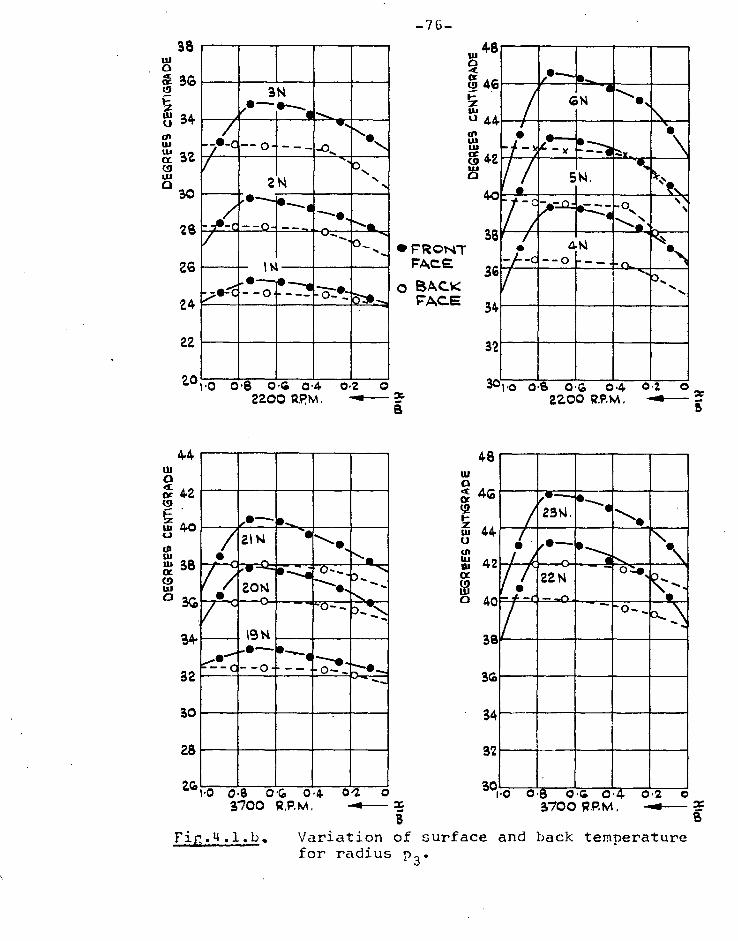
38 w 0 sfr 361

wu 34

to ICE' 32. w o 30

28

26

24

22

1.0 0.8 0 6 0.4 .2 o

/0 3N "h.-,

I *-----

/ • -,,,

•

2 N .. /-4,----4, 4

-.-C--O- - - -- -__ w....,

lk,, 0_ /

IN '-o_..,

....,,. 0 ----•

1.--111*--.

/ 614

e...... •.,s

\ • - -

• 41 -x--- 4:-.4. \

514. N •

/ 1

0

• 4W \

-...'s

w 48 0

w46 zu, U 44 U' us Eir9 42 c

40

38 • FRoNT

FACE 36 o BACK

FACE 34

32

2,0 .0 0.8 0.6 0.4 o 2 0

44 w a or 42

= w 40 co W• 38 OC

BG

34

32

30

28

4E

0 g 4

/". 2 w 4 us W 4 et

0 4

3

3

3

3

-76-

2200 RPM. B 22.00 R.P.M.

--A....".

A•

nd ob.,...._

w.,,,,

Iii-. w.,.. ....., 0.........

/6 /-0 t of

IP -0- --4- 20N

- --0‹

—c ( 7

0

1914

-0-

--"0-- c,....k..„.

w..........- - a-

el--1,-,-- .---- ___ - -

--e0-

,...... -0_

S

D • --......... 23N, 4/1\•

i• 2 •...........e......... 4\ /•/0--0

sdo • 22N . -

0- --(3--(' --o-,asq\ a

a

4

2

a 1.0 0. 0.6 O. 0.2 26.0 0.6 06 0.4 0.2 0 3700 R.P.M. 3700 RPM , x

Fig.4.1.b. Variation of surface and back temperature for radius p3.

-77-

pad. The pressure then drops'equally sharply (b) to below

the groove (ambient) pressure. A gradual rise and fall of

pressure occurs between (b) and the trailing edge, after

which the pressure rises sharply to the ambient groove

pressure (d).

A subsequent quantitative study of the leading edge

peaks (Chapter 6) showed that this sudden increase in pressure was partly due to a velocity ram effect at the leading edge.

The rotor surface emerging from the previous pad causes a

boundary layer formation within the groove, in which an in-

creasing quantity of oil is caused to travel with the rotor.

A proportion of this boundary layer is deflected by the lead-

ing edge of the next pad, causing an impulsive pressure

in this region.

A further contributory factor was the 45° chamfer

on the pad edge, which in spite of the very high angle of

convergence, can act as a normal tapered wedge.

Strong evidence was forthcoming of a second smaller

wedge in the leading section of the nominally parallel pad.

This "internal" wedge almost certainly results from local

thermal distortion as a result of comparatively large

temperature gradients at the leading edge, since the leading

edge is heated by dissipation heat from the body of the pad

and swept by colder oil in the groove.

Thus the three effects of velocity ram, 45° chamfer

and internal wedge contribute to a relatively high boundary

inlet pressure at the actual start of the parallel film.

These effects operate in the opposite sense at the trailing

edge. The true entry and exit boundary pressures are marked

on Fig. 4.2.

For an infinitely wide pad with an isoviscous and

-78- constant density film, the pressure would drop linearly be-

tween these two points, as shown. The effect of finite

width is to cause a non linear pressure drop due to the

effect of . ambient pressure at the sides of the pad.

The difference between this curve and the transducer output

was taken as the parallel surface pressure generation from

the density and viscosity wedge effects.

To determine the generated pressure it is necessary

to know both the entry and exit pressure of the

transducer concerned and the variation of boundary pressure

around the pad. From these boundary pressures the isoviscous

pressure field within the film can be found.

To find the boundary pressures it was necessary to

to consider in detail the flow and pressure conditions

in the groove.

b) Numerical analysis of experimental pressure curves

A typical transducer output across the groove is

shown in Fig. 4.3a. This was obtained by tracing a (x 10)

magnified image of the oscillograph film. The scale in the

x direction was found from the superimposed degree marker

output.

The crystal voltage output at any point can be

assumed to be the integral of the varying pressure over the

sensitive area of the crystal. Since the size of the

crystal is large compared to the size of the groove, there

will be an appreciable and variable difference between

true and apparent pressures from'point to point. This

difference was found to be particularly marked near the peak

of the curve. Since in some cases the inlet boundary pressure /was

-79-

effectively at this peak, it was necessary to find the

degree of attenuation by tracing out the curve of true

pressure. A numerical method was adopted as follows.

The crystal was divided across a diameter into

seven incremental areas of constant width (Fig. 4.3b). The

ratio of successive areas referred to the smallest area was

1.00, 1.66, 1.95, 2.05 (centre), 1.95, 1.66, 1.00. Twelve stations of the same incremental length were. marked off

in the x direction, starting from the groove centre (origin).

The signal height was measured in millimetres x 100 at each

station, relative to an arbitrary base line bb. These

values are recorded in row (d) of the calculation sheet

(Table 4.2). The true pressures p1, p2, p3 must at first be predicted, and the true pressures p_i, p_2, p_3 were

assumed symmetrical about the centre 0. The true

pressures in row (e) are multiplied by a waling factor to

give row (f) which is subsequently multiplied by 1.66, 1.95,

2.06, (the ratio of successive crystal areas) to give

rows g, h, i. Hence when the centre of the crystal was

at station 0, the crystal output would be proportional to

the summation of incremental pressure x incremental area

over the whole surface. This summation -3f, -2g, -lh, 0i,

lh, 2g, 3f (shown in the Table) sh6uld give the observed

value 2300. The actual ram 2357 is written in row (c)

and the residual +57 in row (b).

The centre of the crystal was then moved to station

(1), where all pressures were assumed known except'4(f),

which was found by making the summation equal to the observed

value. The true pressures 0 —,•-11 were thus found by

marchine through eight elements. The first run

gave approximate values only. A smooth curve, marked

TABLE (4.2). Numerical solution for a true pressure curve

a. Station -3 -2 -1 0 1 2 3 4 5 6 7 8 9 10 11 b. Residual OD OW +57 +1 -7 -14 164 -40 -57 -133 -325 c. Summation 2357 2631 3053 3716 4526 5260 5753 5867 5485

d. Observed - 2300 2630 3060 3730 4590 5300 5810 6000 5810 4590 32201500 e. Calc.(true)1790 2020 2200 2300 2400 2700 3300 3880 5350 7220 7400 6300 5100 3500 1500

f. .0886(1.00) 159.......179 195 204 212 239,0.292 344 474 639 655 558 452 310 133 g. 1.66 - 297 324 339 352 397 485 571 786 1061 1088 927 750 514 h. 1.95 - 380 398 414...°.466 570 671 925 1245 1776 1090 882 i. 2.05 ~418"435 490 598 706 974 1310 1342 1145

b. Residual +55 +8 +12 +26 -8 +48 +59 +2 -171 c. Summation 41/1 2355 2638 3072 3756 4582 5348 5859 6002 5639 MOD

d. Observed •110 2300 2630 3060 3730 4590 5300 5810 6000 5810 4590 3220 1500 e.(Calc.(true)17702000 2180 2320 2390 2710 3320 3930 5550 7320 7550 6550 5120 17861670

f. .0886(1.00) 157 177 193 206 212 240 294 348 481 649 669 580 454 335 148 g. 1.66 294 320 342 352 398 488 577 799 1078 1111 963 755 556 - h. 1.95 376 402 414 468 573 678 938 12 64 1303 1131 885 MEI

i. 2.05 422 435 492 604 714 987 1330 1370 1188

(A) Solution (2), (B) Solution (3).

-81-

j/////// /ii i

SECOM) SOLUTION

/ / /

ESsuRE rn.

‘4(/// / / / //

70

NO P2 m 90

50 FIRST SOLUTION

TRANSDUCER OUTOUT

b Ii 9 7 5 5

Fi7.4.3.a. Analysis of pressure transducer output

DIRECTION

MOTION

INCREMENT

LENGTH

. Crystal surface elemental areas.

-82-

"first solution" was drawn through these points and the smoothed

values examined for residuals, as shown in the top half of

the Table. The residuals were redistributed and a second

curve "Solution (2)" was drawn. This curve was also

examined for residuals and found to be within the accuracy

required.

This numerical method of smoothing by the use of

residuals was used in favour of an analytical method. Such

a method could involve the solution of seven simultaneous

equations for stations 3-9 in which the pressure at each

station was expressed in terms of the central pressure and the

three adjacent pressures on either side. This would

have involved the solution of eight (7 x 7) matrices for each

case, and the boundary pressures p1,2,3 and 1)10,11,12 would

have to be assumed and iterated until a smooth curve was

obtained. The described numerical method was found to be

quicker.

A total of ten entry and trailing pressure signals

were analysed for the test series and 2200 R.P.M. These

analyses showed some common results.

(a) The true pressure rise pt (Fig. 4.3a) from the central

groove pressures was.approximately 1.40 of the signal rise

Ps (b)The position in the x direction of max pressure was

very nearly coincident for the signal and the true pressure.

(c) Approximatdiy 50-60% of the pressure rise occurred in

the chamfer before the film was reached.

This analysis gave strong evidence for the existence

of thermally induced wedges at inlet and outlet. It was

-83-

PAD

TRUE PRESSURE CURVES,

OBSERVED PRESSURE.

0 oc w

WI

7

0

Fig. 4.4. Observed and true pressure curves for a cir-cular transducer with D/rc = 0.8.

-84-

thought possible that these wedges were caused by excess

cutting around the immediate perimeter of the pad during

the tapping process. Examination of the bearing under an

optical flat showed the interference lines to be quite

straight across the whole surface, indicating that these

inlet wedges were not a permanently machined feature. The

capacitance transducer signals were closely examined to deter-

mine the extent and magnitude of these inlet wedges.

Rapid analysis of inlet pressure

The numerical analysis was found too lengthy to

apply to every experimental case. A more rapid graphical

method was evolved. The true pressure rise in the chamfer

and internal wedge was assumed parabolic p = Pmax(1 x2/D2),

and an examination of a range of experimental results showed

that the pressure subsequent to the peak could also be

formalised into a number of different standard curves. These

standard curves subsequent to the peak are shown in Figure

4.4. The variables affecting the 44-,tenuation ratio

( max ',max indicated' true) are the relative transducer size . Dire and the form of curve after the peak. The outputs

of a circular transducer with D/rc = 0.8 are superimposed

on Figure 4.4. In this case the attenuation factor at pax is the same for curves 1, 2, 3 and larger for curves 4 and

5. Numerical solutions were obtained for values of D/rc = 0.6, 0.8, 1.0 and analytical solutions for values greater

than 1.2.

— _ ---. 4._ ...... ,

--.... ..,..0 -..&

..... 1,,,e- ...,

ss. .

cs, -..:.

N.,

1.o Attenuation Ratio

08

0.6

0.4

o2

I 8

Fir. 4.5. Variation D/r

/4 / 2 /o o e of attenuation ratio

06 P/r with c

-85-

The results are summarised in Figure 4.5, showing

the variation of attenuation factof, with Dire This ratio

D/rc was found for the four transducers in each test

(4 x 23), allowing the true peak inlet pressures to be.

calculated. Knowledge of this true maximum pressure

will enable correlation of theory and experiment for

the treble system of the velocity ram and the external and

internal wedges.

The pressure gradient in the approaches of the

trailing edge wedges are comparatively lower, and it may be

assumed that the transducer does show the true exit peak

pressure directly.

Analysis of wedge size

To attempt correlation of theoretical and

experimental pressures in the inlet region it is necessary

to know the amplitude and length of the internal wedge

which is apparent at the start of the parallel pad.

Direct measurement of this wedge size is

-86-

again affected by the relative sizes of wedge and trans-

ducer. A typical capacitance transudcer output across the

groove is shown in Figure 4.6a. For a truly parallel film the signal (curve (a)) remains flat until the edge of the

circular transudcer reaches the start of the 45° chamfer. This position was termed the cut-off point. 'Due to the presence of the wedge, the experimental curve (b) begins to

rise before the cut-off point is reached.

A similar 'marching' type numerical solution could

be used for this analysis, particularly since the six

starting values of capacitance are known at m = mo. Such

an analysis would give the shape of the wedge as well as

the amplitude. However it is known from classical theory that provided hl and ho are fixed, the pressure generation within the film is not greatly affected by the inter-connect-

ing profile (e.g. linear, parabolic, exponential). For these experimental cases, since the pressure rise in the

internal wedge was only approximately one third of the

total pressure rise, it was considered sufficiently accurate to obtain h

1 ocx/B° and h assuming an inter-connecting exponential

film h = ho e . The incremental capacitance was - postulated as m = mo —kx/B B. (Figure 4.6b).

Considering the circularity of the probe, the total capacitance can be expressed as

or

C = m A o o

x=B

+ f

x=0

x=B

2m1 .dx

C = m A o o e -Kx/13 2 2 (r Cr + x B) )2.dx

x=0

//

TRANSDUCER k- OUTPUT g- m

0 iL I

Ma

CID')

Fig.4.6a. Analysis of capacitance trace.

Fig.4.6b. Integration of capacitance.

- et x/8 ma moe

-88-

The variables involved are relative wedge size

p = B/r and the experimentally measured ratio mc /m o. The

amplitude of the wedge is governed by 0( since

h1/ho = -2" . The integral was evaluated either by

series expression or numerically for six values of p

between 0.06 and 0.96 for each value of p. The results

are shown graphically in Figure (4.7) which enables the value

of h1/ho to be found from the known parameters of p = B/r

and mc /m o. Both these can be obtained from the capacitance

transducer output curve, although the measurement of B is

approximate. For tests at high film thickness Amax nearly

coincides with the end of the wedge and B is better

measured from the experimental pressure trace.

The effect of capacitance side leakage.

The initial analysis showed the size of wedge

to decrease with decreasing film thickness. The'opposite

effect would be expected. The length of wedge B remained

approximately constant at 0.070 inches.

A large scale model of the transducer and the

opposing groove edge was set up as in Figure 4.8. The

probe, a 6" diameter disc, was separated from the simulated

pad by insulating blocks of negligible area. There was

found to be a difference in capacitance between the cut

off point and the centre of the pad when the same film

thickness was maintained in each case. The drop in

capacitance due to the presence of the chamfered groove

is shown below. (Over).

0

SID E

LEA

KA

GE

20

30

0

-89-

VALUtoc 0-5 o.6 0.5 0 4 0-B 0.2 0.1

0.20

040

0• BD_doll!'

A..0 ca--,.00

.„11111111111111edgerd

_

—

o W n —I 1.0 .:r ›'

—

I I I

V be°

1 I I I

COP V

I

0 0

i I I I

Fir. 4.7. Evaluation of wedge amplitude.

100

96

92

O

88 2 0

a 54.

80 2-4. 2.2 2.0 1.5

gm-no hi filo t•G

1.2 0

-Oa -04 .06 -08 RATIO kip .7. h + SET BACK

-15o Fir,. 4.10. Correction for side leakage.

FLUX LINES. BEARING

-90-

CA PAC ITANCE BRIDGE.

1 1 1 1 ////////////////////7/////7//7///////

Tip. 4.8. Model for evaluation of capacitance side leakage.

TRANSDUCER ROTOR

Fir. 4.9. Change in flux lines due to presence of chamfered edge.

-91-

h inches % Drop h/D

0.080 0.5 .013.

0.160 0.6 .027

0.220 0.9 .037

0.370 1.8 .062

These results are plotted in Figure 4.10 which

shows the correction which must be added to the

experimental ratio mc/mo before obtaining hl/ho.

The application of this method in practice showed

that in effect these wedges were too small to be measured

with this size of transducer, since the measured ratio

mc /mo was found to be of the order 0.98.

The analysis was only sufficiently accurate to show

that these wedges did exist, being approximately 0.070

inches long, with an amplitude ratio hl/ho increasing to

approximately 1.02 as the general film thickness was

decreased. A theoretical consideration gives the same order

of figures.

Due to this uncertainty in the magnitude of the

'internal' wedge, the correlation of theory and experiment

for pressure generation in the groove was restricted to

the contributions of the velocity ram and inlet chamfer

(Chapter 6).

4.3.The measurement of boundary inlet pressure

The pressure change through the leading edge region

can be considered as one of the family of curves in Figure 4.11. The pressure rises under the influence of the internal

wedge, reaching a peak at approximately the point where the

-92-

pad becomes parallel. Thereafter the pressure falls away

due to side leakage from the pad and the negative influence

of the viscosity wedge. This arrangement can be treated

analytically as a partially tapered film, with an

exponential shaped inlet of length B and a following parallel

portion of length A. The subsequent pressure drop in the region A can be treated by varying the lengths ratio A/B.

From solutions obtained with simple theory it was shown that the position of Amax remains very close to the end of the inlet wedge, except when A/B is very small.

The position of Amax for some values of A/B were:

A/B

2.0 0.05

1.0 0.07

0.5 0.12

0.0 0.39

Variation of h1/ho has little effect on the values of Ti/B.

These values are plotted in Figure 4.11. The analysis of

the experimental inlet pressure curves showed that Amax (true) and pmax (indicated) occur in very nearly the same

position. For tests at large film thicknesses, the

pressure gradient in the parallel section is low with

a/b = 2-6-3 = A/B. For these cases the length B can be

found directly from the experimental pressure outputs.

was found to be substantially constant with varying pad

temperature, although the wedge amplitude hi/ho would tend

to increase with temperature difference. The boundary

inlet pressure was found by marking offthe length b on

each transducer trace, as in Figures 4.12a, b.

The following values of B were measured for each

transducer path.

(a)

(b)

-93--

A Z B

=-13

II/111111/ I

r1g.4.11. Position of pmax relative to end of internal wedge.

Fir.4.12. Measurement from transducer outputs.

-94-

Transducer Wedge length ins.

p1 .065

P2 .088

P3 .087

P4 .071

4.4. Measurement of parallel surface pressure generation

The previous three sections have been devoted to

correlation and measurement of the factors which give a vary-

ing boundary pressure around the parallel pad. These boundary pressures have a direct effect on the pressure

within the pad boundary. Any deviation from this pressure

was taken as the effect of viscosity or density wedge.

Thus as a first requirement it is necessary to evaluate the

boundary pressure field, from which the transducer output

can be subtracted as shown in Figure 4.2.

Taking a simple form of Reynolds equation;

3 3

757' 2

rh • a x

+ 7E -12) (11 = 5U 75-7i - T

Assuming h and are constant

)213 0

)x2 )z2

The equation for pressure thus becomes Laplacian. The

solution of this type of equation is most conveniently

performed either by relaxation or by the use of a conductive

paper analogue. The latter method was selected due to the

large number of tests to be analysed. An analogue of the

same principle was used by Kingsbury (25 ) for the solution

of a tapered wedge with side leakage. In this case Kings-

-95-

bury used an electrolytic tailkt of varying depth to allow

for the variation of h.

The circuit used for the evaluation of the boundary

field is shown in Figure 4.13.

Fir. 4.13. Analogue for the solu-tion of boundary pressure field. A (x 10) plan of the pad was cut from

conductive paper (resistance 550 ohms per square). Voltages proportional to the boundary inlet pressures were fed into

the pad from terminals at each end of the transducer path.

The terminals were painted on with three coats of conductive

aluminium paint. The inner and outer radii were assumed to

be at constant pressures. The analogue was supplied from

a 5v. d.c. supply via a specially constructed potentiometer

from which the ten separate input voltages were taken.

The usual null-deflection method for plotting

equipotential lines was found most time consuming and a

high resistance voltmeter was used to find the drop in

potential along each transducer path.' This gave a voltage

error of less than i% from the null deflection method.

The entry and exit pressures for each transducer

were corrected for the radial pressure drop down the supply

groove. The pressures were converted into equivalent

voltages, which were set and checked before measurement.

-96-

The voltmeter was connected to each trailing terminal in

turn, and the voltage change measured down each transducer

path. This voltage curve was then reconverted to pressure

and the pressure decay curve between entry and exit was

plotted on each transducer output as in Figure 4.2.

The analysis of alternate tests at 1620 R.P.M. is shown in Figures 4.14a7 b. The boundary inlet pressure

becomes progressively lower than pmax. The transducer curve gradually departs from the boundary field pressure '

as the film thickness is decreased. This is to be expect-

ed from theory derived in Chapter 2 in which the viscosity

wedge pressure is shown proportional to Atb

Considering

the assumptions of constant film thickness of viscosity

pressure field Laplacian, the effect of dishing of the

bearing plate would be small at large film thicknesses.

The viscosity however will vary in the same magnitude for

all tests. This discrepancy should be shown in those tests

where the influence of viscosity wedge could be expected

to be small. However there is reasonable agreement of

transducer and boundary field pressure tests of large film

thickness (EG test 12N). This indicates the order of

accuracy in obtainin,g the parallel surface pressure

generation, although at large film thicknesses the method

does involve the subtraction of two equal order quantities.

The parallel surface pressure generation for the 23 tests

performed at four different speeds is shown in Figures

4.15 to 4.18.

It can be appreciated that this interference of

unequal boundary pressures is unavoidable in practice.

Nevertheless the author is unaware of any published work

in which these have been measured experimentally.

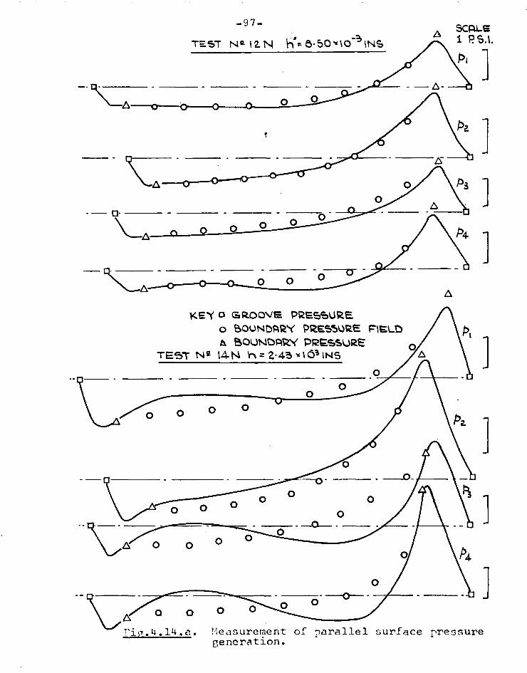
-97-

TEST N Q 12 N ha= 8-50'410-3 INS SCALE 1 P 5.1.

Pi

KEY D GROOVE PRESSURE o BOUNDARY PRESSURE FIELD A BOUNDARY PRESSURE

TEST N2 14-N h = 2 43 It 161 iNS

0 O

0 0 0

0

A 0 0 0

Neasurement of parallel surface pressure generation.

-98- ❑ GROOVE PRESSURE TEST 142 l6 N h = 2-4.3 X 163 INS 0 BOUNDARY PRESSURE FIELD

A BoUNDAW PRESSURE

4.14.b. Measurement of parallel surface pressure generation.

LESS 'NM...10.15

I.-. . (.0.007/1'....

/

•-.......... , ...., \

\ • \

N . \ \

2 ; .7, .

\ •...

% ‘ ` - ,

b ., doe

1-0

05

0

-0.5

-1.0

-99- 1-0

0.5

O

-1-0

710% .6-78

8N h = 3.76

5

0 77.... ... ..'.

/. %

'''. ...

. . A \

A • A . it„ .. . , \

` 4 .- ,

9N h=1-2.9

......

1

I' ''.....

,00 .•,4\

, f f

P., / \1/4

11 ....... IA

—.2„.".7-• /

A' r I A

1i..... 1

/ 1 I

I

I I,

I S I

I

,

a I ‘,......,

I

C iv .- N -.,--:- .4.

---11 ........ 4

I % I ‘../

I -% `.If %. . k x \

' \ / -

• % i.. .'"

\

t

1 \„... /

ION h= 1.0B

-10

10

5

0

-5

-10

- Is

-20

5

0

-5

-10

1 I N h.12, 0.78 Fig. 4.15. Parallel surface pressure generation 960 RPM.

•••• .0*

•••••... 1 .

14 N h=4.36

0 / •-...._ •

'%. .i.

\\

' •

• \

‘•

• ‘ 4

N ... .•

• •

..,v .,11

•••

.• ..' :

! s..,

4

2

0

-2

-A.

—(0 16 N hfr- 2.4S

-100-

-2 KEY 13N h=5-84 Pi

[12t.1 1,08.50 LE5STHANI Pa 0.2-6 PS).

" 4r. .... \y ...•

\ .,..

......

'ft....,

•

‘•••,......t

0

\ ‘• , %

\ • .

.• 0

ISN h= 2.93

2

0 O

1 .4 '• ,,„: ...... -"I , ........ di

2 P.SL •

4

2

0

-2

-4-

-6

la

8

4

0

—4

- 8

-12

• • •

....'•:-:\l' •

\ •

/ I/

\ NN.• •

..,.%, ."... ..a.... .4..

, t.•- - .....: , . . • , , , \. \ I:

. . \

.. . .... II /: .., , , ik. , ...-. ....,

la P5.1.

8

4

0

4

-8

-la

- 16 17 N N In:=1.0V

Fig. 4.16. Parallel surface pressure generation 1610 RPM.

—101- 4.

LE$S 141*-4 0.1 S

IN h= 9 54-

0

-2

-4.

4 P.S.1.

0

N 1-17-a..5S

..01.•••••••

. - •

5 tit ‘-‘t-- 4.75

,...- .- ... c.:".-'

..... ..7".N.N:N.N.cL0 1 ei

41v h=3.50

a

0

2

-4

4

2

0

-2

6

-6 -6

.. 4°- ""

SII

.

-.• % ..4% %,. %...

\\‘ /...."'-'"-.—"•.-1-...—........:zzsNs)

\0,

V •

N.

. -__ , i

. .

5 NI h= 2.G9

, - , t

\ \

i.,-- • \

k , N

N \N \ • ‘ •...„..,

N h=2,43

a

0

-a

6 RS.1.

4.

a

0

-2.

-4

Fig. 4.17. Parallel surface pressure generation 2180 RPM.

I•••• 4. ....

2,...c ••••••

Ss. N • oi#

.....„/

2

0

-102-

0

2

jY

19 N h 6•0(2,

...••••••

2.0 N

2

2

0

-2

2

0

-a NA 11=5.413

2 ZaN hz4.Q03

0

23 Ni 11=4.10 KEY

Fir. 4.18. Parallel surface pressure generation 3670 RPM.

-103-

4.5. Comment on results

A point of major significance is that the pressures

developed are predominantly negative. This corresponds

with the initial theory in Chapter 2 which predicts negative

pressures. It is in complete opposition to fact, in that parallel surface bearings are observed to run and support

useful loads. It would appear that the mechanisms of

density wedge and leading edge ram which have been given

to explain the operation of these bearings are overshadowed

by the viscosity wedge mechanism.

The characteristic shape of the pressure generation,

as shown by those tests at large and medium film thicknesses,

is shown below (Figure 4.19). Transducer p3 is selected.

Fig.4.19.Effect'of pad temperature profile. The pressure reaches a maximum negative point at

some one third of the pad length and then rises to give a

positive pressure in the trailing region. The initial

theory developed in Chapter 2 indicated a totally negative

pressure approximately parabolic in shape. The

difference may be explained qualitatively by consideration

of the true temperature variation along the pad. The

initial theory assumed a linear rise in temperature and

a consequent continuous drop of viscosity along the film.

In practice however the temperature was observed to rise

-104

to a maximum at x/B 2/3 and then to fall to a lower

temperature than inlet at the extreme trailing edge. This

could cause a reversal in the drop of viscosity, and hence

a positive pressure.

The'reason for this fall in pad temperature could be that both ends of the pad are swept by cold oil. This

would explain a drop of temperature towards the trailing

edge, but would fail to explain the significant fact that

the immediate trailing edge temperature is lower than the

leading edge, when the opposite effect would be expected.

An explanation for this fact is offered in Chapter

6 involving the diffusion of the hot layer of exit oil,

such that by the time the leading edge is reached,hotter

elements of oil have diffused vertically to sweep the leading edge, reducing the heat transfer and resulting in a

higher temperature than at the trailing edge, although both

temperatures ere considerably above that of the bulk of

the oil entering the groove.

Regardless- of the cause of this temperature drop,

the effect is to approximately halve the magnitude of

negative pressure. It may be remarked here that the

contribution of the density wedge is in opposition in both

positive and negative pressure regions to the viscosity wedge

mechanism.

The effect of three dimensions

The pressure generation previously considered has

been for transducer p3 near the centre of the pad. Pressures

at other radii show the same characteristic of passing from

approx. constan temp.

-105-

negative to positive, but do so at different points along

the pad. The test 16N is reproduced below to show this

effect.

RS). 2 rising

temp. \

i`

• ' \

0

-2 Fig. 4.20(b).

Effect of 3-dimensional pad

!Gm h-2-4-3 temperature.

This difference in transition may again be explained in terms

of the temperature change along the path of each transducer.

Examination of the pad temperature field shows that point

aT = 0 changes with radius as in Figure 4.20b. The point ax of zero pressure for each transducer corresponds approximately

to that point where .)x = 0.

Thus the pad temperature distribution has a primary

effect on the generation and distribution of pressure.

Two causes may be given for this shape of temperature

distribution. The change of temperature radially along the trailing edge is greater than that along the leading edge. The temperature rise along the leading edge is very

small. A particle of oil travelling through the film

will experience greater frictional generation at increasing

radii where both U and L are larger. This would cause the exit temperature to be higher towards the outer radius, and in turn tend to cause the observed temperature

distribution.

Secondly, the design of the bearing is such that

cooling is more effective on the inner radius than the outer

rig.4.20(A.

1 N. N

...N.6‘.,

\

N i \ .!

... -w •... i......,

(d)

rig.4.21.Effect of decreasing film thickness.

-106-

radius. The deep recess in the centre

of the bearing plate exposes a relative-

ly large area on the inner radius of

the pad to the incoming cool oil. This

oil will tend to be swept around the

inner side of the pad by the rotor

retaining nut acting as an impeller. The

outer radius is less effectively cooled

by a shallow groove in which the oil

will tend to be relatively stagnant.

This unequal cooling will tend to dis-

place the line of = 0 to that ob-

served, and hence affect the pressure

generated.

(a)

The effect of decreasing film thickness

The effect of decreasing film

thickness is to produce a definite

change of shape in the pressure generated,

although the pad temperature distribution

which induced the initial viscosity wedge

shape remained the same throughout,

altering only in magnitude. This change

is most effectively shown in the tests

at the slowest speed (Figure 4.15). At

slow speed the frictional generation is

lower and allows the pad closer to the

rotor before the 'limiting temperature

is reached.

The changes of pressure genera-

tion are shown schematically in Figure

4.21. The figure relates to transducer

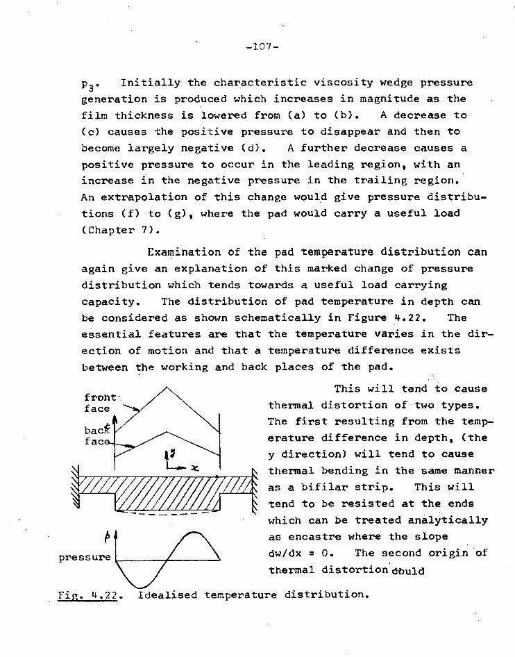
-107-

p3. Initially the characteristic viscosity wedge pressure

generation is produced which increases in magnitude as the

film thickness is lowered from (a) to (b). A decrease to

Cc) causes the positive pressure to disappear and then to

become largely negative (d). A further decrease causes a

positive pressure to occur in the leading region, with an

increase in the negative pressure in the trailing region.

An extrapolation of this change would give pressure distribu-

tions (f) to (g), where the pad would carry a useful load

(Chapter 7).

Examination of the pad temperature distribution can

again give an explanation of this marked change of pressure

distribution which tends towards a useful load carrying

capacity. The distribution of pad temperature in depth can

be considered as shown schematically in Figure 4.22. The

essential features are that the temperature varies in the dir-

ection of motion and that a temperature difference exists

between the working and back places of the pad.

This will tend to cause

thermal distortion of two types.

The first resulting from the temp- back fac= erature difference in depth, (the

y direction) will tend to cause

\ thermal bending in the same manner

4//7 A as a bifilar strip. This will

tend to be resisted at the ends 1

which can be treated analytically

as encastre where the slope

dw/dx = 0. The second origin of

thermal distortion dbuld

Fig. 4.22. Idealised temperature distribution.

pressure

-108-

be from the temperature change in the x direction. Considering

the expansion of metal in the x and y direction only, the

expansion in the direction y. will be greater than in the

central portion of the pad than at the edges. This direct

expansion in the y direction was termed fibre expansion, and

results in a distorted shape of the same form as the

temperature profile which induces it. The same expansion in

the y direction causes longitudinal strains which was termed

thermal bending distortion. Subsequent calculations (Section

7. 4) showed that both contributions to distortion were of

the same magnitude.

The shape of film resulting from such distortions is

shown in Figure 4.22. This is of converging-diverging shape,

which in the absence of the viscosity wedge would tend to

produce a positive-negative pressure generation. The fact

that the pad temperature profile remains substantially the same

shape throughout the tests, altering only in magnitude,

(Figure 4.1) indicates that this distortion is always present.

The distortion fails to take effect until the film thickness

is sufficiently low)when there is high frictional generation.

This would give increasing temperature differences and increas-

ing distortion. The geometric wedge action becomes more

powerful than the opposing viscosity wedge until a complete

reversal of pressure generation has taken place. An order of

magnitude analysis can show this effect qualitatively.

Assuming At c.4 1/h

I

2

hi 1 Pviscosity wedge tix h3

Now

-109- For small slopes,

1 oc T7-75 lope Pgeometric wedge

distortion c4 t 1 Now slope o< ho h0 2

Then pgeometric wedge o4

oc h

Thus the geometric wedge becomes increasingly dominant as the film thickness is decreased. This would

tend to explain the change in shape of the pressure genera-

tion as the fill thickness is progressively lowered (Figure

4.21).

Thus it would appear that "parallel" surface bearings

operate to produce a negative load when the pad is truly

parallel, but that the pad distorts to carry the useful load often observed in practice.

The dominant effect of temperature is evident in

all aspects of the parallel surface bearing, both in producing

the negative pressure when the pad is truly parallel and in

producing the distortion for the pad to support a positive

load.

In this range of experiments the process of change

from negative to positive load was taken as far as (e) in

Figure 4.21, corresponding to test 11N. Further experiments

with a modified bearing, allowing a greater degree of pad

distortion, demonstrated the whole change from negative load

to a useful positive load (Chapter 7). An analysis in-

cluding the wedge effect gives fair quantitative agreement

with results.

0

1

-110-

CHAPTER 5. Theory

5.1. Reeuirements and assumptions

The initial theory derived in Chapter 2, whilst use-

ful in indicating important parameters, requires some re-

finements to treat the experimental case. The temperature

rise along the pad is non linear and can be matched quite closely with the polynomial Tb = To + Atb (1.38x5/8 - 1.82x8).

The effect of frictional generation must be considered, part-

icularly since temperatures exert the primary influence on

pressure in the absence of a wedge. The assumption of an

adiabatic film gives an unrealistically high temperature rise,

sometimes of the order 200°C, and hence heat conduction into

the bearing solids must be considered. In addition the

effects of density wedge and tapered wedge should be incorporat-

ed as the bearing appears to operate on the tapered wedge when

taking a useful load.

To account for frictional generation the temperature

profile is assumed parabolic between Tb and Tr. The rotor

temperature Tr is again assumed constant. Figure 5.1 shows the

T/1Tb

, T

1,4 / /I x

1 <Jr Tr , /5-- ,.- r" .,-- ..-- ., ../

2S

Fig.5.1. Film tempetatures.

-111- postulated fill temperatures.

The solution for pressure follows closely on the

lines of the solution in Chapter 2. An expression is

obtained for temperature and hence viscosity at all parts of

the film. This expression is substituted into Reynolds

equation and a solution obtained for velocity u in terms

of dp/dx and other film variables. The solution of

velocity is integrated to obtain flow Q in terms of dp/dx.

The expression for dp/dx is integrated to obtain the local

pressure p. Detailed calculations are shown in Appendix 4.

During the solution for velocity u, it becomes

necessary to choose the power m in Slotte'srelation. This

power should preferably be a whole number since numerical

integration or complex analytical integration at this early

stage would make the eventual solution for pressure most

unwieldy. The power m is ideally 2.5 for the oil used, and

taking m = 2 gives a mean error of 2.5% in viscosity over

the range 200C - 500C in which most tests were run.

To incorporate the effect of density wedge, the

mass flow m = /)Q is taken as constant rather than the

volumetric flow Q. The mass flow can be expressed as

fiQ M flIFIra®

/7hU(1+M) =ARU(14-R)

when dp/dx = 0, (A4.4)

where 0 and M are large functions of temperature.

Film thickness variations c an be allowed for:

if expressed in terms of x. A suitable expression

is h = h1 (1 - d-f(x)), or h = h1 g(x). (A4.5). The integral

for pressure is;

[12 2 rUB 'ix' (1+M).dx1

h12 [g(x)j 2®

P =

x

K f dx' ..(A4.6) [g(x) p

-112-

All variables in the integral can eventually be expres-

sed in terms of LSt, x and the basic data to, tr, AtB. A

computer programme was written to perform the necessary inte-

gration and calculation of , the dimensionless pressure.

This programme, in Autocode suitable for the Eliot 803 com-

puter, is shown in Section A4.4.

5.2. Frictional generation

The film centre line temperature rise /St is required

for the evaluation of the integral variables. Detailed cal-

culations are shown iru section A4.2. The heat generated

is obtained in terms of a mean viscosity and equated to.the

heat conducted to the bearing solids plus the heat converted,

This heat balance yields a cubic equation for temperature rise

when Slotte's m = 2. To assist in the solution of this cubic

equation, the power m is temporarily taken as unity, giving

a quadratic equation in Zit for which an approximate solution

is easily obtained. This approximate solution is substituted

into the more accurate cubic equation and refined successively

by Newton's method of approximations. Five refinements

generaly gave convergence within eight significant figures.

Approximately half the computer programme is concerned

with the evaluation and refinement of At. This is used toget-

her with the basic data to, t r, B to evaluate 0 and 6 and hence M and ® . The integration is performed numerically

using Weddle's six strip formula for values of x' from

0(0.1) 1.0. Each integration for a certain value of x' required evaluation of the integral variables in steps of one

-113-

sixth between x' = 0 and x' = x', a total of 70 evaluations

for each case. The solution for Lit was given at each

value of x. Each case required approximately 21 minutes of

computer time.

5.3. Theoretical results

Figure 5.2 shows a typical set of computed values of

X • The contribution of density wedge increases with de-

creasing film thickness due to a greater film temperature

rise. The effect of increasing film temperature rise is to

increase the magnitude of positive pressure in the trailing

region. The generated pressure (p = 12 )2rUB/h2 x A ) can be summarised for all cases with a power law for p or max' p at x' = 0.3:

Speed R.P.M. 960 Amax = - 10.7h -2.03

1620 Amax = - 14.2h-1.74

2200 Amax = - 17.3h-1.625

3700 Amax = - 21.1h-1.65

where units of p and h are psi and ins x 10-3

respectively. In general the maximum pressure is some 40%

of that predicted by the initial: theory (Chapter 2) using

At3 as the linear pad temperature rise.

The pressure developed was found to be most sen-

sitive to the drop in temperature in the trailing region of

the pad. For the series fl tests this drop varied from 0 to

1.08 Llta below the leading edge temperature. An initial

value of r0..,133was obtained by averaging all 23 tests. Sub-

sequent examination of experimental pressures showed that only

the middle band of tests at each speed was useful for

correlation since measurement of experimental pressure was •

74---: T

i

(-o.4)

m— pi-- : \

l•/ 3,` i • 1

1 ,

•\

I I xis

1

_ .9 - •

. C. .5 .4 -2 .1

_/

/

_

3

/

Dimensionless pressure

0.61 A%151

10 PAD

0.5 TEMP:

0

-0.5

0.4

0

04

0$

1-2.

5

4

10

8

A tec 4-

2

0

//4/

.-------'-..--..."---s.-'.".. f

0

3 oc

1.0 8 .6 xf4- //3

o 1.0 •co4 2 . /13

0

TESTS- 1--Cos; 2,18o R.M. TESTS "7-TIN Zepikp.M. TENAQ..AT042.w RAE' PILIvl

Fig.5.2. Computer solutions for temperature and pressure.

-115-

difficult at high film thickness and distortion considerably altered the pressure at low film thickness. A figure of 0.44 temperature drop was found for those tests for which reasonable agreement could be expected.

In subsequent tests described in Chapter 7, the

temperature drop was taken as 1.38 for 960 R P M and 0.76

for other speeds. A special hypothetical case was evaluated

for temperature drops of 0.44, and 1.38, all other

data being constant. The results are given in Figure 5.3 and show the marked effect of this temperature drop on the

pressure developed.

O4, , ,

s 016

1.b8 I

Imo ta.

.1. ,... ... .. .. - ....._

o •

0a3

•

r. ab)484_

t..t.,.,„,"

WITH

1

-co,....,,c04 47=5.3

i

X x103 •E3

.4

0

0

.45 -3 x

-2 • 4 to =37•q t t. =43-4 0 Atz=2.4 1-1 al! 4

=1Gto -'8

PAD

0 TEMP.

to :-- 35.5 tr 3t3•0 Ate 2.7 h =OAS N =9`00

Fi2.5.3. Effect of trail-inn edge temperature drop.

Fig. 5.4. Effect of conduction to bearing solids.

-116-

The computed values for temperature rise are

shown below those for pressure. The effect of considering

conductivity to the bearing solids does not become pro-

nounced until low film thicknesses are reached. The input

parameter L = 8kB/pUh2C corresponds approximately to the

ratio of conducted/convected heat. The adiabatic isoviscous

temperature rise K, the actual temperature rise and the parameter L are tabulated below for some specimen tests.

Test 1N 6N 9N 10N 11N

K,(adiabatic) °C: 1.13 23.1 21.3 28.7 41.1

Actual rise oC: 1.60 7.28 4.32 4.40 4.40

.048 2.18 5.80 9.10 15.8

The effect of neglecting conductivity is shown in

Figure 5.4. The low value of film thickness makes this a

somewhat extreme case. Tests at higher film thicknesses

are not affected to such a degree. The curve marked

At = 5.3 shows dimensionless pressure considering conduc-

tion to both bearing solids. The remaining three curves

show the effect of allowing greater temperature rises along the centre line of the film until the full adiabatic case is reached. Consideration of conduction lowers the

effect of density wedge.

5.4. Treatment for side leakage

All solutions were for conditions measured along

transducer radius (3), and assumed an infinitely wide pad.

A three dimensional solution would require postulates of

the temperature field in three dimensions which in'turn

depends on external fractures affecting the three dimensional

heat transfer from the pad.

The distribution of temperature within the pad,

which na$ a direct effect on pressure, is discussed in

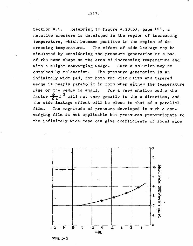
-117-

Section 4.5. Referring to Figure 4.20(b), page 105, a

negative pressure is developed in the region of increasing

temperature, which becomes positive in the region of de-

creasing temperature. The effect of side leakage may be

simulated by considering the pressure generation of a pad

of the same shape as the area of increasing temperature and

with a slight converging wedge. Such a solution may be

obtained by relaxation. The pressure generation in an

infinitely wide pad, for both the viscosity and tapered

wedge is nearly parabolic in form when either the temperature

rise or the wedge is small. For a very shallow wedge the

factor-Irz.h3 will not vary greatly in the x direction, and

the side leakage effect will be close to that of a parallel

film. The magnitude of pressure developed in such a con-

verging film is not applicable but pressures proportionate to

the infinitely wide case can give coefficients of.local side

."7

G 0

.s

4

.3 1

W 2 J

a 4 ji

O

1.0 .9 .8 .6 •5 4 .3 .2

F. 5-8

Shape & mesh size of anal-ysed area.

,.....„„,, "414VorftpW ‘144,

Ax 10

27 47) 48 Mil 49

Gil. 73 111

Pig65 54 141

1.07

pit. 1.06

.06 .1s 1,3

1.04

i4- p2 1.03

.(32 pi

1.01

1.00

1.02

-118-

1.00 1.01 1.02 1.03 1.04 1.03

1.00 1.01 1.02 1.03 1.04

1.00 1.01 1.02 1.03 Fig.5.6. Hypothetical

1.00 1.01 1.02 dimensionless film thickness. H

1.00 1.01

1.00

Fig.5.7. Dimensionless pressure.

I.06 1.07 1.08

1.06 i•OG

1.04 i.OS

1.03 1.04

i.02 1.03

1.01

1.00 4.01

1.00

-119-

leakage. These coefficients are applied to the infinitely

wide case of the parallel film solution.

Plotting of those points where the pressure changes

sign within the film yields a shape close to that shown in

Figure 5.5. The area is divided by an 8 x 8 mesh, giving

21 internal mesh points. One series of mesh points lies

directly on the radius p3. Figure 5.6 shows the hypothetical

film thickness values. The film thickness along p3 is set

to decrease linearly by 5%. To allow for dishing of

the whole bearing plate, the film thickness is set to increase

linearly with radius by 8%.

Relaxation solution

Setting Reynolds' equation into cylindrical co-

ordinates, assuming constant density and viscosity:-

6 r 3

a. 3 ap a h + -r-, - -57(h . ag ) = 611 -

Non-dimensionalising:

r = r'R, 8. = G'6, h = Hho

• A4 AR a2

A 4Jr a Froii3 + 1 rH3 bx r 49 ,

a ro d r r' 62 L Q

putting H3 = X, substituting finite difference formulae , and

rearranging yields the basic relaxation equation for each

point:

U = 27r RN.rt

p = 12 2 R2N /6h02

gives

-120-

A X1 1 o (rr'F) + A 2X2 + 1 A X33o CrirtF) + A X 3 4 4

- X (X11o rir'F + X2 + X3r3roF + X4) - 2 ,2 c

a )H

o d ro — = Residual o

-12 where F = [a6/b j , and a and b are dimensionless mesh

lengths.

Figure 5.7 shows the values of )1 obtained for

the relaxed net work. Those values in brackets are for an

initial coarse three point net work. Comparing the values of

pressure along p3 with an infinjtely wide solution of the

same wedge size gives the side leakage factors shown in

Figure 5.8. The factor drops by 50% over the length of the

pad.

The side leakage coefficient for the positive pres-sure area is larger and this results in a discontinuity of

the theoretical pressure curve for the whole length of pad.

Since the pressures are low in this region of discontinuity,

the actual discontinuity in the theoretical pressure is not so pronounced, and a fair curve can be drawn through all

points. This affect is shown in Figure 5.9, which shows

all theoretical points.

5.5. Aszreement of theory and experiment

Figures 5.9 to 5.12 show the agreement between

computed theory and experimentally measured pressures. As

suspected in Section 4.5, the basic shape of theoretical

pressure remains approximately the same through each range

of tests. The experimental pressures tend to a complete

reversal of this shape. The difference between theory and

experiment at low film thicknesses strongly suggests the

-121-

formation of a converging-diverging film.

For film thicknesses above 2 x 10-3 inches, the

film can be considered effectively parallel. Fair agree-

ment was obtained for those tests where the boundary field

pressure was not very close to the actual transducer output.

The following chapters deal with conditions in

the groove between pads and describe tests and results on

a bearing in which thermal distortion is greater than in

the tests already discussed.

3.76 0

-122-

Theory 8 N

0

[ * —,

"rhCON

.

.../.

.,..... ,--. .... ..,,E W•t% t .

's,

—

%

—

—

\

".... Ie

....-

0

/ \

/ .

/fr

/

/

•

.‘ ....0

4.0

PS.I

20

0

- 2

IIN.

to:0.78

0 THEORETICAL POINT.

0 THEORETICAL. POINT

IS

P5J. 75

0

-10

ao 0

hg1.29,

ION

h:1.03

P3.1.

0

- 20

Th.e..ons 0

0

0 THEORETICAL POINT

Fin.5.8. Correlation between theory and R

experiment 960 PM.

Ex.11.r.

Thew, y

P.S.I. 0

13 N.

hz 6.64

_ Exa. ...... -...,

...s.

- -- ..-

....-... /

2

14N,

hg4.361(103

---- ..... --,. -...„

Extl.C.

-

-.,

The.ork.6 --.. -...._ -

RS,I,

3

0

3

-6

161.4

Iv-Z.93063

_ The-0N -

•••••• - .../ /Exit,

-.., _ _

_ _

-----I ........ ....1

6

PS,1. 3

0

N -3 11:243 x10

-123-

Fig. 5.10. Correlation between theory and experiment 1610 RPM.

20

15

10 P.S.I.

5

0

-5

-10

-124-

_ Thcot

.,................/4 .-- -_

_ --.. ---

Ott. --.... .., ..., ...... --. -- --

17N

h&I•55%10

18N

K21.09)(10-3

30

25

20

15 P.S.1.

10

5

0

-5

-10

-IS

-20

-25

_ Theory

1-

)

_

_ --... ...-

rig. 5.10. Correlation between theory and experiment 1610 RPM.

Pm •

4 P.S.I.

a 0

-a 4

4N

11:3.50

-

_

...L... " '.... .-

-

-•.

•...,, ..., ...•"°'

P.S.1. 4

2

0

-2

-4

N

11:: 2.69

I0

0

-5

-I0

a 1

-125-

3N

4.78 0

P.S.1 GN

h: 2.13

Fig.5.11. Correlation between theory and experiment 2180 RPM.

.t

2-

2

tl.

-

PS,' 23 14.

hr. 4,10

-126-

4

2

0

22N

h=468

-2

-4

Fig. 5.12. Correlation between theory and experiment 3670 RPM.

-127-

CHAPTER 6. Mass and Heat Flow in the Bearing Groove

6.1. General

Two important practical effects are evident from

consideration of flow in the groove between pads. It can

be shown that a considerable proportion of the exit (convected) heat is carried to the next pad- This transfer of hot oil can lower the pad inlet viscosity by some large unknown factor

from the viscosity of the oil being pumped into the housing. This effect constitutes one of the major unknown factors in bearing design today, and applies to all types of oil fed

grooved hydrodynamic bearings.

A second effect of a groove is to impart a stagna-tion or ram pressure at the leading edge of the pad. Sub-

sequent calculations show that for the example of a 12 inch

mean diameter turbine thrust collar operating at synchronous

speed, a ram pressure of approximately 110 p.s.i. is produced

at the leading edge.

6.2. Boundary layer formation

Knowledge of the velocity field in the groove is

necessary for the solution of both the hot oil carry over

and velocity ram effects. As a first criterion it is nec-essary to establish whether the flow is laminar or turbulent.

The outflow of oil from the back of a pad could be considered

analogous to a liquid-into-liquid jet, with the rotor surface being the centre line of the jet of velocity U. Andrade

( 26) has reported that for such a jet, flow is laminar for

efflux Reynolds numbers of up to 30. The majority of oil

bearings operate below this figure. It is also likely that

the flow remains laminar throughout the groove.' The critical

length Reynolds No, Rex for transition from laminar to tur-

bulent flow on a flat plate is usually taken as 10g. Using

-128-

the groove width as the dimension, this value is rarely ex-ceeded in practice. Hence in the analysis, the flow is assumed laminar throughout the groove.

Oil enters the groove (Figure 6.1) with a velocity profile primarily governed by the wedge ratio hi/ho.

Re-roiz.

F7I61.

At some point distant from the pad exit, the standard boundary layer profile will be adopted. If this distance of change to the standard profile can be shown to be very small, then the usual.steady state boundary layer techniques can be used to find the whole velocity field. With this object in view, the propagation of a typical exit protile was found using a finite difference method developed by

Witting (27 ).

Witting's method for propagation of a boundary layer profile

The following assumptions are adopted:

1. The flow is laminar and incompressible.

2. The problem is two dimensional. 3. Viscous forces are negligible.

These assumptions_ lead to the boundary layer equations:

-129-

u 4. v = _ 9 e) 2u 6x ay /0 dx a y2

.?4u , v 0. -57c ay - (dp/dx) is taken as zero in the groove. Expressing the para-meters in non dimensional form:

x* = x/ho y* = y /Re/h, u* = u/U, v' = v die/U

where Re includes the dimension ho, and using the continuity

equation to eliminate v:

u--- au au u 12_ a x by w;.dy = (in dimensionless form)

o eu eu rY 2u a 2u 2 ;14—FT,F).dy u and hence a y2

The right hand side of this equation contains only

derivatives and integrals with respect to y and can be evaluated for a known initial profile. However the evaluation Of au/ ax requires particular care due to certain singular-

ities exhibited by the boundary layer near the wall. At the wall the velocity is zero in both directions due to the

no slip condition and both terms of the equation assume the undeterminate form 0/0. Furthermore, at the wall the inertia terms are zero and hence ( a 2u/ ay2) = 0. Witting

assumes a polynomial for the velocity profile and develops an iterative method for the solution of the propagated profile.

Example

Take U = 1000 in/sec. ins.

= = 2 x 10-3 = 6.65 x 10-6 Reyns.

= 0.032 lb/in3 .

whence Re = 25.

o•c. 0 0./ o 2 0.3 0,4 0,5 biMENSioNLESS VCLocrne

Fig. 6.2. Propagation of an exit profile'by Witting's method.

N G'S I' succ S _wces Divrtk PAD FROM

c% rr %), 'NAP 11.6 11 EsArr 0% % :02

3 to 4 ' Oq S ' G

gla .7 t4 8 ' CI .3° .36 10

.....,_ ........ .........

sultry::: IC C c . , .."-"•,„

Z.% 1 ).• • . . 4 4. ...;,...... PRop 3 ‘°

... ...% %,„%,‘ ,, 4...

4 , 1Z

10

.4%...„.........

4\ .!'` \

• $ ‘

4. %\

12

I0

Co

0

PAD

/ / //

/.0 o.q

FIL

M T

HIC

KN

ESS

-131-

An outlet profile of u* = (y/h)1/3 was assumed. This is arbitrary but corresponds to a relatively large value of hi/ho. Figure 6.2 shows the successive profiles obtained using the finite difference method. The choice of

mesh size was governed by the accuracy required. As the curvature of the profile decreased, larger mesh lengths could be used. The following values of mesh length were used for

the ten propagations:

uo - u3 0.01 (x/h) u3 - u6 0.03 (x/h)

u6 u10 0.06 (x/h)

TOTAL 0.36 (x/h)

Figure (2.6) shows that the final profile, which is almost linear, is reached after the very short distance 0.36 (x/h). This indicates that the standard boundary layer pro-file is formed very close to the pad exit. Since the groove

length is normally at least 100 x h$ the effect of the

particular shape of the exit profile can be neglected.

6.3. Thermal effects in boundary layer

The boundary layer will grow in thickness along the

groove as more static fluid is entrained by the moving

rotor. The layer of hot exit oil will also expand into the boundary layer, but at a slower rate.

TOKUNCIPS vitocMV

PAT) . /....._ —

h r!

1___•_ x 120 -rack

•

/ / /1/ 1111.

14411114AAL To voi OiliS

U

Fig. 6.3. Formation of thermal boundary layer.

•1

-132-

It is shown in standard boundary layer theory, that

the growth of boundary layer thickness over a flat plate is

given by bb 5.0(X/Re)2 where S* = i/h, X = x/h and Re contains h. The value of the coefficient is dependent on the particular polynomial derived for the velocity profile.

The origin of X can be taken as the pad exit. For flow over a hot plate it can be shown that the ratio of velocity and

thermal thickness is given by cr = g/crt = 1/Pr1/3, where

Pr is the Prandtl number c/g/k. The Prandtl number for the

oil used is of the order 3000, and hence cr is generally less

than 0.10. Since at the origin 6.* = dr* = 1, the thermal thickness in the groove may be approximated by:

at = 6 — 1)132,-1/3 + 1.

6.4. Varying viscosity boundary layer

If the rotor surface is assumed to be at constant temperature, there will be a large variation of viscosity through the thermal layer from r to the viscosity of the sup-ply oil 7 s (Figure 6.3).

Since the velocity gradient is maximum in the sur-face region, it might be expected that the velocity profile would be influenced by this varying viscosity which can change by a factor of six through the thermal layer.

A full derivation of the varying viscosity boundary layer is given in Appendix A5.1. The viscosity varies

through the thermal layer in some unknown way which will be partially dependent on the degree of frictional heating in the pad. Two different expressions for viscosity were

assumed, (Figure 6.4.), and the condition a/ a y( rt•au/ ay) = 0

1."6. 2. 3 4-

Flei.G4 Assumed variation of viscosity through thermal layer.

tzu

-133-

i I SOVISC-OLIS

0 MERMAL

L.04%tate. O

RoTDR Su FZFAP-M,

tb

1

I

\ VISC.cetry

114 FLoV4c6C, \

fi 1 \ ' s 0./ Iscpcs

Via?

0 2 4 .C. t-C)

Comparisow,of isoviscous and non-isoviscous velocity profiles.

16

8

4

applied in the thin thermal layer.

It was assumed that this condition, which implies

negligible inertia forces, could be applied in a thin region close to the wall. The corresponding condition for the iso-viscous boundary layer derivation is ( e2u/y2)o O. The solution for velocity in this region was -matched with a polynomial expression for velocity above the thermal layer.

Figure 6.6 shows the derived velocity profiles for = .091 and viscosity ratios of N s 2, 4, 6. For each

ratio; the profile was evaluated for the two different viscosity profiles shown in Figure 6.4. Figure 6.6. shows that the boundary layer thickness increases with increasing N, but that the whole velocity profile is not greatly affected by the choice of viscosity profile,- particularly at lower values of N. It is interesting to note that within the thermal layer, the velocity is not greatly affected by either N or the manner inwhich viscosity varies. This fact could be

extremely useful when considering the thermal transport effects

14h

ah

of toh

pi 0 1- 0 of

6h L

111 4h

4

h

-134-

I

KEY PROFiLE 0 .1)

N = a 0 • 1.4 7_ 4. 0 n 1.4 . co A A

n I • 0

. A

1 !t

•

El

8% el \

\

.

itk •

. 0 A ,ea

... is a .... NA. A Ntx . ..

. .

. • A 0 A a .

0 0.2. 0.4 0.6 0.8 10

INFig. 6.6. Effec trof viscosity profile and viscosi ratio on boundary layer.

-135-

in the analysis of hot oil carryover, since interation between the temperature, (viscosity) and velocity fields would not be necessary.

The derivation of the velocity ram pressure at the extreme leading edge of the pad is described in full in Appendix A5.3. The additional pressure rise from the 450 chamfer is included. A tentative correlation of theoretical pressure rise with experimental results is given in Tables 6.1 and 6.2. The experimental values were obtained directly from the transducer outputs at the start of the nominal parallel film. The correlation cannot take into account the effect of the small thermally induced wedge in the leading edge region described in Section 4.2, since the capacitance transducer was too large to measure this accurately. Such a wedge would tend to increase the ram pressure and hence the theoretical values, which take no account of this wedge, should be slightly lower than the experimental figure.

Tests were carried out with two different groove

widths. The first (N) test series was with an effective groove width of 0.145 inches. For the second (P) series, three

of the six pads were removed, giving an effective width of 1.580 inches between pads.

The agreement for tests with a small groove (0.145 ins

could be affected by the following factors:

a) The negative pressure influence exerted by the viscosity m! wedge in the main portion of the pad.

b) The higher pressure gradient in this series would lower velocities in the boundary layer, thus affecting the ram

pressure.

c) The parabolic temperature exit profile would not be ,

greatly attenuated over this sort distance, giving lower

-136-

Leading edge pressures for radius p2

First bearing: Groove width 0.145 ins.

Theoretical Pressures Test Film Viscosity Velocity Viscous Total Expt.

Thickness Ratio Ram Ram Theory Pressure ins x 10-3 psi psi psi psi

960 RPM. Stagnation Pressure = 1.01 psi

N7 6.78 1.43 0.48 1.16 1.64 0.86 N8 3.76 1.75 0.49 2.15 2.64 1.91 N9 1.29 2.86 0.51 4.80 5.31 2.29 N10 1.03 3.26 0.51 5.35 5.86 2.41 N11 0.78 3.77 0.51 5.97 6.48 5.30

1610 RPM. Stagnation pressure = 2.81 psi

N'12 8.50 1.71 1.18 1.05 2.23 1.43 N13 5.84 2.18 1.24 1.46 2.70 N14 4.38 2.48 1.27 1.90 3.17 2.40 N15 2.93 2.87 1.30 2.71 4.01 2.92 N16 2.43 3.01 1.11 3.10 4.41 2.58 N17 1.55 3.72 1.33 4.22 5.55 3.12 N18 1.09 4.64 1.33 4.99 6.32 4.43

-2180 RPM. Stagnation pressure = 5.15 psi

N1 9.34 2.25 1.98 0.99 2.97 1.22 N2 6.55 2.71 2.13 1.43 3.56 1.95 N3 4.78 3.18 2.20 1.86 4.06 N4 3.50 3.74 2.26 2.38 4.64 2.96 N5 2.69 4.12 2.30 2.87 5.17 2.81 N6 2.13 4.55 2.32 3.43 5.75 2.83


NIS 8.06 2.43 4.65 1.21 5.86 2.03 N20 6.37 2.96 5.01 1.41 6.42 2.96 N21 5.48 3.22 5.19 1.58 6.77 2.62 N22 4.68 3.48 5.38 1.83 7.21 3.86 N23 4.10 3.72 5.50 2.17 7.67 4.27

TABLE 6.1

-137-

Second Bearing. Groove width 1.58. ins. Theoretical Pressures

TEST Film Viscosity Velocity Viscous Thickness Ratio Ram Ram ins x 10-3 N psi psi


Total Theory psi

Expt. Pressure psi

2P 3.31 1.29 0.43 2.40 2.83 3.30 3P 2.67 1.39 0.43 2.91 3.34 3.48 4P 1.62 1.54 0.44 4.78 5.22 4.52 SP 0.99 1.78 0.44 7.34 7.78 6.00 6P 0.77 1.93 0.44 8.86 9.30 9.80 1610 RPM. Stagnation pressure = 2.81 psi 11P 9.40 1.25 1.15 0.95 2.10 2.92 12P 6.08 1.53 1.17 1.50 2.67 3.54 13P 3.65 1.71 1.19 2.67 3.86 4.81 14P 2.45 1.80 1.20 4.06 5.26 5.24 15P 1.90 2.09 1.20 4.98 6.18 5.39 16P 1.60 2.22 1.21 5.62 6.83 6.93 17P 1.19 2.47 1.21 6.95 8.16 10.35 2180 RPM. Stagnation pressure = 5.15 psi 20P 5.64 1.56 2.11 2.13 4.24 3.48 21P 4.29 1.76 2.13 3.01 5.14 5.76 22P 3.38 2.03 2.15 3.26 5.41 6.95 23P 2.40 2.37 2.16 4.15 6.31 7.10 24P 1.50 2.65 2.18 6.40 8.58. 9.40 25P 1.27 2.76 2.18 7.28 9.46 13.6 3670 RPM. Stagnation pressure = 14.5 psi 28P d.85 2.27 5.59 1.52 7.11 9.4 29P 4,83 2.52 5.74 2.25 7.99 10.7 30P 3.53 2.76 5.83 3.12 8.95 12.1 31P 2.86 2.86 5.86 3.86 9.72 12.2

TABLE 6.2

-138-

viscosities in the thermal layer than expected. This would

also tend to reduce velocities.

In the second series of tests with a much larger

groove (1.580 ins.), factors (b) and (c) would not be so

effective. The negative pressure influence of the

viscosity wedge is shown in those tests at large film thick-

ness. At tests of medium film thickness were pad distortion

counteracts the viscosity wedge, agreement is good.

It can be seen that changing film thickness has

little effect on the velocity ram pressure, which for design

purposes could be taken as 0.4 x stagnation pressure or

peel ram 0.4/2U2/2g.

The generation of ptessure at the leading edge is particularly important with parallel surface bearings, since

this is effectively the only source of positive pressure when

the film is actually parallel. The leading edge chamfer

is beneficial to lift and could be the main source of load

carrying capacity before distortion takes place to carry the load. A shallow chamfer on the leading 20% of the pad would

assist load carrying during the heating process. Such a

chamfer could be made by hand scraping or by cold forming on

such items as crankshaft thrust washers.

6.6. Hot oil carry over

The complete solution of heat and mass transfer in

the groove is clearly a most complex problem. For a full

solution, a complete thermohydrodynamic analysis of both the

pad and groove together is required, since both systems inter-act. The full details of an approximate analysis is given

in Appendix 5.5. This gives fair agreement with experimental

results.

-139-

The primary assumptions are that the rotor remains at constant temperature and that the temperature profile

at any point can be represented by a simple power law. Fric-

tional heating above the rotor temperature is neglected,'

and the exit oil is assumed to be all at the rotor temperature.

Conduction from the rotor is allowed for.

The predicted values of pad inlet temperature for

alternate tests are given in Tables 6.3 and 6.4. Thermal

boundary layer theory indicates that the temperature profile is nearly linear close to the rotor surface, and hence experi-

mental values are taken as the mean of the pad leading edge and

rotor temperatures i.e. i(to + tr).

The analysis gives the proportion of heat carried

over in the form tm/41t„ where 41t = tr is and tm = pad

mean inlet temperature. For an infinitely small groove, the

factor tm/At would be unity. The theoretical and experimental percentages of heat carried over are plotted in Figures 6.7 and 6.8. These figures show the effect of

speed and film thickness on the degree of hot oil carry

over.

6.7. Comment on results of heat carried over

A most interesting geiteill result is that the quantity of heat carried over is high, between 70% and 95%. Further-

more, this quantity is not greatly effected by speed, film

thickness or groove width. The effect of neglecting any frictional generation within the pad that is higher than the rotor temperature becomes less pronounced with the larger groove, where better agreement is obtained.

Such excess frictional generation would give an approximately parabolic temperature profile, such as con-sidered in Chapter 5, and is largely responsible for the dis-crepancies with the smaller groove.

•

-14C)-

Results: Hot oil carry over

and tm/dt 2 S*

E.-(1-1/2611)al

From solution f:

lT 0.5 + t

0.145

X a f(as cf) = -

Groove length:

Pr.Re

ins.

= a+1

Speed Test Film 3. tm/At Predic/ed Experimental RPM No h x 10 inlet C Inlet 0C ins 960 N7 6.78 .698 24.2 24.8

N9 1.29 .695 32.8 37.0 N11 0.78 .740 39.0 44.2

1610 N12 8.50 .723 '28.6 27.9 N14 4.38 .691 33.4 34.7 N16 2.43 .673 36.6 40.7 N18 1.09 .688 45.2 51.3

2180 N1 9.34 .750 30.7 29.1 N2 6.55 .733 33.0 32.7 N4 3.50 .691 37.6 40.8 N6 2.13 .660 41.0 46.4

3670 N19 8.06 .754 41.3 38.9 N21 5.48 .715 45.5 45.0 N23 4.10 .705 47.7 48.8

Table 6.3. Correlation of predicted and experimental

inlet temperatures. Groove length = 0.145 ins.

Results: Hot oil carry over

tm/41t Predicted inlet °C

Experimental inlet °C

Groove length: 1.580 ins. Speed RPM

Test NO

Film 3. h x 10- ins 960 1P 5.12 .701 28.4 28.8

3P 2.67 .732 30.0 30.7 SP 0.99 .852 34.3 35.0 7P 0.75 .870 37.1 38.1 9P 0.72 .883 40.5 41.4

1610 12P 6.08 .683 31.0 31.4 14P 2.45 .725 34.0 34.9 16P 1.60 .761 37.1 38.8 18P 0.89 .833 41.4 43.0

2180 20P 5.64 .618 31.9 33.0 22P 3.38 .692 35.4 36.7 24P 1.50 .755 41.5 43.5 26P 0.91 .813 45.7 47.1

3670 28P 6.85 .691 41.0 40.4 30P 3.53 .681 43.9 45.2

Table 6.4. Correlation of predicted and experimental inlet temperatures.

Groove length 1.580 ins.

100

90

- 80

of • 70

of

O Go >- 01

so

• 40

30

A • kg:,

3s

-..

6,0*

0-., ••••.. ..... Twit a...

et o 36

13 4153. 044--

0%0

-- =To eGo ,......b, _-.... !Gip

.

Er asP• :=7-0.... Zr.----*

GROOVE VV1OT14

SPEED TNE012.s< . 960 0

MAO A

2160 0

3670 V

0.1451tos

EXPT. • • a • ,

N.)

CPS 077 1,5 2.0 4 M 71-41CKNS it4c3)6,10-3 Fin. 6.7. Effect of speec ana tiim thickness on hot oil carry over,

groove width: 0.145 inches. zr

4.• •

100

90 2

Di so a. 1

1.0 7o 0

oi

4 GO

JU

50 0

40

30

e),„ `-• 960

`'..... '"'.0 '4"4` .....,

•

*"....N%

0 ‘6....i.ko

E.

.., %Ge. -.RI ‘<- ...„,. .....,...

'''''.... I .... q0

p .., ........ ......

•••• o 46..""" -..... .......

..... --...--- -... s--.. -..,

--... '..."

,,......... - --...

— biro6321r

--.• =

.-7

A IZOON E \N 1 DM

Spew) -r-44EDR4 - 960 0

1610 A

al SO 0 3670 V

, .

1 , 660 DNS

GI( PT • • • V

. 5 077 f 1.5 a 3 4 6

8 FILM TI-IICKMESt, INS .4 IC53

Fig. 6.8. Effect of speed ondfilm thickness on hot oil carry over, groove width 1.58 inaes.

-144-

Increasing speed lowers the hot oil carry over slightly, but decreasing film thickness results in more heat being transported. The most striking result is that the attempt to decrease the hot oil carry over by greatly in-

creasing the groove width is quite ineffective. This. result gives justification for the assumption used in the

analysis of both pad and groove that the rotor surface tempera-

ture remains approximately constant. The poor degree of heat

dissipation in the groove is largely inherent from this fact, together with the high Prandtl number of lubricating oils.

Hot oil carry over

the experimental measurement

leading edgVitil the trailing

The leading edge is swept by

thermal layer. This effect

pressure in the rear portion

offers an explanation for

of a higher temperature at the

edge of a pad (Section 4.5).

hot oil deflected upwards from the aids the generation of positive

of the parallel pad.

The degree of hot oil carry over may be found using

this analysis, although the value of rotor temperature for any

given set of conditions remains unknown. Such an analysis

would be governed by basic design of the complete bearing

arrangement.

The rotor runs at a higher temperature than the pads,

and cooling of the rotor is likely to be more effective in

improving bearing performance than cooling the pads. This

would directly increase the pad inlet viscosity and hence the

load carrying capacity. A simple method of rotor cooling

for rotors which run fully immersed in lubricant is shown in

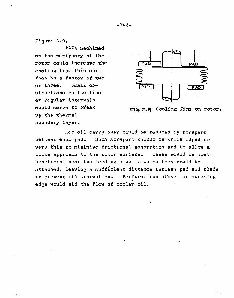
-145-

Figure 6.9.

Fins machined

on the periphery of the

rotor could increase the

cooling from this sur-

face by a factor of two

or three. Small ob-

structions on the fins

at regular intervals

would serve.to bx(eak

up the thermal

boundary layer.

Pet- G* Cooling fins on rotor.

Hot oil carry over could be reduced by scrapers

between each pad. Such scrapers should be knife edged or

very thin to minimise frictional generation and to allow a

close approach to the rotor surface. These would be most

beneficial near the leading edge to which they could be

attached, leaving a sufficient distance between pad and blade

to prevent oil starvation. Perforations above the scraping

edge would aid the flow of cooler oil.

-146-

CHAPTER 7. Second Test Series

7.1. Procedure

The bearing used in the N test series was modified by removing alternate pads. Photographs of this modified bear-

ing are shown in Figures 7.1 and 7.2. The object of the

modification was to increase the temperature differences and

hence distortion within the bearing, and to find the change in

hot oil carry over for a much larger groove.

The experimental procedure of testing and recording

was as described in Section 3.8. Tests were run at four

different speeds.

7.2. Results

The results are given as follows:

Tables 7.1 and 7.2 give general test data, some specific pad

temperatures, rotor' surface temperatures and estimated distortion

The pad surface temperatures were of the same general

form between to and Atb except that slightly different ex-

pressions were used to describe the shape. Figures 7.3 and

7.4 show the two dimensional temperature field on radius (3)

for some sample tests. Figures 7.5 to 7.8 inclusive give the

pressure transducer outputs for each test. Since a useful load

could be. carried (subject to certain conditions), the actual

pressure generated by all mechanisms was thought to be of more

interest than treatment of these pressures to subtract the

boundary effects. However a sample of the generated pressures

and boundary field subtracted is shown in Figure 7.9 for

1610 RPM. Further results or treatment of results are given

during the discussion.

CALCULATION SHEET P SERIES TEST RESULTS NOMINAL SPEED 960 RPM

TABLE 7.1

TEST Ins Speed Ambient Torque Oil Nous- to 4tb t1 t2 t3 t 4 Distortion NO x10-3 RPM press. in.lb. Flow ing ins x 10-6

kt psi gpm inlet

temp°C 1P 5.12 962 29.2 11.7 1.33 25.9 28.1 0.7 28.9 29.4 29.8 29.4 8.0. 8.9 2P 3.32 962 36.5 14.1 1.22 25.9 28.9 1.7 29.9 30.1 30.9 30,1 14.4 14.5 3P 2.68 962 37.3 15.5 1.16 25.8 29.8 2.1 30.8 31.5 32.1 31.9 18.0 17.8 4P 1.64 962 38.7 19.3 1.12 25.9 32.2 2.6 32.5 33.3 34.5 33.8 23.5 23.7 5P 1.02 962 34.4 23.2 1.13 25.6 34.2 2.7 34.4 35.8 36.4 36.6 27.0 27.3 6P 0.78 962 34.1 25.8 1.14 25.9 35.5 2.7 36.7 37.6 38.0 38.4 27.9 29.8 7P 0.77 962 33.5 28.2 1.13 25.8 37.4 2.0 37.9 38.8 39.5 39.8 27.8 31.9 8P 0.76 962 33.2 30.8 1.13 25.8 38.3 2.3 39.5 40.6 41.2 41.4 29.0 32.4 9P 0.75 962 32.7 31.2 1.13 25.8 40.4 1.8 41.4 42.4 42.8 43.1 31.3 37.5

NOMINAL SPEED 1620 RPM 11P 9.40 1620 14.4 12.6 1.41 25.4 27.6 1.3 28.2 29.2 30.1 29.6 11.1 10.7 12P 6.11 1620 26.2 13.4 1.38 26.1 29.5 1.6 32.2 33.3 33.9 32.6 15.4 15.9 13P 3.65 1620 37.5 18.7 1.23 26.2 31.. 7 2.7 34.3 35.6 36.7 35.9 23.8 24.6 14P 2.48 1620 42.4 22.1 1.17 26.5 32.9 3.7 35.2 36.9 38.0 37.2 30.4 30.6 15P 1.92 1620 42.9 23.4 1.12 25.9 34.6 4.6 37.7 39.2 39.8 39.6 37.2 36.8 16P 1.62 1610 44.4 24.8 1.11 26.1 37.0 5.4 38.8 40.6 41.5 41.4 44.3 44.2

617P 1.21 1610 44.9 26.9 1.10 26.4 39. 45.6 41.3 43.3 44.4 440 49.3 5.00 18P 0.91 1610 44.2 29.1 1.11 26.7 41.6 5.2 42.2 44.4 44.9 45.2 50.5 5.29 19P 0.78 1600 43.2 32.8 1.13 27.0 43.4 5.0 45.8 47.6 48.5 486 53.1 57.3

CALCULATION SHEET P SERIES TEST RESULTS TABLE 7.2


TEST Speed Ambient Torque Oil Hous- tl t t3 t4 Distortion NO. insx10

-3 RPM pressFe in,lb. Flow ing 2 ins x 10-6

lb/in gpm inlet temp 0C

20P 5.64 2200 27.4 18.8 1.40 26.8 31.6 2.2 32.7 34.3 35.2 35.0 22.9 23.9

21P 4.29 2190 31.5 19.6 1.23 25.1 32.0 3.0 34.6 36.0 37.3 36.9 29.1 30.6

22P 3,39. 2190 35.6 20.2 1.25 26.5 34.0 3,3 37.6 39.3 40.6 40.1 30.0 31.4

23P 2.40 2185 39.7 22.2 1.20 27.0 37.4 5.2 41.1 43.1 44.1 43,6 45.346.1

24P 1.52 2170 41.2 23.8 1.19 27.2 40.8 7.0 44.2 46.1 47.4 47.4 59.5E0. 1

25P 1.29 2170 41.4 25.8 1.19 27.5 43.2 7.3 45.6 47.2 48.3 48.9 66.868 .8

28P. 0.93 2170 41.3 27.4 1.18 27.0 44.3 8.1 48.1 49.8 50.6 51.4 70.5 71.6

27P 0.85 2170 41.2 28.4 1.19 27.9 45.8 7.8 48.5 50.2 51.4 51.9 72.2 74.1


28P 6.85 3680 17.0 19.0 1.44 29.8 34.8 2.7 44.0 46.0 47.7 47.7 23.5 24.3

29P 4.83 3610 25.6 20.7 1.40 30.0 37.4 3.6 46.1 48.5 50.1 50.6 35.3 37.3

30P 3.53 3680 31.4 22.3 1.34 30.0 40.0 4.9 47.6 50.4 52.7 53.0 45.5 48.1

31P 2.86 3670 34.3 23.2 1.28 30.2 41.9 5.9 49.0 51.7 54.7 54.5 53.8 5559

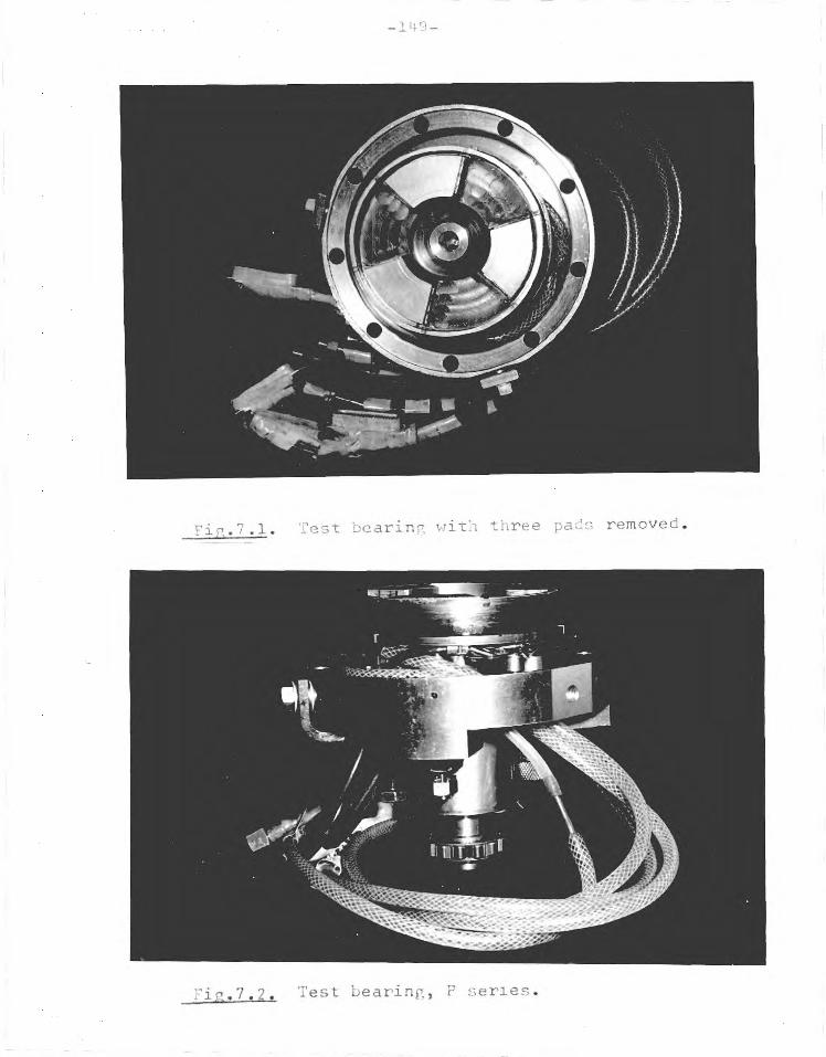
FiR.7.1. Test bearincT, with three pads removed.

Test bearing, series.

12.0° . • • . BA Ck SURFACE POINTS 0

INTEllittisbtottre Polv4T5

U 0

• • • szARtNag ir.lgtpArJa PONTS •

lkcrr4012. ItUAL'-rt0111/44

1Lerre R._

likerett I8P h= cp-se 42

a. 38 2 F-

34 34

30

26 • , ,

Fig.7.3. Pad temperature distribution, 960 and ld?.01oRPUM. aG" °C. 9Go statA as•bsc. 26

9P h

tt

TgERmocOuPLe S TAT toN.S,

SO

4-Ce

1-4 (.11

42.

- 3+

BACK SURFACE PC:ANIT 0

• I SITERMEIJIATE P INT% CS

BEARINGS SLR Pcorrs •

So

31 P 1-1=-2.1ESG

7 Rtrrocz= s4-

42

38

2e3PG.ss zo-roz.-4:7•7

34

•• • • . •

R.0-roll DtRECTIo1J

k

Z ZOO E Pm 2,-7 • 36-7 cb R PM SO° Fig. 7.4. Pad temperature distribution, 2200 and 3670 RPM.

30 30

• • • • •

X 20°

• rt

•

SO

ao

I0

0

PRE

SSUR

E P.

. S.!.

10

.../A

,v. ,;........... -__./ -... ___ . _.,-- „,/

,• ; , , •,„.. -,

IP, h.=.5.12 A 1

(LEAD

...., / ..----...-

ef,---. / ,..----'- -

..,. f

i% • -

i'i ij

2/2: A1=3.31

(TRA4 to

6

4

2

-2

-4

.152

PeE

SSuR

E P.

4

2

O

-2

-4

(LEAD

5

0

5 eY

t 02

- Ps ,., P4"

=P.

r

-10

-3P, Ar.2•61

1.........7- \

if „.....- .-- 4N\ \

/ 1 / 1 ,,, / ‘1 •

\ _,• • ...... I

I 6R /v.077

.\./

Fig.7„5„ Pressure transducer output, 960 RPM.

(map 30

ao

10

0

10

.0e...........N.

/ / ''' - -

\ ..

. 0 / \-

ii N.i

t ...../ .\ ......../ 1.- . -5/3 /7:: 0-99 — I • • A

CLEAli)

/ / e '

.....•".

•• • •••

• I

•••••.•‘

i I

/ /

0--... / \

SI •

1

1 1

/ ,--

•

''. ‘ • 1 ,1 '_• 1

li! .ti

I• i

/ I

, i

. /

..... /---‘. .'

%

, I i . i

lao

ex)

40

0

-So

PATV SWEPT BY TROISIDuC.EZ

-153-

too so Go 4o 20 o

-2o

7 P ht--075

,•• .0 • ‘

/ \

if. •.• 1

/ ....."1. • ..,.......... . %

J .ify•-•• ./

6P h=o75

too

80

Go

40

ao

0

-2o

9 P 11=0772

Fig. 7.5. Pressure transducer output, 960 RPM.

A

. ... 4.. ..... ,...,...

1 ,

1 t

,... .........„._

P h=9.40

\r

„.....),\.1

...----

% ' •N ....../. i

13 P h= 5.65

r N

I

f li

1

1

tf'

/ /

,

...•

\ \

i / i: I; . , .°Th

\

‘`.

J

•,i

1SP \-1%--

\ Vi

i .50

, , \? v 1

/ .

I,' 0

\ 1

)

14.1:5 11=2,4'5 •

.-, . 4

/ / / .

I . \ x ‘ ` 14 , t ti 1 la,

J ,\ 1

I

F ,/ , •

', „ . . . '-t I

Iiiri \ '....."

I

/(P h r•-• V GO

0

-5

to

0

5

5

5

Fig. 7.6. Pressure transducer output, 1610 RPM.

,0

5

0

4

-a

10

-154-

d.

0

-4 10

5

0

2.1) =-G.0

I ki

........ • / ‘

I / /', I '

..., /' , /1

S t

. %

k

k I:

li /

1

• ' \

\

nis

'

•

Go

4.0

0

-2o

18P tt 0.59

.--.

e / / •\ ‘ I 1

I /......,..,

/ i

I / I,1 1 ,ok.

• 1N\

j.v

ft I .

Wt 1;1 4/1/

1 V-.

/

125

l00

75

5o

25

0

-25

- so

PATI-1 SWEPT BY TRA.NSIbucEfe

-155-

-20

Go

40

20

0

..--- /

\.... • / , ,

f1

/

, -- .— ,- . \ ., LA lk

v • .v., ',-...--

17P hff-I•9

19 P h=O.7e,

Fig. 7.6. Pressure transducer output 1610 RPM.

-156-

20P hx5.G4-

f '‘

4 V% ,...41

...,

..._,/

22P h-4 .5.56

, ..... -... N..

A...

/

/

/

)

... .

\ .., /.

.....,

21P h=4.29

I' ti

..... A\ ,,..

rri.

, , v- ..................... --- ---- ) -\ .

/*-\\

/ / ,

/ A 1

/

I

1 I I

I

' 1

' \ \ 1

1 1 a 3

.

I .1

ird

)\ I I i 1 i

i I t

; r--,„

, ,„ *qv/

!„../

to

10

-to 23P h= 2.40

24 P h!1•50 25P kc Fib?. 7.7. Pressure transducer output 2180 RPM.

15

I0

5

0

-5

15

10

5

0

-5

-10

40

BO

ao

10

-10

40

30

0

-5

15

10

5

0

-5

15

10

5

0

-s

Va

..#• •• , / I / ,, It

.. .. . _

I #

/ '

•\

‘ ... t

/ . . • .

. . /,.

kr

/ ..„./.

. . ...te .

2GP hzocil

teN I

/ \

i• - -, 1

1 / // ' •

r /,' •

/,1 / /1

10

\ s ;7 \, ! 27 P h=0.83

100

8o

GO

40

2o

0

-do

-40

100 -157-

80

Go

4,6

2.0

a

-20

-40

—10

-5

0

aelP h.=- G-85 i!

II\ //h.

,,,, i \ ••• 4 .,.•ii

/ • \ "It.

."' ig. ...s.../a

• er ••.' . .......- _...•

3oP h=3.52. A II

0

• r

j_

0--".

i i • '1 '

. . . - - .. ..."•.....4'

i

2P h= 4433 • t

/I 4 .

• _,

\--e---- -••

31P 1.1=. 2•86 n A

rif\\ / : '

i'h•

...._./

2,. Is

to

5

20

'S

10

5

0

-5

20

(0

0

-10 Fig. 7.8. Pressure transducer output 3670 RPM.

4

2

P.51, 4

2

0 -'0

142 h = 2.48 V3P h = 3.65

-158-

-2

4 p h = 9.40

..—

••

p.• •... ....

4... •..a. re. ;,.. •••,.

..% ". / .s. .... .. .... ..' S % \

° , 4. I `% '• c„„ • --• - • , .„,,

...... / .

- \ /

.. s•-..,_....-,

P h = 6.11

..-

- .... ''" ....

‘ ••••• ..... ....

/ .--

/ •

s ,. N'• ..

• .. ............/.......

.N.•

.1. ... •. ... ... •. , 1

.

I

... \. •...„.

I0

5 3

0 -3

-5

/ /

N. N.

i

f - - .... •

\ /.'''..- ...,•.‘

ti 1. % \

1 s..... 1

. \ / ..••••-......

9`

..- -..„. / N

)

/ /

I 4

/ I

/ I

3 /11,/ ' '7, 1

i v.; \ ‘ I . I

I , ‘

a ‘.,'"---.. % \ % k1,,,..11

I.

G \ I

6

0

-3

15 P h = 1.92 P h = 1.62 • Fig.7.9. Pressure generation with boundary field subtracted

1610 RPM

-159-

7.3. Comments on experimental results

The removal of three pads to give greater circum-

ferential temperature differences and greater pad flexibility

was successful in allowing useful loads to be carried. A

larger number of tests werq performed at each speed than in

the previous series, to show the transition from negative to

positive load. This transition is best shown in Figure 7.10

which shows individual pressure transducer outputs as the film

thickness was successively lowered. Subsequent calculation's

show that the maximum degree of convergence produced by

distortion was of the order 10%. This figure could have

been exceeded in the absence of delicate instrumentation.

An analysis of distortion in Section 7.4 shows that

thermal distortion is always present, even in the most

lightly 'loaded' cases, but at large film thickness the

degree of convergence is too small to be effective and the

viscosity wedge mechanism predominates. Although the dis-

tortion alters by a mean factor of only 4 through each series

of tests,reduction of film thickness through an order of

magnitude increases the angle of oonvergence, and the

converging wedge mechanism begins to operate in opposition

to the viscosity wedge until fully positive loads are carried.

Temperature differences within the pad produce a con-

vergingadiverging film with the minimum film thickness

approximately 60% from the leading edge. A change of

the shape of pressure generation with speed is evident from

Figure 7.10. A similar change of shape was found by Neal

( 24)- Increasing speed gives a greater negative pressure

in the trailing section, although the distorted shape remains

approximately the same. This may be accounted for by the

decreased temperature drop in the trailing edge as the speed

-161-

is increased. Such a temperature drop exerts a positive

pressure influence in the trailing region.

This decrease of temperature drop may be accounted

for by consideration of hot oil carry over. The proportion

of heat transferred remains approximately constant with

speed (Figure 6.8), but the temperature difference tr-ts

increases with speed and the leading edge is swept with hotter

oil. Hehce this effect of changing pressure shape with

speed can be attributed to poorer cooling of the leading edge

with increasing speed, rather than better cooling of the

trailing edge at slow speed.

The effects of high local temperature gradients at

both ends of the pad are evident in the slight pressure drop

in the leading region (increasing temperature in direction

of motion) and the more pronounced, local pressure rise at

the extreme trailing edge.

Measurement of distortion

Pad distortion could be found from measurement of

deflection of the capacitance output as the transducer

traversed the pad. Corrections were made for the slight change

of dielectric constant with temperature. At large film

thicknesses distortion was too small to be recorded,

but became easier to measure as the film thickness was reduced

due to the inverse relationship between capacitance and film

thickness. Below a certain film thickness the capacitance

transducers gave reliable estimates of film thickness only

at the leading edge, due to the cavitation

phenomenon mentioned in Section 3.9. Hence only a certain

number of tests in each speed range were suitable for

measuring distortion.

Figure 7.11 and the accompanying Table shows the

DISTORTION VALUES

Test TmaxoC

3P 1.5 14P 2.8 15P 3.2 21P 2.6 22P 2.8 23P 4.0 30P 4.5 31P 5.1

C2 (Expt)

.018

.020

It noisy channel

1

.020 .037

-162-

08 0

tP 2 oc,

04

.0E

I I I I

KE.f 0 C2

A C_3 0 C.4.

..-- -.. .., - — -... ..... -.... r. ., .--- -... .... ---, cs ,---.... ce

A

A •

A 7.7

///°// ,..e./...,

./

Z -:

• 0 . :7

I

CI

I i I 2 4 6 5 A t TEMPERATURE DIFFEIZENCE cc

me x TPROUW-1 TWICKNESS oF PAD

FIGURE 7.11. Experimental distribution of distortion in pad

Distortion ins x 10-3 C3(Expt)(Theory) C4 (Expt)

.020 .018 .017 .029 .030 .024 .038 .037 - - - .018

.027 .030 .018

.043 .045 . .030

.045 .046 .029

.060 .054 .054

-163-

measured values of distortion which are plotted against

Atmax, the maximum temperature difference through the

thickness of the pad. It can be seen that maximum dis-

tortion occurs along C3 which lies closest to the centre of

the pad.

An analysis for distortion is given in Section 7.4_

The calculated values of distortion for radius C3 are given

in Figure 7.11 and show good agreement with experimental

values.

7.4. Theory

Calculation of distortion

Full details for the calculation of thermal dis-

tortion are given in Appendix 6. The strain at all directions

is assumed to be act, or ex = ez = e = x t. Strains

ex and e I which act in the plane of the oil film, are re-

placed by equivalent stresses and the deflection evaluated

for the resulting bending moments. The restriction of

thermal bending of the pads by the remainder of the bearing

plate was found to be small. Distortion for the third strain

e was found assuming free expansion. In general, thermal

bending was responsible for only one third of the total

distortion. Elastic distortions were neglected, since

the highest recorded film pressure was of the order 150 psi.

Ettles and Cameron (28) found that elastic distortions

in thrust bearings were usually negligible compared to

thermal distortions.

Figure 7.12 shows the distorted shapes for alternate

tests. The form of distortion is almOst parabolic about the

minimum film thickness, which occurs approximately 60% from the

-10

TRAIL. 0

10 A 0 ao

40

I 1 11 1 ill

41 .6 •4 .2

P

3e...,....----------''

-71,

9P

LEAD

eGo RPM

1 •8 •6 .4.

2.0 O

tO

m 40

z

Ili

-lo

TR.A‘L. 0 LEAD

Glo la PM 13P

ISP

153P

Go

23P asp

a-7P

• G LEAD

au:a0 RPM

-164-

-20 TRAIL.

10 $ qn 40 Z

z 60

Fig. 7.12. Distorted bearing shape.

-165-

leading edge. An important aspect of these results is that

the distortion is small compared to the film thickness. The

maximum degree of convergence reached was of the order 10%.,

A tenfold increase in distortion would put the bearing on an

equal rating with conventional thrust bearings. Methods

of attaining this higher degree of distortion and of

avoiding the diverging portion are discussed in the

conclusions to this Chapter.

Theoretical evaluation of pressure generation

The general method developed in Section 5.1 allows

for variations ,in film thickness. The solution for pressure

requires the integration of equation (A4.6) for the dimension-

less pressure A , where p = 12 L.,t1B/h2i x x*

and A - m 2.dx* K 1

o cg(x)j

tex)3 3 0.dx

where the variation of film thickness is expressed as

h = h ex). The expression

g(x) = (1 - -- 1—(1.82x*3/4 - 1.86x*) hi

was found to closely represent the distorted film shapes.

The temperatu're variation along the pad was represented by

t

where f(x)

f(x)

Figure 7.13 shows the agreement of these expres-

sions with the mean experimental points for each speed.

These expressions for temperature and film_

thickness were used in the computer programme shown in

= tfo Zitbf(x)

= 1.489x*5/8 - 2.869x*7 for N = 960 RPM

= 1.456x*5/8 - 2.216x*7 for remaining' speeds.

1.0

•Z

TRAIL 0

-166-

----.*NN\

•

.6 •G •Z

•-

4.,..1.489%.-

MEAN EXP. 1bGo "R.PM.

1

Wa

POINTS

,

2•869x.7 _

• —

1

1.0

•5

i(x) .2

TRAIL

-2

—

-1.4

(LEAD) %I

. .

_, , .

..,

0

.

1.456xda ".2'21G1

2200 RPM MEAN ;cot° RPM E%P. POINTS 1.

yx).

0 4

w

1..EAD)oc'

Fill. 7.13. Functions for temperature variation along pad.

N SERIES

Amax = - 10.7h- 2.03

P SERIES

+ 80.3h-2.77

-167-

Appendix A4.4. for the evaluation of X . The solutions of

dimensionless pressure are shown in Figure 7.14.

At large film thicknesses when the film can be taken as

effectively parallel, an overall positive pressure is generat-

ed. This is due to the greater temperature drop at the

trailing edge for this series of tests. This particular

effect has been demonstrated in Figure 5.3.

The increasing effect of distortion is clearly

shown. The viscosity wedge effect initially resists the

development of negative pressure in the trailing edge, but

this is overcome as the distortion increases. The

maximum generated pressure can be summarised for each case

with a power law. The tests for 3670 RPM have been omitted,

since the limiting temperature was reached before any sig-

nificant positive pressure was generated. The expressions for

the N series test results are included for comparison.

SPEED

960

1610

2180

where units

The rapidly

thickness is

h is raised.

is primarily

'thickness.

- 14.2h-1-74 +140h-3-11

Amax17.3h-1.625

+201h-3'2°

of p and h are psi and

increasing effect of distortion as the film

reduced can be seen in the high power to which

A close correlation of theory and experiment

dependent on accurate measurement of film

Amax

ins x 10-3 respectively.

Sample results of film temperature rise are shown

overleaf. Conduction to the bearing solids becomes of

major importance at low film thickness. Conduction limits the

temperature rise to an apparent maximum value at each speed.

At low values of film thickness the proportion of heat

removed by convection can be as low as 5%.

-168-

.6 .2

'X a

.2 -t

Fig. 7.14. Specimen computer results.

.,, sp

. \

..., P G P "s..

... -..

-BP IP

LEAD

ZGO RPM,

, a. .....m..pp OP

• •

/

/ r7P

N ‘ •

• • 1GP •

..... I 4 P ... -.. -4...i..

— ..... Q. P

LEAD

16t0 RPM.

11%104

TRAIL 0

2

TRAIL 0

-2

27c,

/ /

16". 26P\ \ \ A

\

/

/ /

/

/

..." • -

2SP

'—i--417.". N.

\ \

• • • 23P

... 22 P •

•

. -.

'4.... __ ...." /

I

• ,:

•E1 •6 .2 Xfs 0

LEAD

2150 RP.M.

to A -3

TRAIL 0

At 6C 4

2

0

. ..›...si.o2

• 1

960 R P.m. S • 1714‘ -es t

. .... ., .* / --..

N. _

e 2. ite \

. \`

1610 RPM, 41-o

0 . 1.0 8

-169-

1.0 •8 .6 4 •2. 0

Figure 7.14. Specimen computer results: Film temperature rise

Treatment for side leakage

All solutions were for conditions measured along transducer radius (3) and assumed an infinitely wide pad. The same problems for a full three dimensional

-170-

solution apply to this series of tests as for the last

series, except that the additional information of the full

film shape is required.

The side leakage effect was simulated by calculating

the pressure generation of a pad with a slightly converging

film and of finite dimensions. This solution was obtained

by relaxation arid compared with the infinitely wide case to

obtain local side leakage or attenuation factors.

The pressure generation from the relaxation case differs quantitatively from the actual case due to the

additional action of the viscosity and density wedges.

However the same coefficients of side leakage will apply

to each case.

An additional factor is that the areas of positive and

negative pressure changed with changing film thickness. These

areas could be found from the pressure transducer outputs.

Figures 7.17, 7.18, 7.19 show the positive and negative

areas for each test. The equivalent theoretical solution

was obtained by making the pressure on appropriate mesh

points equal to zero. Solutions were evaluated by hand

for the three different cases shown in Figure 7.15.

Inspection of the successive areas of positive and

negative pressure shows that the positive pressure area is

approximately parabolic in shape and of nearly constant length

equal to 0.75 of the pad length. The main change in shape

occurs at the outer edge, the zero pressure contour

expanding to the outer radius as the film thickness is

decreased. (Figures 7.17, 7.18, 7.19).

The pad was divided into a 6 x 8 mesh, and given a

I/ --

-- o6i to4 t-- t ,1/404. k lea

Lot 01.4- 1511'

,

0 tooS lop I o k

to t0 1°1

01- \es--

%.6 ‘13%'-".

1 1

S

-171-

l4"(POT14ETICAL FILM "rt4t0(.14E-S5 tO'

To--

---‘ •

\•••'"

10

to OM* sW aar* 16'

PE*" o$, op

VALUES OF 10 S 2E20 RIACWS Ps

6

i'l.---

--\ ei ---

Nr. , t-

s

oc X •,‘ 10C ZERO RADIUS

• '0 '- '0 0 /0 st,

0 )e. 4 ro

Y -A -r \ k

VALUES OF 'N 4105 B ZERD 1290:AUS C.

0 ---

rig.7.15. Hypothetical film shape. • ToP BC:4•1141)ARY

, KEY

1

01•12..A ReituS A - u 13 ,

,, . c

RANOS RA• ESA

I ZERO -

0 ,,

I

it • •

. /

?

I

I

I

.s tr

I

I

.6 a

I

I L

I

I 0,8

SID

E L

EAK

AGE

F AC

TO

R

.5

rao

•lo

50

bios

443

3o

?-o

(0

O 0.4- o.G. Fig. 7.16. Side leakage factor.

-172-

hypothetical film shape as in figure 7.15. The distortion

was assumed parabolic in the direction of motion, and the

amplitude of distortion was assumed maximum on the central

radius, changing parabolically to zero distortion on the

inner and outer radii. An overall increase in film thickness

of 10% from the inner to the outer radius was superimposed to

allow for dishing of the bearing plate. The assumed film

thickness at each mesh point is shown'in Figure 7.15. The

outer boundary of the positive pressure area was then assumed

to be at radius A (i.e. outer radius), radius B and radius

C. The solutions for dimensionless pressure A are shown

for each case. The side leakage factor for radius p3 is

shown below in Figure 7.16, this will naturally vary depending

on the effective position of the zero pressure contour.

For each experimental case, the mean position of

the outer boundary was found, and Figure 7.16 used to find

the side leakage factor. This was multiplied into the

infinitely wide (computer) solution to produce a theoretical

pressure for the practical case.

Three further points require explanation:

1) A similar solution was evaluated for the negative pressure

area, where the side leakage factor was found to be 0.91.

Since this area was proportionately much wider than the

positive pressure area, the curve of side leakage factor

becomes discontinuous in the region of zero pressure. How-

ever the pressures themselves are low in this region and

the discontinuity of the theoretical pressure curve is

not too great. A fair curve is shown in the correlation

of theory with experiment, Figures 7.17, 7.18, 7.19.

2) The relaxation solution was evaluated using the equation

and methods in Section 6.4.

-173-

3) The effect of boundary pressure around the perimeter of the pad was found using the analogue described in Section 4.4. This was added to the theoretical generation, to

produce a total theoretical pressure generation under the

pad along radius p3.

Correlation of theory and experiment

The theoretical pressure, treated for side leakage,

is compared with the transducer outputs in Figures 7.17, 7.18,

7.19. The contribution of the.boundary pressure field is

included.

In general the agreement is acceptable, particularly

as the theoretical pressure is strongly dependent on the film

thickness. In general Amax K x h-3, hence any errors in

measurement of film thickness are magnified.

The area of positive pressure is larger than that

predicted by theory. This could be due to a smaller trailing

edge distortion, or to the point of minimum film thickness

being further towards the trailing edge. Only in one test,

27P, is cavitation predicted.

The sharp pressure drop immediately beyond the

leading edge-suggests that the temperature gradient is

greater at the leading edge than estimated. In some cases,

This sharp pressure drop radically affects the agreement

of theory and experiment. A similar mechanism is evident

from the sharp pressure rise at the extreme trailing edge.

These sharp temperature gradients over a small distance at the

pad edge could exist without greatly altering the film shape.

This effect, which can only be reliably detected with

dynamic instrumentation in the rotor, probably occurs in all

other types of hydrodynamic bearing with a groove containing

cold lubricant. Agreement with theory is better at

higher degrees of distortion, where this effect at the

-174- 40

0

4o

2.o

0

20 .....

4 47 ei

..•• N

1 _

___ ..... ... ..c.if zi

___

it

GP 1.1= o•781

N /

/

A \

a

iti

i

1.

1

I /

/ 1410 -

--

. -

<1 A.7

Ai

X I 1

$r/ / iA / i

-

; • a .1./

/ / \

lek 4', 0/1 0/ •••.,

1 1 A / •

1••!=- 0 775

40

0

210

0

ao 45P= 0.76

7 P h =0.77 eo

TRAIL.

Fip. 7.17. Correlation of theory and experiment.960 RPM.

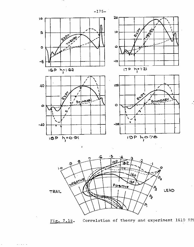
-le

Zo

to

O

40

0

-40

-175-

..- e ... ....

N %

.•• ..,"*.. l*C

7 . 0 / ...e. , 40 -r----

\ 44 I• ...• • .•

....- ... ---

1CoP 1-‘.1.62

I /

\ \ 1

40

74/ i

1 \

i'v V' bouNt...ro ....- t - -

it

/ Iv /

1t • .../

/

x ig

le3P

e...... N I

\

\1

jr „,.•-•0 449

40

4 , A./

/ % 1

%

\ - _ / 4--

17 P Inc 1.2.1

..- ” /

• \

1

t:15fC'/ I bOtbSC)1154.1—

1 tic / 1

\ / ..... IC 1

1 P c) 77

to

5

0

5

100

0

LEAD

Fig. 7.18. Correlation of theory and experiment 1610 RPI

-175-

40

-20

0

100

0

-100

....... 14 / /

• \

/( 6Dr ,. -

e or ./•`.-

2A- P hi- 1 52

.v/ ,010-•-•

axe • \

e Ci. %

1

_,... /

/V /

1 • ....... w

2.00 P h=o•93

/ „Or•-•

X

I I 50'

...... ..- -/

N N._/

/

Jr ri

2S P 11=1- 2.9

, \ lY 4,7 \

\

4r+0

1 -........\

... / /Y X

., /

It .,4

27 P 0-85

10

-(0

100

0

10

Fig. 7.19. Correlation of theory and experiment 2180 RPM.

/ /// // / rIS

P.Iacl. -7-20 Distortion of tongue type bearing.

-177-

leading edge is not so pronounced.

7.5. Practical implications of results

1) From the experimental evidence it is now clear that

"parallel" surface bearings operate by thermal distortion.

This evidence consists of measured values of distortion

(which agree with calculated values), and of the complete

change of generated pressure as the film thickness is lowered.

This process of change is perhaps better shown by the N series

tests.

2) A greater degree of distortion is required for the parallel surface bearing to be on a par with conventional thrust bearings The plain rectangular groove is not very effective in producing or allowing distortion. In general, a large number of pads is to be avoided since, for a given film thickness, the frictional generation would be lower. This would resQlt in

lower temperature gradients and hence less distortion. The

overall thickness of the pad and backing plate is not

critical, since any gain in thermal bending with a lower thickness would be lost with decreased fibre distortion.

Greater use could be made of thermal bending..

The machining of 'under cut

cooling grooves as in Fig-

ure 7.20 would allow far great-

er thermal bending. The deflection of such a canti-

lever is given by

.42 w 5 12 H Act

max

Although this tongue type,of

bearing could give adequate

-178-

distortion, the complexity of machining these grooves could

preclude its use, since a principle attraction of the

parallel surface bearing is its simplicity. It has been

suggested by Hall ( 29) that Michell pads with a line pivot

do not tilt at all, but operate purely by thermal distortion

as in Figure 7.20.

3) The shape of film induced by thermal distortion is not

optimum, since a negative wedge exists in the trailing

region. This could be reduced by insulating the back of the

pad from the cooling oil, as in Figure 7.21.

4) The sequence of events

during starting is not

yet clear, particularly

when starting under load.

The bearing responded quick-

ly to changes.of load, in

that there was a rapid

partial recovery of film

thickness after an increase

of load.

INSULATIOIX

, , , , , , , f , , ,

FiA."7-21 Insulation, of trailing edge

When starting from cold, the film thickness might

drop to a very low value. This would give high frictional

generation which would be rapidly adsorbed into the body of

the pad. At such a low film thickness, only a small degree

of distortion is required to form a wedge and the film

thickness would consequently rise. The use of boundary

additives in the lubricant would help to prevent scuffing

during starting. The instrumentaton was cons.„sidered too

-179-

delicate to try any transient tests of this nature. The

incorporation of a wedge in the leading section of the pad

by cold forming or scraping would aid load carrying during

and after starting.

5) Since the main criterion of successful operation is the

forming of a converging film by distortion, materials with a

higher coefficient of expansion such as bronze should be used

for the pad.

-180-

Chapter 8. Conclusions

Conclusions drawn from this work are divided into the following

sections:-

INSTRUMENTATION: MODE OF ACTION OF THE PARALLEL SURFACE

BEARING: DESIGN: CONDITIONS IN THE BEARING GROOVE:

FURTHER WORK. •

8.1. Instrumentation

1. Dynamic instrumentation mounted in the moving surface has

several advantages over static instrumentation mounted in each

successive bearing.

2. Piezo electric crystal transducers appear to be suitable

for measuring film pressure from the moving surface. High

crystal insulation is necessary, and the surface deflection

must be very small.

3. Capacitance transducers for the measurement of film

thickness are relatively simple to manufacture and position

but care must be taken to avoid movement from differential

expansion. Entrained dirt and air and cavitation can

interfere with the capacitance signal. An inductance system

would not be subject to these disadvantages, except for

metallic particles in the film, but would not be suitable for

dynamic mounting due to the layer of white metal of unknown

and probably varying thickness. Calibration of dynamic

gauges with the bearing in situ is not recommended due to

possible high spots on the bearing.

8.2. Mode of action of parallel surface thrust bearings

1. Six effects or theories have been put.forward in

-181-

past literature to explain the action of parallel surface

bearings (Section 1.1). All these effects are present in

the bearing to a greater or lesser extent, and contribute or

detract from,load carrying.

2. When the pad is truly flat and parallel, Dowson's pre-

dictions of negative pressure generation (23) are confirmed.

This may be confirmed qualitatively from Cameron's viscosity

wedge theory (10) using the condition that the temperature

rise on the bearing is greater than the temperature rise

on the moving surface.

3. In practice the density wedge effect is small compared

to the viscosity wedge effect, due to conduction to the

bearing solids. The large film temperature rises

necessary for a strong thermal wedge action are not attained.

In general terms, the film becomes increasingly non-adiabatic

as the film thickness is lowered.

4. The pressure ram at the leading edge is significant in

providing load carrying capacity. This could be one cause

of better performance at high speeds.

5. When the pad is flat and parallel, the form of the pad

temperature change in the direction of motion has a direct

effect on pressure generated. The sharp fall of temperature

at the trailing edge to below the leading edge value gives

a positive pressure loop in this region.

6. The change from negative to positive load with decreasing

film thickness has been demonstrated experimentally.

7. It is clear that useful loads are supported by a wedge

film produced by thermal distortion of the pads. Distortion

is always present in an operating parallel surface thrust

bearing. The distortion becomes increasingly effective as

-182-

the film thickness is lowered. Since temperature, dis-

tortion and film thickness are inter-related, (Section 4.5)

For an isoviscous system: p.411-4 approximately.

For a practical system: poch-3 approximately.

8. Temperature, or temperature differences,are of great

importance in parallel surface bearings, since temperature

differences directly affect both viscosity wedge pressures

and distortion.

9. When the pad is distorted and developing an overall

positive pressure generation, high temperature gradients at

each end of the pad still exert a pronounced local

viscosity wedge effect. These local effects tend to cancel

out as far as load carrying capacity is concerned.

10. Salama's theory of long wave undulation (8) is applic-

able in general terms only in that the shape of pressure

generation can vary from pad to pad as a result of slightly

differing individual film shapes. This could be produced

by varying temperature distribution as well as slightly

different degrees of initial flatness.

8.3. Design

1. Obtaining maximum distortion should be the main criterion

of design. In general terms, high distortion results

from large teTperature differences within the bearing. For

a given design high temperature differences (and high

temperatures) can be obtained by operating at high speeds.

2. The converging-diverging film obtained from symmetrical

grooves is not optimum for load carrying. Insulation of

the trailing edge (Fig. 7.21) could reduce the degree of

divergence.

-183-

3. More use could be made of thermal bending effects,

compared to direct expansion. A tongue bearing (Figure 7.20)

would have a high degree of bending distortion and could have

a performance similar to a tapered land bearing.

4. A relatively small number of large radial grooves is

necessary. Kettleborough (13) found the optimum number of

grooves to be four. A relatively large groove area at

the expense of pad area is desirable. A ratio of groove/total

area of 30 - 50% might give the best results. This

requires investigation. Grooves should be at least half as

deep as the bearing plate. This gives negligible restriction

of thermal bending. Deep grooves would give larger tempera-

ture differences. End restriction of the grooves prevents

oil starvation, and maintains cold oil in contact with the

pad edges, increasing distortion. Materials with a high

coefficient of expansion should be used.

5. The parallel surface bearing adjusts quickly to changes

of load, confirming Fogg's finding (2, Author's replies).

The sequence of events in starting from cold under load is

not clear. A taper at the leading edge would aid starting

and load carrying. The taper should be sufficiently

large so as not to be removed by small amounts of wear.

6. With design for maximum distortion an arbitrary design

figure of 100 psi could be used, which could be increased

for very high speeds.

8.4. Conditions in bearing groove

1. A relatively large quantity of heat can be carried across

the bearing groove to enter the next pad. This results in

the inlet viscosity to the pad being lowered by some unknown

-184-

amount from the viscosity of the lubricant supplied to the

housing.

2. The temperature of the oncoming oil is largely dependent

on the rotor surface temperature, which can be assumed appmx-

imately constant. - The negligible effect on heat carried over

of increasing the groove width by an order of magnitude tends

to confirm this assumption.

3. The leading edge ram effect can contribute to load carry-

ing. For design purposes the velocity ram could be taken

as approximately 0.4 x stagnation pressure.

4. Removal of the thermal layer would give a substantially

improved bearing performance, but would be difficult in

practice due to the high thermal inertia of the rotor.Rnife-

edged scrapers (Section 6.7) would remove part of the

thermal layer although partial reheating of the new lubricant

adjacent to the surface would be inevitable. Cole (19)

reported that supplying lubricant to a channel cut in the

leading edge of pad reduced pad temperatures. Rotor temperatures were not measured. Supplying excess lubricant

in this way would tend to deflect the thermal layer.

8.5. Further work

The following suggestions are put forward for

further work.

1. An investigation of the sequence of events during

starting under load.

2. An order of magnitude increase in distortion would give

parallel surface bearings a performance equal to conventional thrust bearings. Research is required into design methods

-185-

of increasing distortion whilst maintaining the basic

simplicity of the bearing.

3. A complete thereto-hydrodynamic analysis of the pad-groove

system. Hot oil carry over is at present one of the major

unknown factors in bearing design.

-186-

APPENDIX I.

BIBLIOGRAPHY

1. "The problem of the thrust bearing". H.T. Newbigin. I.C.E. Proc. V196, 1913-14.13t.II,p.223.

S.Z. de Ferranti, Discussion, p. 253.

J.M. Gibson, Correspondence, p. 257.

2. "Fluid film lubrication of parallel thrust surfaces". A. Fogg. I.M.E. Proc. 1946. V55, p. 49.

H.W. Swift, Discussion, p. 57.

3. "Parallel surface thrust bearing". A. Cameron and W.L. Wood. VIth International Congress of Applied Mechanics. Paris, Sept. 1946. Subsequently published in ASLE TRANS. Vol. 1, No.2, Oct. 1958, p. 256.

4. "An analysis of the parallel-surface thrust bearing". .M.C. Shaw. Trans. A.S.M.E. V69, 1947, p. 381.

5. "The hydrodynamical theory of film lubrication". W.F. Cope. Proc. Roy. Soc. V197. 1949, p. 201.

6. "On the solution of the Reynolds equation for slider bearing lubrication -VI, The parallel surface slider bearing without side leakage". Charnes, A., Osterle, F. Saibel, R. Proc. Roy. Soc., V214, 1952, p. 1133.

7. "On the energy equation for fluid film lubrication". Charnes, A., Osterle, F., Saibel, R. A.S.M.E. Trans V75, 1953, p. 1133.

8. "The effect of macro-roughness on the performance of parallel thrust bearings". M.E. Salama, I. M.E. Proc. 1950, V163, p. 149.

9. "Hydrodynamic lubrication of rotating discs in pure sliding, A new type of oil film formation". A. Cameron. J. Inst. Pet. V37, 1951, p. 471.

16. "The viscosity wedge". A. Cameron. A.S.L.E. Trans. Vol.1, No. 2, 1958,p.245.

-187-

11. "Theory of hydrodynamic lubrication in parallel sliding". W. Lewicki. The Engineer. V200, 1955, p. 939.

12. "Hydrodynamic lubrication of piston rings and commutator brushes". W. Lewicki. The Engineer. V203, 1957, p. 84.

13. "Tests on parallel-surface thrust bearings". C.F. Kettleborough. Engineering. V180, Aug.Sth 1955, p. 174.

14. "Temperature distribution within lubricating films be-tween parallel bearing surfaces and its effect on the pressures developed". W.B. Hunter and O.C. Zienkiewicz. I.M.E. London. 1957, p. 135.

15. "Effect of temperature variation across the lubricant films in the theory of hydrodynamic lubrication". W.B. Hunter and 0.C. Zienkiewicz. Journal Mech. Eng. Science. Vol. 2, p. 52, March 1960.

16. "'A review of hydrodynamic lubrication with particular reference to the Conference Papers". D.G. Christopherson. Proc. Conf. Lub. Wear. I.M.E. London. 1957, p. 9.

17. Authors Replies. D. Dowson. Proc. Conf. Lub. Wear. London, 1965. Unpublished at time of writing.

18. "New charts simplify design of pivoted thrust bearings". B. Sternlicht and E. Arwas. Product Engineering. V33, n8, April 16th, 1962. p. 124.

19. "Experimental investigation of power loss in high speed plain thrust bearings". J.A. Cole. Proc. Conf. Lub. Wear. I.M.E. London, 1957, p. 158.

20. Lubrication. A.G.M. Michell. Blackie and Son Ltd. 1950, p. 126.

21. "New theory for parallel surface'thrust bearing". A. Cameron. Engineering. V190, 1960, p. 904.

-188- 4

22. "A University's research for Industry". P.B. Neal, J.F. Wallis, J.P. Duncan. Engineering. V191, 1961, p. 434.

23. "Thermo-hydrodynamic analysis of the infinite-bearing., Part II., The parallel-surface bearing". D. Dowson and J.D. Hudson. Proc. Conf. Lub. Wear. I.M.E. Paper 5, 1963.

24. "Film lubrication of plane-faced thrust bearings". P.B. Neal. Proc. Conf. Lub. Wear. I.M.E. Paper 6, 1963.

C.M.M. Ettles, Discussion, p. 150.

25. "On problems in the theory of fluid film lubrication, with an experimental method of solution". A. Kingsbury. Trans. A.S.M.E., V53, 1931, p. 59.

26. "The velocity distribution in a liquid-into-liquid jet, Part 2, The Plane jet". E.N. Andrade. Proc. Phys. Soc. V51, 1939, p. 784.

27. "Verbesserung des Differenzenverfahrens von H. G8rtler zur Berechnung Laminarer Grenzschichten". H. Witting. Z.A.M.P. V4, 1953, p. 376.

28. "Thermal and elastic distortions in thrust bearings". C. Ettles and A. Cameron. Proc. Conf. Lub.'Wear. I.M.E. paper 7, 1963.

29. "Some characteristics of conventional tilting-pad thrust bearings". D. de Guerin and L.F. Hall. Proc. Conf. Lub. Wear. I.M.E. London, 1957, p. 142.

30. "Boundary layer theory". H. Schlichting. McGraw-Hill Book Co. Inc: 4th Edition, 1962.

31. "Theory of hydrodynamic lubrication". O. Pinkus and B. Sternlicht. McGraw-Hill Book Company. 1961.

32. "Strength of materials, Part II. Advanced theory and problems". S. Timoshenko. D. Van Nostrand Inc. 3rd Edition,l966.

-189-

33. 4th Report of the Research Committee on Friction. B. Tower. I.M.E. Proc. 1891, p. 111.

34. Trans. Cambridge Phil. Soc. W.J. Harrison, Vol. 22, 1919, p. 373.

-190-

APPENDIX 2. Initial theory

ITT

r a /////// //

e-' t

////1///11/ J 1/11/1/ ..141-11 ROTOR

TR. (CONSTANT)

FIG. A 2-1 Initial assumptions

The rotor temperature is constant = T r

The pad temperature rises linearly from Tt to Tr + La t

The temperature profile through the film is linear

Temperatures are expressed as T = t°C + a for convenience in the use of Sloth's temperature viscosity relation

_ C C

(t + m Tm

For the oil used C = .204, t = °C, a = 12, m = 2.5, = Reyns.

Then bearing temperature TB = T,(1 x A t) B.T1

and film temperature T = Tr - *(TR TB)

/1

T y

-191-

B. ' tx„ A substituting TB) T = Tr h T El - 1(1 - --

Lf,

R TTT

put [1 — —"-td(1 + At)] TR

and och = V

Substituting into Slotte's relation,

C ( A . 2 . 1) - « Y )m Trm(1

now C

Trrn SO

'Z r

(2.2)

( 1 - oc y ) m

(2.2) is an expression for viscosity at all parts of the film.

Pressure generation

Taking the same stress equation12 = y.

2u au or

()2„u mar )u dx (1 - coty)m• ?y2 (1 - °{y)m+1.4) y

Solving for u,

(2.3)

dx L 65,2 ay' cY

Substituting the general expression for viscosity, eqn. (2.2)

u - (1 - acy)n1+2 SIP C 1 ( 1 - 404 y ) m + 1

+ C2

(2.4)

(m+2) a.2 R dx (m + 1)

The constants C1 and C2 can be found using the boundary con-

ditions

at rotor surface y = 0, u = Ul

Q

-192-

at pad surface y = h, u = U2 from which

(m+1)(U1-U2 ) (m+1) [1 - (1 - ..(h)m+2.] dp

Cl = r

L(1 '<h)m+1 1-1n L(1 -och)/11+1-1](m+2) 2R0(2.dx

1 g.2 Cl C2 = U1 -

(m+2) 0( 2 2R dx (m+i)

The integral/ u.dy will give the oil flow Q

Q= rh

0

u.dy h

Q = [ (1 - pc y)m+3

.dxA2 4. C1 (1-0<y)m+2 - C2(1-o4y)

(m+3)(m+2) 0 3/R oc (m+2) (m+1) 0<

Substituting och = V gives

dp 1 _ y )m+3.j dx • 424

3 Tom-I-3)(m0.2)

ci ['( 1- 11)"2 - .4- a 0( [71 - (1 - Y )] co< (m+2) (m+1)

Substituting C1 and C2 gives a formidable algebraic relation which can be reduced to an expression:

Q - h 3 s_12 + h [m(Ui - U2 ) + Ifd (2.5) 12 2R'dx 6-4)

where

0

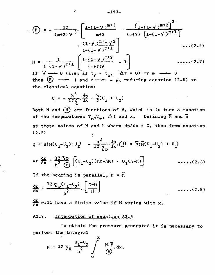
-193-

+

1

v )rn+1

i s

U2)

reducing

•••(2•6)

(2.7)

= 0) or m 0 equation (2.5) to

1•••(1.. V )M+1

1-(1- V )m+2 M

) 1a4.1

If 0 (i.e. then 0 1 the classical equation:

h3

(m+2)V if tr = to, Ll,t

and Pi -

+ S12 1-1(U = - + 12t 'dx 2' 1

Both M and 0 are functions of V, which is in turn a function of the temperatures To,Tr, At and x. Defining 11 and E

as those values of M and h where dp/dx = 0, then from equation (2.5)

Q = h(M(U1-U2)41y h3 aP

12 21:dx. = h(M(U1-U2 ) +

12 72r or IR = dx h3 ® F U1-U2)(hM-hM) + U1 (h-Rd

(2.8)

If the bearing is parallel, h =

12 )z r(U3.-U2) [M-Fi ] d h2

dx will have a finite value if M varies with x.

(2.9)

A2.2. Integration of equation A2.9

To obtain the pressure generated it is necessary to perform the integral

= - [1-(1- V )m+3 11-(1- V )ra+23 m43 (m+2) [1-(1-Y )ff)m+1]

(m+2) V 3. 2- 12

U -U TrB Then p = 12 1h22. At

vo

-194-

Now M and 0 are functions of V where

_ x Lit) Tr IPT1

TB- so dx = r .dV

At

The limits of integration are:

when x = x v = v

; whenx= Ov= 1 - = v

Tr 0

V =

or p = 12 U1-U2 TrB.

where A is a pressure parameter

A= r 0

dv - 0

or A = J1 - 2

13 may be determined from conditions at the end of the pad since p = 0 at both x = 0 and x = B. The integration was too

cumbersome to perform analytically, and use was made of the

Weddle six strip formula for numerical integration:

-195-

I = 177;2 5fl f2 ef3 f4 * 5f5 * f J where f represents the function to be integrated. This numerical formula is most accurate, the errors of the 6th dif-ference being at the eight or ninth significant figure of the evaluated integral. The integrals were evaluated to seven significant figures. Now

x /it v = 1 - -- L(1 + Tr 6 T 1 and varies between the limits:

when x = 0 V= V = 1 - Tr

Ti + pt.

x=B V = 1 ( R

Hence V decreases linearly with x. A typical experimental range of V is from 0.2( V 0) -'''411' 0.1( V B).

1 Values of® and6lwere evaluated for

= 0(0.01)0.10, 0.10(0.02)0.20, 0.20(0.05)1.00

and the integrals Jl and J2 were evaluated in each case from v = v to v = 0. These integrals were used to find the value of A for different spans of V (i.e. V - V) for a range

of different starting values ( V0). Table A.1 shows a range of values of MI® , V® and the corresponding integrals

J1 and J2 to v = zero. Sample values of A for v = 0,

vB = 0.20 are shown in a fifth column. The values of X are negative, giving a negative pressure generation. Figures 2.2 and 2.3 in the main text show the variation of local film pressure for a wide range of the parameters V/ 0 and ( vo - vB). For small values of ( V - VB) the pressure

generation is nearly parabolic in form.

-196-

Table A.1.

negative

1 V o

negative

J1 J2

v = .20--4P- 0

x 104

(neg.)

0 1.00000 .500000 .0000000 .0000000

.01 1.01255 .507766 .0050388 .0100628

.02 1.02553 .517103 .0101606 .0202524 4.361

.03 1.03843 .525859 .0153768 .0305725

.04 1.05207 .535013 .0206784 .0410232

.05 1.06534 .544031 .0260793 .0516137

.06 1.07999 .553901 .0315605 .0623329 10.540

.07 1.09468 .563870 .0371587 .0782159

.08 1.10918 .573828 .0428386 .0842255

.09 1.12592 .585045 .0486360 .0954042

.10 1.13981 .594862, .0545370 .1067395 13.124

.12 1.17200 .617099 .0666550 .1298393

.14 1.20534 .640353 .0792191 .1536090 11.539

.15 1.22294 .652638 .0856995 .1657782

.16 1.24051 .665012 .0922668 .1780588

.18 1.27633 .690483 .1058781 .2033162 5.031

.20 1.31671 .718904 .1199007 .2291547 0

.25 1.42359 .795596 .1577449 .2976279

.30 1.54591 .884721 .1996,868 .3717708

.35 1.6871 .989089 .246497 .4525315

.40 1.85434 1.113949 .2989567 .5409687

.45 2.04289 1.257704

.50 2.26911 1.431735 .4254442 .7457726

.55 2.53771 1.640881

.60 2.85917 1.894033 .5900459 1.0005084

.65 3.24602 2.201979

-197-

TABLE A.1 continued negative negative

1 M J V ® ® 1 J

2

.70 3.71431 2.578530 .8116838 1.32E9769

.75 4.28276 3.040025

.80 4.97274 3.605318 1.1170668 1.7567163

.85 5.80362 4.292248

.90 6.79952 5.122304 1.5484769 2.3395698

.95 7.96140 6.099260

1.00 9.28125 7.21875 2.1611595 3.1388640

-198-

Appendix 3.1. Test Oil Data

200°F 250°F 100°F 150°F

Thermal conductivity 0.079 0.078 0.077 0.075

B.T.U./ft.hr.°F

Specific heat 0.44 0.47 0.50 0.52

B.T.U./11).°F

Dielectric constant 2.256 2.215 2.178 2.138

2.3x1013 Resistivity 3.5x1013

ohm cms.

'2.4x1012 4.7x1011

Density .0313 .0307

lb/in 3

.0300 .0292

Viscosity curve shown overleaf

-19 9 -

AS

40

tr? 35 2 >••

of 0 so

U

25

3 20 f)

15

I0

5

0

Go 70 ao 30 .40 TEMP,

Fin. A3.1. Test oil viscosity.

Sd

• P I a P2 o P3 •

a

00/0.

. .

. "

I./

.."'" .

4

0

3

0

4

3 IA 1-• 0 0 0 4-

2 'rft-

.J 0

O

.200-

5

50 100

1 5 0 Zoo 25,0 500 350

P.S.I.

o P4 • ps

o

•

•

•

.00

i

50 100 IS0 Stoo 2.So 3O 350 Fi5z.A3.2.Pressure transducer calibra-

tion.

-201-

1

Wes( • •

, . I yv • LINE 0 ---

-14 60 -- - - - - - 6o }\

i• \ A ,\A

ACCEPTED COIZVE

0 V +

+ /Q0 SI-IIMMED

\'',..\ ` \\ \, •\

k......'. . **•••„ -..,-..,. -..A -- - -

--, -- -. _-... _

CI

I0

8

6

4 LL 0

a 2

0

AN k.IL1412 POSITIoN OF TRANSDUCERS

2 3 4 5 6

FILM THICKNESS )410

10

1) a 4

0 a 2

0

i • 11:2\r \`. \\\

‘\. wk• CURVE ACCEPTED

.44.0

a

Ns:•• lt.., ..--..

-...

C2

I 2. 3 4 FILM It•-,1$1(10 Fig.A3.3.capacitance gauge calibration.

a CII 4 IL 0 V

4

2

10

8

0

10

8

0

-202-

&

' ... CURVE•

_..

ACCEPTED

'....7"...... ........

......„,.. ------......

C3

o

2 5

F Kis.% Ti4tC.K.14E-SS t hicU ES x 103

d .\* t . \d. V

\iks

AC C.UIZNE

cEPTED

\ .4.,k \`‘.

.

\• No • %.4 Ill -

s.--. Iii ..... --

a

C4

3 4. 5 FILM T4itcKNEss iNsicioS Fig. A3.3 Capacitance

gauge calibration.

P I C

o F A

RA

DS

4

2

A

4 IL 4 0

10

8

IO

8

2

-203-

•

\ .

\ \ N C-LiVJE.

ACCEPTED

N \ .

A%• %*--........

..... -..,A

Cs

a 3 4 FILM Ti-IICKNIESS NS 0/

CALIBUATtot4 uSE WITH

C.t.)12•IGS FIRST TEST

Pai2 SWAIZNei

KEY Cl Ca

C3 C4._

— — — cs ______

c3

CI NA

\ -

....,N: .......4p6it

2 3 FILM TI-Itc.Kniess INS Ictos

Fi ci.A3.3. Capacitance gauge calibration.

PI c

o FA

RA

DS

4.

2

2s

ao

a

S

w tf. cr

to 2 w

ol

0 1- 5

0

•

Rotor thermocouple calibration.

KEY A P PENDN • MGNILSRION4 R.OTOR, A 141EATINI

• COoLIMail AIR REF

3- 4 TEMP=

TEMP-1'0'84S [4 Mrs+ 0-4(REF TEMP -16g

A

•

• •

• \'‘

•

. • .

. •

• .

5 l0 IS Zo 2s so (Zo-rosz - Ref) R.EANNG = A DA PLOTTED AS pl,+ O.4 C TREF- is)

35

/ / / / ///Tr

-205-

APPENDIX 4. Theory

A4.1. Setting up

FICA. A4-I . Film temperatures.

Initial assumptions

The rotor temperature is constant = Tr

The pad temperature rises according to the polynomial

Tb = TI iltb(138x5/8 - 1.82x8)

The temperature profile between Tb and Tr is parabolic.

Temperatures are expressed as T = toC + a for convenience in use of Slottes temperature-viscosity relation:

(t + a)m -Tm =

.10

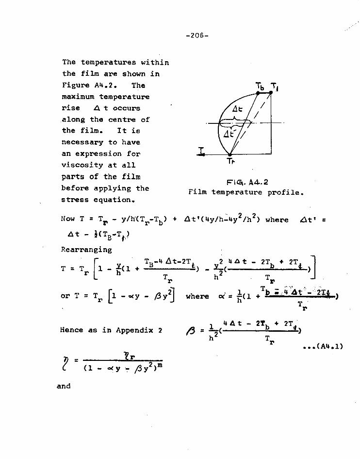
-206-

The temperatures within the film are shown in Figure A4.2. The maximum temperature rise Q t occurs along the centre of the film. It is necessary to have an expression for viscosity at all parts of the film before applying the stress equation.

A4.2 Film temperature profile.

Now T = Tr - y/h(Tr -Tb ) + att(4y/h- 4y2/h2) where LItt

At - i(TEr t)

Rearranging

]

lit - 2Tb + 2Ti )

TB-4 6t-2T L ) Y.—( 2 4

T= T [1 - 1(1 + r h Tr h 2 Tr T ' ' y2] 1 b ; 4 tit - 2T4 ) or T = Tr [1 - acy - where 0 i =

h"'-'0. 4' --- m

• Tr

4 A t 2T + 2'1' Hence as in Appendix 2

/r - (1 - acy -7 2 )m

and

= 12(

4) h Tr ...(A4.1)

m - 2$y) m E r( 0e + 2A y) (1 04 y /3y2)M+1 - (1 - y y2 )m+1

-207-

Substituting for '? and 47 in the Stress equation

.1.2 _ _ 2u u dx a y

stp . t r v 2.,"

m 2 r( co' + 2P y) u 2

+ .. „ (A4.2) dx (.3._ ocy,_ /,3y2 )m• ay (1- of y ... /3 y2 )m+1* ay

Solving for velocity u

- 11.2 ‘1 1, dx•Y + C1)(1 - ce y- A y2 )Mdy + C2

2 Taking M = 2 and expanding (1 - 0( y - A y. ) 2 gives

uZr dx = 1_12(1_2_23.y 3ee + y4 ( =„2_2/3 ) 50e/c3 .y6/32)

, 2 1 3 2 „ I 4 n Ty + C1ky-y + —y ( pc -2p ) + y cp + 5 /3 2 ) + C 2 3

The integration constants C1 and C2 can be found using the boundary conditions

y = u = U1 • y = h u = U2

putting = 8 = (1 + Tb 4 At - 2T1

Tr

4 „elt - 2Tb + 2T1) h2 = = T

-208- Then

(121,V2Q41(n2 26142nA 1.,(23 -fr(U2-111) dx- 7 4'- - ' 3-- 6- C - I 1 2 i 1 2 .

h(1-6,+-3(fi -26)+2G6*- ) , ..G.4-1(2-26)+106+16.) 5 3 5 C2 x U = 'r 1

The integral u.dy will give the oil flow Q

h Q = f u&dy

0

FiR 1 [.. 3 1 4 1 5 2 dx. -172Y 2*( bc -2/3 )4.13--6762a. +714-2.17

h

/3 2 111 o

1-2-y Co< -2N+rdy 20e/3 +-arly /3 0

1 4 2 5 6 a + ]h h

S.12-113r-6 20 .44.2-(g2- 15“ 2.1,)+190 dx T +

1 1 1 1!---01+--(02 -2(0+-06+1 + C1h2 31 12 10 306 + C2h

Substituting C1 and C2 gives a large algebraic expression

which can be expressed as

h 3 .12 - 12 2 r•dx*-`1

where

+ h 1 - U 2 )M

1 1 2 -26)+11.4?“4762) 0 = -12 (t--68+7017(0

(i-40401-26)+496462)(i-443+1-7(9?-26)+7+4562 ) (1-01+ 3((02-26)+i864462 )

...(A4.2)

7r

TrQ

1 3 2y2 -1,-57 24x

426

2y

flow Q. Put

Ul = U, U2 = 0.

(T) m , 122r.dx• +/ohU(1 + M) = /31J(1 + F)

-209-

M = (1 - 1 -9 + 12 (0

2 - 26) + 1-1096 + 10 62) 3

(1 - 1 + -(92 1 - 26) + i06 + -62 ) 3 5

To incorporate the effect of density wedge the mass flow

m = /0 Q must be taken as constant rather than volumetric

when 2 = 0

12 7rU a „, ="1 - + 17) 0 h2 fah

...(A4.4)

whence 5_12 dx

allowing h to vary with x, put h = h1 (1-d.f(x)) or h = h1 g(x)

where d 6 h1

...(A4.5)

)(

h1

2 [I x'

(x)]2()dxt_ e Le x), (l+m) r 1

3 dx] j 1+M r

o

x'

P = 12 DUB

[ (x)..1 /410 -1

...(A4.5) where x' = x/B.

The constants i;[(7,q (1 + I-71) = K may be determined

by assuming p = 0 at x = B. Before Q, 6 and hence M, 6H can be determined the frictional temperature rise Lt must

be evaluated.

A4.2. Frictional generation and conduction

The shearing of the oil film will produce a pro-

gressive rise in temperature in the x direction. Some

heat generated will be conducted into the bearing solids,

the remainder will be lost by convection. The heat losses

then

-210-

affect the viscosity which in turn affects the heat generated.

a. Heat generated

Work is done on the fluid by the shear stress r and the fluid either does or receives work against the pressure

gradient dp/dx. Since the pressures generated are comparative-

ly low and operating viscosities are generally high, the flow

work term is less than 5% of the first, using typical figures,

and is neglected.

Heat generated (Q =

For unit width dQ = dx U tr -1) x * hJ

x'

Qx BU2 ,)( BU2 .' hJ Lx dx 2 hJ mean.x ...(A4.7)

The heat generated at x = x is dependent on the pre-

vious viscosity, considered as 7) mean. Calculations show

that '9 can be taken as .2 m = x 4- 0.43( - )2!x) with mean 2

an error of not greater than 2.5% between Lit = 0 - 15°C.

b. Conducted heat

Referring to Figure A4.2

aT

il

4 At, Effective gradient at pad and rotor = ---1 ay y=0,11 h

a Heat conducted dOcond T k.2 dx.-45.-5 = 8k.dx. LI-0/h

from film -

put x' = x/B and assume At' = x'.( L t')max

= 8kB'At'maxxdx dQcond

-211--

Then total heat conducted from film between x' = 0 and x' = x'

Qcond = 4kB Atimaxx 42:/h ...(A4.8)

c. Convected heat

The difference in convected heat between x' = 0 and x' = xl is:

Qconv = [1 2(Tb +T r 3 ) + At' - i(To+TRd 2 /

At' mad

then

Qconv

d.

since TB =

I 421-11. C

To

2 .

+ AtB.f(xl)

AtB .

f(xt) 3 2

Heat balance

...(A4.9)

Heat generated between = Heat lost by conduc- + Difference in

x' = 0, x' = x' tion between x' = 0, convected heat

x' = x' between x' = 0,

x' = x'

whence

liAttmax)02 le /3Uhc [

[ At f(x') + 2x'41t' = BU

2k + B 3 max] hJ 'me and h 2

*

Rearranging gives an equation for 4 t'max

'max.Lx2 41tBf(x') max 3 K ymx' ...(A4.10)

where L and K are the parameters

L = 8RB K - 21th Q r.

/olUh2C Ah2JC

K is the adiabatic temperature rise and L approximates to the

ratio conducted/convected heat. Now 2m = 0.572 x + 0.43 ?0

will itself be affected by Z‘tmax and hence must be expressed

in terms of this variable. The viscosities 2 x and 9 so are governed by the mean temperatures at x' = x and x' = 0

respectively. These temperatures are:

-212-

• 2 T, Tx(mean) = 1(Tr+Tb) +ti Tr

+.,) 4 2 Tr Lit

TI ]To(mean) = 1(TI+Tr) = Tr [1(1 + T-.) r

Using Slotte's temperature-viscosity relationship

Zr. 2r lx - -T

$ II = C

r 4. _1 ) + 2 3 T

.411 M Tr r

The solution of equation (A4.10) for At' is max dependent on the power of m in Slotte's relation. Taking m = 1 will give a quadratic which can be solved for an

approximate value. This value can be used with Newton's

method of approximations to solve the cubic equation when m is

given the value 2. The use of m = 2 gives accuracy over

a wider range of temperature. Expressing Slotte's constants

P(1 +T m

TR

Cl C2 (t°C + a1)

1 (t°C + a2)2

1, equation (A4.10) can be rearranged as:

_ (B2 - 4AC)1 2A 2A

= [.667Lx3 + 0.44x dropping the points

as

F

For m =

•Lltmax

.where A

B = (tr+to+2a1+f(x)iltB)(05Lx2+0.333x)+1xLtB T f(x) 287Kx2 3

/(1+—T1) r.

[

1 Ay c,_,_0.430Kx 4. 1-1 "8"" i To

(1 + -f--) r

%Et

C =-(tr+to+2a1+f(x)atb

0.570KxTr

This solution will give an approximate value of be refined by Newton's method of approximations.

states that if ax3 + bx2 + cx + d = 0 and x1 is

max which can This method

one known

f(x1) X2 = X1 f( 1) ...(A4.12)

.6tn+1 =- n 3M(GIt)2 + 2B'a t + C' n . n

A'(4tn)3 + Bt(6tn)2 + Cl6tn + D' ...(A4.13)

-213-

approximate solution, a further approximate solution may be

obtained from:

Each further solution may be used in equation (A4.12) until them is satisfactory convergence between xn and xn+1. The solution

of Atmax i in equation (A4.10) for m = 2 may be expressed as:

where ,

A' = 2 [Lx4cr + 3-lc3 0-1

B'1 = [-J,c3V + 141tB.f(x).cr x2 + 2 -ax 2 V - 0.43Kx3or/ id

C' = [Lx2f + I AtBf(x) V x + 3x4E - 0.43Kx2 V /

D' = [i AtBf(x)E - 0.57Kx 0.43Kxi/ /4d

where

C' = 4 9T 2 r

T

Tb 2(1 + --)/3Tr r

T132 Tr'

1(1 + T-2) 2 r

Three iterations were found to give convergence

within 1%. The computer programme contained instructions

for eight iterations. The centre line temperature rise 41t

is required. This may be obtained from at' max

tp

E = 4(1

=

-214-

Lit = x1 -41trtnax At6f ( x ) ...(A4.14)

Knowing 41t, Q and 6 may be found and hence M and 0 , allow-

ing a solution for pressure by the integration of equation

(A4.6). For parallel films the film thickness function g(x),

where h = g(x), may be taken as unity (Equation (A4.5). The

variation of density with x is required. The density-

temperature relation for the oil used is

= 0.03190 - 2.461 x 10-5(t°C - 15.6) lb/in3 ...(A4.15)

where tm = mean film temperature at x

tm = 2(t1 + tr) + 17-.41Ib.f(x) + iilT ...(A4.16)

A4.3. Solution

The solution for pressure requires the integration of

equation (A4.6) for the dimensionless pressure A , where

p = 12 zrUB/h1 x A and

x' : x'

A . 1 + M

[g( xi.3 2.dx' K I 1

[g(x)] 3 p0 .dx?

o o The constant K was found by integration between x' = 0

where A = 0. The six strip formula by Weddle was used (Section A2.2). Each integration requires the solution of

At at seven equally spaced points, giving Q and 15, and

(Also g(x) for non parallel filmns).

A was evaluated at x 0(0.1) 1.0 for each experimental case.

The computer programme for the Elliot 803 is given

in the following pages. The input for each case was:

thence M,

-215-

D(J) tr D(J + 1) A tB DCJ + 2)

+ 3) a1 D(J + 4)- a2 + 5) d D(J + 6) L D(J + 7)

-216-

A4.4. Computer Programme

SETS J11;1-1NLil SETV A(6)ZC1)PQ3(9)CD(312)E(9)F(2)GC16)RT(7)U(7)SVC6)WC2) SETT SQRT SE 17', 21 17)TITLE

• VISCOSITY WEDGE PLUS THERMAL WEDGE PLUS TAPERED WEDGE CUTAWAY 1)J=1 4)READ D(J) J=J-1-1 JU:IP UNLESS J=3 1)L4 J=1

15)H=5 11=0 L=0 1=C 2)CYCLE A0=0:.166666667:1 SUDR REPEAT AO JU1IP 510 6)1=0 CYCLE A0=0:.01666667:0.1 (Set cycles of x in steps of SUDR 5 1/6th) REPEAT AO JUiiP L10 7)1=0 CYCLE A0=0:.03:333333:0.2 SU R 5 REPEAT AO JUMP G10 6)1=0 CYCLE A0=0:.05000000:0.3 SUDR IZEPEAT AG JU,,P 5)1=0 CYCLE A0=0:.06666667:0.4 SUER 5 REPEAT AO JUiP 513 10)1=0 CYCLE A0=0:.03333333:0.5 SUDR 5 REPEAT AO

JURP 018 11)1=0 CYCLE A0=0:.10000000:0.6 SUER 5 REPEAT AO JUHP G13 • 1?)1:=0

-217-

CYCLE A0=0:.11666667:0.7 SUUR 5 REPEAT AO JUI:P L.,13 13)1=0 CYCLE A0=0:.13333333:0.3

5 REPEAT AO JUNI' 013 14)1=0 CYCLE A0=3:.13000000:0.9 SUBT-', 5 REPEAT AO Ja.P L10 5)01=AO'AO 02=1:31eEl B1=82 ,81 D1=51*A0 52=Sf]Ri AU D3=ST B2 (Evaluate 03=SRT B3 f(x), pad 03=033 *B2 temp.) „Ulf) IF i' , 9L20 01=2.86931 D3=1.410933 C=33—B1 JU1:P L,21 20)D1=2.216<-31 B3=1.456*83 C=63—B1 V 21)Q0=DCJ)+DCJ+1) A2=2e;DCJ-1-4) Q0=CIO — A2 Ci 1=DCJ-1-2)*C Q2=q0-1-Q1 C,O=A0A0 G3=Q0*.5 Q3=D(J+7)*Q3 (214=A0/3 Q3=C3+eg c13-ci3',tcl2 c5=0,4tel 1 c3-Q3-1-015 15=Q0*Dc3-1-3) Q5=.287tcZ Ci6=DCJ) —D(J-1-4) Ci7=DCJ+1)—DCJ+4) CiO=CIOM Gi 8=i+Q8 Q3=.50Q8 Q5=Q5/Q0

Q4=. 25*C-1 1 Q5=A0*D(3=3) Q5=.43*Q5

4 (Find variables .10 5130,C' for At'

max,

Slotte m=1)

GO=2*Q3 -- Ct5=g5/Q3 Q4=CR4 —Q5 Ci4=Q4*Q2 . c,s6=Ao*G7 G6=Q6*6(3-1-3) Q6=.57.Q6 G4=Q4 —G6 05=00*A0 G5=Q5*Dcd4.7) G5=.667*G5 Q6=.444*00 05=05+06 Ci6=4*G5 Q6=q6-q4

Q7=G7—G6 Q7=SQRT q7 Q7=Q7/Q5 Q7=.50Q7 Q6=G3/Q5 q6=.5*Q6 Q6=G7—Q6 E9=c16 U=DCJ1-1)+DCJI-5) M=Q0*Q0 Q1=9*G1 G1=4/Q1 G2=0(3+2) *C G3=DCJ)+0(3+5) Q-4=Q3-1-02 C-15=Q4/Q0 Q5=14-C-i5 cl6=2. ,,Q5 Q7=3*Q0 c6=c16/Q7 G4=Q5e,Q5 04=.25*Q4 Q7=c13 /GO Q7=14.Q7 G7= 0,7 ci7=Q7*G7 Q0=AO*A0 Ci3=Q0.6 A0 C-15=Q0*Q0 Q8=Q5*G1 U=Q3 4sOCJ-1-7) Q9=C13 0G1 Q9=.66666667*G9 08=Q3-1-C2,9 0;9=0,3 *0,6 0,9=0,9*0(3+7) C;10=.5,02 Q-10=Q101 Ci10=C.10*Q0 C,11=0,0 *0,6 Q11=.6666.660*G11.

:(First value be

max

(Find

1\

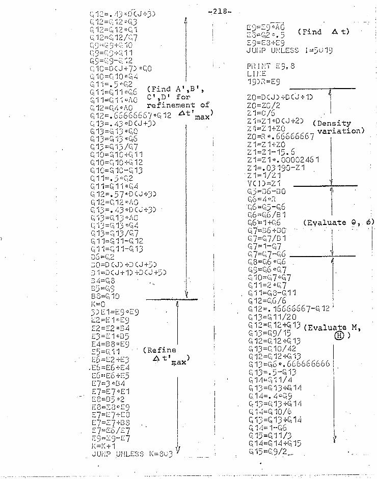
G 12=.43-1-j) 6il2=C112,:'Q3 Ci12=C;12Cil C'; 12-C'

rr

0,9=11 C9=6i9-C 12 MO=DCJ-1-7)0,0 C;10=010 ; C4 C1 11=.500,2 Q11=Q11,;,Q6 (Find

-Q11=1-111*A0 C e sp i for

Q12=C-1,4*A0 refinement of

Q12=.66666667112 t'max) C113=.43DCJ-1-3) C-113=Q134'u cil3=Q136 0,13=13/c17 Q10=010-1-Cil1 Q10.--C,10-W2 6i10=010-Q13 Ci ll=.5*02 Q11=M1tGA Q12=.57*DCJ+D) Q12=Q120A0 Q13-.43*DCJ+3) cil3=M3A0 Q13=Q14 Ci1:3=C113/017 • Q11=Q11-Q12 Cill=011-0113 D6=Q2 00.0(J)+0(J1-5) 1-31=DC,J+1)+DCj+5) 1734=U [315=c6 88=Q10 =0

3)E1=E9*E9 02=01 E9 2`2='2 *u4 E3=El*D5 E4=B8E9 E5=011 (Refine E(6-E2+E3 t )

.E6=E6q-E4 r;ax

EC=E6+E5 E7=3B4 E7=E7o01 E0=55 *2 Er3=E8*E9 E7=E7.4-E0 07=07+05 E7=E6/E7 E9=E9-E7

JUMP UNLESS ic=8C;3

E9=EDA0 (Find A t) •

E9=E8-FES) JUilP UNLESS I=5u19

PRINT E9,8 LIFE 19)2=09

ZO=D(J)+DCJ-1-1) zo=z0/2 z1.-C/6 2:1=Z1.9DCJI-2) Z zo--R.66666667 variation) 1=21+ZO

(Density

Z1=Z1+Z0 Z1=Z1-15.6 Z1=Z141.00002461 Z1=.03190-Z1 Z1=1/Z1 VC1)=Z1 Q5=06-DO

fr,-;):(f;171 Q6 C16=Q6/B1 G6?-11-Q6 C17=06+Da (Evaluate Q7=Q7/91 Q7=1-Q7

G u=6,606 4

00=0,7,',017 m1=2*Q7 Q11-u-c1 11 Q12=Q6/6 012=.16666667-Q12 Q13=Q11/20 Q12=C1124-G,13 (Evaluate M, 0,13=Q9/15

) 12=012 +G 13 Q13=Q10/42 C1 12=0,12+G13 Q13=Q6*.666666666 0:13=-5-013 Q14-Q1 1 /4 C1 13=C1134,Q14 C1 14=.4Q9 013=Q134-0114 Q14=C1 10/6 GT3=Q13+M4 Q14=1-Q6 0,15=Q11/3 Q14=0,14-1-Cil5 Q15=Q9/2_

B=B+A3 2=0+U4 B=B+A5 D=S+U6 B=0/20 D=D A1=5";:,V1 A3=8*V3 A5=50/5 B=V0i-A1 (Weddle D=B+V2 S=3.4-A3 B=B-1-V4' B=D+A5 13=BiN6 3=0/20 P=B Q=C +D JUMP IF M%1C16 S=Q/P PRINT S,8 LINE 16)F2=St- P F2=b2—F2

PRINT F2,8 (Print LINES 2 L=L+1

.H=H+1 JUMP UNLESS L=10 .GN J=J+8 N=N4-1 TITLE

(RETURN).

TEST NO. PRINT N,2 LINES 4 JUMP UNLESS J=3130)15 STOP START 17_

Integration)

-219- C114=Ci 14+Q 15. M5=M0/5 C714=M4+0,15 (2115=c4 /3 C15=.5—c)15 c116.-11/12 ci15=c115-i-c;16 0116=ci9/10 cii5=Q154-ci.16 cii6=MO/30 (2,15=c115-1-0,16 TC 1) =M5/Q14 i(I)=—Tct) u(1)=Tc1)4:M3 ucl)-G12-1-u(1) u(1)=uCI) ,,12

icI)=TCD/uci) UCI)=1/uCI) Vc1)=ucIpo./CI) 'u0=A0*A0 tjo=u0,,U0 UO=WO*1:86 U1=SQRT AO W2=SC]RT 411 U1=WI*W2 W1=W1*1.82 411=41 1—U0 W1=DCJI-8)1 NO=1—U1 W1=WO*WO 412=1,11 *U0 TCI)=T(I)/W1 UCI)=UCI)/W1 VCI)=VCI)/W2

1=1+1' EXIT 18) N=11+1 Al=2T1 A3=6 *T3 A5=5 *T5 B=TO+A1 B=C-FT2 B=B+A3 B=3+T4 D=B+A5 B=B+T6 B=B/20

Al=13U1 A3=6 *U3 A5=5*U5 B=U0-1-A1 B=B+U2

(Film thick-ness

variation)

(Weddle Integration)

Isoviswo R 6opog

s 114 ER1A13 -

+1, 0 Lir(ER

StliirACX

FIG. A S-1

-220-

APPENDIX 5. Mass and heat transfer in groove

A5.1. Solution of the varying viscosity boundary layer

A boundary layer

of thickness S will be formed in the groove, with a layer of hot oil, thickness

GC ti adjacent to the rotor

surface.

Put e= 6-/S

From reasons in text, es-

will generally be small, of

the order 0.05 - 0.15. An

excellent approximation for the

isoviscous velocity profile was obtained by Polhausen (Schlicht-

ing -(.30) p. 243), who assumed a polynomial:

u* = ay* 4- by-.„2 + cy*3 + dy*4 where u* = u/U, y* = yAr

Applying the conditions:

1) ( aviA/ ay*) ,= 0

2) ( 0)0/ yfel)]. = 0

3) 21,1*/ Dy*2)0 0.

4) (u*)1 = 1 yields u* = 2y* - 2y*3 + y*4 ...(A5.1)

For the variable viscosity case in Figure A5.1,

the viscosity varies through the thermal layer by a factor N,

where N = 2 sr Condition (3) implies that inertia

forces are negligible at the rotor surface. For a viscosity gradient at the rotor surface, this condition could be

modified to the full term y( 2 au/ cry) = 0. However

with typical viscosity gradients this leads to negative

velocities in some parts of the boundary layer. In general

the thermal layer is very thin and a solution for velocity

-221

can be obtained if the condition a/ 3/( E 4)1.1/ 3y) = 0 can be

extended for a small distance from the surface to include the

thermal layer.

The viscosity varies through the thermal layer in some

unknown way, but it can be shown that the viscosity ratio N,

which can be found experimentally, has a greater influence on

boundary layer formation than the actual shape of the

visoosity profile.

Considering the thermal layer only, with the rotor

surface as origin, consider two possible viscosity profiles,

plotted in Figure (6.4)

(1) 1 + oc (1 - r/rt)2

(2) k

whence N = 1-* 4,c' 1 + cx(1 - r/rt)

6

All velocities and distances are cons idered dimensionless i.e.

u* = u/U, r* = r/R, y* = y/S . The prime * is omitted for

brevity. blow within the thermal layer

a/ a r(i au/ a r) = 0

• • • 3u/ 3r = A'.1/t

u=A7-".dr

Substituting the first viscosity profile

u= Afl + 0((1 - r/rt).dr + C

then u = A(r - 043St (1 - r/rt))+ C

put r = rw uSt = A.r + C

r = 0 1 = -4A oc re / 3) + C

It will be shown that A = 2u* ,St • • C = u* at L1

2 S

-222-

Hence list = 1/(1 + 26t(1 + oc/3)

for profile (1)

u t = 1/(1 + 26;t(1 + 007)

for profile (2)

Values of u*(St for the two profiles, with rt = 0.1 and varying

viscosity ratio are shown below.

(1) (2)

N me u* u* St St 2 1 .790 .814 3 2 .750 .795 4 3 .714 .777 5 4 -..682 .760 6 5 .652 .745

For profile (1) For profile (2)

au/ a r = A(1 +,.<(1 - r/rt)2) au/ Or = A(1 + oc (1 - r/rt)

6)

. . . a Yu ,)o = A( 1 + ) = p

for both profiles

and ( u—) r (st A.

The original Polhausen. conditions may now be

applied to the remaining (isoviscous) portion of the boundary

layer, provided that the two separate profiles are matched

for slope and value at St. Shifting the origin such that

r = 0 at tl let the polynomial be

u = u st + ar + br2 + cr3 + dr4

Then au/ ar = a + 2br + 3cr2 + 4dr3

and e2u/ er2 = 2b + 6cr + 12dr2

-223-

Condition Equation

(uo = u 6t)

a+b+c+d=-u et

a + 2b + 3c + 4d = 0

2b + 6c + 12d = 0

2b =

a = A

Solving yields A = 2u dt (required for solution

in thermal layer) and

u = u st [i. - 2r + 2r3

The two profiles in and above the thermal layer are

now continuous.

A5.2. Thickness of varying viscosity boundary layer

The thickness of the boundary layer is not yet known.

The application of boundary layer theory, for example by Schlich

tine (30), p. 241 gives the boundary layer thickness as

= (2K/s)2( xi? U)2

1 where s = f f(1 - f),dy

K = f'(0)

where f is the dimensionless velocity polynomial, Expressing

S and x non dimensionally as 6* = cr/h, X = x/h, the

boundary layer thickness becomes,

6.* = (1 -or)-1(2K/s)1(X/Re)1

where the viscosity of Reynolds number corresponds to 2 r-Evaluating the integral 's' over the whole boundary layer? and

expressing the boundary layer thickness as 6 = D(X/Re)2

1.

2. (

ul =

au/ = 0

3. ( 2u/ar2)1 = 0

4. ( a2u/ ar2)o = 0

5. ( 1.1/ er)o = A

-224-

the coefficients for the two viscosity profiles, with a typical value of rt = 0.1, are

N

1

D(1)

-

D(2)

-

(= 5.83 ./TT) Disoviscous 6.83

2 9.6 9.5 8.26 2 11.2 11.7 10.1 4 13.6 13.5 11.6 5 15.4 15.12 13.0 6 16.916.6 14.3

The thickness coefficient for the isoviscous

boundary layer using the free stream viscosity )2 s is in eluded for comparison in a third column.

The complete viscosity profiles for N = 2, 4, 6 are

plotted in Figure 6.6 for the two different viscosity profiles.

Figure 6.5 compares the isoviscous profile with the profiles for varying viscosity. The isoviscous solution for thickness gives a good approximation for the 99% thickness of the vary-

, ingviscositycasesi.e.,6*F5.83(X*./7)Uh)2. It can be shown that for a range of 'vanes of r and N, S*g110 1.16S*.

t 99

A5.3. Velocity ram pressure

Consider the control

volume 1, 2, 3, 4, 5 in

Figure A5.2. Assuming)

1. = ty = 3/26-99

2. The rate of momentum 'Li

transfer through

1-2 can be found

using the iso-

viscous solution.

3. The velocity pro-

file at entry to the

/ / / i / / /5

Ale

F-1. A 5.2

-225-

film is given by t1 = (1 -(y/h))

4. p12 = p23 = 0. 5. A total force F acts on 4-5 in the x direction.

Equating forces and momentum in the x direction

A M = M12 - M45 - 7 15' 'ex + F

2 ,112.dy 4.Ef u2.dy r.3 S/2 + F

Evaluating integrals, OM = /OU2h (0.183 X* - 0.333.) /g

Shear stress term: if /7= 2 , then using velocity

solution for profile (1), it can be shown that

= 2U 2s/ C(1 + ar + 20 (1 + *03))

whence shear stress term T = 2.58U ?s/ El + d + 26 (1 + oc/3)) Then F = Am + T.

known but A

as y = y/

form p/p

The form of the pressure profile on 3-4 is not

0J P454 = F. Expressing distance non dimensionally Ly, let the expresson for ram pressure be of the = 1 + a; + by2 + 43 + 44, applying the conditions

at y ly, p = 0

= 0

F =

dp/dy = 0 d2 p/dy2 = 0

dp/dy = 0

p/p0 = 1 - 6;2 ty

p.dy = 0.6

A3 + 8y

ply =

A4 - 3y

0.9499Po

at y gives

now

whence p0 4-7U2(0.203-0.370/5* 9V U

.2.87 1+Cf +2cr(1+-!--)] 3

-226-

A5.4. Viscous ram pressure in 450 chamfer

h = 110 + —17(h1 - 110)

h or h = ho(l+mx/B) where m = ho-- 1

Then using —2 d 6Lii~dx c h3 = 020 ifus,

6lly l+mT/B 1 dx h2 l+mx/B)3 (l+mx/B)

Integrating with respect to x

= 6U 71 B 1 (l+mi/B)

mh2 [(1+mx/B) 2(1+mx/B)2

0

p

i he / / / --.,--- I

+

/7i/

put x = Bs

whence C = P = 0

l+mx/B 1

2(1+m)2 (l+m) put 7 = 0, x 0

whence 6Ut B1 po. ) I'max 2

.mho (1+m)2 l+m

Sternlicht (31) gives a solution for high angle sliders

which indicates that the use of simple theory gives errors

of the order liDyq. This is adequate for an approximate

correlation of results. Tables 6.1, 6.2 shows results

for two different groove widths. Fair agreement is attained

for the larger groove.

-227-

A5.5. Hot oil carry over

Approximate analysis

P.1G. 45-3 Distribution of velocity and temperature

in groove. Assumptions:-

1. The rotor remains at constant temperature.'

2. The temperature profile can be represented at any point

by the expression t = Lit(1 - yi st)a, where 'a' varies

with x. A family of curves for different values of

'a' is shown in Figure A5.4.

3. The principle of conservation of heat will be applied as:

Heat flow Heat flow Heat considered

in groove from pad from rotor.

4. Velocity profiles at entry and exit are linear.

5. The temperature through the film at exit is constant, i.e.

a = 0.

6. A simpler standard velocity profile, u* = 1 - 1.5y*+ 0.5y*3

will be used, which compares well with Polhausen's

solution u* = 1 - 2y* + 2y*3 - y*4. See Figure AS.S.

, 0 Lor=i-I•ski to,z3 ips )44 ett.1-2e42.-r-

lal\L\9•-

.2 .4 .6 •8 1.0 u*

0 .2 .4 •Go TEMP.

1.0

.4

-2

Gh

5h

4h

3h

0

-228-

FICA. A 6-4 Functions of FIGI• A5-5 Comparison of

t = 1-(y/ t ) a standard velocity profiles.

Solving for power 'a

Putting t = 4t(1 - y/ 5t )a where 6t = tr tinlet tr is and 0 = 1 - 1.5y* + 0.5y*3, then S* = 4.64(X/Re0

1) Heat flow in groove past any line AA', Qf

Qf =,Pc St

0

dt ut.dy = .ocU Atf (1-1.5y/E -0.5y3/63 )

0

(1-y/ S t )a .dy Evaluating the integral

cr 1.5 cr2 3 64 Qf =?cdtUha a+1 (a+1)(a+2) . (a+1)(a+2)(a+3)(a+4)

or Qf = p c dtUh (S*.f(e, cr) (1)

-229-

2) If heat .conducted. from rotor surface = Qc

Qc = k.x(-577) = k4attp3X o

It can be shown that E and 6* increase approximately as x2, then -a- * =

3 s t

s a(x)2 t(x) hence

Qc = k AtX(a/ S t) (2)

3) Heat outflow from pad, 00

Q0 = 0.5fUch At (3)

From assumption (3)

Qf = Qo Qc

Then pc AtUh *5*f (a, ) = 0.5,0Uch At + kAtXai St

X a f(a,tr) = [0.5 + Pr . Re V'

0r, cc*, X, Pr, Re, St are known. pq can be found by iter-

ation using Figure A5.6 in which f(a, o ) is plotted as a

function of a and cr.

Entry of oil into pad

Since 6 = 20h 200h, the oil entering the

following pad will be moving at a velocity very nearly U.

Let Tm be the mean entry temperature, then

ih

0.5h tm = hits,/ (1 - yi t)a.dy

2 (5* whence --12 = t 1 - (1 - 1/2 6*)a+1

At (a+1)

since [a) is known, tm can be found. Then entry temperature

100

w

1•0

0 1 •001

10

I- Ca, cY)

PIGt. A5.6 SOLUTION FOR FUNCTION [g - .3•Cr4 as I (at) (a42) (b.1.00.4:1)6,3A3W244

•01 .a

-230-

VALUES .oe c)

0o .

Cr

0 b

-231-

into next pad

tentry = tinlet + tm

Correlation between theory and experiment is shown

in Tables 6.3 and 6.4 for two different groove widths.

TEMP.

-232-

APPENDIX 6. Analysis of pad distortion

Two origins of distortion are considered. The

first is thermal bending of the bifilar type produced by

longitudinal stresses. The second is 'fibre' or free

expansion in the thickness of the pad. The analyses of both types follow.

A6.1. Thermal bending

A circular pad (or

inner plate) is considered

mounted in a solid circular

backing (outer plate).

The inner plate

has a partially restraining

edge moment Mb constant over

the whole surface and a vary-

ing thermally induced bend-

ing moment.

The deflection from

each of these bending moments

may be superposed. Pi AG-I

Thermal bending of circular pad and backing.

Inner plate

Assume the strain at all points is o< t, i.e.

ex = ez = at.

Consider a stress f to produce this strain, fx = f = f.

Then e = e = f) = ac t x z t

Whence f = EcKt/(1 )

Assume a linear temperature gradient

t/21t = y/H Hence f = Exy6t/( 1- > )1-i

H -233-

Then total force = f.dy = EceditH/2(1-)2)

Now distance of centroid from Neutral Axis = H/6

Hence bending moment M = Evc 4tH2/12(1 - y )

If At is this function of x, At = Atmax(1 - 2b- )

EacH241t

(x,z) = (12(1 - max - Then M 2b (A6.1)

For a plate subjected to two equal perpendicular bending moments

, d2w r dx dx2 D(1 + y )

(For small deflectio9)

Where r = local radius of curvature

C slope

w = deflection D = flexural rigidity, EH3/12(1 - V 2)

'24 1 E <4112 A tmax (1 7E) dx • D(1 + ) 12(1 - ) Hence

(A6.2)

Integrating twice for deflection gives two integration con-

stants which are both zero since p • = 0 and wo = 0.

Rearrangement gives

vl, ac Atmax x2 x3

H 2 12b

(A6.3)

The negative deflection due to the partially restraining edge

moment Mb must now be considered. Applying equation (A6.2) for a constant bending moment Mb gives

Mb.x2 2D(1 V ) (A6.4)

Mb is not yet known.

Outer plate

Timoshenko (32 ) gives a general relationship

-234-

for plate theory (p. 94, equation 90)

d d "cc x x 111) 15 (A6.5)

where V = shearing foi,ce at any section due to applied load.

Ettles and Cameron ( 28) found that, in general, thermal

distortion was much greater than elastic distortion in thrust

bearings. Hence taking V = 0, and integrating twice;

9V F1.x/2 + F2/x

now SU = 0 at x = a, hence Fi X2)

(x (A6.6)

For a bending moment acting along a radius, Timoshenko gives the relation (P. 93)

M= Do dx [AC +

where Do = flexural rigidity for outer plate

hence if M0(x) = bending moment in outer plate

2 _2 1 F1

Mo(x) c Do [1 + Ay) + 9 ( 1 - )

o putting x = b, Mb = D

2

F1

2 [(1 + ay)

- b2) (A6.7)

The integration constant F1 may be found by equating the slopes of the two plates at x = b

Flb a2 -I- (1 - --2- of

max 3) = .4b

whence

F1 3 a Atinax( ___ a 2 2' H ‘‘b' -

-1 (A6.6)

The deflection w may now be found using equations (A6.3), (A.6.4), (A6.7), (A68 ). Substituting the following values

for the variables:

-235-

a 1.5 ins.

b

0.75 ins. OC 1.2 x 10-5 per °C

E = 30 x 106 p.s.i.

= 0.3 H.=, 1.0 inches. Ho = inch. hence D. = 2.75 x 10 lb in

Do

= 0.342 x 106 lb in

and putting x = b to find wt, the edge deflection

wt = 0.248 x 10-5 6 tmax inches (A6.9)

N.B. The distortion without the restraining bending moment

Mb is only 14% greater. The distorted shape is almost

parabolic.

Form of distorted shape

Value x/b % distortion parabolic point

(Centre) 0 0 0

0.2 5 4

0.4 18 16

0.6 39 36

0.8 67 64

(Edge) 1.0 100 100

A6.2. The effect of asymmetrical temperature distribution

To find if the form of distortion is radically

altered with an asymmetrical temperature distribution, the

following simpler case is considered for comparison purposes only.

1. The pad is not subject to edge restraint.

2. The problem is two dimensional.

-236-

3. The temperatures on the front and back faces may be

represented by the expressions:

tf = tfo + Qtb(1.69x* - 2.19x*7)

to = Litu(3.42x* - 2.92)0

2)

where x# = x/t

through the pad is linear

is proportional to

If the temperature profile

and assuming that the bending moment

temperature difference, then

Stress f = Eoct

f = Etx(tf - tu)y/H

H Force = f f.dy

F = j Eoc H(tf - tu )

Then bending moment about

neutral axis

M = FH/6 = EaH(ti-tu)/12 ..(A6.1)

Using the relation

M = -EI d2w/dx2 and integrat-

ing twice yields an expres-

sion for deflection w. The

integration constants may be

integrated by putting w = 0 at x Ol t

The expression for deflection becomes

Fig.A6.2. Case for asymmetrical temperature

distribution

-237-

ocx2 w = H fl Atb(0.282x*-0.0304x*7)- tu(0.570x*-0.243x*

2))

m/x a— (-2t fl-0.252 Atb + 0.327 iatu) (A6.11)

Proceeding in the same way for a symmetrical

temperature distribution At = AtMdX (1 - ) gives

w = - — 01 t2 A -- Lat (1) 2 - 1 x*3 5

max 12 12) (A6.12)

The two deflection curves (A6.11) and (A6.12) are

compared for a particular case P18. Substituting approp-

riate values gives the two deflection curves shown in

Figure A6.3.

.4 0 7- 11) Z• 0 1

0

J•02

• 03

As-04° , '

F Differing distortion with symmetrical and asymmetrical temperature distribution.

-238-

A6.3. Direct expansion

If the strain at all points is N: t, then

ex = ez = e = « t. The effects of the longitudinal

strains ex, ez have been considered in sections A6.1,

A6.2. Referring to Figure A6.2, the total local dis-

tortion relative to the neutral axis is given by

=

H rI e .dy = a f t.dy

iH

put t = to H + I(tf - t u)

whence E = 0: H(Itf 8 + u) 8

Expressing the temperatures as functions of x:

tf = tfo + 4tbg(1)

to = Atug(2)

and substituting H = 1.0 inches

oc = 12 x 10-6 ins/°C.

gives 6 = 4tbf(1) + lAtuf(2) + 4.5tfo ins x 10-6

where the evaluated functions are, for 960 RPM

...(A6.1

x* f(1) f(2)

(Lead) 0 0 0

.2 2.61 0.53

.4 3.92 1.22

.6 4.45 1.49

.8 2.02 1.33

Equation (A6.13) gives total deflection relative to the

neutral axis, and hence gives finite values of distortion

at the leading and trailing edges. For finding the film

shape, distortion relative to the leading edge is required.

-239-

Examination of the experimental temperature distribution showed

that the temperature profile at the edge of the pads was non

linear. The thermal distortion at the edges was estimated

to be

Leading edge So = 2.4t10 ins x 10-6

Trailing edge t = 2.0 Lltu ins x 10-6

Hence the distortion relative to the leading edge may be

written

S = Atbf(1) + lltuf(2) + 2.1tfo (A6.14)

and at the trailing edge gt = 2.0 A tu - 2.4tfo

The distortions from thermal bending and direct expansion

are superposed. Complete distortion curves for alternate

tests are given in Figure No.(7.12) and values of leading

and trailing edge distortion for each test are given in

Tables 7.1 and 7.2.

Copy 2

Paper 7

THERMAL AND ELASTIC DISTORTIONS IN THRUST-BEARINGS

By C. Ettles, B.Sc. (Eng.)*, and A. Cameron, M.Sc., Ph.D. (Associate Member)*

The various distortions that affect the performance of thrust pads are studied. Equations are derived for elastic deflections assuming a circular thrust pad centrally pivoted with a conical pressure distribution. The thermal distortions are also analysed and these, under normal operating conditions, are found to be much larger than the elastic deflections. A design method is advanced which enables the minimum film thickness to be calculated.

This analysis is applied to some experimental data for the thrust-bearings of the Grand Coulee dam and for a ship. The agreement is most satisfactory. Arising from these considerations some modified pad construc-

tions are suggested as a means of limiting pad thermal distortion.

•

INTRODUCTION AND OBJECT A NUMBER of recent papers on thrust-bearings have considered the distortions the pads suffer under load (e.g. Baudry (')t and de Guerin and Hall (2) but do not give any theoretical analysis of the results. Other papers concern themselves with the mathematical analysis of distortion without attempting any correlation with prac-tical results. In this paper the authors study all the pos-sible significant distortions both elastic and thermal of thrust pads and attempt a quantitative solution of the problem, leading to a generalized method of design.

Surprisingly enough, despite the great technical im-portance of thrust pads, this type of analysis has never (as far as the authors can find) been carried out before. In order to simplify the analysis centrally loaded pads are considered. This has a further advantage that it emphasizes the importance of distortion, as without it no load is carried, and allows an important class of bearings to be subjected to quantitative analysis and hence to design methods.

The authors have been able to test their conclusions using some experimental data obtained on big thrust-bearings.

The equations giving the various distortions are all contained in Appendix 7.1. The MS. of this paper was received at the Institution on 30th

August 1962. * Lubrication Laboratory, Mechanical Engineering Department,

Imperial College, London. References are given in Appendix 7.111.

Notation B b C1, C2, C3 D - D1,

D2 , D3

E

G H h K,, K2 L M p

Q1, Q2, Q3

S r

w U X x cc1

8 '1

Pad span in direction of motion, in. Support radius, in. Constants. Flexural rigidity, EH3/12(1— v2), lb.in. Constants. Young's modulus, lb/in2. Strain. Modulus of rigidity, lb/in2. Pad thickness variable. Film thickness, in. Constants. Pad breadth, in. Bending moment, lb.in. Pressure, lb/in2. Constants. Outer radius, in. Stress, lb/in2. Temperature difference, degC. Surface speed, in./sec. Load, lb. Deflection, in. Shear force, lb. Deflection parameter. Radius, in. Linear coefficient of expansion per degC. Shear strain. Overall deflection centre to edge, in. Mean film viscosity, lb sec/in2.

58

V

T

Subscripts max

0

Poisson's ratio (0.300). Shear stress, lb/in2:- Shape, radians.

Maximum. Inner section. Outer section.

C. ETTLES AND A. CAMERON

3 2

/ // / / / / / / / / / / / / / /

RUNNER

EFFECT OF PAD DISTORTION The simplest and most popular method of pad support is shown in Fig. 7.1.

Load is transmitted through a circular button in a recess in the back of the pad. The load is applied on a spherical protrusion on the back of the button, leaving the pad free to tilt to its optimum position.

Assuming initially that the pad distorts to a spherical shape, consider the three pad profiles shown in Fig. 7.2.

For given conditions of load, speed, viscosity and bearing dimensions there is an optimum degree of pad curvature to obtain the greatest film thickness at the minimum point. The optimum profile (2) has a greater film thickness than profiles (1) and (3) which have a lesser and greater degree of distortion respectively (Raimondi (3)). Hence it is desirable to design a pad such that the distortion obtained at the running design condition approximates to profile (2). For a given pad configuration, decrease in minimum film thickness requires a decrease in pad curvature to retain the optimum profile. However, in practice a decrease in film thickness from increasing load results in increased curvature giving profile (3). Hence the bearing becomes progressively more unsafe as the load is increased beyond profile (2). For spherical films Raimondi gives the optimum degree of distortion as 0.60 of the minimum film thickness.

ELASTIC DEFLECTION The following simplifying assumptions are made in the calculations of distortion:

(1) The pad is circular and of uniform thickness H. (2) The oil film pressure distribution is symmetrical

about the centre and conical in form.

LOAD

\\\\\\\ \\\\\\\\\\\\\\\\\N

RUNNER

Fig. 7.1

Fig.- 7.2

(3) The pad is supported along a narrow annulus of radius b.

(4) The pad is assumed to be elastically homo-geneous. The distortions are elastic.

The validity of these assumptions will be discussed later. Equations are derived for deflection w at any point relative to the annulus radius b where w has origin. In the deflection calculations the effect of a variable button radius (b) is taken into account. It can be seen that for (b/r) nearly equal to unity, the pad will distort to a concave form, for (b/r) nearly equal to zero a convex form will result. At one intermediate value the deflections at the edge and the centre will be equal and overall distortion will be minimum. Deflection downwards is considered positive (Fig. 7.3). The deflection at radius b is taken as zero. Four typts of elastic distortion are considered.

(1) Pure bending. (2) Shear. (3) Differential pressure bending. (4) Fibre crushing.

These are considered in turn. After considering elastic distortions the most important thermal effects will be treated.

Pmax

b

Fig. 7.3

THERMAL AND ELASTIC DISTORTIONS IN THRUST-BEARINGS 59

(1) Pure bending In Appendix 7.1 the expression for a conical load on a circular pad radius r of thickness H supported by a rigid annulus of radius b is given in two parts where the radius x is less or greater than b. For (bIr) ratios in the region of 0.5, bending will tend to give positive deflections both at the centre and the edge. For lower values the bending moment at radius b can be sufficient to produce a negative deflection at the centre. For large values of (bIr) the loading outside b is small compared to that inside b, resulting in a negative deflection at the edge.

In practice the thickness of the pads is made approxi-mately 0.25 of the pad diameter. Experimental data were available for pads having this' Hlr ratio (see Fig. 7.4), which is a typical value. For plates of this thickness the effect of shear deflection must be considered.

The expressions for bending deflection are: x greater than b

7,0 =

pniaxr4 r ix

r

) 2

K1— b 2

D [k 0 K2]

where .

= 0.015 62 02 = 0.0112 02+0.0417 ln

+0.0104-0.004 44 03

rx2 b 2 b K2 = 0.04171n (-2 ) +0.004 44 G) —0.004 42

+0.0104

EH' —v2) D 12(1 — (flexural rigidity);

v = Poisson's ratio. x less than b

Pmaxr r /b2—x2\ 2° — D LQ1 Q2- r 2 pa

where

Qi -= 0-0156 (14 — 0.004 44 ( 7.) 5

Q2 = 0.0156 (r-b) 4 —0.004 44 (b) 5

Q3 = 0.0313+0.04171n (1+0.0112 (-12

(2) Shear The expressions giving shear deflection are produced in Appendix 7.1 and are: x greater than b

[(x3 b3)-F 1 ln (x2 b21 — HG 6r2 4 b 2.672-2 x less than b

W

prna.r2 r(b2—x2) (b3—x3)1 HG L 2-67/.2 6r3

The effect of shear is to produce a positive deflection at all - points. For pads of standard thickness the effect of shear

can exceed that due to bending.

0-87 0.50 0.17 1.00 11,1.2-57 0.33 0.33 0.67. vaid

1101"4111111/4 01101W414rAW

AP 4W

(3) Differential pressure bending A third type of deflection is considered resulting from the differential pressure applied to both sides of the pad. One side of the pad is subjected to a continuous distributed pressure which is counteracted on the reverse side by a 0-50 load on a line of radius b. The distributed pressure will

0.67 cause a lateral expansion to take place on the surface 0.33 giving convex curvature of the pad. This will result in a

positive deflection at the edges and a negative deflection at the centre. The expressions for deflection derived in 0-87 Appendix 7.1 are: x greater than b

For I-11r = 0.513; v = 0.300; w = px maxr

Fig. 7.4. Elastic distortion of a conically loaded plate with ring support at radius b

prn„„H2r2 [ tx2-21,2) (x3 —1,3 b3)] 0.0137 r 0 005 18

x less than b

w --Pmaxii2r2 [0.0137 (b2 -2x2) 0.005 18 (b3-3

x311

V

(4) Fibre crushing A fourth type of deflection is considered in simple crushing of the longitudinal fibres by the direct effect of oil film pressure. The maximum effect is at the centre, being the point of maximum applied pressure. The effect falls progressively to zero at the edge. Relative to the surface

w=

Amax = 1500 lb/in2

6,

6 in(=2r)

60 C. ETTLES AND A. CAMERON

at radius b, this results in a positive deflection at the centre and a negative deflection at the edge. Deflection due to fibre crushing is : x greater than b

w tx—b\ 2E Pm" r

x less than b H Ib—x\

= 2Epmaxl r The combined effect of these deflections can be reduced

to dimensionless form as shown in Fig. 7.4. A non-dimensionless deflection X is defined as

w E r Amax

The deflected surface of the pad is shown in dimensionless form for various values of (b/r). It can be seen that the magnitude of the support rig radius has considerable effect on the overall distortion. Fig. 7.4 is drawn for an (H/r) ratio of 0.513, experimental data being available for this value.

Selecting as an example a value of (b/r) = 0.33, the relative magnitude of the different types of deflection are shown in Table 7.1.

The last three types of deflection can be taken as thick-plate effects. It can be seen that they form a major part of the deflection.

Fig. 7.6 shows the elastic deflections of a specific case shown in Fig. 7.5, which may be taken as typical. Fig. 7.6 is of some interest since it shows the conditions at starting. When the bearing is started, the pads will be at a uniform cold temperature and hence unaffected by thermal distor-tion. Assuming that an oil film forms under the pad, in the critical stages of starting the deflections will be only of elastic origin. Raimondi has shown that a concave pad profile on a centrally pivoted pad is relatively far less efficient than a convex profile. Fig. 7.6 shows that use of a (b/r) ratio of more than 0.5 will result in a concave profile during starting, leading to possible failure. A (b/r) ratio of 0.5 is to be avoided since this gives approximately equal deflection at the edge and the centre, resulting in very low lift. The best ratio appears to be 1/3 which provides sufficient but not excessive deflection at the edge.

The necessary assumption of line contact at the annular support radius b leads to discontinuities of slope in a small

Table 7.1. Relative magnitude of different types of deflection

OIL FILM PRESSURE

Fig. 7.5

region x = B. This assumption will have little effect in areas remote from x i= b.

THERMAL DISTORTION The friction of the oil film between the pad and the rotor produces heat, a small portion of which flows into the pads producing a temperature difference between the front and back. This thermal gradient results in convex distortion. The assumptions of temperature distribution in the pad are shown diagrammatically in Fig. 7.7.

The temperature difference is assumed maximum at the centre reducing linearly to half this maximum value at the edge of the pad. If the temperature difference is assumed constant the equations (discussed later) show the rim deflection is greater by only 20 per cent. Little information is available as to the form of the temperature profile through the pads. Elementary heat transfer theory would give this to be linear. However, it is possible that there is a metallurgical effect at the babbit—steel interface giving a discontinuous profile at this point (Barratt (4)). Moreover the pads can be considered 'thick', with heat conduction taking place from the sides. These two effects

(xIr) 0.83 0-50 0.17 0.17' 0.50 0.83 1.00 0.67 0-33 0 0.33 0'57 1.00 3 i I I I 1 I I i I I 1

VA LU ES(bl 0

". 0 0

.F:

z 5

Centre, per cent 0

Edge, per cent la

Bending —133 b.10

60 0

Shear +173 41 Differential pressure — 27 13 Fibre crushing . + 87 —14 15

100 100

5

0.5 0.33

017

0.0

Fig. 7.6. Elastic distortion only

BACK

5

10

DEFL

ECTI

ON

— in

. x 1

O

15

a At At = 10 degC. (4,-)

0.83 0.50 0.17 017 0.50 0.83 1.00 0.67 033 0 0-33 0.67 1'00

VALUES (b/r)

1.00 0.83 067

060

0.33

0.17

0.00

b At At = 20 degC.


Fig. 7.8 shows the effect of three different thermal gradients on the specific example shown in Fig. 7.6. The curves drawn show the effect of both thermal and elastic distortion. Fig. 7.8c would give the most realistic case for a medium-speed turbine bearing. For (b/r) = 1/3 and taking the temperature difference from front to back of the pad to be 30 degC, the various distortions at the centre and the edge may be tabulated (Table 7.2). The sign convention is that a positive distortion means the pad surface has moved away from the counter face, i.e. the oil film has got thicker.

(x/ 0

r) 0.83 0.50 0.17 0.17 0.50 .83 1.00 0.67 0.33 0 0-33 0-67 1.00 LI I i i t I I I I i r

VALUES (olr)

0

Fig. 7.7. Assumed distribution of temperature difference

could cause the profile to be non-linear, a fact confirmed by Warner (5), who measured pad temperature at three points through the thickness of the pad, one point being in the babbit metal. Warner joins these points to give a profile approximately cubic'in form. For the purpose of calculating thermal distortion a parabolic gradient has been assumed. Although this choice is arbitrary, the effect on thermal distortion is small. A linear gradient gives a rim deflection of only 2 per cent greater, while a -5

) cubic profile gives a deflection some 8 per cent less. Two types of thermal distortion are considered, first that due

0 0 to induced bending moments, which is by far the larger, and secondly direct expansion of the pad thickness.

Two thermal distortions are considered: z 5 0

(1) thermal gradient distortion; (2) direct pad expansion. LL w 10

The expressions for them are derived in the appendix and merely listed here.

15

(1) Thermal gradient distortion

x greater than b wo

W - H [0.500 ( r2 ) 0 0943 ( x3 r311] -5-

- 0

-17 0.33

0-50 0-67 0.83 1.00 0-83 0.50

a dt,„a x2 b

„r2 2 Too o•e7 0.33

017

_

VALUES (bIr)

x less than b -

a dt,„a„r2 7 0 0 W - -

H [0.500 ( 2r2x2) -0.0943 (--b3-1 1 2.2 E _ x - . I _

5 _

. (2) Direct pad expansion 01-

x greater than b , , - LL Lo

W . a d t

4in „,„H /x -

r b\ 0 10_

k ) _ _

0-67 0.50 0.33

0.17

0-0

x less than b 15 a dtma jl

4 e At At = 30 degC.

Fig. 7.8. Elastic and thermal distortion

62

C. ETTLES AND A. CAMERON

Table 7.2. Distortions at the centre and the edge

Position Distortion, in. x 10 -4

Elastic Thermal Total

Centre . 0.2 —1.2 —1.0 Edge . 2.0 6.8 8.8 '

It can be seen that distortion from thermal origins forms the major part of pad distortion. The overall deflection of some 1 x 10 -3 in. for b/r = 0.33 is large as applied to its effect on pressure generation when com-pared with the minimum film thickness which will be of approximately the same order. The expressions for the six different types of thermal and elastic distortion have been grouped together in Table 7.5 in Appendix 7.1.

DEVIATIONS FROM THEORETICAL ASSUMPTIONS

Tilting of the pad has been neglected in calculations of distortion. Tilt of the pad causes a small shift in minimum film thickness from the centre towards the trailing edge. The point of maximum temperature difference undergoes a similar shift. The maximum film pressure would also occur at the trailing side of the centre but the resultant of the film pressure must pass through the centre for centrally pivoted pads. When considering a pad with maximum pressure and temperature difference displaced from the centre the problem becomes unsymmetrical and more difficult to handle. It is known that the point of maximum temperature is not far from the centre (d'Achkov (6)). A slight displacement of, say, 4r, would have little effect on the edge deflection of the pad.

The temperature difference between the centre and edge of the pad results in hoop stresses which would tend to distort the surface of the pad. Calculations have shown this distortion to be of a second order effect and hence it has been neglected. Deflection of the opposing rotor surface has been neglected. The rotor would also be sub-ject to thermal and elastic distortions to give a convex shape when viewed from the pads. Assuming the pads remained flat, this convexity would tend to give a spherical film with the axis normal to the film and passing through the pivot. However, the effect of rotor distortion on bearing performance would be small compared to the effect of pad distortion for the following reasons.

The deflected shape of the rotor, would tend to parabolic rather than spherical form. The pads would lie along a part of the deflected curve remote from the origin where the increase of deflection with increasing rotor radius would be approximately linear. Hence, although the pads would tilt inwards, the relative deflection of the rotor surface when viewed from the pads would be small. Moreover this distortion would be partly neutralized by the effect of film pressure on the rotor surface under the pads. This would tend to produce a concave depression in the opposite sense to the overall rotor deflection.

Pads of circular form have been considered rather than a square or sector shape owing to the comparative ease with which circular-plate theory can be applied. Trans-formation of the results for square or sector shaped pads for design purposes is dealt with in the next section. However, any deviations from the circular form will naturally take place at the pad edges where both tempera-ture difference and pressure are low compared to that in the centre of the pad, hence the overall effect on deflection values will be low, especially for rectangular or sector shaped pads of approximately square shape.

DESIGN METHOD It has been shown that conditions at starting dictate a (b/r) value of 1/3 as the best compromise for adequate elastic deflection. Use of a larger value would give lower thermal distortion when running, but conditions at starting would be unsafe, leading to possible seizure. The following design method is thus restricted to pads for which (b/r) = 0.33, although it is relatively simple to rework the method for other (b/r) values. The only published computations for a pad whose surface is dis-torted in both directions are those of Raimondi who assumes the surface is spherical.

Purday (7) has shown that calculations of the load-carrying capacity of the pad are more sensitive to the correct estimation of the amount of distortion S between the edge and centre of the pad than to the shape of this profile between the centre and the edge. This design method assumes the path to be spherical in order that Raimondi's data on spherical films can be applied. Any deviations from a spherical film will produce second order effects only.

Raimondi's computations are shown in Fig. 7.9. The

0.06

0.01

2 3 4 5 DISTORT ION 6/hmin MINIMUM FILM THICKNESS

Fig. 7.9. Performance characteristics for centrally pivoted pad with spherical crown

0.05 j

%E

• 3• " 0.04

a 0.03

2 0.02


optimum point R corresponding to profile (2) in Fig. 7.2 lies at 8/hmin = 0.6 where 8 is the overall deflection between the centre and the edge. Selecting the design point P at 8/hmin = 0.5 gives a margin of safety against overloading. The optimum point R is reached at approxi-mately 20 per cent overload. Thereafter the film becomes progressively more unsafe as 8 increases and hmin de-creases. The design method is then as follows.

The selected design point is 8/hmin = 0.5 and from Fig. 7.9

- 0 060 . n UB2 Whmix,

L 2

. (7.1)

SO

8 = 0-1224/77UB

W 2L

. . (7.2) • In Table 7.5 of Appendix 7.1 the total bending and thermal distortions are given. If a value of b/r = 1/3 is put into them, the overall distortion between centre and edge 8 is

max n, 8 - 0.116Pr4

0-259P

maxr2 P 0 50 --ax

H + EH3 EH 2

+0.405 a dtmaxr

+ 0.250« d tnia„H (7.3)

This formula has been derived for circular pads of radius r. If rectangular pads of the same area (of dimensions B and L) are used, then

BL =' 7r r2 . (7.4) The loading has been assumed to be conical so the total load

W = 3lrr2Pmax . . • (7.5) Using equations (7.2)-(7.5) and rearranging gives a

• quartic equation in H 2L U)

H4 (0•25a dtmax- 1.5 B BLE)-H3 (0.122 jn

+H2 (0.247 -T+ 0.128a Zlt„,„„BL) +0.0353 -EWBL = 0 . . (7.6)

Of the parameters in this expression, the load W, length B, width L, Young's modulus E, coefficient of thermal expansion a, speed U are all 'external' variables. The viscosity can be taken as being the mean viscosity over the whole pad area, whence the only unknown is the peak temperature rise d t max. In the absence of comprehensive theoretical or experimental data on this point, it- is necessary to use approximate empirical formulae based on the small quantity of experimental resulfs available. Theoretical results (Sternlicht (8)) indicate that dtmgx is approximately dependent on load and speed only, being independent of bearing size, etc. Fig. 7.10 shows some unpublished experimental results obtained for a 4f in. pitch-circle-diameter centrally pivoted bearing (Ettles (9)). Expressing dtmax as a function of p and U thus :

dtr,„„„ = Ap„,-E-BU"

100 200 300 400 500 600 AVERAGE PRESSURE- lb/ in2

Fig. 7.10. Change of maximum temperature difference with average pressure for centrally pivoted bearings

Using the results in Fig. 7.10 the coefficients A, B and power n become

d tmg. = 0.045p,„+ 20 EP." X 10-8 . (7.7) where titnia;, is the peak temperature, °C; U the runner velocity, in./sec; and paw the average pressure, lb/in2 (= W/LB, load/area).

Hence if equation (7.7) is now inserted into equation (7.6) the quartic can be expressed entirely in external variables.

As an example of the use of this method a typical case can be analysed. Consider a bearing having the following specification: Design load W 4500 lb; average pressure pavg 500 lb/in2 with B = L = 3 in.; runner speed U 1200 in./sec; hence dtma. = 0-045pm,, +2.0 U2.75 X 10 - 8 '= 28.4 degC; Young's modulus E 30 x 106 lb/in2; thermal expansion of steel, a = 1 x 10-5 per degC.

The inlet groove temperature is say 160°F (71°C) and adding fdtma„ gives 85°C as the effective temperature. Viscosity of oil at 85°C = 2.0 x 10-6 reyns (reyns = poises x F45 x 10-5) whence the design equation (7.6) becomes, after using equation (7.7), substituting these values and rearranging:

H4 - 10 .11/3 + 7.94H2+ 1.47 = 0 The solution of this quartic can be achieved most easily graphically and then refined by successive approxima-tions. It is usual to find that the optimum H is about of r the effective pad radius (given by 7772 = BL).

The solution to this particular equation gives H = P02 in.

The minimum film thickness hmin is obtained directly from equation (7.1) or (7.2) recalling that 8/hmin = 1/2, which was put into equation (7.6). Also the effect of over and under designing the pad thickness has been investi-gated as well as the effect of 50 and 100 per cent overload. These are obtained by inserting known values of H into equation (7.3) using equation (7.7) to obtain dt, the value of pnia„ being obtained from equation (7.5). Having ob-tained 8, the value of hmin is obtained from Fig. 7.9. The value of (8/1/„,,) controls the size of the load variable (Whmin2/7lUB2L), hence kmn appears on both sides of

I w 20 X w

10 0

w

Itr 4/ a.

40 an 0

0 30

z • •


the equation. To sufficient accuracy it is possible to write

Whmin2 8 8 - for - < 0.3 uB2L, 5hmin hmin

/87iUB2L\ 113 k 5W

Whmin2

and for 0.3 < - < 1, - 0 06 (constant). hmin n UB2L For larger values of 8/hmin successive approximations are

the fastest way to find hmin. The fact that over a range of 8/hmin between 0.3 and 1 the load variable is constant permits a considerable uncertainty in 8 to occur before the oil thickness is affected. This is a fortunate chance as the -calculation of 8 is clearly attended by a number of un-certainties. The values for the various degrees of over-loads and changes in pad thickness are calculated out, and listed in Table 7.3.

COMPARISON WITH EXPERIMENTAL DATA Little experimental data are available which are sufficiently comprehensive to check both pad distortion and film thickness predictions. A notable exception is a series of tests carried out on' the thrust-bearing of a large hydro-electric generator at the Grand Coulee dam (ro). Fourteen film thickness gauges were used to obtain a detailed conception of pad distortion. The dimensions of it were as follows : Outer diameter 96 in.; inner diameter 39 in.; pad included angle 39.8'; H 7.125 in. (steel backing only); b 7.7 in.; U 420 in./sec; W 1.39 x 106 lb; 71 2.44 x 10-6 reyns; dtma„, 8.5 degC.

Theoretical results computed by the methods described above are compared with these experiments.

The quantity 81 refers to the distortion along the mean pad radius. The circumferential length of the pad at this radius is 24.4 in., which is somewhat less than the effective diameter (2r) of 29.2 in. at which the degree of distortion is predicted. The experimental value of distortion at this radius r from the pad centre is given by 82.

Theoretical Elastic distortion -0.09x 10-3 in. Thermal distortion 1.14 x 10-3 in. Total distortion 1.05 x 10-3 in. Minimum film thickness 2.63 x 10-3 in.

Experimental 81 = 0.08 x 10 -3 in. 82 = 1.14x 10-3 in.

hmin = 2.70x 10-3 in. The (b/r) ratio for this bearing is 0.53, which gives rise to a small negative elastic deflection. The bearing was `jacked up' before starting. This would obviate any possible effects from the concave distortion which would occur during starting. Use of the design equation for (b/r) = 0.53 gives the required thickness of the pad as

Table 7.3. Values of hmir , and 8, in. x 10-3

65 per cent thickness

Design thickness


Design load: h,„,„ 0.93* 0.93t 0.91 6 0.83 0.46 0.35

50 per cent overload: hmin 0.57 0.64 0.66 6 1.17 0.65 0.48

100 per cent overload: h„,,,,

8 0.32 1.53

0.47 0.85

0.51 0.63

* Point P (Fig. 7.9). t Point S (Fig. 7.9).

7.0 in. compared to the actual figure of 7.125 in., which is close to the optimum. Calculation of minimum film thick-ness is in good agreement with that obtained experi-mentally.

A second series of tests have also been analysed, which were carried out on the main thrust-bearings of a ship at sea (ix). Tests were made at increasing speed, the final run being at high load and bearing speed. Accurate measurement of film thickness was difficult. The bearing dimensions were: outer diameter 31 in.; L 7.75 in.; b 2.375 in.; H 1.59 in. under button and H 2.30 in. outside button.

Experimental and theoretical results are as given in Table 7.4.

The satisfactory agreement between theory and experi-ment in these two sets of results gives confidence that the analysis presented here may be used for the design of other sets of thrust-bearings. It is hoped that the publica-tion of this paper will bring forth other data which will further check this work.

MODIFICATION TO PAD CONSTRUCTION The calculations of pad distortion serve to show that thermal distortion is of major importance when con-sidering pad performance. The degree of thermal distor-tion can become very large at high loads and speeds. In cases where the size of the bearing or thickness of the pad is restricted it may be necessary to reduce the temperature difference between the front and back of the pads. The following suggestions are advanced to improve the perfor-mance of heavily loaded bearings.

(1) Fig. 7.11. A (b/r) ratio of 0.5-0.8 is used with an annular pocket P positioned in the centre of the pad. To avoid the starting difficulties which would normally be associated with (b1r) ratios of that magnitude, the central

Table 7.4. Experimental and theoretical results

pmax , lb/in2 . . U, in./sec . . n, lb seclin2 x 10-6 .

75 154 5.37

218 256 3.69

327 290 2.43

558 349 2.72

564 376 2.40

hmin (theoretical), in. x 10- 3 . . 1.37 1.25 0.95 0.89 0.87

hmin (experimental) in. x 10-3 . . 1.18 0.82 0.69 0.62 0-70

giving hmin -

LOAD

K


\\\\ \\\\\\\\\\\\\\\\\:\,„

RUNNER

Fig. 7.11

pocket is sufficiently pressurized during the starting period to give a convex deflection in the central part of the pad. This deflection pressure is gradually relaxed as thermal conditions reach equilibrium. Inspection of Fig. 7.8c will show that the overall deflection of the pad is less at these higher values of (b/r).

(2) Fig. 7.12. Cooling galleries are placed near the rubbing surface of the pad to reduce the temperature difference from front to back. This will also increase the flow of heat from the lubricant film and so make the whole system run cooler.

(3) Fig. 7.13. A (b/r) ratio of 0.33 is used together with a fabricated pad consisting of a thin plate A which is supported by a rigid layer of insulating material K. This is in turn supported by the backing B of normal pad thick-ness. The layer of insulation will reduce the heat conducted to the backing B, thus reducing the overall distortion. Alternatively the back of a normal pad arrangement could be covered with an insulating material, making the film more adiabatic. This method is probably the easiest to apply to existing thrust-bearing installations.

The calculations of thermal distortion rest on certain given temperature distributions within the boundaries of the pad. These assumptions have been based on what is thought to be realistic conditions in thrust pads. If, for a certain design, the temperature distribution is known to be different from those assumed here, the expressions for distortion can be re-evaluated by following the methods shown in Appendix 7.1.

A few simple modifications are given below. The overall distortion 8 from the thermal gradient effect is given as

0.405 a At

MaXr 2

//////////////////// Fig. 7.13

this expression should be multiplied by 1.02. For a cubic gradient multiply by 0.92. If the temperature difference At is uniform over the whole pad area, the expression should be multiplied by 1-23. If the temperature dif-ference is assumed uniform, distortion from thermal fibre expansion is nil.

ACKNOWLEDGEMENTS The authors would like to thank Joseph Lucas and Co., Birmingham, for a grant to one of them, also General Electric Co., Schenectady, for facilities for working during the summer vacation and permission to use some of their data. Their thanks are also due to Mr R. A. Baudry of Westinghouse Brake Co. for additional data on the Grand Coulee dam.

APPENDIX 7.1 DERIVATION OF EXPRESSIONS FOR THERMAL AND

ELASTIC DISTORTIONS

Elastic deflections Bending deflection Referring to Fig. 7.5 the shear force V at radius x is given by

where

dx 1.x 7:1;c °c) = Integrating twice gives the value of slope tfr

4 = —Pmax (21n x —1) — —x D 16 24 45r .1 21 x+ C

-x- l +C 2

now

(Tirnoshenko section (r2.))

V [x_r2 1 x2

= p „,„,„ for outer section

D = flexural rigidity — EH' 12(1 —v2)

d [1 d -1 V P.ax rx r2 1 x21

(7.8)

For a linear gradient through the thickness of

LOAD

dw the pad Now = —

p max x4 r 2 x2 1 , x5 1 C w = x-FC3

(7.9)

(7.10)

(7.11)

log ° D IT1— 24(log x-41-225rj — 4 —C2

. . For inner section

V = Pm..[x ; cd

and

x rL3_ 1 4,_Dix,_D2 = P

D m

NINEMMiMIEN

• • • • • • • • • • Id

\\\.\\\\\\\\\\\\\ \\\\\\\-\ RUNNER

Fig. 7.12

1 16 45r p„,a„ rf._ x5 l _Dix2 wi = x i-D3 log D 1.64 225r.1 4 —D2

5

Fig. 7.14


Boundary conditions for solution of constants. We have four conditions

(1) = Ott , (2) Mob = (3) Mr =_0

'(4) rG=0at x =0 Applying condition (4) to equation (7.10)

D2 = 0 Applying condition (1) to equations (7.8) and (7.10) we obtain

C1b2+2C2 —D1b2 = —Pm" {r2b2 (2 In b — 1)1 (7.12) 12

Applying condition (2) For outer section

Pmax = [f, (21n x-1)- 1-1+ +. D 16 24 45rj 2 x

Now M = D rct+v ax] putting v = 0.300

then M = —p,,,,„[0.2063x2 —r20.1083 log x — 0-0391r2 —0•0956x3fr]

2CD

+0.65C3D 0.7x2 (7.13)

Put x = b in equation (7.13), giving an equation (7.14).

For inner section = _P.a. r.,2_ x4 i+Dix

D [16 45rj 2 . . (7.15)

M = D r fr- +v cix x ] putting v = 0.300

M = [0.2063x2 — 0.0956x3/r] +0.65DI Put x = b, giving equation (7.16).

Applying condition (3) Putting x = r in equation (7.10)

M = —P...r2[0.0816 —0.1083 In r] +0.65CiD —0.7 C2D

now = 0 Hence

0.65C1-0.7 C2 = Pm" r2 [0 0816-0.1083 In r] C2 D Equating equations (7.14) and (7.16) we obtain

r 2b2 C1b2 -1•078C2 —D1b2 = p„„„ [0 1670 ln b +0.0448]

. . . (7.18) Now we have the equations (7.12), (7.17) and (7.18) which can

be solved for C1, C2, D1. The deflection constants C3, D3 can be found by putting x = b in equations (7.9), (7.11) when w = 0.

Incorporating the constants C1 , C2, C3, D1, D3 in the original equations (7.8), (7.10) we obtain the dimensionless form:

Outer section P.a.r4

W [(x/r)21C1 — (b/r)2K2] K1 = 0.015 62(x/r)2 —0.0112(b/r)2 + 0.0417 In (r x)

+0.0104 —0.004 44(47)3 K2 = 0.0417 In (rxIb2 )+0.004 44(1402-0.004 44(b/r)3 +0.0104

Inner section w = p„,„,„r4 _n 1 2 —x2 \

\b r2 Qi = 0.015 62(x/04 -0.004 44(x1r)5 Q2 = 0.015 62(b/r)4-0.004 44(b /r)5 Q3 = 0.0313+0.04171n (b/r)+0.0112(b/r)2

Shear defleition (Fig. 7.14)

7 = 3 V= shear stress

3 V Shear strain y = T IG = 2 HG

Deflection of abed = y dx = 3 V dx

Therefore = z y dx = b

For outer plate _ 3 p„,„„ = b x r2 1_x21 dx — HG x_x 2 6 x 3r1

10 _ p„,,,„r2 [(x3 —b3 ) 1 (I (x2 —b2)1 1n HG 6r3 +4 b 2.67r2

Inner section

w =

Apply a stress S in plane x to neutralize this strain.

Then S — vP (1 — v) Assume S varies linearly to zero through pad thickness. Considering

SH Fig. 7.11, force =

Moment about centre plane = SH H pH2 2 6 (1—v)12

p = p,„ax(1—xlr) M = vH2p„,„„(1-4r)

r (1-012

Fig. 7.15

,„ 2 HG 3P... r

dx

ix2 _ \ 15 2 HG 9r/j.

Therefore deflection from (x) < b p,„„„r2 f(b2—x2) (b. — x3 )1 HG 2.67r2 6r3 j

Differential pressure deflection (Fig. 7.15)

The load p in the z-direction on one side only produces strains =

(7.17) ex = e, = F

Put

Then

Fig. 7.16

Fig. 7.17

Apply a corrective stress S = Eat (1 — v) Area of element = s dh

Moment of element = sh dh

-t THERMAL AND ELASTIC DISTORTIONS IN THRUST-BEARINGS 67

Now M„ = D Ec-114 +/L 1 dx x c10_,_ 0 rh2Pm.. 1 i x) _ Then K(1 —x/r) dx -1- v x = (1 — v)12D k r) —

Solving for 0 and integrating (c-tt-' = —0) we obtain dx

W — Pm"I12r2 [0 0137 (x2—b2) 0 005 18 (x3r-3b3)] D . r2

Fibre crushing (Fig. 7.16) Assume p varies linearly to zero through pad thickness.

Pm.. Total deflection = 2E — H Then deflection is:

H Ix —b\ w 2EPm" r

to = H \ 2E Pm" (br )

Thermal deflections Temperature gradient (Fig. 7.17) Assumptions: (1) Temperature gradient through thickness of

parabolic form t = At (;71 )2 (2) Temperature difference At is maximum at centre, reducing linearly to half at pad edge

At = Atmax (1 — r) 2 (3) Effect of babbit neglected

where centroid of stress distribution is at 0.75H, 0.25H above centre plane. Hence moment M about centre plane

— 0-25EaH2LIt„„.. x M 3(1 —v) (1-2r)

put M = K (1-1 2r

Now M = D dx x 4-v1

Solving for 0 in terms x and K (constant) we obtain Kx

— (1 +OD dw putting 0 = -- dx and integrating.

Outer plate

Inner plate

Table 7.5

Outer section Inner section

Bending

P4 w = Rxr)2Ki _GbyK2]

PmDxr4 {111 w = —H2 + (V T2x2)H31 K1 = 0.015 62 (12 -0-0112 ( .)2+0.0417 ln (f) r x

+0.0104-0.004 44 (13 r

K2 = 0.0417 ln 0) +0.004 44 (1.)2 —0.004 42 (b.)3

+0.0104 EH3 D=

x 4 Hi. = 0.015 62 (.-,) —0.004 44 M5

H2 = 0.015 62 (12r)4 —0.004 44 03 r

H3 = 0-0313+0.0417 In (7.) +0.0112 02 r

12(1 — v2)

Shear pr..xr2 r(x3 —b3) 1 x (x2 —b2 )1 p.a.r2 r(b3 —x3) —x3)] w = ca w = HG I. 6r3 +41n b 2.67r2 I HG I. 2.67r2 6r3

Differential pressure pm,„H2r2 3 0 005 18 b3)1 — P max *+2r2 b2 —x2 [0 0137 ) 0.005 18 W (b3 r2x3)] ( r2 [0 0137 (x2r-2 b2) w —

(X r-3 D Dri

Fibre crushing H rx-b1 _ H i b — xl

w = —2E P'"' I_ r f w — 2E P'" k r )

Thermal gradient «titm,,xr2 x2 —b2 0.0943 —b3)] (x3 azItm'xr2 [0 500 (b2r-2X2) 0 0943 (—b3--1] w = w= [0 500 ( r2 ) H r3 H 7-3

Thermal fibre expansion

— aAtma .H Ib—x\ to aAtm „,„11 x —rb) to — 4 ( 4 kr/

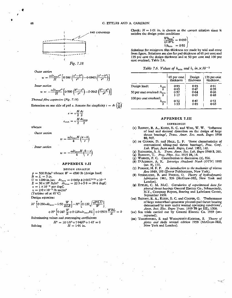
PAD EXPANDED

------- ----

--- 7 ------.-------- - -1 .

Fig. 7.18

Outer section adt,„„r2 (x2 1,2) (x5 --3.b311

w = [0 500 0 0943 H r. r /.1

Inner section

z o - aLjt IL2 [0.500 (b2 -2 x2)

0 0943 (b3 r-3 x3 )1 H r

Thermal fibre expansion (Fig. 7.18)

Extension on one side of pad e. Assume for simplicity t = dt (Pi)

H dt e - a 2 y

H dtmctx emax = a 2 2

whence

Outer section

nB2LU1 H4 [0•250adt,a, -1.50 -1/3 [0.1224/ ) W J

+H2 [ BLE

0.247 -w+0•128adtma,,BL1 +0.0503 WBL

Substituting values and rearranging coefficients H4 = 10.1113+7.94H2+1.47 =

Solving H = 1.01 in.

Inner section

w ad t„,a ,,H ix -1,1 4 kr/

adt„m „H 112- x\ w - 4 kr/

APPENDIX 7.11 DESIGN EXAMPLE

p = 500 lb/in2 whence W = 4500 lb (design load) B = L = 3 in. U = 1200 in./sec dtmax = 0.045p +2.00 U2'75 X10-8 E = 30 x 105 lb/in2 dtmax = 22.5+5.9 = 284 degC a = 1 X10-5 per degC

= 2.0 X 10-6 lb sec/in2 (Turbine oil at 85°C) Design equation:


Check: H = 1.01 in. is chosen as the correct solution since it satisfies the design point conditions

Whnil"2 - o 050 nU1321, 8/h„,i„ = 0.50

Solutions for minimum film thickness are made by trial and error from figure. Solutions are also for pad thickness of 65 per cent and 135 per cent the design thickness and at 50 per cent and 100 per cent overload, Table 7.6.

Table 7.6. Values of hinin and 8, in. X /0-3


Design thickness


Design load: h,„",1 0.93 0.93 0.91 S 0.83 047 0.35

50 per cent overload: h,„1„ 0.57 0.64 0.66 3 1.17 0.65 0.48

100 per cent overload: h,,,h, 0.32 0.47 0.51

S F53 0.85 0.63

APPENDIX 7.111 REFERENCES

(I) BAUDRY, R. A., KUHN, E. C. and WISE, W. W. 'Influence of load and thermal distortion on the design of large thrust bearings', Trans. Amer. Soc. mech. Engrs 1958 80, 807.

(2) DE GUERIN, D. and HALL, L. F. 'Some characteristics of conventional tilting-pad thrust bearings', Proc. Conf. Lub. Wear, Instn mech. Engrs, Lond. 1957, 142.

(3) RAIMONDI, A. A. Trans. Amer. Soc. Lub. Engrs 1960 3, 265. (4) BARRATT, T. Proc. Phys. Soc. 1915 28, 14. (5) WARNER, P. C. Contribution to discussion (i), 816. (6) D'Ammov, A. K. Izvestiga Akadernii Nauk (OTN) 1955

(no. 9), 170. (7) PURDAY, H. F. P. An introduction to the mechanics of viscous

flow 1949, 185 (Dover Publications, New York). (8) STERNLICHT, B. and Przlxus, 0. Theory of hydrodynamic

lubrication 1961, 326 (McGraw-Hill, New York and London).

(9) ETTLES, C. M. McC. Correlation of experimental data for pivoted thrust bearings General Electric Co., Schenectady, N.Y., Company Report, Bearing and Lubricant Centre, September 1959.

(Jo) BAUDRY, R. A., KUHN, E. C. and COOPER, G. 'Performance of large waterwheel-generator pivoted-pad thrust bearing determined by tests under normal operating conditions', Amer. Inst. Elec. Engrs Trans. 1959 78 (pt III), 1300.

- 0 (ii) Sea trials carried out by General Electric Co. 1959 (un- reported).

(12) TIMOSHENKO, S. and WOINOWSKY-KRIEGER, S. Theory of plates and shells second edition 1959 (McGraw-Hill, New York and London).

hydrodynamic thrust bearing study

Documents

Transcript of hydrodynamic thrust bearing study