Kinetic structure of rotational discontinuities: Implications for the magnetopause
The Pennsylvania State University
The Graduate School
Graduate Program in Acoustics
REFLECTION, RADIATION, AND COUPLING OF HIGHER
ORDER MODES AT DISCONTINUITIES IN FINITE LENGTH
RIGID WALLED RECTANGULAR DUCTS
A Thesis in
Acoustics
by
Ralph T. Muehleisen
c© 1996 Ralph T. Muehleisen
Submitted in Partial Fulfillmentof the Requirements
for the Degree of
Doctor of Philosophy
May 1996

We approve the thesis of Ralph T. Muehleisen.
Date of Signature
David C. SwansonAssistant Professor of AcousticsResearch AssociateThesis AdviserChair of Committee
Jiri TichyProfessor of AcousticsChairman of the Graduate Program in Acoustics
Scott D. SommerfeldtAssistant Professor of AcousticsResearch Associate
Douglas WernerResearch Associate

iii
Abstract
The effects of discontinuities on higher order modes is important in the design
of passive and active noise control systems in ducts which operate near or above the
cut-off frequency of the duct. Accurate acoustic monitoring of mechanical systems in
ducts at frequencies near and above the cut-off frequency of the first mode must include
the effects of discontinuities.
This thesis examines the reflection, transmission, and coupling of higher order
modes at discontinuities in finite length rigid walled rectangular ducts. Using a method of
generalized scattering coefficients, analytic expressions for the reflection and transmission
of higher order modes at size discontinuities, junctions, and baffled terminations are
developed. A technique to measure the higher order modes is discussed and implemented.
When written in matrix form, the equations for the reflection and transmission
coefficients for all three discontinuities take on the standard form for reflection and
transmission of plane waves at a change of impedance. For all the examples given, the
magnitude of the mutual coupling coefficients can be significant, often larger than that
of the self reflection and transmission coefficients, showing that modal coupling must be
included when working with models near and above the cut-off frequency of the first
higher order mode.
Analytic expressions for the reflection and transmission coefficients of a general
multi-port junction are derived in terms of the Green’s function of the junction region.
Examples of a right angle bend and a T junction are given. It is shown that the magnitude

iv
of the self transmission coefficient for the plane wave mode in the side branch to the end
of a T junction is found to have many zeros and the overall magnitude decreases with
increasing frequency indicating that side mounted speakers are poor plane wave sources
at frequencies near and above the cut-off of the first mode.
Analytic expressions for the radiation impedances and reflection coefficients for
the termination of a duct in an infinite baffle are derived. It is shown that the radiation
directivity is proportional to the wavenumber transform of the modal velocity. The plane
wave mode radiates omni-directionally at low frequencies and begins beaming on axis
at higher frequencies. The higher order modes radiate toward the sides, with the main
lobes moving toward the axis at higher frequencies. Equations for the total radiated
power in terms of the reflection coefficients of the duct termination and the incident
modal amplitudes are developed.
Experimental measurements of the reflection coefficients of an infinite baffle are
shown to be consistent with theory. Experimental measurements of the reflection and
transmission coefficients of a right angle bend are shown to be consistent with the junc-
tion theory. The thesis also gives a description of some of the potential problems involved
with modal measurement and microphone calibration.

v
Table of Contents
List of Figures . . . . . . . . . . . . . . . . . . . . . . . . . . . . . . . . . . . . . viii
List of Symbols . . . . . . . . . . . . . . . . . . . . . . . . . . . . . . . . . . . . . xv
Acknowledgments . . . . . . . . . . . . . . . . . . . . . . . . . . . . . . . . . . . xix
Chapter 1. Introduction . . . . . . . . . . . . . . . . . . . . . . . . . . . . . . . . 1
1.1 Historical Background . . . . . . . . . . . . . . . . . . . . . . . . . . 1
1.1.1 Early Work on Reflection and Radiation From Finite Ducts . 1
1.1.2 Early work on other Duct Discontinuities . . . . . . . . . . . 2
1.2 Motivation for Research and Thesis Goals . . . . . . . . . . . . . . . 5
1.3 Thesis Outline . . . . . . . . . . . . . . . . . . . . . . . . . . . . . . 6
Chapter 2. Math and Physics Review . . . . . . . . . . . . . . . . . . . . . . . . 8
2.1 Modal Decomposition . . . . . . . . . . . . . . . . . . . . . . . . . . 8
2.2 Matrix Notation . . . . . . . . . . . . . . . . . . . . . . . . . . . . . 13
2.3 Generalized Scattering Parameters . . . . . . . . . . . . . . . . . . . 14
2.4 Edge Condition . . . . . . . . . . . . . . . . . . . . . . . . . . . . . . 16
2.5 Green’s Functions . . . . . . . . . . . . . . . . . . . . . . . . . . . . . 17
Chapter 3. Modal Scattering at Step Discontinuities . . . . . . . . . . . . . . . 20
3.1 General Step Discontinuity Theory . . . . . . . . . . . . . . . . . . . 20
3.2 Numerical Considerations . . . . . . . . . . . . . . . . . . . . . . . . 25
vi
3.3 Coupling Matrix HRM for a Rectangular Duct . . . . . . . . . . . . 27
3.4 Examples . . . . . . . . . . . . . . . . . . . . . . . . . . . . . . . . . 29
3.4.1 An Asymmetric Stepped Duct . . . . . . . . . . . . . . . . . . 29
3.4.2 The Symmetric Stepped Duct . . . . . . . . . . . . . . . . . 47
Chapter 4. Modal Scattering at Junctions . . . . . . . . . . . . . . . . . . . . . 59
4.1 General Junction Theory . . . . . . . . . . . . . . . . . . . . . . . . . 59
4.2 Examples . . . . . . . . . . . . . . . . . . . . . . . . . . . . . . . . . 63
4.2.1 A Right Angle Bend . . . . . . . . . . . . . . . . . . . . . . . 64
4.2.2 A T Junction . . . . . . . . . . . . . . . . . . . . . . . . . . . 76
Chapter 5. Modal Scattering and Radiation at an Infinite Baffle . . . . . . . . . 97
5.1 General Derivation of Radiation Impedance . . . . . . . . . . . . . . 97
5.2 Development of Matrix Equations . . . . . . . . . . . . . . . . . . . . 101
5.3 ZrRM for a Rectangular Duct . . . . . . . . . . . . . . . . . . . . . . 102
5.4 Reflection Coefficients . . . . . . . . . . . . . . . . . . . . . . . . . . 108
5.5 Radiation . . . . . . . . . . . . . . . . . . . . . . . . . . . . . . . . . 114
5.5.1 Directivity . . . . . . . . . . . . . . . . . . . . . . . . . . . . . 114
5.5.2 Radiated Power . . . . . . . . . . . . . . . . . . . . . . . . . . 120
Chapter 6. Experimental Results . . . . . . . . . . . . . . . . . . . . . . . . . . 121
6.1 Modal Decomposition . . . . . . . . . . . . . . . . . . . . . . . . . . 121
6.1.1 Probes vs. Arrays . . . . . . . . . . . . . . . . . . . . . . . . 124
6.1.2 Horizontal vs. Axial Arrays . . . . . . . . . . . . . . . . . . . 125

vii
6.2 Modal Generation . . . . . . . . . . . . . . . . . . . . . . . . . . . . 126
6.3 Experimental Apparatus . . . . . . . . . . . . . . . . . . . . . . . . . 127
6.4 Data Reduction . . . . . . . . . . . . . . . . . . . . . . . . . . . . . . 131
6.5 Microphone Calibration and Measurement Caveats . . . . . . . . . . 131
6.6 Measurement of Reflection at an Infinite Baffle . . . . . . . . . . . . 133
Chapter 7. Conclusions and Suggestions For Future Research . . . . . . . . . . . 139
7.1 Conclusions . . . . . . . . . . . . . . . . . . . . . . . . . . . . . . . . 139
7.2 Suggestions for Future Research . . . . . . . . . . . . . . . . . . . . . 142
Appendix A. Infinite Summations Using Digamma Functions . . . . . . . . . . . . 145
Appendix B. Alternate Representation of ZrRM . . . . . . . . . . . . . . . . . . . 148
B.1 Conversion to a Convolution Integral . . . . . . . . . . . . . . . . . . 148
B.2 Review of Wavenumber Transforms . . . . . . . . . . . . . . . . . . . 149
B.3 Transformation of ZrRM . . . . . . . . . . . . . . . . . . . . . . . . . 151
B.4 Application to a Rectangular Duct . . . . . . . . . . . . . . . . . . . 152
Appendix C. Numerical Integration of ζRM . . . . . . . . . . . . . . . . . . . . . . 154
References . . . . . . . . . . . . . . . . . . . . . . . . . . . . . . . . . . . . . . . . 158
viii
List of Figures
2.1 A general N port junction . . . . . . . . . . . . . . . . . . . . . . . . . . 15
3.1 Geometry of the Stepped Duct in Example 3.4.1. . . . . . . . . . . . . . 21
3.2 Geometry of a General Rectangular Stepped Duct . . . . . . . . . . . . 27
3.3 Geometry of the Asymmetric Stepped Duct in Example 3.4.1. . . . . . . 30
3.4 Magnitude of the pressure self reflection coefficients in region 1, S11mm, for
incident modes m = 0, 1, 2, with a1/a2 = 2 and ε = 0. . . . . . . . . . . 35
3.5 Phase of the pressure self reflection coefficients in region 1, S11mm, for
incident modes m = 0, 1, 2, with a1/a2 = 2 and ε = 0. . . . . . . . . . . 36
3.6 Magnitude of the pressure self reflection coefficients in region 2, S22mm, for
incident modes m = 0, 1, 2, with a1/a2 = 2 and ε = 0. . . . . . . . . . . 37
3.7 Phase of the pressure self reflection coefficients in region 2, S22mm, for
incident modes m = 0, 1, 2, with a1/a2 = 2 and ε = 0. . . . . . . . . . . 38
3.8 Magnitude of the pressure self transmission coefficient of region 1 to
region 2, S21mm, for incident modes m = 0, 1, 2, with a1/a2 = 2 and ε = 0. 39
3.9 Magnitude of the pressure self transmission coefficient of region 2 to
region 1, S12mm, for incident modes m = 0, 1, 2, with a1/a2 = 2 and ε = 0. 40
3.10 Magnitude of the pressure mutual reflection and transmission coefficients
for incident mode 0 in region ν to mode 1 in region µ, Sµν10 , with a1/a2 = 2
and ε = 0. . . . . . . . . . . . . . . . . . . . . . . . . . . . . . . . . . . . 41
ix
3.11 Magnitude of the pressure mutual reflection and transmission coefficients
for incident mode 1 in region ν to mode 0 in region µ, Sµν01 , with a1/a2 = 2
and ε = 0. . . . . . . . . . . . . . . . . . . . . . . . . . . . . . . . . . . . 42
3.12 Magnitude of the pressure mutual reflection and transmission coefficients
for incident mode 0 in region ν to mode 2 in region µ, Sµν20 , with a1/a2 = 2
and ε = 0. . . . . . . . . . . . . . . . . . . . . . . . . . . . . . . . . . . . 43
3.13 Magnitude of the pressure mutual reflection and transmission coefficients
for incident mode 2 in region ν to mode 0 in region µ, Sµν02 , with a1/a2 = 2
and ε = 0. . . . . . . . . . . . . . . . . . . . . . . . . . . . . . . . . . . . 44
3.14 Magnitude of the pressure mutual reflection and transmission coefficients
for incident mode 1 in region ν to mode 2 in region µ, Sµν21 , with a1/a2 = 2
and ε = 0. . . . . . . . . . . . . . . . . . . . . . . . . . . . . . . . . . . . 45
3.15 Magnitude of the mutual pressure reflection and transmission coefficients
for incident mode 2 in region ν to mode 1 in region µ, Sµν12 , with a1/a2 = 2
and ε = 0. . . . . . . . . . . . . . . . . . . . . . . . . . . . . . . . . . . . 46
3.16 Geometry of the Symmetric Stepped Duct in Example 3.4.2. . . . . . . 47
3.17 Magnitude of the pressure self reflection coefficients in region 1, S11mm, for
incident modes m = 0, 1, 2 with a1/a2 = 2 and ε = (a1 − a2)/4. . . . . . 51
3.18 Phase of the pressure self reflection coefficients in region 1, S11mm, for
incident modes m = 0, 1, 2 with a1/a2 = 2 and ε = (a1 − a2)/4. . . . . . 52
3.19 Magnitude of the pressure self reflection coefficients in region 2, S22mm, for
incident modes m = 0, 1, 2 with a1/a2 = 2 and ε = (a1 − a2)/4. . . . . . 53

x
3.20 Phase of the pressure self reflection coefficients in region 2, S22mm, for
incident modes m = 0, 1, 2 with a1/a2 = 2 and ε = (a1 − a2)/4. . . . . . 54
3.21 Magnitude of the pressure self transmission coefficient of region 1 to
region 2, S21mm, for incident modes m = 0, 1, 2, with a1/a2 = 2 and
ε = (a1 − a2)/4. . . . . . . . . . . . . . . . . . . . . . . . . . . . . . . . . 55
3.22 Magnitude of the pressure self transmission coefficient of region 2 to
region 1, S12mm, for incident modes m = 0, 1, 2, with a1/a2 = 2 and
ε = (a1 − a2)/4. . . . . . . . . . . . . . . . . . . . . . . . . . . . . . . . . 56
3.23 Magnitude of the pressure mutual reflection and transmission coefficients
for incident mode 0 in region ν to mode 2 in region µ, Sµν20 , with a1/a2 = 2
and ε = (a1 − a2)/4. . . . . . . . . . . . . . . . . . . . . . . . . . . . . . 57
3.24 Magnitude of the pressure mutual reflection and transmission coefficients
for incident mode 2 in region ν to mode 0 in region µ, Sµν02 , with a1/a2 = 2
and ε = (a1 − a2)/4. . . . . . . . . . . . . . . . . . . . . . . . . . . . . . 58
4.1 Geometry of a Multi-port Junction . . . . . . . . . . . . . . . . . . . . . 60
4.2 Geometry of a Right Angle Duct Bend . . . . . . . . . . . . . . . . . . . 64
4.3 Magnitude of the pressure reflection coefficients of a right angle bend,
Rm0, for incident mode 0, into reflected modes m = 0, 1, 2. . . . . . . . . 70
4.4 Magnitude of the pressure reflection coefficients of a right angle bend,
Rm1, for incident mode 1, into reflected modes m = 0, 1, 2. . . . . . . . . 71
4.5 Magnitude of the pressure reflection coefficients of a right angle bend,
Rm2, for incident mode 2, into reflected modes m = 0, 1, 2. . . . . . . . . 72
xi
4.6 Magnitude of the pressure transmission coefficients of a right angle bend,
Tm0, for incident mode 0, into transmitted modes m = 0, 1, 2. . . . . . . 73
4.7 Magnitude of the pressure transmission coefficients of a right angle bend,
Tm1, for incident mode 1, into transmitted modes m = 0, 1, 2. . . . . . . 74
4.8 Magnitude of the pressure transmission coefficients of a right angle bend,
Tm2, for incident mode 2, into transmitted modes m = 0, 1, 2. . . . . . . 75
4.9 Geometry of a T Junction . . . . . . . . . . . . . . . . . . . . . . . . . . 76
4.10 Magnitude of the pressure reflection coefficients of one end of a T junc-
tion, S11m0, for incident mode 0 into reflected modes m = 0, 1, 2. . . . . . 82
4.11 Magnitude of the pressure reflection coefficients of the side branch of a
T junction, S22m0, for incident mode 0 into reflected modes m = 0, 1, 2. . 83
4.12 Magnitude of the pressure transmission coefficients S21m0, from mode 0 in
one end of a T to modes m = 0, 1, 2 in the side branch. . . . . . . . . . . 84
4.13 Magnitude of the pressure transmission coefficients S12m0, from mode 0 in
the side branch of a T to modes m = 0, 1, 2 in one end. . . . . . . . . . . 85
4.14 Magnitude of the pressure transmission coefficients S13m0, from mode 0 in
one end of a T to modes m = 0, 1, 2 in the other end. . . . . . . . . . . . 86
4.15 Magnitude of the pressure reflection coefficients S11m1, end of a T junction
for incident mode 1 into reflected modes m = 0, 1, 2. . . . . . . . . . . . 87
4.16 Magnitude of the pressure reflection coefficients S22m1, from the side branch
of a T junction for incident mode 1 into reflected modes m = 0, 1, 2. . . 88
4.17 Magnitude of the pressure transmission coefficients S21m1, from mode 1 in
one end of a T to modes m = 0, 1, 2 in the side branch. . . . . . . . . . . 89
xii
4.18 Magnitude of the pressure transmission coefficients S12m1, from mode 1 in
the side branch of a T to modes m = 0, 1, 2 in one end. . . . . . . . . . . 90
4.19 Magnitude of the pressure transmission coefficients S13m1, from mode 1 in
one end of a T to modes m = 0, 1, 2 in the other end. . . . . . . . . . . . 91
4.20 Magnitude of the pressure reflection coefficients, S11m2, from of one end of
a T junction for incident mode 2 into reflected modes m = 0, 1, 2. . . . . 92
4.21 Magnitude of the pressure reflection coefficients S22m2. . . . . . . . . . . . 93
4.22 Magnitude of the pressure transmission coefficients S21m2, from mode 2 in
one end of a T to modes m = 0, 1, 2 in the side branch. . . . . . . . . . . 94
4.23 Magnitude of the pressure transmission coefficients S12m2, from mode 2 in
the side branch of a T to modes m = 0, 1, 2 in one end. . . . . . . . . . . 95
4.24 Magnitude of the pressure transmission coefficients S13m2, from mode 2 in
one end of a T to modes m = 0, 1, 2 in the other end. . . . . . . . . . . . 96
5.1 Geometry used in calculating reflection and radiation from a baffled duct. 98
5.2 Normalized self radiation resistances of an infinite baffle, Re{ζmm}, for
m = 0, 1, 2, with a/b = 2.25 . . . . . . . . . . . . . . . . . . . . . . . . . 104
5.3 Normalized self radiation reactances of an infinite baffle, Im{ζmm}, for
m = 0, 1, 2 with a/b = 2.25. . . . . . . . . . . . . . . . . . . . . . . . . . 105
5.4 Normalized mutual radiation resistances of an infinite baffle, Re{ζrm}
and Im{ζrm}, for m = 0, 1, 2 with a/b = 2.25. . . . . . . . . . . . . . . . 106
5.5 Normalized mutual radiation reactances of an infinite baffle, Re{ζrm}
and Im{ζrm}, for m = 0, 1, 2 with a/b = 2.25. . . . . . . . . . . . . . . . 107

xiii
5.6 Magnitude of the self pressure reflection coefficients of an infinite baffle,
Rmm, for m = 0, 1, 2 with a/b = 2.25. . . . . . . . . . . . . . . . . . . . . 110
5.7 Phase of the self pressure reflection coefficients of an infinite baffle, Rmm,
for m = 0, 1, 2 with a/b = 2.25. . . . . . . . . . . . . . . . . . . . . . . . 111
5.8 Magnitude of the mutual pressure reflection coefficients R02 and R20 of
an infinite baffle for m = 0, 1, 2, with a/b = 2.25. |R00| is shown for
comparison. . . . . . . . . . . . . . . . . . . . . . . . . . . . . . . . . . . 112
5.9 Phase of the mutual reflection coefficients R02 and R20 of an infinite
baffle for m = 0, 1, 2, with a/b = 2.25. The phase of R00 is shown for
comparison. . . . . . . . . . . . . . . . . . . . . . . . . . . . . . . . . . . 113
5.10 D00(φ), the directivity of the radiated pressure for a plane wave mode
incident at an infinite baffled end with θ = 0 and a/b = 2.25 . . . . . . . 117
5.11 D10(φ), the directivity of the radiated pressure for the first horizontal
mode incident at an infinite baffled end θ = 0 and a/b = 2.25 . . . . . . 118
5.12 D20(φ), the directivity of the radiated pressure for the second horizontal
mode wave mode incident at an infinite baffled end with θ = 0 and
a/b = 2.25 . . . . . . . . . . . . . . . . . . . . . . . . . . . . . . . . . . . 119
6.1 Side mounted speaker configuration . . . . . . . . . . . . . . . . . . . . . 126
6.2 Back mounted speaker configuration . . . . . . . . . . . . . . . . . . . . 127
6.3 Duct Setup . . . . . . . . . . . . . . . . . . . . . . . . . . . . . . . . . . 128
6.4 Microphone Array Setup . . . . . . . . . . . . . . . . . . . . . . . . . . . 129
6.5 Overall Experimental Setup . . . . . . . . . . . . . . . . . . . . . . . . . 130
xiv
6.6 Baffle Used for Reflection Coefficient Measurements. . . . . . . . . . . . 134
6.7 Comparison of theoretical and experimentally determined magnitude of
the plane wave mode self pressure reflection coefficient R00. . . . . . . . 136
6.8 Comparison of theoretical and experimentally determined magnitude of
the first mode self pressure reflection coefficient R11. . . . . . . . . . . . 137
6.9 Comparison of theoretical and experimentally determined mutual pres-
sure reflection coefficient magnitude R20. . . . . . . . . . . . . . . . . . . 138
C.1 integration of the rectangular region . . . . . . . . . . . . . . . . . . . . 156
xv
List of Symbols
AM , BM modal amplitudes of mode M
A, B modal amplitude vectors
CM total amplitude of mode M
DM (φ, θ) radiation directivity function of mode M
G(~x| ~x0) Green’s function
G generalized inverse of H
HRM step discontinuity coupling constant from mode M to mode R
H step discontinuity coupling constant matrix
KM eigenvalue for mode M of an enclosure
Lx, Ly, Lz duct dimensions
M,N,R, S mode number pairs or triplets
PM modal pressure amplitude
PM modal pressure amplitude matrix
PMZ modal pressure amplitude matrix, alternate form
R(x, y, z) position vector
RMN reflection coefficient from mode N to mode M
R reflection matrix
SliRM scattering parameter between mode M in duct i and mode R in duct l
Sli scattering matrix from duct i to duct l
TMN transmission coefficient from mode N to mode M

xvi
T transmission matrix
YM specific acoustic modal admittance of mode M
Y specific acoustic modal admittance matrix
Zc specific acoustic modal impedance matrix
ZRM mutual modal impedance between modes M and R
Z mutual modal impedance matrix
ZrRM mutual modal radiation impedance between modes M and R
Zr mutual modal radiation impedance matrix
Nsubscript number of modes in region subscript
Ssubscript area of region subscript
a, b, c, d duct dimensions
c ambient speed of sound in air
j√−1
k acoustic wavenumber
mx, nx, rx, sx mode numbers in the x direction
my, ny, ry, sy mode numbers in the y direction
mz, nz, rz , sz mode numbers in the y direction
~n surface normal vector
p′(x, y, z, t) linear acoustic pressure perturbation
p(x, y, z, ω) Fourier transform of the linear acoustic pressure perturbation
p pressure amplitude matrix
pM pressure amplitude of mode M
xvii
r(x, y, z) position vector
t time
u′(x, y, z, t) linear acoustic velocity perturbation
u(x, y, z, ω) Fourier transform of the linear acoustic velocity perturbation
x, y, z Cartesian coordinates
x0, y0, z0 source location in Cartesian coordinates
ΠM power in mode M
Π+,Π− total incident and reflected power
ΠRad total radiated power
PsiM (kx, ky) spatial Fourier transform of psiM(x, y)
χM eigenvalue of ΨM
Λmx ,Λmy integration constant
δmn Kronecker delta function
δ~x Dirac delta function at position ~x
ηRM normalized mutual modal impedance from mode M to mode R
η normalized mutual modal impedance matrix
α, β polar transformation variables
γM propagation constant for mode M
ψM (x, y) eigenfunction (mode shape) of mode M
ρ ambient density of air
ω radian frequency
φ polar angle in x, z plane
xviii
φ+, φ− propagation matrices
θ polar angle from z axis
ζRM normalized mutual modal radiation impedance from mode M to mode R
ζ normalized mutual modal radiation impedance matrix
∇ gradient operator
∇2 Laplacian operator
matrixH matrix hermitian operator
={q} imaginary part of the complex argument q
<{q} real part of the complex argument q
matrixT matrix transpose operator
xix
Acknowledgments
I would like to thank “The man of a thousand and one ideas”, my advisor, David
Swanson. His patience, encouragement, guidance and financial support were essential to
the completion of this thesis.
I would like to thank my other thesis committee members for their suggestions
and criticism, and especially Doug Werner for his willingness to serve on such short
notice.
I thank the other members of Dave Swanson’s research group, especially Karl
Reichard and Mark Mahon for their overall help in the completion of this thesis.
I want to thank the Applied Research Lab and Dr. Richard Stern for early
financial support through the Exploratory and Foundational Research program.
I would like to thank all the wonderful instructors here at Penn State, but in
particular I’d like to thank Courtney Burroughs, Gary Koopman, Allan Pierce (despite
the 8am classes), Victor Sparrow, Scott Sommerfeldt, Jiri Tichy and William Thompson
Jr. for always keeping me thinking and for always being willing to answer even the most
stupid questions.
I would like to thank Brian Bourgault of Mathworks for providing a free beta
copy of MATLAB for Linux which was used for most of the numerical analysis in the
thesis.

xx
Big thanks go to the greatest set of administrative assistants at Penn State,
Karen Brooks, Catherine Brown, Barbara Crocken, and Carolyn Smith for all their
help throughout the years.
I would like to thank all my fellow students and friends in the Graduate Program
in Acoustics for all their support, witty banter, mindless diversions and willingness to
help me whenever I needed it, especially Ben Bard, Scott Hansen, Mary Herr, Brian
Katz, Doug Koehn, Rod Korte, Tim Leishmann, Andy Mills, Judy Rochat, Tad Rollow,
Dan Russell, and Brian Scott. In particular, I’d like to thank Ed “Reverse the Drill”
Maniet and Paul “Carriage Bolts” Moran who helped keep me sane during the last
few months of work. I wish everyone could have office-mates as great as you two. I
would like thank a few former students and other friends who have given me guidance
and encouragement: Paul Kovitz, Rob and Tammie Lepage (and the uncountable clan),
Russ McMillan, Martin Manley, Doug Mast and Andy Piascek.
I would like to thank my parents, my brother, my Brother-in-law Jerome and my
sister Vicky for their encouragement. I especially thank Vicky for letting me finish first.
Most of all I have to thank my dear wife Sally Laurent-Muehleisen. Without her
love, encouragement, guidance, patience and example, this thesis could never have been
written. This thesis is dedicated to her, with love until love has no meaning.
1
Chapter 1
Introduction
1.1 Historical Background
1.1.1 Early Work on Reflection and Radiation From Finite Ducts
Research on acoustic waveguides dates back at least as far as Lord Rayleigh
[52]. Rayleigh determined the eigenfunctions of infinitely long rigid walled rectangular
and circular waveguides. Rayleigh also analytically determined end corrections (from
which reflection coefficients can be determined) for low frequency radiation from a baffled
circular duct. The analysis was limited to frequencies far below the cut-off frequency of
the first higher order mode. Rayleigh did not determine end corrections for rectangular
ducts. Rayleigh was unable to determine analytic expressions for end corrections to an
unbaffled circular duct, but he did determine empirical expressions.
Analysis of the unbaffled circular duct proved most troublesome. It was not until
Levine and Schwinger [32] employed the Weiner-Hopf technique that analytic expressions
of the reflection coefficients for an unbaffled circular duct were obtained. However, their
analysis was still limited to frequencies below the cut-off frequency of the first higher
order mode. This analysis was refined by several authors [42, 47].
Weinstein [68], also employing Weiner-Hopf methods, was able to determine re-
flection coefficients for higher order modes at the end of an unbaffled circular duct. In
addition, Weinstein obtained analytic expressions for the reflection coefficients from the
2
end of plane parallel waveguides (two semi-infinite parallel plates). Weinstein found that
for an incident plane wave above the cut-off frequency of the first higher order mode, the
magnitude of the mutual reflection coefficient between the plane wave mode and the first
higher order mode can be significantly greater than the magnitude of the plane wave self
reflection coefficient. This result showed that coupling between modes at the end of a
duct is very important when analyzing wave propagation at higher frequencies.
Unfortunately, the Weiner-Hopf method does not allow one to determine the
radiation from the end of rectangular ducts [68]. Even if it did, the mathematics of the
Wiener-Hopf method is steeped in the concepts of analytic function theory and is very
involved. The results are often difficult to numerically evaluate and meaningful physical
interpretation of the results can get lost in the myriad of mathematical symbols.
Zorumski [70] developed the concept of generalized radiation impedances and re-
flection coefficients for infinitely baffled circular ducts. He developed matrix formulations
for the generalized impedance. The method of analysis used in this thesis is similar to
the method Zorumski used.
Recently there has been a large number of papers about radiation from baffled
and unbaffled circular ducts [22, 37, 48, 67]. Much of the work has been prompted by
research in the acoustics of turbofan and turbojet engines.
1.1.2 Early work on other Duct Discontinuities
The low frequency lumped element analysis of acoustic duct discontinuities such
as constrictions, bifurcations, and size changes dates back to Rayleigh as well, but an
early thorough analysis dates back to Mason’s work [36] on acoustical filters.
3
Miles [38, 39, 40] extended this work to be valid at frequencies much closer to the
cut-off frequency of the first higher order mode. He basically used a truncated version of
the mode matching technique that Mittra and Lee were to later use in electromagnetic
problems. The thrust of Miles’ research was to develop more accurate lumped element
equivalents of discontinuities.
Soon after Miles’ papers appeared, Lippert [33, 34] published his research on
modal measurement techniques along with theory and experiments on right angled bends.
Doak’s excellent set of papers [18, 19] which discusses higher order modes in rigid
walled rectangular ducts, was a thorough analysis of the generation and propagation of
higher order modes. However Doak’s analysis did not give a good description of the
coupling of higher order modes, an effect which is important at any discontinuity when
higher order modes can propagate. This paper was an important basis for the analysis
of ducting systems and mufflers at higher frequencies. It also rekindled interest in higher
order mode research.
Following Doak’s work, a number of other papers looking at the propagation and
coupling of higher order modes for several different discontinuities in rectangular and
circular ducts were written.
Cummings [17] looked at propagation through 180 degree bends. Firth and Fahy
[21] and Furnell and Bies [23, 24] both looked at curved bends in ducts.
Said [58] looked at propagation in right angle bends and T junctions. He derived
and measured energy coupling coefficients instead of pressure coupling coefficients.
About this same time, the finite element technique began to be applied to acoustic
waveguide problems [14, 15]. While this powerful method allows one to determine the
4
overall propagation through a complicated system, it is difficult to determine quantities
like modal amplitudes and coupling coefficients using it. In addition, much of the physics
is lost because there are no analytic results, just tables of numbers.
Nevertheless, Shepherd and Cabelli [59, 60] looked at propagation through right
angled bends using finite elements. They compared their finite element results to exper-
imental results and showed a high degree of accuracy.
Redmore and Mulholland [54] looked at propagation past a side branch (a T
junction) using modal analysis. However, they didn’t explicitly derive reflection and
transmission coefficients, they simply predicted the pressure at a given point in the side
branch.
Working with electromagnetic waveguides, Mittra and Lee [41] developed mode
matching techniques which lend themselves to numerical solutions for problems in which
the Wiener-Hopf method does not apply. The idea of mode matching techniques at a
discontinuity is to expand the solution on either side of the discontinuity in an orthogonal
modal series. Using equations of continuity (in acoustics the pressure and normal velocity
are usually continuous) a number of simultaneous equations are developed. Through the
use of orthogonality the equations can be reduced and solved.
The development of planar microwave waveguide circuits has lead to great ad-
vances in scattering theory for microwave junctions using mode matching techniques
and generalized scattering parameters. [28, 49, 56]. In particular, MacPhie and Zaghloul
published a paper on radiation from a baffled rectangular waveguide [35]. However, the
electromagnetic waveguide is different enough from the acoustic waveguide that the work
done in microwave research cannot be applied directly to acoustic waveguides. Hudde
5
[26, 27] has recently begun applying the mode-matching and generalized scattering pa-
rameter techniques to acoustic waveguide problems; however, his work has been limited
to circular waveguides.
A need to examine propagation at higher frequencies has re-emerged with the
development of active noise control systems. Much analysis has been done assuming
plane wave propagations. A few researchers have investigated the effects of higher order
modes on active control [65], while others have looked at the effects of modal coupling on
plane wave propagation [45]. A number of initial investigations into higher order modal
control [3, 4, 55, 61, 62, 63, 64] have been made, but none have considered the modal
coupling present at discontinuities.
1.2 Motivation for Research and Thesis Goals
While there certainly has not been an absence of work in duct acoustics, there
has not been much done on the scattering and coupling of higher order acoustic modes,
especially for rectangular ducts.
The main goal of this thesis is to develop a coherent theory of scattering at modal
discontinuities. In particular, reflection and transmission coefficients will be determined
in terms of generalized scattering parameters and generalized impedances. A few of the
calculations will be experimentally verified.
The applications of such theory are numerous. An obvious application is in acous-
tical analysis of air flow and industrial HVAC systems with large cross sections. Such
systems often have higher order mode propagation in them. It is often impractical to add
enough damping to an air flow system for the desired acoustic noise reduction. Proper
6
design of acoustical filters would let the acoustical properties of the ducts themselves
reduce the propagated noise. Standard plane wave analysis is an insufficient tool for
higher frequency filter design. As active noise control (ANC) strives to make inroads
into industry, the bandwidth of such systems will have to be increased to control sound
above the cut-off frequency of the ducting system. Proper analysis of modal scattering
is essential in the design of an effective higher frequency ANC system. A less obvious
application is the acoustical monitoring of mechanical systems, where often the acous-
tical signal that is desired to be measured is a high frequency signal traveling though a
ducting system (e.g. turbofans, fluid piping systems). A knowledge of how the ducting
system modifies the acoustic spectrum is essential in acoustical monitoring.
1.3 Thesis Outline
Chapter 2 of the thesis reviews some of the mathematics and physics of duct
acoustics and modal analysis. In particular, the chapter discusses the equations governing
wave propagation in ducts and discusses their solution in modal form. It develops matrix
forms of those same solutions. It also reviews the use of generalized scattering parameters
and Green’s functions in the solution of acoustic waveguide problems.
Chapter 3 of the thesis derives the scattering parameters for step (size) discon-
tinuity. Examples of symmetric and asymmetric steps in a rectangular waveguide are
given.
Chapter 4 of the thesis derives the scattering parameters for multi-port junctions.
Right angle bends and T junctions in rectangular waveguides are used as examples. The
7
analytical results for the right angle bend are compared with the experimental results fo
Sheperd and Cabelli [59].
Chapter 5 of the thesis derives expressions for the radiation impedance and re-
flection coefficients for a duct terminating in an infinite baffle. Numerical results are
obtained for a rectangular waveguide. Expressions for the radiated power and directiv-
ity of the radiation from the duct termination are developed.
Chapter 6 of the thesis discusses the experimental methods used to investigate
radiation from the end of a baffled rectangular duct.
Chapter 7 states some conclusions which can be drawn from the work and gives
suggestions for future research.
8
Chapter 2
Math and Physics Review
This chapter of the thesis will briefly review some of the basic mathematics and
physics of duct acoustics and scattering parameters. In particular, it will cover modal
decomposition, the edge condition, scattering parameters, matrix notation and Green’s
functions.
2.1 Modal Decomposition
A linear fluid pressure perturbation p′(x, y, z) inside an acoustic waveguide satis-
fies the linear acoustic pressure wave equation
(∇2 − 1c2
∂
∂t2)p′(x, y, z, t) = 0 (2.1)
where t represents time and c represents the acoustic speed of sound in the medium. The
fluid pressure perturbation, p′, and the particle velocity perturbation, u′, are related by
the linearized momentum equation, also known as Euler’s equation
ρ∂~u′(x, y, z, t)
∂t= −∇p′(x, y, z, t) (2.2)
where ρ is the ambient density of the medium.
9
The linearized wave and Euler’s equation can be Fourier transformed in time to
yield the constant frequency versions of the equations.
The forward Fourier time transform is defined as
F (x, y, z, ω) =∞∫−∞
f(x, y, z, t)e−jwtdt. (2.3)
The inverse Fourier time transform is defined as
f(x, y, z, t) =1
2π
∞∫−∞
F (x, y, z, ω)ejwtdω. (2.4)
Denoting the Fourier Transform of the linear pressure perturbation p′ as p, the
Fourier transformed wave equation (also known as the Helmholtz equation) can be writ-
ten as
(∇2 + k2)p(x, y, z, ω) = 0 (2.5)
where the wavenumber k = ω/c.
Denoting the Fourier transform of the linear velocity perturbation ~u′ as ~u, the the
Fourier transformed form of Euler equation is
~u(x, y, z, ω) =j
kρc∇p(x, y, z, ω). (2.6)
The solution to the differential equation 2.5 depends upon the boundary condi-
tions. If the fluid is confined to a rectangular duct with rigid walls at x = 0, x = a,
10
y = 0, and y = b, the normal velocity is zero on each wall. The boundary conditions are
then
∂
∂xp∣∣∣x=0
=∂
∂xp∣∣∣x=a
=∂
∂yp∣∣∣y=0
=∂
∂yp∣∣∣y=b
= 0. (2.7)
The pressure can be expressed as an expansion of the eigenfunctions of the partial
differential equation. The eigenfunctions are called the modes of the system, and the
eigenfunction expansion is called the modal solution.
In the case of a duct constrained in the x and y direction the modal solution for
the pressure is
p(x, y, z) =∑mx
∑my
(Amxmye−γmxmy z +Bmxmye
γmxmy z)ψmxmy(x, y) (2.8)
where ψmxmy is the eigenfunction (also known as the duct mode) and the propagation
constant γmxmy =√χ2mxmy − k2 where χmxmy is the eigenvalue associated with ψmxmy .
Because the modes are the eigenfunctions of a self-adjoint differential equation,
they are real and orthogonal [31, 43, 69]. When the modes are properly normalized, the
orthogonality integral takes the form
∫∫S
ψmxmy(x, y)ψnxny(x, y)dS = δmxnxδmyny (2.9)

11
where S is the cross sectional area of the duct and δmn is the Kronecker delta defined by
δmn =
1 m = n
0 m 6= n
. (2.10)
The coefficients Amxmy and Bmxmy in equation 2.8 are called the modal ampli-
tudes. Amxmy is the amplitude of the waves traveling in the +z direction, while Bmxmy
is the amplitude of the waves traveling in the −z direction.
ψmxmy(x, y) are the modes of the duct. They represent standing waves that exist
in the x and y directions of the duct.
For each mx,my there is a frequency at which γmxmy is zero. That frequency is
called the cut-off frequency. Below the cut-off frequency the mode is called evanescent
because γmxmy is real and the mode no longer propagates, but decays exponentially.
The propagation constant γmxmy is used instead of the modal wavenumber kmxmy =√k2 − χ2
mxmy because using this notation ensures that evanescent waves are represented
with decaying amplitude. To ensure that evanescent modes are represented with decaying
amplitude, one must take the negative root of k2−χ2mxmy when k2 < χ2
mxmy , something
which is not easily implemented when solving the propagation equations numerically.
For a rectangular duct of sides a and b the normalized mode ψmxmy is given by
ψmx,my(x, y) =cos(mxπa x) cos(myπb y)√
abΛmxΛmy(2.11)
12
where the integration constant Λmx is given by
Λmx =
1 mx = 0
12 mx > 0
. (2.12)
For the same duct the propagation number is given by
γmxmy =√
(mxπ
a)2 + (
myπ
b)2 − k2. (2.13)
Because nearly all the summations in this thesis will be double or triple summa-
tions (for the x, y, and z modes), a new terminology will be used. Capital letters will be
used to denote summation pairs or triplets. For example, M refers to mxmy or mxmymz
and N to nxny or nxnynz.
With the new summation notation equations 2.8 through 2.13 become
p(x, y, z) =∑M
(AMe−γMz +BMeγM z)ψM (x, y) (2.14)
ψM (x, y) =cos(mxπa x) cos(myπb y)√
abΛmxΛmy(2.15)
and
γM =√
(mxπ
a)2 + (
myπ
b)2 − k2. (2.16)
The axial velocity, uz, in the duct can be determined using Euler’s equation.
Application of Euler’s equation to equation 2.14 yields
13
uz(x, y, z) =∑M
YM(AMe−γM z −BMeγM z)ψM (x, y) (2.17)
where the specific modal admittance YM is given by
YM =−jγMkρc
. (2.18)
The specific modal admittance is the ratio of the acoustic velocity to the acoustic
pressure for a particular mode propagating in one direction in an infinite duct.
2.2 Matrix Notation
Many of the modal summations can be more simply represented as matrix mul-
tiplications. With a more simple representation the physics of the problem should be
easier to see. In addition, the matrix representation is easily coded when using a higher
level language like MATLAB.
First, a number of vectors and matrices must be defined. Let
A =
A0
A1
...
B =
B0
B1
...
ψ =
ψ0(x, y)
ψ1(x, y)
...
Y =
Y0 0 · · ·
0 Y1 · · ·...
.... . .
(2.19)
φ− =
e−γ0z 0 · · ·
0 e−γ1z · · ·...
.... . .
φ+ =
eγ0z 0 · · ·
0 eγ1z · · ·...
.... . .
. (2.20)
14
With these definitions, and noting that T denotes the transpose operation, equa-
tion 2.14 can be rewritten
p(x, y, z) = ψT φ−A+ ψT φ+B (2.21)
and equation 2.17 can be rewritten
uz(x, y, z) = ψT Y φ−A− ψT Y φ+B. (2.22)
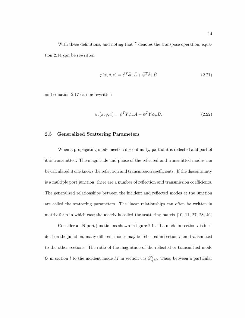
2.3 Generalized Scattering Parameters
When a propagating mode meets a discontinuity, part of it is reflected and part of
it is transmitted. The magnitude and phase of the reflected and transmitted modes can
be calculated if one knows the reflection and transmission coefficients. If the discontinuity
is a multiple port junction, there are a number of reflection and transmission coefficients.
The generalized relationships between the incident and reflected modes at the junction
are called the scattering parameters. The linear relationships can often be written in
matrix form in which case the matrix is called the scattering matrix [10, 11, 27, 28, 46]
Consider an N port junction as shown in figure 2.1 . If a mode in section i is inci-
dent on the junction, many different modes may be reflected in section i and transmitted
to the other sections. The ratio of the magnitude of the reflected or transmitted mode
Q in section l to the incident mode M in section i is SliQM . Thus, between a particular
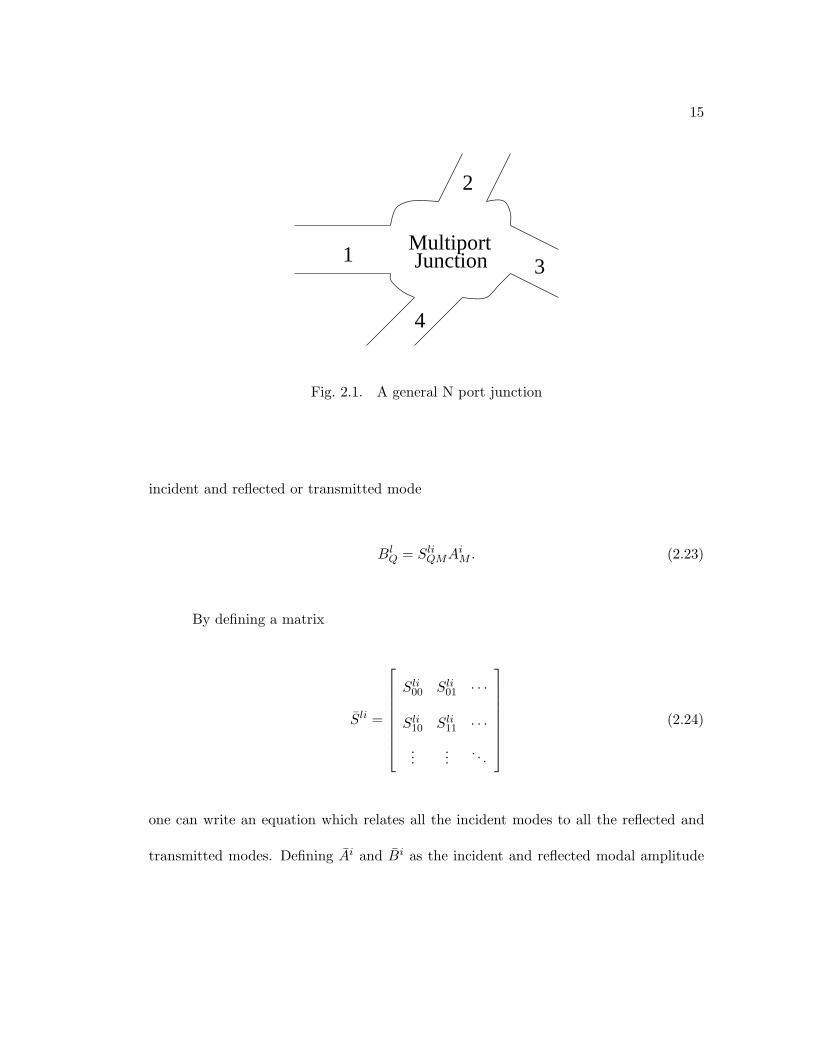
15
4
1
2
3JunctionMultiport
Fig. 2.1. A general N port junction
incident and reflected or transmitted mode
BlQ = SliQMA
iM . (2.23)
By defining a matrix
Sli =
Sli00 Sli01 · · ·
Sli10 Sli11 · · ·...
.... . .
(2.24)
one can write an equation which relates all the incident modes to all the reflected and
transmitted modes. Defining Ai and Bi as the incident and reflected modal amplitude
16
vectors in the ith section this equation is
B1
B2
...
BN
=
S11 S12 · · · S1N
S21 S22 · · · S2N
......
. . ....
SN1 SN2 · · · SNN
A1
A2
...
AN
. (2.25)
2.4 Edge Condition
When doing numerical computations using modal analysis, the infinite sums and
infinite dimension matrices developed earlier must be truncated to a finite size. When
working with modal expansions in two connected regions one must be very careful about
the number of modes which are used in each region. Early work with electromagnetic
waves showed a phenomenon known as relative convergence, whereby the solution con-
verges to different values depending upon how the modal decomposition was truncated.
By changing the ratio of number of modes in each region, different solutions were ob-
tained.
It has been found that relative convergence is related to the violation of energy
relations at the edge of a discontinuity [28, 41]. By imposing conservation of energy
at the boundary, specific ratios of the number of modes required in each region can
be developed. For regions of similar geometry (i.e circular to circular, rectangular to
rectangular) Mittra and Lee found that the ratio of number of modes was the same as
the ratio of the characteristic sizes. For example, when dealing with two circular ducts
with a radius ratio of 2:1 the number of modes must be 2:1.
17
2.5 Green’s Functions
Solving the wave equation with finite sized sources can sometimes be a daunting
task. One of the more powerful techniques for solving boundary value problems like those
posed by duct acoustics is the use of Green’s functions [2, 12, 13, 31, 43, 44, 50, 69]. The
use of Green’s functions will be essential for determining reflection and transmission at
junctions and reflection and radiation from the end of the duct.
A Green’s function G(~x| ~x0) for the Helmholtz equation satisfies the inhomoge-
neous differential equation
(∇2 + k2)G(~x| ~x0) = −δ(~x− ~x0). (2.26)
In acoustics, the Green’s function G(~x| ~x0) describes the propagation of radiation
from a point source at ~x0 to the point ~x. The pressure at ~x radiated from a vibrating
region of space S0 propagating through a region with a Green’s function G(~x| ~x0) can be
determined using the Kirchoff-Helmholtz integral theorem [30, 44, 50] which states
p(~x) = −∫∫S0
[G(~x| ~x0)∇p( ~x0)− p( ~x0)∇G(~x| ~x0)] · ~ndS0 (2.27)
where ~n is the surface normal and S0 is the radiating surface area.
For a point source in free space the Green’s function can be shown to be [44, 50]
G(~x| ~x0) =ejkr
4πr(2.28)
18
where r =√
(x− x0)2 + (y − y0)2 + (z − z0)2.
If the point source is above a rigid plane the particle velocity at the rigid plane
must be zero. A new Green’s function can be developed through the use of image sources
which satisfies this boundary condition. If the source is located on the rigid plane (not
just above) at z0 = 0 a suitable Green’s function is [44, 50]
G(~x| ~x0) =ejkr
2πr(2.29)
where r =√
(x− x0)2 + (y − y0)2 + z2.
This Green’s function has the property that ∇g(~x| ~x0) · z = 0 on the plane z = 0.
Thus when equation 2.29 is used, equation 2.27 reduces to
p(~x) = jkρc
∫∫S0
uz(S0)G(~x| ~x0)dS0. (2.30)
This equation is known as the Rayleigh Integral. It is an indispensable equation
for determining the radiation from a planar region in an infinite baffle.
If the source is inside an enclosure instead of in free space the Green’s function
can be found as an expansion of modes of the enclosure [44, 50]
G(~x| ~x0) =∑mx
∑my
∑mz
φmxmymz (~x)φmxmymz( ~x0)K2mxmymz − k2
=∑M
φM (~x)φM ( ~x0)K2M − k2
(2.31)
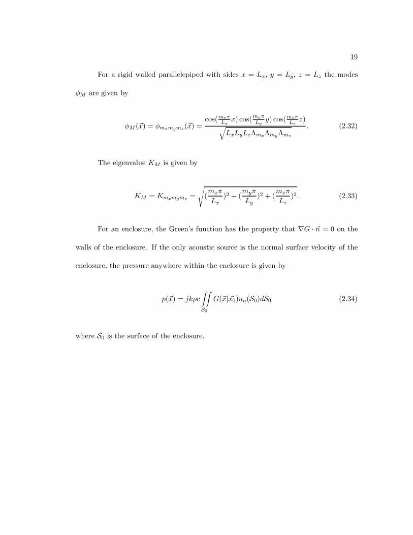
19
For a rigid walled parallelepiped with sides x = Lx, y = Ly, z = Lz the modes
φM are given by
φM (~x) = φmxmymz(~x) =cos(mxπLx
x) cos(myπLyy) cos(mzπLz z)√
LxLyLzΛmxΛmyΛmz. (2.32)
The eigenvalue KM is given by
KM = Kmxmymz =√
(mxπ
Lx)2 + (
myπ
Ly)2 + (
mzπ
Lz)2. (2.33)
For an enclosure, the Green’s function has the property that ∇G · ~n = 0 on the
walls of the enclosure. If the only acoustic source is the normal surface velocity of the
enclosure, the pressure anywhere within the enclosure is given by
p(~x) = jkρc
∫∫S0
G(~x| ~x0)un(S0)dS0 (2.34)
where S0 is the surface of the enclosure.

20
Chapter 3
Modal Scattering at Step Discontinuities
Two of the discontinuities present in many ducting systems are constrictions and
expansions - changes in the area of the duct. This is known in the microwave field as a
step discontinuity. Step discontinuities are essential parts of acoustical filter design.
This chapter of the thesis will present a thorough analysis of the reflection and
transmission of different modes at a step discontinuity. Using the formalism of general-
ized scattering parameters, both the constriction and expansion problems can be solved
at the same time.
3.1 General Step Discontinuity Theory
A general step discontinuity is shown in figure 3.1. Consider a change of size in
an infinite duct at z = 0. The main duct, in region 1, has a cross sectional area S1. The
smaller duct, in region 2, has a cross sectional area S1. The area at z = 0 of S1 outside
S2 will be denoted S3. In region 1 modes A1M are incident on the junction and B1
M are
traveling away from it. In region 2 modes A2M are incident on the junction and B2
M are
traveling away from it.
Using the notation of chapter 2, the pressure in region 1 and 2 can be written
p1(x, y, z) =∑M
(A1Me−γ1
M z +B1Me
γ1M z)ψ1
M (x, y) (3.1)
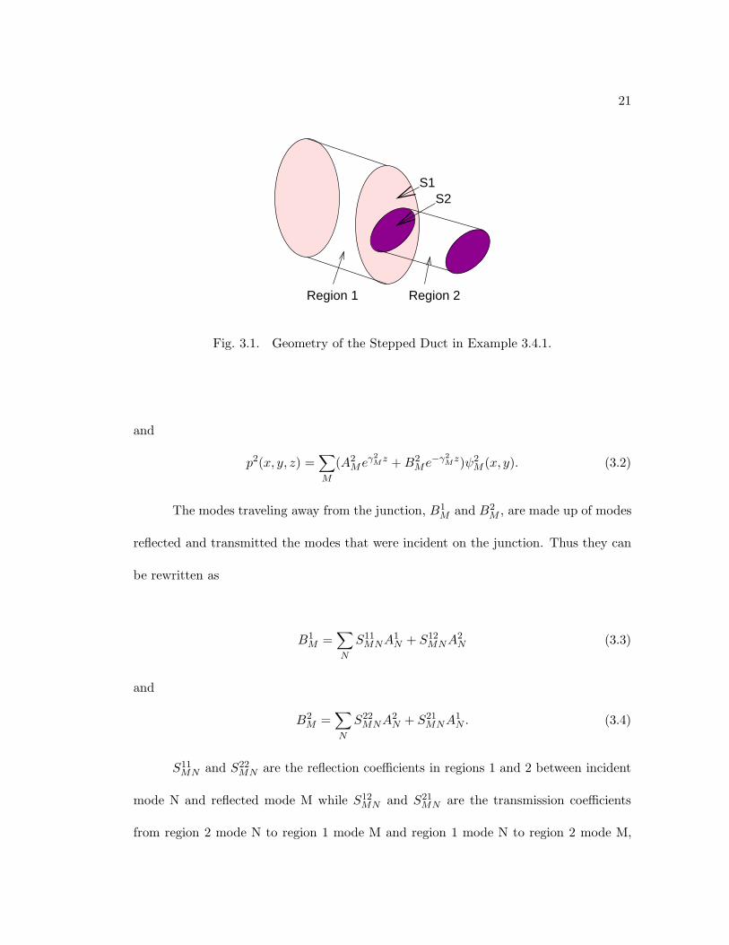
21
S1S2
Region 1 Region 2
Fig. 3.1. Geometry of the Stepped Duct in Example 3.4.1.
and
p2(x, y, z) =∑M
(A2Me
γ2M z +B2
Me−γ2
Mz)ψ2M (x, y). (3.2)
The modes traveling away from the junction, B1M and B2
M , are made up of modes
reflected and transmitted the modes that were incident on the junction. Thus they can
be rewritten as
B1M =
∑N
S11MNA
1N + S12
MNA2N (3.3)
and
B2M =
∑N
S22MNA
2N + S21
MNA1N . (3.4)
S11MN and S22
MN are the reflection coefficients in regions 1 and 2 between incident
mode N and reflected mode M while S12MN and S21
MN are the transmission coefficients
from region 2 mode N to region 1 mode M and region 1 mode N to region 2 mode M,
22
respectively. By solving for S11MN and S21
MN the reflection and transmission coefficients for
a constriction are found. By solving for S22MN and S12
MN the reflection and transmission
coefficients for an expansion are found.
Using equations 3.3 and 3.4, equation 3.1 and 3.2 can be rewritten as
p1(x, y, z) =∑M
(A1Me−γ1
M z +∑N
[S11MNA
1N + S12
MNA2N ]eγ
2M z)ψ1
M (x, y) (3.5)
and
p2(x, y, z) =∑M
(A2Me
γ2M z +
∑N
[S22MNA
2N + S21
MNA1N ]e−γ
2M z)ψ2
M (x, y). (3.6)
Using Euler’s equation, the velocity in the +z direction is found to be
u1z(x, y, z) =
∑M
Y 1M (A1
Me−γ1
M z −∑N
[S11MNA
1N + S12
MNA2N ]eγ
1M z)ψ1
M (x, y) (3.7)
and
u2z(x, y, z) =
∑M
Y 2M (−A2
Meγ2M z +
∑N
[S22MNA
2N + S21
MNA1N ]e−γ
2M z)ψ2
M (x, y). (3.8)
At z = 0 the pressure and normal velocity are continuous across S2 so
p1(x, y) =∑M
(A1M +
∑N
[S11MNA
1N + S12
MNA2N ])ψ1
M (x, y)
= p2(x, y) =∑M
(A2M +
∑N
[S22MNA
2N + S21
MNA1N ])ψ2
M (x, y) (3.9)
23
and
u1z(x, y) =
∑M
Y 1M (A1
M −∑N
[S11MNA
1N + S12
MNA2N ])ψ1
M (x, y)
= u2z(x, y) =
∑M
Y 2M (−A2
M +∑N
[S22MNA
2N + S21
MNA1N ])ψ2
M (x, y). (3.10)
If equation 3.9 is multiplied by ψ2R and integrated across the interface (S2), the
sum on the right hand side will be eliminated because of the orthogonality of the modes
in region 2. Equation 3.9 then becomes
∑M
HRM (A1M +
∑N
[S11MNA
1N + S12
MNA2N ]) = A2
R +∑N
[S22RNA
2N + S21
RNA1N ] (3.11)
where the coupling constant HRM is defined as
HRM =
∫∫S2
ψ2R(x, y)ψ1
M (x, y)dxdy∫∫S2
(ψ2R(x, y))2dxdy
=∫∫S2
ψ2R(x, y)ψ1
M (x, y)dxdy. (3.12)
The normal velocity at z = 0 over the area S3 (part of S1 outside of S2) is zero.
From this constraint it follows that for any function f(x, y)
∫∫S2
u1z(x, y, 0)f(x, y)dxdy =
∫∫S1
u1z(x, y, 0)f(x, y)dxdy. (3.13)
If equation 3.10 is multiplied by ψ1R and integrated across the interfaces (S2) and
if the integration over the left side of equation 3.10 is extended using equation 3.13, the
24
sum on the left hand side will be eliminated because of the orthogonality of the modes
in region 1. Thus equation 3.10 reduces to
Y 1M(A1
R−∑N
[S11RNA
1N+S12
RNA2N ]) =
∑M
HMRY2M (−A2
M+∑N
[S22MNA
2N+S21
MNA1N ]). (3.14)
These equations can be rewritten using the matrix notation of chapter 2. First
however, a few new matrices must be defined; let the scattering matrix S and the coupling
matrix H be defined as
Sµν =
Sµν00 Sµν01 · · ·
Sµν10 Sµν11 · · ·...
.... . .
H =
H00 H01 · · ·
H10 H11 · · ·...
.... . .
. (3.15)
With these definitions equations 3.11 and 3.14 become
H(I + S11)A1 + HS12A2 = (I + S22)A2 + S21A1 (3.16)
and
Y 1(I − S11)A1 − Y 1S12A2 = HT Y 2(S22 − I)A2 + HT Y 2S21A1. (3.17)
These equations hold for arbitrary A1 and A2. By setting A2 = 0 one finds
S11 = (Y 1 + HT Y 2H)−1(Y 1 − HT Y 2H) (3.18)
25
and
S21 = H(I + S11). (3.19)
By setting A1 = 0 and defining the generalized inverse of H as G = (HT H)−1HT
one finds
S22 = 2(Y 2 + GT Y 1G)−1(Y 2 − GT Y 1G) (3.20)
and
S12 = G(I + S22). (3.21)
Equations 3.18 and 3.20 have a very familiar form. The equations for S11 and S22
are the same form as that for reflection of a plane wave in a medium with a characteristic
admittance ya incident on a medium with an admittance yb, i.e. z = (ya− yb)/(ya + yb).
Thus one can identify HT Y 2H as the equivalent impedance matrix seen from region 1
looking toward the discontinuity and GT Y 1G as the equivalent impedance as seen from
region 2 looking toward the discontinuity. Since Y 1 and Y 2 are diagonal matrices one
can also see that all the mutual modal coupling is contained in the H and HT matrices.
3.2 Numerical Considerations
In numerically solving for Sµν , the summations (and hence the matrix size) must
be finite. As indicated in chapter 2, in order for the truncated solution to converge toward
the exact value, the number of modes in each region is not arbitrary - a certain ratio is
required to achieve convergence. As an example, consider region 1 to be a rectangular
duct of dimensions a1, b1 and region 2 to be a rectangular duct of dimensions a2, b2. If
26
N1x and N1y denote the number of modes in the x direction and y direction of region
1, and N2x and N2y the number of modes in the x and y direction in region 2 the
ratios are N1x/N2x = a1/a2 and N1y/N2y = b1/b2. Thus the total number of modes is
N1 = N1xN1y in region 1 and N2 = N2xN2y in region 2.
In addition, there are alternate forms of equations 3.18 to 3.20. The form used
above was chosen because it helps to show the physics of the problem by drawing analo-
gies to known situations. However, it requires computing several N1xN1 matrix inver-
sions, one being a generalized inverse which can often be difficult. Defining Z1c as (Y 1)−1,
equations 3.18 to 3.20 can be rewritten as
S11 = I − Z1c H
T Y 2S21, (3.22)
S21 = 2(HZ1c H
T Y 2 + I)−1H, (3.23)
S22 = (HZ1c H
T Y 2 + I)−1(HZ1c HY
2 − I), (3.24)
and
S12 = Z1c H
T (I − S22). (3.25)
In this form only one inversion of an N2xN2 matrix is required (recall that
N2 < N1 and note that Zc isn’t counted because Y is diagonal in inversion is simple).
The computational workload has been extremely reduced by eliminating several time
consuming matrix inversions and since the matrix being inverted is smaller, accuracy
should be increased - especially if the matrices being inverted are close to singular.
27
y
z
x
a1
1b b2
a2δ ε
Fig. 3.2. Geometry of a General Rectangular Stepped Duct
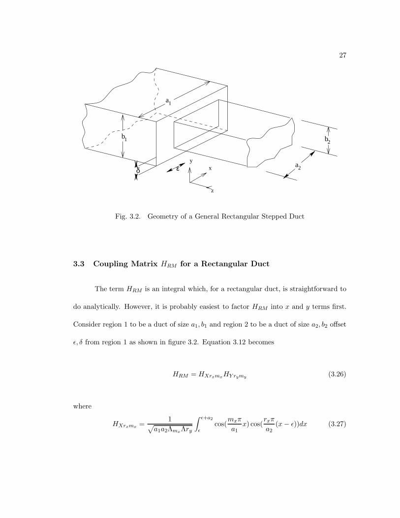
3.3 Coupling Matrix HRM for a Rectangular Duct
The term HRM is an integral which, for a rectangular duct, is straightforward to
do analytically. However, it is probably easiest to factor HRM into x and y terms first.
Consider region 1 to be a duct of size a1, b1 and region 2 to be a duct of size a2, b2 offset
ε, δ from region 1 as shown in figure 3.2. Equation 3.12 becomes
HRM = HXrxmxHY rymy (3.26)
where
HXrxmx =1√
a1a2ΛmxΛry
∫ ε+a2
εcos(
mxπ
a1x) cos(
rxπ
a2(x− ε))dx (3.27)
28
and
HY rymy =1√
b1b2ΛmyΛry
∫ δ+b2
δcos(
myπ
b1y) cos(
ryπ
b2(y − δ))dy. (3.28)
In general, the integrals yield
HXrxmx =a2√a1a2 mx
π√
ΛmxΛrx
(−1)rx sin(mxπa1(a2 + ε))− sin(mxπa1
ε)(mxa2)2 − (rxa1)2
(3.29)
HY rymy =b2√b1b2 my
π√
ΛmxΛrx
(−1)ry sin(myπb1 (b2 + δ)) − sin(myπb1 δ)(myb2)2 − (ryb1)2
. (3.30)
When mx = rxa1/a2 the first integral yields
HXrxmx =√a1
a2cos(
mxπ
a1ε). (3.31)
When my = ryb1/b2 the second integral yields
HY rymy =
√b2b1
cos(myπ
b1δ). (3.32)
It should be noted that equation 3.31 holds even when mx = 0 and 3.32 holds
even when my = 0.
When mx = 0 but rx 6= 0 or my = 0 but ry 6= 0
HRM = 0. (3.33)

29
3.4 Examples
To demonstrate applications of the theory, two examples will be developed. First
is an asymmetric duct. This duct is commonly used for example problems in microwave
theory [28, 41]. The second problem is a symmetric duct which is probably a more
common size change found in industrial ducting systems. It has also been investigated
by microwave waveguide researchers [56, 57].
3.4.1 An Asymmetric Stepped Duct
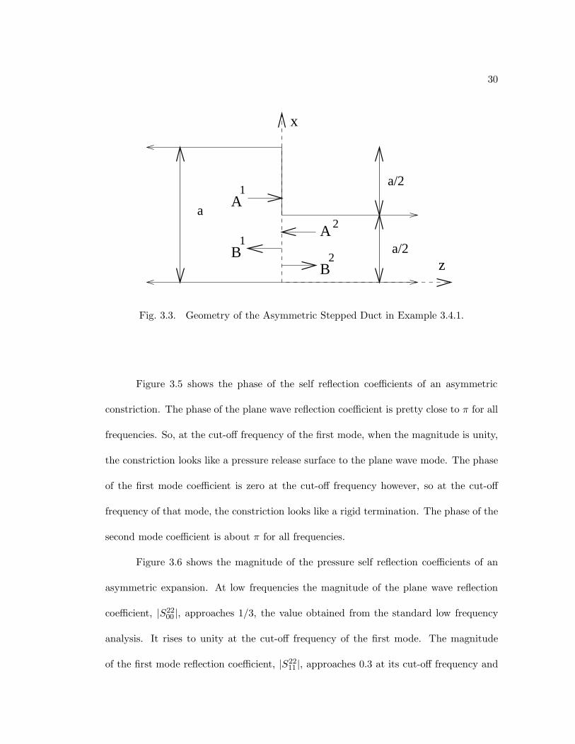
Consider a duct as shown in figure 3.3. At z = 0 the duct changes from a duct
with 0 < x < a to a duct with 0 < x < a/2. To simplify the calculation, only a
discontinuity in the x direction is considered. Since there is no discontinuity in the y
direction, all the y dependence and terms in the problem will drop out.
Figure 3.4 shows the magnitude of the pressure self reflection coefficients of an
asymmetric constriction. The magnitude of the plane wave coefficient, |S1100 |, approaches
1/3 at low frequencies. That is the expected value obtained from the standard low
frequency analysis which can be used as a limiting check for the theory presented here.
The plane wave coefficient increase with frequency, reaching unity at ka = π, the cut-off
frequency of the first horizontal mode. At that frequency the magnitude of the first
mode self reflection coefficient, |S1111 |, is also unity. Above the cut-off frequency of the
mode the first mode coefficient magnitude quickly drops to a small value. The reflection
coefficient of the second mode, |S1122 |, is not unity at its cut-off frequency, but is about
1/3. Above the cut-off frequency it rises.
30
x
z
2A
B2B
1
A1
a
a/2
a/2
Fig. 3.3. Geometry of the Asymmetric Stepped Duct in Example 3.4.1.
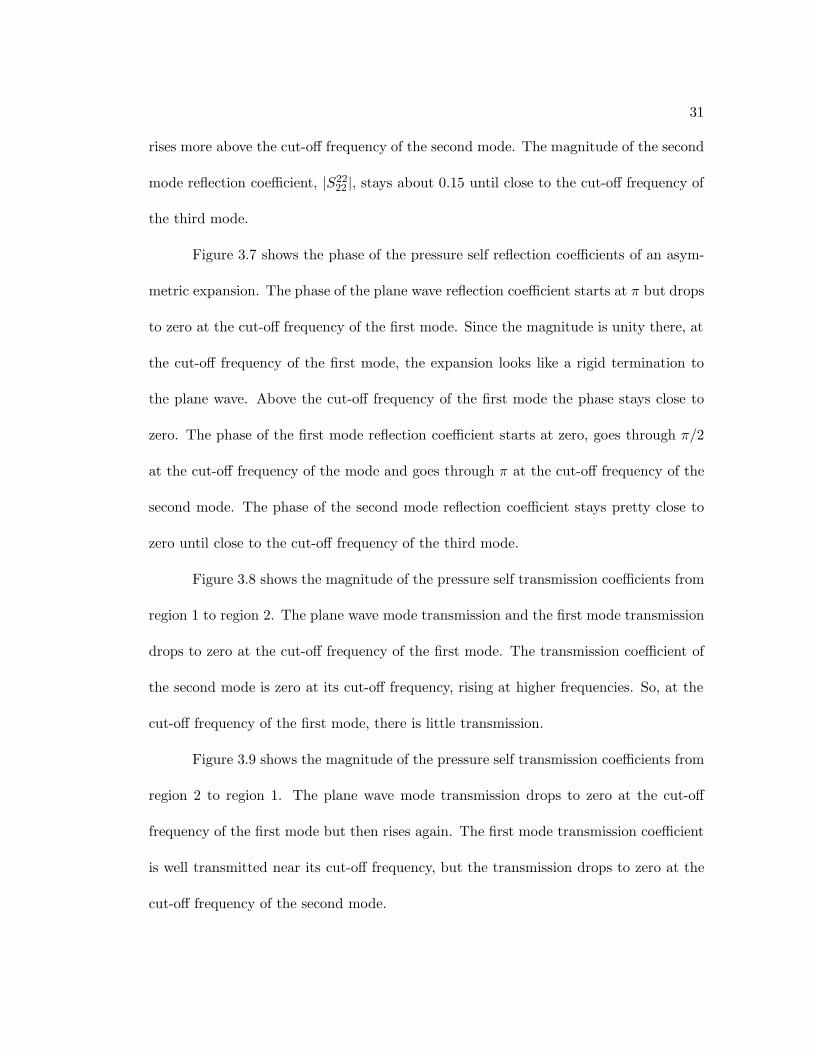
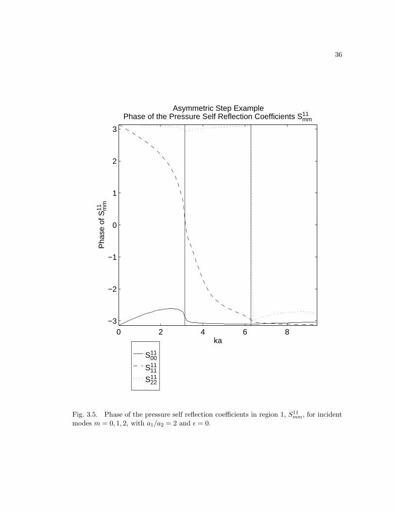
Figure 3.5 shows the phase of the self reflection coefficients of an asymmetric
constriction. The phase of the plane wave reflection coefficient is pretty close to π for all
frequencies. So, at the cut-off frequency of the first mode, when the magnitude is unity,
the constriction looks like a pressure release surface to the plane wave mode. The phase
of the first mode coefficient is zero at the cut-off frequency however, so at the cut-off
frequency of that mode, the constriction looks like a rigid termination. The phase of the
second mode coefficient is about π for all frequencies.
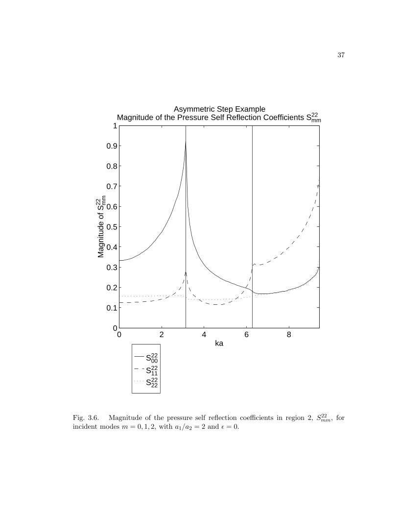
Figure 3.6 shows the magnitude of the pressure self reflection coefficients of an
asymmetric expansion. At low frequencies the magnitude of the plane wave reflection
coefficient, |S2200 |, approaches 1/3, the value obtained from the standard low frequency
analysis. It rises to unity at the cut-off frequency of the first mode. The magnitude
of the first mode reflection coefficient, |S2211 |, approaches 0.3 at its cut-off frequency and
31
rises more above the cut-off frequency of the second mode. The magnitude of the second
mode reflection coefficient, |S2222 |, stays about 0.15 until close to the cut-off frequency of
the third mode.
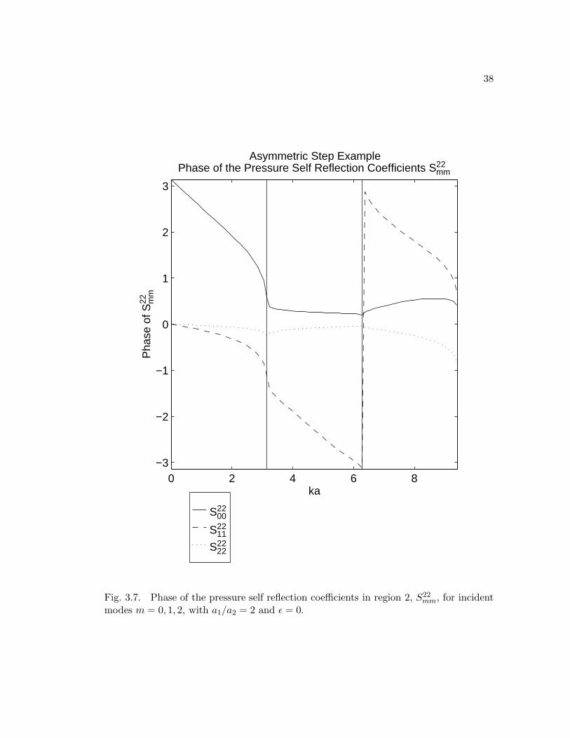
Figure 3.7 shows the phase of the pressure self reflection coefficients of an asym-
metric expansion. The phase of the plane wave reflection coefficient starts at π but drops
to zero at the cut-off frequency of the first mode. Since the magnitude is unity there, at
the cut-off frequency of the first mode, the expansion looks like a rigid termination to
the plane wave. Above the cut-off frequency of the first mode the phase stays close to
zero. The phase of the first mode reflection coefficient starts at zero, goes through π/2
at the cut-off frequency of the mode and goes through π at the cut-off frequency of the
second mode. The phase of the second mode reflection coefficient stays pretty close to
zero until close to the cut-off frequency of the third mode.
Figure 3.8 shows the magnitude of the pressure self transmission coefficients from
region 1 to region 2. The plane wave mode transmission and the first mode transmission
drops to zero at the cut-off frequency of the first mode. The transmission coefficient of
the second mode is zero at its cut-off frequency, rising at higher frequencies. So, at the
cut-off frequency of the first mode, there is little transmission.
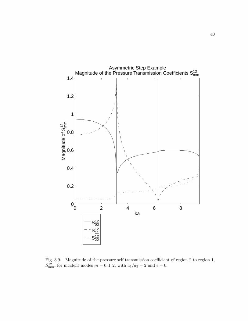
Figure 3.9 shows the magnitude of the pressure self transmission coefficients from
region 2 to region 1. The plane wave mode transmission drops to zero at the cut-off
frequency of the first mode but then rises again. The first mode transmission coefficient
is well transmitted near its cut-off frequency, but the transmission drops to zero at the
cut-off frequency of the second mode.

32
Figure 3.10 shows the magnitude of the mutual pressure reflection and transmis-
sion coefficients from the plane wave mode to the first mode. There is significant coupling
to the first mode from a plane wave mode incident from region 1 and region 2. All the
coefficients have local peaks near the cut-off frequency of the first mode. The mutual
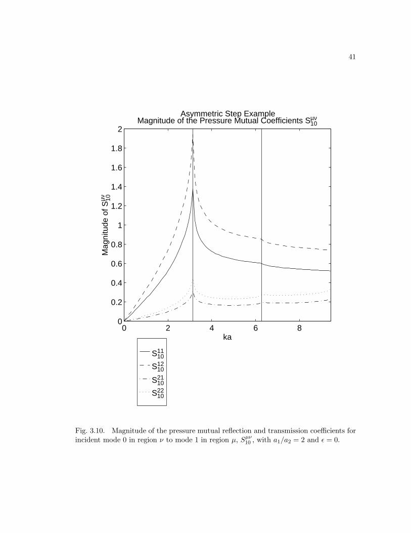
reflection coefficient, S1110 , is larger than unity, which at first might seem to be impossible,
but only the self reflection coefficients cannot exceed unity, mutual reflection coefficients
can exceed unity if the coefficient is for a plane wave mode to a higher order mode be-
cause the plane wave mode carries more energy than the higher order modes with the
same amplitude, thus the pressure coupling coefficient may be greater than unity but
the energy transfer coefficient will not be. With coupling coefficients approaching and
exceeding unity, it is easy to see that modal coupling is not negligible.
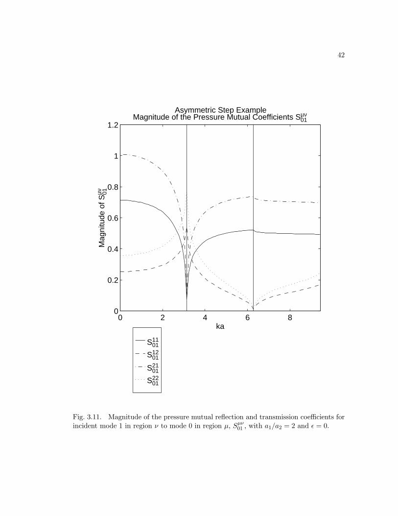
Figure 3.11 shows the magnitude of the mutual pressure reflection and trans-
mission coefficients from the first mode to the plane wave mode. The reflection and
transmission coefficients in region 1 go to zero at the cut-off frequency of the first mode.
The reflection and transmission coefficients in region 2 are largest at the cut-off frequency
of the first mode but they go to zero at the cut-off frequency of the second mode. There
is significant coupling from the first mode to the plane wave mode incident in region 2
near the cut-off frequency of the first mode and in region I above the cut-off frequency
of the first mode.
Figure 3.12 shows the magnitude of the mutual pressure reflection and transmis-
sion coefficients from the plane wave mode to the second mode. All the coefficients have
a local peak at the cut-off frequency of the first mode. Recall however, that the second
33
mode can not yet propagate at that frequency. All the coefficients rise again at the
cut-off frequency of the third mode. The overall level is quite low however.
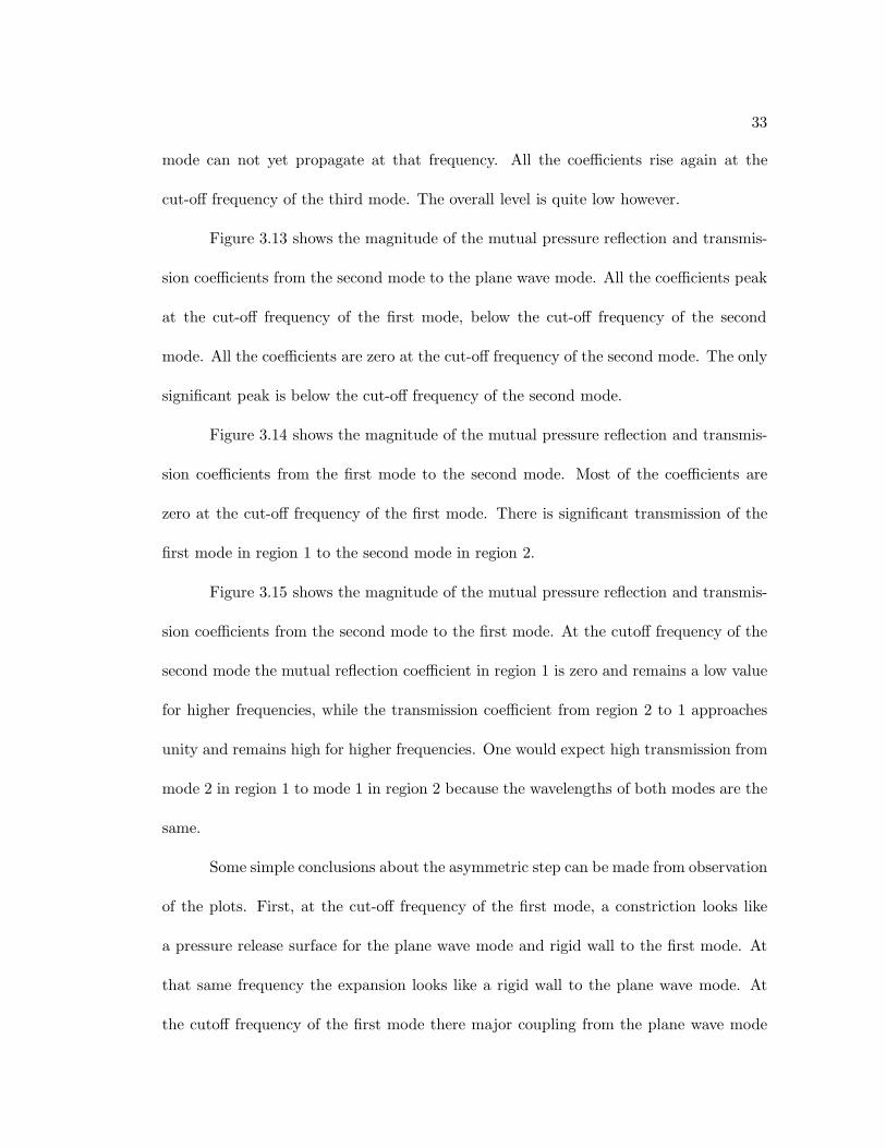
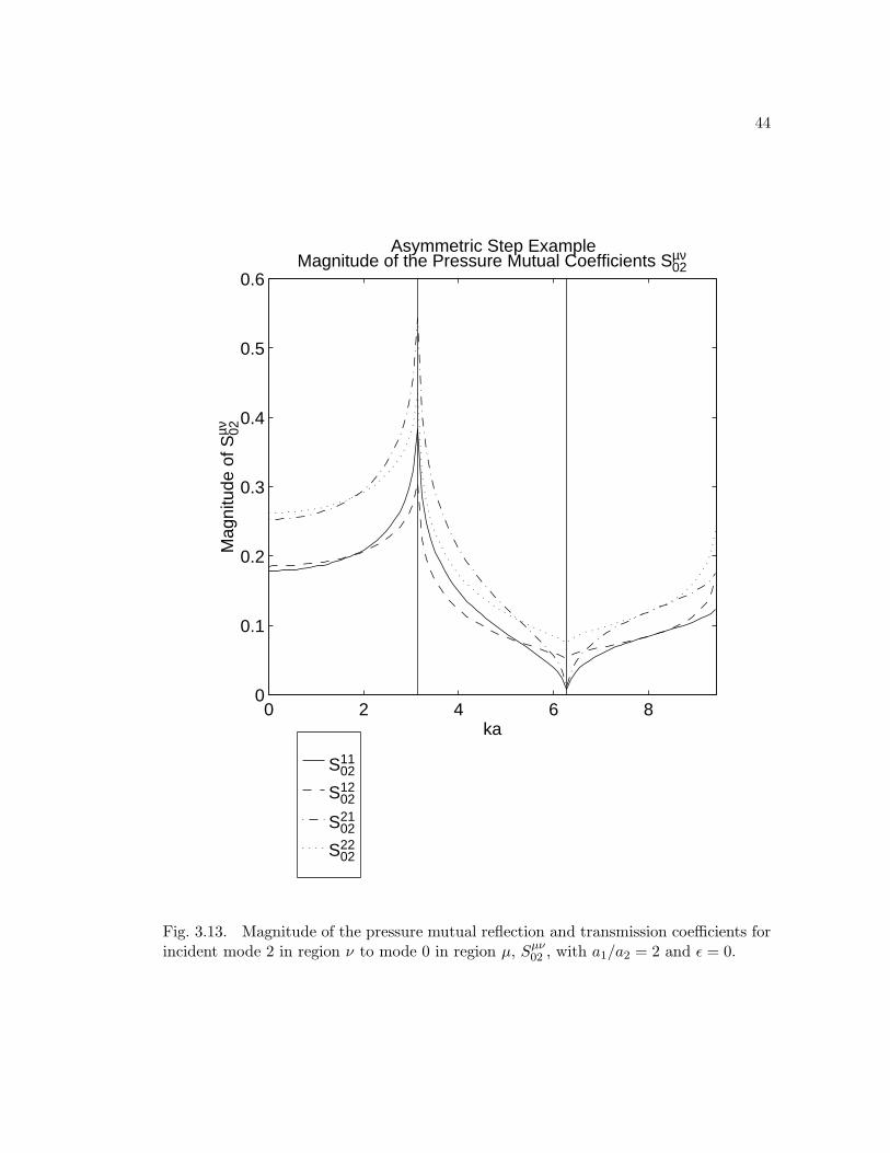
Figure 3.13 shows the magnitude of the mutual pressure reflection and transmis-
sion coefficients from the second mode to the plane wave mode. All the coefficients peak
at the cut-off frequency of the first mode, below the cut-off frequency of the second
mode. All the coefficients are zero at the cut-off frequency of the second mode. The only
significant peak is below the cut-off frequency of the second mode.
Figure 3.14 shows the magnitude of the mutual pressure reflection and transmis-
sion coefficients from the first mode to the second mode. Most of the coefficients are
zero at the cut-off frequency of the first mode. There is significant transmission of the
first mode in region 1 to the second mode in region 2.
Figure 3.15 shows the magnitude of the mutual pressure reflection and transmis-
sion coefficients from the second mode to the first mode. At the cutoff frequency of the
second mode the mutual reflection coefficient in region 1 is zero and remains a low value
for higher frequencies, while the transmission coefficient from region 2 to 1 approaches
unity and remains high for higher frequencies. One would expect high transmission from
mode 2 in region 1 to mode 1 in region 2 because the wavelengths of both modes are the
same.
Some simple conclusions about the asymmetric step can be made from observation
of the plots. First, at the cut-off frequency of the first mode, a constriction looks like
a pressure release surface for the plane wave mode and rigid wall to the first mode. At
that same frequency the expansion looks like a rigid wall to the plane wave mode. At
the cutoff frequency of the first mode there major coupling from the plane wave mode

34
in region 1 and 2 to the first mode in region 1. At higher frequencies the first mode
in region 1 couples well to the plane wave mode in regions 1 and 2. By comparing the
magnitudes of the mutual reflection coefficients to the magnitudes of the self reflection
coefficients, it is clear that modal coupling is significant and important.

35
S1100
S1111
S1122
0 2 4 6 80
0.1
0.2
0.3
0.4
0.5
0.6
0.7
0.8
0.9
1
ka
Magnitude of the Pressure Self Reflection Coefficients S11mm
Aymmetric Step ExampleM
agni
tude
of S
11 mm
Fig. 3.4. Magnitude of the pressure self reflection coefficients in region 1, S11mm, for
incident modes m = 0, 1, 2, with a1/a2 = 2 and ε = 0.
36
S1100
S1111
S1122
0 2 4 6 8−3
−2
−1
0
1
2
3
ka
Phase of the Pressure Self Reflection Coefficients S11mm
Asymmetric Step ExampleP
hase
of S
11 mm
Fig. 3.5. Phase of the pressure self reflection coefficients in region 1, S11mm, for incident
modes m = 0, 1, 2, with a1/a2 = 2 and ε = 0.
37
S2200
S2211
S2222
0 2 4 6 80
0.1
0.2
0.3
0.4
0.5
0.6
0.7
0.8
0.9
1
ka
Magnitude of the Pressure Self Reflection Coefficients S22mm
Asymmetric Step ExampleM
agni
tude
of S
22 mm
Fig. 3.6. Magnitude of the pressure self reflection coefficients in region 2, S22mm, for
incident modes m = 0, 1, 2, with a1/a2 = 2 and ε = 0.
38
S2200
S2211
S2222
0 2 4 6 8−3
−2
−1
0
1
2
3
ka
Phase of the Pressure Self Reflection Coefficients S22mm
Asymmetric Step ExampleP
hase
of S
22 mm
Fig. 3.7. Phase of the pressure self reflection coefficients in region 2, S22mm, for incident
modes m = 0, 1, 2, with a1/a2 = 2 and ε = 0.

39
S2100
S2111
S2122
0 2 4 6 80
0.1
0.2
0.3
0.4
0.5
0.6
0.7
0.8
0.9
1
ka
Magnitude of the Pressure Transmission Coefficients S21mm
Asymmetric Step ExampleM
agni
tude
of S
21 mm
Fig. 3.8. Magnitude of the pressure self transmission coefficient of region 1 to region 2,S21mm, for incident modes m = 0, 1, 2, with a1/a2 = 2 and ε = 0.
40
S1200
S1211
S1222
0 2 4 6 80
0.2
0.4
0.6
0.8
1
1.2
1.4
ka
Magnitude of the Pressure Transmission Coefficients S12mm
Asymmetric Step ExampleM
agni
tude
of S
12 mm
Fig. 3.9. Magnitude of the pressure self transmission coefficient of region 2 to region 1,S12mm, for incident modes m = 0, 1, 2, with a1/a2 = 2 and ε = 0.
41
S1110
S1210
S2110
S2210
0 2 4 6 80
0.2
0.4
0.6
0.8
1
1.2
1.4
1.6
1.8
2
ka
Magnitude of the Pressure Mutual Coefficients Sµν10
Asymmetric Step ExampleM
agni
tude
of S
µν 10
Fig. 3.10. Magnitude of the pressure mutual reflection and transmission coefficients forincident mode 0 in region ν to mode 1 in region µ, Sµν10 , with a1/a2 = 2 and ε = 0.
42
S1101
S1201
S2101
S2201
0 2 4 6 80
0.2
0.4
0.6
0.8
1
1.2
ka
Magnitude of the Pressure Mutual Coefficients Sµν01
Asymmetric Step ExampleM
agni
tude
of S
µν 01
Fig. 3.11. Magnitude of the pressure mutual reflection and transmission coefficients forincident mode 1 in region ν to mode 0 in region µ, Sµν01 , with a1/a2 = 2 and ε = 0.

43
S1120
S1220
S2120
S2220
0 2 4 6 80
0.05
0.1
0.15
0.2
0.25
0.3
0.35
ka
Magnitude of the Pressure Mutual Coefficients Sµν20
Asymmetric Step ExampleM
agni
tude
of S
µν 20
Fig. 3.12. Magnitude of the pressure mutual reflection and transmission coefficients forincident mode 0 in region ν to mode 2 in region µ, Sµν20 , with a1/a2 = 2 and ε = 0.
44
S1102
S1202
S2102
S2202
0 2 4 6 80
0.1
0.2
0.3
0.4
0.5
0.6
ka
Magnitude of the Pressure Mutual Coefficients Sµν02
Asymmetric Step ExampleM
agni
tude
of S
µν 02
Fig. 3.13. Magnitude of the pressure mutual reflection and transmission coefficients forincident mode 2 in region ν to mode 0 in region µ, Sµν02 , with a1/a2 = 2 and ε = 0.

45
S1121
S1221
S2121
S2221
0 2 4 6 80
0.1
0.2
0.3
0.4
0.5
0.6
0.7
0.8
0.9
1
ka
Magnitude of the Pressure Mutual Coefficients Sµν 21
Asymmetric Step ExampleM
agni
tude
of S
µν 21
Fig. 3.14. Magnitude of the pressure mutual reflection and transmission coefficients forincident mode 1 in region ν to mode 2 in region µ, Sµν21 , with a1/a2 = 2 and ε = 0.

46
S1112
S1212
S2112
S2212
0 2 4 6 80
0.1
0.2
0.3
0.4
0.5
0.6
0.7
0.8
0.9
1
ka
Magnitude of the Pressure Mutual Coefficients Sµν12
Asymmetric Step ExampleM
agni
tude
of S
µν 12
Fig. 3.15. Magnitude of the mutual pressure reflection and transmission coefficients forincident mode 2 in region ν to mode 1 in region µ, Sµν12 , with a1/a2 = 2 and ε = 0.
47
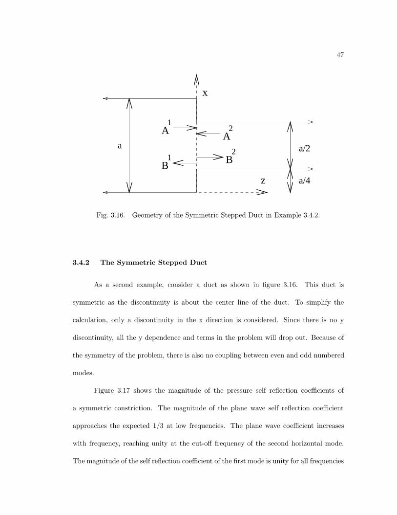
x
z
A
B1
1
A
B2
2
a/4
a/2a
Fig. 3.16. Geometry of the Symmetric Stepped Duct in Example 3.4.2.
3.4.2 The Symmetric Stepped Duct
As a second example, consider a duct as shown in figure 3.16. This duct is
symmetric as the discontinuity is about the center line of the duct. To simplify the
calculation, only a discontinuity in the x direction is considered. Since there is no y
discontinuity, all the y dependence and terms in the problem will drop out. Because of
the symmetry of the problem, there is also no coupling between even and odd numbered
modes.
Figure 3.17 shows the magnitude of the pressure self reflection coefficients of
a symmetric constriction. The magnitude of the plane wave self reflection coefficient
approaches the expected 1/3 at low frequencies. The plane wave coefficient increases
with frequency, reaching unity at the cut-off frequency of the second horizontal mode.
The magnitude of the self reflection coefficient of the first mode is unity for all frequencies

48
between the cut-off frequencies of the first mode and the second mode. The magnitude of
self reflection coefficient of the second mode is unity at its cut-off frequency, but quickly
drops above it.
Figure 3.18 shows the phase of the pressure self reflection coefficients of a symmet-
ric constriction. The phase of plane wave coefficient is about π for all frequencies. Since
the magnitude is unity at the cutoff frequency of the first mode, the constriction looks
like a rigid wall to the plane wave mode, just like for the asymmetric duct. The phase
of the first mode reflection coefficient is zero at its cut-off frequency so the constriction
looks like a rigid wall at that frequency. The phase for the first mode coefficient is π at
the cutoff of the second mode, so at that frequency the constriction looks like a pressure
release surface. The phase of second mode coefficient is zero at the cut-off frequency of
the second mode, so the constriction looks like a rigid wall to the second mode at the
cut-off frequency.
Figure 3.19 shows the magnitude of the pressure self reflection coefficients of a
symmetric expansion. The magnitude of the plane wave reflection coefficient approaches
the expected 1/3 at low frequencies. The magnitude of plane wave coefficient increases
with frequency, reaching unity at the cut-off frequency of the second horizontal mode.
The magnitude of the first mode reflection coefficient approaches unity at the cut-off
frequency of the first and second modes. The magnitude of reflection coefficient of the
second mode is small for all frequencies.
Figure 3.20 shows the phase of the pressure self reflection coefficients of a sym-
metric expansion. The phase of plane wave coefficient starts at π and approaches zero
at the cut-off frequency of the second mode. So the expansion looks like a rigid wall
49
at the cut-off frequency of the second mode. The phase of the first mode coefficient is
zero at its cut-off frequency so the expansion looks like a rigid wall at that frequency.
The phase for the first mode coefficient is π at the cutoff of the second mode, so at that
frequency the expansion looks like a pressure release surface. The phase of second mode
approaches π/2 at the cut-off frequency of the second mode.
Figure 3.22 shows the magnitude of the pressure self transmission coefficients
from region 2 to region 1. The plane wave mode has high transmission until the cut-off
frequency of the second mode. The first mode is well transmitted at its cut-off frequency
but not at all at the cut-off frequency of the second mode. The second mode transmits
well at its cut-off frequency, but the transmission drops at higher frequencies.
Figure 3.21 shows the magnitude of the pressure self transmission coefficients from
region 1 to region 2. Again, the plane wave mode is well transmitted until the cut-off
frequency of the second mode. The first mode is not transmitted at its cut-off frequency,
but has very high transmission at the cut-off frequency of the second mode. Since the
magnitude of first mode self reflection coefficient in region 1 was unity between the cut-
off of the first and second modes, the change in the transmission coefficient is indicative
of the change in phase of the reflection coefficient. At the cut-off frequency of the second
mode the plane wave and second mode do not transmit well.
Figure 3.23 shows the mutual coupling coefficients from plane wave mode to the
second mode. The plot shows that there is very significant coupling for reflected and
transmitted second modes for a plane wave incident from region 1, but little coupling
for a plane wave incident from region 2.
50
Figure 3.24 shows the mutual coupling coefficients from the second mode to the
plane wave mode. The plot shows that at the cut-off frequency of the second mode
there is significant coupling for reflected and transmitted modes for a mode incident
from region 2. At higher frequencies there is significant coupling for modes incident in
region 1.
Some simple conclusions about the symmetric step can be made from observation
of the plots. First, at the cut-off frequency of the first mode, a constriction looks like a
pressure release surface for the plane wave mode and rigid wall to the first mode and the
second mode. At that same frequency the expansion looks like a rigid wall to the plane
wave mode and a pressure release surface to the first mode. Again, there is significant
modal coupling above the cut-off frequency of the first mode, with coupling coefficients
greater than unity at some frequencies.
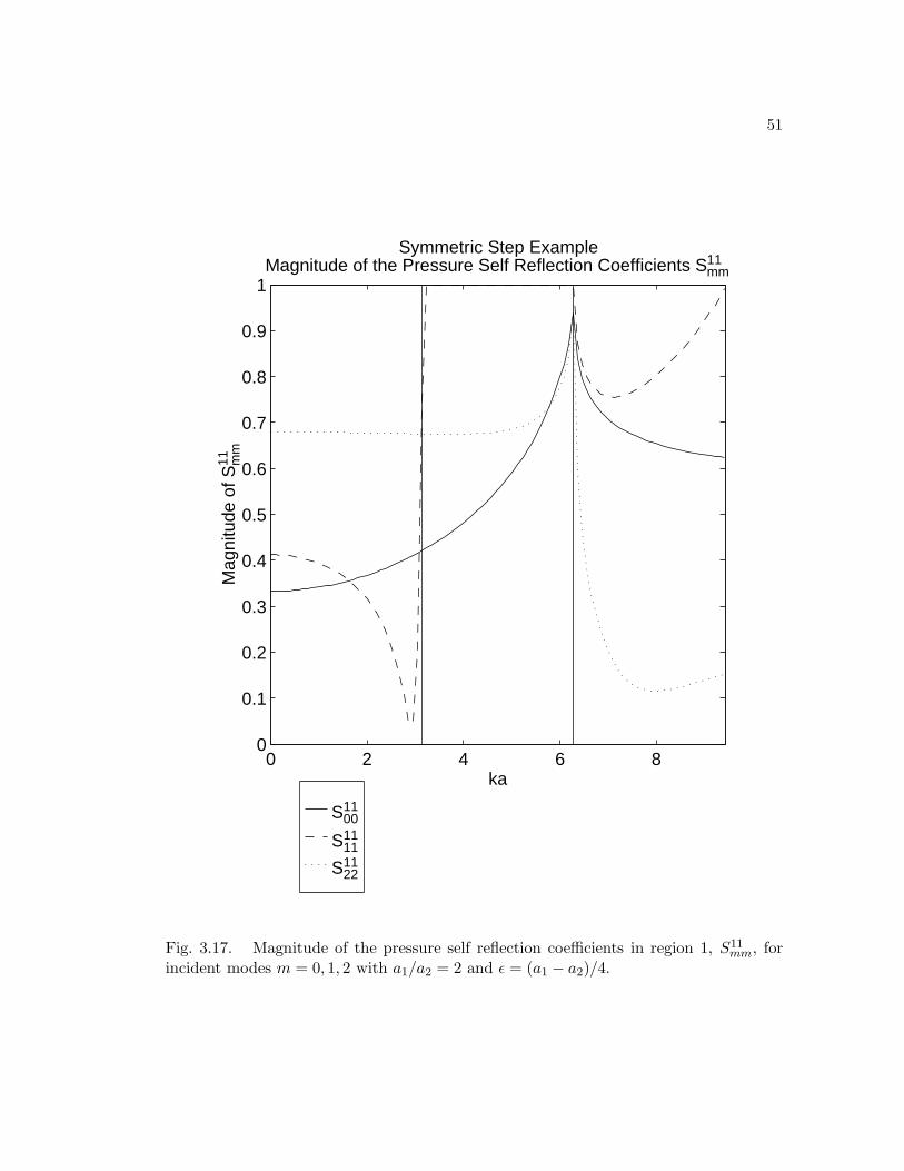
51
S1100
S1111
S1122
0 2 4 6 80
0.1
0.2
0.3
0.4
0.5
0.6
0.7
0.8
0.9
1
ka
Magnitude of the Pressure Self Reflection Coefficients S11mm
Symmetric Step ExampleM
agni
tude
of S
11 mm
Fig. 3.17. Magnitude of the pressure self reflection coefficients in region 1, S11mm, for
incident modes m = 0, 1, 2 with a1/a2 = 2 and ε = (a1 − a2)/4.
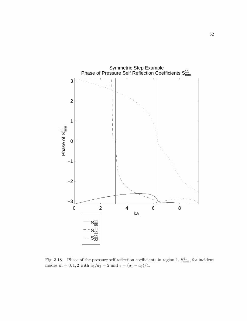
52
S1100
S1111
S1122
0 2 4 6 8−3
−2
−1
0
1
2
3
ka
Phase of Pressure Self Reflection Coefficients S11mm
Symmetric Step ExampleP
hase
of S
11 mm
Fig. 3.18. Phase of the pressure self reflection coefficients in region 1, S11mm, for incident
modes m = 0, 1, 2 with a1/a2 = 2 and ε = (a1 − a2)/4.
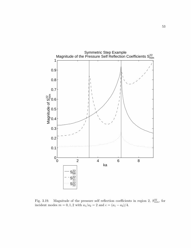
53
S2200
S2211
S2222
0 2 4 6 80
0.1
0.2
0.3
0.4
0.5
0.6
0.7
0.8
0.9
1
ka
Magnitude of the Pressure Self Reflection Coefficients S22mm
Symmetric Step ExampleM
agni
tude
of S
22 mm
Fig. 3.19. Magnitude of the pressure self reflection coefficients in region 2, S22mm, for
incident modes m = 0, 1, 2 with a1/a2 = 2 and ε = (a1 − a2)/4.
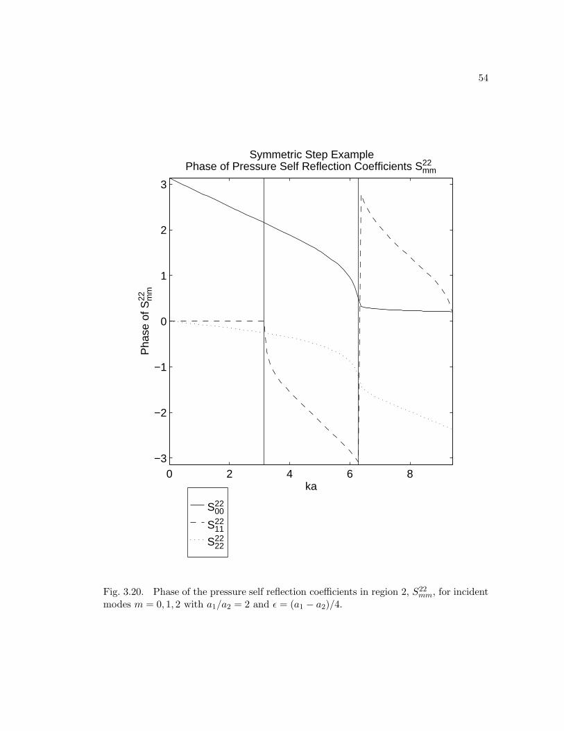
54
S2200
S2211
S2222
0 2 4 6 8−3
−2
−1
0
1
2
3
ka
Phase of Pressure Self Reflection Coefficients S22mm
Symmetric Step ExampleP
hase
of S
22 mm
Fig. 3.20. Phase of the pressure self reflection coefficients in region 2, S22mm, for incident
modes m = 0, 1, 2 with a1/a2 = 2 and ε = (a1 − a2)/4.

55
S2100
S2111
S2122
0 2 4 6 80
0.2
0.4
0.6
0.8
1
1.2
ka
Magnitude of the Pressure Transmission Coefficients S21mm
Symmetric Step ExampleM
agni
tude
S21 m
m
Fig. 3.21. Magnitude of the pressure self transmission coefficient of region 1 to region2, S21
mm, for incident modes m = 0, 1, 2, with a1/a2 = 2 and ε = (a1 − a2)/4.
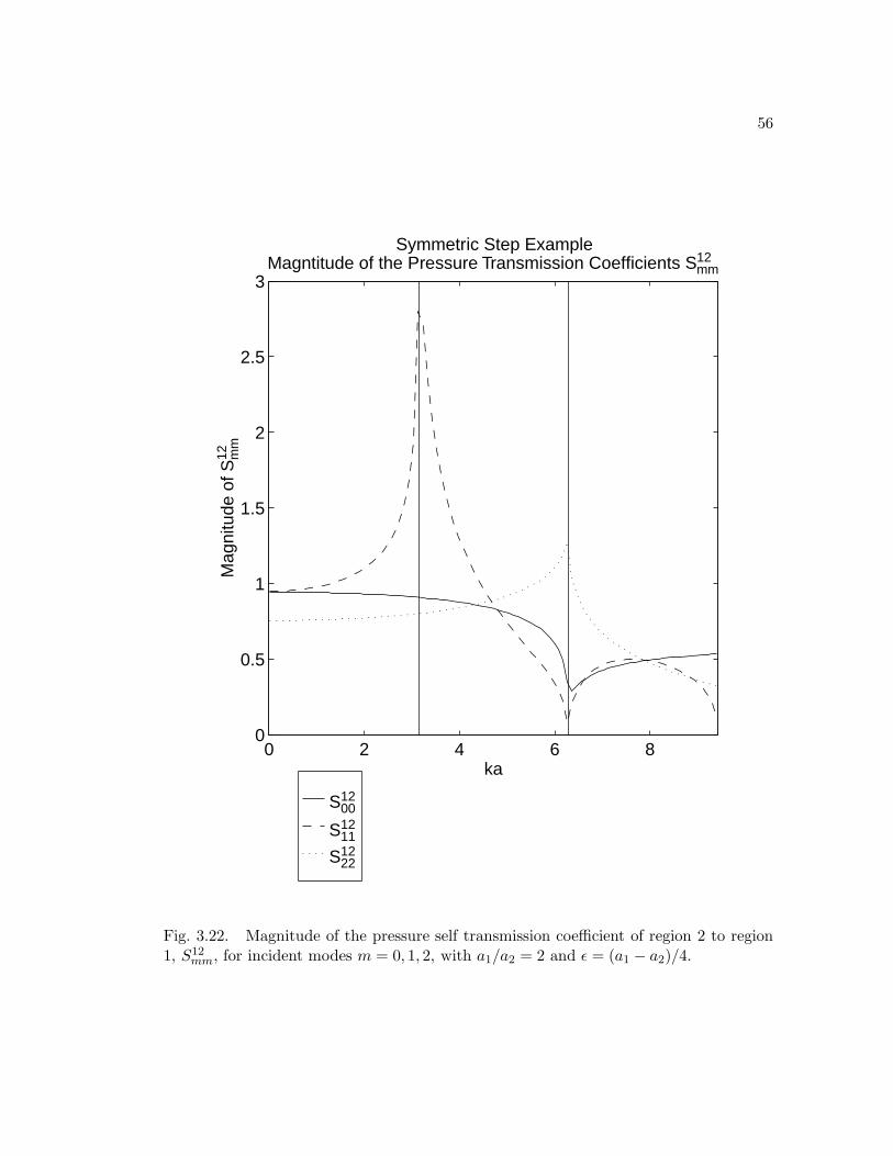
56
S1200
S1211
S1222
0 2 4 6 80
0.5
1
1.5
2
2.5
3
ka
Magntitude of the Pressure Transmission Coefficients S12mm
Symmetric Step ExampleM
agni
tude
of S
12 mm
Fig. 3.22. Magnitude of the pressure self transmission coefficient of region 2 to region1, S12
mm, for incident modes m = 0, 1, 2, with a1/a2 = 2 and ε = (a1 − a2)/4.
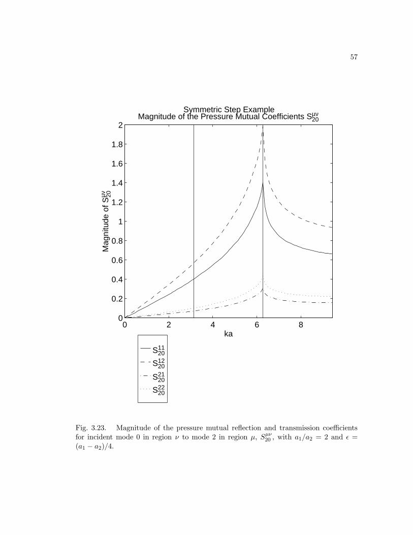
57
S1120
S1220
S2120
S2220
0 2 4 6 80
0.2
0.4
0.6
0.8
1
1.2
1.4
1.6
1.8
2
ka
Magnitude of the Pressure Mutual Coefficients Sµν20
Symmetric Step ExampleM
agni
tude
of S
µν 20
Fig. 3.23. Magnitude of the pressure mutual reflection and transmission coefficientsfor incident mode 0 in region ν to mode 2 in region µ, Sµν20 , with a1/a2 = 2 and ε =(a1 − a2)/4.
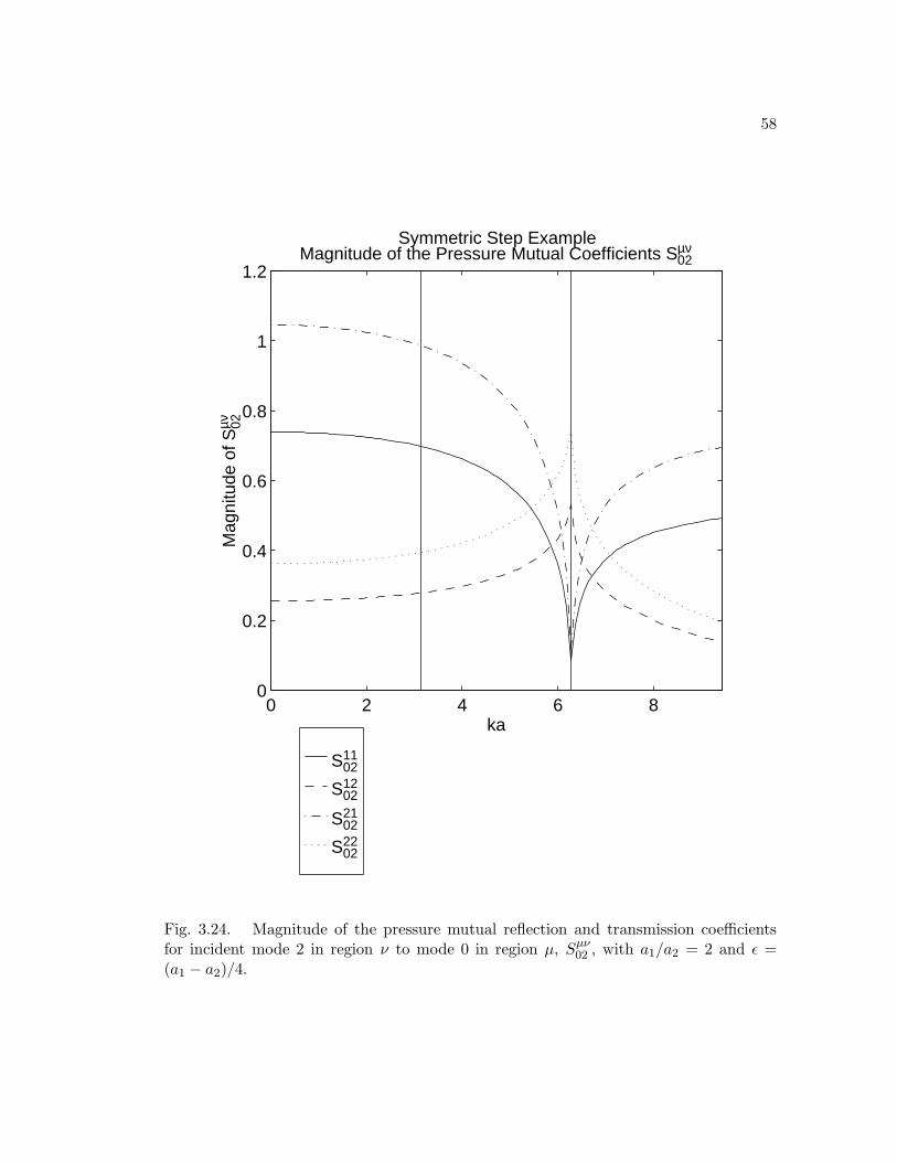
58
S1102
S1202
S2102
S2202
0 2 4 6 80
0.2
0.4
0.6
0.8
1
1.2
ka
Magnitude of the Pressure Mutual Coefficients Sµν02
Symmetric Step ExampleM
agni
tude
of S
µν 02
Fig. 3.24. Magnitude of the pressure mutual reflection and transmission coefficientsfor incident mode 2 in region ν to mode 0 in region µ, Sµν02 , with a1/a2 = 2 and ε =(a1 − a2)/4.

59
Chapter 4
Modal Scattering at Junctions
Just as the step discontinuity was an important part of acoustical networks and
filters, so is the junction. A junction is a general region to which two or more ducts are
connected. A duct bend can be described as a sort of junction with two ports. Expansion
and constriction chambers could also be described as junctions with two ports. This
chapter will derive a basic theory for determining reflection and transmission between
the different ports of a junction.
4.1 General Junction Theory
Consider a multi-port junction as shown in figure 4.1. Each port is a duct, each
with its own propagating modes. When a given mode in one duct is incident upon the
junction, part of the mode is reflected back into that same mode in that duct, part is
reflected back into other modes in that duct, and part is transmitted into various modes
in other ducts.
If the Green’s function for the junction region is known, an integral relation
between the pressure and the velocity at the duct-junction interface can be developed.
The pressure and velocity can be written in terms of the modes and hence an integral
relation between the modes can be established.
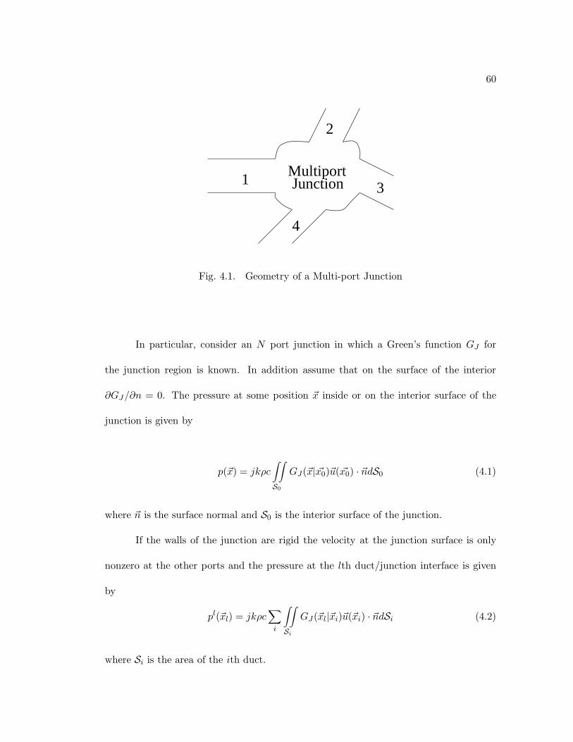
60
4
1
2
3JunctionMultiport
Fig. 4.1. Geometry of a Multi-port Junction
In particular, consider an N port junction in which a Green’s function GJ for
the junction region is known. In addition assume that on the surface of the interior
∂GJ/∂n = 0. The pressure at some position ~x inside or on the interior surface of the
junction is given by
p(~x) = jkρc
∫∫S0
GJ(~x| ~x0)~u( ~x0) · ~ndS0 (4.1)
where ~n is the surface normal and S0 is the interior surface of the junction.
If the walls of the junction are rigid the velocity at the junction surface is only
nonzero at the other ports and the pressure at the lth duct/junction interface is given
by
pl(~xl) = jkρc∑i
∫∫Si
GJ(~xl|~xi)~u(~xi) · ~ndSi (4.2)
where Si is the area of the ith duct.
61
The pressure in each duct can be expanded into a modal series of the form
pl(xl, yl, vl) =∑M
(AlMe−γlM zl +Bl
MeγlM zl)ψlM (xl, yl) (4.3)
where xl, yl, and zl are locally defined coordinates such that the interface between the
duct and junction is defined as zl = 0 and the direction of +zl is towards the junction.
Given pl as above, the normal velocity ulz can be found, using Euler’s equation,
to be
ulz =∑M
Y lM (AlMe
−γlMzl −BlMe
γlM zl)ψlM (xl, yl) (4.4)
where Y lM is the characteristic modal admittance of the Mth mode in the lth port.
Using equations 4.3 and 4.4 in equation 4.2 results in the relation
∑M
(AlM +BlM )ψlM (xl, yl) = jkρc
∑i
∑M
Y iM (AiM −Bi
M )
×∫∫Si
GJ (xl, yl|xi, yi)
∣∣∣∣∣∣∣ zl=0zi=0
ψiM (xi, yi)dxidyi. (4.5)
Multiplying equation 4.5 by ψlR and integrating over Sl yields
AlR +BlR =
∑i
∑M
Y iM (AiM −Bi
M )Z liRM (4.6)
where
Z liRM = jkρc
∫∫Sl
∫∫Si
GJ (xl, yl|xi, yi)
∣∣∣∣∣∣∣ zl=0zi=0

62
×ψlR(xl, yl)ψiM (xi, yi)dxidyidxldyl. (4.7)
Z liRM is the mutual modal impedance between port i mode M and port l mode
R.
Since impedance is the ratio of pressure to velocity, the reason for identifying
Z liRM as a modal impedance is because the left hand side of equation 4.6 is the amplitude
of the pressure of the Rth mode in the lth port while the right hand size is the sum of
Z liRM times the velocity of the Mth mode in the ith port.
Equation 4.6 has Y iM multiplying Z liRM . Since Y i
M is the characteristic modal
admittance of the Mth mode in port i, the multiplication is normalization of the mutual
modal impedance by the characteristic modal impedance of that port. Thus, it makes
sense to define the normalized modal impedance ηliRM as
ηliRM = Y iMZ
liRM . (4.8)
In matrix form equation 4.6 becomes
Al + Bl = ηli(Ai − Bi). (4.9)
The reflected waves Bl can be rewritten in terms of the incident waves and scat-
tering parameters in the form
Bl =∑q
SlqAq (4.10)
63
and equation 4.9 becomes
Al +∑q
SlqAq = ηli(Ai −∑q
SiqAq). (4.11)
Defining the super matrices
A =
A0
A1
...
Y =
Y 0
Y 1
...
S =
S00 S01 · · ·
S10 S11 · · ·...
.... . .
η =
η00 η01 · · ·
η10 η11 · · ·...
.... . .
(4.12)
equation 4.11 can be reduced to
(I + S)A = η(I − S)A (4.13)
from which the scattering matrix S is found to be
S = (η + I)−1(η − I). (4.14)
This form of the equation for the scattering matrix is the same as the normalized
form of the plane wave reflection coefficient at a planar change of impedance.
4.2 Examples
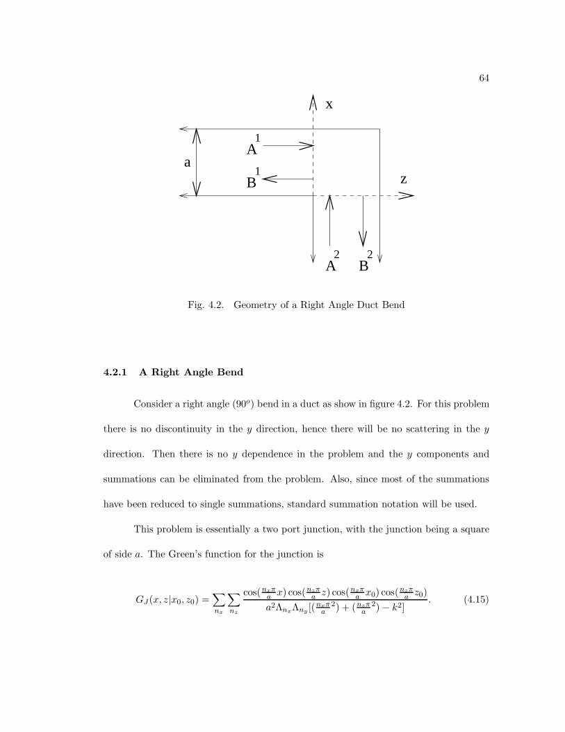
64
z
x
aB
1
A1
A B2 2
Fig. 4.2. Geometry of a Right Angle Duct Bend
4.2.1 A Right Angle Bend
Consider a right angle (90o) bend in a duct as show in figure 4.2. For this problem
there is no discontinuity in the y direction, hence there will be no scattering in the y
direction. Then there is no y dependence in the problem and the y components and
summations can be eliminated from the problem. Also, since most of the summations
have been reduced to single summations, standard summation notation will be used.
This problem is essentially a two port junction, with the junction being a square
of side a. The Green’s function for the junction is
GJ (x, z|x0, z0) =∑nx
∑nz
cos(nxπa x) cos(nzπa z) cos(nxπa x0) cos(nzπa z0)a2ΛnxΛny [(nxπa
2) + (nzπa2)− k2]
. (4.15)
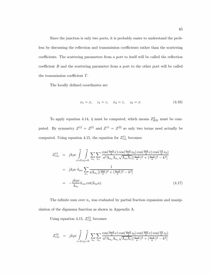
65
Since the junction is only two ports, it is probably easier to understand the prob-
lem by discussing the reflection and transmission coefficients rather than the scattering
coefficients. The scattering parameters from a port to itself will be called the reflection
coefficient R and the scattering parameter from a port to the other port will be called
the transmission coefficient T .
The locally defined coordinates are
x1 = x, z1 = z, x2 = z, z2 = x. (4.16)
To apply equation 4.14, η must be computed, which means ZilRM must be com-
puted. By symmetry Z12 = Z21 and Z11 = Z22 so only two terms need actually be
computed. Using equation 4.15, the equation for Z11rm becomes
Z11rm = jkρc
a∫x=0
a∫x0=0
∑nx
∑nz
cos(nxπa x) cos(nxπa x0) cos(mπa x) cos(rπa x0)a3ΛnxΛnz
√ΛmΛr[(nxπa )2 + (nzπa )2 − k2]
= jkρc δmr∑nz
1aΛnz [(
mπa )2 + (nzπa )2 − k2]
= −jkρckm
δrm cot(kma). (4.17)
The infinite sum over nz was evaluated by partial fraction expansion and manip-
ulation of the digamma function as shown in Appendix A.
Using equation 4.15, Z12rm becomes
Z12rm = jkρc
a∫z=0
a∫x0=0
∑nx
∑nz
cos(nxπa x) cos(nxπa z0) cos(mπa x) cos(rπa z0)a3ΛnxΛnz
√ΛmΛr[(nxπa )2 + (nzπa )2 − k2]

66
= jkρc1
a√
ΛmΛr[(mπa )2 + (rπa )2 − k2]. (4.18)
Given the impedance matrix Z and hence the normalized impedance matrix η,
the reflection and transmission coefficients can now be calculated from equation 4.14
Figures 4.3 to 4.8 are the magnitude of the pressure reflection and transmission
coefficients of a right angle bend. They match the theoretical results of Shepherd and
Cabelli [59] who used a finite element technique instead of a modal technique. Also
shown in figures 4.3 to 4.7 are the experimental measurements of Shepherd and Cabelli
which match the theory very well.
Figure 4.3 shows the magnitude of the pressure reflection coefficients for an inci-
dent plane wave. At low frequencies |R00| approaches zero as expected. Also as expected,
|R20| and |R10| are zero since there is no coupling at low frequencies. As frequency
increases all the reflection coefficients are rising. However, remember that until the fre-
quency is above the cut-off of a given mode, it is evanescent and even if part of the plane
wave is reflected into it, it cannot propagate. At the cut-off frequency of the first mode
the junction region has a resonance and the self reflection coefficient approaches unity
because the impedance of the junction is very high. The coupling coefficients go to zero.
Again when the frequency reaches the cut-off frequency of the second mode there is a
junction region resonance and the plane wave reflection coefficient goes to unity. While
it appears that |R00| is always larger than the coupling coefficients above the cut-off
frequency of the first mode, there is a significant part of the plane wave coupled into
67
the other modes. The theoretical results match the experimental measurements of Shep-
herd and Cabelli quite well, with most of the theoretical values within the error of the
measurements.
In figure 4.4 are shown the magnitudes of the pressure reflection coefficients for
an incident first mode. At the cut-off frequency of the first mode the magnitude of the
first mode self reflection coefficient |R11| is unity, and there is no coupling into the other
modes. Unlike the plane wave mode, the coupling coefficient |R01| is larger than the self
reflection coefficient |R11| in the region of ka =5, showing that there is significant modal
coupling at higher frequencies. Again the theoretical results are within the error of the
measurements.
In figure 4.5 are shown the magnitudes of the pressure self and mutual reflection
coefficients for an incident second mode. Close to the cut-off frequency of the third mode
the coupling between the second and first mode is greater than the self reflection of the
second mode. The measurements do not match the theory quite as well as for the lower
order mode reflection coefficients. This is to be expected as measurements of the second
mode are more difficult than for the lower modes.
Figure 4.6 shows the magnitude of the pressure transmission coefficients for an
incident plane wave. At low frequencies |T00| approaches unity as expected. At the
cut-off frequency of the first mode, the plane wave is not transmitted (as expected since
|R00| = 1) but the transmission coefficient |T10| is quite large, showing that much of
the plane wave is transmitted to the first mode. This is also expected as at the cut-
off frequency of the first mode, the trace wavenumber of the incident plane wave mode
matches the trace wavenumber of a transmitted first mode. At the cut-off frequency of
68
the second mode |T20| gets large while |T01| and |T00| are small. Again the plane wave
is converted into the mode which is just above its cut-off frequency because the trace
wavenumbers match. The theoretical results are within the error of the measurements.
Figure 4.7 shows the magnitudes of the pressure transmission coefficients for an
incident first mode. At the cut-off frequency of the first mode there is no transmission
- as expected because |R11| = 1 at that frequency. At the cut-off frequency of the
second mode the |T12| is large again indicating significant modal coupling. Most of the
theoretical results are within the error of the measurements.
Figure 4.8 shows the magnitudes of the pressure transmission coefficients for an
incident second mode. The results are as expected, there is no self transmission at
the cut-off frequency of the second mode mode and good coupling to the first mode
which matches the trace wavenumber of the incident second mode. No experimental
measurements were available for comparison.
As a result of the above plots, some simple conclusions can be made. First, at
the cut-off frequency of a mode, the self reflection coefficient is unity while the self
transmission coefficient is zero. This is because of the resonances of the junction region.
Perhaps more importantly, the coupling between a mode and the next higher mode is
very large when the frequency is just above the cut-off frequency of the higher mode.
This is because of trace wavenumber matching of the incident mode and transmitted
mode. The plane wave mode will couple greatly into whichever mode is just above its
cut-off frequency. It is quite clear that a right angle bend will significantly change the
modal structure of the propagating wave at all but very low frequencies.

69
The theoretical results match the experimental results of Shepherd and Cabelli
quite well. The theory is verified and can be used with confidence to determine the
scattering parameters of other types of junctions.
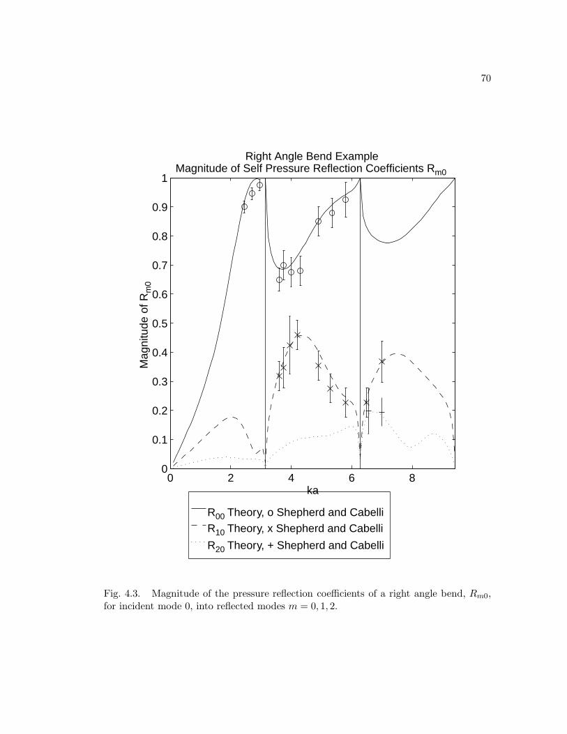
70
R00 Theory, o Shepherd and CabelliR10 Theory, x Shepherd and Cabelli
R20 Theory, + Shepherd and Cabelli
0 2 4 6 80
0.1
0.2
0.3
0.4
0.5
0.6
0.7
0.8
0.9
1
ka
Magnitude of Self Pressure Reflection Coefficients Rm0
Right Angle Bend ExampleM
agni
tude
of R
m0
Fig. 4.3. Magnitude of the pressure reflection coefficients of a right angle bend, Rm0,for incident mode 0, into reflected modes m = 0, 1, 2.
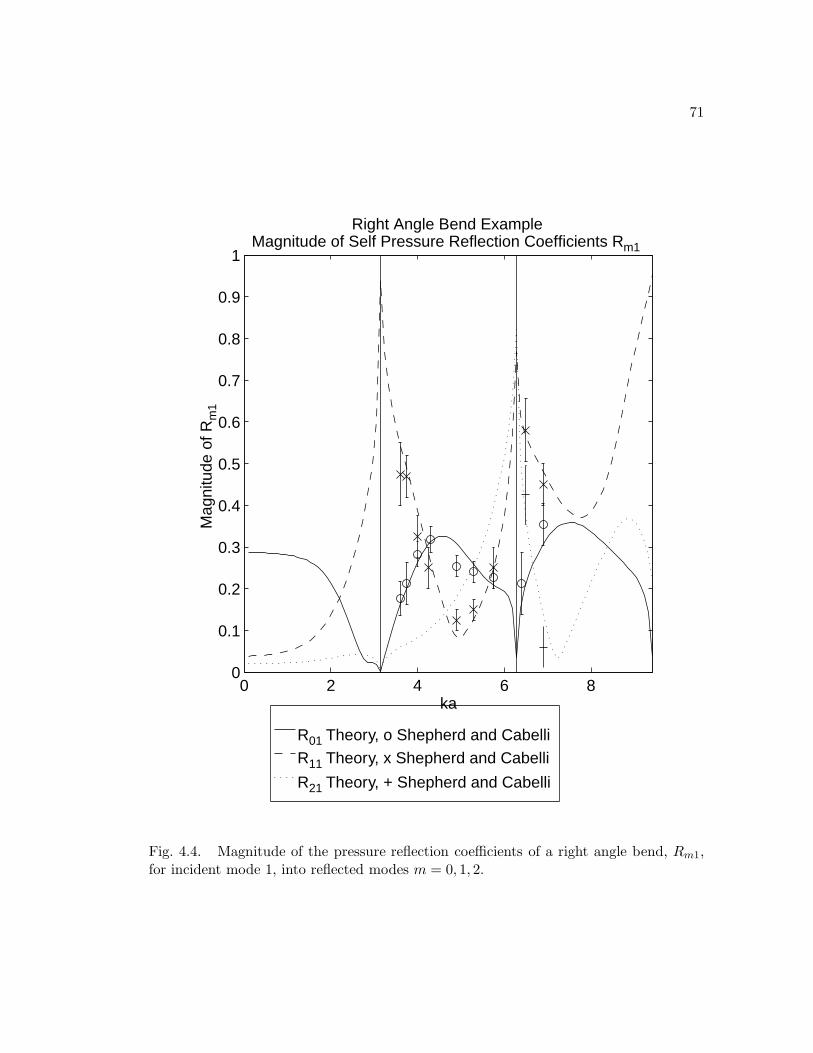
71
R01 Theory, o Shepherd and CabelliR11 Theory, x Shepherd and Cabelli
R21 Theory, + Shepherd and Cabelli
0 2 4 6 80
0.1
0.2
0.3
0.4
0.5
0.6
0.7
0.8
0.9
1
ka
Magnitude of Self Pressure Reflection Coefficients Rm1
Right Angle Bend ExampleM
agni
tude
of R
m1
Fig. 4.4. Magnitude of the pressure reflection coefficients of a right angle bend, Rm1,for incident mode 1, into reflected modes m = 0, 1, 2.
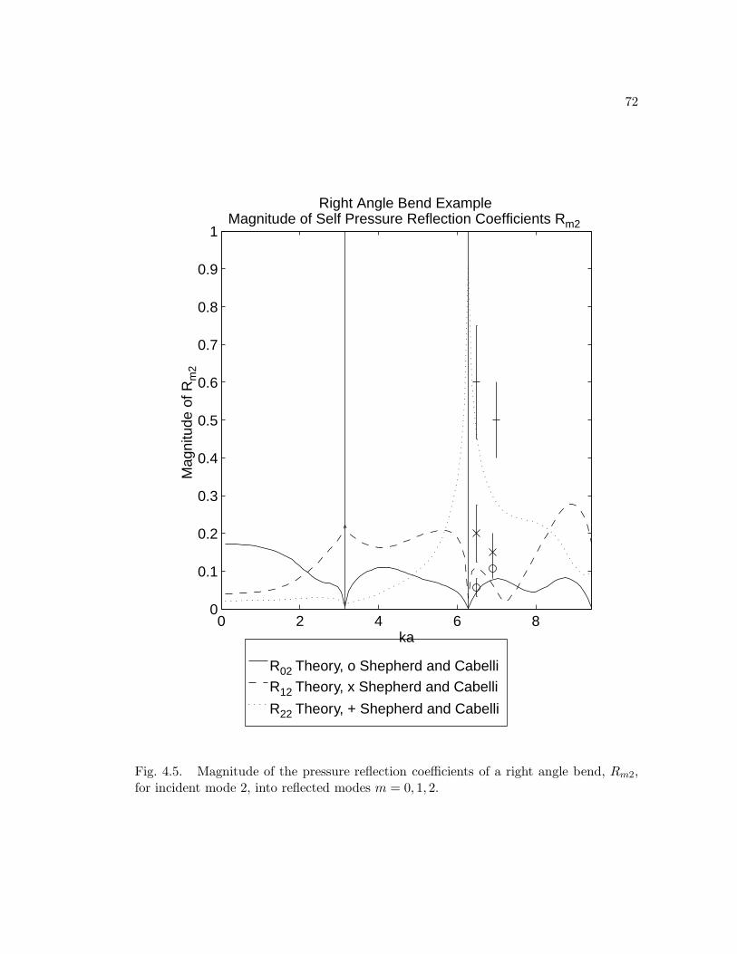
72
R02 Theory, o Shepherd and CabelliR12 Theory, x Shepherd and Cabelli
R22 Theory, + Shepherd and Cabelli
0 2 4 6 80
0.1
0.2
0.3
0.4
0.5
0.6
0.7
0.8
0.9
1
ka
Magnitude of Self Pressure Reflection Coefficients Rm2
Right Angle Bend ExampleM
agni
tude
of R
m2
Fig. 4.5. Magnitude of the pressure reflection coefficients of a right angle bend, Rm2,for incident mode 2, into reflected modes m = 0, 1, 2.

73
T00 Theory, o Shepherd and CabelliT10 Theory, x Shepherd and Cabelli
T20 Theory
0 2 4 6 80
0.2
0.4
0.6
0.8
1
1.2
1.4
ka
Magnitude of Pressure Transmission Coefficients Tm0
Right Angle Bend ExampleM
agni
tude
Tm
0
Fig. 4.6. Magnitude of the pressure transmission coefficients of a right angle bend, Tm0,for incident mode 0, into transmitted modes m = 0, 1, 2.
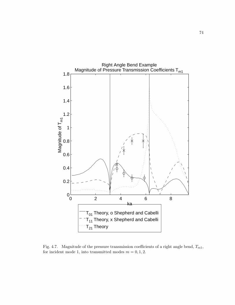
74
T01 Theory, o Shepherd and CabelliT11 Theory, x Shepherd and Cabelli
T21 Theory
0 2 4 6 80
0.2
0.4
0.6
0.8
1
1.2
1.4
1.6
1.8
ka
Magnitude of Pressure Transmission Coefficients Tm1
Right Angle Bend ExampleM
agni
tude
of T
m1
Fig. 4.7. Magnitude of the pressure transmission coefficients of a right angle bend, Tm1,for incident mode 1, into transmitted modes m = 0, 1, 2.
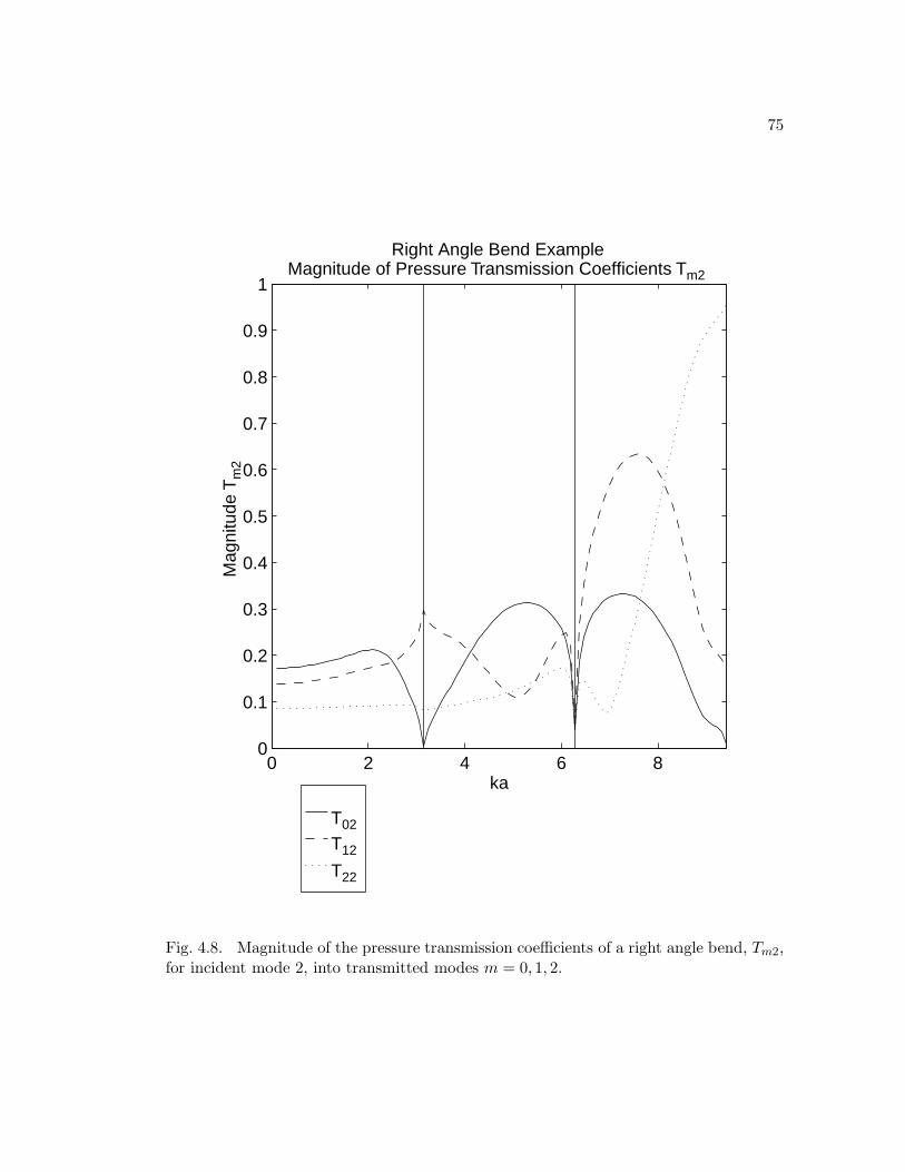
75
T02
T12
T22
0 2 4 6 80
0.1
0.2
0.3
0.4
0.5
0.6
0.7
0.8
0.9
1
ka
Magnitude of Pressure Transmission Coefficients Tm2
Right Angle Bend ExampleM
agni
tude
Tm
2
Fig. 4.8. Magnitude of the pressure transmission coefficients of a right angle bend, Tm2,for incident mode 2, into transmitted modes m = 0, 1, 2.

76
x
aB
1
A1
A B2 2
z
A3
B3
Fig. 4.9. Geometry of a T Junction
4.2.2 A T Junction
Consider the T junction as shown in 4.9. As in the previous example, there is
no y discontinuity thus y can be eliminated from the problem. The Green’s function
GJ is the same as the previous problem. In fact, the problem is so similar to the
previous example, that Z11 and Z12 are the same. By symmetry it is easy to see that
Z12 = Z21 = Z23 = Z32, Z33 = Z11 and Z13 = Z31.
For this problem the local coordinates are
x1 = x, z1 = z, x2 = z, z2 = x, x3 = x, z3 = (a− z). (4.19)
77
Z13rm is given by
Z13rm = jkρc
a∫x=0
a∫x0=0
∑nx
∑nz
cos(nxπa x) cos(nxπa x0) cos(nzπa a) cos(mπa x) cos(rπa x0)a3ΛnxΛnz
√ΛmΛr[(nxπa )2 + (nzπa )2 − k2]
= jkρc δrm∑nz
(−1)nz
aΛnz [(mπa )2 + (nzπa )2 − k2]
=jkρc δrm
2km[cot(
kma
2) + tan(
kma
2)]. (4.20)
Again in equation 4.20 the infinite summation was evalued by use of digamma
functions as shown in appendix A.
Figures 4.10 through 4.24 are the magnitudes of the reflection and transmission
coefficients for a T junction.
Figure 4.10 shows the magnitudes of pressure reflection coefficients for a plane
wave incident at one end of a T junction. At low frequencies the reflection coefficient
approaches the expected 1/3. As frequency rises the coefficient drops a bit but then
quickly rises to unity at the cut-off frequency of the first mode. At that frequency
there is no reflected coupling into other modes. This is because of a resonance of the
junction region. As the frequency goes up, the self reflection coefficient quickly drops
and the coupling coefficient between the plane wave and the first mode become larger.
At the cut-off frequency of the second mode the self reflection coefficient is zero. The
self reflection coefficient then rises to unity again at the cut-off frequency of the third
mode. At frequencies between the cut-off of the first and second mode the coupling from
the plane wave mode to the first mode is larger than the self reflection coefficient alone.

78
Figure 4.11 shows the magnitudes of the pressure reflection coefficients for a plane
wave incident from the side branch of the T. At low frequencies the reflection coefficient
approaches 1/3 and rises smoothly to unity at the cut-off frequency of the first mode.
There is not significant coupling between modes until close to the cut-off of the second
mode where significant coupling between the plane wave and first mode exists.
Figure 4.12 shows the magnitudes of the pressure transmission coefficient for the
plane wave mode from the side branch to the end. As expected, the low frequency limit
is 2/3. The self transmission coefficient drops to zero at the cut-off frequency of the
first mode. The coupling coefficient from the plane wave to the first mode is quite high
near the cut-off frequency but drops at the cut-off frequency. It is expected to be high
near the cut-off frequency from trace wavenumber matching, but the reason for the drop
at the cut-off frequency is unknown. At the cut-off frequency of the second mode the
coupling between the plane wave and the second mode is very high again (because of
trace wavenumber matching) while the self reflection coefficient is zero.
Figure 4.13 shows the magnitudes of the pressure transmission coefficients for the
plane wave from one end to the side branch of the T. At low frequencies the value of the
self transmission coefficient approaches the expected 2/3. At the cut-off frequency of the
first mode the plane mode is well coupled into the first mode while the self transmission
coefficient is zero. At the cut-off frequency of the second mode the plane wave mode is
well coupled into the second mode while the self transmission coefficient is zero. Again the
coupling to the higher order modes is expected because of trace wavenumber matching
at the cut-off frequencies of the modes. Clearly modal coupling is important.
79
Figure 4.14 shows the magnitudes of the pressure transmission coefficient for the
plane mode between the two ends of the T. The plane wave coefficient starts at 2/3 rises a
little and drops sharply to zero at the cut-off frequency of the first mode. This is because
of the cavity resonance which causes a high impedance to be seen to the incoming wave.
It then sharply rises with increasing frequency reaching unity at the cut-off frequency
of the second mode. The mutual coupling coefficients are both quite small compared to
the self coupling coefficients.
Figure 4.15 shows magnitudes of the pressure reflection coefficients for the first
mode incident at one end of the T. At the cut-off frequency for the mode, the reflec-
tion coefficient approaches unity. It wavers a bit and drops toward zero at the cut-off
frequency of the second mode. There is not significant coupling between modes until
the cut-off frequency of the second mode, where the coupling from the first mode to the
second mode is significant.
In figure 4.16 is shown the magnitudes of the pressure reflection coefficients for
the first mode incident at the side branch of the T. The self reflection coefficient is large
at the cut-off frequency of the first mode and stays pretty high for all frequencies.
Figure 4.17 shows the magnitudes of the pressure transmission coefficients for the
first mode from the side branch to the end. At the cut-off frequency of the first mode
the transmission coefficients are all zero since the reflection coefficient is unity. There is
significant coupling to the second mode near the cut-off frequency of the second mode.
Figure 4.18 shows the magnitudes of the pressure transmission coefficients for the
first mode from the end to the side branch of the T. At the cut-off frequency of the first

80
mode the transmission coefficients are all zero. Above the cut-off frequency of the second
mode the coupling coefficient between the first and second mode is very high.
Figure 4.19 shows the magnitudes of the pressure transmission coefficient for
the first mode between the two ends. There is little coupling between modes but the
transmission coefficient is small for frequencies near the cut-off frequency of the first
mode. The transmission coefficient approaches unity at the cut-off frequency of the
second mode.
Figure 4.20 shows the magnitudes of the pressure reflection coefficients for the
second mode incident at one end of the T. At the cut-off frequency of the second mode,
the self reflection coefficient approaches unity. There is little modal coupling.
Figure 4.21 shows the magnitudes of the pressure reflection coefficients for the
second mode incident at the side branch of the T. The self reflection coefficient approaches
unity at the cut-off frequency. Near the cut-off frequency of the third mode the mutual
reflection coefficient into the first mode is larger than the self reflection coefficient.
Figure 4.22 shows the magnitudes of the pressure transmission coefficients for the
second mode from the side branch to one end. The transmission coefficients are quite
complicated but there is not significant modal coupling.
Figure 4.23 shows the magnitudes of the pressure transmission coefficients for the
second mode from one end to the side branch of the T. Like the coefficient from the side
to the end, the overall coupling is low.
Figure 4.24 shows the magnitudes of the pressure transmission coefficients for the
second mode between the ends. There is little coupling between modes, but the self
transmission coefficient is high.
81
From the above plots one can conclude that in general the side branch does not
contribute heavily to modal coupling for transmission between the ends of the T, but it
does affect the self transmission of the modes between the ends of the T. There is very
significant coupling from the mode incident on the side branch to a another mode in
the ends just above its cut-off frequency because of trace wavenumber matching (just as
with the right angle bend). The modal coupling coefficient is often higher in magnitude
of than the self transmission coefficient and self reflection coefficient. Clearly modal
coupling with the side branch is very important.
In addition, one can see that, |S2100 |, the magnitude of the coupling from the side
branch plane wave mode to the plane wave mode in the T ends, drops to zero at the
cut-off frequency and is quite small at higher frequencies. This is important because it
says that a speaker mounted in the side of a duct is far less efficient at producing plane
wave modes at high frequencies - something of practical concern in active noise control
systems.
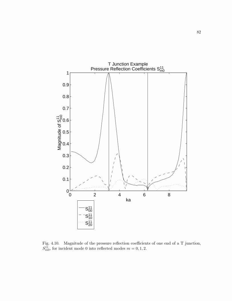
82
S1100
S1110
S1120
0 2 4 6 80
0.1
0.2
0.3
0.4
0.5
0.6
0.7
0.8
0.9
1
ka
Pressure Reflection Coefficients S11m0
T Junction ExampleM
agni
tude
of S
11 m0
Fig. 4.10. Magnitude of the pressure reflection coefficients of one end of a T junction,S11m0, for incident mode 0 into reflected modes m = 0, 1, 2.
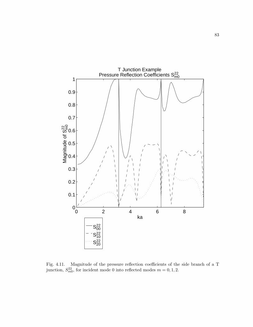
83
S2200
S2210
S2220
0 2 4 6 80
0.1
0.2
0.3
0.4
0.5
0.6
0.7
0.8
0.9
1
ka
Pressure Reflection Coefficients S22m0
T Junction ExampleM
agni
tude
of S
22 m0
Fig. 4.11. Magnitude of the pressure reflection coefficients of the side branch of a Tjunction, S22
m0, for incident mode 0 into reflected modes m = 0, 1, 2.

84
|S2100|
|S2110|
|S2120|
0 2 4 6 80
0.1
0.2
0.3
0.4
0.5
0.6
0.7
0.8
0.9
1
ka
Pressure Reflection Coefficients S21m0
T Junction|S
21 m0|
Fig. 4.12. Magnitude of the pressure transmission coefficients S21m0, from mode 0 in one
end of a T to modes m = 0, 1, 2 in the side branch.
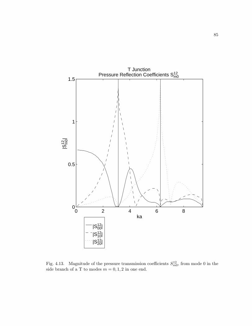
85
|S1200|
|S1210|
|S1220|
0 2 4 6 80
0.5
1
1.5
ka
Pressure Reflection Coefficients S12m0
T Junction|S
12 m0|
Fig. 4.13. Magnitude of the pressure transmission coefficients S12m0, from mode 0 in the
side branch of a T to modes m = 0, 1, 2 in one end.

86
|S1300|
|S1310|
|S1320|
0 2 4 6 80
0.1
0.2
0.3
0.4
0.5
0.6
0.7
0.8
0.9
1
ka
Pressure Reflection Coefficients S13m0
T Junction|S
13 m0|
Fig. 4.14. Magnitude of the pressure transmission coefficients S13m0, from mode 0 in one
end of a T to modes m = 0, 1, 2 in the other end.
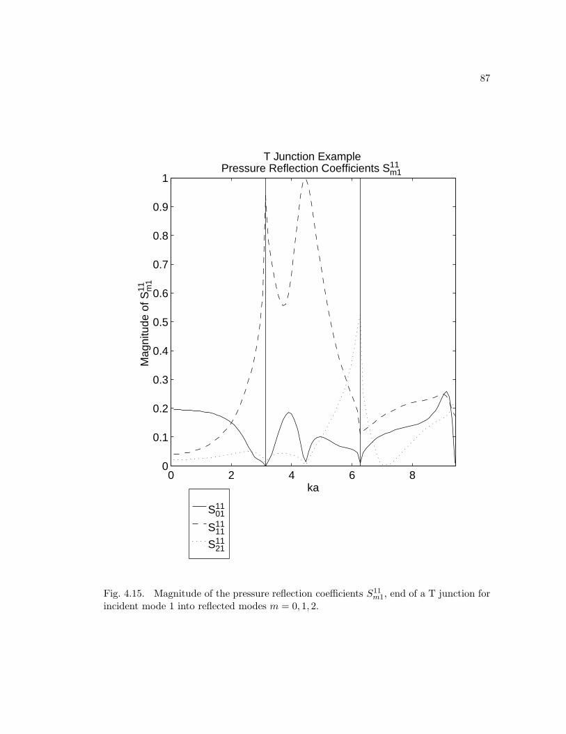
87
S1101
S1111
S1121
0 2 4 6 80
0.1
0.2
0.3
0.4
0.5
0.6
0.7
0.8
0.9
1
ka
Pressure Reflection Coefficients S11m1
T Junction ExampleM
agni
tude
of S
11 m1
Fig. 4.15. Magnitude of the pressure reflection coefficients S11m1, end of a T junction for
incident mode 1 into reflected modes m = 0, 1, 2.
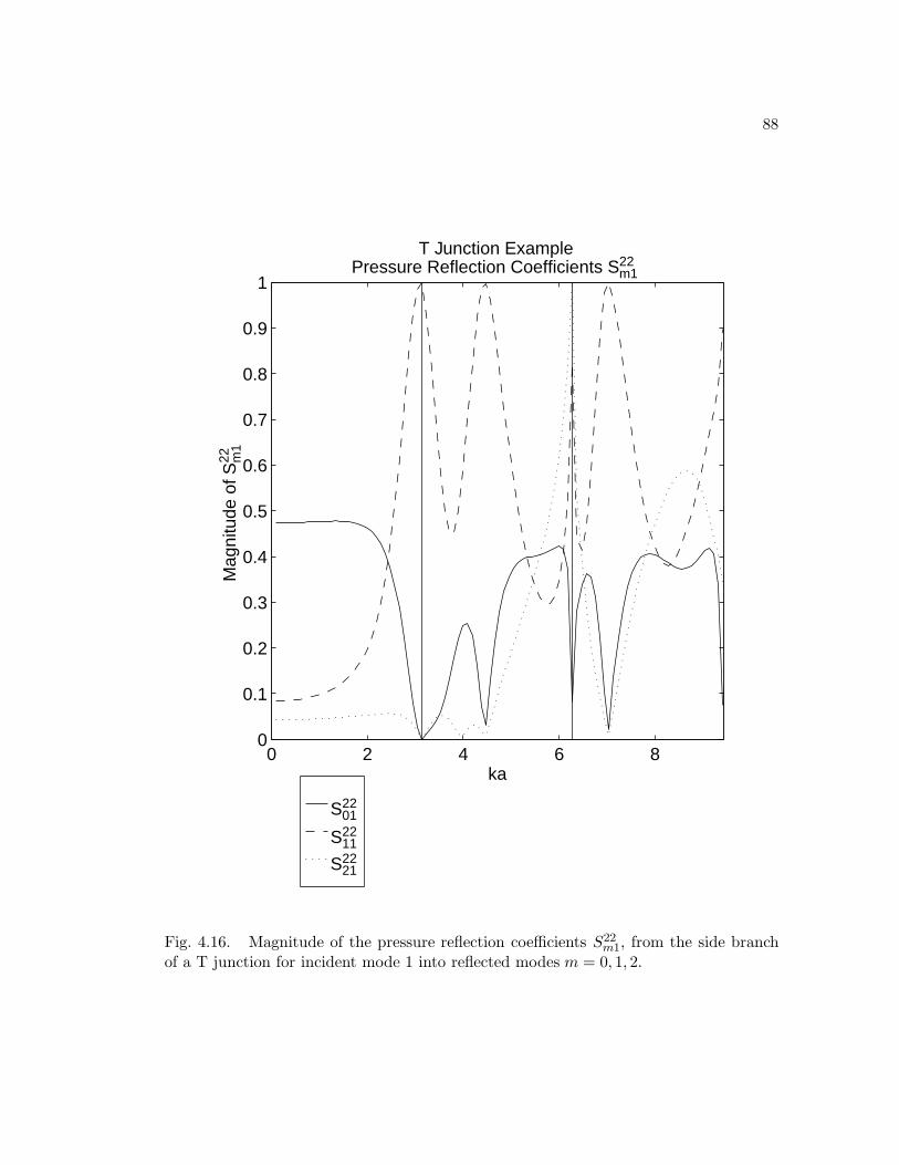
88
S2201
S2211
S2221
0 2 4 6 80
0.1
0.2
0.3
0.4
0.5
0.6
0.7
0.8
0.9
1
ka
Pressure Reflection Coefficients S22m1
T Junction ExampleM
agni
tude
of S
22 m1
Fig. 4.16. Magnitude of the pressure reflection coefficients S22m1, from the side branch
of a T junction for incident mode 1 into reflected modes m = 0, 1, 2.
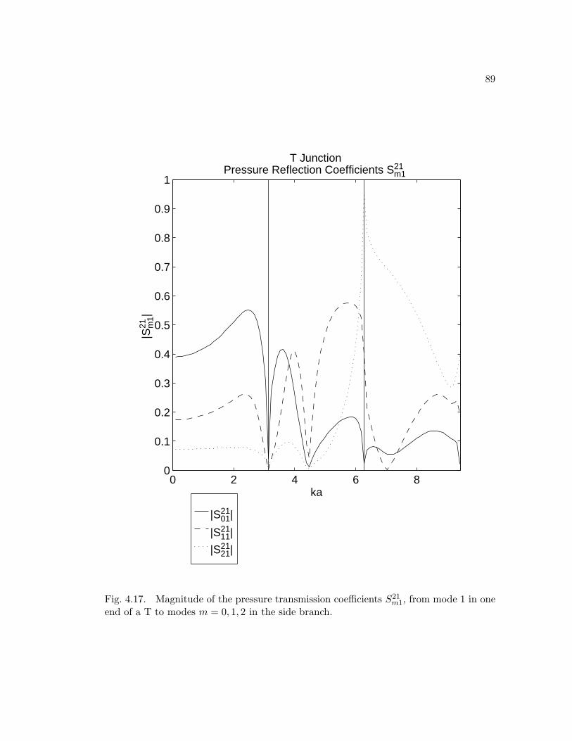
89
|S2101|
|S2111|
|S2121|
0 2 4 6 80
0.1
0.2
0.3
0.4
0.5
0.6
0.7
0.8
0.9
1
ka
Pressure Reflection Coefficients S21m1
T Junction|S
21 m1|
Fig. 4.17. Magnitude of the pressure transmission coefficients S21m1, from mode 1 in one
end of a T to modes m = 0, 1, 2 in the side branch.
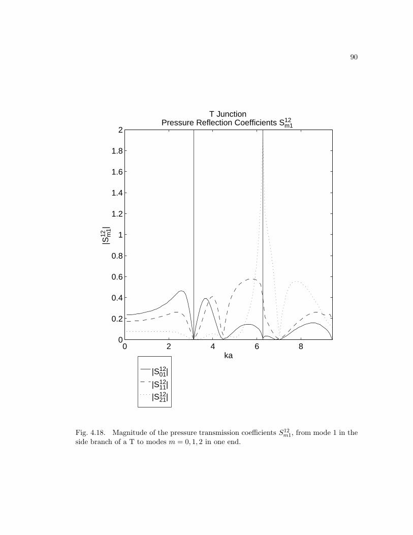
90
|S1201|
|S1211|
|S1221|
0 2 4 6 80
0.2
0.4
0.6
0.8
1
1.2
1.4
1.6
1.8
2
ka
Pressure Reflection Coefficients S12m1
T Junction|S
12 m1|
Fig. 4.18. Magnitude of the pressure transmission coefficients S12m1, from mode 1 in the
side branch of a T to modes m = 0, 1, 2 in one end.

91
|S1301|
|S1311|
|S1321|
0 2 4 6 80
0.1
0.2
0.3
0.4
0.5
0.6
0.7
0.8
0.9
1
ka
Pressure Reflection Coefficients S13m1
T Junction|S
13 m1|
Fig. 4.19. Magnitude of the pressure transmission coefficients S13m1, from mode 1 in one
end of a T to modes m = 0, 1, 2 in the other end.

92
S1102
S1112
S1122
0 2 4 6 80
0.1
0.2
0.3
0.4
0.5
0.6
0.7
0.8
0.9
1
ka
Pressure Reflection Coefficients S11m2
T Junction ExampleM
agni
tude
of S
11 m2
Fig. 4.20. Magnitude of the pressure reflection coefficients, S11m2, from of one end of a
T junction for incident mode 2 into reflected modes m = 0, 1, 2.
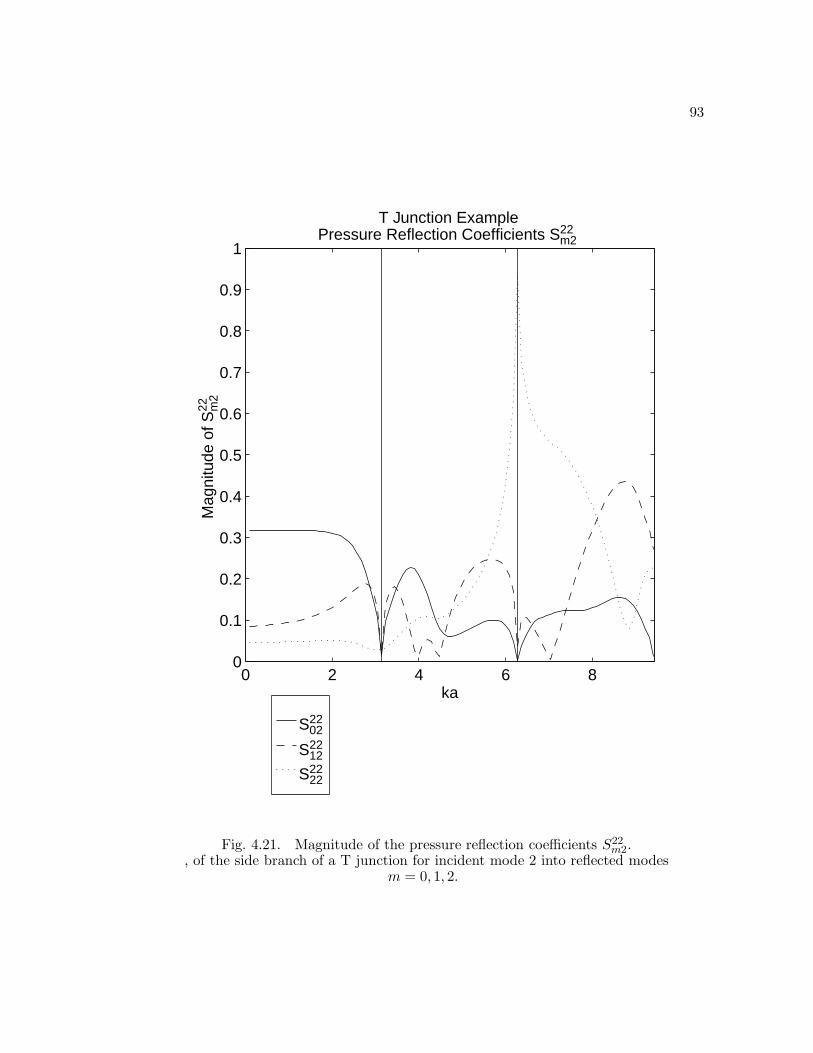
93
S2202
S2212
S2222
0 2 4 6 80
0.1
0.2
0.3
0.4
0.5
0.6
0.7
0.8
0.9
1
ka
Pressure Reflection Coefficients S22m2
T Junction ExampleM
agni
tude
of S
22 m2
Fig. 4.21. Magnitude of the pressure reflection coefficients S22m2.
, of the side branch of a T junction for incident mode 2 into reflected modesm = 0, 1, 2.
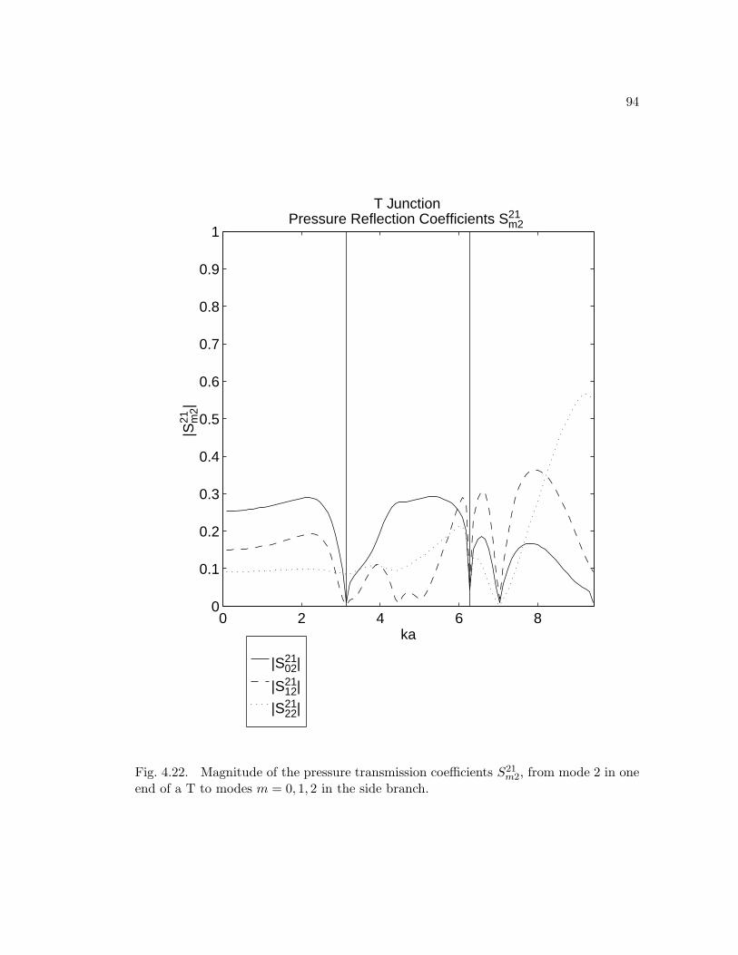
94
|S2102|
|S2112|
|S2122|
0 2 4 6 80
0.1
0.2
0.3
0.4
0.5
0.6
0.7
0.8
0.9
1
ka
Pressure Reflection Coefficients S21m2
T Junction|S
21 m2|
Fig. 4.22. Magnitude of the pressure transmission coefficients S21m2, from mode 2 in one
end of a T to modes m = 0, 1, 2 in the side branch.
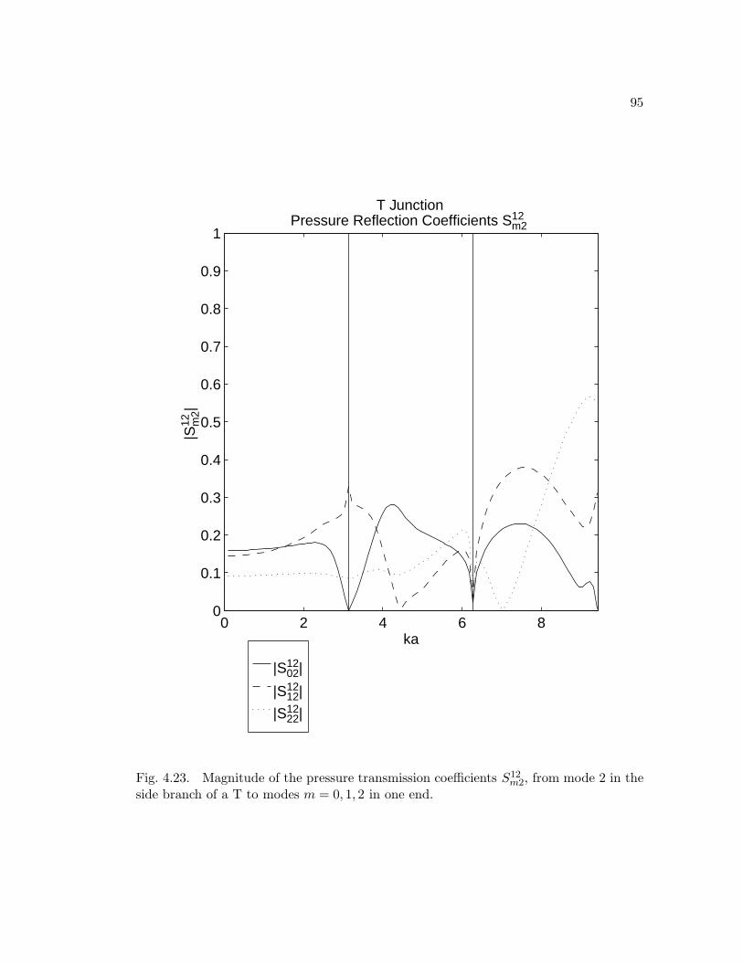
95
|S1202|
|S1212|
|S1222|
0 2 4 6 80
0.1
0.2
0.3
0.4
0.5
0.6
0.7
0.8
0.9
1
ka
Pressure Reflection Coefficients S12m2
T Junction|S
12 m2|
Fig. 4.23. Magnitude of the pressure transmission coefficients S12m2, from mode 2 in the
side branch of a T to modes m = 0, 1, 2 in one end.

96
|S1302|
|S1312|
|S1322|
0 2 4 6 80
0.1
0.2
0.3
0.4
0.5
0.6
0.7
0.8
0.9
1
ka
Pressure Reflection Coefficients S13m2
T Junction|S
13 m2|
Fig. 4.24. Magnitude of the pressure transmission coefficients S13m2, from mode 2 in one
end of a T to modes m = 0, 1, 2 in the other end.

97
Chapter 5
Modal Scattering and Radiation at an Infinite Baffle
This chapter will develop expressions for the reflection coefficients at the end of
a baffled duct and discuss the characteristics of the radiated pressure.
5.1 General Derivation of Radiation Impedance
Calculating the reflection coefficients at the end of a finite rectangular waveguide is
a difficult, but important problem. Once the reflection coefficients are known, the velocity
at the end of the duct is known, and the radiation from the duct can be computed. With
a known velocity distribution, radiation from the end of a rectangular duct is very similar
to radiation from a baffled rectangular plate. Since the radiation characteristics of baffled
plates are known, the radiation characteristics of the baffled duct are known as well.
There are two basic approaches to determining the radiation of a vibrating re-
gion: use of the Kirchoff-Helmholtz integral theorem (direct integration of the differen-
tial equation) and wavenumber transform techniques. The solution that follows uses the
Kirchoff-Helmholtz integral theorem in the form of the Rayleigh integral.
To solve the duct radiation problem, assume a semi-infinite duct terminating in
an infinite baffle at the plane z = 0 as shown in figure 5.1. In the duct (for z < 0) the
pressure and velocity in the z direction can be expressed as modal expansions. Using
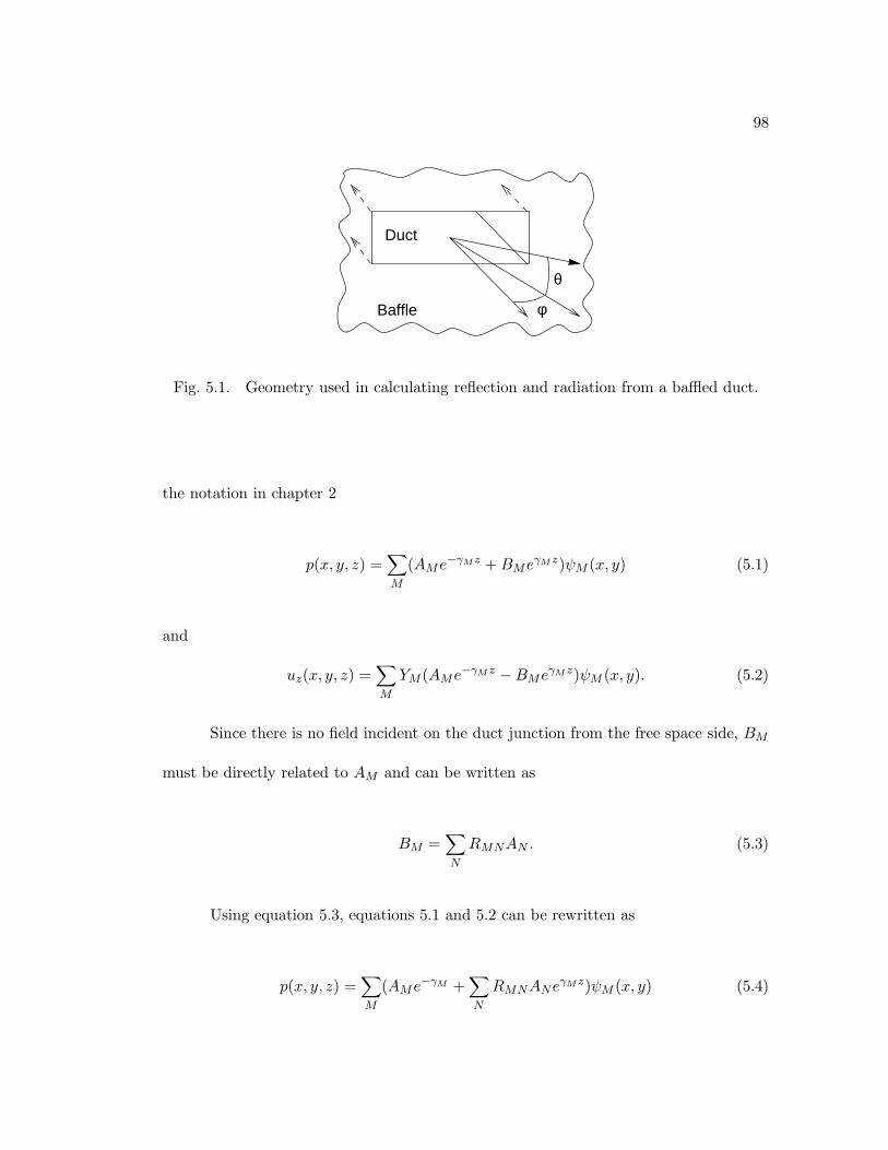
98
φ
θ
Baffle
Duct
Fig. 5.1. Geometry used in calculating reflection and radiation from a baffled duct.
the notation in chapter 2
p(x, y, z) =∑M
(AMe−γMz +BMeγM z)ψM (x, y) (5.1)
and
uz(x, y, z) =∑M
YM (AMe−γM z −BMeγM z)ψM (x, y). (5.2)
Since there is no field incident on the duct junction from the free space side, BM
must be directly related to AM and can be written as
BM =∑N
RMNAN . (5.3)
Using equation 5.3, equations 5.1 and 5.2 can be rewritten as
p(x, y, z) =∑M
(AMe−γM +∑N
RMNANeγM z)ψM (x, y) (5.4)

99
and
uz(x, y, z) =∑M
YM (AMe−γM z −∑N
RMNANeγM z)ψM (x, y). (5.5)
For a baffled duct, the velocity on the baffle is zero and the pressure can be
determined by using the Rayleigh integral as described in chapter 2. Using the Green’s
function for a baffled radiator, and given the normal velocity uz at z = 0, the pressure
outside the duct will be
p(x, y, z) =jkρc
2π
∫∫S
uz(x0, y0)e−jkr
rdS (5.6)
where r =√
(x− x0)2 + (y − y0)2 + z2 and S is the area of the duct.
At the baffle, the pressure p and normal velocity uz are continuous across the
interface. Inserting equations 5.4 and 5.5 into equation 5.6 yields
∑M
(AM +∑N
RMNAN )ψM (x, y) =jkρc
2π
∑M
YM (AM −∑N
RMNAN )
×a∫
0
b∫0
ψM (x0, y0)e−jkr
rdx0dy0 (5.7)
where
r =√
(x− x0)2 + (y − y0)2. (5.8)
Multiplying equation 5.7 by ψR and integrating across the duct cross section will
eliminate the sum on the left hand side of the equation because of orthogonality of the
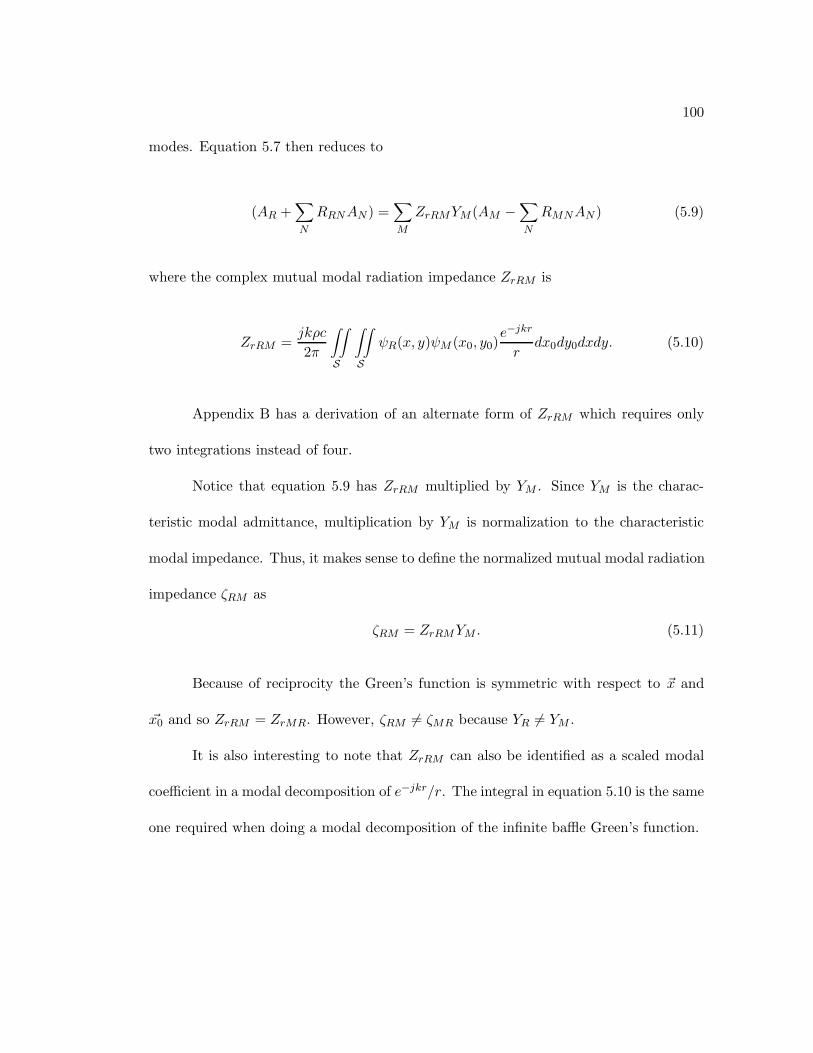
100
modes. Equation 5.7 then reduces to
(AR +∑N
RRNAN ) =∑M
ZrRMYM (AM −∑N
RMNAN ) (5.9)
where the complex mutual modal radiation impedance ZrRM is
ZrRM =jkρc
2π
∫∫S
∫∫S
ψR(x, y)ψM (x0, y0)e−jkr
rdx0dy0dxdy. (5.10)
Appendix B has a derivation of an alternate form of ZrRM which requires only
two integrations instead of four.
Notice that equation 5.9 has ZrRM multiplied by YM . Since YM is the charac-
teristic modal admittance, multiplication by YM is normalization to the characteristic
modal impedance. Thus, it makes sense to define the normalized mutual modal radiation
impedance ζRM as
ζRM = ZrRMYM . (5.11)
Because of reciprocity the Green’s function is symmetric with respect to ~x and
~x0 and so ZrRM = ZrMR. However, ζRM 6= ζMR because YR 6= YM .
It is also interesting to note that ZrRM can also be identified as a scaled modal
coefficient in a modal decomposition of e−jkr/r. The integral in equation 5.10 is the same
one required when doing a modal decomposition of the infinite baffle Green’s function.
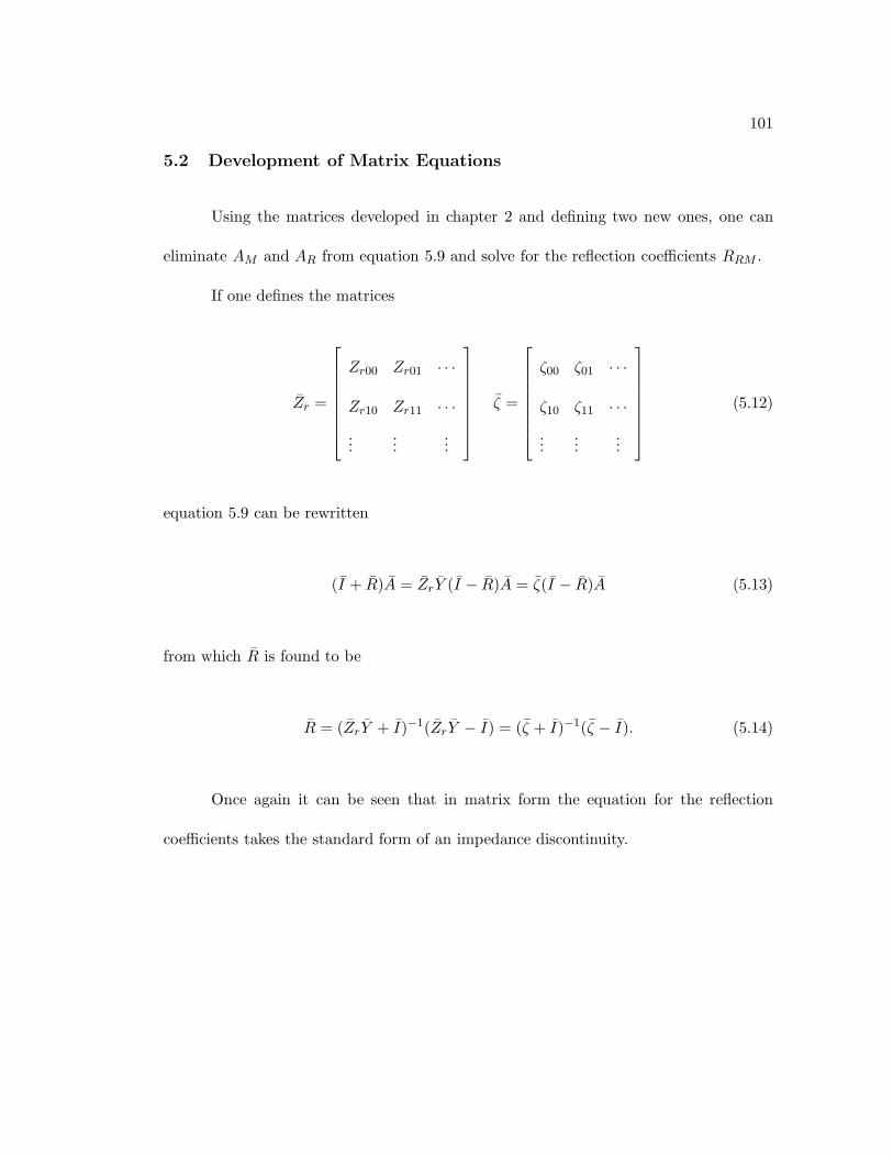
101
5.2 Development of Matrix Equations
Using the matrices developed in chapter 2 and defining two new ones, one can
eliminate AM and AR from equation 5.9 and solve for the reflection coefficients RRM .
If one defines the matrices
Zr =
Zr00 Zr01 · · ·
Zr10 Zr11 · · ·...
......
ζ =
ζ00 ζ01 · · ·
ζ10 ζ11 · · ·...
......
(5.12)
equation 5.9 can be rewritten
(I + R)A = ZrY (I − R)A = ζ(I − R)A (5.13)
from which R is found to be
R = (ZrY + I)−1(ZrY − I) = (ζ + I)−1(ζ − I). (5.14)
Once again it can be seen that in matrix form the equation for the reflection
coefficients takes the standard form of an impedance discontinuity.
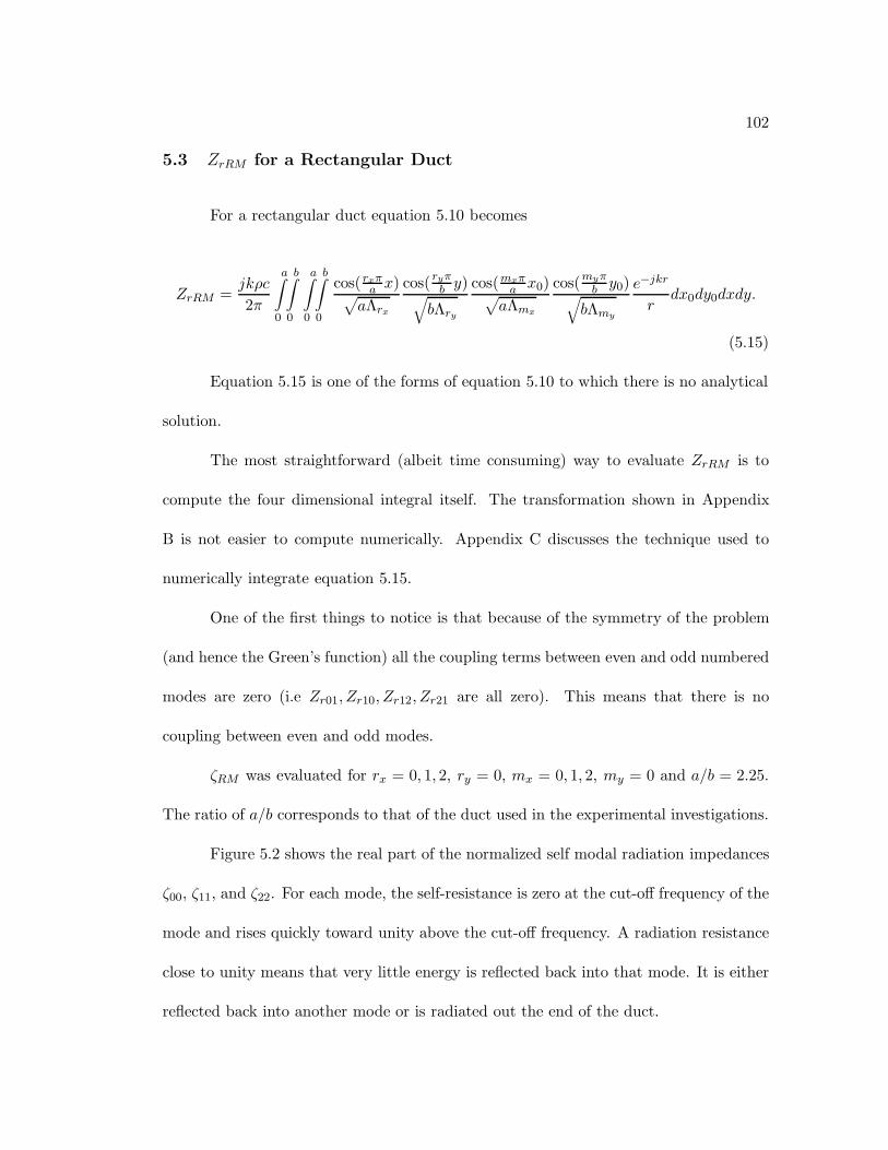
102
5.3 ZrRM for a Rectangular Duct
For a rectangular duct equation 5.10 becomes
ZrRM =jkρc
2π
a∫0
b∫0
a∫0
b∫0
cos( rxπa x)√aΛrx
cos( ryπb y)√bΛry
cos(mxπa x0)√aΛmx
cos(myπb y0)√bΛmy
e−jkr
rdx0dy0dxdy.
(5.15)
Equation 5.15 is one of the forms of equation 5.10 to which there is no analytical
solution.
The most straightforward (albeit time consuming) way to evaluate ZrRM is to
compute the four dimensional integral itself. The transformation shown in Appendix
B is not easier to compute numerically. Appendix C discusses the technique used to
numerically integrate equation 5.15.
One of the first things to notice is that because of the symmetry of the problem
(and hence the Green’s function) all the coupling terms between even and odd numbered
modes are zero (i.e Zr01, Zr10, Zr12, Zr21 are all zero). This means that there is no
coupling between even and odd modes.
ζRM was evaluated for rx = 0, 1, 2, ry = 0, mx = 0, 1, 2, my = 0 and a/b = 2.25.
The ratio of a/b corresponds to that of the duct used in the experimental investigations.
Figure 5.2 shows the real part of the normalized self modal radiation impedances
ζ00, ζ11, and ζ22. For each mode, the self-resistance is zero at the cut-off frequency of the
mode and rises quickly toward unity above the cut-off frequency. A radiation resistance
close to unity means that very little energy is reflected back into that mode. It is either
reflected back into another mode or is radiated out the end of the duct.

103
Figure 5.3 shows the imaginary part of the normalized self modal radiation impedances
ζ00, ζ11, and ζ22. For each mode, the self reactance is zero at the cut-off frequency, quickly
rises to a value near 0.5 close to the cut-off frequency of the next mode and then drops
back toward zero at higher frequencies. Below the cut-off frequency the reactance is
small, but only values above the cut-off frequency are significant since only modes above
their cut-off frequency propagate energy toward the end of the duct. The radiation
reactance is a measure of the energy stored in the near field of the end of the duct.
Figure 5.5 shows the real part of the mutual modal radiation impedances ζ20 and
ζ02. The mutual resistance for the (02) mode is positive below the cut-off frequency and
negative above. The mutual resistance for the (20) mode is negative for all frequencies.
Figure 5.5 shows the imaginary part of the mutual modal radiation impedance ζ20
and ζ02. The mutual reactance for the (02) mode and the (20) mode are similar, negative
below the cut-off frequency and positive above the cut-off frequency of the second mode.
While the physical interpretation of these values is not clear, it is clear that the
(02) coupling is different from the (20) coupling. Because the impedances are non-zero
it is also clear that both propagating energy and evanescent energy (energy stored in the
near field) are being exchanged between the modes. Since the amplitudes of the mutual
radiation impedance are not negligible compared to the self radiation impedances, modal
coupling at the end of the duct should not be ignored at frequencies near or above the
cut-off frequency of the mode.
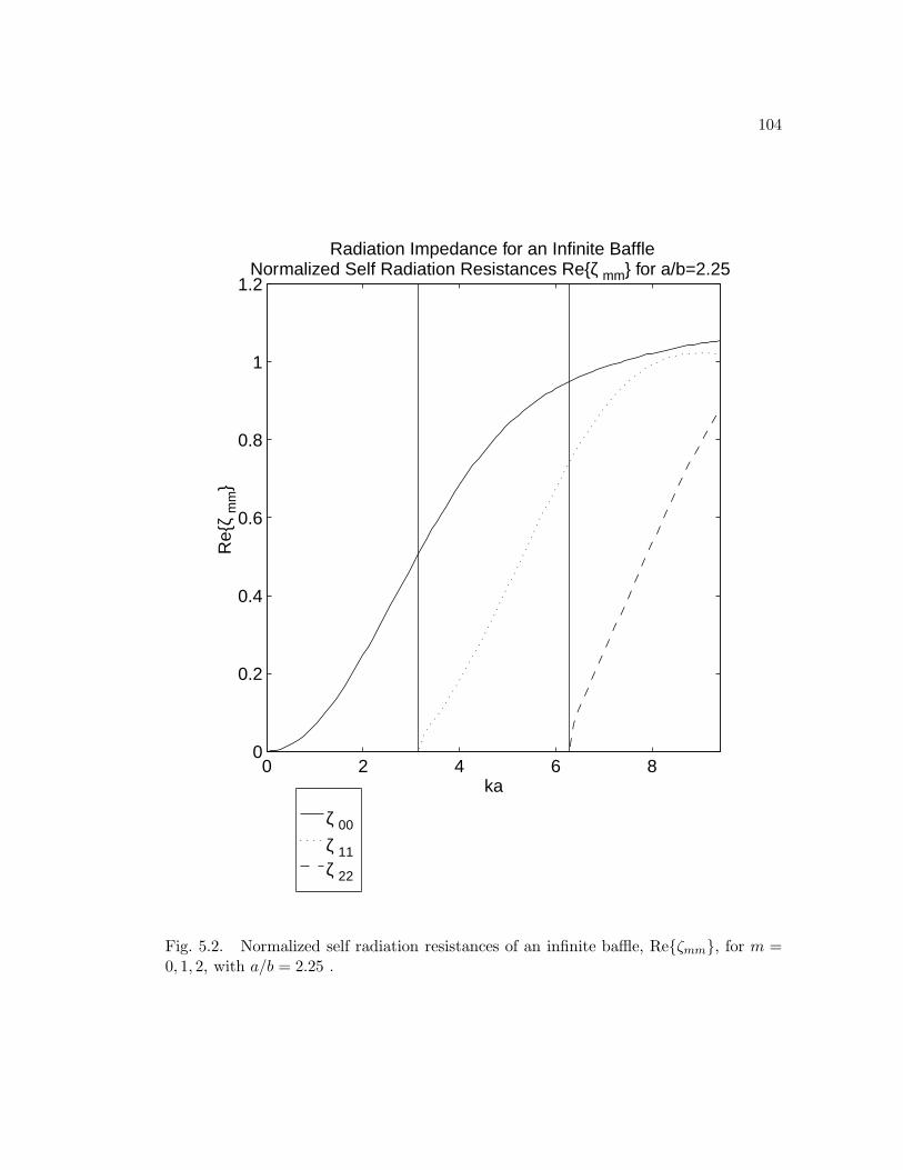
104
ζ 00
ζ 11ζ 22
0 2 4 6 80
0.2
0.4
0.6
0.8
1
1.2
ka
Normalized Self Radiation Resistances Re{ζ mm} for a/b=2.25Radiation Impedance for an Infinite Baffle
Re{
ζ m
m}
Fig. 5.2. Normalized self radiation resistances of an infinite baffle, Re{ζmm}, for m =0, 1, 2, with a/b = 2.25 .

105
ζ 00
ζ 11ζ 22
0 2 4 6 80
0.1
0.2
0.3
0.4
0.5
0.6
0.7
ka
Normalized Self Radiation Reactance Im{ζ mm} for a/b=2.25Radiation Impedance for an Infinite Baffle
Im{ζ
mm
}
Fig. 5.3. Normalized self radiation reactances of an infinite baffle, Im{ζmm}, for m =0, 1, 2 with a/b = 2.25.

106
ζ 02ζ 20
0 2 4 6 8−0.3
−0.25
−0.2
−0.15
−0.1
−0.05
0
0.05
0.1
0.15
0.2
ka
Normalized Mutual Radiation Resistance Re{ζ rm} for a/b=2.25Radiation Impedance for an Infinite Baffle
Re{
ζ rm
}
Fig. 5.4. Normalized mutual radiation resistances of an infinite baffle, Re{ζrm} andIm{ζrm}, for m = 0, 1, 2 with a/b = 2.25.

107
ζ 02ζ 20
0 2 4 6 8−0.2
−0.15
−0.1
−0.05
0
0.05
0.1
0.15
0.2
ka
Normalized Mutual Radiation Reactance Im{ζ rm} for a/b=2.25Radiation Impedance for an Infinite Baffle
Im{ζ
rm
}
Fig. 5.5. Normalized mutual radiation reactances of an infinite baffle, Re{ζrm} andIm{ζrm}, for m = 0, 1, 2 with a/b = 2.25.
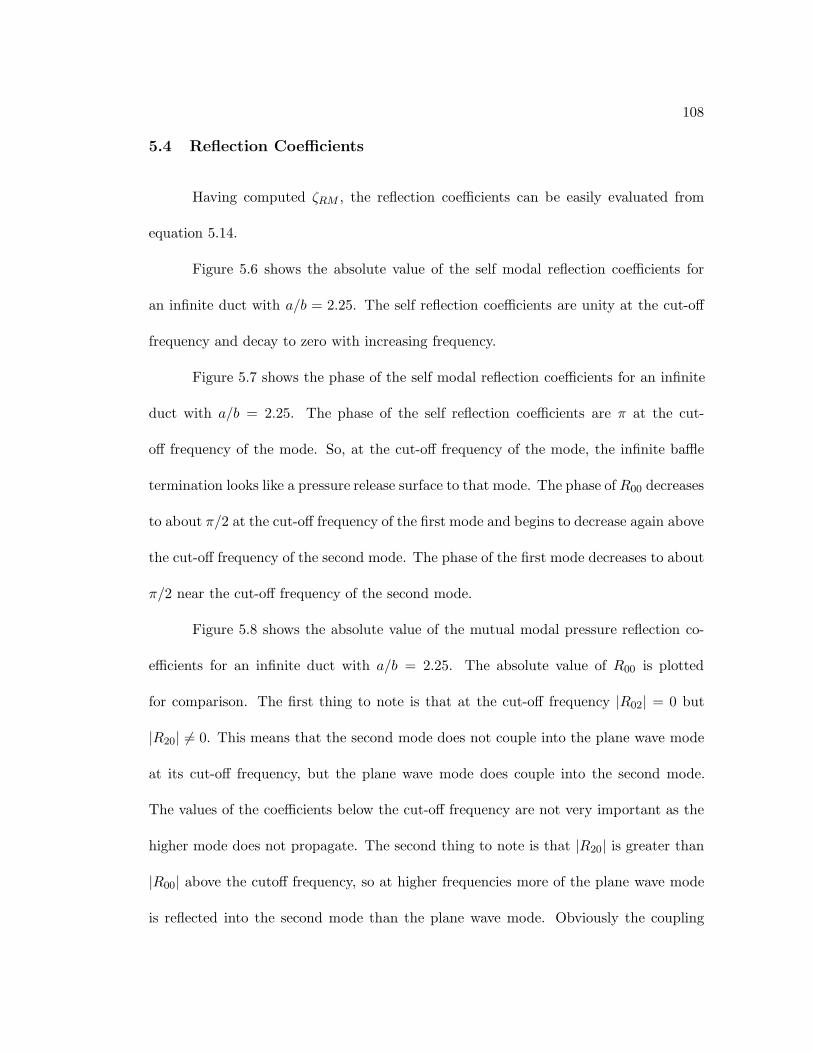
108
5.4 Reflection Coefficients
Having computed ζRM , the reflection coefficients can be easily evaluated from
equation 5.14.
Figure 5.6 shows the absolute value of the self modal reflection coefficients for
an infinite duct with a/b = 2.25. The self reflection coefficients are unity at the cut-off
frequency and decay to zero with increasing frequency.
Figure 5.7 shows the phase of the self modal reflection coefficients for an infinite
duct with a/b = 2.25. The phase of the self reflection coefficients are π at the cut-
off frequency of the mode. So, at the cut-off frequency of the mode, the infinite baffle
termination looks like a pressure release surface to that mode. The phase of R00 decreases
to about π/2 at the cut-off frequency of the first mode and begins to decrease again above
the cut-off frequency of the second mode. The phase of the first mode decreases to about
π/2 near the cut-off frequency of the second mode.
Figure 5.8 shows the absolute value of the mutual modal pressure reflection co-
efficients for an infinite duct with a/b = 2.25. The absolute value of R00 is plotted
for comparison. The first thing to note is that at the cut-off frequency |R02| = 0 but
|R20| 6= 0. This means that the second mode does not couple into the plane wave mode
at its cut-off frequency, but the plane wave mode does couple into the second mode.
The values of the coefficients below the cut-off frequency are not very important as the
higher mode does not propagate. The second thing to note is that |R20| is greater than
|R00| above the cutoff frequency, so at higher frequencies more of the plane wave mode
is reflected into the second mode than the plane wave mode. Obviously the coupling

109
effects of the plane wave mode into propagating higher order modes are not negligible in
any way.
Figure 5.9 shows the phase of the mutual modal pressure reflection coefficients
for an infinite duct with a/b = 2.25. The phase of R02 and R20 differ by π/2 until the
cut-off frequency of the mode when it begins to decrease. Above the cut-off frequency
of the second mode the phase of the two is the same.
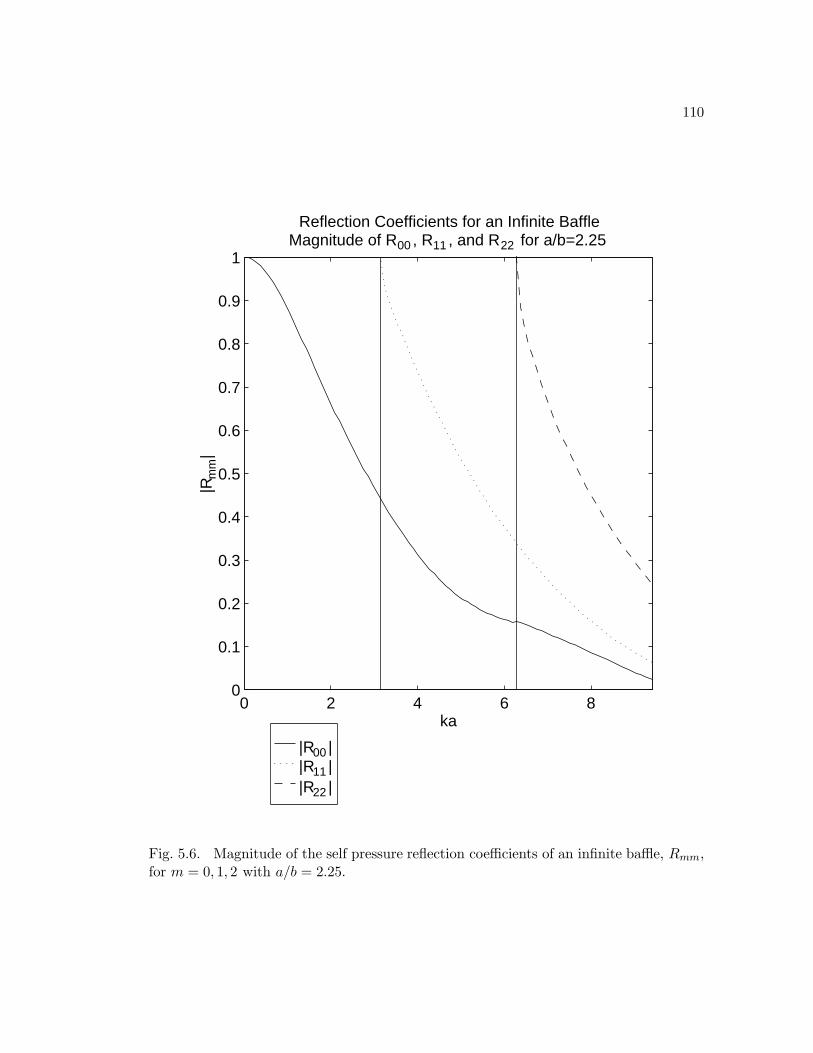
110
|R00 ||R11 ||R22 |
0 2 4 6 80
0.1
0.2
0.3
0.4
0.5
0.6
0.7
0.8
0.9
1
ka
Magnitude of R00 , R11 , and R22 for a/b=2.25Reflection Coefficients for an Infinite Baffle
|Rm
m|
Fig. 5.6. Magnitude of the self pressure reflection coefficients of an infinite baffle, Rmm,for m = 0, 1, 2 with a/b = 2.25.

111
Phase of R00Phase of R11Phase of R22
0 2 4 6 80
0.5
1
1.5
2
2.5
3
ka
Phase of R00 , R11 , and R22 for a/b=2.25Reflection Coefficients for an Infinite Baffle
Pha
se o
f Rrm
Fig. 5.7. Phase of the self pressure reflection coefficients of an infinite baffle, Rmm, form = 0, 1, 2 with a/b = 2.25.

112
|R00 ||R02 ||R20 |
0 2 4 6 80
0.1
0.2
0.3
0.4
0.5
0.6
0.7
0.8
0.9
1
ka
Magnitude of R00 , R02 , R20 for a/b=2.25Reflection Coefficients for an Infinite Baffle
|Rrm
|
Fig. 5.8. Magnitude of the mutual pressure reflection coefficients R02 and R20 of aninfinite baffle for m = 0, 1, 2, with a/b = 2.25. |R00| is shown for comparison.

113
Phase of R00Phase of R02Phase of R20
0 2 4 6 8−3
−2
−1
0
1
2
3
ka
Phase of R00 , R20 , and R02 for a/b=2.25Reflection Coefficients for an Infinite Baffle
Pha
se o
f Rrm
Fig. 5.9. Phase of the mutual reflection coefficients R02 and R20 of an infinite baffle form = 0, 1, 2, with a/b = 2.25. The phase of R00 is shown for comparison.
114
5.5 Radiation
5.5.1 Directivity
Having determined the reflection coefficients RRM , the velocity at the interface
is completely determined. Given the velocity distribution, the pressure at any point
outside the duct can be determined by use of the Rayleigh integral.
The pressure directivity and the radiated power of each particular mode are very
useful in determining the radiation outside the duct given a mode incident at the end of
the duct.
The velocity at the end of the duct is
uz =∑M
YM (AM −∑N
RMNAN )φM . (5.16)
The pressure outside the duct, for any position ~R is given by the Rayleigh integral
p(x, y, z) =γM2π
∑M
YM(AM −∑N
RMNAN )∫∫S0
ψM (x0, y0)ejkR
Rdx0dy0. (5.17)
where R =√
(x− x0)2 + (y − y0)2 + z2.
Even if only one mode is incident, there can be many modes reflected, so regard-
less of the incident wave there is a superposition of many modes. However, to better
understand the physics of the problem one can consider the radiation of a single mode.
115
The pressure will then have the form
pM (x, y, z) = CM
∫∫S0
ψM (x0, y0)ejkR
Rdx0dy0. (5.18)
where CM = jkρc/(2π)YMAM (1−RMM ) is the total modal amplitude of the mode M.
To determine the directivity pattern and radiated power, the pressure can be
evaluated in the far field. The standard far field approximation is
R ≈ r − x sin(θ) cos(φ)− y sin(θ) sin(φ) (5.19)
where
r =√x2 + y2 + z2. (5.20)
With this approximation equation 5.18 becomes
pM (x, y, z) = CMejkr
r
∫∫S0
ψ(x0, y0)e−j(xα+yβ)dx0dy0 (5.21)
where α = k sin(θ) cos(φ) and β = k sin(θ) sin(φ).
The integral can be recognized as a wavenumber transform of ψ (see appendix B)
by replacing α and β with kx and ky. The far field equation can be then be written
pM(r, φ, θ) = CMejkr
rΨM (α, β). (5.22)

116
For the purposes of this thesis, the directivity DM (φ, θ) is defined as the ratio
of the magnitude of ΨM (α, β) divided by the maximum value of ΨM (α, β). With this
definition DM (φ, θ) contains the angular dependence of pM .
Figure 5.10 shows the directivity for the plane wave mode with ka = 0.5π, 1.5π,
2.5π, and 3.5π. Recall that the first higher order mode cut-off is at ka = π. Below the
cut-off frequency of the first mode the radiation is pretty much omni-directional. Just
above the cut-off frequency of the first mode beaming effects are clearly apparent. Above
the cut-off frequency of the second mode lobing has begun.
Figure 5.11 shows the directivity for the first horizontal mode with ka = 0.5π,
1.5π, 2.5π, and 3.5π. In contrast to the plane wave mode, there is no radiation on axis;
the radiation is beamed far off to the sides. Below the cut-off frequency for the mode the
direction of maximum radiation is at ±90o. At higher frequencies the radiation beams
narrow and get closer to the axis. Secondary lobes are apparent above cut-off frequency
of the third mode.
Figure 5.12 shows the directivity for the second horizontal mode with ka = 0.5π,
1.5π, 2.5π, 3.5π. Again, below the cut-off frequency of the mode the radiation maximum
is at ±90o. Again, above cut-off frequency of the mode the beams are directed more
toward the main axis.
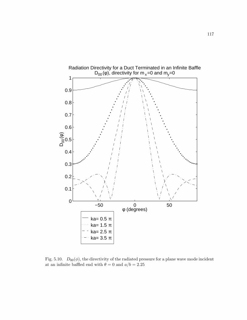
117
ka= 0.5 π ka= 1.5 π ka= 2.5 π ka= 3.5 π
−50 0 500
0.1
0.2
0.3
0.4
0.5
0.6
0.7
0.8
0.9
1D00 (φ ), directivity for m x=0 and my=0
Radiation Directivity for a Duct Terminated in an Infinite Baffle
φ (degrees)
D00
(φ)
Fig. 5.10. D00(φ), the directivity of the radiated pressure for a plane wave mode incidentat an infinite baffled end with θ = 0 and a/b = 2.25
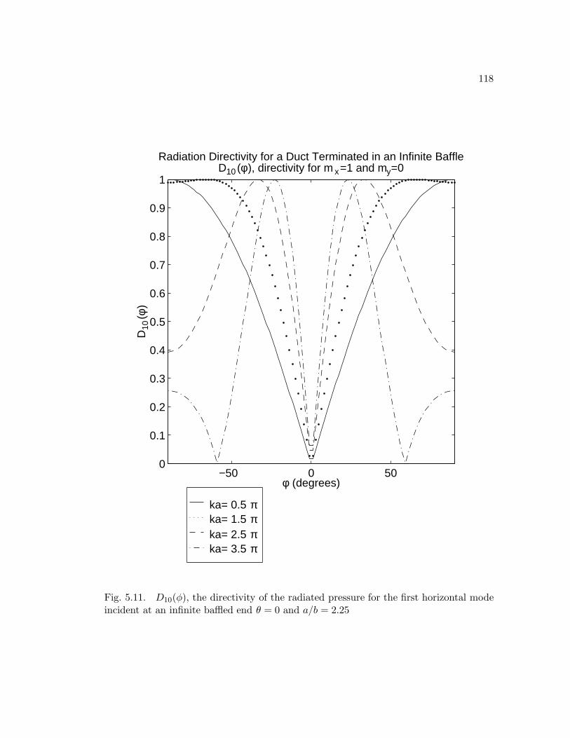
118
ka= 0.5 π ka= 1.5 π ka= 2.5 π ka= 3.5 π
−50 0 500
0.1
0.2
0.3
0.4
0.5
0.6
0.7
0.8
0.9
1D10 (φ ), directivity for m x=1 and my=0
φ (degrees)
D10
(φ)
Radiation Directivity for a Duct Terminated in an Infinite Baffle
Fig. 5.11. D10(φ), the directivity of the radiated pressure for the first horizontal modeincident at an infinite baffled end θ = 0 and a/b = 2.25

119
ka= 0.5 π ka= 1.5 π ka= 2.5 π ka= 3.5 π
−50 0 500
0.1
0.2
0.3
0.4
0.5
0.6
0.7
0.8
0.9
1D20 (φ ), directivity for m x=2 and my=0
φ (degrees)
D20
(φ)
Radiation Directivity for a Duct Terminated in an Infinite Baffle
Fig. 5.12. D20(φ), the directivity of the radiated pressure for the second horizontalmode wave mode incident at an infinite baffled end with θ = 0 and a/b = 2.25

120
5.5.2 Radiated Power
The radiated power can be obtained by several methods. The power could be
obtained by integrating the square of the far field pressure. As with radiation from
rectangular panels [66], this would lead to more integrals which must be approximated or
numerically evaluated. Alternatively, one could use the knowledge of the duct reflection
coefficients to compute the radiated power.
The power in a single traveling mode of amplitude AM is
ΠM =kM
2kρc|AM |2. (5.23)
From this the total power traveling toward the duct end is
Π+ =∑M
kM2kρc
|AM |2 = AH Y A (5.24)
where H denotes the hermitian operator which is the complex conjugate transpose.
The total power reflected back from the end of the duct is
Π− = BH Y B = (RA)H Y RA = AHRH Y RA. (5.25)
The difference between the incident and the reflected powers must be the radiated
power because there are no losses. Thus the total radiated power is
ΠRad = AH(Y − RH Y R)A. (5.26)
121
Chapter 6
Experimental Results
This chapter will discuss the experimental measurements of the reflection coeffi-
cients of a baffled duct.
6.1 Modal Decomposition
In order to measure reflection coefficients, one must first determine the modal
amplitudes AM and BM in the duct. Experimentally this is done by measuring the
pressure at a number of discrete positions and determining AM and BM from those
measurements.
In chapter 2 it was shown that the pressure could be written
p(x, y, z) =∑M
(AMe−γM z +BMeγM z)ψM (x, y). (6.1)
Defining the modal pressure as
PM (z) = (AMe−γM z +BMeγM z) (6.2)
equation 6.1 can be rewritten in terms of modal pressures
p(x, y, z) =∑M
PM (z)ψM (x, y). (6.3)
122
This equation shows that the pressure can be broken into a modal component
which is z dependent and an eigenfunction which is x and y dependent.
Defining the matrices
p =
p(x1, y1, z1) p(x1, y1, z2) · · ·
p(x2, y2, z1) p(x2, y2, z2) · · ·...
.... . .
(6.4)
ψ =
ψ0(x1, y1) ψ1(x1, y1) · · ·
ψ0(x2, y2) ψ1(x2, y2) · · ·...
.... . .
(6.5)
and
PM =
P0(z1) P0(z2) · · ·
P1(z1) P1(z2) · · ·...
.... . .
(6.6)
a collection of pressure measurements can be written as
p = ψPM (6.7)
and the modal pressure can be found from a collection of pressure measurements by the
equation
PM = ψ−1p. (6.8)
123
To be able to uniquely determine PM requires that ψ have a generalized inverse
which means that, among other things, the columns of ψ must be linearly independent.
This limits the x and y positions of the measurements. In addition, to discern N modes
p and ψ must have at least N rows. If they have more than N rows a least squares
solution is obtained.
Once the PbarM are found AM and BM are easily determined.
Defining the matrices
PMZ =
PM (z1)
PM (z2)
...
φM =
e−γM z1 eγM z1
e−γM z2 eγM z2
......
(6.9)
the PM and hence AM and BM can be found since PMZ can be expressed as
PMZ = φ
AM
BM
(6.10)
Then AM and BM can be expressed as
AM
BM
= φ−1M PMZ (6.11)
where φ−1M is the generalized inverse of φM .
124
From equation 6.11 one can see that as a minimum at least measurements at at
least 2 different z positions and N different x, y positions are required to determine AM
and BM for N modes.
6.1.1 Probes vs. Arrays
Since pressures must be measured at several positions the use of microphone ar-
rays or microphone probes immediately suggest themselves. Early experimental work
relied on movable microphone probes for measurements. However, with the advent of
small electret microphones, microphone arrays are now practical for use in modal mea-
surements.
When using a single microphone or microphone probe, the problem of matching
the microphones does not exist since there is only one microphone. However, because
the microphone must be moved to many positions the technique is very time consuming
and fraught with positioning errors.
If an array of microphones is used, positioning problems are either eliminated or
reduced; however, microphone calibration and matching must now be considered. Be-
cause of the complexity of the electronics and calibration, the use of a full two dimensional
array of microphones is also fraught with difficulties.
As a compromise between the microphone probe and two dimensional array, a
linear array of microphones could be used. Either a horizontal array which is traversed
along the duct length or an axial array which is traversed across the duct width could
be used. In either case, there is less positioning error than with the single microphone
125
probe and a considerable speed up of the measurement process, while there is less cal-
ibration and phase matching problems and less electronics complexity than with a full
two dimensional array. For these reasons a linear array was used for the measurements
in this thesis.
6.1.2 Horizontal vs. Axial Arrays
Once a researcher has decided to use linear arrays, she or he must then choose
between a horizontal or axial array configuration. Looking at the phase characteristics
of the measurements in both directions will help determine the limitations of both types
of measurements.
In the axial direction the pressure varies according to the term e−γM z. The phase
in the axial direction is position and frequency dependent. Even small phase errors in
the measurements will lead to poor calculations of A and B.
In the horizontal direction the pressure varies according to the term ψM (x) which
is not frequency dependent and has only a plus or minus phase. Phase errors are less
likely to be a problem in the horizontal direction.
The microphones and electronics have small phase differences from channel to
channel that are difficult to eliminate. If accurate axial placement is easier than accurate
horizontal placement, mounting the microphones in a horizontal array and accurately
positioning it axially should provide a better measurement than an axial array since the
same microphone is used to sample the axial direction, thus eliminating electronic and
microphone phase differences from the axial measurements and only positioning errors
exist.

126
Fig. 6.1. Side mounted speaker configuration
For the duct used in the experimental work of this thesis it was much easier to
accurately position the microphones axially than horizontally, so a horizontal array was
used.
6.2 Modal Generation
Modal generation is a problem which has already been thoroughly researched
[3, 18, 19]. The usual technique is to have a number of sources mounted on the outside
walls of the duct as shown in figure 6.1. The problem with this configuration is that the
amplitude of the modes generated goes as sinc(ka) where a is the radius of the speaker.
Thus at some frequencies a given mode cannot be generated. In contrast, by placing the
sources at the end of the duct as shown in figure 6.2 the modal coupling and generation
is not frequency dependent (assuming the mode is not cut-off).
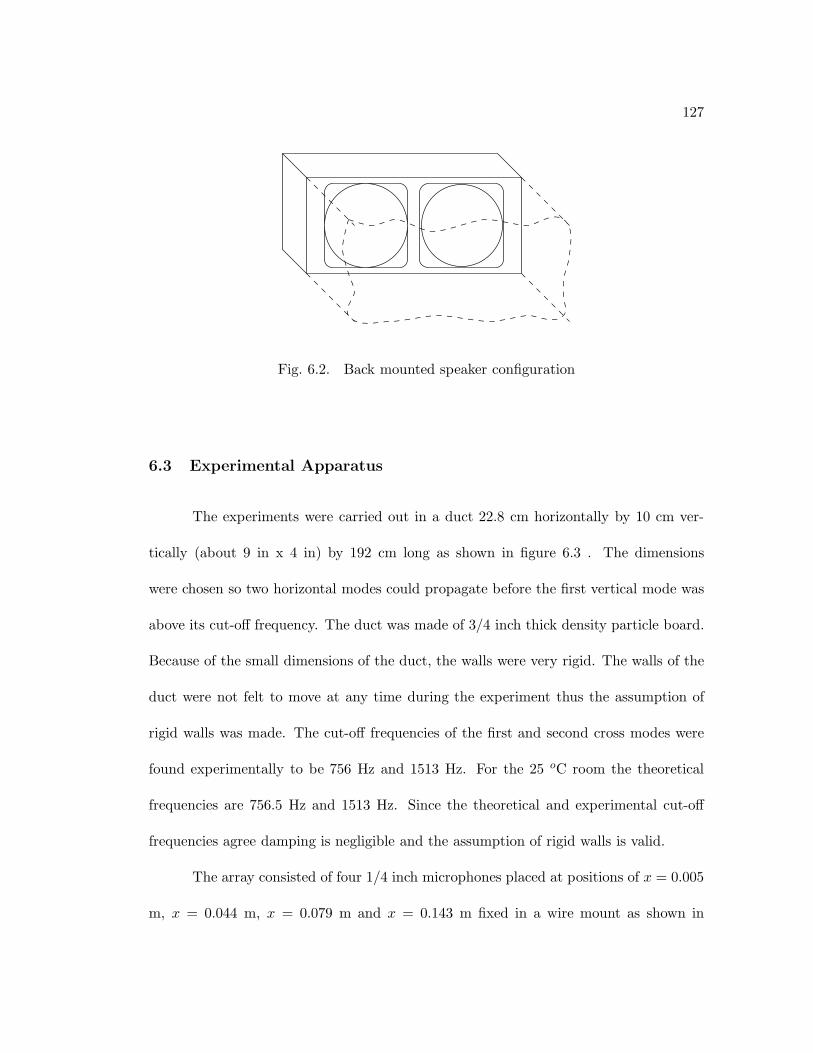
127
Fig. 6.2. Back mounted speaker configuration
6.3 Experimental Apparatus
The experiments were carried out in a duct 22.8 cm horizontally by 10 cm ver-
tically (about 9 in x 4 in) by 192 cm long as shown in figure 6.3 . The dimensions
were chosen so two horizontal modes could propagate before the first vertical mode was
above its cut-off frequency. The duct was made of 3/4 inch thick density particle board.
Because of the small dimensions of the duct, the walls were very rigid. The walls of the
duct were not felt to move at any time during the experiment thus the assumption of
rigid walls was made. The cut-off frequencies of the first and second cross modes were
found experimentally to be 756 Hz and 1513 Hz. For the 25 oC room the theoretical
frequencies are 756.5 Hz and 1513 Hz. Since the theoretical and experimental cut-off
frequencies agree damping is negligible and the assumption of rigid walls is valid.
The array consisted of four 1/4 inch microphones placed at positions of x = 0.005
m, x = 0.044 m, x = 0.079 m and x = 0.143 m fixed in a wire mount as shown in

128
Speakers
Duct is 10 cm high
Moveable Mic Array
22.8 cm Wide
192 cm Long
Fig. 6.3. Duct Setup
figure 6.4. The spacing resulted from attempting to place one microphone as close to
the wall as possible, one microphone at the horizontal midpoint and the other two at
the one third and one fourth points. The small size of the microphones and wire mount
ensured that the acoustic field was disturbed very little by the measurement devices.
The microphones were placed at a vertical height of y = 5 cm, the vertical mid line of
the duct. By placing the microphones at that height, only the vertical plane wave and
odd order modes would be measured - the first vertical mode would not be measured.
The wire mount was attached to a 3/4 in steel tape measure which was used to move
the microphone array and measure its axial position.
The microphones were Panasonic W63AT electret microphones which have a fre-
quency response of ±3 dB from 20 Hz to 20 kHz. A microphone preamplifier with four
identical channels was specially designed for use with the Panasonic electret elements.
The amplifier has level adjustments for each individual microphone. The bias resistors
for the microphones were individually chosen for each microphone element. With optimal
bias resistors, the harmonic distortion was as low as a B&K 4130 reference microphone.
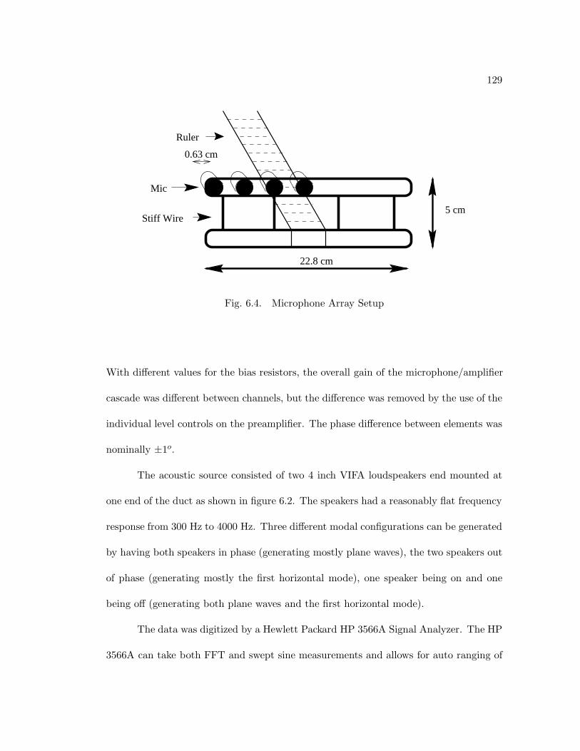
129
Ruler
Mic
Stiff Wire5 cm
22.8 cm
0.63 cm
Fig. 6.4. Microphone Array Setup
With different values for the bias resistors, the overall gain of the microphone/amplifier
cascade was different between channels, but the difference was removed by the use of the
individual level controls on the preamplifier. The phase difference between elements was
nominally ±1o.
The acoustic source consisted of two 4 inch VIFA loudspeakers end mounted at
one end of the duct as shown in figure 6.2. The speakers had a reasonably flat frequency
response from 300 Hz to 4000 Hz. Three different modal configurations can be generated
by having both speakers in phase (generating mostly plane waves), the two speakers out
of phase (generating mostly the first horizontal mode), one speaker being on and one
being off (generating both plane waves and the first horizontal mode).
The data was digitized by a Hewlett Packard HP 3566A Signal Analyzer. The HP
3566A can take both FFT and swept sine measurements and allows for auto ranging of
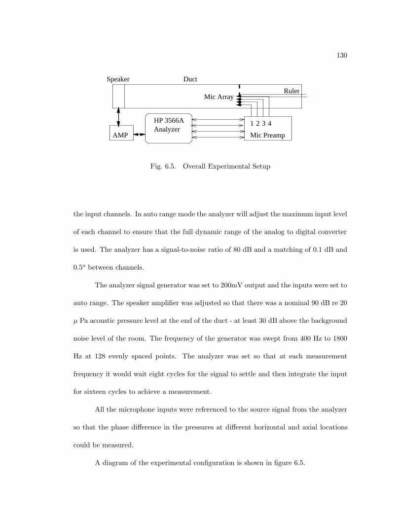
130
Mic Preamp
3 421
AMP
RulerMic Array
HP 3566AAnalyzer
Speaker Duct
Fig. 6.5. Overall Experimental Setup
the input channels. In auto range mode the analyzer will adjust the maximum input level
of each channel to ensure that the full dynamic range of the analog to digital converter
is used. The analyzer has a signal-to-noise ratio of 80 dB and a matching of 0.1 dB and
0.5o between channels.
The analyzer signal generator was set to 200mV output and the inputs were set to
auto range. The speaker amplifier was adjusted so that there was a nominal 90 dB re 20
µ Pa acoustic pressure level at the end of the duct - at least 30 dB above the background
noise level of the room. The frequency of the generator was swept from 400 Hz to 1800
Hz at 128 evenly spaced points. The analyzer was set so that at each measurement
frequency it would wait eight cycles for the signal to settle and then integrate the input
for sixteen cycles to achieve a measurement.
All the microphone inputs were referenced to the source signal from the analyzer
so that the phase difference in the pressures at different horizontal and axial locations
could be measured.
A diagram of the experimental configuration is shown in figure 6.5.
131
6.4 Data Reduction
The data measured by the signal analyzer was stored in HP’s native SDF for-
mat. The data was loaded directly into MATLAB for analysis with a specially written
program.
From the horizontal measurements for each axial position the modal pressures
PM (z) were extracted using equation 6.9. From the modal pressures PM (z), the ampli-
tudes AM and BM were extracted using equation 6.11. Errors were not included in the
decomposition.
6.5 Microphone Calibration and Measurement Caveats
The standard technique for systematic microphone calibration to remove ampli-
tude and phase differences is to expose the microphones to the same field, measure the
amplitude and phase differences and use those differences to correct the measured data.
An alternate method is the “switching” calibration method where the microphones are
physically switched, the measurement redone, and the results are combined in a way
to remove the microphone differences. Because of the number of microphones involved
in this experiment, the “switching” calibration method is not easily employed thus the
other method was used.
To expose the microphones to the same field, the microphones were placed in a
3/8 in thick aluminum plate at the end of a 1M long, 4 in diameter round PVC duct. The
duct was driven by a speaker covering the entire width of the duct at the end opposite
the microphones. It was found that when measuring the frequency response between
132
microphones with a random noise applied to the speaker, the microphone calibration
was not repeatable. If the microphone was removed and replaced in the same position,
the calibration would change by up to ±0.5o at some frequencies. The change was
seemingly random - no systematic change could be found. If the plate was rotated 90o,
the calibration would change up to ±0.5o. If the plate were rotated back, the calibration
would match the previous calibration to within millidegrees. What does this say? First,
the rotation results say it is very difficult to expose the microphones to a uniform field
for calibration purposes. Second, the removal and replacement results say that since
it is so difficult to get the microphones back into the same position that the switching
method of calibration is essentially useless with these microphones.
A similar problem with repeatability showed itself during the measurement pro-
cess. When measuring using random noise and frequency response analysis it was found
that repeated experiments did not give the same results. Repeated trials were found to
differ in phase by as much as 1.5o.
A possible explanation of part of the measurement and calibration problems comes
from Bendat and Piersol[5]. When using FFT analysis, the buffer length of the FFT must
be longer than the impulse response of the system that is being measured in order to get
accurate results. In the calibration tube and in the rigid walled duct, the standing wave
ratio is quite high, which means the impulse response is very long. Unless an extremely
long buffer length (longer than the HP analyzer allows) is used with the FFT, consistent
and accurate results cannot be expected. As a caveat to would be experimenters, make
sure the length of the FFT buffer is longer than the impulse response of the system that
is being measured. A possible solution to the calibration problem is to add damping to
133
the calibration tube in order to reduce the length of the impulse response. However, one
must be careful to add the damping far enough away from the microphones so that they
are all still exposed to the same field.
Another solution to the measurement problem is to use swept sine analysis instead
of random noise frequency response measurement. It was this solution that was finally
used. Upon switching to swept sine analysis, consistent and repeatable results were
obtained for both calibration and measurements.
It was found that the microphones matched well enough and were stable enough
that phase calibration was unnecessary when the horizontal array was used. The results
were repeatable and phase correction did not change the extracted modal coefficients
enough to warrant the extra time that phase calibration would add to the measurement.
(The match between the theoretical curves and experimental results was the same re-
gardless of whether or not phase calibration was done.) Overall amplitude calibration
was achieved as stated earlier, through the use of the individual level controls on the
microphone preamplifier.
6.6 Measurement of Reflection at an Infinite Baffle
The reflection coefficient from the end of a duct mounted in an infinite baffle was
calculated from measured pressures inside the duct. The “infinite” baffle was two 4 ft
x 8 ft pieces of 5/8 in particle board with the duct mounted in the center as shown in
figure 6.6.

134
8 ft
8 ftDuct
Baffle
Fig. 6.6. Baffle Used for Reflection Coefficient Measurements.
Measurements of the pressure were taken at four horizontal positions (at x = 0.5
cm, 4.4 cm, 7.9 cm, and 14.3 cm) and at six axial positions (at z = 15.0 cm, 17.0 cm,
19.0 cm, 21.0 cm, 23.0 cm, and 25.0 cm) where z = 0 is the open end of the duct.
Figure 6.7 shows |R00|, the magnitude of the plane wave self pressure reflection
coefficient, as determined from the in duct pressure measurements compared with the
theoretical results. The plot goes from ka = pi to ka = 3π. The experimental results
are slightly higher than the theoretical results, but the shape of the curve is correct. At
about ka = 2π, the experimental results begin to show more variance. ka = 2π is the
cut-off frequency of the second horizontal mode so it is not surprising that the results
are less accurate near and above that frequency.
Figure 6.8 shows |R11|, the magnitude of pressure self reflection coefficient for
the first mode, as determined from the in duct pressure measurements compared with
the theoretical results. The cut-off frequency of the first horizontal mode is ka = π so
135
the experimental results are not expected to be accurate below that point. Just above
ka = π the reflection coefficient is very close to unity and the standing wave field is very
strong so accurate results are not expected there either. From ka = 4 to ka = 2π the
experimental results compare very well with the theoretical results, verifying the validity
of the theory. Above the ka = 2π cut-off frequency of the second mode the results are
again less accurate.
Figure 6.9 shows |R20|, the magnitude of the plane wave to first mode mutual
pressure reflection coefficient, as determined from the in duct pressure measurements
compared with the theoretical results. While the experimental results have a large
variance, the theoretical results seem to be a pretty good fit through the middle of the
data. Because of the low amplitude of this coefficient the measurement was expected to
be difficult and the variance was expected to be large.
Overall the experimental results match the theory quite well. The theoretical
curves run through the experimental curves for both self reflection coefficients and mutual
reflection coefficients thus validating the theory.
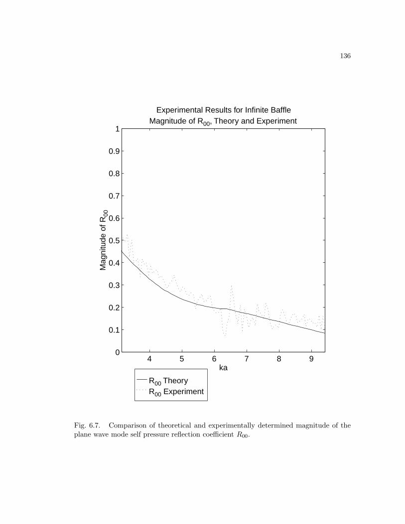
136
R00 Theory R00 Experiment
4 5 6 7 8 90
0.1
0.2
0.3
0.4
0.5
0.6
0.7
0.8
0.9
1
ka
Experimental Results for Infinite BaffleMagnitude of R00, Theory and Experiment
Mag
nitu
de o
f R00
Fig. 6.7. Comparison of theoretical and experimentally determined magnitude of theplane wave mode self pressure reflection coefficient R00.

137
R11 Theory R11 Experiment
4 5 6 7 8 90
0.1
0.2
0.3
0.4
0.5
0.6
0.7
0.8
0.9
1
ka
Experimental Results for Infinite BaffleMagnitude of R11, Theory and Experiment
Mag
nitu
de o
f R11
Fig. 6.8. Comparison of theoretical and experimentally determined magnitude of thefirst mode self pressure reflection coefficient R11.

138
R20 Theory R20 Experiment
6.5 7 7.5 8 8.5 90
0.1
0.2
0.3
0.4
0.5
0.6
0.7
0.8
0.9
1
ka
Experimental Results for Infinite BaffleMagnitude of R20, Theory and Experiment
Mag
nitu
de o
f R20
Fig. 6.9. Comparison of theoretical and experimentally determined mutual pressurereflection coefficient magnitude R20.
139
Chapter 7
Conclusions and Suggestions For Future Research
7.1 Conclusions
While a lot of research has previously been done on duct acoustics, the literature
has been severely lacking in regards to scattering of higher order modes. This thesis will
help to fill the research gap in regards to rigid walled rectangular ducts.
Throughout the thesis, matrix formalisms are used to solve the resulting sets of
simultaneous equations. The simultaneous equations simplify considerably in matrix
form and take on familiar forms.
In chapter 3 the reflection and transmission coefficients at a step discontinuity
were determined in a straight forward manner through the use of generalized scattering
parameters. By solving the problem in this manner both the expansion and constriction
coefficients are determined at the same time. When written in matrix form, the reflection
coefficient equations take the standard form expected for reflection from an impedance
boundary.
The example problems show that the self modal reflection coefficients vary quite
a bit with frequency, often approaching unity at the cut-off frequencies of higher order
modes. The mutual modal reflection coefficients are shown to be quite high at the cut-
off frequency as well, indicating that modal coupling is significant and important in the
analysis of step discontinuities.

140
A more difficult problem, that of a junction, is also handled in a straight forward
manner using generalized scattering parameters in chapter 4. Because the Green’s func-
tion of the junction region is often written as an infinite summation of normal modes,
the problem can be significantly more difficult to solve than the step discontinuity. Us-
ing the matrix form of the equations, the familiar impedance discontinuity form for the
scattering matrix was again obtained.
In the example problems of the right angle bend and the T junction, an infinite
summation from the Green’s function was able to be removed through the use of digamma
functions as shown in appendix A.
The example problems show that the self modal reflection coefficients for a right
angle bend start out at zero, but very quickly rise to large values indicating that a
significant portion of the incident energy is reflected by the bend, even for the plane
wave below the cut-off frequency of the first mode. At and above the cut-off frequency
of a given higher order mode, the transmission coefficient from the plane wave to the
higher order mode is usually more than the plane wave mode self transmission coefficient,
indicating that modal coupling is significant and cannot be ignored in higher frequency
analysis of junctions.
The theoretical solutions for the right angle bend match the experimental results
of Shepherd and Cabelli quite well, with most points within the error of the measurement.
These experimental results verify the junction theory.
141
In chapter 5 radiation impedances and reflection coefficients for a duct terminating
in an infinite baffle were derived. Using the matrix formalism the equation for reflec-
tion coefficients was again shown to take the same form as that of a simple impedance
discontinuity.
The graphs of the amplitude of the radiation impedance should not be too sur-
prising - they are quite similar to that found for circular duct. It is important to note
that above the cut-off frequency of the second mode, the coupling coefficient from the
plane wave mode into the second mode is of higher amplitude than the self reflection
coefficient of the plane wave mode. This indicates that modal coupling cannot be ignored
at frequencies where higher order modes can propagate.
It was shown that the plane wave mode radiates omni-directionally at low fre-
quencies and begins beaming at higher frequencies, while the higher order modes radiate
their energy off axis, with the beams getting closer to the axis at higher frequencies.
Equations for the radiated power were derived in terms of the reflection coefficients
of the duct termination. Using those equations eliminates the complicated integration
of the radiated pressure usually required in determining the radiated power.
The method and results of the experiments were discussed in chapter 6. After
deriving the equations describing how the modal amplitudes could be obtained from
the pressure measurements, there was a discussion of measurement techniques and array
types. It was argued that a horizontal array was probably the best method of determining
modal amplitudes.
Some of the limitations of standard measurement and calibration techniques were
discussed. In particular, it was noted that the use of FFT methods in a highly reverberant
142
environment is fraught with difficulties and experiments may not be repeatable. The use
of complex swept sine analysis was found to reduce the problem.
Plots of experimentally measured reflection coefficients from an infinite baffled
termination were shown along with the theoretical results. The measured plane wave
reflection coefficient was slightly higher in amplitude than the theoretical curve, but
the shape was correct. The measured amplitude of the reflection coefficient of the first
higher order mode matched the theoretical amplitude very well. The measurement of the
mutual coupling coefficient matched theory fairly well. The shape and level were about
the same as theory, but there was far more variance in the mutual coupling coefficient
measurement than with the self reflection coefficient measurement. The match between
theory and experiment is close enough to verify the theory.
Overall, it is clear that modal coupling cannot be ignored at frequencies where
higher order modes can propagate. Mutual modal coupling coefficients are often higher
in amplitude than the modal self reflection coefficients near the cut-off frequency.
7.2 Suggestions for Future Research
The experimental results obtained for the reflection coefficient were adequate
but not exemplary. The strong standing waves at resonances made taking accurate
measurements difficult, even using the swept sine method. Adding damping to the source
end of the duct to reduce the standing waves would probably improve the measurements.
The damping must be confined to the source end so that the region near the baffled end
of the duct still has rigid walls.

143
A knowledge of the approximate error in the measurement would be helpful. The
relative error in the frequency response can be obtained from the coherence function.
The position error can be easily determined. Instead of the simple decomposition al-
gorithm developed in chapter 5, a more complicated algorithm which incorporates the
measurement errors should be used [7]. This would weight measurements with large
error less, and measurements with small errors more. An error bound on the reflection
coefficient computed from the measurements could also be determined.
Because the design of acoustical filters is so important, the method of generalized
parameters could be extended to composite structures. From the generalized parameters
of a cascade of smaller systems, the overall modal response of a system, from input to
output could be determined in a straight forward manner. For example, expansion and
constriction chambers are merely a cascade of two step discontinuities.
Examples of only a few discontinuities were given in the thesis. A more complete
set of scattering coefficients for a number of important discontinuities could be devel-
oped. Handbooks for electro-magnetic waveguides are available which show reflection
and transmission coefficients for a variety of different constructions. With a similar set
of acoustic coefficients the acoustic waveguide designer would be able to quickly choose
the appropriate construct for the desired response.
This thesis derived radiation from a baffled duct. A more difficult and possi-
bly more important problem is to derive expressions for radiation from an unbaffled
duct. Unless a Green’s function for the end of an unbaffled duct can be obtained, the
full Kirchoff-Helmholtz integral will have to be used, resulting in a Fredholm integral
equation which has to be solved. At this time an analytic solution to the problem is

144
unknown. Boundary element or finite element methods could be used to numerically
solve the problem to obtain some theoretical results.

145
Appendix A
Infinite Summations Using Digamma Functions
Infinite summations of the form∑∞n=0
1n2−z2 or
∑∞n=0
(1)n
n2−z2 can be rewritten in
terms of the Digamma function [1, 25, 29].
The Digamma function is defined as
Ψ(z) =d
dzln Γ(z). (A.1)
For z 6= −1,−2,−3, ... the Digamma function can be expanded by the series
Ψ(1 + z) = −γ +∞∑n=1
z
n(n+ z)(A.2)
where γ = 0.577215... is Euler’s constant.
Ψ(1− z) can be subtracted from the above equation to yield the identity
Ψ(1 + z)−Ψ(1− z) = 2z∞∑n=1
1(n2 − z2)
. (A.3)
The Digamma function, like many transcendental functions has various recurrence
formulae (see [25] p.952-956). In particular
Ψ(1 + z) = Ψ(z) +1z
(A.4)

146
Ψ(12
+ z) = Ψ(12− z) + π tan(πz) (A.5)
and
Ψ(1− z) = Ψ(z) + π cot(πz). (A.6)
Subtracting equation A.6 from A.4 yields the identity
Ψ(1 + z)−Ψ(1− z) =1z− π cot(πz). (A.7)
The infinite summation has thus been reduced to a simple equation with well
known functions∞∑n=1
1(n2 − z2)
=12z
[1z− π cot(πz)
]. (A.8)
The infinite summation in H11rm in chapter 4 is then
∞∑n=0
1Λ(n)(n2 − z2)
= −πz
cot(πz). (A.9)
An alternating summation can also be written in terms of the Digamma function
since∞∑n=0
(−1)n
(n+ z)= β(z) =
12
[ψ(
1 + z
2)− ψ(
z
2)]. (A.10)
Using partial fraction expansion and equation A.5
∞∑n=0
(−1)n
(n2 − z2)=
12z
∞∑n=0
(−1)n
(n− z) −(−1)n
(n+ z)=
14z
[Ψ(z
2)−Ψ(−z
2)− π tan(π
z
2)]. (A.11)

147
The remaining two Ψ functions can be removed by using the recurrence relations
to show
Ψ(−z2
) = Ψ(1− z
2)− 2
z= Ψ(
z
2) + π cot(π
z
2). (A.12)
And so finally
∞∑n=0
(−1)n
(n2 − z2)=
14z
[2z− π tan(π
z
2)− π cot(π
2z
)]. (A.13)
With this result the summation for H13rm can be written
∞∑n=0
(−1)n
Λ(n)(n2 − z2)= − π
2z
[tan(π
z
2) + π cot(π
z
2)]. (A.14)

148
Appendix B
Alternate Representation of ZrRM
B.1 Conversion to a Convolution Integral
In chapter 4 it was shown that for a baffled duct the elements of the radiation
impedance matrix are given by the expression
ZrRM =jkρc
2π
∫∫S
∫∫S
ψR(x, y)ψM (x0, y0)e−jk√
(x−x0)2+(y−y0)2√(x− x0)2 + (y − y0)2
dx0dy0dxdy. (B.1)
where ψM (x, y) are the modes of the duct.
Equation B.1 is a four dimensional integral that is often impossible to solve an-
alytically. It can be solved analytically for cylindrical ducts, but not rectangular ducts.
Since the integral is four dimensional and singular whenever x = x0 and y = y0, it may
also be difficult to compute numerically. Using the technique of wavenumber transforms
the integral can be converted into another form which may be computationally easier to
handle.
The Green’s function in B.1, e−jkr/r, is merely a function of the difference in
positions x and x0 and y and y0. The integral over either x and y or x0 and y0 can be
viewed as a convolution integral. To see the convolution integral more clearly, equation
149
B.1 can be rewritten
ZrRM =jkρc
2π
∫∫S
ψR(x, y)
∫∫S
ψM (x0, y0)e−jk√
(x−x0)2+(y−y0)2√(x− x0)2 + (y − y0)2
dx0dy0
dxdy. (B.2)
If ψM (x0, y0) = 0 outside the duct, the term in brackets in equation B.2 is a
convolution integral. Denoting the spatial convolution by ∗ equation B.2 can be rewritten
ZrRM =jkρc
2π
∫∫S
ψR(x, y)
ψM (x0, y0) ∗
e−jk√
(x−x0)2+(y−y0)2√(x− x0)2 + (y − y0)2
dxdy. (B.3)
B.2 Review of Wavenumber Transforms
Just as standard Fourier transforms are a useful tool for analyzing time domain
waveforms, the spatial Fourier transform or wavenumber transform is a useful tool in
analyzing spatial waveforms. In the time domain Fourier transform, time is transformed
into frequency. In the spatial Fourier transform, spatial coordinates are transformed into
wavenumbers, hence the term wavenumber transform.
The forward wavenumber transform is defined as
F (kx, ky, kz, ω) =∫ ∞∫−∞
∫f(x, y, z, ω)e−jkxxe−jkyye−jkzzdxdydz. (B.4)
The inverse wavenumber transform is defined as
f(x, y, z, ω) =1
(2π)3
∫ ∞∫−∞
∫F (kx, ky, kz , ω)ejkxxejkyyejkzzdkxdkydkz. (B.5)

150
Just like time domain Fourier transforms, there is a large number of special prop-
erties associated with wavenumber transforms. One of these properties is the convolution
property.
The convolution theorem of wavenumber transforms as stated in Bracewell [8]
states that the wavenumber transform of the convolution of two functions is the product
of their wavenumber transforms. In two dimensions the convolution integral is written
f(x, y) ∗ g(x, y) =∫∞∫−∞
f(x′, y′)g(x− x′, y − y′)dx′dy′ (B.6)
=1
(2π)2
∫∞∫−∞
F (kx, ky)G(kx, ky)× ejkxxejkyydkxdky. (B.7)
For a baffled duct the Green’s function is G(x− x0, y − y0) = e−jkr/r, where the
distance r =√
(x− x0)2 + (y − y0)2. The wavenumber transform of the baffled Green’s
function is then
Gk(kx, ky) =∫∞∫−∞
e−jk√
(x−x0)2+(y−y0)2√(x− x0)2 + (y − y0)2
e−jkxxe−jkyydx0dy0 =−jejkxxejkyy√k2 − k2
x − k2y
. (B.8)
In computing the wavenumber transform of ψM (x, y) it must be noted that
ψM (x, y) is confined to the duct region. It is standard practice to define ψM (x, y) = 0
outside the duct.With this definition the wavenumber transform of of ψM (x, y) is
ΨM (kx, ky) =∫∞∫−∞
ψM (x, y)e−jkxxe−jkyydxdy =∫∫S
ψM (x, y)e−jkxxe−jkyydxdy. (B.9)
151
B.3 Transformation of ZrRM
Using the wavenumber transform for the Green’s function and the convolution
property of wavenumber transforms discussed above, equation B.3 can be rewritten as
ZrRM =kρc
4π2
∫∫S
ψR(x, y)
∫∞∫−∞
ΨM (kx, ky)√k2 − k2
x − k2y
ejkxxejkyydkxdky
dxdy (B.10)
where ΨM (kx, ky) is the wavenumber transform of ψM (x, y).
This can be rearranged once again to form
ZrRM =kρc
4π2
∫∞∫−∞
ΨM (kx, ky)√k2 − k2
x − k2y
∫∫S
ψR(x, y)ejkxxejkyydkxdky
dxdy. (B.11)
The remaining spatial integral is the same as equation B.9 with kx replace by −kx
and ky replaced by −ky. So, one can replace the spatial integration with ΨM (−kx,−ky)
to yield
ZrRM =kρc
4π2
∫∞∫−∞
ΨM (kx, ky)ΨR(−kx,−ky)√k2 − k2
x − k2y
ejkxxejkyydkxdky. (B.12)
At this point a finite four dimensional integral which was singular at many points
has been reduced to a two dimensional infinite integral which is also singular at many
points. This may or may not be easier to deal with computationally. But, the integral
can be reduced once again by rewriting it in polar coordinates. The final result is
ZrRM =kρc
4π2
∫ ∞0
∫ 2π
0
ΨM (µ cos θ, µ sin θ)ΨR(−µ cos θ,−µ sin θ)√k2 − µ2
µdµdθ. (B.13)
where kx = µ cos θ and ky = µ sin θ.
152
This two dimensional integral is infinite in only one dimension and is singular at
only one point. Depending upon the form of ΨM(kx, ky) equation B.13 may be much
easier to compute than B.1 or B.12.
B.4 Application to a Rectangular Duct
For a rectangular duct the ψM (x, y) = cos(mxπa ) cos(myπb ). In order compute
ZrRM using equations B.12 or B.13 the wavenumber transform ΨM (kx, ky) must be
computed.
ΨM (kx, ky) =a∫
0
b∫0
cos(mxπa x) cos(myπb y)√abΛmxΛmy
e−jkxxe−jkyydxdy. (B.14)
When mxπa 6= kx and myπ
b 6= ky
ΨM (kx, ky) =−kxky[1− (−1)mxe−jkxa][1− (−1)mye−jkyb]√
abΛmxΛmy [(mxπa )2 − k2x][(myπb )2 − k2
y ]. (B.15)
When mxπa = kx but myπ
b 6= ky
ΨM (kx, ky) =j√aky[1− (−1)mye−jkyb]√bΛmy [(myπb )2 − k2
y ]. (B.16)
When mxπa 6= kx but myπ
b = ky
ΨM (kx, ky) =j√bkx[1− (−1)mxe−jkxa]√aΛmx [(mxπa )2 − k2
x]. (B.17)
153
When mxπa = kx and myπ
b = ky
ΨM (kx, ky) =√ab. (B.18)
As a check one can look at the M = 0, R = 0 term of ZrRM . That term is the
radiation impedance of a of a rectangular piston.
For M = 0 (mx = 0,my = 0) and R = 0 (rx = 0, ry = 0) kM = k and the
wavenumber transform of the mode becomes
Ψ(kx, ky) =√abe−jkx
a2 e−jy
b2 sinc(kxa/2)(sinc(kyb/2). (B.19)
and equation B.12 becomes
Zr00 =kρc(ab)
4π2
∫∞∫−∞
sinc2(kxa/2)sinc2(kyb/2)√k2 − k2
x − k2y
dkxdky
=kρc(ab)
4π2
∫ ∞0
µdµ√k2 − µ2
∫ 2π
0sinc2(
µa cos θ2
)sinc2(µb sin θ
2)dθ. (B.20)
This is very similar to the equation derived by Morse and Ingard [44] in their
development of the the radiation impedance of a square piston. (Morse and Ingard
never explicitly derive the radiation impedance in an exact form. In equation 7.4.43
they derive and expression for the force on the piston in terms of the piston velocity.
The radiation impedance can be obtained by dividing the force by the velocity and the
area of the piston. The resulting equation is the same as B.20. Also note that equation
7.4.43 of [44] is missing a square root over the denominator of the integral.)
154
Appendix C
Numerical Integration of ζRM
Recall that for a rectangular duct, the equation for ζRM is
ζRM =jkρc
2π
a∫0
b∫0
a∫0
b∫0
cos(mxπa x)√aΛmx
cos(myπb y)√bΛmy
cos(mxπa x0)√aΛmx
cos(myπb y0)√bΛmy
e−jkr
rdx0dy0dxdy.
(C.1)
Numerical evaluation of C.1 is not an easy process. While the four dimensional
integral looks straight forward, the integrand is singular, so caution must be taken.
At frequencies low enough for only a few modes to propagate, an approximation
to the integral in equation C.1 can be obtained by discretization of the region into
sub-regions and approximating the integral over each sub-region. Then the integral is
obtained by summation of the portion from each sub-region.
If the end of the duct is broken into a series of rectangular regions of size 2 α by
2 β equation C.1 becomes
ζRM =jkρc
2π
∑µ
∑ν
Iµν (C.2)
where
Iµν =α∫−α
β∫−β
α∫−α
β∫−β
ψR(xµ + εx, yµ + εy)ψM (xν + δx, yν + δy)e−jkr
rdεxdεydδxdδy. (C.3)
155
The integrals in equation C.3 can be approximated for both µ 6= ν and µ = ν.
For µ 6= ν standard Gaussian quadratures can be used to compute the integral
over this sub-region [51].
For µ = ν the integral in equation C.3 is singular. However, the singularity must
be integrable because physically it is known that ζRM is not infinite. The singularity can
be removed by a transformation into polar coordinates, but the resulting integral is still
difficult to do numerically. An alternate change of variables is used by CHIEF, a program
which was written to solve the integral equations resulting from acoustic radiation from
a general vibrating surface [6].
Consider an integral over a rectangular region of the form
I =uu∫ul
vu∫vl
F (u′, v′)du′dv′. (C.4)
The u′− v′ region can be broken into four triangular regions T1, T2, T3, and T4 as
shown in figure C.1.
Then, the integral becomes
I =∫∫T1
+∫∫T2
+∫∫T3
+∫∫T4
Fdu′dv′. (C.5)
Assume that the integral is singular at the center of the rectangle, at u′0 = (uu −
ul)/2 and v′0 = (vu − vl)/2.
Consider the following change of variables in region T1:
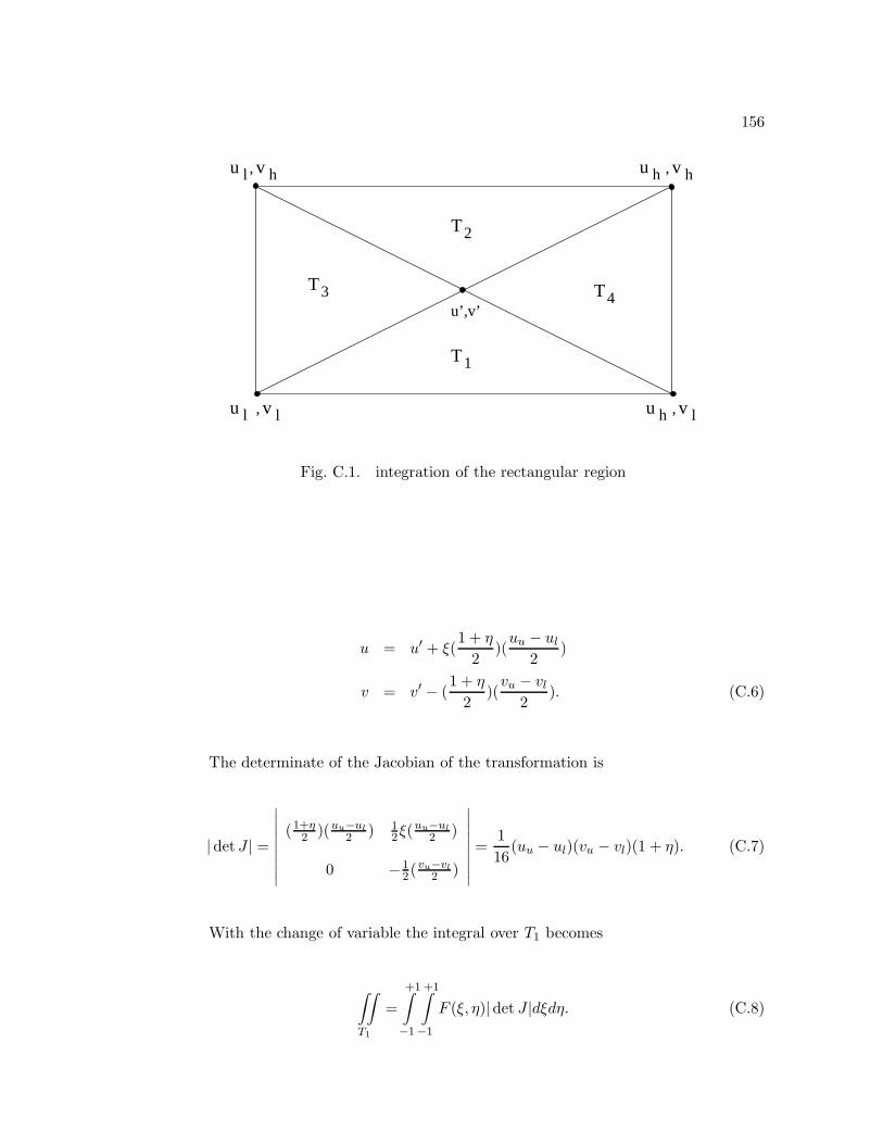
156
u h , v lu l v l,
u h v h,v hu l ,
T3 T4
T1
T2
u’,v’
Fig. C.1. integration of the rectangular region
u = u′ + ξ(1 + η
2)(uu − ul
2)
v = v′ − (1 + η
2)(vu − vl
2). (C.6)
The determinate of the Jacobian of the transformation is
|det J | =
∣∣∣∣∣∣∣∣∣(1+η
2 )(uu−ul2 ) 12ξ(
uu−ul2 )
0 −12(vu−vl2 )
∣∣∣∣∣∣∣∣∣ =116
(uu − ul)(vu − vl)(1 + η). (C.7)
With the change of variable the integral over T1 becomes
∫∫T1
=+1∫−1
+1∫−1
F (ξ, η)|det J |dξdη. (C.8)
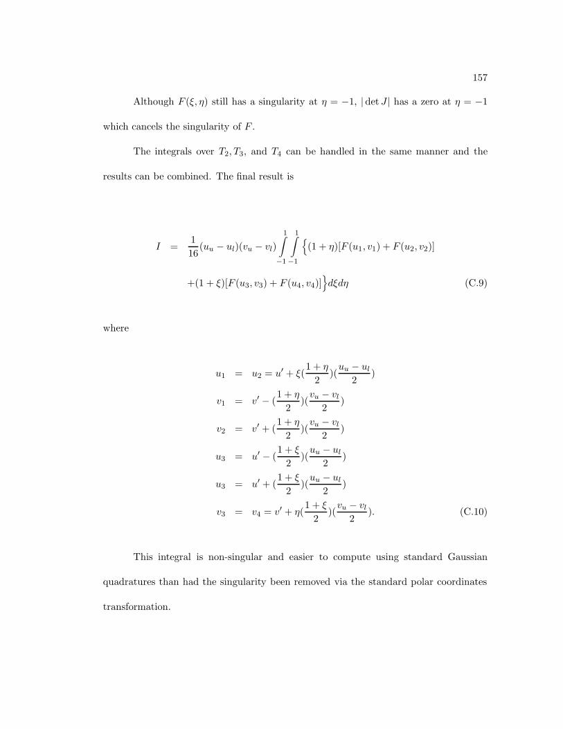
157
Although F (ξ, η) still has a singularity at η = −1, |det J | has a zero at η = −1
which cancels the singularity of F .
The integrals over T2, T3, and T4 can be handled in the same manner and the
results can be combined. The final result is
I =116
(uu − ul)(vu − vl)1∫−1
1∫−1
{(1 + η)[F (u1, v1) + F (u2, v2)]
+(1 + ξ)[F (u3, v3) + F (u4, v4)]}dξdη (C.9)
where
u1 = u2 = u′ + ξ(1 + η
2)(uu − ul
2)
v1 = v′ − (1 + η
2)(vu − vl
2)
v2 = v′ + (1 + η
2)(vu − vl
2)
u3 = u′ − (1 + ξ
2)(uu − ul
2)
u3 = u′ + (1 + ξ
2)(uu − ul
2)
v3 = v4 = v′ + η(1 + ξ
2)(vu − vl
2). (C.10)
This integral is non-singular and easier to compute using standard Gaussian
quadratures than had the singularity been removed via the standard polar coordinates
transformation.
158
References
[1] Milton Abramowitz and Irene A. Stegun. Handbook of Mathematical Functions.
Dover, New York, 1965.
[2] George Arfken. Mathematical Methods for Physicists, Third Edition. Academic
Press, 1985.
[3] David C. Baumann and R. A. Greiner. Modal identification approach to multi-
modal cancellation. In Proceedings of Internoise 92, pages 341–344, 1992.
[4] David C. Baumann and R. A. Greiner. Number of error microphones for multi-
modal cancellation. In Proceedings of Internoise 92, pages 345–348, 1992.
[5] Julius S. Bendat and Allan G. Piersol. Engineering Applications of Correlation And
Spectral Analysis. Wiley Interscience, New York, 2 edition, 1993.
[6] G. Benthien, D. Barach, and D. Gillette. CHIEF Users Manual, NOSC Technical
Document 970. Naval Ocean Systems Center, 1988.
[7] P. R. Bevington. Data Reduction and Error Analysis for the Physical Sciences.
McGraw Hill, New York, 1969.
[8] Ronald N. Bracewell. The Fourier Transform and its Applications. McGraw Hill,
New York, 1978.

159
[9] Jan C. Bruggeman. The propagation of low-frequency sound in a two-dimensional
duct system with t joints and right angle bends: Theory and experiment. Journal
of the Acoustical Society of America, 82(3):1045–1051, 1987.
[10] Herbert J. Carlin and Anthony B. Giordano. Network Theory, An Introduction to
Reciprocal and Nonreciprocal Circuits. Prentice Hall, Englewood Cliffs, NJ, 1964.
[11] R. E. Collins. Foundations for Microwave Engineering. McGraw-Hill, New York,
1966.
[12] R. Courant and D. Hilbert. Methods of Mathematical Physics, volume 1. Wiley,
1989.
[13] R. Courant and D. Hilbert. Methods of Mathematical Physics, volume 2. Wiley,
1989.
[14] A. Craggs. A finite element method for damped acoustic systems: An application
to evaluate the performance of reactive mufflers. Journal of Sound and Vibration,
48(3):377–392, 1976.
[15] A. Craggs. The application of the transfer matrix and matrix condensation methods
with finite elements to duct acoustics. Journal of Sound and Vibration, 132(2):393–
402, 1989.
[16] D.G. Crighton, A. P. Dowling, J. E. Ffowcs Williams, M. Heckl, and F. G. Lepping-
ton. Modern Methods in Analytical Acoustics. Springer-Verlag, 1992.
160
[17] A. Cummings. Sound transmission in 180 ◦ duct bends of rectangular section.
Journal of Sound and Vibration, 41(3):321–332, 1975.
[18] P. E. Doak. Excitation, transmission and radiation of sound from source distri-
butions in hard-walled ducts of finite length (i): The effects of duct cross-section
geometry and source distription space-time pattern. Journal of Sound and Vibra-
tion, 31(1):1–72, 1973.
[19] P. E. Doak. Excitation, transmission and radiation of sound from source distribu-
tions in hard-walled ducts of finite length (ii): The effects of duct length. Journal
of Sound and Vibration, 31(2):137–174, 1973.
[20] Frank Fahy. Sound and Structural Vibration. Academic Press, London, 1993.
[21] D. Firth and F. J. Fahy. Acoustic characteristic of ciruclar bends in pipes. Journal
of Sound and Vibration, 97(2):287–303, 1984.
[22] C. R. Fuller. Propagation and radiation of sound from flanged circular ducts with
circumferentially varying wall admittances, i: Semi-infinite ducts. Journal of Sound
and Vibration, 93(3):321–340, 1984.
[23] G. D. Furnell and D. A. Bies. Characteristics of modal wave propagatin within longi-
tudinally curved acoustic waveguides. Journal of Sound and Vibration, 130(3):405–
423, 1989.
[24] G. D. Furnell and D. A. Bies. Matrix analysis of acoustic wave propagation within
curved ducting systems. Journal of Sound and Vibration, 132(2):245–263, 1989.

161
[25] I. S. Gradshteyn and I. M. Ryzhik. Table of Integrals, Series, and Products. Aca-
demic Press, London, 5 edition, 1994.
[26] Herbert Hudde. Acoustical higher order mode scattering matrix of circular nonuni-
form lossy tubes without flow. Journal of the Acoustical Society of America,
85(6):2316–2330, 1989.
[27] Herbert Hudde and Uwe Letens. Scattering matrix of a discontinuity with a non-
rigid wall in a lossless circular duct. Journal of the Acoustical Society of America,
78(5):1826–1837, 1985.
[28] Tatsuo Itoh, editor. Numerical Techniques for Microwave and Millimeter-Wave
Passive Structures. Wiley-Interscience, New York, 1989.
[29] L. B. W. Jolley. Summation of Series. Dover, New York, 1961.
[30] Miguel C. Junger and David Feit. Sound, Structures and Their Interaction. MIT
Press, Cambridge, Massachussettes, second edition, 1986.
[31] Cornelius Lanczos. Linear Differential Operators. Van Nostrad, 1961.
[32] Harold Levine and Julian Schwinger. On the radiation of sound from an unflanged
circular duct. Physical Review, 73(4):383–406, 1948.
[33] W. K. Lippert. A method of measuring discontinuity effects in ducts. Acoustica,
4(2):308–312, 1954.
[34] W. K. Lippert. The meadurement of sound reflection and transmission at right-
angled bends in rectangular tubes. Acoustica, 4(2):314–318, 1954.

162
[35] Robert H. Macphie and Amir I. Zaghloul. Radiation form a rectangualr waveg-
uide with infintie flange - exact solution by the correlation matrix method. IEEE
Transactions on Microwave Theory and Techniques, 28(4):497–503, 1980.
[36] W. P. Mason. A study of the regular combination of acoustic element, with appli-
cations to recurrent acoustic filters, taper acoustic filters, and horns. Bell System
Technical Journal, 6:258–275, 1927.
[37] W. L. Meyer and B. T. Zinn. Sound radiation from fitie length axissymmetric ducts.
Journal of Sound and Vibration, 90(2):286–290, 1983.
[38] John W. Miles. The analysis of plane discontinuities in cylindrical tubes. part i.
Journal of the Acoustical Society of America, 17(3):259–271, 1945.
[39] John W. Miles. The analysis of plane discontinuities in cylindrical tubes. part ii.
Journal of the Acoustical Society of America, 17(3):272–284, 1945.
[40] John W. Miles. The diffraction of sound due to right-angled joints in rectangular
tubes. Journal of the Acoustical Society of America, 19(4):572–579, 1947.
[41] R. Mittra and S. W. Lee. Analytical Techniques in the Theory of Guided Waves.
The MacMillan Company, 1971.
[42] Philip M. Morse and Herman Feshbach. Methods of Theoretical Physics, volume 2.
McGraw Hill, 1953.
[43] Philip M. Morse and Herman Feshbach. Methods of Theoretical Physics, volume 1.
McGraw Hill, 1953.

163
[44] Philip M. Morse and K. Uno Ingard. Theoretical Acoustics. Princeton Univerisity
Press, Princeton, New Jersey, 1968.
[45] Ralph T. Muehleisen and David C. Swanson. An impedance model for actively con-
trolled finite waveguides. Journal of the Acoustical Society of America, 91(4):2349,
1992.
[46] M. L. Munjal. Acoustics of Ducts and Mufflers. John Wiley and Sons, 1987.
[47] B. Noble. Methods based on The Wiener-Hopf Technique for the solution of partial
differential equations. Pergamon Press Inc., 1958.
[48] A. N. Norris and I. C. Sheng. Acoustic radiation from a circular pipe with an infinite
flange. Journal of Sound and Vibration, 135(1):85–93, 1989.
[49] T. Okoshi. Planar Circuits for Microwaves and Lightwaves. Springer-Verlag, Berlin,
1985.
[50] Allan D. Pierce. Acoustics - An Introduction into Its Physical Principles and Appli-
cations. Acoustical Society of America, Woodbury, New York, 1989 edition, 1989.
[51] William H. Press, Saul A. Teukolsky, William T. Vetterling, and Brian P. Flannery.
Numerical Recipies in Fortran. Cambridge University Press, 2 edition, 1992.
[52] J. W. S. Rayleigh. The Theory of Sound, volume 2. Dover, New York, 1945.
[53] J. W. S. Rayleigh. The Theory of Sound, volume 1. Dover, New York, 1945.

164
[54] T. L. Redmore and K. A. Mulholland. The application of mode coupling theory to
the transmission of sound in the sidebrance of a rectangualar duct system. Journal
of Sound and Vibration, 85(3):323–331, 1982.
[55] S. P. Rubenstein, S. R. Popovich, D. E. Melton, and M. C. Allie. Active cancellation
of higher order modes in a duct using recursively-coupled multi-channel adaptive
control system. In Proceedings of Internoise 92, pages 337–340, 1992.
[56] Reza Safavi-Naini and Robert H. Macphie. On solving waveguide junction scattering
problems by the conservation of complex power techniques. IEEE Transactions on
Microwave Theory and Techniques, 29(4):337–343, 1981.
[57] Reza Safavi-Naini and Robert H. Macphie. Scattering at rectangular-to-rectangular
waveguide junctions. IEEE Transactions on Microwave Theory and Techniques,
30(11):2060–2063, 1982.
[58] A. Said. Theorie der schallausbreitun in kanalen mit rechtwinkligen ecken und
verzweigungen. Acoustica, 33(2):203–210, 1975.
[59] I. C. Shepherd and A. Cabelli. Transmission and reflection of higher order acoustic
modes in a mitred duct bend. Journal of Sound and Vibration, 77(4):495–511, 1981.
[60] I. C. Shepherd and A. Cabelli. Duct acoustics - a numerical technique for the
higher order mode solution of three-dimensional problems with rigid walls and no
flow. Journal of Sound and Vibration, 92(3):419–426, 1984.
165
[61] R. J. Silcox. Active control of multi-modal random sound in ducts. Technical report,
NASA Langley Research Center.
[62] J. D. Stell and R. J. Bernhard. Active control of high order acoustical modes
in a seminfinite waveguide. Transactions of the ASME, Journal of Vibration and
Acoustics, 113:523–531, 1991.
[63] J. D. Stell and R. J. Bernhard. Active control of sound in acoustic waveguides, part
i: Theory. Journal of Sound and Vibration, 173(2):179–196, 1994.
[64] J. D. Stell and R. J. Bernhard. Active control of sound in acoustic waveguides, part
ii: Considerations for implementation in ducts. Journal of Sound and Vibration,
173(2):197–215, 1994.
[65] J. Tichy, G. E. Warneka, and L. A. Poole. A study of active control of noise in ducts.
Transactions of the ASME, Journal of Vibration, Acoustics, Stress, and Reliability
in Design, 106:399–404, 1984.
[66] C. E. Wallace. Radiation resistance of a rectangular panel. Journal of the Acoustical
Society of America, 51(3):946–952, 1972.
[67] K. S. Wang and T. C. Tszeng. Propagation and radiation of sound in a finite length
duct. Journal of Sound and Vibration, 93(1):57–79, 1984.
[68] Lev Albertovich Weinstein. The Theory of Diffraction and The Factorization
Method. The Golem Press, Boulder, Colorado, 1969.

166
[69] Erich Zauderer. Partial Differential Equations of Applied Mathematics. Wiley-
Interscience, New York, 1983.
[70] William E. Zorumski. Generalized radiation impedances and reflection coefficients of
circular and annular ducts. Journal of the Acoustical Society of America, 54(6):1667–
1673, 1973.
Vita
Ralph Terry Muehleisen was born in Oconomowoc, Wisconsin on February 10,
1967. He graduated from Arrowhead High School in Hartland, Wisconsin in June of
1985. He began studies at the University of Wisconsin - Madison in August 1985. He
married Sally Laurent in May of 1989. He received the Bachelor of Science degree
from the University of Wisconsin - Madison with majors in Electrical and Computer
Engineering and Physics in December of 1989. As a student he worked as a lab assistant
in the Physics department on the Madison Symmetric Torus plasma fusion device. He
also worked in the Electroacoustic Lab in the Department of Electrical and Computer
Engineering. He began studies in the Graduate Program in Acoustics at Penn State
in August of 1990. Upon completion of his degree Ralph plans to pursue Postdoctoral
studies with his thesis advisor David Swanson at the Penn State Applied Research Lab.
During his undergraduate and graduate studies Ralph has received numerous
awards. As an undergraduate he received an “Outstanding Tutor Award” in 1988 from
the University of Wisconsin - Madison physics club. He was a “Dean’s Fellow” of the
College of Engineering at Penn State from 1990-1992. He received a “Graduate School
Fellowship Honorable Mention” from the Penn State Graduate School in 1993. He re-
ceived the “Outstanding Presentation by a Young Professional” award and a “Physical
Acoustics Summer School Fellowship” from the Acoustical Society of America in 1992.
Ralph is a member of ASA, IEEE, the Audio Engineering Society and the Institute
of Noise Control Engineers.
Copyright © 2022 FDOKUMEN