Adaptive detection and approximation of unknown

surface discontinuities from scattered data

G. Allasia, R. Besenghi, and R. Cavoretto

Department of Mathematics,University of Turin,

via Carlo Alberto 10, 10123 Torino, ItalyE-mail: giampietro.allasia, renata.besenghi, roberto.cavoretto@unito.it

Abstract

We consider a method for the detection and approximation of faultlines of a surface, which is known only on a finite number of scattereddata. In particular, we present an adaptive approach to detect surfacediscontinuities, which allows us to give an (accurate) approximation ofthe detected faults. First, to locate all the nodes close to fault lines, weconsider a procedure based on a local interpolation scheme involvinga cardinal radial basis formula. Second, we find further sets of pointsgenerally closer to the faults than the fault points. Finally, after apply-ing a nearest-neighbor searching procedure and a powerful refinementtechnique, we outline some different approximation methods. Numer-ical results highlight the efficiency of our approach.

Keywords: scattered data, surface discontinuities, adaptive detection,approximation methods, radial basis functions.

Mathematics Subject Classification 2000: 65D05, 65D10, 65D17.

1 Introduction

In this paper we propose an adaptive approach for the detection and approx-imation of surface discontinuities, which are known only on a finite numberof scattered data. In geology a surface discontinuity is often named with theword “fault”, which means discontinuity in a layer caused by severe move-ments of the earth’s crust. In geological applications, such as oil finding,fault localization is particularly important, because it provides useful infor-mation on the occurrence of oil reservoirs [10]. It is well known that theinterpretation of faults in seismic data is today a time-consuming manualtask, and reducing time from exploration to production of an oil field hasgreat economical benefits [11].

1

Besides geology, the problem of detecting surface discontinuities, oftenreferred as fault lines or edges (i.e. jumps in a surface), is encounteredfrequently in a wide variety of scientific fields, such as image processing,medicine, geophysics, oceanography, tomography, cartography, etc.. Eitherthe fault detecting and approximating problem, or the discontinuous surfaceapproximating problem have been dealt with extensively in the literatureand several authors have proposed different techniques and methodologies(see, for instance, [5, 16, 13, 8, 9, 15, 12] and references therein).

In the following, for simplicity, we will consider surface discontinuities ofthe type of geological vertical faults and will refer to these simply as faults.

In [2] we presented a method for the localization of unknown fault linesof a surface, moving from a large set of data points or nodes irregularlydistributed in a plane region and the corresponding function values. In thepresent paper we improve the detection scheme proposed in [2], introducingan adaptive detection process (see Section 5 for more details). Moreover, wediscuss different methods to approximate fault lines, considering polygonallines, least squares, and best l∞ approximations [3].

Note that in some real applications, e.g. in geology, the searching ofinformation, i.e. discontinuity points, can be very expensive, since it isrequired to drill or explode mines in subsoil. Moreover, in general, one doesnot know the location of the fault lines on the surface or even whether or notthe surface is faulted [4]. So, the adaptive procedure can reveal itself veryuseful, because this approach produces a considerable reduction of cost.

The paper is organized as follows. In Section 2 we explain the detectionalgorithm for the fault lines, relating to cardinal radial basis interpolants(CRBIs), whose properties are widely discussed in [1]. In Section 3 webriefly describe the different techniques of approximation. Section 4 con-tains some useful remarks. In Section 5 several numerical results show theeffectiveness of our approach. Finally, in Section 6, we give an idea of pos-sible developments.

2 Detection Scheme

In this section we present the basic ideas which allow us to pick out the datapoints on or close to the fault lines, named fault points. To characterizethese points, first, we consider a procedure based on local data interpolationby CRBIs, where the difference between any known function value and therelated value of the interpolant is computed and compared with a thresholdparameter. Second, we introduce and define a new set of points, namedbarycentres, generally closer to the faults than the fault points. Finally,manipulating the barycentres, we find further sets of points subjected ornot to any refinement. They supply more information on the faults.

Let Sn = {Pk, k = 1, . . . , n} be a set of distinct and scattered data

2

points in a domain D ⊂ R2, and {f(Pk), k = 1, . . . , n} a set of corresponding

values of an unknown function f : D → R, which is discontinuous across aset Γ = {Γj , j = 1, . . . , m} of fault lines

Γj = {γj(t) : t ∈ [0, 1]} ⊂ D,

where γj are unknown parametric continuous curves. On D \Γ the functionf is supposed to be smooth. The domain D is bounded, closed, simplyconnected, and contains the convex hull of Sn.

The detection algorithm is divided into five steps:

(i) A cell-based search method is applied to find the data point set NPk

neighboring to each node Pk of the data set Sn [6]. It is a classical nearest-neighbor searching procedure, in which we make a subdivision of the domainD in cells and identify the points closest to a data point within each cell.Then, to determine the fault points, a CRBI is built on each set NPk

, (k =1, . . . , n), excluding Pk. As a significant example of CRBI we recall Shepard’sformula (see [1])

F (x) =n

∑

i=1

fi

d(x, xi)−p

∑nj=1 d(x, xj)−p

, F (xi) = fi, i = 1, . . . , n,

where d(x, xi) is the Euclidean distance in R2 and p > 0.

(ii) We evaluate the absolute value of the difference σ(Pk) between thefunction value f(Pk) and the value of the interpolant at Pk, viz. σ(Pk) =|f(Pk) − F (Pk)|. Supposing the interpolant gives a good approximation to fin D, then σ(Pk) gives a measure of the smoothness of the function aroundPk. If we choose a suitable threshold value σ0 > 0, we can compare thevalues σ(Pk) and σ0: σ(Pk) is less than or equal to σ0 when f is smooth in aneighborhood of Pk, otherwise it is greater than σ0 when a steep variation off at Pk is found, and accordingly Pk will be marked as a fault point. Whenthe detection procedure of the nodes is concluded, we have characterized theset of fault points F(f ; Sn) = {Pk ∈ Sn : σ(Pk) > σ0} consisting of all thenodes either belonging to the faults or, at least, close to them.

(iii) Given a fault point Pk ∈ F(f ; Sn) and the corresponding nearest-neigh-bor set NPk

, we define DPk= {P ∈ D : d(P, Pk) ≤ RPk

}, where RPk=

max{d(Pi, Pk) : Pi ∈ NPk}. Then we order the NPk

+ 1 points in NPk

= NPk∪ {Pk}, being NPk

= card(NPk), so that f(Pk1) ≤ f(Pk2) ≤ · · ·

≤ f(PkNPk+1). The expected jump δk of f in the subdomain DPk

is evaluatedby

δk = max1≤l≤NPk

∆f(Pkl),

where ∆ is the forward difference operator. We set lk the lowest value ofthe index l ∈ {1, . . . , NPk

} for which δk is obtained.

3

The part Πk = DPk∩Γ of a fault line separates the set ∆L

k = {Q ∈ NPk:

f(Q) ≤ f(Pklk)} of all nodes of NPkwith lower function values from the set

∆Hk = {Q ∈ NPk

: f(Q) > f(Pklk)} of all nodes of NPkwith higher function

values. If ∆Lk or ∆H

k is the empty set, then we enlarge NPkand repeat the

process, so that NPkcontains points lying in the two parts of the subdomain

separated by the fault line. Having determined ∆Lk and ∆H

k in this way, wecalculate the barycentres AL

k and AHk of ∆L

k and ∆Hk , respectively. Then we

find Ak = (ALk + AH

k )/2 and put it in A(f ; Sn), the set of the barycentres.

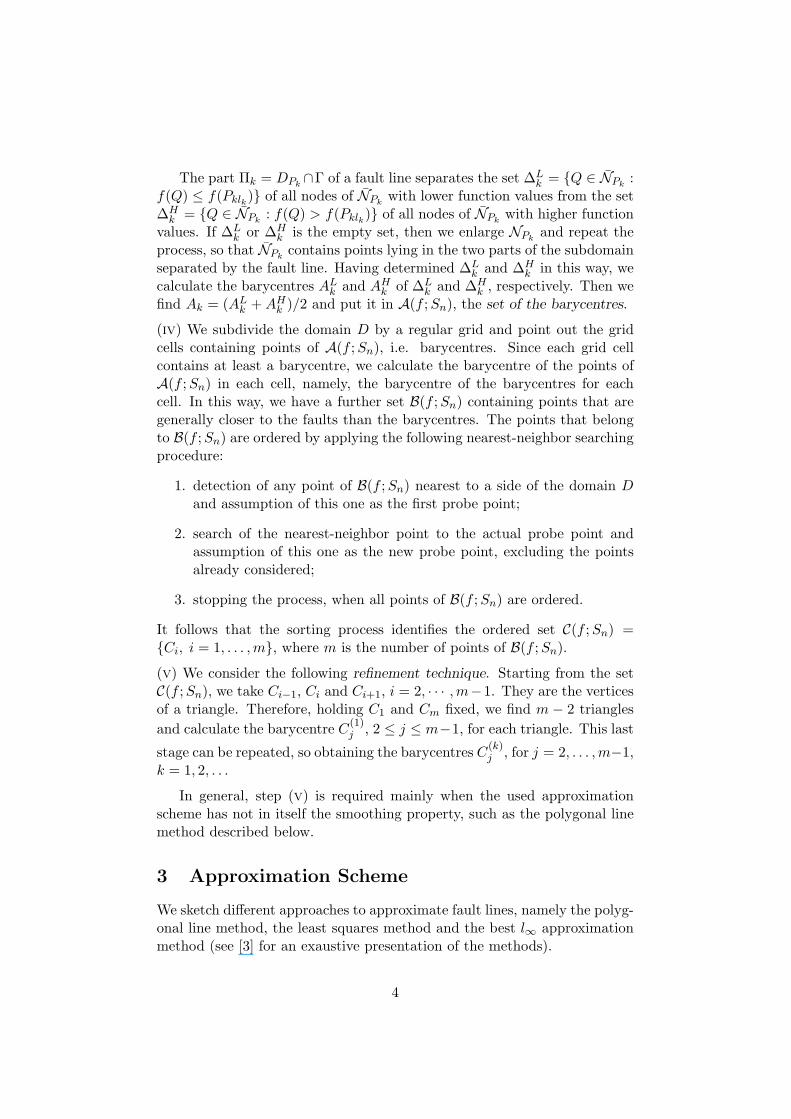
(iv) We subdivide the domain D by a regular grid and point out the gridcells containing points of A(f ; Sn), i.e. barycentres. Since each grid cellcontains at least a barycentre, we calculate the barycentre of the points ofA(f ; Sn) in each cell, namely, the barycentre of the barycentres for eachcell. In this way, we have a further set B(f ; Sn) containing points that aregenerally closer to the faults than the barycentres. The points that belongto B(f ; Sn) are ordered by applying the following nearest-neighbor searchingprocedure:

1. detection of any point of B(f ; Sn) nearest to a side of the domain Dand assumption of this one as the first probe point;

2. search of the nearest-neighbor point to the actual probe point andassumption of this one as the new probe point, excluding the pointsalready considered;

3. stopping the process, when all points of B(f ; Sn) are ordered.

It follows that the sorting process identifies the ordered set C(f ; Sn) ={Ci, i = 1, . . . , m}, where m is the number of points of B(f ; Sn).

(v) We consider the following refinement technique. Starting from the setC(f ; Sn), we take Ci−1, Ci and Ci+1, i = 2, · · · , m−1. They are the verticesof a triangle. Therefore, holding C1 and Cm fixed, we find m − 2 triangles

and calculate the barycentre C(1)j , 2 ≤ j ≤ m−1, for each triangle. This last

stage can be repeated, so obtaining the barycentres C(k)j , for j = 2, . . . , m−1,

k = 1, 2, . . .

In general, step (v) is required mainly when the used approximationscheme has not in itself the smoothing property, such as the polygonal linemethod described below.

3 Approximation Scheme

We sketch different approaches to approximate fault lines, namely the polyg-onal line method, the least squares method and the best l∞ approximationmethod (see [3] for an exaustive presentation of the methods).

4

Polygonal line method. The polygonal line method we consider repre-sents an improvement of the procedures developed by Gutzmer and Iske [13]and by Allasia, Besenghi and De Rossi [2].

The ordered points of C(f ; Sn) are connected by straight line segments,obtaining a polygonal line which approximates the fault line.

Least squares method. The least squares method can be used to approx-imate a data set, {(xi, yi), i = 1, . . . , m} by an algebraic polynomial

Ps(x) = c0 + c1x + · · · + cs−1xs−1 + csx

s (1)

of degree s < m − 1. In our problem we choose the constants c0, c1, . . . , cs

to solve the least squares problem

minc0,...,cs

m∑

i=1

[yi − Ps(xi)]2 ,

where (xi, yi) ∈ C(f ; Sn). Replacing the coefficients c0, c1, . . . , cs in (1) withthe values obtained by the least squares method, we get the polynomialapproximating the fault line.

Best l∞ approximation method. The best l∞ approximation methodcan be considered as a tool for finding polynomial approximations to faultlines starting from the set C(f ; Sn) or from some its refinement.

Given the abscissae xk and the corresponding ordinates yk, for k =1, 2, . . . , m, the polynomial in (1) is sought to solve the minimax problem

minc0,...,cs

maxk

|Ps(xk) − yk| . (2)

Denoting by M = maxk |Ps(xk)−yk| > 0 the largest absolute value, we have

|Ps(xk) − yk| ≤ M, k = 1, 2, . . . , m, (3)

and the inequalities (3) can be rewritten in the form

∣

∣

∣

∣

∣

∣

s∑

j=0

( cj

M

)

xjk −

(

1

M

)

yk

∣

∣

∣

∣

∣

∣

≤ 1, k = 1, 2, . . . , m.

The linear programming problem (2) becomes

maximize Z = ts+2,

subject to the constraints

t1 + xkt2 + x2kt3 + . . . + xs

kts+1 − ykts+2 ≤ 1,

t1 + xkt2 + x2kt3 + . . . + xs

kts+1 − ykts+2 ≥ −1,

5

for k = 1, 2, . . . , m, andts+2 ≥ 0,

with the unknowns

t1 =c0

M, t2 =

c1

M, t3 =

c2

M, . . . , ts+1 =

cs

M, ts+2 =

1

M.

Now, applying the simplex method, we obtain the coefficients c0, c1, . . . , cs

of (1) and identify an approximating polynomial to the fault line.

4 Some Remarks

Threshold value choice. In the detection algorithm a crucial point isthe optimal choice of the threshold value σ0. It is, in general, a difficulttask, because the finite number of data is the only available information.Computing the largest deviation

S = max{|fi − fj | : i > j, for all i, j = 1, 2, . . . , n},

we achieve a useful information on the variation of f and we can set σ0 = ǫS,with 0 < ǫ < 1. Repeated tests pointed out that the procedure works wellwhen 1/25 ≤ ǫ ≤ 1/23, and it ends successfully if the function f is smoothon D \ Γ. On the contrary, if the function f shows steep variations, theprocedure must be repeatedly applied with increasing values of ǫ.

Smoothness. The performance of the approximation procedures depends,in particular, on the number of points and the form of the faults. Leastsquares and best l∞ approximations give smooth curves, whereas polygonallines have a simpler formulation. If a polygonal line appears too irregularand poorly accurate, we can yield another smoother (and, possibly, moreaccurate) polygonal line, using the refinement technique and connecting the

barycentres C(k)j by straight line segments. Iterating some times the refine-

ment technique, we construct smooth, planar curves rather than polygonalcurves. This is a meaningful advantage if compared with the Gutzmer-Iskemethod [13].

Complex surface discontinuities. The proposed approximation methodswork well, when there is only one fault in D. Otherwise, if we deal withcomplex situations, such as several faults, intersections or bifurcations offaults, these methods cannot be directly applied, but a suitable subdivisionof C(f ; Sn) is required. Dealing with two or more surface discontinuities weneed to split up the set C(f ; Sn) in a number of subsets greater or equalto the number of fault lines before approximating the discontinuities. Thisprocedure is suggested also when a fault line is not of open type. Acting inthis way, very good results are obtained. Finally, when a fault line is parallelor nearly parallel to y-axis, it is convenient to make first a rotation of the

6

coordinate axes and then to apply the least squares method or the best l∞approximation method.

Connection errors. When we have to deal with complex surface disconti-nuities, applying least squares and best l∞ approximations require a furthersubdivision of data. This situation can create small errors at points in whichtwo piecewise curves join, but the introduction of the refinement techniquereduces considerably the occurrence of these errors of connection. Neverthe-less, the decision of how subdividing the domain can hide several difficulties(see [9]). Obviously, in particularly difficult cases, the refinement techniquecan be used and iterated in both the least squares method and the best l∞approximation method.

5 Numerical Results

In this section we propose a few of several numerical and graphical results,obtained by computational procedures developed in C/C++, Matlab andMaple environments.

In various tests we consider n randomly scattered data points Pi =(xi, yi) in the square [0, 1] × [0, 1] ∈ R

2 and the corresponding functionvalues fi, for i = 1, . . . , n. The detection and approximation schemes aresuccessfully tested against several functions with different kinds of faults,varying the dimension n of the sample generated by a uniform distribu-tion and the threshold value σ0. The results have been obtained by usingShepard’s formula (p = 2), but other choices of CRBIs could work as well.

The cell-based search method and the CRBIs allow to partition the do-main, to process the data in different stages, and to insert or remove nodes.These features are particularly important in surveying phenomena, such asgeodetic or geophysical ones, whose data are distributed in regions withdifferent characteristics.

We sketch the results yielded by our method considering five significantfunctions among those tested. Choosing the optimal value of ǫ, numeroustests pointed out that few thousand data points are sufficient to produce anaccurate approximation.

Now, we briefly describe the adaptive approach to detect accurately thesurface discontinuities. It consists of following steps:

Step 1. Starting from few hundreds of data points (here, we take n = 250)in the unit domain D, we apply the detection algorithm, locating roughlythe position of possible fault lines. The process determines, first, the set offault points F(f, Sn), then, the set of barycentres A(f, Sn) and, finally, theset of barycentres of barycentres B(f, Sn) and its ordered form C(f, Sn).

Step 2. We increase the number of nodes, generating a certain numberof “local” scattered data on rectangular neighborhoods centred at Ci, i =

7

1, · · · , m, the points of the set C(f, Sn) (in general, 15–20 nodes for eachneighborhood are sufficient).

Step 3. From the enlarged set of nodes we obtain more fault points, dis-carding eventually false fault points previously considered, and accordinglywe obtain more barycentres and barycentres of barycentres.

Step 4. Stop, if the faults are well individuated, else go back to Step 2.

In practice, a suitable choice of the (local) neighborhood size in step 2 isessential. It is advisable to change the rectangular neighborhood size, firstconsidering greater dimension neighborhoods (here, side length and widthare taken between 0.12 and 0.16) and then, in subsequent adaptive detectionphases, reducing their sizes at about one half.

Note that the process allows us to evaluate only the new generated datapoints, exploiting the previous evaluations due to Shepard’s formula. Obvi-ously, if we have some information about the position of fault lines, we canlocate from the beginning a reduced searching region.

It is remarkable that, also taking a starting sample with few hundredsof scattered data, the method of detection holds its efficiency. Nevertheless,reducing considerably the value of n, a loss of approximation accuracy isunavoidable. It depends essentially on the reduced information, that is, thenumber of data points. Hence, it is not convenient to take a too small sampledimension, namely n less than one hundred.

In the following, we present the graphics of the considered test functions,the corresponding fault line approximations and a picture of the adaptivedetection process. An error analysis is showed as well. It gives an idea ofthe goodness of our approach.

Test function 1

The test function (see [7, 2])

f1(x, y) =

y − x + 1, if 0 ≤ x < 0.5,0, if 0.5 ≤ x < 0.6,0.3, if x ≥ 0.6,

is a surface with discontinuities in x = 0.5 and x = 0.6, i.e.

Γ = Γ1 ∪ Γ2 = {(0.5, t) : 0 ≤ t ≤ 1} ∪ {(0.6, t) : 0 ≤ t ≤ 1}.

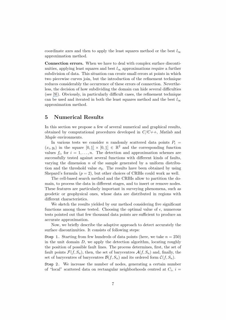
Figure 1 (left) shows that, outside the discontinuities, the function f1(x, y)is constant for x > 0.5, whereas changes enough quickly for x ≤ 0.5, produc-ing a variation of the jump size in Γ1. Moreover, Figure 1 (right) providesthe graphical representation of the least squares curves from the 75 pointsof the set C(f ; Sn). In Figure 2 we show step by step the adaptive de-tection procedure, representing (bottom, from left to right) the subsequentenlarged sets of data points and (top, from left to right) the corresponding

8

sets C(f ; Sn). Precisely, in Figure 2 (A), we report the picture of the pointsbelonging to C(f ; Sn) and obtained by applying the detection procedurefrom 250 scattered data (not represented). Figure 2 (B) and (C) refer tothe sets C(f ; Sn) of the points, obtained by increasing the number of nodeson or close to possible fault lines, as showed in Figure 2 (X) and (Y) re-spectively. Then, Figure 2 (Z) contains the enlarged set of data points fromwhich we get the final set C(f ; Sn) and the relative approximation lines (seeFigure 1 (right)). These are obtained from the last set C(f ; Sn), subdividingit into two subsets.

In the detection phase, to obtain an accurate approximation of the faults,we employ 3479 data points (this number is purely indicative and may varyconsiderably). In some cases, nevertheless, if a rough knowledge of faults(e.g. position, behaviour, etc.) is sufficient, the number of the consideredpoints can be considerably reduced (say, at about a quarter). In doing so,we may reduce the number of steps in the adaptive detection process (seeFigure 2 (B) or (C)), but obviously do not attain the accutacy obtained inthis paper.

All these remarks hold also for the following test functions.

0

0.2

0.4

0.6

0.8

1 0

0.2

0.4

0.6

0.8

10

0.5

1

1.5

2

0 0.1 0.2 0.3 0.4 0.5 0.6 0.7 0.8 0.9 10

0.1

0.2

0.3

0.4

0.5

0.6

0.7

0.8

0.9

1

Figure 1: Test function f1 (left) and least squares approximation curves(right).

Test function 2

The test function [14]

f2(x, y) =

{

0, if x > 0.4, y > 0.4, y < x + 0.2,(x − 1)2 + (y − 1)2, otherwise,

9

0 0.1 0.2 0.3 0.4 0.5 0.6 0.7 0.8 0.9 10

0.1

0.2

0.3

0.4

0.5

0.6

0.7

0.8

0.9

1

(A)

0 0.1 0.2 0.3 0.4 0.5 0.6 0.7 0.8 0.9 10

0.1

0.2

0.3

0.4

0.5

0.6

0.7

0.8

0.9

1

(B)

0 0.1 0.2 0.3 0.4 0.5 0.6 0.7 0.8 0.9 10

0.1

0.2

0.3

0.4

0.5

0.6

0.7

0.8

0.9

1

(C)

0 0.1 0.2 0.3 0.4 0.5 0.6 0.7 0.8 0.9 10

0.1

0.2

0.3

0.4

0.5

0.6

0.7

0.8

0.9

1

(X)

0 0.1 0.2 0.3 0.4 0.5 0.6 0.7 0.8 0.9 10

0.1

0.2

0.3

0.4

0.5

0.6

0.7

0.8

0.9

1

(Y)

0 0.1 0.2 0.3 0.4 0.5 0.6 0.7 0.8 0.9 10

0.1

0.2

0.3

0.4

0.5

0.6

0.7

0.8

0.9

1

(Z)

Figure 2: Output of the adaptive detection procedure for f1.

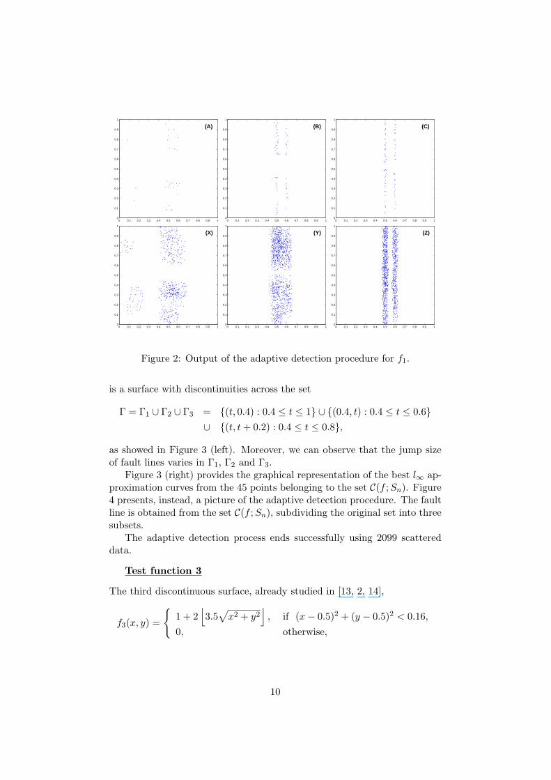
is a surface with discontinuities across the set

Γ = Γ1 ∪ Γ2 ∪ Γ3 = {(t, 0.4) : 0.4 ≤ t ≤ 1} ∪ {(0.4, t) : 0.4 ≤ t ≤ 0.6}

∪ {(t, t + 0.2) : 0.4 ≤ t ≤ 0.8},

as showed in Figure 3 (left). Moreover, we can observe that the jump sizeof fault lines varies in Γ1, Γ2 and Γ3.

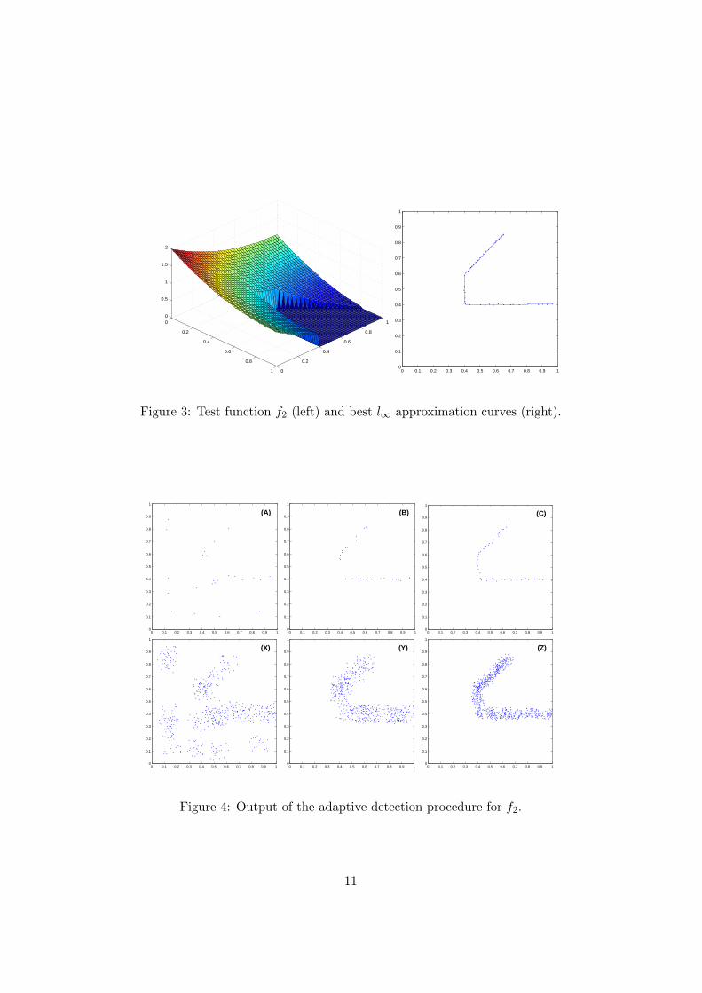
Figure 3 (right) provides the graphical representation of the best l∞ ap-proximation curves from the 45 points belonging to the set C(f ; Sn). Figure4 presents, instead, a picture of the adaptive detection procedure. The faultline is obtained from the set C(f ; Sn), subdividing the original set into threesubsets.

The adaptive detection process ends successfully using 2099 scattereddata.

Test function 3

The third discontinuous surface, already studied in [13, 2, 14],

f3(x, y) =

{

1 + 2⌊

3.5√

x2 + y2⌋

, if (x − 0.5)2 + (y − 0.5)2 < 0.16,

0, otherwise,

10

0

0.2

0.4

0.6

0.8

1 0

0.2

0.4

0.6

0.8

10

0.5

1

1.5

2

0 0.1 0.2 0.3 0.4 0.5 0.6 0.7 0.8 0.9 10

0.1

0.2

0.3

0.4

0.5

0.6

0.7

0.8

0.9

1

Figure 3: Test function f2 (left) and best l∞ approximation curves (right).

0 0.1 0.2 0.3 0.4 0.5 0.6 0.7 0.8 0.9 10

0.1

0.2

0.3

0.4

0.5

0.6

0.7

0.8

0.9

1

(A)

0 0.1 0.2 0.3 0.4 0.5 0.6 0.7 0.8 0.9 10

0.1

0.2

0.3

0.4

0.5

0.6

0.7

0.8

0.9

1

(B)

0 0.1 0.2 0.3 0.4 0.5 0.6 0.7 0.8 0.9 10

0.1

0.2

0.3

0.4

0.5

0.6

0.7

0.8

0.9

1

(C)

0 0.1 0.2 0.3 0.4 0.5 0.6 0.7 0.8 0.9 10

0.1

0.2

0.3

0.4

0.5

0.6

0.7

0.8

0.9

1

(X)

0 0.1 0.2 0.3 0.4 0.5 0.6 0.7 0.8 0.9 10

0.1

0.2

0.3

0.4

0.5

0.6

0.7

0.8

0.9

1

(Y)

0 0.1 0.2 0.3 0.4 0.5 0.6 0.7 0.8 0.9 10

0.1

0.2

0.3

0.4

0.5

0.6

0.7

0.8

0.9

1

(Z)

Figure 4: Output of the adaptive detection procedure for f2.

11

has the discontinuity set given by

Γ = Γ1 ∪ Γ2 ∪ Γ3 = {(x, y) ∈ R2 : (x − 0.5)2 + (y − 0.5)2 = 0.16}

∪ {(x, y) ∈ R2 : x2 + y2 = 16/49, (x − 0.5)2 + (y − 0.5)2 ≤ 0.16}

∪ {(x, y) ∈ R2 : x2 + y2 = 36/49, (x − 0.5)2 + (y − 0.5)2 ≤ 0.16}.

The surface is always constant in D \ Γ.In Figure 5 test function f3(x, y) (left) and graphic obtained by polygo-

nal line method from the ordered 108 points of C(f ; Sn) (right) are shown.Figure 6 presents the results of the adaptive detection procedure. Also inthis case, we consider a subdivision of the set C(f ; Sn). Finally, to obtain agreater smoothness, we apply the refinement technique three times.

In this test, to obtain the result of Figure 5 (right), 5185 nodes areconsidered in input.

00.2

0.40.6

0.81

0

0.2

0.4

0.6

0.8

1

0

1

2

3

4

5

6

7

0 0.1 0.2 0.3 0.4 0.5 0.6 0.7 0.8 0.9 10

0.1

0.2

0.3

0.4

0.5

0.6

0.7

0.8

0.9

1

Figure 5: Test function f3 (left) and polygonal line approximation curves(right).

Test function 4

The next test considers the function (see [16, 2, 14, 15]),

f4(x, y) =

{

(2 − (x − 0.8)2)(2 − (y − 0.8)2), if y > l(x),(1 − (x − 0.5)2)(1 − (y − 0.2)2), otherwise,

with l(x) = 0.5 + 0.2 sin(5πx)/3. The fault set is given by

Γ = {(t, l(t)) : 0 ≤ t ≤ 1}

and its jump size is almost constant on all the domain.Figure 7 contains the test function f4 (left) and the fault approximation

obtained by least squares curve from the 49 points of the set C(f ; Sn) (right),

12

0 0.1 0.2 0.3 0.4 0.5 0.6 0.7 0.8 0.9 10

0.1

0.2

0.3

0.4

0.5

0.6

0.7

0.8

0.9

1

(A)

0 0.1 0.2 0.3 0.4 0.5 0.6 0.7 0.8 0.9 10

0.1

0.2

0.3

0.4

0.5

0.6

0.7

0.8

0.9

1

(B)

0 0.1 0.2 0.3 0.4 0.5 0.6 0.7 0.8 0.9 10

0.1

0.2

0.3

0.4

0.5

0.6

0.7

0.8

0.9

1

(C)

0 0.1 0.2 0.3 0.4 0.5 0.6 0.7 0.8 0.9 10

0.1

0.2

0.3

0.4

0.5

0.6

0.7

0.8

0.9

1

(X)

0 0.1 0.2 0.3 0.4 0.5 0.6 0.7 0.8 0.9 10

0.1

0.2

0.3

0.4

0.5

0.6

0.7

0.8

0.9

1

(Y)

0 0.1 0.2 0.3 0.4 0.5 0.6 0.7 0.8 0.9 10

0.1

0.2

0.3

0.4

0.5

0.6

0.7

0.8

0.9

1

(Z)

Figure 6: Output of the adaptive detection procedure for f3.

while Figure 8 shows step by step the adaptive detection procedure. Splittingup C(f ; Sn) in subsets do not produce considerable advantages.

To end the adaptive process, the number of the employed points is 2705.

Test function 5

Last, we consider the function (see [5])

f5(x, y) =

g(x, y), if y < min(1/3x, 0.25),h(x, y), if min(1/3x, 0.25) ≤ y < 2x − 0.5,6, otherwise,

with

g(x, y) = 1 + 1.4375(

2 − (x − 1)2)

exp(5 (1 − x) (4y − 1)),

h(x, y) = 1 +(

2 − (x − 1)2) (

2 − (y − 1)2)

,

and discontinuity set

Γ = Γ1 ∪ Γ2 =

{(

t,1

3t

)

: 0 ≤ t ≤ 0.75

}

∪

{(

t, 2t −1

2

)

: 0.3 ≤ t ≤ 0.75

}

.

We observe that the jump size of fault line Γ1 vanishes when x tends to 0.75.In Figure 9 we set the test function and the best l∞ approximation

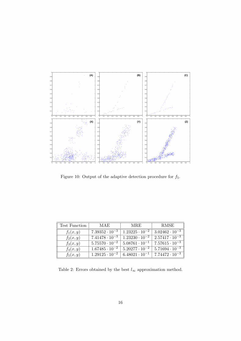
curves derived from the 46 points belonging to C(f ; Sn). Figure 10 shows

13

0

0.2

0.4

0.6

0.8

1 0

0.2

0.4

0.6

0.8

10.5

1

1.5

2

2.5

3

3.5

4

0 0.1 0.2 0.3 0.4 0.5 0.6 0.7 0.8 0.9 10

0.1

0.2

0.3

0.4

0.5

0.6

0.7

0.8

0.9

1

Figure 7: Test function f4 (left) and least squares approximation curve(right).

0 0.1 0.2 0.3 0.4 0.5 0.6 0.7 0.8 0.9 10

0.1

0.2

0.3

0.4

0.5

0.6

0.7

0.8

0.9

1

(A)

0 0.1 0.2 0.3 0.4 0.5 0.6 0.7 0.8 0.9 10

0.1

0.2

0.3

0.4

0.5

0.6

0.7

0.8

0.9

1

(B)

0 0.1 0.2 0.3 0.4 0.5 0.6 0.7 0.8 0.9 10

0.1

0.2

0.3

0.4

0.5

0.6

0.7

0.8

0.9

1

(C)

0 0.1 0.2 0.3 0.4 0.5 0.6 0.7 0.8 0.9 10

0.1

0.2

0.3

0.4

0.5

0.6

0.7

0.8

0.9

1

(X)

0 0.1 0.2 0.3 0.4 0.5 0.6 0.7 0.8 0.9 10

0.1

0.2

0.3

0.4

0.5

0.6

0.7

0.8

0.9

1

(Y)

0 0.1 0.2 0.3 0.4 0.5 0.6 0.7 0.8 0.9 10

0.1

0.2

0.3

0.4

0.5

0.6

0.7

0.8

0.9

1

(Z)

Figure 8: Output of the adaptive detection procedure for f4.

14

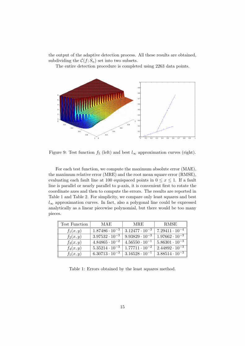
the output of the adaptive detection process. All these results are obtained,subdividing the C(f ; Sn) set into two subsets.

The entire detection procedure is completed using 2263 data points.

0

0.2

0.4

0.6

0.8

1 0

0.2

0.4

0.6

0.8

11

2

3

4

5

6

0 0.1 0.2 0.3 0.4 0.5 0.6 0.7 0.8 0.9 10

0.1

0.2

0.3

0.4

0.5

0.6

0.7

0.8

0.9

1

Figure 9: Test function f5 (left) and best l∞ approximation curves (right).

For each test function, we compute the maximum absolute error (MAE),the maximum relative error (MRE) and the root mean square error (RMSE),evaluating each fault line at 100 equispaced points in 0 ≤ x ≤ 1. If a faultline is parallel or nearly parallel to y-axis, it is convenient first to rotate thecoordinate axes and then to compute the errors. The results are reported inTable 1 and Table 2. For simplicity, we compare only least squares and bestl∞ approximation curves. In fact, also a polygonal line could be expressedanalytically as a linear piecewise polynomial, but there would be too manypieces.

Test Function MAE MRE RMSE

f1(x, y) 1.87486 · 10−3 3.12477 · 10−3 7.29411 · 10−4

f2(x, y) 3.97532 · 10−3 9.93829 · 10−3 1.97662 · 10−3

f3(x, y) 4.84865 · 10−2 4.56550 · 10−1 5.86301 · 10−3

f4(x, y) 5.35214 · 10−3 1.77711 · 10−2 2.44892 · 10−3

f5(x, y) 6.30713 · 10−3 3.16528 · 10−1 3.88514 · 10−3

Table 1: Errors obtained by the least squares method.

15

0 0.1 0.2 0.3 0.4 0.5 0.6 0.7 0.8 0.9 10

0.1

0.2

0.3

0.4

0.5

0.6

0.7

0.8

0.9

1

(A)

0 0.1 0.2 0.3 0.4 0.5 0.6 0.7 0.8 0.9 10

0.1

0.2

0.3

0.4

0.5

0.6

0.7

0.8

0.9

1

(B)

0 0.1 0.2 0.3 0.4 0.5 0.6 0.7 0.8 0.9 10

0.1

0.2

0.3

0.4

0.5

0.6

0.7

0.8

0.9

1

(C)

0 0.1 0.2 0.3 0.4 0.5 0.6 0.7 0.8 0.9 10

0.1

0.2

0.3

0.4

0.5

0.6

0.7

0.8

0.9

1

(X)

0 0.1 0.2 0.3 0.4 0.5 0.6 0.7 0.8 0.9 10

0.1

0.2

0.3

0.4

0.5

0.6

0.7

0.8

0.9

1

(Y)

0 0.1 0.2 0.3 0.4 0.5 0.6 0.7 0.8 0.9 10

0.1

0.2

0.3

0.4

0.5

0.6

0.7

0.8

0.9

1

(Z)

Figure 10: Output of the adaptive detection procedure for f5.

Test Function MAE MRE RMSE

f1(x, y) 7.39352 · 10−3 1.23225 · 10−2 3.02462 · 10−3

f2(x, y) 7.41478 · 10−3 1.23230 · 10−2 2.57417 · 10−3

f3(x, y) 5.75570 · 10−2 5.08761 · 10−1 7.57615 · 10−3

f4(x, y) 1.67485 · 10−2 5.20277 · 10−2 5.71694 · 10−3

f5(x, y) 1.29125 · 10−2 6.48021 · 10−1 7.74472 · 10−3

Table 2: Errors obtained by the best l∞ approximation method.

16

6 Final Remarks

In this paper, we have presented a method for the adaptive detection andapproximation of fault lines in a discontinuous surface from scattered data.The approach we propose ensures good results, although the number of datapoints is meaningfully reduced. Indeed, in some applications, the searchof information (data) is very expensive, so that a reduction of cost is aremarkable goal.

In our analysis, we suppose that the considered surface is smooth outsidefaults. If this does not happen, then the detection algorithm may identifyfalse fault points. If the jump size varies rather fastly or vanishes, it followsthat the optimal choice of a global threshold parameter σ0 is an essentialtask. In future, a possible development could consist in splitting up thedomain in a uniform grid and find a (local) threshold parameter for eachgrid cell. This idea should allow us to localize only the actual points ofdiscontinuity, reducing the possibility of finding false fault points. However,it is yet an open problem and we are considering it.

Finally, we have tested the possibility to use a variable and adaptive gridin the cell-based search method, but the results have not showed meaningfuladvantages.

References

[1] Allasia, G., Cardinal basis interpolation on multivariate scattered data,Nonlinear Analysis Forum 6 (1) (2001), 1–13.

[2] Allasia, G., R. Besenghi, and A. De Rossi, A scattered data approxi-mation scheme for the detection of fault lines, in T. Lyche, and L.L.Schumaker (eds.), Mathematical methods for curves and surfaces: Oslo2000, Vanderbilt Univ. Press., Nashville TN, 2001, 25–34.

[3] Allasia, G., R. Besenghi, and R. Cavoretto, Accurate approximation ofunknown fault lines from scattered data, submitted paper.

[4] Arcangeli, R., M.C. Lopez de Silanes, and J.J. Torrens, Multidimen-sional minimizing splines. Theory and applications. Kluwer, Boston,MA, 2004.

[5] Arge, E., and M. Floater, Approximating scattered data with disconti-nuities, Numer. Algorithms 8 (1994), 149–166.

[6] Bentley, J.L., and J.H. Friedman, Data structures for range searching,Comput. Surveys 11 (1979), 397–409.

[7] Besenghi, R., and G. Allasia, Scattered data near-interpolation withapplication to discontinuous surfaces, in A. Cohen, C. Rabut, and L.L.

17

Schumaker (eds.), Curves and surfaces fitting: Saint-Malo 1999, Van-derbilt Univ. Press., Nashville TN, 2000, 75–84.

[8] Besenghi, R., M. Costanzo, and A. De Rossi, A parallel algorithm formodelling faulted surfaces from scattered data, Int. J. Comput. Numer.Anal. Appl. 3 (2003), 419–438.

[9] Crampton, A., and J.C. Mason, Detecting and approximating fault linesfrom randomly scattered data, Numer. Algorithms 39 (2005), 115–130.

[10] Fremming, N.P., Ø. Hjelle, and C. Tarrou, Surface modelling from scat-tered geological data, in M. Dæhlem, and A. Tveito (eds.), Numeri-cal methods and software tools in industrial mathematics, Birkhauser,Boston, 1997, 301–315.

[11] Gout, C., and C. Le Guyader, Segmentation of complex geophysicalstructures with well data, Comput. Geosci. 10 (2006), 361–372.

[12] Gout, C., C. Le Guyader, L. Romani, and A.G. Saint-Guirons, Approx-imation of surfaces with fault(s) and/or rapidly varying data, using asegmentation process, Dm-splines and the finite element method, Nu-mer. Algorithms 48 (2008), 67–92.

[13] Gutzmer, T., and A. Iske, Detection of discontinuities in scattered dataapproximation, Numer. Algorithms 16 (1997), 155–170.

[14] Lopez de Silanes, M.C., M.C. Parra, and J.J. Torrens, Vertical andoblique fault detection in explicit surfaces, J. Comput. Appl. Math.140 (2002), 559–585.

[15] Lopez de Silanes, M.C., M.C. Parra, and J.J. Torrens, On a new char-acterization of finite jump discontinuities and its application to verticalfault detection, Math. Comput. Simul. 77 (2008), 247–256.

[16] Parra, M.C., M.C. Lopez de Silanes, and J.J. Torrens, Vertical faultdetection from scattered data, J. Comput. Appl. Math. 73 (1996), 225–239.

18