Modeling Strong Discontinuities using Generalized Finite Element

Method (GFEM)

Mahendra Kumar Pal

A Dissertation Submitted to

Indian Institute of Technology Hyderabad

In Partial Fulfillment of the Requirements for

The Degree of Master of Technology

Department of Civil Engineering

Indian Institute of Technology Hyderabad

June, 2012

ii

Declaration

I declare that this written submission represents my ideas in my own words, and

where others ideas or words have been included. I have adequately cited and

referenced the original sources. I also declare that I have adhered to all principles of

academic honesty and integrity and have not misrepresented or fabricated or

falsified any idea/data/fact/source in my submission. I understand that any violation

of the above will be a cause for disciplinary action by the Institute and can also

evoke penal action from the sources that have thus not been properly cited, or from

whom proper permission has not been taken when needed.

(Signature)

Mahendra Kumar Pal

(----- Student Name --)

CE10M06

(---Roll No--)

iii

iv

Acknowledgements

I would like to praise and thanks to almighty GOD for his gift to me as wisdom and

knowledge. He conferred the intelligence to me for endeavoring in my research

work.

I would like to convey my special thanks to my thesis advisor Dr. A. Rajagopal for

all his faith and confidence in me. He believed in me and given such an awesome

topic to work on it. Working with him and being a part of his research group is

privilege for me. It would have been highly impossible for me to move forward

without his motivation and well organized guidance. His encouragement and

technical guidance made my thesis work worth full and interesting. I can never

repay the valuable time that he had devoted to me during my thesis work. Working

with him was indeed a fantastic, fruitful, and an unforgettable experience of my life.

I am also indebted to say my heartily thanks to my Head of Department, Prof.

K.V.L.Subraminam for the confidence in me that he always shown. It gives me

immense pleasure to thank my faculty members who taught during my M.Tech

course work. I would like to thank Prof. M.R. Madhav, Dr. B. Umashakar, Dr. S.

Sireesh for their valuable suggestion during my course work.

I am thankful to my prestigious institute Indian Institute of Technology, Hyderabad

for all the support and providing everything whatever was required for my research

work.

I am grateful and thankful all my friends. I would like to say special thanks to my

supervisor’s research group members L. Harish (M. Tech.), B.Umesh (PhD.),

Balakrishana (PhD.), Nitin Kumar (M.Tech.), KS.Balaji (M.Tech.), S. Madhukar

(Project Associate).

v

I would like to thank to all my classmates of Civil Engineering. I am indebted to all

resident students of the 600 series of IIT Hyderabad hostel. I would like to extend

my huge thanks to Pruthiviraj Chavan, Tinkle Chugh, Ravi Selgar, Mohit Joshi,

Vikrant Veerkar, Amit Dhige, G.Sahith, Pankaj Sahlot, JaiMohan Srivastava,

Abhishek Gupta, M. Nagarjuna, P. Naidu, Pankaj Jha, Md. Kasafdooja and all others

for their friendship and encouragement. I admire their helping nature.

Last but not the least, I owe a great deal of appreciation to my father and mother

who gifted me this life. I will not forget to say thanks a lot to my lovely and

sweetest sister Priyanka for all her faith and believe in me. I owe everything to her.

I would like to say special thanks to several peoples, who have knowingly

unknowingly helped me in the completion of this project.

vi

Dedicated to

My parents and my sweetest sister

vii

Abstract

Computational modeling of strong discontinuities is a challenging a task. Stress

analysis and shape sensitivity can be done with any simulation method such as finite

element method, finite difference method, Rayleigh-Ritz method, weighted residual

method or least square method. All these numerical analysis methods are

computationally expensive and uneconomical. Mesh dependency with respect to

fracture boundary is a major problem in these methods. Furthermore accuracy of the

methods depends on the size of the discretized element.

To bring the mesh independency the classical FE approximation is extended or

enriched. This enrichment gives a higher order approximation and better

reproducibility of the field ahead of the crack tip. The developed method requires a

very less computation space and is also an economical method for complex

problems. This proposed method is called as extended finite element merthod

(XFEM).

The Generalized Finite Element Method (GFEM) is based on the enrichment of the

classical approximation. The enriched basis is achieved with the help of the various

enrichment functions. These enrichment functions are capable to mimic the presence

of the crack boundary, dislocation or discontinuity in the domain. These functions

are selected on a priori knowledge of the solution of the given problem. Different

enriched basis function has been demonstrated for demonstrating the capability of

the GFEM.

In the present work GFEM is presented as a potential methodology for modeling the

complex geometries and fracture problems. Methodology is implemented to assess

the true strength, durability and the integrity of the structure/ structural components.

The interdependency of the input variables and their effect on the output has been

studied in the sensitivity analysis. During the implementation of the methodology

various issues like inter-boundary conflict for the different approximations,

numerical integration of the crack domain, assembly of the global stiffness matrix,

viii

and numerical instability of the global stiffness matrix have been suitably addressed.

These issues have been explored and rectified with efficient and optimal method.

Structural optimization plays the key role in the design industry. Prediction of the

fatigue life and strength of the structure is another important factor of this industry.

Fatigue life and the strength depend on the various independent and dependent

variables. It's a challenging task to identify the important variable in the design.

This objective can be easily achieved with the shape sensitivity analysis of the any

fracture parameter such as stress intensity factor (SIF), J-integral. We have studied

the shape sensitivity of the J-integral. Results show the dependency of the J-integral

on the various conditions as well as on variables.

In order to demonstrate the potential of the method, an edge crack problem has been

considered an example. Elastic and hyper-elastic cases are considered for analysis.

Sensitivity analysis has been illustrated for same geometry numerical problem.

Sensitivity analysis has been performed with different boundary and loading

conditions. Effect of crack length on the J-integral has been illustrated. The

sensitivity analysis is based on the variational formulation of the continuum

mechanics. A bimaterial domain has been also taken as another example for

sensitivity analysis. Mathematically sensitivity analysis is defined as the

differentiation of that entity with respect to the independent variable. This definition

has been used for validation of the results. This alternative approach is based on the

first principle of the differentiation.

ix

Nomenclature

Ni Classical shape function

Enrichment function

Derivative of enrichment function

i Classical Nodal freedom

Additional Nodal freedom

Heaviside function

and Polar coordinate system near the tip

Traction Boundary

Displacement Boundary

Cracked Boundary

1st order stress tensor

Body force

Applied Traction

Prescribed Displacement

Ω Domain

Work done and strain energy

Shape function derivative matrix

Stiffness matrix

Vector of element external force

Stress intensity factor for Mode-I

Stress intensity factor for Mode-II

Stress intensity factor for Mode-III

J-Integral

Distance function

Blending function

and Lame’s parameters

and First and second invariant of the unimodular component of the left Cauchy-

Green Deformation tensor

x

Material response tensor of 4th order

Material response tensor of 2nd order

Transformation mapping

Velocity field

Material derivative of displacement field

Material derivative of J-Integral

Sensitivity function

Sensitivity function

Young’s Modulas

Bulk Modulas

δ Prescribed displacement

Length* width

xi

Contents

Declaration .......................................................................................................................... ii

Approval Sheet ................................................................. Error! Bookmark not defined.

Acknowledgements............................................................................................................ iv

Abstract ............................................................................................................................. vii

Nomenclature ........................................................................................................... ix

1 Introduction

1.1 Motivation ................................................................................................................. 1

1.3 Outline of thesis ........................................................................................................ 2

2 Literature review……………………………………………………………………………………..3

3 Fracture Mechanics: A Review

3.1 Basics of fracture mechanics .................................................................................. 12

3.2 Mode of Failure ...................................................................................................... 13

3.3 Stress Intensity factor .............................................................................................. 14

3.4 J-Integral ................................................................................................................. 18

4 Generalized Finite Element Method

4.1 Introduction ............................................................................................................. 20

4.2 Realization of enrichment function in 1-D ............................................................. 20

4.2.1 Partition of Unity ............................................................................................. 21

4.2.2 Heaviside Function ......................................................................................... 22

4.2.3 Modified Heaviside Function ......................................................................... 23

4.3 Realization of enrichment function in 2-D .................................................................

4.3.1 Modified Heaviside Function ......................................................................... 25

4.3.2 Crack tip enrichment Function ....................................................................... 27

4.3.3 Level Set enrichment function ........................................................................ 28

4.4 Conclusion .............................................................................................................. 31

xii

5 Blending Element

5.1 Introduction ............................................................................................................. 32

5.2 Problem Statement .................................................................................................. 32

5.3 Literature review ..................................................................................................... 33

5.4 Classification of element ........................................................................................ 33

5.5 Characterstics of Blending function ........................................................................ 34

5.6 Properties of Blending function .............................................................................. 34

5.7 Examples of Blending function .............................................................................. 35

5.8 Blending function used in thesis ............................................................................. 37

5.9 Conclusion .............................................................................................................. 37

6. Galerkin Formulation ........................................................................................38

7 Numerical Example: Stress analysis and SIF study

7.1 Problem Defintion ................................................................................................... 47

7.2 Modeling 2-D edge crack problem ........................................................................ 47

7.2.1 Elastic Analysis ............................................................................................... 48

7.2.2 Hyperelastic Analysis ...................................................................................... 49

7.3 Modeling 2-D inclined crack problem ................................................................... 52

7.3.1 Elastic Analysis ............................................................................................... 52

7.4 Conclusion .............................................................................................................. 53

8 Sensitivity Analysis

8.1 Introduction ............................................................................................................. 54

8.2 Literature Survey .................................................................................................. 54

8.3 Velocity Field ....................................................................................................... 55

8.4 Sensitivity Analysis .............................................................................................. 57

8.4.1 Material derivative........................................................................................... 57

8.4.2 Variational formulation ................................................................................... 57

8.4.3 Sensitivity analysis of J-Integral ..................................................................... 58

8.4.4 Flow Chart ....................................................................................................... 60

8.4.5 Numerical Example: Problem Definition ........................................................ 61

8.4.6 Result and Discussion...................................................................................... 63

xiii

8 Conlusion ...............................................................................................................66

8 List of Figures .......................................................................................................68

9 List of Tables .........................................................................................................70

10 Appendix

14.1 Appendix -I: g function for sensitivity analysis .................................................. 71

14.2 Appendix -II: G function for Sensitivity analysis ............................................... 72

14.3 Appendix -III: Strcuture of the MATLAB Code ................................................ 73

References .................................................................................................................78

1

Chapter 1

Introduction

1.1 Motivation

The Finite Element Method (FEM) has been found wide used of enormous application in

many fields. FEM approximation is interpolatory in nature. This interpolatory nature of

approximation in FEM makes the solution mesh dependent. One possibility to achieve

accuracy in solution is by adaptive refinement of mesh. However such schemes are

computationally expensive. FEM does not suit well to treat problems with discontinuities

(i.e. Crack propogation) that do not align with the mesh. Meshless Methods (MMs) have

been used with objective of eliminating part of difficulties associated with reliance on

mesh to construct the approximation. MMs are based on approximations that are not

interplatory in nature but are based on alternative strategies like for instance the moving

least square (MLS) approach. The problem associated with these methods is that they are

computationally expensive and non interpolatory nature requires Lagrange multipliers for

imposition of boundary conditions.

There has been a need for developing better approximation schemes that have

interpolatory characteristics, consistency and stability. Also in using such methods for

fracture problems, the methods should be capable of reproducing the actual stress/ strain

field ahead of the crack tip. To this end, there has been many works on improving the

classical FEM approximations and one such methodology was coined as Extended Finite

Element Methods (XFEM). In these methods the approximation is enriched by some

additional enrichment functions. However there were difficulties associated with the

method as regards making appropriate choice on the enrichment functions.

Minimizing the error between approximation solution and exact solution can make

appropriate choice on the enrichment functions belonging to a particular function space.

Proper Orthogonal Decomposition (POD) is done on the fact that distance between

member of ensemble and subspace is minimal. An XFEM with choice on enrichment

functions based on POD is termed as Generalized Finite Element Method (GFEM) [10].

2

In this work POD has been used for finding out the enrichment basis function for GFEM

approximation [10]. Such a enrichment function accounts for the oscillatory nature of the

solution ahead of singular regions. The global approximation has been constructed by

combining the local bases with partition of unity functions (i.e. classical basis function).

1.2 Outline of Thesis

The thesis has been divided into the 9 chapters. The first chapter contains the motivation and

second chapter contains the literature survey of XFEM/GFEM. Third chapter contains the review

of fracture mechanics. Realization of the capability of GFEM has been illustrated through the

shape functions in 1-D and 2-D in the following chapter. Different examples of enrichment

functions have been demonstrated in this chapter. Two scales GFEM has two different orders of

the approximation, which results into the inter-boundary conflict for the neighboring elements to

enriched elements. The blending element concept has been introduced to ensure the continuity

among the two different approximations. Next chapter continues the discussion about the

blending element. Fourth chapter contains the mathematical foundation of Galerkin formulation

of the GFEM and the numerical integration schemes respectively. This chapter also contains the

discussion over the implementation issues of the GFEM. Stress analysis of the fracture problems

has been shown in the seventh chapter. Eighth chapter contains the sensitivity analysis of the edge

crack problem. Final chapter ends with a conclusion and the Scope of the future work.

3

Chapter 2

Literature Review

2.1 Choice of Enrichment Function in XFEM/GFEM

A Judicious choice is required to be made in the selection of enrichment function. The main

objective of enrichment function is that it should able to reproduce the singular stress field near

crack tip. Selection of enrichment function is done by apriori knowledge of solution. XFEM and

meshless methods have used the partition of unity enrichment for solving the crack problems.

Belytschko et al. [7] described methods based on the partition of unity for approximating

discontinuous functions in finite element and meshless formulations. Fries and Belytschko [8]

presented a new intrinsic enrichment method for treating arbitrary discontinuities in a FEM

context. Unlike the standard XFEM, no additional unknowns were introduced at the nodes whose

supports were crossed by discontinuities. An approximation space was constructed consisting of

mesh based, enriched moving least squares (MLS) functions near discontinuities and standard FE

shape functions elsewhere. Belytschko and Black [1] introduced a method for solving crack

problem in finite element framework. In this method the meshing task is reduced by enriching the

element near the crack tip and along the crack face with leading singular crack tip asymptotic

displacement fields using partition of unity method to account for the presence of crack.

Enrichment function need not be known solely in closed framework but results from numerical

simulation can be used as enrichment functions. Later authors used canonical domain containing

features such as branched cracks, or closely spaced voids to generate what they called mesh-based

handbook functions. This approach is very useful for the situations in which analytical

expressions, which reflect the nature of solutions, are not available. For enrichment in the

introduction paper of GFEM, Strouboulis [4] had used harmonic function as enrichment function

to enrich the basis of approximation. Aquino et al [10] had shown that due to appealing

approximation properties, POD modes are best choice of the enrichment function in the GEFM.

For a proper orthogonal decomposition – Generalized finite element method (POD-GFEM)

formulation, the POD modes (x) are used as the enrichment functions in Equation (1). GFEM

basis function is union of the classical finite element polynomial basis { }

, and the enriched

4

bases, { } where is number of nodes and is the enrichment

functions (POD modes). This has been used in the present work

∑ ∑ ∑ (2.1)

Where is the enrichment function, is total number of nodes, is the additional

degrees of freedoms.

Mousavi et al [9] had proposed new enrichment function named as harmonic enrichment function.

To model weak discontinuities in bimaterial interfaces, Moes et.al [11] proposed a ridge function.

The ridge function is continuous across the interface, though the gradient of ridge function is

discontinuous. The ridge enrichment is well suited for continuous deformation map and Moes et

al [11] reported optimally convergent results in the small strain regime for linear elastic materials

with relatively small modulus mismatch. Arndtl et al [12] had used generalized finite element

method for vibration analysis of straight bars and trusses. They had used enrichment functions as

combination of some trigonometric functions.

Along with selection of enrichment function, there are some issues, which appear in the

evaluation of integrals over the element domain. Classical Gauss quadrature rules fails for

discontinuous domain. Ventura [13] had shown the way that how classical gauss quadrature rule

can be used for discontinuous domain by splitting the element into sub cells. Sunderrajan et. al

[26] had proposed the numerical integration scheme based on conformal mapping. Convergence

is main criterion to be satisfied for any kind of method. Labordr et al [14] and Chahine et al [15]

has targeted the convergence and studied the convergence for variety of XFEM on cracked

domain.

Numerical instability is a problem concerning solution in GFEM. These numerical instabilities

come into the scenes due to the singular stress field ahead of crack tip. Peter and Hack [16] had

discussed the ways that a singular stiffness matrix may be avoided by static condensation of row

and column corresponding to some of the enhanced degree of freedoms. Xiao and Karihaloo [17]

discussed improving the accuracy of XFEM crack tip fields using higher order quadrature and

static admissible stress recovery procedures. The static admissible stress recovery scheme is

constructed by the basis functions and Moving Least Square (MLS) to interpolate the stress at

integration points obtained by XFEM.

XFEM has been widely used in field of multiscale modeling of the material. In multiscale

modeling different level of accuracy is required which varies from atomic level to macro

simulation level. Since GFEM approximation has ability to reproduce multiscale effects in

modeling so many of the researchers have used GFEM technique for multiscale modeling. Hirari

et. al [18] had proposed zooming technique with local global approximation which enhance the

classical FEM over the entire region of domain. In this technique mesh was refined on the critical

region (i.e. stress concentration region). In a superposition multiscale approach, global and local

5

parts are modeled independently, and then superimposed to provide the final solution by

satisfying the compatibility equations. Haider et. al [19] has proposed homogenization based

multiscale modeling which is based on domain decomposition technique. In this technique

domain is divided into several sub domains, which are connected by the interface element.

2.2 Review of XFEM applications

Many of the engineering problems had been analyzed using the XFEM. A few of them has been

discussed here. The methodology for multiple and arbitrary crack propagation problem had been

proposed by Areias and Belytschko [20] with enrichment of rotation field. Areiase et. al [21] had

proposed the very similar formulation as Hansbo and Hansbo [22] did for the evolution of crack

in thin shells using mid surface displacement and director field discontinuities.

XFEM has been explored for dynamic problems by Belytschko et. al [23], Belytschko and Chen

[24], and Zi et. al [25] which are based on singular enrichment FEM. Rathore et. al [26] proposed

GFEM to model dynamic fracture with incorporating time dependency. Menouilllard et. al [27]

published a paper on explicit XFEM. In this publication they have introduced lumped mass matrix

for enriched element.

XFEM has been wide application for coupled problems. Chessa and Belytschko [28, 29]

published and proposed a methodology for solving hyperbolic problems with discontinuities

based on a locally enriched space–time XFEM. The coupling was implemented through a weak

enforcement of the continuity of the flux between the space–time and semi-discrete domains in a

manner similar to discontinuous Galerkin methods. Furthermore Rathoré et al. [30] proposed a

combined space–time XFEM, based on the idea of the time extended finite element method,

allowing a suitable form of the time stepping formulae to study the stability and energy

conservation.

The feasibility of extending the traditional FEM to Generalized finite element method (GFEM)

has been demonstrated by Strouboulis and Babuska [3]. The target had been achieved by adding

special functions to the approximation. These special functions can be selected on the basis of

available information about boundary value problems. The functions are combined with linear

finite element hat functions, which follow the partition of unity and provide the flexibility in the

approximation. The flexibility of GFEM means approximation space can be formed by any

mixture of special local approximation functions at disposal. One can mix quadratic and higher

order traditional polynomial basis function defined on master element. Strouboulis et. al [3] have

chosen grids which are quasi uniform meshes typically used in standard FEM and used the regular

Legendre shape functions with element degree two. He has assumed two combinations of special

functions. In the first case, he starts with the uniform p-order tradition FEM shape functions

pFEM=2 and add one or more layer of singular function. This is called singular case. In second case

he computed approximation in which he limits the FEM element degree to pFEM=1 and added

6

successive terms. Using successive increasing terms in all special functions may give error

comparable but no significant advantage in convergence is obtained beyond that provided by

singular path space. This is because he used the singular patch only in the elements with vertex at

the corner, if he may have increase the n layer i.e. use of special singular functions at vertices

surrounding the corner, he may get a good convergence rate. In this study they have focused on

the theory behind the new approximation and it was limited to the 2-dimensional problems.

At the same time Duarte et. al [5] had explored the same concept for three dimensional problems.

Their works based on traditional h-p finite element method. They had used tetrahedral mesh and a

priori knowledge of elastic solution to get the p-orthotropic approximation. They have improved

the traditional h-p finite element method by using h adaptivity with the partition of unity. They

had suggested using a polynomial basis function to build the approximation space. They had

investigated the structure of stiffness matrix for its rank and size of matrix. They have calculated

the strain energy and showed the applicability of the proposed algorithm.

After establishing the theoretical foundation of GFEM, Strouboulis et. al [4] had elaborated the it

for the various applications. GFEM is mesh independent methodology and is based on optimal

basis function.

During implementation they came up with some issues. The main issue in the GFEM came out as

the integration as a classical Gaussian quadrature rule fails due to the presence of discontinuity.

So to avoid this shortcoming, they had proposed the fast remeshing approach. In this approach

they had divided the element into subdivision and named it as nested subdivision. This algorithm

became the most essential tool for implementation of GFEM in fracture problem.

Second issue appeared as the decision on the selection of enrichment functions since Shape

function of any methodology reflects the behavior of its approximation. Babuska et. al [31] had

taken this issue and explained the principle for the selection of enrichment function. They had

illustrated the performance of various kinds of enrichment function such as a sine function,

polynomial function and other trigonometric functions. They have made remarks on the order of

the function through the asymptotic rate of convergence. They had illustrated the polynomial

function by pre-asymptotic performance of approximation. They had concluded that shape

functions are best available information about the approximation method. They had made remarks

that enrichment function should characterize on the smoothness. In case of sobolev- type spaces

the polynomial function is the best choice. They emphasized on the compact support ness of the

basis function.

Another issue was realized as the inter-boundary approximation conflict. There is a jump between

the enrichment approximation and classical approximation. Due to this jump between two

approximations, there is degradation in the convergence rate. For increasing the computational

efficiency blending function had been used for smoothing the approximation. This concept was

introduced by Sukumar [52] and then it has been elaborated by Chessa et. al [32]. They had

7

introduced the enhanced strain methods, which is basically depends on the eliminating the

unwanted terms in the approximation. They had assumed the strain as a summation of symmetric

displacement gradient and an enhanced strain filed.

Where is strain, is displacement gradient

They had put the condition for discontinuous polynomial enrichment that blending element will

give linear field if the following inequality holds.

Where complete order of the function, order of the shape function, order of the polynomial

enrichment function.

Performance of the developed tool can be increased either using the strain enhanced element for

blending element or by using signed function with polynomial functions.

Babuska et. al [33] had presented the state of the art of GFEM as a review paper. In this paper

they had briefly discussed about the main ideas, and various issues related to the GFEM. They

had documented the mathematical foundation and the formulation of GFEM approximation. They

have talked about the selection of the approximation spaces. Selection of the approximation

function depends upon the following points

Available information on the elastic solution in terms of Sobolev spaces and boundary value

problem is used for obtaining the enrichment function. Using these enrichment functions, they are

making the decision for the order of the approximation. The decision for the selection of

enrichment function also depends on the a priori knowledge of the solution. This decision is taken

with preserving the conformal mapping of the complex geometries.

They have emphasized on the implementation portion of the GFEM and the issue related to the

implementation. Finally they have concluded that GFEM is the best tool for problems with

complex geometries and non-smooth solution. GFEM has potential of being used in context of

mixed formulation.

Pereira et. al [34] has implemented the contour integral method to extract the SIF values from

GFEM solutions. They had investigated the contour integral method, cutoff function method

along with J-integral method for calculating the SIF values. They have studied the relative error

variation with respect to the number of degrees of freedom, integration radius. Variation of SIF

values ( and ) with respect to the number of degrees of freedom and integration radius had

been demonstrated. They have made remarks that these parameters are sensitive to the extraction

domain. Selection of extraction domain is an important decision in this method.

Realizing the potential of GFEM, Strouboulis et. al [35] has extended their work for solving the

Helmholtz equation. In the proposed methodology they have used the plane wave function as the

enrichment function. They have studied the pollution effects in the results. Pollution effects can

(2.2)

(2.3)

8

be defined as the deviation of Galerkin solution from the exact solution. They had studied the

and convergence. is the number of plane waves added. They had talked about the

implementation of the proposed methodology. Error follows the triangle’s inequality

|‖|

|‖ ‖|

|‖| ‖|

|‖ ‖|

|‖ ‖|

|‖

‖|

|‖ is the numerical integration error. They had used Gauss elimination with partial

pivoting for solving the discrete system of equations. They had studied the relative error with

respect to the number of degrees of freedom. It was observed that the pollution effect cannot be

avoided and Convergence criterion has an exponential rate with respect to wave direction.

Numerical integration is an important step in GFEM. One has to very careful in the calculation of

the same.

In another work [36] choice of enrichment function and various kinds of errors are discussed in

the solution. Pollution errors are directly dependent on the number of plane wave functions.

Choice of handbook function affects the convergence of the approximation. But the choice of

such function depends on the computation cost and ease of implementation. It does not affect

convergence. Boundary conditions can also affect the accuracy of the solution, since they can

couple with error from interior approximation and other dominant computing the errors. In this

work they have studied the relative error with respect to the number of plane waves used in

solving the system.

Duarte et.al [37] has an emphasized on the application of global –local enrichment function in 3-

D fracture, which has been successfully used to construct an enriched basis for generalized FEM.

Global-local enrichment function uses the same approach as used in global-local FEM.

Fundamental difference, however, is that the proposed generalized FEM accounts for possible

interaction of local (near crack for example) and global (structural) behavior. These interactions

can be accounted when solving the global problem with global local enrichment functions. This is

in contrast to standard global-local FEM.

This global-local enrichment approach is used to define following vector-valued global shape

function

locu

Where denotes a global partition of unity function. This function is used at nodes xα of the

global mesh whose support, is contained in the local domain .

Let’s denotes generalized FEM approximation of the solution of governing differential

equation. The approximation is solution of following problem

(2.4)

(2.5)

9

Find )(h)( 1hp0

GGGG Xu such that,

)(h

G

p

G

o

G Xv

,...)(:)( dsvudsvtdsvudxvu o

G

o

G

o

G

o

G

o

G

o

G

GGGG

where

is a discretization of the Hilbert space defined on , built with

generalized FEM shape function and is a penalty parameter

Srinivasan et. al [38] have presented the extension GFEM in the context of heterogeneous

material. They have done hyperelastic analysis of bimaterial solid. In the proposed methodology,

they have considered the approximation function as the summation of the classical and enriched

displacement fields. They have considered the independent enrichment functions, which are

decided on the basis of a priori knowledge of the solution field. These enrichment functions are

linearly independent of each other.

∑ ∑ ∑

For demonstrating the proposed methodology, they have used Ridge function in place of classical

Heaviside function. They have demonstrated the capability and robustness of the discontinuous

deformation map formulation. Belytschko et. al [39] has presented a review paper entitled as A

review of XFEM/GFEM for material modeling. In this publication they have mentioned about the

capabilities and advances of the GFEM.

They had discussed the various kinds of the enrichment function. As the selection of the

enrichment function depends on the priori knowledge of the solution. They have mentioned type

of enrichment function depending on the type of the problem definition. These are tabulated in

Table 1.

Table 2.1: Type of enrichment function and their use

S.No. Type of Problem Enrichment function

1

Crack / Fracture

Problem

Heaviside function for crack +Level set function

Crack- tip enrichment function for tip

Level set function

2

Dislocation

Level set function

Combined step and core enrichment function

Step enrichment functions- for non-linear and anisotropic

problem.

3 Grain Boundaries Heaviside step function

4

Phase interface

Gradient of approximation function

Ridge function or Tent function

Signed distance function

(2.6)

(2.7)

10

In the current state of construction, our structures are becoming taller and taller. These taller

structures are dynamically unstable. They may have vibration and other oscillation. Reason for

these kinds of effects may be wind or earthquake force. Even water current force can also be a

reason in the case of bridge pillar. Vibration analysis of such kind of structures is very tough and

complicated to the implementation point of view. Arndt et. al [40] had illustrated the vibration

analysis of the these kinds of tall structures. They had demonstrated the proposed methodology

for a straight bar and trusses. In the study they have assumed the approximation function as a

summation of classical approximation and the enriched approximation.

∑ ∑

[∑

]

is the classical shape function, and are enrichment functions.

The enrichment functions for vibration analysis are as follows

( )

( )

( )

( )

Babuska et. al [41] had extended the GFEM work form fracture simulation to multiscale

modeling. This work was done with the objective of optimal accuracy. An approximation error

had been controlled with the help of local approximation. They had talked about the identifying

the local approximation spaces. Then the optimal local approximation space is combined within

the GFEM. These optimal local spaces have been used as the enrichment functions. The next

question arises that how to find out the optimal local spaces. They had done some mathematically

manipulations and shown that this is like an eigenvalue problem. Finding out the eigenvalues and

corresponding eigenvector is an easy from an implementation point of view. Eigenvalues and

corresponding vector can be found out using Singular value decomposition (SVD), Proper

Orthogonal Decomposition (POD) or eigen value problem itself. They have developed a

mathematical formulation for the homogenization problem. As an example they had considered

the fiber reinforced composites, which is a typical example for multiscale modeling. They had

discussed the associated approximation error.

(2.8 a)

(2.8 b)

(2.9)

11

2.3 Observations from literature review

Selection of these enrichment functions is still a challenging work which is usually done with the

priori knowledge of solution. Here in this work we are using POD [10] basis function as

enrichment function for our case. These basis functions can also be readily used for multiscale

modeling. Numerical Integration is another challenging work to incorporate within the

formulation. It’s essential to use a very efficient and versatile integration scheme for evaluation of

integrals over discontinuous domain. In this work we adopt an element partition method [13] for

numerical evaluation of integrals. Blending element approximation is one more crucial deciding

factor to be considered. For bringing the smoothness of approximation function over the all nodes

of blending element, blending or ramp function has been used.

2.4 Objective and Scope of the Work

[1] To perform a state of the art review on XFEM/GFEM technique

[2] To study and incorporate various types of enrichment functions that will be helpful in

developing enriched bilinear quadrilateral elements.

[3] To develop software for two scale modeling of strong discontinuities using GFEM

that will be mesh independent and require no remeshing. The software will

incorporate suitable quadrature scheme for numerical evaluation of integrals for each

element.

[4] To demonstrate the working of the software through numerical experiments.

[5] To demonstrate the sensitivity analysis of the edge crack problem

The scope of the work is limited to

[1] Limited to linear elastic and Hyperelastic analysis for 2 dimensional problems.

[2] Limited to enrichment of bilinear element.

[3] Limited to static analysis of the fracture problems.

12

Chapter 3

Fracture Mechanics: A Bacground

3.1 Basics of fracture Mechanics

The study of the discontinuities or crack in material is important from various prospective viz. aerospace,

machine design and concrete structures. In presence of crack the conventional theory of strength of

material fails. In order to explain the difference in fracture mechanics and conventional strength of

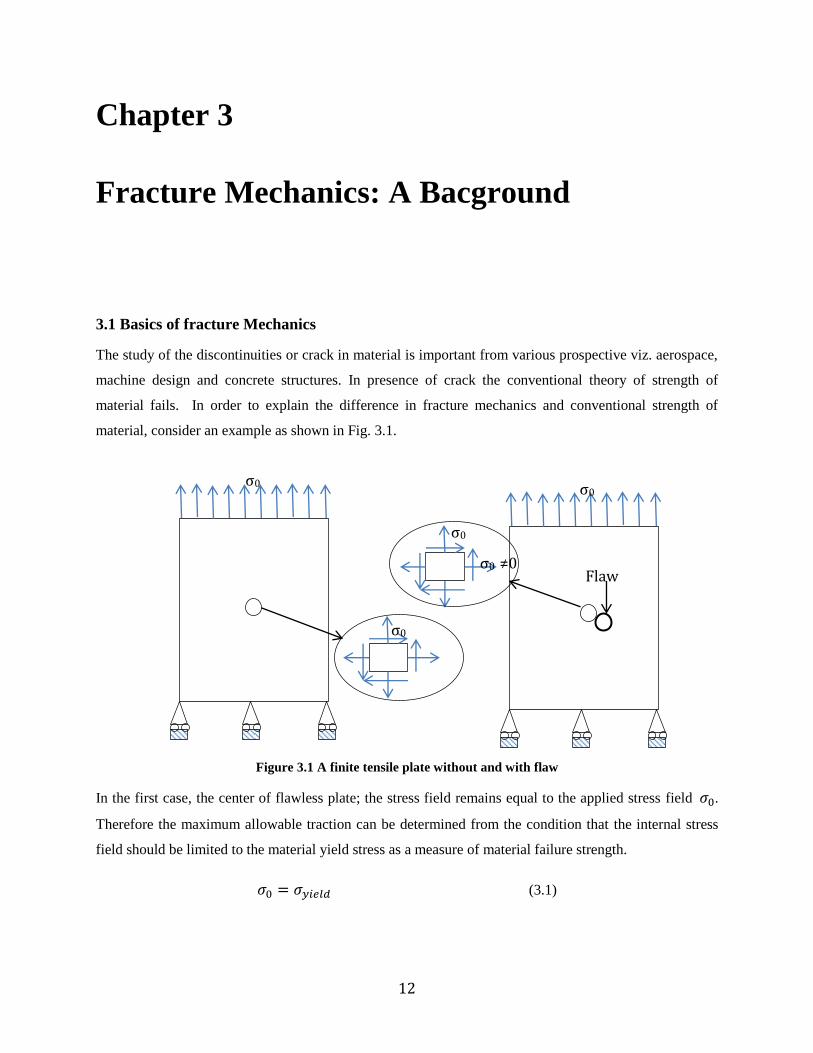
material, consider an example as shown in Fig. 3.1.

Figure 3.1 A finite tensile plate without and with flaw

In the first case, the center of flawless plate; the stress field remains equal to the applied stress field .

Therefore the maximum allowable traction can be determined from the condition that the internal stress

field should be limited to the material yield stress as a measure of material failure strength.

(3.1)

σ0

σ0 ≠0

σ0 σ0

Flaw

σ0

13

In contrast, the elasticity solution for an infinite plate with circular hole or defect predicts the biaxial non-

uniform stress field with a stress concentration factor of 3 at the center of the plate, regardless of the size

of the hole. In the limiting case of line crack, the solution from a degenerated elliptical hole shown in

infinite stress state at a crack tip. No material can withstand such an infinite stress state. Therefore,

instead of comparing the existing stress field with strength criterion, fracture mechanics adopts a local

stress intensity factor or global energy release rate and compare them with their critical values.

3.2. Modes of fracture failure

State of stress field ahead of the crack tip depends on the curvature of the discontinuity. Usually crack has

different curvature. Thus there is a large variation in the stress field near to the crack tip. The curvature of

the crack depends upon the modes of the failure and these modes of failure can be divided into three types

depending on the loading conditions. Various modes of failure have been shown in Fig. 3.2. Mode I is

opening mode and displacement is normal to crack the surface. Mode II is the sliding mode and

displacement is in this mode is in plane of the crack. The relative displacement is normal to the crack

front. Mode III is also same as Mode II which is caused due to sliding. But in this case displacements are

parallel to the crack front, thereby causing tearing.

y

x

z

Mode I

Mode II

Mode III

Figure 3.2 Modes of fracture failure

14

An inclined crack can be simulated as the combination of the all the three modes of failure. It can be

modeled as superposition of two or three modes of failure depending on the loading criterion. Effect of

loading can be analyzed separately for each mode and it can be superimposed under the linear elastic

system.

3.3 Stress Intensity Factor

The strength of any material can be defined as the resistance of the body at the extreme loading

conditions. This resistance is calculated at the critical part of the domain. In case of fracture problem, the

region ahead of the crack tip is very critical. Stress field ahead of crack tip is a function of two variables

i.e. loading and the crack length. In the engineering field, solving a problem with two variables is much

more difficult. It also impacts on the computational cost. Keeping this point in the mind Irwin (1957)

introduced the concept of Stress Intensity Factor (SIF) , as the measure of strength of the singularity.

He illustrated that the entire elastic stress field around the crack tip are distributed similarly and

√ controls the local stress quantity. Stress field ahead of the crack tip can be expressed as

{ ( )

( ) ( )} (3.2a)

Where is the stress field and and are the stress intensity factors for the various modes of

failure. and are the radial coordinate of the material point. is the trigonometric function

defined and coordinate system.

√ (

) (3.2b)

are the constants. In terms of the applied stress, Stress intensity factor can be expressed as

√ (3.3)

√ (3.4)

√ (3.5)

Combining the equation (3.2), (3.3), (3.4) and (3.5), we will get the expression for stress field. Stress field

and displacement field can be written in terms of stress intensity factor (SIFs). These expressions are as

follows:

15

For pure opening Mode I, Stress field is given by

√

(

) (3.6)

√

(

) (3.7)

√

(

) (3.8)

Displacement field is given by,

√

(

)

(3.9)

√

(

)

(3.10)

For the pure mode II, Stress field is given by,

√

(

) (3.11)

√

(

)

(3.12)

√

(

)

(3.13)

16

Displacement field is given by,

√

(

) (3.14)

√

(

) (3.15)

The tearing mode III has only two non-zero stress components and one non-zero displacement

component

√

(3.16)

√

(3.17)

(3.18)

√

(3.19)

Where

{

and are the Poisson’s ratio and bulk modulus respectively.

3.4. Direct Method to determine the fracture parameters

Finite element analysis of the fracture problem can be done using either triangular element (3 or 6-

Noded), or quadrilateral element (4 or 8 Noded). FEM analysis will give the stress and displacement field

over the entire domain at the nodal points. Making use of direct available expression of stress and

displacement fields [eqns (2.6-2.19)], we can estimate the value of and .

Ideally and should be determined by the stress field at point ahead of the crack tip. It is very

difficult to get the stress values ahead of the crack tip. The stress singularities are present at the tip of

discontinuity. These stress singularities give a very high SIF value. It is challenging work to mimic the

exact stress state ahead of the crack tip. In order to find out the SIF value, we can plot the curve between

normalized radius and normalized SIF values for some assumed nodes. This curve will not start from zero

17

radiuses, hence extrapolation and curve fitting is required for the estimating value at the zero radius. This

estimated value can be used as normalized SIF for the given problem.

3.5 Calculation of SIF from J-Integral

J-Integral is defined as

∫ (

)

(3.20)

Where ∫

is the strain energy density and is the traction. The contour starts from one

crack surface and end at the other end of crack surface as shown in Fig. 3.3. This integral can be

evaluated on the path which is slightly away from the crack tip, so that the modeling errors can be

minimized. It allows the freedom to make any choice for the computation of the J-Integral. The Path for

computation of J-Integral is independent of path.

Knowing the J-Integral value, then the evaluation of the stress intensity factor (SIF) is straight forward.

We can use the following expression to calculate the SIFs.

(3.21)

Where {

(3.22)

𝑇𝑖

𝑛𝑖

𝑑𝑠 𝑥

𝑥

Figure 3.3 Path Г around the crack tip with outward normal

Г

18

3.6 J-Integral: Definition

J – Integral is a characterization parameter of the fracture problem. It characterizes the state of affairs in

the region ahead of the crack tip. Energy release density (G) is a special case of the J-Integral. G is limited

to the linear elastic material, whereas J-integral is applicable to all kinds of material behavior i.e. linear,

non-linear, hyper-elastic and many more. J-integral is best suitable parameter to be determined as the

crack tip exhibits the elastic-plastic behavior.

For a plane problem, consider a path around the crack tip which starts from one surface of the crack and

ends at the other surface of the crack. This path is arbitrary in nature. It can be smooth or it may have

some sharp corner but the path should be continuous and should be within the material. J-integral was

first applied to fracture problems for plane problem. J-Integral is defined as

∫ (

)

(3.23)

Where ∫

is the strain energy density and is the traction

For 2 –D case can be expressed in full form as

∫

∫

∫

∫

(3.24)

For symmetric and elastic problem , hence

∫

∫

∫

(3.25)

Traction at the point on the path is expressed through well-known Cauchy’s relation .

Thus by knowing the stress field and direction of the normal at the point on the path , we can determine

the . Finally we can come up with the value of the J-Integral.

3.6.1 Properties of the J-Integral

J-integral has the following properties:

1. J-Integral is path independent, i.e. The path can be any arbitrary path within the domain.

2. For linear elastic materials, the J-integral is same as the energy release rate

19

3. J-Integral can be related to the crack tip opening displacement by the simple relation of the

form . Where is dimensionless number, is far field, is opening

displacement.

4. J-Integral can be easily determined by the experiments.

3.6.2 Determining the fracture parameter form FEM solution

In general the displacement and stress fields are known as the solution from FEM or any other simulation

technique. These displacement fields and stress field can be used to determine the SIF of the problem. SIF

can be calculated from the equation given below

√

( )

(3.26a)

√

√ ( )

(3.26b)

Where ( ) and

( ) are the functions defined in terms of and [eqn (3.2b)] . is stress field,

is displacement field.

For Mode-I equation 3.26 can be written as

√

(

)(

) (3.27a)

( ) √

√ (

)(

) (3.27b)

Theoretically the crack tip has stress singularity, so to minimize the errors an arbitrary path has been

taken for computation of the fracture parameters. SIF has been calculated at all the gauss point along the

selected path. This SIF evaluation can be made either from displacement field or from stress field. They

are plotted on a graph taking radial distance in x-axis. Both the axes are normalized. Actual SIF value has

to be calculated at the crack tip at the radius but this plotted graph does not give the same. This

graph has to be fitted to get the value at zero radius. Curve fitting is done with higher order polynomial to

obtain the value at radius zero. This curve fitted value is considered as the SIF. J-Integral is calculated

from the equation 3.21.

20

Chapter 4

Generalized finite element Method

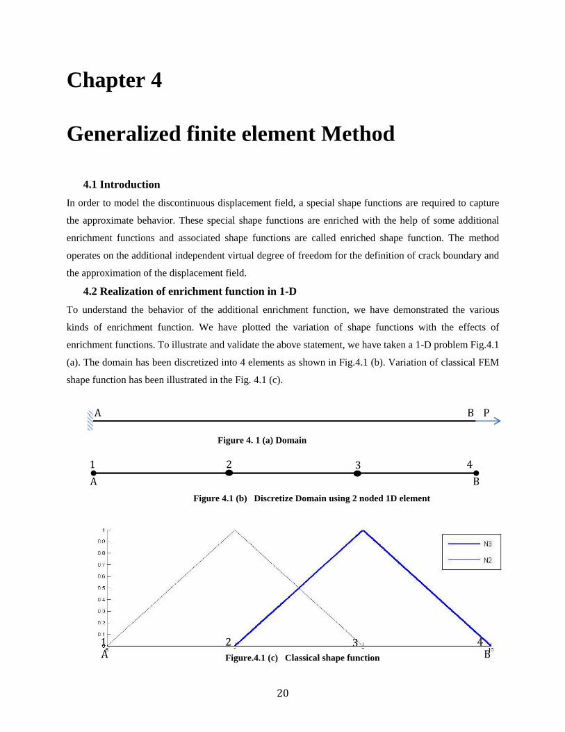
4.1 Introduction

In order to model the discontinuous displacement field, a special shape functions are required to capture

the approximate behavior. These special shape functions are enriched with the help of some additional

enrichment functions and associated shape functions are called enriched shape function. The method

operates on the additional independent virtual degree of freedom for the definition of crack boundary and

the approximation of the displacement field.

4.2 Realization of enrichment function in 1-D

To understand the behavior of the additional enrichment function, we have demonstrated the various

kinds of enrichment function. We have plotted the variation of shape functions with the effects of

enrichment functions. To illustrate and validate the above statement, we have taken a 1-D problem Fig.4.1

(a). The domain has been discretized into 4 elements as shown in Fig.4.1 (b). Variation of classical FEM

shape function has been illustrated in the Fig. 4.1 (c).

Figure 4. 1 (a) Domain

Figure 4.1 (b) Discretize Domain using 2 noded 1D element

Figure.4.1 (c) Classical shape function

P B A

1 2 3 4

1 2 3 4

B A

B A

21

If the same domain has a discontinuity as shown in Fig.4. 2 (a) as well as the discretization is also same as

for the continuous domain, then Node 2, 3 are required to be enriched, whereas Node 1 & 4 are not

influenced by the discontinuity.

There have been a number of possibilities of enrichment function, which can be used to simulate the

strong discontinuity in the domain. Few of them are illustrated here.

Enrichment function in 1-D

4.2.1 Partition of Unity Method: A simple Model

In the development stage of XFEM, many researchers had used the concept of partition of unity

approach to find out the enriched shape functions. Enriched shape function has been defined as

the following

{

(4.1)

Fig. 4.3 shows the jump in the basis functions which are capable of capturing the discontinuity in

the domain. This kind of jump function provides the same strain field in the both sides of the

discontinuity. This is in contrast to independent physical response of segment anticipated in

Figure.4.2 (a) Discontinuous Domain

Figure.4.2 (b) Discretize Domain (Red Point –Enriched Node)

1 2 3 4

Figure 4.3 Jumps in the shape function using the Partition of Unity Concept

P

B A x=a

Line of discontinuity

B A

2 3

22

cracked domain. For this jump methodology, a lesser number of additional Dofs are required than

other methods. Thus it cannot be a better method to be used for simulating the cracked domain.

4.2.2 The Heaviside function

Heaviside function has been defined in various manners over a decade. Definition of Heaviside

function has been modified depending on the problem statement. Classical or first type of

Heaviside function has been defined on the basis of step function. Mathematically it can be

written as an equation (3.2). A variation of it has been shown in Fig. 4.4 (a).

( ) {

(4.2)

The effect of the step Heaviside function has been shown in Fig. 4.4 (b). Now the strain fields are

independent for the both sides of the discontinuity. Here shifting is defined as the difference

between the classical and enriched shape function and it has been shown in Fig.4.4 (c). If we see

the variation of the shape function, it has value equal to the zero on the left side of discontinuity.

This observation shows that these types of enrichment functions are not capable of capturing the

exact behavior in the both sides of cracked domain.

Figure.4.4 (a) Step Heaviside Function

Figure 4.4 (b) Effect of Step Heaviside Function on 1-D FEM Shape function

2 3

23

4.2.3 Modified Heaviside function

To increase the capability of Heaviside function, it has been modified with the help of the sign

function. It is also called as signed Heaviside function. It can be expressed as follows

( ) {

(4.3)

The variation of the modified Heaviside function is shown in Fig.4.5 (a). It has value equal to 1

and -1, which helps in capturing the behavior in the both sides of the crack. It also ensures the

independency of the strain field in the both sides of the discontinuity. Enriched shape function

variation has been plotted in the Fig.4.5 (b) and its shifting has been illustrated in Fig. 4.5 (c).

Figure 4.4 (c) Shifting of 1-D FEM shape function

Figure 4.5 (a) Sign Heaviside Function

2 3

24

4.3 Realization of enrichment function in 2-D

The main objective of enrichment function is to reproduce the singularity around the crack tip. It can be

achieved by using terms containing trigonometric functions. In order to model the discontinuous

displacement field, a special kind of shape functions is required to capture the approximate behavior. The

method operates on the additional independent virtual degree of freedom for the definition of crack

boundary and the approximation of the displacement field.

Figure 4.5 (b) Effect of Sign Heaviside Function on 1-D FEM shape function

Figure 4.5 (c) Shifting of 1-D FEM shape function

2 3

2 3

25

Figure 4.6 (a) Patch of 4-element (b) Classical shape function or hat function

Various kinds of enrichment function for 2 –D are listed below

Modified Heaviside function

Crack tip enrichment function

Level set enrichment function

The variation and its effect on the approximation function have been discussed in the following section.

4.3.1 Modified Heaviside function

Heaviside function is discontinuous along the crack path which insures the presence of discontinuity in

the approximation. These discontinuities can be easily modeled using these kinds of enrichment function.

A variation of the Heaviside function is shown in the Fig 4.7. Mathematically it can be written as follows:

( ) {

(4.4)

(1) (2)

(3) (4)

(a) (b)

26

Figure 4.7 (a) Variation of Modified Heaviside Enrichment function in 2-D (b) Cracked Domain

Figure 4.8 Variation of enriched shape function (N1-N4) with implementation of Modified Heaviside

Enrichment

(a)

(b) Bilinear element

1 2

4 3

Line of discontinuity

y

x

27

If an element has a crack as shown in the Fig.4.7 (b), then the variation of Heaviside function is as shown

in Fig. 4.7 (a). When this enrichment function is multiplied with the classical shape function or hat

function, then enriched shape functions are obtained. These enriched shape functions are depicted in the

Fig. 4.8.

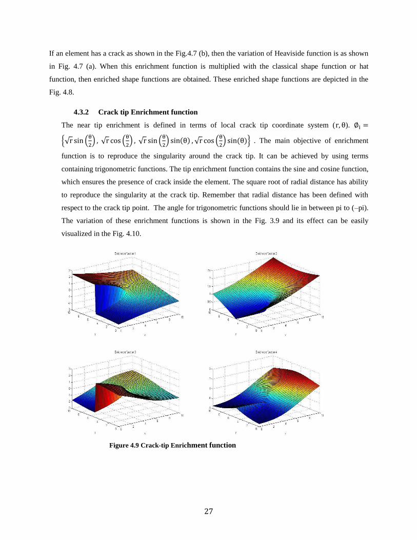
4.3.2 Crack tip Enrichment function

The near tip enrichment is defined in terms of local crack tip coordinate system ( ).

{√ (

) √ (

) √ (

) ( ) √ (

) ( )} . The main objective of enrichment

function is to reproduce the singularity around the crack tip. It can be achieved by using terms

containing trigonometric functions. The tip enrichment function contains the sine and cosine function,

which ensures the presence of crack inside the element. The square root of radial distance has ability

to reproduce the singularity at the crack tip. Remember that radial distance has been defined with

respect to the crack tip point. The angle for trigonometric functions should lie in between pi to (–pi).

The variation of these enrichment functions is shown in the Fig. 3.9 and its effect can be easily

visualized in the Fig. 4.10.

Figure 4.9 Crack-tip Enrichment function

28

4.3.3 Enrichment function by Level set

The level set function is defined as a function of location of crack propagation. And the minimum

distance has been plotted a surface plot in Fig 4.11. This has been used as enrichment function. These

enrichment functions are most suitable for dislocation and hole modeling problems. The effects of

these enrichment functions can be seen in Fig 4.14. Mathematically level set can be expressed as

follows.

( ) { ( )

( )

(4.5)

( ) ‖ ‖ (4.6)

Figure 4.10 Basis function with Crack-tip Enrichment function

29

Figure 4.11 Level set in Y-direction

Figure 4.12 Variation of the level set function in X-direction

30

Figure 4.13 Variation of Level set function in case of inclusion or circular discontinuity

Fig. 3.11 illustrates the variation of a minimum distance of the point from the cracked portion.

Mathematically it is the perpendicular distance between the point and the crack. Fig 3.12 shows the

variation in the Y-direction. It is the minimum distance between the crack tip and any arbitrary point in

the domain. In case of inclusion and circular discontinuities, level set is defined on the basis of radial

distance of the material point. It depends on the given radius of inclusion. The variation of such kind of

level set is presented in the Fig. 3.13. These level set functions are very good in capturing the dynamic

crack. Level set function for arbitrary crack has been plotted in the Fig. 3.14. Enriched shape function is

also plotted in the same figure.

31

Figure 4.14 Top: hat function or classical shape function, Middle: Level set to arbitrary crack,

Bottom: Enriched shape function with the implementation of middle function. Enriched shape

function is obtained by the multiplication of the hat function and level set

4.4 Conclusion

Enrichment functions are the key function in GFEM context. These enrichment functions are

capable to mimic the exact behavior ahead of the crack tip. Level set based enrichment functions

are capable to entertain the material behavior in the simulation of composite materials. 3-D crack

can be captured with the help of the level set based enrichment functions. The various

enrichment functions have been studied in this chapter. Their application and their potential have

been described through examples. 1-D and 2-D examples have been illustrated here.

32

Chapter 5

Blending Element

5.1 Introduction

Application of the enrichment near the crack tip analysis leads to solution incompatibility and interior

discontinuities, if it is not employed in the entire domain. Since neighboring domains are using the different basis

function and approximation, it can attribute the incompatibility of the solution. There is a transition from classical

FEM approximation to the enriched FEM approximation. As a result the different value may be obtained for the

same node. Occurrence of the different values shows the interior discontinuities.

Main Issue related transition of approximation in GFEM

1. Convergence of the solution is not guarantied.

2. Enrichment does not follow the partition of unity method properties. Hence the order of convergence and

error may get affected

Seeing these drawbacks in GFEM/X-FEM, It became an essential requirement to rewrite the approximation for

Blending elements. It is suggested to write down the approximation in the following form

( ) ∑ ( )

( )∑∑ ( ) ( )

Where ( ) is called Ramp function or Blending functions, ( ) are classical shape function, enriched shape

functions, are the additional Dofs . All other terms have usual meaning. This function should have some

essential properties.

5.2 Problem Statement

1. A blending function, which can be helpful in a smooth transition between enriched, and unenriched

domain (Classical domain) is required.

33

2. Enrichment function, which should not produce parasite, terms in the approximation so that the ability to

reproduce the stress/strain condition can be retained.

5.3 Literature Survey

Blending element was first introduced by Sukumar [52] in XFEM with the level set method. In this work they had

used ramp function as blending function. Blending element is an element whose some of the nodes are enriched

and some of the nodes are classical node. A broad framework has been developed by Chessla et.al [28, 29, 32] to

sort out the problems associated with parasitic terms in the approximation. To this end enrichment of the strain

field is done instead of directly enriching the approximation.

Many researchers have used so many techniques to sort out the problems related to blending elements. Chessla

et.al [32] had used assumed strain method to eliminate the parasite terms in the approximation. The larger

approximation space of higher order spectral element has been also shown to improve the accuracy in the blending

element. Gracie [53] has used discontinuous Galerkin [54] method to overcome the spurious behavior of blending

element. In this method domain is divided in two parts as enriched and unenriched patches, which are

independently discretized. Continuity in the patches is enforced in the weak sense by internal penalty method.

Intrinsic XFEM and discontinuous enrichment methods are two methods to not have blending elements. Fries [55]

have proposed a method based on the weighting of enrichment that vanishes at the edge of enriched subdomain.

5.4 Classification of the elements

Due to different approximation function, finite elements used in GFEM can be classified into three categories

(a) Classical Element

(b) Enriched Element

(c) Blending Enrichment or Partial Enriched Element

First two categories are fully governed by the classical and enriched approximation respectively, whereas the

blending element is governed by the combination of both approximations. Classification of the element is shown

in the Fig. 5.1. In the Fig. 5.1 green color shows the element with discontinuity, which has enriched

approximation. The neighboring elements shown in red color are partially enriched element. They are governed by

the combination of approximation of classical as well as enriched approximation. Remaining blue color elements

are the classical elements, which are governed by the classical approximation.

34

Figure 5.1 Classification of Element a) Green- Enriched (b) Red- Blending (c) Blue- Classical Element

5.5 Characteristics of Blending or Ramp function

Linear and spline function are frequently used as ramp function. These functions should have the following

characteristics in them.

1. Define the appropriate ramp function to satisfy the C0 and C

1 continuity between the enrichment and classical

finite element approximation.

2. Linear and spline functions are usually preferred.

3. The size of transition zone should be selected.

4. Compute the necessary term associated with the transition domain.

5. The number of enriched and classical nodes in the transitional finite element may suddenly change in nearby

elements. Special precautions are required to avoid potential mistakes in defining the correct numbers for

different summation.

5.6 Properties of Blending Function:

1. Co-ordinate independent: Blending functions should be co-ordinate independent. It emphasizes that

the function should not change in as there is any change in coordinate system. In order to show for co-

ordinate independency blending function should follow the Partition of Unity (POU). The property of

co-ordinate independence is also called as affine invariance. Mathematically id can be written as

∑

2. Convex hull properties: Convex hull is set of point in in a real vector space which contains the

optimal and minimal points. This property exists in the functions which are co-ordinate independent.

In this case the blending function is non-zeros. Mathematically it can be expressed as follows:

Blending Element

Classical Element

Enriched Element

35

∑ ( ) ( )

3. Symmetric functions: if the function value does not change with the change of sequence of data

points or domain, then these functions are called as symmetric function. For a function symmetricity

can be assured if and only if

∑ ( ) ∑ ( )

This hold true if ( ) ( )

4. Variation Diminishing Properties: B-Spline and Bezier always obey these properties. It says that if a

given straight line intersects the curve in c number of points and the control polygon in numbers of

point then it will hold true

Where is any positive integer

5. Linear Independence: A set of blending functions is linearly independent. Mathematically it can be

written as follows

∑

Where are random constants. If blending functions are not linear independent, then one

function can be written as a combination of other functions. This will affect the order of

approximation.

6. End Point interpolation: Blending functions are interpolatory in nature. But they interpolate the

value at the end points. Due to this interpolation properties blending function are much more useful in

X-FEM/G-FEM. It interpolates the value of classical node as well as at enriched node. This provides a

smooth transfer from classical to enriched approximation.

5.7 Examples of Blending Function:

a. 1st order Blending Function: It has value as zero or one. It's defined as the following

( ) {

b. 2nd

order Blending Function: it’s obtained from the 1st order blending function. After integrating the

1st order blending function, 2

nd order is obtained. It is defined as the following

( ) ∫ ( )

36

( ) {

c. 3rd

order Blending Function: 3rd

order is obtained from the integration of 2nd

order blending

function. It has been defined as the follows

( ) ∫ ( )

( ) {

(

Figure 5.2 (a) 1D blending element (b) bilinear blending element, Variation of Blending or Ramp function in (c) 1D (d )2D

1 2

3 4

(b)

1 2

(a)

(c) (d)

r

𝑅(𝑥)

1

1

2

2

3

4

37

5.8 Blending Function used in Thesis

Our approach is based on local enrichment function, which results out as transition of approximation between

the two neighboring elements. Thus the blending element became an important issue. As we have seen earlier

that it can be solved using the blending function. There are various kinds of Blending functions. We have used

first order Blending function as shown in Fig.5.2.

Blending function has variation from 0 to 1. It has value equal to one of the enriched node and has a value

equal to zero at all other nodes. Fig. 5.2 (a) and (b) shows the 1-D and 2-D domain respectively. Lets assume

that node 1 is enriched incase of 1-D and node 4 in case of 2-D problem (Fig.5.2 (a) & (b). All other nodes are

classical nodes. For one dimensional and 2-dimensional problem, variations are shown in the Fig.5.2 (c) and

(d) respectively.

The strategy follows the following steps:

(a) Begins with standard partition of unity approximation

(b) Multiply the origin enrichment function by monotonically decreasing weight function with compact

support.

(c) Constrained all the enriched degree of freedom to be equal. Weight function is used in such a manner

to avoid inter-element discontinuity.

5.9 Conclusion

In this chapter various blending functions has been studied. This chapter emphasis on the need of the

blending functions. Classification and properties of the blending functions are described in detail. Variation

of the blending function has been demonstrated though an example. Implementation strategy has been

discussed.

.

38

Chapter 6

Galerkin Formulation and GFEM

Implementation

6.1 Introduction

This chapter is concerned with Galerkin formulation of equilibrium governing equation. Classical

formulation is limited to classical degree of freedom but in case of GFEM some additional degree

of freedoms are introduced. These additional degrees of freedoms are consolidated to the

discontinuous element. The formulation of these discontinuous elements allows the simulation of

the crack propagation without remeshing. A detail of the numerical implementation has been

given in this chapter.

6.1.1 Governing Equation

Consider a body in the state of equilibrium with the boundary conditions in the form of tractions and

displacement conditions as shown in the Fig.6.1

Figure 6.1 Body in static equilibrium

The strong form of the equilibrium equation can be written as

(6.1)

With the Boundary conditions

39

{

(6.2)

Where and are the traction, displacement, and cracked boundaries respectively. is the

stress 1st order tensor. is the body force. is the applied traction force on the traction boundary.

From the principle of virtual work, the variational formulation of the boundary value problem can be

defined as

(6.3)

Integral form of the equation can be written as

∫ ∫ ∫ (6.4)

5.1.2 GFEM discretization

The discretization of the equation (6.4) using the GFEM approximation (equation (6.1)) results

into the system of linear equilibrium equations:

(6.5)

Where is the stiffness matrix. is the vector of nodal freedom (enriched and classical

combined), is the vector of the external forces. The global matrix and vectors are calculated by

the assembling the element stiffness matrix and element vectors. and for each element are

defined as

[

] (6.6)

{

} (6.7)

And is the vector of nodal parameters

{ } (6.8)

With

40

∫ (6.9)

∫

∫

(6.10

∫ ∫

(6.11)

∫

∫

(6.12)

In the equation (6.9) , the is the shape function derivative.

[

] (6.13)

[

] (6.14)

[

] (6.15)

[

] (6.16)

Where

The crack tip enrichment functions have been defined in the terms of the local crack tip co-

ordinate system as shown in the Fig.6.2. Mathematically it can be rewritten as

{√

√

√

√

} (6.17)

Derivative of with respect to the crack tip polar coordinate becomes

√

(6.18)

√

(6.19)

√

(6.20)

√

(6.21)

41

√

(6.22)

√ (

) (6.23)

√

(6.24)

√ (

) (6.25)

Where and are defined in terms of the global coordinate systems

√( ) ( )

(6.26)

(

) (6.27)

The derivative of the and with respect to the global coordinate system can be written as

√( ) ( )

(6.29)

√( ) ( )

(6.30)

(

)

( ) (6.31)

(

)

( ) (6.32)

Finally the derivatives of the crack tip enrichment function with respect to the global coordinate

system can be written as

(6.33)

(6.34)

42

6.2 Numerical Integration

The Gauss quadrature rule is widely used in finite element analysis for the numerical integration of

stiffness matrix and other integral evaluation over a given domain. For the polygonal integrand the

gauss quadrature is proved to be more accurate. In case of non-polygonal integrand it may result with

some errors. Thus it may result some substantial accuracy reduction in output. For better results of

numerical integration of more and more Gauss points are required. Less number of Gauss point may

cause the various unavoidable errors.

Gauss Integration scheme is only applicable to the continuous function and over a continuous domain.

In the presence of discontinuity, this numerical scheme get fails. This is further complicated as the

crack path turns to be substantially curved. As a result, an efficient approach is required to define the

necessary points needed for the integration points within the enriched element. This scheme has to be

consistent with the geometry of the crack as well the order of the enrichment functions.

Because ordinary gauss rule do not calculate the integration of enrichment element. Dolbow [56] has

proposed two methods to overcome the numerical integration difficulty. He talked about the

portioning of the enriched element. He proposed that an enriched element can be sub-divided into the

sub-triangles or the in the sub-quds.

6.2.1 Partitioning of element

An enriched element can be sub- divided into sub triangles or into the sub-quads. These two

approaches are available for the improvement of the numerical integration. These two methodologies

are described as below.

Ω

Гc

r θ

x

y

Figure 6.2 Polar Coordinate near the crack tip

43

Sub-quads

In this method

The element domain is uniformly partitioned into a regular subgrid of quadrature

elements (sub-quads)

Each sub-quad is assigned a predefined set of gauss quadrature points and

corresponding weight function.

The integrand and weight functions are computed at each gauss point.

The final solution of the integral is obtained from the summation over all gauss points

within the elements.

A node is enriched only if there exists at least one Gauss point both side of the crack.

Sub-Triangles

This is an alternative to sub-quad approach by construction of local mesh of the triangular

quadrature elements between the crack and element boundaries.

Determine whether the crack crosses the element

If the area between the crack and the corner node is very small compare to the element

area, neglect the presence of crack and avoid the sub-triangulation

Use a simple triangulation technique by adding a limited predefined numbers of the

points inside an element and on its boundaries and connecting them t form consistent

well shaped triangles

A local Delaunay triangulation scheme may always be used as an automatic approach

for the creation of quadrature sub-triangles.

Each sub-triangle is assigned a predefined set of gauss points and corresponding weight

function.

The integrand and the weight function are computed at the every Gauss point.

The final solution of the integral is obtained from the summation over all the gauss

point within the element.

Figure 6.3 Partitioning of the element

44

6.3 Selection of Enriched Node

In the proposed methodology of GFEM, the approximation is enriched at the local level and it

confined to the discontinuous domain. It means that selection of node to be enriched is an issue. There

are various different ways to select a node for the enrichment process. Fig.6.4 shows the simple

procedure to select the node for enrichment. At the each stage of propagation of the crack, nodes of

that element will get enriched. If a crack touches the boundary of one element but does not go inside

that element, then nodes of that element will not be enriched as shown in the Fig.6.4 (c).

Figure 6.4 Enriched node at different stage of crack propagation (Black dot shows the enriched node)

The technique adds some additional degree of freedoms per node. The numbers of additional degree

of freedoms depends on the choice of enrichment function (i.e. Heaviside function, crack-tip

enrichment function or level set). Selection of the enrichment function is discussed in the next section.

(a) (b)

(d) (c)

45

6.3.1 Criterion for Node enrichment

1. First criterion is based on the area enclosed by the discontinuity. Fig. 6.5 (a) shows the area

distribution with discontinuity. If the value of area ratio

is less than 0.01% then that

node may not be enriched. If area ratio is more than 10% then the enrichment of node is

compulsory.

Figure 6.5 (a) description of area (b) existence of gauss point

2. Second criterion is based on the location of gauss point within the elements. According to this

criterion if the gauss point is enclosed by the crack domain, then corresponding Node has to

be enriched. If it’s not enclosed, we have freedom for not enriching that node. As shown in

the Fig.6.5 (b) gauss point corresponding to node 1 is outside the cracked domain, hence it

gives freedom for enriching the node while Gauss point corresponding to node 2 is inside the

domain. It’s compulsory to enrich the node 2.

6.4 Assembly of the Global stiffness matrix

In classical FEM we assemble the nodal displacement vector based on the node numbers. In case of 2-

dimensional problem the rth node will contribute for the (2r-1) and (2r) degree of freedom in the

global matrix.

Same node will be responsible for (2r-1) & (2r) rows and column in the global stiffness matrix. It’s

always easy to implement it. In the case of GFEM, there are some additional degrees of freedoms.

Now the challenge is that how to assemble these degrees of freedoms in the global stiffness matrix.

𝐴

𝐴

1

2

(a) (b)

46

To assemble the additional Dofs, we have used the concept of the phantom nodes. These are virtual

nodes and have no physical understanding. These are some random nodes which have numbered just

after the number of real nodes. Number of phantom nodes depends on the type of enrichment function

as well as the number of enrichment functions.

The 1-Phantom Node is required for Heaviside-Enriched Element

4- Phantom Node is required for crack tip Enriched Element

6.5.1 Example of Phantom node implementation

Suppose a set of node N= [1, 2, 3, 4, 5, 6, 7] is given, In which the node number [3, 5,7] are Heaviside

enriched and node [6] is enriched with the help of crack tip enrichment functions. A matrix of size

1*7 (ADN= [0, 0, 0, 0, 0, 0, 0]) is created. This ADN matrix is then updated according to the

enrichment function and number of phantom or additional nodes. In this case after assigning the

global number to the phantom doffs the ADN matrix will become ADN= [0, 0, 8, 0, 9, 10, 14]. Node

number 3 and 5 are Heaviside enriched hence a next number is assigned to these places. Node number

6 is enriched by crack tip enrichment function; hence it required four phantom numbers. Due to

presence of crack tip enrichment at node 6 next enriched nodes (i.e.7) got the global number as 14

(i.e. 9+4+1=14). Now the displacement vector will become as follows

Where is the nodal displacement at node, is the additional dofs at the th node due to Heaviside

enrichment, is the additional dofs at the th node due to crack-tip enrichment

6.6 Conclusion

Detailed formulation of governing equation has been derived in this chapter. This

formulation is done for enriched approximation. Numerical implementation issues are

discussed in this chapter. Numerical integration and assembly of the global stiffness matrix

has been illustrated with the help of an example. The concept of phantom node has been

described with example.

47

Chapter 7

Numerical Example: Stress Analysis and SIF

Study

7.1 Problem definition

In order to check and validate the robustness and efficiency of the proposed two scales GFEM, standard

problems of the fracture mechanics has been solved as numerical examples. We have considered a 2-D

plate with dimension units, unit. Young’s modulus has been taken as units,

Poission’s ratio is . Edge crack and inclined crack fracture problems have been illustrated the

efficiency of the Multiscale GFEM. Plane stress condition has been considered with thickness of 1 unit.

A 4-noded bilinear element has been used for the discretization of the domain. The approximation of

bilinear element is enriched with the help of the Heaviside function and crack tip enrichment function. 4

crack tip enrichment function has been used. Due the presence of the crack tip enrichment function and

Heaviside function, the size of the element stiffness matrix increases from the classical 8*8 to 48*48.

There is an increment of the 40 rows and column in each enriched element. Similar effects are in In case

of blending element, all the nodes are not enriched. Classical nodes add numerical instability in global

stiffness matrix by addition of zero rows and column. This instability has been improved by the

elimination method. Rows and columns corresponding to the additional dofs of classical nodes within the

blending element are eliminated from the global stiffness matrix.

7.2 Modeling 2-D Edge Crack Problem

A 2-dimensional plate with the dimension units, units has been considered for an edge

crack problem. Crack length has been taken as units. Domain dimensions and the Boundary

conditions are shown in the Fig.7.1 (a). Edge crack is located at the mid height of the plate. Top edge of

the plate has been given the displacement of units. Bottom edge is constrained in the Y-direction.

The bottom node on the right side is also constrained in the X-direction to prevent the rigid body motion

in the X-direction.

48

Figure 7.1 (a) Edge Crack Problem (b) Inclined Crack Problem

7.2.1 Elastic Analysis

For an elastic analysis of the material properties has been taken as Young’s modulus units,

and Poission’s ratio . The problem has been solved using 4-noded quad element

approximation. Fig.7.2 shows the contour plot of the stress in Y-direction and X-direction respectively.

Figure 7.2 Stress Plot for Elastic Analysis of an Edge Crack Problem

a L

B

a L

B

(a) (b)

𝜎𝑦𝑦 Plot 𝜎𝑥𝑥 Plot 𝜎𝑥𝑦 Plot

49

(Note: Normalized SIF=

√ and Number of Dofs in one direction is =√ )

Figure 7.3 Mesh Independency Study

In order to say that proposed method is mesh independent, we have done the Stress Intensity Factor

(SIFs) evaluation with different meshes. Fig. 7.3 shows that there is an increment in normalized SIF with

the increment of the number of degrees of freedoms in the domain. But this increment is not so large. It

becomes a flat curve after a certain number of degrees of freedoms. Observation indicates that proposed

method took a very small number of the elements as compare to the classical FEM analysis of the fracture

problems. It can be concluded that the developed method is mesh independent. It’s not a mesh free

method but it’s a mesh independent methodology.

7.2.2 Hyper-elastic Analysis

Mooney-Rivlin material model has been used for simulating the edge crack problem with the help of

GFEM. Mooney-Rivlin is a hyper elastic material model in which the strain energy is defined as the linear

combination of the two invariant of the left Cauchy’s Green deformation tensor. This method was

proposed by Melvin Mooney in 1940 and expressed as a linear combination of invariant in 1948 by Ronal

Rivlin.

50

Constitutive relation to Hyperelastic Analysis:

A quadratic isotropic function of the Green strain tensor

( ) can be used to define the constitutive

relation. From the St. Venant material principle the stored energy can be written as

( ) ( )

Where and are Lame’s parameters. We can simplify this expression to

( )

The strain energy density function for Mooney Rivlin can be written as

( ) ( )

Where and are first and second invariant of the unimodular component of the left Cauchy-Green

deformation tensor. These invariants are defined in term of stress invariant and .

⁄

⁄

Where the constant for incompressible material

Most generalized forms of the strain energy density with the effect of compressible material can be

rewritten as

( ) ( ) ( )

The hydrostatic pressure can be correlated with energy density function as follows

( )

The hyperelastic analysis is based on the incremental stress and very large deformation. Incremental

stress can be written as

Where and are material response tensor of 4th order and 2

nd order respectively, is Piola-

Kirchoff stress. These tensors can be written as

(

)

⁄

The explicit expression of are as below

51

(

)

(

) (

)

(

)(

)

( )

(

)

(

)

(

)

Where is the th component of the

The same problem of elasticity analysis has been usedinr the hyper-elastic analysis of the edge crack

problem. The coefficient of the strain energy function has been taken as

units, . Where is the bulk modulus. The stress plots of hyper-elastic analysis are shown

in the Fig. 7.4

Figure 7.4 Stress Plot for Hyper-elastic Analysis of Edge Crack Problem

52

7.3 Modeling 2-D Inclined Crack Problem

A 2-dimensional plate with the dimension units, units has been considered for an edge

crack problem. Crack length has been taken as units. Domain dimensions and the Boundary

conditions are shown in the Fig.7.1 (b). Crack is located at the mid of the plate. Top edge of the plate has

been given the displacement of units. Bottom edge is constrained in the Y-direction. The bottom

node on the right side is also constrained in the X-direction to prevent the rigid body motion in the X-

direction.

7.3.1 Elastic Analysis

For an elastic analysis of the material properties has been taken as Young’s modulus units,

and Poission’s ratio . The problem has been solved using 4-noded quad element

approximation. Fig. 7.5 shows the contour plot of the stress in X-direction, XY-direction and Y-direction

respectively.

Figure 7.5 Stress Plot for Elastic Analysis of an Inclined Crack Problem

53

7.4 Conclusion

In the present chapter, numerical examples were illustrated. Capability and the potential of the

GFEM have been illustrated with edge crack and inclined crack problem. Observation of the

results indicates to optimal and efficient simulation tool. It can be concluded that the developed

tool requires a very coarse mesh to capture the complex geometries. Adaptive remeshing is also

not mandatory. It also infers that discrete cracks are not required for modeling static crack. Mesh

independency has been studied through the SIF study with respect to the various mesh sizes.

54

Chapter 8

Sensitivity Analysis

8.1 Introduction

Sensitivity analysis of a solution is the measurement of the uncertainty in the output. It is based on

variational formulation of the continuum mechanics. Structural optimization and sensitivity analysis has

become most popular research field over a decade. Main objective of these kinds of studies is to get most

economical optimized and efficient design. It has wide and enormous application in automobile industry,

aerospace industry, civil structures and many more. It became reliable also due to presence of better

simulation tools. Most of these simulation tools are in-built with the finite element analysis and with

different post processing tools.

8.2 Literature Survey

Bugeda et al. [42] had introduced the methodology for shape sensitivity analysis and they talked about

the shape optimization. Their methodology was based on adaptive mesh refinement. They had validated

their methodology with the help of B-spline functions defined at the boundaries. They have studied the

optimal shape design by controlling the errors and minimizing the same. An error has been controlled by

the means of finite element or boundary element motion and converting the shape derivatives into

differentiations of algebraic equations [43].

Another approach for sensitivity analysis is based on a variational formulation of the continuum

mechanics [44, 45]. In this approach shape sensitivity is simulated with the help of the velocity field. This

velocity field is responsible for the shape change of the body which applies to initial domain. Taroco [46]

had given mathematical formulation of the shape sensitivity analysis in linear elastic fracture problems.

He had established the relation between the domain and boundary expressions for the first and higher

order derivatives of the potential energy stored in elastic body with respect to the shape change.

Chen et. al [47] has illustrated the shape sensitivity analysis of the elastic body with mode-I fracture

problem. B. N. Rao [48] has considered the functionally graded material to demonstrate the capability of

the variational formulation of the sensitivity analysis. He had done the sensitivity analysis for all the

55

modes of fracture failure. Very recently, Edke et. al [49] has implemented the same formulation for the

extended FEM with the level set function as the enrichment function.

8.3 Velocity field

Consider a 3 –dimensional body with domain Ω and boundary Г and body material point have position

vector . Assume that at time T=τ body will have domain and boundary as shown in Fig.8.1.

Figure 8.1 Variation of the domain

Movement from one place to another place can be expressed as

(8.1)

Where are position vectors at different time.

If is the transformation mapping, and is the scalar time with the parameters of shape change

( ) (8.2)

( ) (8.3)

( ) (8.4)

A velocity field can be defined as

( ) ( ) ( ( )) ( ( )) (8.5)

Using Taylor’s expansion and ignoring the higher order terms the transformation mapping can be

approximated by

( ) ( ) ( )

( ) ( ) (8.6)

x

xτ

τV(x)

Ω

Ωτ

Г Гτ

56

There are lots of different methods to define the velocity field [50]. For an edge crack problem we have

considered the velocity variation as shown in the Fig.8.2.

Consider a plate with a horizontal crack with the dimension of L*B. Though we had symmetry but we

had modeled full plate as shown in Fig. 8.4. A PQRS domain has been considered as the domain for the

calculation of J-integral and its sensitivity. The size of this domain is ((2*l1)*(2*b1)), which enclosed the

crack tip inside it as shown in the Fig. 8.2.

The velocity field used in this study has been defined as

( ) { ( ) ( )

{ ( ) ( )

(8.7)

Where

( )

{

| |

(8.8)

( ) {

| |

(8.9)

L

B

2*l1

2*b1

S

P

Q

R

V1=0 V1=0

V1=0

V1=0

x1

x2

V1(x)

Figure 8.2 Schematic diagram of velocity field in the domain

57

7.4 Sensitivity Analysis

The variational form of the governing equation can be written as [51]

( ) ( ) (8.10)

Where and are actual displacement and virtual displacement of the structures and

( ) ∫ ( ) ( ) (8.11)

( ) ∫ ∫

(8.12)

7.4.1 Material derivative

For a given point , material derivative a is expressed as [51]

[ ( ( )) ( )

] (8.13)

If the continuous, then it can be extended in the neighborhood of .

( ) ( ) ( ) (8.14)

Where [ ( ) ( )

]

Material derivative has commutative properties i.e (

)

( )

7.4.2. Variational formulation

Lets assume a domain functional defined over the domain . In the integral form it can be expressed

as

∫ ( ) (8.15)

58

Where is regular function over the domain and domain is regular. For assumed functional

material derivative [51] can be written as

∫ [ ( ) ( ( ) ( ))]

(8.16)

For the functional form of ∫ ( )

The material derivative of in domain can be written as in

∫ [

( )

( ) ( )]

(8.17)

If no body force is equal to zero then the variational equation (8.10) can be re-written as

( ) ∫ ( ) ( ) ( ) ∫

(8.18)

Taking the material derivative of the equation (8.18) and using equations (8.13, 8.14)

( ) ( )

( ) (8.19)

Where denotes the velocity dependency.

( ) ∫ { ( ) [( ) ( )]( )}

(8.20)

( ) ∫ [ ( )( ) ( )( ) ( ) ( ) ]

(8.21)

Where is the jth component of unit normal to domain, is the curvature of the boundary.

8.4.3 Sensitivity of J-Integral

In the absence of the body force, equation (3.23) can be rewritten as

∫ [

]

(8.22)

Where is Kronecker delta, is an arbitrary weight function, which varies linearly from zero to one.

is the enclosed area by the contour . Equation (8.22) can be expanded further as

59

∫ [(

)

(

)

]

(8.23)

For 2-dimensional problem (i.e. plane stress, plane strain) the equation (8.23) can be written as

∫

(8.24)

Where . The explicit expressions of can be found in

Appendix-I.

A material derivative of the J-integral can be written as

∫ [ ( )]

(8.25)

Where

is the velocity field. It has been described in the section 8.3 and schematic diagram of the velocity

variation is shown in the Fig. 8.2. Assuming the crack length a as variable increasing in the direction

The expression of equation (8.25) can be rewritten as

∫ ( )

(8.26)

Where ( )

The formula for and is given below

The explicit expressions of other are given in Appendix-II.

𝑔 𝐸

𝑣

( 𝑁𝑖 𝑥𝑢𝑖 𝑁𝑖 𝑥 𝑘𝑏𝑖𝑘 𝑁𝑖 𝑘 𝑥𝑏𝑖𝑘)

𝜕𝑞

𝜕𝑥

𝐺 𝐸

𝑣

𝜕𝑞

𝜕𝑥 ( 𝑁𝑖 𝑥𝑢𝑖 𝑁𝑖 𝑥 𝑘𝑏𝑖𝑘 𝑁𝑖 𝑘 𝑥𝑏𝑖𝑘)

𝜕��

𝜕𝑥

( 𝑁𝑖 𝑥𝑢𝑖 𝑁𝑖 𝑥 𝑘𝑏𝑖𝑘 𝑁𝑖 𝑘 𝑥𝑏𝑖𝑘) 𝜕𝑉

𝜕𝑥

60

8.4.4 Flow chart

Start

𝑏𝐴(𝑢 ��) 𝑙𝐴(��)

Solve the bilinear form using GFEM and get the displacement 𝑢

𝑏𝐴(�� ��) 𝑙𝑉(��) 𝑏𝑉(�� ��)

Solve the bilinear form using GFEM and in order to get the material derivative ��

Compute the function G1, G2, G3….. G6

Compute the sensitivity of J

𝐽 ∫𝐺𝑖𝑑𝐴 𝑖=

End

Figure 8.3 Flow chart of the sensitivity analysis

61

8.4.5 Numerical example

We have considered an edge crack problem as shown in Fig. 8.4. A plate with dimension 35*15 units has

been considered as the problem. The given plate has a crack of length a units. One loading condition has

been considered as constant strains. Fig. 8.4 shows the schematic diagram of the problem with the loading

conditions. Young’s modulus of plate is uniform throughout the whole width as well as in whole length.

The specifications and the numerical values of the problem are as follows:

a. Young’s Modulus, unit

b. Shear Modulus, units

c. Poisson’s ratio

d. Crack length unit, (its different for different cases.)

e. Domain dimension, unit

f. Dirichlet Boundary condition; unit on top edge, for bottom

edge, for bottom corner node

a=7.5 unit

B=15 unit

δ=1 unit

Figure 8.4 (a). Numerical example-I

L=35 unit

a=7.5 unit

B=15 unit

δ=1 unit

Figure 8.4 (b). Numerical example-II

L=35 unit

δ=1 unit

a=7.5 unit

B=15 unit

δ=1 unit

Figure8.4 (c). Numerical example-III

L=35 unit

𝐸

1, 𝑣

1

𝐸 , 𝑣

62

Full plate has been modelled for

as shown in Fig 8.5 (a-b) respectively. 4- Node

bilinear element has been used in the analysis. The domain has been discretized into the 78 elements and

112 elements for

and

respectively. Number of enriched elements depends on

the a/B ratio, which directly impact on the total degree of freedom. As the size of element stiffness

matrix is bigger than the classical stiffness matrix, hence the global stiffness matrix gets increased by

some numbers. But the overall size of the global stiffness matrix is lesser than the required matrix size in

classical FEM. By this we are benefiting in the storage space in the computer. Sensitivity of the crack

length and stress intensity has been calculated all the given case.

Figure 7.5 Finite element mesh for (a) a/B=0. 1 (b) for a/B=0. 2, 0.3, 0.5

SIF and sensitivity of J-integral has been calculated near the crack tip. A domain of 2l1 *2b1 has been

considered for calculating the J-integral and its sensitivity for

.

(a) (b)

63

8.4.6 Results and Discussion

All the tables contain the numerical results of the normalized SIF, sensitivity analysis of J-Integral by 2

various methods. The first method is based on the variational formulation method with GFEM and

another method is the first principle of derivative. In the first method the crack length is considered as

the variable. The first order derivative is calculated with respect to the crack length. There is no analytical

solution so for validation purpose we have adopted the differentiation technique. In differentiation we

have considered the change in crack length. The first principle of differentiation is defined as the change

in the value of the function with respect to the small change (tending to zero) in the independent variable.

We have considered the change in the crack length as 4-6 % in each case.

Table-8.1 & 8.2 contains the numerical results of the example-I. Both plane stress and plane strain

conditions are considered and analyzed for each state. There is no mesh change is required in both the

methodology for the calculation of the J-Integral. In methodology same mesh had been used for finding

the derivative of displacement and the material derivative of the displacement.

Table 8.1: Sensitivity Analysis for Edge crack problem: Plane Strain Condition (Numerical Example-I)

S.No.

a/B ratio

Normalized SIF

Sensitivity of J-Integral

Difference

GFEM Direct Method

1 0.1 0.408390231 0.3273

0.36666667 -0.03937

2 0.2 1.46395224 0.2842

0.283333333 0.000867

3 0.3 1.517102374 0.3689

0.343333333 0.025567

4 0.5 1.266009715 0.5852 0.563333333 0.021867

Table 8.2: Sensitivity Analysis for Edge crack problem: Plane Stress Condition (Numerical Example-I)

S.No.

a/B ratio

Normalized SIF

Sensitivity of J-Integral

Difference

GFEM Direct Method

1 0.1 0.405829765 0.258

0.243333333 0.014666667

2 0.2 1.46395224 1.346

1.336666667 0.009333333

3 0.3 1.516873325 1.503

1.473333333 0.029666667

4 0.5 1.265845031 1.954 2.153333333 -0.199333333

Numerical results of example-II are tabulated in the Table 8.3 & 8.4. These tables contain the numerical

results of the SIF study and the sensitivity analysis of the J-Integral. In this case also plane stress and

64

plane strain conditions are applied for numerical simulations and results are tabulated in the different

tables. Table 8.5 shows the results for a bimaterial plate which has young’s modulus ratio ⁄ = 0.1

The difference between the results of GFEM and the direct method is less than 3%. There is a big

difference in the result for a/B =0.5 is due to formation of large plastic domain ahead of the crack tip.

Direct method, which has been used here, required a very fine mesh for calculation of the J-Integral but

here in this case we have taken a very coarser mesh.

Table 8.3: Sensitivity Analysis of Edge crack problem: Plane Strain Condition (Numerical Example-II)

S.No.

a/B ratio

Normalized SIF

Sensitivity of J-Integral

Difference

GFEM Direct Method

1 0.1 0.472154568 0.511068

0.49736 0.013708

2 0.2 0.636387763 0.156616

0.136666 0.01995

3 0.3 1.076678071 0.109261

0.110132 -0.00087

4 0.5 1.006032758 0.317538 0.333333 -0.0158

Table 8.4: Sensitivity Analysis for Edge crack problem: Plane Stress Condition (Numerical Example-II)

S.No.

a/B ratio

Normalized SIF

Sensitivity of J-Integral

Difference

GFEM Direct

Method

1 0.1 0.472154568 0.09399

0.1005 -0.00651

2 0.2 0.635657541 0.4212

0.4333 -0.0121

3 0.3 1.076678071 0.4693

0.4700 -0.0007

4 0.5 1.006217402 1.6345 1.6066 0.0279

Table 8.5: Sensitivity Analysis for Edge crack problem: Plane Stress Condition (Numerical Example-III)

⁄ = 0.1

S.No.

a/W ratio

Normalized SIF

Sensitivity of J-Integral

Difference

(%) GFEM Direct Method

1 0.1 1.29606214 3.98 4.11 5.10

2 0.3 1.50902861 93.11 87.75 -5.73

65

Observation of the results

J-Integral is quantified parameters in the prediction of the fatigue life of the material. It depends on the

various independent variables such as length of the crack, loading conditions, boundary conditions and

the approximation schemes. The ratio of the crack length and width has a great role in terms of the

optimization of the structures. Results show that J-Integral is very sensitive to the applied load, the

geometry of the model and the analysis type.

Conclusion

A new method has been developed for sensitivity analysis of the discontinuity in elastic, isotropic, and

homogeneous material using the GEFM as the tool for fracture analysis. The proposed method involves

the material derivatives, displacement derivatives, J-Integral calculation. As all these steps are based on

variation form, which required the discretization of the domain. Discretization is dominating step in the

FEM analysis whereas this proposed method is based on the GFEM. GFEM has been shown a very

advanced tool for fracture analysis. GFEM is meshfree tool. Hence the errors due to the discretization are

minimized. The numerical results show that the difference between two methodologies is less than 4%.

66

Chapter 9

Conclusion

9.1 Summary and conclusion

GFEM is enrichment based method which is capable of the exactly capturing the stress state ahead of

the crack tip. This methodology based on the enhancement of the classical approximation with help of

enrichment function. Selection of the enrichment function is depends on the priori knowledge of the

solution. These functions may be polynomial or non-polynomial function, discontinuous functions,

singular function, and trigonometric functions. GFEM relies on the enrichment function from the

POD modes of elastic solution.

In this work the GFEM was studied with enrichment from POD modes. Various enrichment functions

have been studied in this work. Heaviside function, modified Heaviside function and partition of unity

based function have been illustrated for 1-D domain as well as for the 2-D domain. Crack tip

enrichment functions and level set based enrichment functions has been studied to capture the

discontinuity.

Furthermore the mathematics of the GFEM has been rewritten in the context of the enriched

approximation. Galerkin formulation and numerical integration schemes has been discussed in the

documentation. Edge crack and inclined crack problem has been considered to illustrate the capability

of the present work.

The developed matlab code has been used to perform the sensitivity analysis of the J-Integral. The

mathematical model of the Sensitivity analysis has been derived. This mathematical model is based on

the principle of the material derivate of continuum mechanics. Sensitivity analysis has been done for

edge crack problem. A domain with two materials has been also entertained as another numerical

example.

J-Integral has been considered as the dependent variable. Geometry of the domain, loading conditions,

solution approximations have been considered as independent variables. The effects of these

independent variables on the dependent variable have been tabulated in the sensitivity analysis.

Furthermore the relation between two independent variable has been observed from the tabulated

results.

67

9.2 Future work

GFEM has lots of potentials in terms of capturing the exact behavior and modeling the complex

geometries. It has capability to predict the failure load behavior and also the post peak behavior. In

spite of being such a capable tool, it has some limitations. Numerical integration is one of the main

issues in the present work, which has to be studied in future.

GFEM can be used as a simulation tool for the coupled problems. It can be coupled with any damage

criterion to predict the damage flow. It can be elaborated with the traction separation law for

homogenization of the heterogeneous materials.

68

List of figures

Figure 3.1 A finite tensile plate with and without flaw

Figure 3.2 Modes of fracture failure

Figure 3.3 Path around the crack tip with outward normal

Figure 4. 1 (a) Domain (b) Discretize Domain (c) Classical shape function

Figure 4.2 (a) Discontinuous Domain (b) Discretize Domain

Figure 4.3 Jumps in the shape function using the Partition of Unity Concept

Figure 4.4 (a) Step Heaviside Function (b) Effect of Step Heaviside Function on 1-D FEM

Shape function

Figure 4.4 (c) Shifting of 1-D FEM shape function

Figure.4.5 (a) Sign Heaviside Function b) Effect of Sign Heaviside Function on 1-D FEM

Shape function

Figure 4.5 (c) Shifting of 1-D FEM shape function

Figure 4.6 (a) Patch of 4-element (b) Classical shape function or hat function

Figure 4.7 (a) Variation of Modified Heaviside Enrichment function in 2-D (b) Cracked

Domain

Figure 4.8 Variation of enriched shape function (N1-N4) with implementation of Modified

Heaviside Enrichment

Figure 4.9 Crack-tip Enrichment function

Figure 4.10 Basis function with Crack-tip Enrichment function

Figure 4.11 Level set in Y-direction

Figure 4.12 Variation of the level set function in X-direction

Figure 4.13 Variation of Level set function in case of inclusion or circular discontinuity

Figure 4.14 enrichment function from level set

Figure. 5.1 Classification of Element a) Green- Enriched (b) Red- Blending (c) Blue-

Classical Element

Figure 5.2 Variation of Blending or Ramp function

Figure 6.1 : Body in static equilibrium

Figure 6.2 Polar Coordinate near the crack tip

Figure6.3 Partitioning of the element

Figure 6.4 Enriched node at different stage of crack propagation

Figure 6.5 (a) description of area (b) existence of gauss point

69

Figure 7.1 (a) Edge Crack Problem (b) Inclined Crack Problem

Figure 7.2 Stress Plot for Elastic Analysis of an Edge Crack Problem

Figure 7.3 Mesh Independency Study

Figure 7.4 Stress Plot for Hyper-elastic Analysis of Edge Crack Problem

Figure 7.5 Stress Plot for Elastic Analysis of an Inclined Crack Problem

Figure 8.1 Variation of the domain

Figure 8.2 Schematic diagram of velocity field in the domain

Figure 8.3 Flow chart of the sensitivity analysis

Figure.8.4 Numerical examples

Figure 8.5 Finite element mesh for (a) a/B=0. 1 (b) for a/B=0. 2, 0.3, 0.5

70

List of the tables

Table 2.1 Type of enrichment function and their use

Table 8.1 Sensitivity Analysis for Edge crack problem: Plane Strain Condition (Numerical

Example-I)

Table 8.2 Sensitivity Analysis for Edge crack problem: Plane Stress Condition (Numerical

Example-I)

Table 8.3 Sensitivity Analysis of Edge crack problem: Plane Strain Condition (Numerical

Example-II)

Table 8.4 Sensitivity Analysis for Edge crack problem: Plane Stress Condition (Numerical

Example-II)

Table 8.5 Sensitivity Analysis for Edge crack problem: Plane Stress Condition (Numerical

Example-III)

71

Appendix-I

Function for sensitivity analysis

Plane stress Condition

(1)

(2)

(3)

( )

(4)

(5)

(

)

(6)

Plane strain Condition

( )

( )( )

(7)

(8)

(9)

( )( )(( ) )

(10)

(11)

(

( ) )

(12)

72

Appendix-II

Plane stress

[

] (13)

[

(

)

(

)] (14)

[ (

)

]

(15)

(

)

[(

)

]

( ) [

] (16)

[

] (17)

[( ) (

) (

)] (18)

Plane strain

( )

( )( )

[

] (19)

[

(

)

(

)] (20)

[ (

)

]

(21)

( )( )

[ (

) ( ) (

)]

( )( )(( )

) [

] (22)

[

] (23)

( )( )

[(( ) ) (

) (

)] (24)

73

Appendix-III

Enriched Element

Classical Element

Start

Input Subroutine

Calculation of stiffness matrix

(Calculation of stiffness matrix depend upon the type of

element)

Assembly of Global stiffness

matrix

Type

of

eleme

nt

Enriched stiffness matrix

Blending stiffness matrix

Classical stiffness matrix

Assembly of Global stiffness

matrix Assembly of Global stiffness

matrix

Modification for Boundary Conditions

(Using Penality Approach)

Blending

Element

Solving the system of discrete linear equations

(Using least square approach)

A

74

Structure of GFEM code for fracture problem

A

Reaction Calculation

Stress Calculation

Plotting Stress Results

SIF Calculation

Calculation of J-Integral and Energy density

End

Stress smoothing and Nodal averaging

75

Brief description of code and its subroutine:

The main GFEM code contains different subroutines such as inputData, Stiffness matrix,

solver, and various post processing subroutines (i.e. Stress calculation SIF calculation, J-Integral

calculation and many more). Main program execute the subroutine as per the algorithm of Classical finite

element method. It makes the difference from classical FEM in the calculation of stiffness matrix.

Calculation of stiffness matrix depends upon the shape function derivative matrix. In case of GFEM,

shape function derivative matrix becomes 3*48 in size while it was 3*8 in Classical FEM. Following sub

section will give brief introduction about each subroutine.

1. InputData: This subroutine reads the input file and stores the data with a specific variable name.

this subroutine reads the following data

a. Mesh data- (Node numbers, Element numbers, Number of Material, Number of

dimensions, Node per element and others relevant information)

b. Connectivity matrix of mesh

c. Nodal coordinate

d. Material properties

e. Boundary conditions

f. Applied Force

g. Crack information

2. Stiffness Matrix Subroutine: In GEFM, there are three types of element (i.e. 1.Classical

Element 2. Enriched Element, 3. Blending element). Depending on the type of element this

subroutine calls the other subroutines.

a. Classical Element Stiffness matrix: This subroutine is very similar to Classical FEM

stiffness calculation and assembly. It gives the element stiffness matrix of size 8*8 and

after assembly it gives in the same size that of global stiffness matrix.

b. Enriched Element Stiffness matrix: This subroutine become little tough to handle. Size

of stiffness matrix increases from 8*8 to 48*48 depending upon the type and numbers of

enrichment function. This subroutine matrix calls the B matrix (Derivative of shape

function) subroutine. Shape function derivative matrix becomes of size 3*48. This

comprises of B matrix from Heaviside enrichment and crack tip enrichment function.

76

Each enrichment function gives a 3*8 size matrix. If there are 5 enrichment functions

then the size of B matrix becomes 3*48.

c. Blending Element Stiffness matrix: this subroutine works in the same lines as the

enrichment subroutine works. This subroutine is having addition Ramp function which

varies from 0 to 1. This ramp function ensures the continuity of the displacement

approximation.

Assembly of Global Stiffness matrix: Assembly is similar to classical finite element method

procedure. In case of blending and enrichment function we have some additional dofs, which are

tricky to assemble. In this code, I have assigned a phantom number to each additional dof. This

phantom numbers starts after the actual node number finished. These numbers helps in placing

the additional dofs in a known position.

3. Modification of Boundary conditions: This subroutine is based on the penality approach.

Global stiffness matrix is modified for the given prescribed boundary conditions.

4. Solve: In this subroutine the linear system of equation are solved. This subroutine uses the least

square method to find out the solution of linear system of equations. This subroutine first check

about the consistency of linear system of equation. If the system is not consistent, then it gives the

massage about same as warning.

5. Reaction calculation: When the system of linear equation vas been solved. Using the

displacement field, we have cacluated the reaction for each degree of freedom which was given as

prescribed boundary condition.

6. Stress Calclulation: Now the displacement and all the reactions are known to us. Using the

displacement field this subroutine calculates the stress field. This subroutine recall the B matrix

subroutine and needs the displcement vector as the input. As the output it gives the stress at all

the Gauss points.

77

7. Stress Smoothing and Nodal Averaging: Stress calculation subroutine gives the stress value at

all the gauss point, where required output is stresses value at all the Nodal points. For the same

objective, gauss point stress values are mapped to the nodal point using the mass matrix concept.

When we got the Nodal value, we did the nodal averaging for getting the exact nodal stress value.

This subroutine is limited to the arithmetic averaging but advisable method is weighted

averaging. Weighted averaging gives a better picture of stress distribution.

8. Plot Results: MATLAB is good plotting tool but we have to be little care full while defining the

axix variables as well as the format of data. In this subroutine we are converting vector data into

the matrix form so that contour plotting can be done very easily. This subroutine needs the sorting

also, when our mesh is randomly generated. It gives a message for that.

9. Fracture Parameter calculation: This is collection of different subroutine, which contains the

calculation of the SIF, J-Integral separately. On the requirement this subroutine can be changed.

It's the flexibility given to the user.

78

References

[1] T. Belystchko, T.Black. “Elastic crack growth in finite element with minimal remeshing”,

International Journal for numerical methods in Engineering; 45(5), pp.601-620, 1999.

[2] J.M.Melnek, I.Babuska, “The partition of unity finite element method”, Computer Methods in

Applied Mechanics and Engineering 139, pp 289-314, 1996.

[3] T Strouboulis, K Copps, I.Babuska, “The design and analysis of the generalized finite element

method, Computer methods Appl Mechancis and Engineering, 181 (1) , pp 43-69, 2000.

[4] T Strouboulis, K Copps, I.Babuska, “The generalized finite element method”, Computer Methods

in Applied Mechanics and Engineering 190, pp. 4081-4193, 2001.

[5] C.A. Duarte, D-J. Kim, “Analysis and application of a generalized finite element method with

global-local enrichment functions”, Computer methods in Applied Mechanics and Engineering

197, pp. 487-504, 2008.

[6] S.Mohammadi ‘EXTENDED FINITE ELEMENT METHOD for fracture analysis of structures’,

Blackwell Publishing, 2008.

[7] Belytschko, T., Xu, J.X., Chessa, J., Moës, N. and Gravouil, A. Recent developments in

meshless and extended finite element methods. Second International Conference on Advanced

Computational Methods in Engineering, Eindhoven, The Netherlands. 2002b.

[8] T.Fries, T. Belytschko “ The intrinsic X-FEM: a method for arbitrary discontinuities without

additional unkowns”, International Journal for Numerical Methods in Engineering, 68, pp 1358-

1385, 2006

[9] S.E. Mousavi, E.Grinspun and N.Sukumar “Higher order extended finite element with harmonic

enrichment functions for complex crack problem”, International Journal of Numerical Methods in

Engineering, 00, pp 1-29, 2010

[10] W.Aquino, J.C. Brigham, C.J. Earls, N.Sukumar “Generalized finite element using proper

orthogonal decomposition”, International Journal for numerical Method in Engineering, 79(7),

pp. 887-906, 2010.

[11] N.Moess, M Cloirec, P. Cartraud, J.F.Remacle, “ A Computational approach to handle the

complex microstructure geometries”, Computer Method in Applied Mechanics and Enggs, 192 pp

3163-3177, 2003.

[12] M.Arndt, R.D.Machado, A.Scremin “An Adaptive generalized finite element method applied to

free vibration analysis of the straight bars and trusses”, Journals of sound and vibration, 329 pp

659-672, 2010.

[13] G. Ventura “On the elimination of quadrature subcells for discontinuous functions in the extended

finite-element method” . International Journal for Numerical Methods in Engineering, 66, pp.

761–795, 2006.

[14] P. Laborde, Pommier, J., Renard, Y. and M. Salaün, “ High-order extended finite element method

for cracked domains’. International Journal for Numerical Methods in Engineering, 64, pp 354–

381, 2005.

[15] E. Chahine, P. Laborde. and Y. Renard, “ A quasi-optimal convergence result for fracture

mechanics with XFEM”. Academie des Sciences, Paris, Ser. I 342, pp. 527–532, 2006.

79

[16] M. Peters, and K. Hack, “Numerical aspects of the extended finite element method’. Proceedings

of Applied Mathematics and Mechanics, 5, pp. 355–356, 2005.

[17] Q. Z. Xiao, and B.L. Karihaloo, “Improving the accuracy of XFEM crack tip fields using higher

order quadrature and statically admissible stress recovery”. International Journal for Numerical

Methods in Engineering, 66, pp. 1378–1410, 2006.

[18] I. Hirari, Y. Uchiyama, Y. Mizuta, and W.D. Pilkey, “An exact zooming method”. Finite

Elements in Analysis and Design, 1, pp. 61–69, 1985.

[19] K. Haidar, J.F.Dube, and G.Pijaudier-Cabot, “Modelling crack propagation in concrete structures

with a two scale approach”. International Journal for Numerical and Analytical Methods in

Geomechanics, 27, pp. 1187–1205, 2003.

[20] P.M.A. Areias, and T. Belytschko, “Non-linear analysis of shells with arbitrary evolving cracks

using XFEM”. International Journal for Numerical Methods in Engineering, 62, pp. 384–415,

2005.

[21] P.M.A. Areias, J.H. Song, and T.Belytschko, “Analysis of fracture in thin shells by overlapping

paired elements”. Computer Methods in Applied Mechanics and Engineering, 195, pp. 5343–

5360, 2006.

[22] A. Hansbo , P. Hansbo , “a finite element method for simulation of strong and weak discontinuity

in solid mechancs”, Computer Methods in Applied Mechanics and Engineering, 193, pp. 3523-

3540, 2004.

[23] T. Belytschko, H.Chen, J.Xu, and G. Zi,“Dynamic crack propagation based on loss of

hyperbolicity and a new discontinuous enrichment”. International Journal for Numerical Methods

in Engineering, 58, pp. 1873–1905, 2003

[24] T. Belytschko, and H. Chen, “Singular enrichment finite element method for elastodynamic crack

propagation”. International Journal of Computational Methods, 1 (1), pp. 1–15, 2004.

[25] G. Zi, H. Chen, J. Xu, and T. Belytschko, “The extended finite element method for dynamic

fractures”. Shock and Vibration, 12, 9–23, 2005.

[26] J. Réthoré, A. Gravouil, and A. Combescure, “An energy-conserving scheme for dynamic crack

growth using the extended finite element method”. International Journal for Numerical Methods

in Engineering, 63, 631–659, 2005a.

[27] T. Menouillard, J. Réthoré, A. Combescure and H. Bung, “ Efficient explicit time stepping for the

extended finite element method (X-FEM)”. International Journal for Numerical Methods in

Engineering, 68 (9), pp.911–939, 2006.

[28] J. Chessa, and T. Belytschko, “Arbitrary discontinuities in space–time finite elements by level

sets and X-FEM”. International Journal for Numerical Methods in Engineering, 61, pp. 2595–

2614, 2004.

[29] J. Chessa, and T. Belytschko, “A local space–time discontinuous finite element method”.

Computer Methods in Applied Mechanics and Engineering, 195, pp. 1325–1343, 2006.

[30] J. Réthoré, A. Gravouil, and A.Combescure, “A combined space–time extended finite element

method”. International Journal for Numerical Methods in Engineering, 64, 260–284, 2005b.

[31] I. Babuska, U. Banerjee, J.E. Osborn, “ On the principle for the selection of shape functions for

the Generalized finite element method:, 191 pp. 5595-5629, 2002

[32] J. Chessa, H.Wang, T. Belytschko, “ On the construction of blending element for local partition

of unity enriched finite elements”, International Journal for numerical methods in engineering,

57, pp. 1015-1038, 2003

80

[33] I. Babuska, Uday Banerjee, J.E. Osborn, “ Generalized finite element methods- main ideas,

results and perspective”, International journal of computation methods, 1, pp. 67-103, 2004

[34] J.P. Pereira, C.A. Duarte, “ Extraction of stress intensity factors from generalized finite element

solutions”, 29, pp. 397-413, 2005

[35] T. Strouboulis, I. Babuska, R. Hidajat, “The Generalized finite element method for Helmholtz

equation: Theory, computation, and open problems”, Computer methods in applied mechanics

and engineering, 195, pp. 4711-4731, 2006

[36] T. Strouboulis, R. Hidajat, I. Babuska,,“The Generalized finite element method for Helmholtz

equation. Part II: Effects of choice of handbook functions, error due to absorbing boundary

conditions and its assessment”, Computer methods in applied mechanics and engineering, 197,

pp. 364-380, 2008

[37] C.A. Duarte, D.J. Kim, “Analysis and design of a generalized finite element method with global-

local enrichment functions”, Computer methods in applied mechanics, and engineering, 197, pp.

487-504, 2008

[38] K.R. Srinivasan, K. Matous, P.H. geubelle, “ Generalized finite element method for modelling

nearly incompressible biomaterial hyperplastic solids”, Computer methods in applied mechanics

and engineering, 197, pp. 4882-4893, 2008

[39] T. Belystchko , R. Gracie G. Ventura, “ A review of extended/generalized finite element methods

for material modelling”, Modelling and simulation in material science and engineering, 17, pp.

abc-xyz, 2009

[40] M. Arndt, R.D. Machado, A.Scremin, “An adaptive generalized finite element method applied to

free vibration analysis of straight bars and trusses” , Journal of sound and vibrations 329, pp. 659-

6672, 2010

[41] I. Babuska, R. Lipton, “ Optimal local approximation spaces for the generalized finite element

methods with application to multiscale problems”, Multiscale modelling and simulation, 9(1), pp.

373-406, 2011

[42] G.Bugeda, J.Oliver , “A general methodology for structural shape optimization problems using

automatic adaptive remeshing”. International journal of numerical methods in engineering, 36

(18), pp. 3161-3185, 1993.

[43] G.H. Paulino, F. Shi, S.Mukherjee, P.Ramesh, “Nodal sensitivities as error estimate in

computation mechanics”, Acta Mecahnica, 121 pp. 191-213, 1997.

[44] K. Washizu, “Variational methods in Elasticity and Plasticity”, Pergamon Press, NewYork, 1968.

[45] J.D.Logan, “Invariant variational principles in mathematics in science and engineering, Academic

Press New York, 1977.

[46] E.Taroco, “Shape sensitivity analysis in linear elastic facture mechanics”, Computer methods in

applied mechanics and engineering, 188, pp. 697-712, 2000.

[47] G. Chen, S. Rahman, Y.H. Park, “ Shape sensitivity analysis of linear elastic cracked structures

under Mode-I loading”, Journal of pressure vessel technology, 124, pp. 476-482, 2002

[48] S. Rahman, B.N.Rao,”Continuum shape sensitivity analysis of the mode –I fracture in

functionally graded materials”, computer mechanics, 36, pp. 62-75, 2005.

[49] M.S. Edke, K.H. Chang, “Shape sensitivity analysis for 2-D mixed mode fractures using XFEM

and level set method”, Mechanics based design of structure and machines, 38,pp. 328-347, 2010.

[50] Choi KK, Chang KH, “ A study of design velocity field computation for shape optimal design”,

finite element analysis and design, 15(4), pp. 317-341, 1994

81

[51] Haug.E.J., Choio. K.K. Komkov V. “Design sensitivity analysis of structure systems”, Academic

press New York, 1986.

[52] N. Sukumar N, DL. Chopp , N. Mo¨es , T. Belytschko “Modeling holes and inclusions by level

sets in the extended finite-element method”, Computer Methods in Applied Mechanics and

Engineering 190, pp.6183–6200, 2001

[53] Robert Gracie, Hongwu Wang and Ted Belytschko “Blending in the extended finite element method by

discontinuous Galerkin and assumed strain methods”, Int. J. Numer. Meth. Engng 74, pp. 1645–1669, 2008

[54] W.H. Reed, T.R.Hill. “Triangular mesh methods for the neutron transport equation”, Los Alamos

Scientific Laboratory Report LA-UR-73-479, 1973

[55] T. Fries “A corrected XFEM approximation without problems in blending elements”, International Journal

for Numerical Methods in Engineering, DOI: 10.1002/nme.2259, 2007

[56] J.E. Dolbow, “ An extended finite element method with discontinuous enrichment for applied

mechanics”, PhD thesis, Theoretical and Applied Mechanics, Northwestern University, USA