Automated Modelling of Evolving Discontinuities

Algorithms 2009, 2, 1008-1030; doi:10.3390/a2031008

OPEN ACCESS

algorithmsISSN 1999-4893

www.mdpi.com/journal/algorithmsArticle

Automated Modelling of Evolving DiscontinuitiesMehdi Nikbakht 1 and Garth N. Wells 2,?

1 Faculty of Civil Engineering and Geosciences, Delft University of Technology, Stevinweg 1, 2628 CNDelft, The Netherlands; E-Mail: [email protected]

2 Department of Engineering, University of Cambridge, Trumpington Street, Cambridge CB2 1PZ, UK

? Author to whom correspondence should be addressed; E-Mail: [email protected]

Received: 7 May 2009, in revised form: 28 July 2009 / Accepted: 7 August 2009 /Published: 18 August 2009

Abstract: The automated approximation of solutions to differential equations which involvediscontinuities across evolving surfaces is addressed. Finite element technology has devel-oped to the point where it is now possible to model evolving discontinuities independentlyof the underlying mesh, which is particularly useful in simulating failure of solids. How-ever, the approach remains tedious to program, particularly in the case of coupled problemswhere a variety of finite element bases are employed and where a mixture of continuous anddiscontinuous fields may be used. We tackle this point by exploring the scope for employ-ing automated code generation techniques for modelling discontinuities. Function spaces andvariational forms are defined in a language that resembles mathematical notation, and com-puter code for modelling discontinuities is automatically generated. Principles underlying theapproach are elucidated and a number of two- and three-dimensional examples for differentequations are presented.

Keywords: partition of unity; extended finite element method; fracture; automation; formcompiler

1. Introduction

The computational modelling of evolving discontinuities has witnessed considerable advances in re-cent times. Using the partition of unity property of finite element shape functions [1], it is possible tosimulate discontinuities in a finite element solution across surfaces which are not aligned with the under-

Algorithms 2009, 2 1009

lying mesh. Such methods are known as the extended finite element method [2, 3] and the generalisedfinite element method [4]. The approach has obvious application to the modelling of failure in solids,but it can also be applied for a variety of other applications.

While the technology for modelling evolving discontinuities is now maturing, the implementationof such techniques can be tedious and requires a significant investment of time. For these reasons,application of extended finite element techniques is still largely the domain of those in a position todevelop software rather than of the broader group, that is, users of computational technology. A limitednumber of libraries which support the extended finite element method are available (see for example[5]), however these libraries follow the traditional paradigm in which a user is required to program byhand the innermost parts of a solver. We present here our efforts towards the automated solution ofpartial differential equations which involve evolving discontinuities in the solution. The approach relieson automated code generation from high-level input. Progress has been made in automating large partsof the finite element modelling process for conventional formulations [6, 7], as well as discontinuousGalerkin methods [8] and H(div) and H(curl) conforming elements [9]. We will extend and generalisesome of these ideas to the modelling of discontinuities. Namely, we will use a form compiler to generatelow-level computer code from a high-level input language. This permits a high degree of mathematicalexpressiveness, and by generating low-level code, there is the potential to generate more efficient codethan that can be reasonably produced by hand [6, 10]. Furthermore, the approach detaches the model(differential equation) of interest from underlying implementation aspects, such as the discontinuitysurface representation.

The rest of this work is structured as follows. In Section 2. we introduce briefly aspects of automatedcomputational modelling for continuous problems and present a simple example. This is followed by aconcise overview of modelling discontinuities using the extended finite element method. We then presentour approach to automating the solution of problems which involve discontinuities, and this is followedby a collection of examples.

The approach described in this work is manifest in computer code which is available under the GNUPublic License (GPL) and the GNU Lesser Public License (LGPL). We build on a number of tools whichare part of the FEniCS Project [11], and which are freely available at www.fenics.org. The specificextensions and examples presented in this work are archived at [12].

2. Automated Mathematical Modelling

In the context of a finite element solver, it is possible to divide the code into problem-specific andgeneric components. The approach which we follow is to generate automatically code for those partswhich are specific to a given finite element variational form and to make use of, and develop, wherenecessary, reusable library components for tasks which are independent of the precise finite elementvariational form. The code which is specific to a particular finite element variational problem is the finiteelement basis, the degree of freedom mapping and the element matrices and vectors.

For complicated problems, particularly those that involve a number of coupled equations and combi-nations of different and possibly unusual finite element spaces, developing the code to compute elementmatrices and vectors is error prone, tedious and time consuming. Furthermore, developing high perfor-mance code by hand for complicated problems is not trivial. A number of efforts are currently under way

www.fenics.org


to address the gulf between performance and generality in scientific software design (several of which arelisted in [7]). An approach to reconciling mathematical expressiveness and generality with performanceis automated code generation using a compiler for variational forms [6–8]. A domain specific languagecan be created which mirrors the standard mathematical notation for variational methods, thereby pro-viding a high degree of expressiveness, and a compiler can be used to generate low-level code from thehigh-level input. The compiler approach permits different strategies for representing element matricesand vectors [6, 10] and various optimisation approaches can be employed. In particular, optimisationscan be employed that are not tractable in hand-written code [6, 8]. In this work, we will present gener-alisations of the FEniCS Form Compiler (FFC) [6, 8, 13] for extended finite element methods. Firstlythough we illustrate the compiler approach for a conventional continuous problem.

For the weighted Poisson equation on the domain Ω ⊂ Rd, 1 ≤ d ≤ 3 with homogeneous Dirichletboundary conditions, the variational form of the problem reads: given sufficiently regular functionsw : Ω→ R, and f : Ω→ R, find u ∈ H1

0 (Ω) such that

a (v, u) = L (v) ∀ v ∈ H10 (Ω) , (1)

where

a (v, u) =

∫Ω

w∇v · ∇u dΩ, (2)

L (v) =

∫Ω

vf dΩ. (3)

The term a (v, u) is known as the “bilinear form” and L (v) is known as the “linear form”. A finiteelement formulation of this problem follows from replacing the function space H1

0 (Ω) by a suitablefinite element space V ⊂ H1

0 (Ω). If we choose a continuous piecewise linear Lagrange finite elementbasis in three dimensions (d = 3) on tetrahedra,

V =v ∈ H1

0 (Ω) , v|Ωe ∈ P 1 (Ωe)∀e, (4)

where Ωe is a cell of the triangulation of Ω and P 1 is space of standard linear Lagrange shape functionson a tetrahedron. The input to the form compiler FFC for this variational problem reads:

element = FiniteElement("Lagrange", "tetrahedron", 1)

v = TestFunction(element)

u = TrialFunction(element)

w = Function(element)

f = Function(element)

a = w*dot(grad(v), grad(u))*dx

L = v*f*dx

In this example, element defines the finite element space, v and u are the test and trial functions,respectively, and w and f are supplied functions. It is assumed in the above input that w and f comefrom the finite element space V or will be interpolated in V . The bilinear form is denoted by a, and the


linear form is denoted by L. A number of operators, such as the inner product between two vector-valuedfunctions and the gradient are employed. Integration over a cell is indicated by *dx. In FFC, integrationover external facets is denoted by *ds and integration over internal facets is denoted by *dS. The formcompiler FFC is developed in Python, which makes it easily extensible.

The form code can be entered into a text file, and FFC can be called from the command line to generateC++ code from this input. The generated code conforms to the Unified Form-assembly Code (UFC)specification [14, 15] and serves as input to any assembly library which supports the UFC interface, suchas DOLFIN [7, 16]. Alternatively, the above input to the form compiler code can be included in thePython interface of DOLFIN which will then use just-in-time complication to generate and compile C++code on demand. A detailed explanation and a range of examples can be found in Logg et al.[7].

3. Extended Finite Element Method: Review

The partition-of-unity property of finite element shape functions can be exploited to extend a finiteelement basis with arbitrary functions, as formulated in the works of Melenk et al.[1] and Babuskaet al. [17]. The partition-of-unity property was utilised by Belytschko et al.[18] to extend locally afinite element basis with functions coming from the near-tip solution to linear elastic fracture mechan-ics problems, and in Moes et al.[2] a discontinuous function was introduced to model the jump in thedisplacement field across a crack surface away from the crack tip in a linear elastic body. Crucially,discontinuous functions which are independent of the underlying finite element mesh structure can beincorporated into the finite element basis, thereby permitting the resolution of discontinuities acrosspaths which are not aligned with the structure of the mesh. While the extended finite element methodcan be applied to a variety of problems (see for example [3]), we restrict our attention to automatedcode generation for problems that involve discontinuous solutions across surfaces and for which the flux(traction) is prescribed on the discontinuity surface [19].

3.1. Incorporating Discontinuities into Finite Element Spaces

Consider a domain Ω which is crossed by a discontinuity surface Γd, as illustrated in Figure 1 (forsimplicity we show a body which is completely crossed by a discontinuity surface, but it also possibleto consider bodies which are not bisected by a discontinuity surface, and we will do so for the examplespresented in Section 5.). The domains on different sides of the discontinuity surface are denoted by Ω−

and Ω+ such that Ω−⋃

Ω+⋃

Γd = Ω. The unit normal vector n on Γd is defined such that it pointstowards Ω+, as illustrated in Figure 1.

We wish to represent functions which are continuous on Ω\Γd and exhibit jumps across the surface Γd.Such a function u can be expressed in terms of continuous functions and a jump function by

u = u+Hdu, (5)

where u and u are defined on Ω and are continuous, and Hd is the Heaviside function centred on thediscontinuity surface Γd and is defined such that Hd (x) = 1 if x ∈ Ω+ and Hd (x) = 0 if x ∈ Ω−. Thejump in u across the surface Γd, denoted by JuK = u+−u−, and is equal to u for x ∈ Γd. The jump mayor may not be required to go to zero on ∂Γd. In the context of a crack, ∂Γd is the crack tip.


Figure 1. Domain Ω ⊂ R2 crossed by a discontinuity surface Γd.

The Heaviside function can be built into a finite element basis by exploiting the partition-of-unityproperty of the finite element shape functions. A regular finite element function uh is expressed in termsof the finite element shape functions φi and the nodal degrees of freedom ui,

uh =∑

i

φiui. (6)

A finite element function which exhibits a jump across the surface Γd can be represented by adding theHeaviside function to the finite element basis,

uh =∑

i

φiui +∑

i

Hdφiui (7)

where ui are “enriched” degrees of freedom and are associated with the field u in Equation (5). Theexpression in (7) will in general lead to a linear dependency if used in a finite element formulation, sinceaway from a discontinuity surface the Heaviside function is a constant over a finite element cell, andthe regular finite element basis contains constant functions. This linear dependency can be obviated asfollows: enriched degrees of freedom ui at node i are active only if the support of the shape function φi

is intersected by a discontinuity surface. Formally,

uh =∑

i

φiui +∑

i

ψi φiui (8)

where ψi = Hd if the support of φi is intersected by a discontinuity surface, otherwise ψi = ∅. Theextra degrees of freedom are therefore localised to the small region around the discontinuity surface andeliminated elsewhere.

3.2. Example: Poisson Equation

We consider a Poisson problem and deliberately phrase the problem in a mathematically concrete andabstract fashion as we wish our domain specific language, which we will use to define the input to theform compiler, to inherit this syntax. The Poisson problem on Ω, with the boundary Γ = ∂Ω partitioned


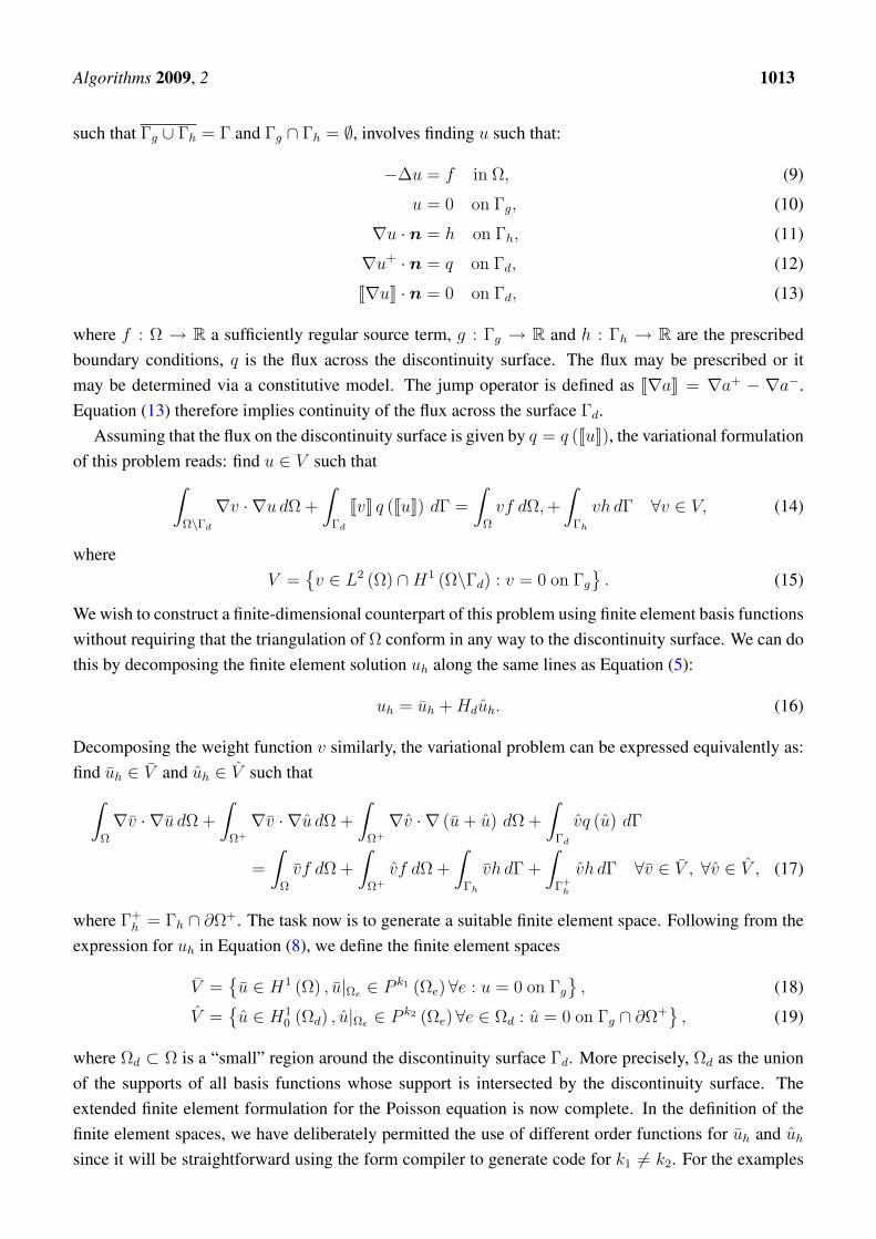
such that Γg ∪ Γh = Γ and Γg ∩ Γh = ∅, involves finding u such that:

−∆u = f in Ω, (9)

u = 0 on Γg, (10)

∇u · n = h on Γh, (11)

∇u+ · n = q on Γd, (12)

J∇uK · n = 0 on Γd, (13)

where f : Ω → R a sufficiently regular source term, g : Γg → R and h : Γh → R are the prescribedboundary conditions, q is the flux across the discontinuity surface. The flux may be prescribed or itmay be determined via a constitutive model. The jump operator is defined as J∇aK = ∇a+ − ∇a−.Equation (13) therefore implies continuity of the flux across the surface Γd.

Assuming that the flux on the discontinuity surface is given by q = q (JuK), the variational formulationof this problem reads: find u ∈ V such that∫

Ω\Γd

∇v · ∇u dΩ +

∫Γd

JvK q (JuK) dΓ =

∫Ω

vf dΩ,+

∫Γh

vh dΓ ∀v ∈ V, (14)

whereV =

v ∈ L2 (Ω) ∩H1 (Ω\Γd) : v = 0 on Γg

. (15)

We wish to construct a finite-dimensional counterpart of this problem using finite element basis functionswithout requiring that the triangulation of Ω conform in any way to the discontinuity surface. We can dothis by decomposing the finite element solution uh along the same lines as Equation (5):

uh = uh +Hduh. (16)

Decomposing the weight function v similarly, the variational problem can be expressed equivalently as:find uh ∈ V and uh ∈ V such that∫

Ω

∇v · ∇u dΩ +

∫Ω+

∇v · ∇u dΩ +

∫Ω+

∇v · ∇ (u+ u) dΩ +

∫Γd

vq (u) dΓ

=

∫Ω

vf dΩ +

∫Ω+

vf dΩ +

∫Γh

vh dΓ +

∫Γ+

h

vh dΓ ∀v ∈ V , ∀v ∈ V , (17)

where Γ+h = Γh ∩ ∂Ω+. The task now is to generate a suitable finite element space. Following from the

expression for uh in Equation (8), we define the finite element spaces

V =u ∈ H1 (Ω) , u|Ωe ∈ P k1 (Ωe)∀e : u = 0 on Γg

, (18)

V =u ∈ H1

0 (Ωd) , u|Ωe ∈ P k2 (Ωe)∀e ∈ Ωd : u = 0 on Γg ∩ ∂Ω+, (19)

where Ωd ⊂ Ω is a “small” region around the discontinuity surface Γd. More precisely, Ωd as the unionof the supports of all basis functions whose support is intersected by the discontinuity surface. Theextended finite element formulation for the Poisson equation is now complete. In the definition of thefinite element spaces, we have deliberately permitted the use of different order functions for uh and uh

since it will be straightforward using the form compiler to generate code for k1 6= k2. For the examples


presented in Section 5., it is assumed that k1 = k2 and that the solution goes to zero on the boundary,therefore we will use the compacter notation

V =vh ∈ L2 (Ω) ∩H1

0 (Ω\Γd) , vh|Ωe ∈ P k (Ωe\Γd)∀e

(20)

for a finite element function vh ∈ V , which is discontinuous across surfaces when defining the examples.The extended finite element problem can be expressed as a system of linear equations

Ku = f , (21)

which in an expanded format for the case q = k JuK, where k is a positive constant, reads[ ∫Ω

BTB dΩ

∫Ω+

dB

TB dΩ∫

Ω+d

BTB dΩ

∫Ω+

dB

TB dΩ +

∫Γd

NkN dΓ

][u

u

]=

[ ∫Ω

NTf dΩ∫

Ω+d

NTf dΩ

], (22)

where B and B contain derivatives of the shape functionsφi

and

φi

, respectively, N and N

contain shape functions, and u and u contain the degrees of freedom. Usually, the same finite elementbasis will be used for the regular and enriched components (k1 = k2 in Equations (18) and (19)), inwhich case B = B and N = N . Details of the matrix formulation and some practical aspects can befound in [19].

4. Automated Modelling of Discontinuities

The development of our automated approach for extended finite element methods can be broken downinto three keys parts. Firstly, the domain-specific language for variational forms which we have outlinedin Section 2. requires extension. It is necessary that finite element spaces with discontinuities acrosssurfaces can be represented and that terms can be evaluated and integrated on discontinuity surfaces.Secondly, the form compiler must be able to translate the high-level input into low-level computer codethat can perform the tasks required at the innermost assembly loop of a finite element program, namelycomputing the element matrices and vectors. For this, we have extended the form compiler FFC [6, 13].The third component is the solver. We have constructed a solver on top of the C++/Python libraryDOLFIN [7, 16]. It is at the solver level that discontinuity surfaces are represented, coefficients of finiteelement functions that appear in forms (such as w in the case of the weighted Poisson equation) aresupplied to the assembler and that the global system of linear equations is assembled and solved. Wedescribe each of the three key software library components in this section. The implementation of theform compiler and the solver components which support the extended finite element method are availablein the supporting material [12].

As already alluded, automated code generation offers a number of interesting possibilities. For ex-ample, it is possible to employ representations of finite element matrices and vectors which cannot bereasonably coded by hand. As an example, standard element matrices and vectors can be expressed usinga “tensor contraction” approach [6] which involves extensive “pre-computation” (prior to runtime), in-stead of the conventional quadrature-loop representation. Different representations can lead to dramaticdifferences in performance. The relative performance of different representations depends heavily on thenature of the differential Equation [6, 10]. At first inspection, for the extended finite element method we


are limited in terms of possible representations. This is due to the discontinuity surface being definedglobally in terms of the real coordinates, unlike shape functions which are usually defined on referencecells. This eliminates the possibility of using certain approaches, such as the tensor contraction ap-proach, which rely on all functions being defined on a reference element. Deeper inspections may yieldinteresting possibilities, but for now we limit ourselves to the automated generation of code which usesthe conventional quadrature representation. Even for quadrature representations, special optimisationsthrough automation can be applied, for example the automated rearrangement of loops which can havedramatic performance consequences beyond those which can be realised by modern generic compiler op-timisations [10]. Automation is particularly amenable to specialised performance optimisations, whichis not only because of the possibility of employing special strategies but also the simple regeneration ofthe code for a particular problem by following improvement to the form compiler.

4.1. Domain-Specific Language Extensions

In the domain-specific language used by the form compiler FFC, we need to include discontinuousfinite element function spaces, various operators at discontinuity surfaces and integration over disconti-nuity surfaces. Inspired by the decomposition of the displacement field in (5), we define “continuous”and “discontinuous” function spaces which will correspond to uh and uh, respectively, and a mixed spaceis then defined as the sum of the two,

elem_cont = FiniteElement(type, shape, order)

elem_discont = DiscontinuousFiniteElement(type, shape, order)

element = elem_cont + element_discont

where type is the finite element type e.g. “Lagrange”, “discontinuous Lagrange” (discontinuous acrosscell facets), or “Raviart-Thomas”, among others, shape defines the shape of the finite element cell(“interval”, “triangle” or “tetrahedron”) and order is the order of the finite element basis (which is arbi-trary). A finite element space which is suitable for modelling problems with discontinuous solutions hasbeen created from the sum of the continuous and discontinuous element spaces. Not all FFC supportedfinite element spaces are currently compatible with the extended finite element implementation. We willfocus on arbitrary order continuous Lagrange elements.

Once the finite element spaces have been defined, test, trial and other functions can be defined onthe appropriate spaces. For the Poisson equation presented in Section 3.2., we define the test and trialfunctions, v and u, respectively, and the source function f ,

v = TestFunctionPUM(element)

u = TrialFunctionPUM(element)

f = Function(elem_cont)

The test and trial functions have been defined on the space of functions containing a discontinuity andthe source function f is defined on a continuous finite element space.


FFC provides a number of operators for computing terms such as inner products, gradients, the diver-gence and the transpose [6, 7, 13]. It is possible to use compact tensor or index notation. In the contextof the extended finite element method, we define some operators which act at discontinuity surfaces.A common operation at a discontinuity surface is the computation of the jump in the field across thesurface. For this, we provide the operator djump(u) which is equivalent to u+ − u−, and the operatorljump(u, n) which returns the jump in the vector u+ − u−, but with the components of the jumprelative to the local n − s coordinate system in which the n-direction is normal to the discontinuitysurface and the s-direction is tangential to the discontinuity surface. Another ingredient is integrationover discontinuity surfaces which is denoted by *dc. The range of operators at discontinuity surfaces iscurrently limited. More elaborate operators, akin to those already available on cell facets [8], are underdevelopment.

We have now introduced the necessary language elements to represent a finite element variationalformulation of the Poisson problem with a discontinuous solution across a surface and a flux acting atthe discontinuity surface which is a function of the solution jump, as presented in Equation (14). For aquadratic Lagrange basis, and the constitutive model for the discontinuity surface flux q = k JuK wherek ≥ 0 is a constant, the form compiler input for this problem reads:

# Finite element spaces

elem_cont = FiniteElement("Lagrange", "triangle", 2)

elem_discont = DiscontinuousFiniteElement("Lagrange", "triangle", 2)

element = elem_cont + elem_discont

# Test and trial functions

v = TestFunctionPUM(element)

u = TrialFunctionPUM(element)

# Source term

f = Function(elem_cont)

# Interface flux parameter

k = Constant("triangle")

# Bilinear and linear forms

a = dot(grad(v), grad(u))*dx + k*djump(v)*djump(u)*dc

L = v*f*dx

The bilinear form is denoted by a and the linear form is denoted by L. The extended FFC can be calledfrom the command line to generate C++ code from this high-level input. The input to the form compilermirrors the mathematical formulation of the problem, thereby detaching the mathematical problem fromthe implementation details. This can dramatically reduce the time required to develop and test newmodels.


4.2. Specialised Generated Code

From the high-level input, low-level code which is specific to the considered equation is automati-cally generated by the form compiler. FFC generates C++ code which conforms to the Unified Form-assembly Code (UFC) specification [14, 15] (the generated code conforms to the upcoming version 1.2of UFC). The UFC specification is a C++ interface for the assembly of variational forms and provides aspecification against which automated code generators can work. An assembler that supports the UFCspecification can therefore assemble the global matrices and vectors from the generated code withoutmodification.

In the context of the extended finite element method, the computation of element matrices and vec-tors, and the degree of freedom maps are affected by the discontinuity surfaces. To exploit the UFCspecification, we follow a standard C++ polymorphic design and generate subclasses of the classes de-fined in the UFC specification. The automatically generated classes are initialised with a GenericPUMobject (the design of this object is described later in the section) which provides the data which is de-pendent on the presence of discontinuity surfaces and is necessary to build element matrices and vectorsfor the extended finite element method. The member functions of the generated code which are calledduring assembly are part of the UFC specification, which is why the global system of equations can beassembled by any assembly code which supports the specification. We outline some key elements of theautomatically generated code and describe their purpose. A number of other utility classes and functionsin addition to those which we will describe are also generated, such as functions for evaluating basisfunctions and their derivatives at arbitrary points.

The key classes generated by the form compiler address the degree of freedom maps, cell integrals(which include integration over a discontinuity surface within a cell) and forms, which represent mathe-matical variational forms. At the highest level of abstraction, given an object pum, forms are created. Forexample, for the Poisson equation, classes which represent the bilinear and linear forms are generated,

UFC_PoissonBilinearForm a(pum);

UFC_PoissonLinearForm L(pum);

Forms are self-aware of various properties, such as their rank, and are able to create the relevant degreeof freedom maps, integral objects and finite elements. Forms are the main interface through which anapplication developer interacts with the automatically generated code. A generated form is a subclass ofthe UFC class ufc::form. Typically, a form is passed together with a matrix/vector and a mesh to anassembler to build the global matrix/vector. A form object is also able to create degree of freedom maps(which are subclasses of the UFC class ufc::dof map). For the Poisson example, the form compilerwill generate code for a class from which an object is created by

Poisson_dof_map_0 dof_map(pum);

This object is able to tabulate the degree of freedom map for a given cell. The degree of freedom mapis aware of the discontinuity and the extra “enriched” degrees of freedom via the object pum. Degree of


freedom map classes can perform various tasks, as defined in the UFC specification. The numeral in theclass name is a convention in the generated code which indicates the particular degree of freedom map.Problems with multiple fields will involve multiple maps. However, the user is not exposed to this asthe degree of freedom maps are accessed via the higher-level form object. This naming convention isfollowed for other generated classes.

Objects which are able to compute an element matrix or vector are generated by the compiler and aresubclasses of ufc::cell integral from the UFC specification. A cell integral object for a Poissonproblem can be created by

Poisson_cell_integral_0 cell_integral(pum);

For each form that appears in a problem (usually there is one bilinear form and one linear form), therewill typically be a cell integral class. The key member function of the cell integral class is a “tabulate”function which computes the element matrix/vector. The tabulate function is supplied with a finite el-ement cell and any coefficient functions in the variational problem, and the element matrix or elementvector is computed. It is in the implementation of cell integrals and degree of freedom maps that aspectsof the extended finite element method in the generated code are most evident. The form compiler deter-mines the appropriate order of quadrature for an integral based on the operators and functions appearingin the form. There are also facilities for specifying the quadrature order manually.

In addition to code for computing degree of freedom maps and tabulating element matrices and vec-tors, tools which are useful for post-processing are also generated. Most prominent among these are toolsfor interpolating an extended finite element solution in a continuous space for visualisation purposes.

An important feature of the design of the generated code is that it is independent of the methodby which discontinuity surfaces are represented. This emphasises the separation of the mathematicaldefinition of the problem and implementation aspects.

At this stage, limited attention has been paid to specialised optimisations which are possible withautomated code generation. There may be considerable scope for this, as reported in [6, 10]. Automatedoptimisations are particularly pertinent to problems which involve multiple fields, possibly from differentfinite element spaces and which may or may not be discontinuous, as developing optimised code for suchproblems is difficult and time consuming.

4.3. Solver Environment

The key tasks of the solver environment are to make use of the generated code, provide representationsof discontinuity surfaces, and manage the local extension of the finite element function space and theresulting changes to the number of degrees of freedom. The solver is also responsible for a range ofstandard tasks, such as linear algebra data structures, linear solvers, application of Dirichlet boundaryconditions, mesh management and input/output. The necessary solver components are developed asextensions to the library DOLFIN [7, 16], which is designed to interact with automated code generators.The solver environment facilitates the use of generated code, therefore we provide an overview only.


Surface representation

Surfaces across which finite element functions are discontinuous are represented by the Surface

class. The interface to Surface is designed such that other parts of the library and the generated code areunaffected by the method with which a surface is represented internally. We presently work with simplerepresentations of surfaces, with the initial discontinuity surface represented by a mathematical function.This is not the most general approach as surfaces cannot “double back”, but it does permit a wide rangeof quite elaborate initial discontinuity paths to be considered. In two dimensions, a discontinuity surface(a line) is represented by a user-defined function and the start and end points. In three dimensions, thesurface is represented using two level set functions, φ and ψ, where for a point on the surface φ = 0

and ψ < 0. In both two and three dimensions, the functions used to describe the surface make use ofthe Function abstraction in DOLFIN. The interface to the class Surface is designed such that it isdimension-independent.

Once a Surface has been created, it can perform a range of geometric tasks, such as determining onwhich side of the surface a given point lies, finding the intersection point of a straight line and the surface,determining whether a cell is intersected by the surface and computing the ratio between the volumesof an intersected cell on either side of the surface. The design can be extended as extra functionallyis required. Multiple surfaces can be stored in standard STL containers, which is useful when dealingwith multiple discontinuities. When a crack grows, the surface object which represents the crack surfacesimply needs to be updated.

The Surface interface is not exposed in the generated code, which enforces the desirable separationbetween the generated code and the surface representation. Rather, only the GenericPUM interface,which is described below, is exposed in the generated code. Details of the surface representation can bechanged without disruption to other parts of the code. A user can define their own surface representationwithout needing to modify the form compiler.

Interface to the generated code and local extension of the finite element basis management

The local extension of the finite element basis is controlled by an object derived from the abstract baseclass GenericPUM. Its task is to manage aspects related to the partition of unity approach. The base classGenericPUM provides an interface for interacting with the generate code. Key tasks of a GenericPUM-based object include the evaluation of the Heaviside function at arbitrary points, computing quadratureschemes for intersected elements based on an input reference scheme which is provided by the generatedcode and managing which nodes have enriched functions attached. Each discontinuous field in a problemhas an associated GenricPUM object. For example, for a three-dimensional elasticity problem, there willbe a GenricPUM object associated with each of the three fields If GenricPUM objects are the same foreach field, then they can be shared. Partition of unity related data which is required by the generatedcode is accessed exclusively through the GenricPUM public interface.

For modelling discontinuities, we define an object PUM, which is a subclass of GenericPUM and isinitialised with the discontinuity surfaces, a mesh and the standard degree of freedom map (a map forthe standard degrees of freedom),


std::vector<const Surface*> surfaces;

PUM pum(surfaces, mesh, standard_dof_map);

When a discontinuity surface evolves, the PUM object simply needs to be updated to reflect the change.An important feature of GenericPUM-based objects is that the public interface is designed such that it

only involves arguments and return variables that are standard C++ types or part of the UFC specification.This is important as it allows a PUM object to act as the “glue” between the generated code and differentfinite element libraries. A user of any library which supports UFC can use the generated code by justproviding their own sub-class of GenericPUM.

To ensure that the jump in a solution goes to zero at the boundary of a discontinuity surface whichdoes not intersect the boundary of the domain, the enriched degrees of freedom are carefully selectedclose to the boundary of a discontinuity surface, as described in [19].

Function spaces and variational forms

We are now in a position to define function spaces and variational forms which are represented by theDOLFIN classes FunctionSpace and Form, respectively. A FunctionSpace represents the mathe-matical function space within which a solution is sought, such as those defined in Equation (20) whichdescribe the type of finite element functions. A FunctionSpace is also aware of the domain Ω and thedegree of freedom map (which in part defines the regularity of the function space). A Form is definedby the variational problem and the relevant function space(s). A Form can be assembled into a globalmatrix (in the case of a bilinear form) or a global vector (in the case of a linear form). These conceptsand abstractions are explained in detail in [7] for conventional finite element methods. For the Poissonproblem presented in Section 3.2., a function space, and bilinear and linear forms are created by

Poisson::FunctionSpace V(mesh, pum_objects);

Poisson::BilinearForm a(V, V);

Poisson::LinearForm L(V);

with the form objects being initialised with function spaces. The code for the above function spaceand form classes is generated by the form compiler. The form classes are essentially wrappers for theUFC PoissonBilinearForm and UFC PoissonLinearForm objects and are created to simply the in-teraction with the DOLFIN environment. For a problem with multiple fields, such as three-dimensionalincompressible elasticity, a PUM object is associated with each field (one for each displacement compo-nent plus one for the pressure field), therefore to create a function space we would have


std::vector<const GenericPUM*> pum_objects;

pum_objects.push_back(&pum_u);



pum_objects.push_back(&pum_p);

Incompressible3D::FunctionSpace V(mesh, pum_objects);

Since the displacement components are all discontinuous across the same surface and they share thesame finite element type, they can share the same PUM object. Usually the finite element field used forthe pressure field differs from that used for the displacement components, therefore it requires its ownPUM object. An incompressible elasticity formulation is elaborated in Section 5..

With the exception of Dirichlet boundary conditions, the finite element variational problem is com-pletely defined by the Form objects and the mesh. They can be passed to the assembler to compute theglobal matrix and vector.

Matrix A;

Vector b;

Assembler::assemble(A, a);

Assembler::assemble(b, L);

Once the global matrix and vector have been assembled, Dirichlet boundary conditions can be appliedto the linear system if necessary, and the system of linear equations can be solved as usual.

5. Examples

A number of examples are presented in this section to demonstrate various aspects of the automatedmodelling approach for simulating discontinuities. To avoid lengthy and intricate definitions of case-specific function spaces, the variational form of each example is presented for the case of homogeneousDirichlet boundary conditions, despite the computed problems using more elaborate boundary condi-tions. For each example we define the forms a and L, and the function space V . The form compilerinput is listed in this section for each example and the complete code for each example is available in thesupporting material [12]. All parameters which we use are non-dimensional.

The presented examples are linear, although the code generation approach can be used equally fornonlinear problems (see [7]).

5.1. Weighted Poisson Equation

We consider first the weighted Poisson with discontinuities in the solution u across the surfaces Γd andfluxes acting on the discontinuity surfaces. The bilinear and linear forms associated with this problem


read:

a (uh, vh) =

∫Ω\Γd

wh∇vh · ∇uh dΩ +

∫Γd

JvhK k JuhK dΓ, (23)

L (vh) =

∫Ω

vhf dΩ, (24)

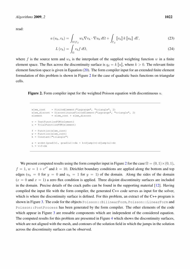
where f is the source term and wh is the interpolant of the supplied weighting function w in a finiteelement space. The flux across the discontinuity surface is qd = k JuK, where k > 0. The relevant finiteelement function space is given in Equation (20). The form compiler input for an extended finite elementformulation of this problem is shown in Figure 2 for the case of quadratic basis functions on triangularcells.

Figure 2. Form compiler input for the weighted Poisson equation with discontinuous u.

elem_cont = FiniteElement("Lagrange", "triangle", 2)elem_discont = DiscontinuousFiniteElement("Lagrange", "triangle", 2)element = elem_cont + elem_discont

v = TestFunctionPUM(element)u = TrialFunctionPUM(element)

f = Function(elem_cont)w = Function(elem_cont)k = Constant("triangle")

a = w*dot(grad(v), grad(u))*dx + k*djump(v)*djump(u)*dcL = v*f*dx

We present computed results using the form compiler input in Figure 2 for the case Ω = (0, 1)×(0, 1),f = 1, w = 1 + ex2 and k = 10. Dirichlet boundary conditions are applied along the bottom and topedges (uh = 0 for y = 0 and uh = 1 for y = 1) of the domain. Along the sides of the domain(x = 0 and x = 1) a zero flux condition is applied. Three disjoint discontinuity surfaces are includedin the domain. Precise details of the crack paths can be found in the supporting material [12]. Havingcompiled the input file with the form compiler, the generated C++ code serves as input for the solver,which is where the discontinuity surface is defined. For this problem, an extract of the C++ program isshown in Figure 3. The code for the objects Poisson::BilinearForm, Poisson::LinearForm andPoisson::PostProcess has been generated by the form compiler. The other elements of the codewhich appear in Figure 3 are reusable components which are independent of the considered equation.The computed results for this problem are presented in Figure 4 which shows the discontinuity surfaces,which are not aligned with the mesh, and contours of the solution field in which the jumps in the solutionacross the discontinuity surfaces can be observed.


Figure 3. C++ code extract for the two-dimensional weighted Poisson problem with discon-tinuities in the solution.

// Create function spacePoisson::FunctionSpace V(mesh, pum_objects);

// Create bilinear and linear FormsPoisson::BilinearForm a(V, V);a.k = k; a.w = w;Poisson::LinearForm L(V);L.f = f;

// Post processingPoisson::PostProcess post_process(mesh, pum_objects);

// Create a linear PDE variational problemdolfin::VariationalProblem pde(a, L, bcs);

// Solve pdedolfin::Function U(V);pde.solve(U);

// Interpolate solution for post processingdolfin::Function U_interpolated(V0);post_process.interpolate(U.vector(), U_interpolated.vector());

// Save solution and discontinuity surfaces to file for visualisationpum::VTKFile filep("surface.pvd");dolfin::File file("poisson.pvd");file << U_interpolated;filep << discontinuities;

Figure 4. Weighted Poisson problem in two dimensions: (a) mesh and discontinuity surfacesand (b) solution contours.

(a) (b)


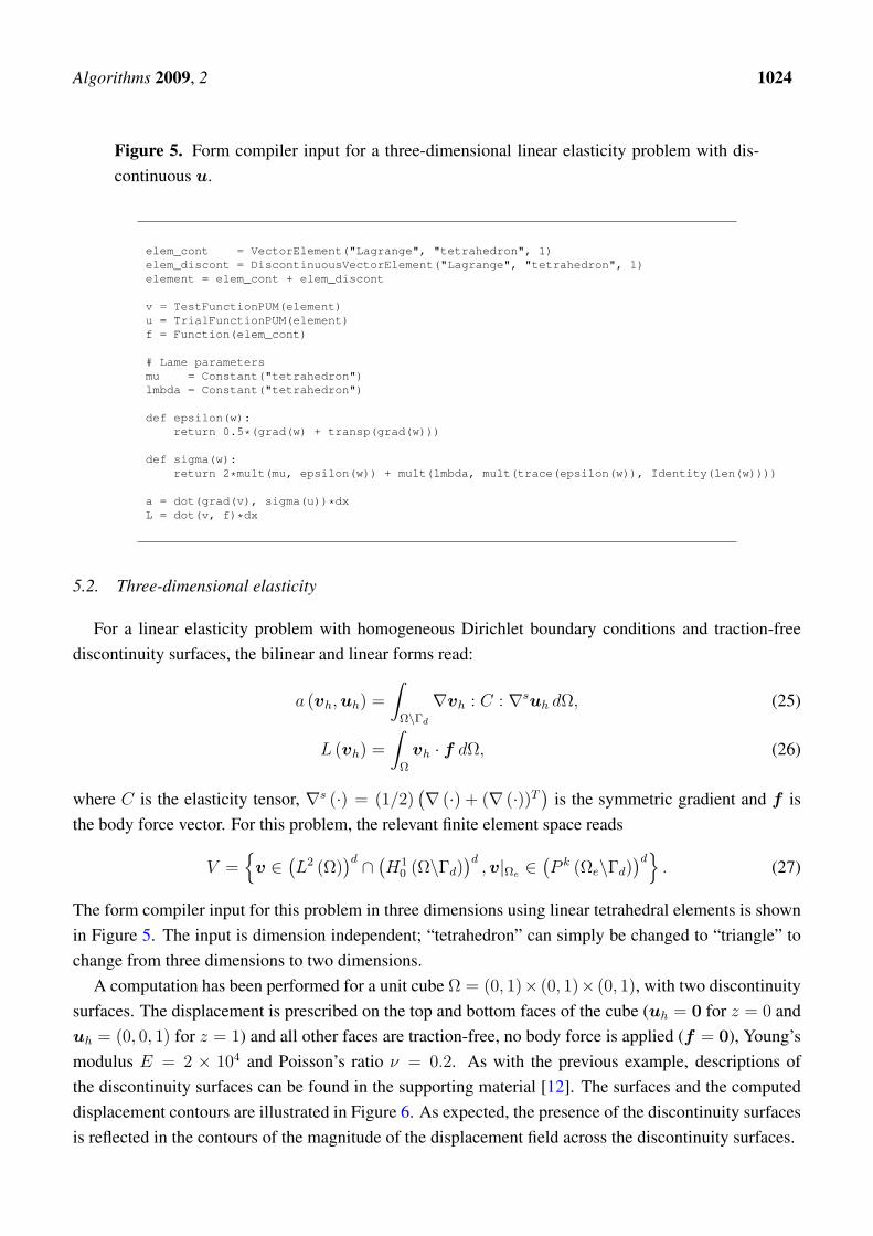
Figure 5. Form compiler input for a three-dimensional linear elasticity problem with dis-continuous u.

elem_cont = VectorElement("Lagrange", "tetrahedron", 1)elem_discont = DiscontinuousVectorElement("Lagrange", "tetrahedron", 1)element = elem_cont + elem_discont

v = TestFunctionPUM(element)u = TrialFunctionPUM(element)f = Function(elem_cont)

# Lame parametersmu = Constant("tetrahedron")lmbda = Constant("tetrahedron")

def epsilon(w):return 0.5*(grad(w) + transp(grad(w)))

def sigma(w):return 2*mult(mu, epsilon(w)) + mult(lmbda, mult(trace(epsilon(w)), Identity(len(w))))

a = dot(grad(v), sigma(u))*dxL = dot(v, f)*dx

5.2. Three-dimensional elasticity

For a linear elasticity problem with homogeneous Dirichlet boundary conditions and traction-freediscontinuity surfaces, the bilinear and linear forms read:

a (vh,uh) =

∫Ω\Γd

∇vh : C : ∇suh dΩ, (25)

L (vh) =

∫Ω

vh · f dΩ, (26)

where C is the elasticity tensor, ∇s (·) = (1/2)(∇ (·) + (∇ (·))T

)is the symmetric gradient and f is

the body force vector. For this problem, the relevant finite element space reads

V =

v ∈(L2 (Ω)

)d ∩ (H10 (Ω\Γd)

)d,v|Ωe ∈

(P k (Ωe\Γd)

)d. (27)

The form compiler input for this problem in three dimensions using linear tetrahedral elements is shownin Figure 5. The input is dimension independent; “tetrahedron” can simply be changed to “triangle” tochange from three dimensions to two dimensions.

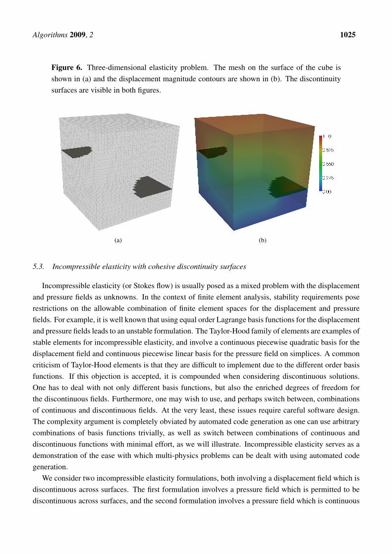
A computation has been performed for a unit cube Ω = (0, 1)× (0, 1)× (0, 1), with two discontinuitysurfaces. The displacement is prescribed on the top and bottom faces of the cube (uh = 0 for z = 0 anduh = (0, 0, 1) for z = 1) and all other faces are traction-free, no body force is applied (f = 0), Young’smodulus E = 2 × 104 and Poisson’s ratio ν = 0.2. As with the previous example, descriptions ofthe discontinuity surfaces can be found in the supporting material [12]. The surfaces and the computeddisplacement contours are illustrated in Figure 6. As expected, the presence of the discontinuity surfacesis reflected in the contours of the magnitude of the displacement field across the discontinuity surfaces.


Figure 6. Three-dimensional elasticity problem. The mesh on the surface of the cube isshown in (a) and the displacement magnitude contours are shown in (b). The discontinuitysurfaces are visible in both figures.

(a) (b)

5.3. Incompressible elasticity with cohesive discontinuity surfaces

Incompressible elasticity (or Stokes flow) is usually posed as a mixed problem with the displacementand pressure fields as unknowns. In the context of finite element analysis, stability requirements poserestrictions on the allowable combination of finite element spaces for the displacement and pressurefields. For example, it is well known that using equal order Lagrange basis functions for the displacementand pressure fields leads to an unstable formulation. The Taylor-Hood family of elements are examples ofstable elements for incompressible elasticity, and involve a continuous piecewise quadratic basis for thedisplacement field and continuous piecewise linear basis for the pressure field on simplices. A commoncriticism of Taylor-Hood elements is that they are difficult to implement due to the different order basisfunctions. If this objection is accepted, it is compounded when considering discontinuous solutions.One has to deal with not only different basis functions, but also the enriched degrees of freedom forthe discontinuous fields. Furthermore, one may wish to use, and perhaps switch between, combinationsof continuous and discontinuous fields. At the very least, these issues require careful software design.The complexity argument is completely obviated by automated code generation as one can use arbitrarycombinations of basis functions trivially, as well as switch between combinations of continuous anddiscontinuous functions with minimal effort, as we will illustrate. Incompressible elasticity serves as ademonstration of the ease with which multi-physics problems can be dealt with using automated codegeneration.

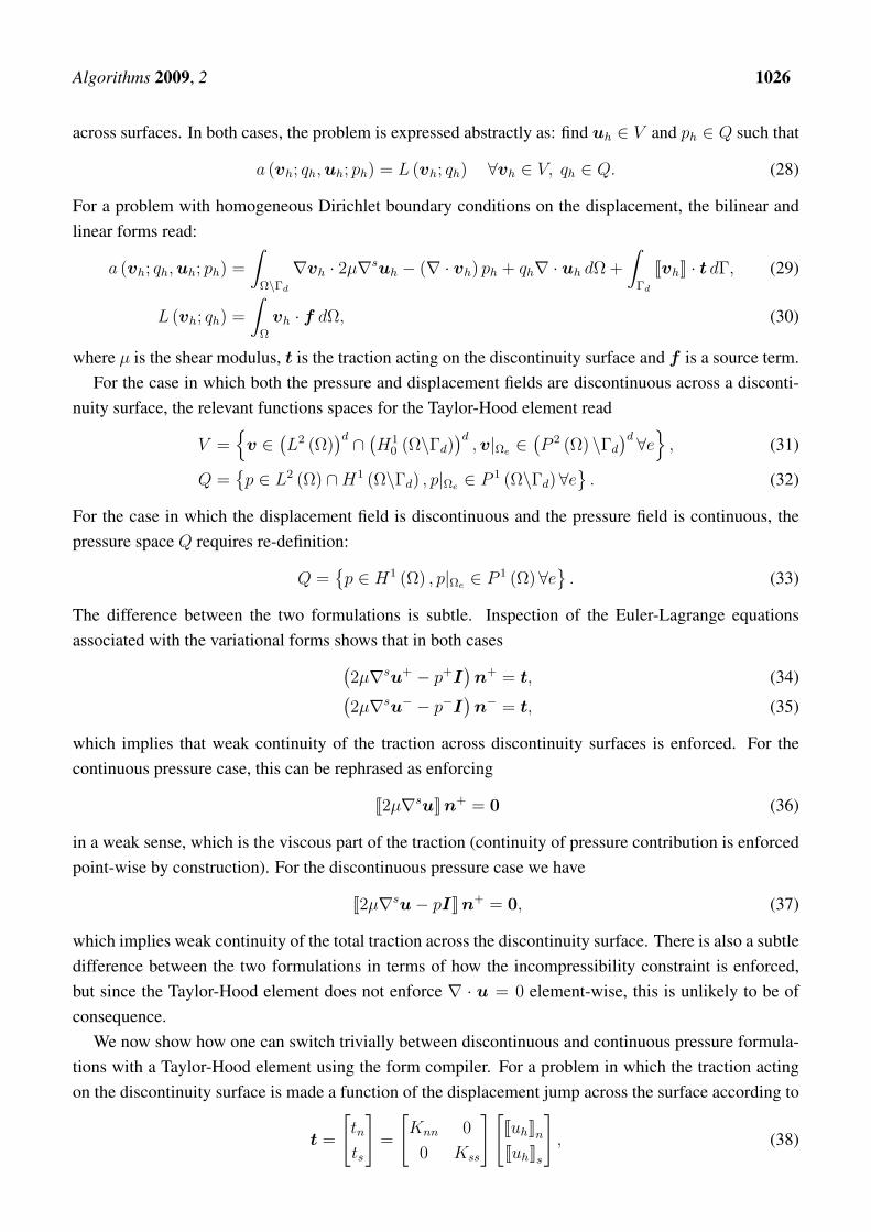
We consider two incompressible elasticity formulations, both involving a displacement field which isdiscontinuous across surfaces. The first formulation involves a pressure field which is permitted to bediscontinuous across surfaces, and the second formulation involves a pressure field which is continuous


across surfaces. In both cases, the problem is expressed abstractly as: find uh ∈ V and ph ∈ Q such that

a (vh; qh,uh; ph) = L (vh; qh) ∀vh ∈ V, qh ∈ Q. (28)

For a problem with homogeneous Dirichlet boundary conditions on the displacement, the bilinear andlinear forms read:

a (vh; qh,uh; ph) =

∫Ω\Γd

∇vh · 2µ∇suh − (∇ · vh) ph + qh∇ · uh dΩ +

∫Γd

JvhK · t dΓ, (29)

L (vh; qh) =

∫Ω

vh · f dΩ, (30)

where µ is the shear modulus, t is the traction acting on the discontinuity surface and f is a source term.For the case in which both the pressure and displacement fields are discontinuous across a disconti-

nuity surface, the relevant functions spaces for the Taylor-Hood element read

V =

v ∈(L2 (Ω)

)d ∩ (H10 (Ω\Γd)

)d,v|Ωe ∈

(P 2 (Ω) \Γd

)d ∀e , (31)

Q =p ∈ L2 (Ω) ∩H1 (Ω\Γd) , p|Ωe ∈ P 1 (Ω\Γd)∀e

. (32)

For the case in which the displacement field is discontinuous and the pressure field is continuous, thepressure space Q requires re-definition:

Q =p ∈ H1 (Ω) , p|Ωe ∈ P 1 (Ω)∀e

. (33)

The difference between the two formulations is subtle. Inspection of the Euler-Lagrange equationsassociated with the variational forms shows that in both cases(

2µ∇su+ − p+I)n+ = t, (34)(

2µ∇su− − p−I)n− = t, (35)

which implies that weak continuity of the traction across discontinuity surfaces is enforced. For thecontinuous pressure case, this can be rephrased as enforcing

J2µ∇suK n+ = 0 (36)

in a weak sense, which is the viscous part of the traction (continuity of pressure contribution is enforcedpoint-wise by construction). For the discontinuous pressure case we have

J2µ∇su− pIK n+ = 0, (37)

which implies weak continuity of the total traction across the discontinuity surface. There is also a subtledifference between the two formulations in terms of how the incompressibility constraint is enforced,but since the Taylor-Hood element does not enforce ∇ · u = 0 element-wise, this is unlikely to be ofconsequence.

We now show how one can switch trivially between discontinuous and continuous pressure formula-tions with a Taylor-Hood element using the form compiler. For a problem in which the traction actingon the discontinuity surface is made a function of the displacement jump across the surface according to

t =

[tn

ts

]=

[Knn 0

0 Kss

][JuhKn

JuhKs

], (38)


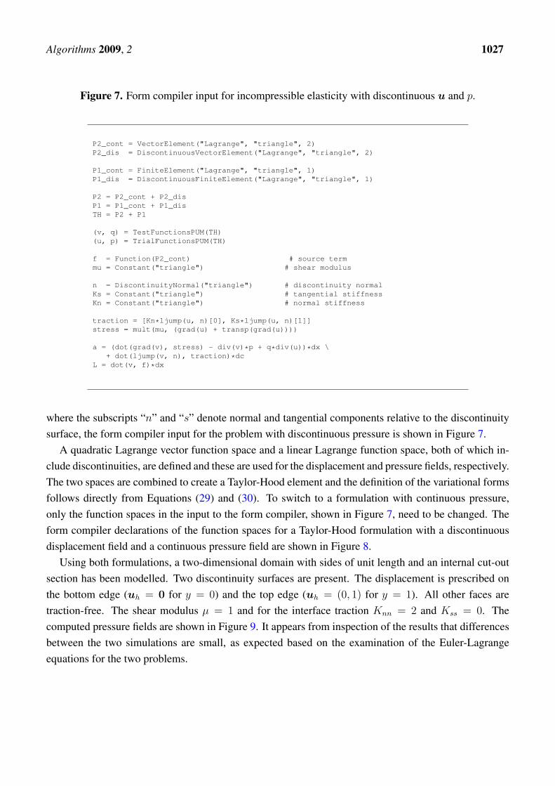
Figure 7. Form compiler input for incompressible elasticity with discontinuous u and p.

P2_cont = VectorElement("Lagrange", "triangle", 2)P2_dis = DiscontinuousVectorElement("Lagrange", "triangle", 2)

P1_cont = FiniteElement("Lagrange", "triangle", 1)P1_dis = DiscontinuousFiniteElement("Lagrange", "triangle", 1)

P2 = P2_cont + P2_disP1 = P1_cont + P1_disTH = P2 + P1

(v, q) = TestFunctionsPUM(TH)(u, p) = TrialFunctionsPUM(TH)

f = Function(P2_cont) # source termmu = Constant("triangle") # shear modulus

n = DiscontinuityNormal("triangle") # discontinuity normalKs = Constant("triangle") # tangential stiffnessKn = Constant("triangle") # normal stiffness

traction = [Kn*ljump(u, n)[0], Ks*ljump(u, n)[1]]stress = mult(mu, (grad(u) + transp(grad(u))))

a = (dot(grad(v), stress) - div(v)*p + q*div(u))*dx \+ dot(ljump(v, n), traction)*dc

L = dot(v, f)*dx

where the subscripts “n” and “s” denote normal and tangential components relative to the discontinuitysurface, the form compiler input for the problem with discontinuous pressure is shown in Figure 7.

A quadratic Lagrange vector function space and a linear Lagrange function space, both of which in-clude discontinuities, are defined and these are used for the displacement and pressure fields, respectively.The two spaces are combined to create a Taylor-Hood element and the definition of the variational formsfollows directly from Equations (29) and (30). To switch to a formulation with continuous pressure,only the function spaces in the input to the form compiler, shown in Figure 7, need to be changed. Theform compiler declarations of the function spaces for a Taylor-Hood formulation with a discontinuousdisplacement field and a continuous pressure field are shown in Figure 8.

Using both formulations, a two-dimensional domain with sides of unit length and an internal cut-outsection has been modelled. Two discontinuity surfaces are present. The displacement is prescribed onthe bottom edge (uh = 0 for y = 0) and the top edge (uh = (0, 1) for y = 1). All other faces aretraction-free. The shear modulus µ = 1 and for the interface traction Knn = 2 and Kss = 0. Thecomputed pressure fields are shown in Figure 9. It appears from inspection of the results that differencesbetween the two simulations are small, as expected based on the examination of the Euler-Lagrangeequations for the two problems.


Figure 8. Function space definitions for the form compiler input for incompressible elasticitywith discontinuous u and continuous p. The definition of the functions and forms is identicalto that in Figure 7.

P2_cont = VectorElement("Lagrange", "triangle", 2)P2_dis = DiscontinuousVectorElement("Lagrange", "triangle", 2)

P1 = FiniteElement("Lagrange", "triangle", 1)

P2 = P2_cont + P2_disTH = P2 + P1

Figure 9. Pressure fields for (a) the continuous pressure case and (b) the discontinuouspressure case.

(a) (b)

6. Conclusions

We have demonstrated an automated code generation approach for the extended finite element method.A domain-specific language has been extended so that the equation of interest, in a variational format,can be expressed in a high-level language, and low-level C++ code is automatically generated throughthe form compiler. The approach facilitates the rapid development of new models that involve disconti-nuities and provides scope for special optimisations not tractable by hand. Furthermore, expressing theequation of interest in an abstract form provides separation between the considered model (the differ-ential equation and the function spaces) and aspects of the implementation. In practice, the approachreduces the implementation burden for developers. A number of concrete examples have been presentedin which problems that involve multiple fields with different finite element bases are addressed. Theinput language is extensible, so a wider range of discontinuity-specific operators can be developed todeal with a wider range of problems.


Acknowledgements

MN acknowledges the support of the Netherlands Technology Foundation STW, the NetherlandsOrganisation for Scientific Research and the Ministry of Public Works and Water Management.

References and Notes

1. Melenk, J. M.; Babuska, I. The partition of unity finite element method: Basic theory and applica-tions. Comput. Method. Appl. Mech. Eng. 1996, 139, 289–314.

2. Moes, N.; Dolbow, J.; Belytschko, T. A finite element method for crack growth without remeshing.Int. J. Numer. Method. Eng. 1999, 46, 231–150.

3. Belytschko, T.; N. Moes, S. U.; Parimik, C. Arbitrary discontinuities in finite elements. Int. J.Numer. Method. Eng. 2001, 50, 993–1013.

4. Strouboulis, T.; Copps, K.; Babuska, I. The generalized finite element method. Comput. Method.Appl. Mech. Eng. 2001, 190, 4081 – 4193.

5. Bordas, S.; Nguyen, P. V.; Dunant, C.; Guidoum, A.; Nguyen-Dang, H. An extended finite elementlibrary. Int. J. Numer. Method. Eng. 2007, 71, 703–732.

6. Kirby, R. C.; Logg, A. A compiler for variational forms. ACM Trans. Math. Software 2006,32, 417–444.

7. Logg, A.; Wells, G. N. DOLFIN: Automated finite element modelling, 2009. Available online:http://www.dspace.cam.ac.uk/handle/1810/214787.

8. Ølgaard, K. B.; Logg, A.; Wells, G. N. Automated code generation for discontinuous Galerkinmethods. SIAM J. Sci. Comput. 2008, 31, 849–864.

9. Rognes, M. E.; Kirby, R. C.; Logg, A. Efficient assembly of H(div) and H(curl) conforming finiteelements 2009. Submitted.

10. Ølgaard, K. B.; Wells, G. N. Optimisations for quadrature representations of finite element tensorsthrough automated code generation. ACM Trans. Math. Software 2010, 37. Available online:http://www.dspace.cam.ac.uk/handle/1810/218613.

11. FEniCS. FEniCS Project 2009. Available online: http://www.fenics.org/.12. Nikbakht, M.; Wells, G. N. Supporting material 2009. Available online: http://www.dspace.cam.

ac.uk/handle/1810/218650.13. Logg, A.; others. FEniCS Form Compiler 2009. Available online: http://www.fenics.org/ffc.14. Alnæs, M. S.; Logg, A.; Mardal, K.-A.; Skavhaug, O.; Langtangen, H. P. UFC Specification User

Manual, 2009. Available online: http://www.fenics.org/ufc/.15. Alnæs, M. S.; Logg, A.; Mardal, K.-A.; Skavhaug, O.; Langtangen, H. P. Unified framework for

finite element assembly. Int. J. Computat. Sci. Eng. 2009. Available online: http://simula.no/research/scientific/publications/Simula.SC.96/simula pdf file.

16. Logg, A.; Wells, G. N.; others. DOLFIN 2009. Available online: http://www.fenics.org/dolfin.17. Babuska, I.; Melenk, J. M. The Partition of Unity Method. Int. J. Numer. Method. Eng. 1997,

40, 727–758.18. Belytschko, T.; Black, T. Elastic crack growth in finite elements with minimal remeshing. Int. J.

Numer. Method. Eng. 1999, 45, 601–620.

http://www.dspace.cam.ac.uk/handle/1810/214787


http://www.fenics.org/



http://www.fenics.org/ffc

http://www.fenics.org/ufc/

http://simula.no/research/scientific/publications/Simula.SC.96/simula_pdf_file

http://simula.no/research/scientific/publications/Simula.SC.96/simula_pdf_file

http://www.fenics.org/dolfin


19. Wells, G. N.; Sluys, L. J. A new method for modelling cohesive cracks using finite elements. Int.J. Numer. Method. Eng. 2001, 50, 2667–2682.

c© 2009 by the authors; licensee Molecular Diversity Preservation International, Basel, Switzerland.This article is an open-access article distributed under the terms and conditions of the Creative CommonsAttribution license (http://creativecommons.org/licenses/by/3.0/).

Automated Modelling of Evolving Discontinuities

Documents

Transcript of Automated Modelling of Evolving Discontinuities