RANDOM JUMPS IN EVOLVING RANDOM ENVIRONMENT

C. BoldrighiniDipartimento di Matematica G. Castelnuovo, Universita ”La Sapienza”, Piazzale Aldo

Moro 2, 00185 Roma, Italy.Partially supported by INdAM (G.N.F.M.) and M.U.R.S.T. research funds.

Yu. G. KondratievDepartment of Mathematics, Bielefeld University, 33615 Bielefeld, Germany.

R. A. MinlosInstitute for Problems of Information Transmission, Russian Academy of Sciences.Partially supported by INdAM (G.N.F.M.) and M.U.R.S.T. research funds, by RFFI

grants n. 05-01-00449, Scientific School grant n. 934.2003.1, and CRDF research funds NRM1-2085.

A. PellegrinottiDipartimento di Matematica, Universita di Roma Tre, Largo San Leonardo Murialdo

1, 00146 Roma, Italy.Partially supported by INdAM (G.N.F.M.) and M.U.R.S.T. research funds.

E. A. ZhizhinaInstitute for Problems of Information Transmission, Russian Academy of Sciences.Partially supported by RFFI grants n. 05-01-00449, Scientific School grant n. 934.2003.1.

Abstract. We consider a particle moving in Rd accordingly to a jump Markov processand interacting with an evolving random environment. The latter is represented by a sta-tionary Glauber type dynamics in the continuum. Assuming a low activity-high temperatureregime for the Glauber dynamics and small coupling between particle and environment, weobtain the large time asymptotics for the particle position distribution.

AMS Mathematics Subject Classification: 60K35, 60J75, 60J80, 82C21, 82C22

Keywords: Jump Markov processes; Birth-and-death process; Continuous system; Gibbsmeasure; Glauber dynamics; Random environment.

§1. Introduction and main results.

In this paper we study the asymptotics for large time of the distribution of the positionof a tagged particle in Rd interacting with other particles, described by a random Markovpoint field in Rd. For this field we assume that it is a stationary birth-and-death Markovprocess, namely, the equilibrium Glauber type stochastic dynamics of a gas of particles,which was studied in [8, 11].

The study of the asymptotic behavior of lattice random walks in random environmentsis a quite well developed area of modern Mathematical Physics and stochastics. (See [3,4]for the case of evolving environment. For the problem of fixed environment, which is much

1

more studied, we refer to the recent review [15].) The main novelty of the present paperconsists in considering a continuous space random walk in interacting with an equilibriumMarkov process on a continuous configuration space.

Passing to precise definitions, we take as state space of the model Rd ×Γ, where Rd isthe state space of the tagged particle, and Γ, the state space of the random environment,is the space of all locally finite configurations of points in Rd.

The free random walk of the tagged particle is a jump Markov process in Rd startingfrom a given position x0 ∈ Rd. The intensity of the jumps from x to y is given by anonnegative function a(x − y) ≥ 0, which we assume to be even, continuous, and fastdecreasing at infinity. The generator of the corresponding stochastic semigroup of theprocess is a self-adjoint operator in L2(Rd) of the form

(LRW f)(x) =∫

Rd

a(x − y)(f(y) − f(x))dy, f ∈ L2(Rd). (1.1)

The Fourier transform of the function a,

a(λ) =∫

Rd

a(u) ei(λ,u) du, λ ∈ Rd, (1.2)

is an even real function, and satisfies the relation |a(λ)| ≤ a(0). Moreover

|a(λ)| < a(0) λ �= 0, (1.3a)

and the Taylor expansions of a(λ) in a neighborhood of λ = 0 is of the form

a(λ) = a(0) − 12

d∑i,j=1

aijλiλj + O(|λ|4), (1.3b)

where the matrix A = {aij} is positive definite.

The free evolution of the random environment is a birth-and-death Markov processwith state space Γ. The particles do not move, they only randomly appear and disappearin Rd. A particle configuration (a point of Γ) is denoted γ. The rates of the process (seefor more detail [2,11]) are

d(x, γ) ≡ 1 for death of a particle at x ∈ γ (1.4a)

b(x, γ) = ze−β

∑y∈γ

φ(x−y) for birth of a particle at x ∈ Rd. (1.4b)

φ is an even interaction potential between particles. The activity z and the inverse tem-perature β are the parameters of the model.

The corresponding stationary Markov process {γt : t ∈ R1} with the rates (1.4a,b) wasconstructed in [11, 12], where it was also shown that the stationary measures are Gibbsianmeasures µβ,z generated by the formal Hamiltonian

H(γ) =∑

x,y∈γ

φ(x − y)

2

with parameters β, z.We now formulate general assumptions on the parameters β, z and the potential φ

which guarantee existence and uniqueness of the Gibbs measures µβ,z.

1. Integrability.

C(β) =∫

Rd

|1 − e−βφ(u)|du < +∞ for any β > 0 (1.5a)

2. Positivity.φ(u) ≥ 0 u ∈ Rd (1.5b)

3. Low activity-high temperature regime. We assume that z and β are such that

ε := zC(β) << 1, (1.5c)

i.e., we assume that ε is small enough.

The generator of the process {γt} acting on L2(Γ, µβ,z) has the form

(LREF )(γ) =∑x∈γ

(F (γ \ x) − F (γ)) + z

∫Rd

e−β

∑y∈γ

φ(x−y)(F (γ ∪ x) − F (γ))dx (1.6)

The operator LRE is defined on the set of the bounded local functions and under ourassumptions is an essentially self-adjoint operator in L2(Γ, µβ,z) (see details in [11]).

The interaction of the tagged particle with the random environment is given by a termwhich modulates the intensity of the jumps of the particle in dependence of the field:

a(x − y)

(1 + κ

∑u∈γ

p(x − u)

). (1.7)

Here κ is a constant which will be assumed to be small enough, and the function p(u) iscontinuous, nonnegative, even, bounded and rapidly decreasing at infinity. Observe thatsuch interaction implies that the particle moves faster in regions with high concentrationof points of the environment. We set

p0 := maxu

p(u) < ∞, p1 :=∫

Rd

p(u)du. (1.8)

The first result to prove is an existence theorem.Theorem 1.1. Under the assumptions above on the functions a(u), p(u), the constant

κ, and (1.5,a,b,c) on φ, β and z, for a.a. choices of the initial data (x0, γ0), with respectto the measure dx0 × dµβ,z(γ0), there is a Markov process {(Xt, γt), t ≥ 0} on the space

3

Rd × Γ starting at (x0, γ0) . The generator of the corresponding stochastic semigroup S(t)on H = L2(Rd) ⊗ L2(Γ, µβ,z) is

(LF )(x, γ) = ((LRW ⊗ I2)F )(x, γ) + κ

∫Rd

a(x − y)∑u∈γ

p(x − u)(F (y, γ) − F (x, γ)) dy

+ ((I1 ⊗ LRE)F )(x, γ) (1.9)

where I1 and I2 are the identity operators in L2(Rd) and L2(Γ, µβ,z) = L2(Γ) respectively.

Theorem 1.1 is a particular case of a general problem of constructing processes fora system consisting of a particle in interaction with an equilibrium field. The proof isnecessarily rather lengthy, and will be fully published in a separate paper. Here we giveonly a sketch, which deals with a central point for the existence problem, that of obtaininga convenient bound on the number of jumps of the particle.

Sketch of the proof. We will prove that the number of jumps in any finite time in-terval is a.e. finite under some simplifying assumptions, namely that the function a(·), p(·),defined in (1.1), 1.7), are finite range (without loss of generality we may assume that theyhave the same range r > 0).

Let γs : s ∈ [0, T ) be a trajectory of the environment, and {(X0, 0), (X1, t1), . . . } be atrajectory of the random walk. It is easy to see that the positions X0, X1, . . . are a Markovchain with transition probabilities P (Xn = xn|Xn−1 = xn−1) = a(0)−1a(xn − xn−1). Thejump time at position x ∈ Rd at time s ∈ R+ has intensity

λ(x, γs) = a(0)

(1 + κ

∑u∈γs

p(x − u)

).

To prove that the random walk is well defined for a.a. trajectories of the environment weneed to prove that the number of jumps is finite in any fixed time interval [0, T ).

We do this by constructing a random walk with the same trajectories, and intensitiesλT (x), which depend on the set of births of the trajectory γs, s ∈ [0, T ), and are such thatλT (x) ≥ λ(x, γs) for all s ∈ [0, T ). We then prove that for any random walk trajectory∑∞

j=0 λ−1T (Xj) = ∞, which implies (see [5]) a finite number of jumps up to time T for the

process with rates λT (x). The proof will follow by a simple coupling between the latterprocess and the original one.

In fact, consider a pure birth process with intensity z ≥ supx,γ b(x, γ) starting fromthe initial configuration γ0. Denoting the new process by γ, by a trivial coupling, whichshould be such that the births of γ are a subset of the births of γ, we have γ(s) ⊆ γ(s),almost-surely for any s ∈ R+. As γs1 ⊆ γs2 for all s1 < s2, we have, for all s ∈ [0, T ),γ(s) ⊆ γT = γ(0) ∪ γT , where γT is a Poisson process with intensity zT . Therefore

λ(x, γ(s)) ≤ λ(x, γT ) = a(0)−1

1 + κ∑

u∈γT

p(x − u)

:= λT (x), (1.10a)

for all s ∈ [0, T ). By a result of the paper [10] we have, a.s., the following bound

|γT ∩ B(x, r)| ≤ CγT(r) ln(2 + |x|), (1.10b)

4

where B(x, r) is the ball with center x ∈ Rd and radius r > 0 and CγT(r) is a constant

independent of x. Therefore by (1.10a,b) we have

λT (x) ≤ a(0)−1 (1 + κp0CγT(r) ln(2 + |x|)) .

As a(·) is finite range, |λT (Xn)| ≤ a(0)−1 + CγTln(2 + nr), so that

∑∞j=0 λ−1(Xj) = ∞.

The original random walk can be coupled to the random walk with intensities λT (x)in such a way that the trajectories are the same and at each site of these trajectories theoriginal random walk leaves the site not earlier than the new random walk.

To do this, consider that for a fixed trajectory, the random walk can be determinedby assigning to each site x a Poisson process in [0,∞) which gives the jump times. Forthe original random walk this is process πx(s) with intensity λ(x, γs), depending on time,and for the new one it is a process πT

x (s) with constant intensity λT (x). We now, foreach x in the given trajectory, couple the processes πx(s) and πT

x (s) in such a way thatthe realizations of the first one are a subset of the realizations of the second one (whichis possible because λ(x, γs) < λT (x)). Then the original random walk leaves the startingpoint x0 not earlier than the new one, and the same clearly happens at all the subsequentpoints of the trajectory. Hence the number of jumps of the original random walk is alwaysless than the number of jumps of the new one.

We introduce the normalized displacement ut = Xt−x0√t

, and for any bounded regionG ⊂ Rd with piecewise smooth boundary, we consider the probability

Pr (ut ∈ G|X0 = x0) =∫

dµβ,z(γ0)∫

IG(ut) dP (Xt, γt|X0, γ0)

=∫

(S(t)ΦG)(x0, γ0)dµβ,z(γ0), (1.11)

where ΦG(u, γ) = IG(u), IG is the indicator function of the region G, and P (Xt, γt|X0, γ0)is the conditional distribution of the process (Xt, γt) at time t under the condition thatthe initial state is fixed. We want to study the limit of the probability (1.11) as t → ∞.

Theorem 1.2. Under the conditions above, for κ and ε small enough the limit of theprobability (1.11) exists and is given by

limt→∞

Pr (ut ∈ G|X0 = x0) =1

(2π)d2

√det A

∫G

e−12 (A−1ξ,ξ)dξ. (1.12a)

Here A = {aij} is a real symmetric positive definite matrix, with elements verifying thefollowing estimates

maxi,j

|aij − aij | < C ε, (1.12b)

where the matrix {aij} is defined by (1.3b), C is an absolute positive constant and ε isgiven by (1.5c).

5

In what follows we first consider the asymptotics for a more general quantity. Let ϕbe a bounded function on Rd. Consider the average

E (ϕ(ut)|X0 = x0) =∫

Γ

(S(t)Φϕ) (x0, γ0)dµβ,z(γ0) (1.13)

where Φϕ(u, γ) = ϕ(u). We first prove that the limit of the quantity E(ϕ(ut)|X0 = x0) ast → ∞ exists for a sufficiently regular function ϕ and is given by

limt→∞

E (ϕ(ut)|X0 = x0) =1

(2π)d2

√det A

∫Rd

e−12 (A−1ξ,ξ)ϕ(ξ)dξ. (1.14)

From this result we then deduce the assertion of Theorem 1.2.

It would be of course interesting to consider as environment process some other Markovprocesses on the configuration space, such as equilibrium Kawasaki dynamics in the con-tinuum, see [12]. But the problem is that in order to apply the approach developed inour paper one needs first of all a careful analysis of the spectral properties of the envi-ronment process. The latter was done in [8] for the case of the Glauber type dynamicsin the continuum and this information is used in an essential way in the present paper.Taking into consideration other types of equilibrium infinite particle processes will need,as a preliminary step, an analogous spectral analysis of their generators.

§2. Preliminary constructions.

2.1. Decompositions according to the eigenspaces of the translation group.

We denote the translation operators in H by Vs, s ∈ Rd:

(Vsf)(x, γ) = f(x + s, γ + s), f ∈ H, s ∈ Rd, (2.1)

where γ +s = {u+s : u ∈ γ} denotes, as usual, the space shift of γ. We have the canonicalisomorphism

T : H →∫

Rd

Hλdλ (2.2)

and the space Hλ can be identified with the space L2(Γ, µβ,z), and T acts according to theformula

(TΦ)λ(γ) =∫

Rd

Φ(x, γ + x) ei(λ,x)dx := Φλ(γ), Φ ∈ H. (2.3a)

Clearly, the action of the group Vs on Hλ reduces to multiplication by e−i(λ,s), i.e.,

(TVsΦ)λ(γ) = e−i(λ,s)Φλ(γ). (2.3b)

The inverse transformation T−1 acts according to the formula(T−1Φλ

)(x, γ) =

1(2π)d

∫Rd

Φλ(γ − x)e−i(λ,x)dλ. (2.4)

6

The operators L and S(t) commute with the translation group and are decomposedby the decomposition of the space (2.2), i.e.,

L =∫

Rd

Lλdλ, S(t) =∫

Rd

Sλ(t)dλ,

where the operators Lλ and Sλ(t) for λ ∈ Rd act on Hλ, i.e., in L2(Γ, µβ,z). Moreover theoperators {Sλ(t), t ≥ 0} form a semigroup with generator Lλ given by

(LΦ)λ(γ) =∫

Rd

a(u)(Φλ(γ + u)ei(λ,u) − Φλ(γ)

)du +

∑y∈γ

(Φλ(γ \ {y}) − Φλ(γ)) +

z

∫e−β

∑y∈γ

φ(u−y)(Φλ(γ ∪ {u}) − Φλ(γ))du +

κ∑v∈γ

p(v)∫

a(u)(Φλ(γ + u)ei(λ,u) − Φλ(γ)

)du := (LλΦλ)(γ). (2.5)

2.2. Spectrum of the ”free” (unperturbed) generator.

In what follows we will deduce Theorem 1.2 by the analysis of the upper branch ofthe spectrum of the full generator L. However for a better understanding of the picture ofsuch spectrum we first study the spectrum of the unperturbed generator (for κ = 0)

L(0) = LRW ⊗ I2 + I1 ⊗ LRE (2.6)

where I1, I2 are the identity operators in the spaces L2(Rd) and L2(Γ, µβ,z), respectively.Let by us, Us be the unitary shift operators on L2(Rd) and L2(Γ, µβ,z), respectively:

(usf)(x) = f(x + s), (UsΦ)(γ) = Φ(γ + s).

As it follows immediately from formula (1.1), by Fourier transform the operators LRW

and us go into multiplication operators, respectively, by the functions e0(λ) := a(λ)− a(0)and e−i(λ,s), acting on L2(Rd). Therefore the spectrum of LRW is the whole interval[minλ e0(λ), 0].

The spectrum of LRE in L2(Γ, µβ,z) (more precisely, its upper branch), was extensivelystudied in the paper [8]. We briefly recall the results. The operator LRE has the followingproperties.

1. It has an eigenvector Φ0 ≡ 1 with eigenvalue 0. We denote by h0 = {CΦ0} theone-dimensional subspace spanned by Φ0. It is clearly invariant with respect to Us.

2. It has a ”one-particle” subspace h1, i.e., a subspace invariant with respect toUs and LRE , on which such operators are both unitarily equivalent to the operators ofmultiplication by the functions e−i(λ,s) and m(λ), acting on L2(Rd). The function m(λ) isa smooth real-valued function which has the form m(λ) = −1+(λ), where max |(λ)| < 2ε,and ε is the constant in (1.5c).

7

3. In the orthogonal complement h2 = (h0 + h1)⊥ (also invariant with respect to Us

and LRE) the spectrum of LRE admits for small ε the estimate

spec LRE |h2 < −2 + 2ε. (2.7)

From the description of the operators LRW and LRE , it follows immediately that theoperator L(0) has the following properties.

i) It has an invariant subspace H0 = L2(Rd)⊗h0 ∼ L2(Rd), invariant also with respectto the group Vs = us ⊗ Us, on which the operator L(0) acts as the multiplication operatorby e0(λ) and the operator Vs acts as the multiplication operator by ei(λ,s).

ii) It has an invariant subspace H1 = L2(Rd)⊗h1 ∼ L2(Rd×Rd) in which the operatorL(0) acts as multiplication by the function e0(λ1) + m(λ2), λ1, λ2 ∈ Rd, and the operatorVs acts as multiplication by ei(λ1+λ2,s).

iii) It has an invariant subspace H2 = L2(Rd) ⊗ h2, invariant both with respect toL(0) and Vs, in which the spectrum of L(0) admits the estimate (2.7).

Looking at equation (2.5) we see that the decomposition (2.2) reduces the operatorL(0), as L(0) =

∫L

(0)λ dλ, where

(L(0)λ ψ)(γ) =

∫a(u)

(ψ(γ + u)ei(λ,u) − ψ(γ)

)du +

∑y∈γ

(ψ(γ \ {y}) − ψ(γ))

+ z

∫e−β

∑y∈γ

φ(u−y) (ψ(γ ∪ {u}) − ψ(γ)) du.

By the description above of the invariant subspaces H0,H1,H2 of the operator L(0)

the following properties follow for the operators L(0)λ .

i’) It has an eigenvector Φ(0)λ ≡ 1 with eigenvalue e0(λ).

ii’) It has an invariant one-particle subspace H1,λ ⊂ L2(Γ, µβ,z) in which L(0)λ is unitary

equivalent to the multiplication operator by the function e1,λ(x) = e0(x)+m(λ−x), x ∈ Rd,acting in the space L2(Rd).

iii’) It has an invariant subspace H2,λ ⊂ L2(Γ, µβ,z), in which the spectrum of L(0)λ

verifies the estimate (2.7).

From the picture drawn above it follows that, for λ in some neighborhood Oδ of thepoint λ = 0, the operator L

(0)λ has an eigenvector with eigenvalue e0(λ), separated from

the remaining spectrum and located above it:

e0(λ) > r(λ) := maxx

e1,λ(x), maxx

e1,λ(x) < −1 + 2ε.

When λ /∈ Oδ the spectrum of L(0)λ is uniformly separated from zero. We show below

that if κ and ε are small enough the picture is still valid for the perturbed operator Lλ.

2.3. K-transform formulation.

8

We now go over to a representation for functions of L2(Γ, µβ,z) which is more conve-nient for computation, and is known as K-transform (see, e.g., [1, 9] ).

We denote by Γ0 the collection of all finite subsets of Rd, and by Γ(n)0 the collection

of its subsets with n points, n = 0, 1, . . . , with Γ(0)0 = ∅, so that Γ0 = ∪∞

n=0Γ(n)0 . As a set

Γ(n)0 is equivalent to the factorization

Γ(n)0 = (Rd)n/Sn,

where (Rd)n = {(x1, . . . , xn} : xk �= xj if k �= j}, and Sn is the permutation group over{1, . . . , n}. The space of the finite configurations Γ0 is equipped with the natural topologyof a disjoint union of topological spaces, and the corresponding Borel σ-algebra is denotedB(Γ0). We define the Lebesgue-Poisson measure on Γ0 as

dη =dx1 . . . dxn

n!, η = {x1, . . . , xn} ∈ Γ0.

We say that the function Ψ on the space Γ0 has bounded support (or is ”finite”) if onecan find a bounded region Λ and an integer non-negative number N such that Ψ(η) = 0unless η ⊂ Λ and |η| ≤ N . We then consider a mapping (the so-called K-transform)K : Cbs(Γ0) → L2(Γ, µβ,z), where Cbs(Γ0) is the set of the continuous bounded functionswith bounded support on Γ0:

(Kφ)(γ) =: Gφ(γ) =∑η⊂γ

φ(η) ∈ L2(Γ, µβ,z).

Here the notation η ⊂ γ denotes the sum over the finite subsets η of the configuration γ.Moreover it was proved (see [9]) that KerK = {0}, and that, if ρ(η) is the correlationfunction of the measure µβ,z (with the condition ρ(∅) = 1)), then

(Gφ1 , Gφ2)L2(Γ,µβ,z) =∫

Γ0

(φ1 � φ2)(η)ρ(η)dη

=∫

Γ0

∑(η1,η2,η3)

η=η1∪η2∪η3

φ1(η1 ∪ η2) φ2(η2 ∪ η3)ρ(η)dη. (2.8)

The right side of equality (2.8) can be taken as a scalar product in Cbs(Γ0), and we denoteby H the closure of Cbs(Γ0) with respect to such scalar product. The set of functions inthe image K(Cbs(Γ0)) turns out to be dense in L2(Γ, µβ,z). This implies the existence ofan extension of K to a canonical unitary transformation between the Hilbert spaces H

and L2(Γ, µβ,z) (see [9] for more detail).Using the notation 1(γ) ≡ 1 for the function identically equal to 1, observe that (again

we refer to [9] for more detail)

(K−11)(η) = δη,∅ =: Ψ(0)

9

and therefore, for any Φ ∈ L2(Γ, µβ,z)∫Γ

Φ(γ)dµβ,z(γ) = (Φ,1)L2(Γ,µβ,z) =∫

Γ0

(K−1Φ)(η)ρ(η)dη. (2.9)

The operator Lλ turns, under the K-transform, into the unitary equivalent of theoperator Lλ = K−1LλK acting on functions of Cbs(Γ0) ⊂ H as follows:(

LλΨ)(η) =

∫Rd

a(s)Ψ(η + s)ei(λ,s)ds − a(0)Ψ(η) − |η|Ψ(η)+

z∑γ⊆η

∫Rd

Ψ(γ ∪ {x})∏

v∈η\γ

(e−βφ(x−v) − 1)∏u∈γ

e−βφ(x−u)dx+

κ

∫Rd

a(s)

(∑x∈η

p(x)Ψ(η \ {x} + s)

)ei(λ,s)ds − κa(0)

(∑x∈η

p(x)Ψ(η \ {x}))

+

κ∑x∈η

p(x)∫

Rd

a(s)Ψ(η + s)ei(λ,s)ds − κa(0)∑x∈η

p(x)Ψ(η). (2.10)

Here η + s, s ∈ Rd, denotes the shift of the configuration η. The operator Lλ, for anyλ ∈ Rd, is the generator of a stochastic semigroup {Sλ(t), t ≥ 0}, with Sλ(t) = K−1Sλ(t)K.

10

§3. Basic lemmas and proof of Theorem 1.2.

Let δ > 0 be such that the set Oδ = {λ ∈ Rd : e0(λ) > −δ} is a connected neigh-borhood of the origin. By conditions (1.3a,b), if δ is small enough, Oδ does not containmore than one critical point of the function e0(λ) and supλ/∈Oδ

e0(λ) ≤ −δ. Clearly if suchproperties of Oδ hold for some value δ = δ0 > 0, they also hold for all values δ ∈ (0, δ0).

Lemma 3.1. Under the conditions listed above, if κ is small enough, one can find apositive number δ1 so small that the following assertions hold:

i) for any λ ∈ Oδ1 the space H can be decomposed in a (non-orthogonal) sum of twoclosed subspaces

H = H(0)λ + H(1)

λ , (3.1)

where H(0)λ is a one-dimensional eigenspace of the operator Lλ spanned by an eigenvector

of the formh

(0)λ (η) = δη,∅ + χλ(η), (3.2a)

with eigenvalue q(λ), to be described below. Moreover the vector χλ ∈ H is smooth in λ(or analytic) and such that for some constant C and λ ∈ Oδ1

‖χλ‖H� < C |λ|2, χλ(∅) = 0. (3.2b)

ii) If the vector Ψ(0)(η) = δη,∅ is represented as a sum of vectors of H(0)λ and H(1)

λ

Ψ(0) = c(λ)h(0)λ + Ψ(0)

λ , Ψ(0)λ ∈ H(1)

λ (3.3a)

then c(λ) is a smooth function (or analytic) which for small λ can be represented in theform c(λ) = 1 + O(|λ|2), and the norm of Ψ(0)

λ is uniformly bounded on Oδ1 :

‖Ψ(0)λ ‖ < C, λ ∈ Oδ1 . (3.3b)

iii) The spectrum of the operator L(1)λ := Lλ|H(1)

λ

on the space H(1)λ lies in the rectan-

gular region of the complex z-plane

R = {z : Re z < −α, |Imz| < 1}

where α > 0 is a constant, which will be given below .For z /∈ R the resolvent (L(1)

λ − z)−1 is uniformly bounded, i.e.,

‖(L(1)λ − z)−1‖ < C, λ ∈ Oδ1 , z /∈ R, (3.4)

where C is a constant independent of λ and z.iv) The eigenvalue q(λ), for λ ∈ Oδ1 , is a smooth real function (or analytic) with

expansion

q(λ) = −12

d∑i,j=1

aijλiλj + O(|λ|4), λ ∈ Oδ1 , (3.5a)

11

where the matrix A = {aij} is positive definite and for some absolute constant C > 0

maxi,j

|aij − aij | < C ε, (3.5b)

the elements {ai,j} being defined by (1.3b). Moreover h(0)λ is a real eigenvector.

The functions appearing on lemma 3.1 for which we write an alternative are eithersmooth or analytic according to whether the operator Lλ in (2.10) is smooth or analyticin λ (see [13,14]). It is easy to see that Lλ inherits the properties of a(λ).

For the proof of Lemma 3.1, see §4

Corollary 1. For λ ∈ Oδ1 the operators S(1)λ (t) := Sλ(t)|H(1)

λ

are contracting for t

large enough:‖S(1)

λ (t)Ψ‖ ≤ C e−αt‖Ψ‖, Ψ ∈ H(1)λ , (3.6)

where the positive constants C and α > α2 are independent of λ, t and Ψ.

Proof of the Corollary. We use the resolvent representation of the semigroupS

(1)λ (t):

S(1)λ (t)Ψ =

12πi

∫S

etz(L

(1)λ − z I

)−1

Ψ dz. (3.7)

Here I is the identity operator and the integral is along a contour S in the complexplane which goes around the spectrum of the operator L

(1)λ . According to point iii) of the

preceding lemma, we choose the contour as the boundary of the larger rectangle

S ={Re z = −α

2, |Im z| < 2

}∪

{Re z < −α

2, |Im z| = 2

}.

It is easy to deduce the estimate∥∥∥∥∫S

ezt(L

(1)λ − z I

)−1

Ψdz

∥∥∥∥ < C ‖Ψ‖∫SRe ezt|dz| < C ‖Ψ‖

(2e−

a2 t + 2

∫ ∞

α2

e−txdx

)≤ C ‖Ψ‖e−α

2 t,

for some positive constant C. This implies (3.6).

Lemma 3.2. For λ /∈ Oδ1 the spectrum of the operator Lλ in H lies inside therectangular region

R = {Re z < −α′, |Im z| < β′} ,

for some positive constants α′, β′, and the resolvent (Lλ − z)−1 is uniformly bounded for zoutside R: ∥∥∥(Lλ − z I)−1

∥∥∥ < C ′, (3.8)

where the constant C ′ does not depend on λ /∈ Oδ1 and z /∈ R.For the proof of Lemma 3.2, see §4

12

Corollary 2. The operator Sλ(t), for λ /∈ Oδ1 and t large enough , is contracting:

‖Sλ(t)Ψ‖ < C e−α′t2 ‖Ψ‖, (3.9)

Proof. The proof follows from Lemma 3.2, in analogy with the proof of Corollary 1.

Proof of Theorem 1.2. The conditional average (1.13) may be written in the form

E(ϕ(ut)|X0 = x0) =∫

dµβ,z(γ)∫

Rd

(Sλ(t)Φϕλ)(γ − x0)e−i(λ,x0)dλ, (3.10a)

where, denoting by ϕ the Fourier transform of ϕ, we have set

Φϕλ(γ) = (TΦϕ)λ(γ) = ϕ(λ)1(γ), (3.10b)

where Φϕ is as in formula (1.13).We go over to the space H

λ by applying the K-transform, and, by formula (2.9) theintegral on the right in (3.10a) can be written as∫

ρ(η)dη

∫Rd

(Sλ(t)Ψϕ

λ

)(η − x0)e−i(λ,x0)dλ (3.11a)

Ψϕλ(η) =

(K−1Φϕ

λ

)(η) = ϕ(λ)Ψ(0)(η). (3.11b)

Let w1, w2 be two smooth nonnegative functions which provide a decompostion ofunity relative to the neighborhood of the origin Oδ1 ⊂ Rd mentioned in Lemma 3.1, i.e.,such that w1(λ) + w2(λ) = 1 and

w1(λ) =

{1 λ ∈ O δ1

2

0 λ /∈ Oδ1

w2(λ) =

{0 λ ∈ O δ1

2

1 λ /∈ Oδ1

.

The integral (3.11a) becomes∫w1(λ)e−i(λ,x0)ϕ(λ)dλ

∫Γ0

(Sλ(t)Ψ(0)

)(η − x0)ρ(η)dη

+∫

w2(λ)e−i(λ,x0)ϕ(λ)dλ

∫Γ0

(Sλ(t)Ψ(0)

)(η − x0)ρ(η)dη. (3.12)

The first integral is over λ ∈ Oδ1 and we can use the expansion (3.3a) so that, as h(0)λ is

an eigenvector of Sλ(t) with eigenvalue eq(λ)t, we find(Sλ(t)Ψ(0)

)(η) = c(λ)eq(λ)th

(0)λ (η) +

(Sλ(t)Ψ(0)

λ

)(η). (3.13)

13

By translation invariance of the Gibbs measure, by Corollary 1 and (3.3b), the contributionof the second term in (3.13) can be estimated as∣∣∣∣∫ (

Sλ(t)Ψ(0)λ

)(η − x0)ρ(η)dη

∣∣∣∣ =∣∣∣∣∫ (

Sλ(t)Ψ(0)λ

)(η)ρ(η)dη

∣∣∣∣ =∣∣∣ (

Sλ(t)Ψ(0)λ ,Ψ(0)

)H�

∣∣∣≤ ‖Sλ(t)Ψ(0)

λ ‖ ‖Ψ(0)‖ ≤ Ce−α2 t,

where C is an absolute constant. Therefore, setting g(λ) =∫

hλ(η)ρ(η)dη, the first termin (3.12) is equal to∫

Oδ1

w1(λ)e−i(λ,x0)ϕ(λ)c(λ)g(λ)eq(λ)te−i(λ,x)dλ + O(e−α2 t). (3.14)

Observe that, in force of (2.9) and (3.2a,b), we have g(0) = 1.The second integral in (3.12), the one containing w2, is easily estimated with the help

of Corollary 2, and gives a term which falls off exponentially in time.By applying to the integral (3.14) the standard methods of proof of the integral limit

theorem (see [6]), and using the expansion (3.5a) of q(λ), we find that the limit as t → ∞of the first term in (3.12) has the form (1.14). This proves relation (1.14).

The proof of the theorem is obtained by choosing two smooth functions ϕ+, ϕ−, whichapproximate the indicator function IG from above and from below. As one can choose suchfunction close enough to each other, the integrals (1.14) of such functions are as close aswe want, and we can conclude that the limit exists and is given by the integral on the rightof (1.12a).

§4. Proof of Lemmas 3.1 and 3.2.

We introduce the auxiliary Banach space LM , for M = max{4, 1C(β)

}, where C(β) isdefined by (1.5a), as the closure of the space Cbs(Γ0) with respect to the norm

‖G‖M :=∫

supη∈Γ0

η∩ξ=∅

[1

3|η|(|η| + |ξ|)|G(η ∪ ξ)|

]M |ξ|dξ + |G(∅)|. (4.1)

Proposition 4.1. The space LM is an everywhere dense subset of H and

‖G‖H� ≤ ‖G‖M , G ∈ LM . (4.2)

Proof. For the proof see [8].

If Dλ ⊂ H is the domain of the operator Lλ in H, the domain of Lλ in LM is

Dλ := {G ∈ LM ∩ Dλ : LλG ∈ LM} ⊂ LM .

14

As Cbs(Γ0) ⊂ Dλ, the domain Dλ is everywhere dense in H

We represent LM as the direct sum of two subspaces

LM = L(0) + L≥1 (4.3)

where L(0) := span{Ψ(0)} is the one-dimensional span of the vector Ψ(0)(η) = δη,∅ andL≥1 := {Ψ ∈ LM : Ψ(∅) = 0}. The operator Lλ is then represented as a matrix:

Lλ =(

L11λ L12

λ

L21λ L22

λ

)(4.4)

where L11λ : L(0) → L(0), L12

λ : L≥1 → L(0), etc. By the representation (2.10) we have

L11λ Ψ(0)(η) = e0(λ)Ψ(0)(η) (4.5a)(L12

λ Ψ)(∅) = z

∫Rd

Ψ({u})du, Ψ ∈ L≥1, (4.5b)

(L21

λ Ψ)(η) =

{κp(x)e0(λ)Ψ(∅), Ψ ∈ L(0), η = {x}0 Ψ ∈ L(0), |η| ≥ 2

. (4.5c)

As for L22λ we have (here |η| ≥ 1!)

(L22

λ Ψ)(η) =

∫a(s)Ψ(η + s)ei(λ,s)ds − a(0)Ψ(η) − |η|Ψ(η)+

z∑γ⊆η

∫Ψ(γ ∪ {x})

∏v∈η\γ

(e−βφ((x−v) − 1)∏u∈γ

e−βφ(x−u)dx+

κ I{|η|>1}(η)

[∫a(s)

(∑x∈η

p(x)Ψ(η \ {x} + s)

)ei(λ,s)ds − a(0)

∑x∈η

p(x)Ψ(η \ {x})]

+

κ∑x∈η

p(x)(∫

a(s)Ψ(η + s)ei(λ,s)ds − a(0)Ψ(η))

, (4.5d)

I{·} being the indicator function. For η = {x} the third line disappears and the last line is

κp(x)(∫

a(s)Ψ({x} + s)ei(λ,s)ds − a(0)Ψ({x}))

. (4.5e)

To prove Lemma 3.1, we need to find an eigenvector of Lλ of the form h(0)λ = Ψ(0)+χλ,

with χλ(∅) = 0. We shall prove that there is a unique function χλ ∈ LM such that Ψ(0)+χλ

is an eigenvector of Lλ. In fact, the eigenvalue equation, in analogy to what is done in [8],leads to the following equation for χλ

χλ = −(L22λ )−1L21

λ Ψ(0) + (L11λ Ψ(0) + L12

λ χλ)(∅)(L22λ )−1χλ (4.6a)

15

and the eigenvalue has the expression

q(λ) =(L11

λ Ψ(0) + L12λ χλ

)(∅). (4.6b)

To prove the existence of χλ we estimate the norms of the operators in equation (4.6a).Lemma 4.2. For all λ ∈ Oδ1 , ε small enough, and κ such that

κ <C(β)

a(0)(a(0) + 1)(8p0C(β) + 4p1)(4.7)

we have‖|L11

λ ‖| = |e0(λ)| (4.8a)

‖|L12λ ‖| < ε (4.8b)

|||L21λ ||| = κ|a(λ) − a(0)|

(p0

3+ Mp1

)= C1|e0(λ)| (4.8c)

‖|(L22λ )−1‖| < C2 (4.8d)

where ‖| · ‖| denotes the operator norm generated by the norm ‖ · ‖M in the Banach spaceLM , and C1, C2 are constants which do not depend on λ ∈ Oδ1 .

Proof. The proof is deferred to the Appendix.

We denote by Fλ(χ) the right side of (4.6a) and consider it as a map of L≥1 into itself,Fλ(χ) : L≥1 → L≥1. By Br ⊂ L≥1 we denote the open ball of radius r:

Br = {χ ∈ L≥1 : ‖χ‖M < r}.

In what follows δ > 0 is a number so small that Oδ satisfies the properties required at thebeginning of §3.

Lemma 4.3 For all ε and κ small enough one can find 0 < δ1 = δ1(ε) < δ, and forall λ ∈ Oδ1 a ball Br ⊂ L≥1 of radius r, invariant with respect to the map Fλ, and suchthat for χ1, χ2 ∈ Br the inequality

‖Fλ(χ1) −Fλ(χ2)‖M ≤ c ‖χ1 − χ2‖M , (4.9)

holds for some constant c ∈ (0, 1), independent of λ ∈ Oδ1 .Proof. From the expression (4.6a) of Fλ and the estimates (4.7), (4.8a,b,c,d), one

can see that if r and λ ∈ Oδ1 verify the inequality

C1C2|e0(λ)| + C2(|e0(λ)| + εr) r < r

then the ball Br is mapped by Fλ into itself. Moreover if C2 (|e0(λ)|+ 2ε r) ≡ c < 1, thenthe map Fλ is a contraction in Br with contraction constant c.

Lemma 4.3 is proved.

16

By Lemma 4.3 there is a unique solution of Equation (4.6a) for ε and κ small enough.As for the proof on Inequality (3.2b), it is not hard to find a constant C3 (say, C3 = 2C1C2)and a value of δ1 such that both inequalities are satisfied for r = C3|e0(λ)| and for allλ ∈ Oδ1 . Therefore, by the expansion (1.3b), Lemma 4.3 implies the estimate (3.2b).

As the family of operators Lλ on LM depends smoothly (analytically) on λ, the familyof operators Fλ possesses the same property, and the same holds for their fixed points (see[13, 14]).

We now show that there is an invariant space H(1)λ under the transformation Lλ such

that the expansion (3.1) is valid. In fact the adjoint operator L∗λ := K−1L∗

λK has the form

(L∗

λΨ)

(η) =∫

a(u)Ψ(η + u)ei(λ,u)du − a(0)Ψ(η) − |η|Ψ(η)+

z∑γ⊆η

∫Rd

Ψ(γ ∪ {x})∏

v∈η\γ

(e−βφ(x−v) − 1)∏u∈γ

e−βφ(x−u)dx+

κ

∫a(s)ei(s,λ)

∑x∈η

p(x + s)Ψ(η \ {x} + s)ds − κa(0)∑x∈η

p(x)Ψ(η \ {x})+

κ

∫a(s)ei(s,λ)

∑x∈η

p(x + s)Ψ(η + s)ds − κa(0)∑x∈η

p(x)Ψ(η). (4.10)

Repeating for L∗λ almost the same considerations as for Lλ, we see that it has an

eigenvector h∗λ of the form

h∗λ(η) = δη,∅ + χ∗

λ (4.11)

and the function χ∗λ ∈ LM has the same properties as χλ, in particular it is a smooth

(analytic) function of λ. It is immediate that the space

H(1)λ := {Ψ ∈ H : (Ψ, h∗

λ) = 0} (4.12)

is invariant with respect to Lλ. Moreover for any vector Ψ ∈ H the vector

Ψ = Ψ − (Ψ, h∗λ)

(h(0)λ , h∗

λ)h

(0)λ (4.13a)

belongs to H(1)λ , so that we get the decomposition of Ψ as

Ψ = Ψ + cΨ(λ)h(0)λ cΨ(λ) =

(Ψ, h∗λ)

(h(0)λ , h∗

λ)(4.13b)

Observe that by (3.2a), the estimate (3.2b), (4.11) and the analogues for h∗λ, we have

(h(0)λ , h∗

λ) = 1 + (χλ,Ψ(0)) + (Ψ(0), χ∗λ) + (χ(0)

λ , χ∗λ) = 1 + O(|λ|2). (4.14a)

17

For λ = 0, by (3.2a,b) and similar properties for h∗λ, we have h∗

0 = h(0)0 = Ψ(0) so that

cΨ(0)(0) = 1. (4.14b)

Therefore the first assertion of Lemma 3.1 is proved.For the second assertion, observe that (3.3a) follows from (4.13b) with c(λ) = cΨ(0)(λ),

and the stated property of c(λ) from (4.11) and (4.14a). The estimate (3.3b) follows from(4.11) and (4.13a) for Ψ = Ψ(0), by using (4.13b) and (4.14a) for cΨ(0)(λ).

We pass to the proof of the third assertion. Let P≥1 be the projector in LM on thesubspace L≥1. For Ψ ∈ LM we set P≥1Ψ := Ψ1 so that

Ψ = Ψ0 + Ψ1, Ψ ∈ LM , Ψ0 ∈ L(0), Ψ1 ∈ L≥1.

It is clear that ‖|P≥1‖| ≤ 1. We set H(1)λ,M = H(1)

λ ∩ LM . Any vector Ψ ∈ H(1)λ,M can be

written as

Ψ = Ψ1 + c(Ψ1)Ψ(0) := Ψ1 + TλΨ1, Ψ1 ∈ L≥1, c(Ψ1) = − (Ψ1, h∗λ)

(Ψ(0), h∗λ)

. (4.15)

We denote P≥1,λ = P≥1|H(1)λ

. By (4.15) it follows that the inverse of the operator P≥1,λ is

(P≥1,λ)−1 = I + Tλ, P−1≥1,λ : L≥1 → H(1)

λ,M , (4.16a)

where I is the identity operator in L≥1. By (4.11), |(Ψ(0), h∗λ)| ≥ 1 − |(Ψ(0), χ∗

λ)| ≥1 − ‖χ∗

λ‖M , so that the following inequality holds

‖TλΨ1‖M =|(Ψ1, h

∗λ)|

|(Ψ(0), h∗λ)| <

|(Ψ1,Ψ(0))| + ‖Ψ1‖M‖χ∗λ‖M

1 − ‖χ∗λ‖M

. (4.16b)

For the first term on the right in (4.16b), using, as in [8], the Ruelle bound ρ(η) ≤ z|η|, itis easy to check that if ε = zC(β) is small enough, we have

|(Ψ1,Ψ(0))| ≤∫|η|≥1

|Ψ1(η)|ρ(η)dη ≤∞∑

n=1

z

M

∫|η|=n

|Ψ1(η)|Mndη <z

M‖Ψ1‖M . (4.16c)

By inequalities (4.16b,c), one can find δ1 > 0 such that |||Tλ||| < 12 for λ ∈ Oδ1 .

Furthermore for any vector Ψ = Ψ0 + Ψ1 ∈ H(1)λ,M with Ψ0 ∈ L0, Ψ1 ∈ L≥1, we have, by

(4.15), (LλΨ

)1

= L21λ Ψ0 + L22

λ Ψ1 =(L21

λ Tλ + L22λ

)Ψ1, (4.17a)

so thatLλ|H(1)

λ,M

:= L(1)λ = P−1

≥1,λ

(L21

λ Tλ + L22λ

)P≥1,λ. (4.17b)

18

Therefore the resolvent is(L

(1)λ − ξIH(1)

λ,M

)−1

= P−1≥1,λ

(L21

λ Tλ + L22λ − ξIL≥1

)−1P≥1,λ. (4.18)

(Here IL≥1 and IH(1)λ,M

are the unit operators in the corresponding spaces.) We write L22λ

as a sum, L22λ = L

22,(0)λ + L

22,(1)λ (see (4.5d,e) ), where(

L22,(0)λ Ψ

)(η) = −(|η| + a(0))Ψ(η), Ψ ∈ L≥1, (4.19)

and L22,(1)λ = L22

λ − L22,(0)λ is the difference. One can write the resolvent as

(L22

λ + L21λ Tλ − ξIL≥1

)−1=

(IL≥1 +

(L

22,(0)λ − ξIL≥1

)−1 (L

22,(1)λ + L21

λ Tλ

))−1

·

·(L

22,(0)λ − ξIL≥1

)−1

, (4.20a)

and, as a(0) > 0, it is clear that for any α ∈ (0, 1) we have

‖|(L

22,(0)λ − ξIL≥1

)−1

‖| ≤ 1minn≥1 |ξ + n + a(0)| ≤

{1

1+a(0)−α Re ξ > −α

1 |Im ξ| > 1. (4.20b)

Lemma 4.4. If ξ /∈ R := {ξ ∈ C1 : Re ξ < − 12 , |Im ξ| < 1}, then for λ ∈ Oδ1 and κ

and ε small enough, the following inequality holds:

‖|(L

22,(0)λ − ξIL≥1

)−1 (L

22,(1)λ + L21

λ Tλ

)‖| < 1. (4.21)

Proof. The proof is deferred to the Appendix.

From Lemma 4.4, Inequality (4.20b), the inequality ‖|P−1≥1 ‖| < 3

2 , which follows from(4.16a), and the inequality |||Tλ||| < 1

2 , we find that, for ξ /∈ R and λ ∈ Oδ1 , the norm ofthe resolvent is bounded:

|||(

L(1)λ − ξIH(1)

λ,M

)−1

||| < C1. (4.22)

We will also need the following assertion.Proposition 4.4. Let A be a self-adjoint operator acting on the Hilbert space H, and

let L ⊂ H be a Banach space everywhere dense in H and with norm ‖ · ‖L such that

‖h‖H ≤ ‖h‖L, h ∈ L. (4.23)

19

Suppose furthermore that A acts on L as a bounded operator and that AL ⊆ L. Then A isa bounded operator in H and ‖A‖ ≤ ‖|A‖|, where ‖A‖ and ‖|A‖| are the operator normsin H and L respectively.

Proof. For the proof see [7, 14].

If A is not self-adjoint, but A and A∗ act as bounded operators on L, making use ofthe representation

A =A + A∗

2+ i

A − A∗

2i,

we see that, by inequality (4.23), we get

‖A‖ ≤ ‖|A‖| + ‖|A∗‖|. (4.24)

Consider now the operator L∗λ, given by equation (4.10), adjoint of the operator Lλ

on H, and its matrix representation, analogous to the representation (4.4)

L∗λ =

(L11

λ L12λ

L21λ L22

λ

). (4.25)

Then the operator (L(1)λ )∗ on the space H(1)

λ,M , adjoint to the operator L(1)λ , has a repre-

sentation analogous to (4.17b):(L

(1)λ

)∗= P−1

≥1,λ

(L21

λ Tλ + L22λ

)P≥1,λ.

The resolvent is then written as((L

(1)λ − ξIH(1)

λ,M

)−1)∗

=((

L(1)λ

)∗− ξIH(1)

λ,M

)−1

= P−1≥1,λ

(L21

λ Tλ + L22λ − ξIL≥1

)−1

P≥1,λ.

Making use of the explicit representation (4.10) of the operator L∗λ and repeating the

preceding considerations, we can show that, uniformly for all λ ∈ Oδ1 and ξ /∈ R, the norm

|||((

L(1)λ − ξIH(1)

λ,M

)−1)∗

||| (4.26)

is bounded. From (4.22) and (4.26) we get inequality (3.4).

Let us now prove the fourth assertion of Lemma 3.1. Observe that

q(λ) = e0(λ) +(L12

λ χλ

)(∅). (4.27)

20

Relation (3.5b) then follows from the estimate (4.8b). Moreover the considerations aboveshow that q(λ) depends smoothly (analytically) on λ, is an even function, and its secondderivatives at the origin

∂2 q

∂λi∂λj|λ=0 := aij , λ = (λ1, . . . , λν)

differ by quantities of the order ε from the derivatives ∂2e0∂λi∂λj

|λ=0 = aij .We now prove that q(λ) is a real function. Let R be the reflection operator in H:

(RΦ)(x, γ) = Φ(−x,−γ), −γ = {x : −x ∈ γ}.

The operator R commutes with L, as it follows from definitions of §1, in particularfrom the symmetry of the functions a(s), p(s). As for the shift operator Us we have

RUs = U−sR.

Therefore it is easy to see that the operators Lλ and L−λ are equal. On the other hand, asit follows from (2.5), for any real function Φ we have L−λΦ = LλΦ, so that LλΦ = LλΦ.The equality holds when we pass to the space H as well, so that the eigenvector hλ ∈ H,and consequently its component χλ ∈ L≥1 are real.

Lemma 3.1 is proved

Proof of Lemma 3.2.We write the resolvent as(Lλ − ξ I

)−1

=(

L11λ − ξ L12

λ

L21λ L22

λ − ξ I

)−1

=[(1 00 IL≥1

)+

(L11

λ − ξ 00 L

22,(0)λ − ξ I

)−1 (0 L12

λ

L21λ L

22,(1)λ

)]−1

·

(L11

λ − ξ 00 L

22,(0)λ − ξ I

)−1

(4.28)

with I = IL≥1 . Furthermore we have(L11

λ − ξ 00 L

22,(0)λ − ξ I

)−1

=

(1

e0(λ)−ξ 0

0 (L22,(0)λ − ξ I)−1

)(4.29a)

(L11

λ − ξ 00 L

22,(0)λ − ξ I

)−1

·(

0 L12λ

L21λ L

22,(1)λ

)=

(0 L12

λ

e0(λ)−ξ)

(L22,(0)λ − ξ I)−1L21

λ (L22,(0)λ − ξ I)−1 L

22,(1)λ

). (4.29b)

21

Observe that, by inequality (A.1) in the Appendix, the estimate (4.8b) is valid for all λ.Hence if ξ /∈ R we have

||| 1e0(λ) − ξ

L12λ ||| <

ε

|e0(λ) − ξ| <2ε

δ1.

The estimate for |||(L22,(0)λ − ξ I)−1 L21

λ ||| follows from (A.2) in the Appendix and is alsoindependent of λ.

As for |||(L22,(0)λ − ξ I)−1 L

22,(1)λ ||| observe that by inequality (A.5) in the Appendix,

which is also independent of λ, we find that

|||(L22,(0)λ − ξ I)−1 L

22,(1)λ ||| ≤ max

|η|>1

a(0) + 12

|a(0) + |η| + ξ| (a(0) + 1).

From this it is easy to see that ‖|(L22λ − ξ I)−1‖| < C for ξ /∈ R and λ /∈ Oδ1 , where the

constant C does not depend on ξ and λ.By applying similar considerations to the estimate for the resolvent (L∗

λ − ξ I)−1 andusing the estimate (4.24), we find that the norm ‖(Lλ − ξI)−1‖ is bounded uniformly forλ /∈ Oδ1 and ξ /∈ R.

Lemma 3.2 is proved.

22

APPENDIX

Proof of Lemma 4.2. By (4.5a), L11λ , for any λ, is a multiplication operator and

equality (4.8a) is satisfied. For the norm of the operator L12λ we find, by (4.5b)

‖L12λ Ψ‖M ≤ z

∣∣∣∣∫ Ψ(u)du

∣∣∣∣ ≤ z

M

∫|Ψ(u)|Mdu ≤ ε‖Ψ‖M , (A.1)

so that (4.8b) is also valid for all λ. Moreover the representation (4.5c) implies

‖L21λ Ψ‖M =

κ

3|e0(λ)|(sup

xp(x))|Ψ(∅)| + κ|e0(λ)| |Ψ(∅)|

∫p(x)Mdx

= κ|e0(λ)|(

13(sup

xp(x)) + M

∫p(x)dx

)|Ψ(∅)|,

and, again for all λ, if κ satisfies the bound (4.7), as M = max{4; C(β)−1}, we have

‖|L21λ ‖| = κ|e0(λ)|

(p0

3+ Mp1

)= C1|e0(λ)|. (A.2)

Let us now estimate the norm of the operator (L22λ )−1. As in §4 we split L22

λ as a sumof two terms, L22

λ = L22,(0)λ + L

22,(1)λ , with L

22,(0)λ given by (4.19). We then write

(L22λ )−1 =

(L

22,(0)λ + L

22,(1)λ

)−1

=(I + (L22,(0)

λ )−1L22,(1)λ

)−1

(L22,(0)λ )−1. (A.3)

We now show that ‖|(L22,(0)λ )−1L

22,(1)λ ‖| < 1, so that (I+(L22,(0)

λ )−1L22,(1)λ )−1 is a bounded

operator, and therefore (L22λ )−1 is also bounded.

By (4.19) we have ((L22,(0)λ )−1Ψ)(η) = −(|η| + a(0))−1Ψ(η) (|η| ≥ 1), and therefore

‖|(L22,(0)λ )−1‖| ≤ 1

1 + a(0). (A.4a)

L22,(1)λ is the sum of several terms, of all terms in expression (4.5d) which are not included

in L22,(0)λ . Starting with the first line of (4.5d), we have

‖∫

Rd

a(s)Ψ(η + s)ei(λ,s)ds‖M ≤ ‖Ψ‖M

∫Rd

a(s)ds = ‖Ψ‖M a(0)

as it follows from the positivity of a(s) and translation invariance of the norm ‖ · ‖M .Therefore by (A.4a)

‖(L22,(0)λ )−1

∫a(s)Ψ(η + s)ei(λ,s)ds‖M ≤ a(0)

1 + a(0)‖Ψ‖M . (A.4b)

23

Passing to the last line of (4.5d), setting (A(1)Ψ)(η) =∑

x∈ηp(x)Ψ(η)

a(0)+|η| we find

‖A(1)Ψ‖M =∫

supη1

((13

)|η1| |η1| + |η2||η1| + |η2| + a(0)

( ∑x∈η1∪η2

p(x)

)|Ψ(η1 ∪ η2)|

)M |η2|dη2

≤ p0

∫supη1

((13

)|η1|(|η1| + |η2|)|Ψ(η1 ∪ η2)|

)M |η2|dη2 ≤ p0‖Ψ‖M . (A.4c)

The other term arising from the last line of (4.5d) is estimated in a similar way:∥∥∥∥∥ 1|η| + a(0)

∑x∈η

p(x)∫

a(s)Ψ(η + s)ei(λ,s)ds

∥∥∥∥∥M

=

∫supη1

((13

)|η1| |η1| + |η2||η1| + |η2| + a(0)

∑x∈η1∪η2

p(x)∫

a(s) |Ψ(η1 ∪ η2 + s)| ds

)M |η2|dη2 ≤

p0

∫ ∫supη1

((13

)|η1|(|η1| + |η2|) |Ψ(η1 ∪ η2 + s)|

)M |η2|a(s)ds d(η2 + s)

≤ p0a(0) ‖Ψ‖M . (A.4d)From the third line of (4.5d) we get the following estimate∥∥∥∥∥ a(0)|η| + a(0)

∑x∈η

p(x)Ψ(η \ {x})∥∥∥∥∥

M

=

a(0)∫

supη1

((13

)|η1| |η1| + |η2||η1| + |η2| + a(0)

∣∣∣∣∣ ∑x∈η1∪η2

p(x)Ψ((η1 ∪ η2) \ {x})∣∣∣∣∣)

M |η2|dη2

≤ a(0)∫

sup|η1|>0

((13

)|η1| ∑x∈η1

p(x) |Ψ(η2 ∪ (η1 \ {x}))|)

M |η2|dη2 +

a(0)∫

supη1

((13

)|η1| ∑x∈η2

p(x) |Ψ(η1 ∪ (η2 \ {x}))|)

M |η2|dη2 ≤

a(0)23p0‖Ψ‖M + a(0)

∫ ( ∑x∈η2

p(x)

)supη1

((13

)|η1||Ψ(η1 ∪ (η2 \ {x}))|

)M |η2|dη2

= a(0)23p0‖Ψ‖M + a(0)M

∫p(x)dx

∫supη1

((13

)|η1||Ψ(η1 ∪ η2)|

)M |η2|dη2

= ‖Ψ‖M a(0)(

23p0 + Mp1

). (A.4e)

The other term on the same line is estimated in a similar way:∥∥∥∥∥ 1|η| + a(0)

∫a(s)

(∑x∈η

p(x)Ψ(η \ {x} + s)

)ei(λ,s)ds

∥∥∥∥∥M

≤ a(0)(

23p0 + Mp1

)‖Ψ‖M .

(A.4f)

24

Finally, for the terms of the second line of (4.5d) we find, using results from [8],∥∥∥∥∥∥ z

|η| + a(0)

∑γ⊆η

∫Ψ(γ ∪ {x})

∏v∈η\γ

(e−βΦ(x−v) − 1)∏u∈γ

e−βφ(x−u)dx

∥∥∥∥∥∥M

≤ Cz C(β) ‖Ψ‖M

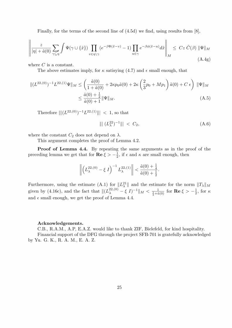
(A.4g)where C is a constant.

The above estimates imply, for κ satisying (4.7) and ε small enough, that

‖(L22,(0))−1L22,(1)Ψ‖M ≤(

a(0)1 + a(0)

+ 2κp0a(0) + 2κ

(23p0 + Mp1

)a(0) + C ε

)‖Ψ‖M

≤ a(0) + 12

a(0) + 1‖Ψ‖M . (A.5)

Therefore ‖|(L22,(0))−1L22,(1)‖| < 1, so that

‖| (L22λ )−1‖| < C2, (A.6)

where the constant C2 does not depend on λ.This argument completes the proof of Lemma 4.2.

Proof of Lemma 4.4. By repeating the same arguments as in the proof of thepreceding lemma we get that for Re ξ > − 1

2 , if ε and κ are small enough, then∥∥∥∥(L

22,(0)λ − ξ I

)−1

L22,(1)λ

∥∥∥∥ <a(0) + 1

4

a(0) + 12

.

Furthermore, using the estimate (A.1) for ‖L21λ ‖ and the estimate for the norm ‖Tλ‖M

given by (4.16c), and the fact that ‖(L22,(0)λ − ξ I)−1‖M < 1

12+a(0)

for Re ξ > − 12 , for κ

and ε small enough, we get the proof of Lemma 4.4.

Acknowledgements.C.B., R.A.M., A.P, E.A.Z. would like to thank ZIF, Bielefeld, for kind hospitality.Financial support of the DFG through the project SFB-701 is gratefully acknowledged

by Yu. G. K., R. A. M., E. A. Z.

25

REFERENCES

[1] Berezansky, Yu.M., Kondratiev, Yu.G., Kuna, T., Lytvynov, E.: On a spectralrepresentation for correlation measures in configuration space analysis, Methods Funct.Anal. Topology, 5, no. 4, 87-100 (1999).

[2] Bertini, L., Cancrini, N., Cesi, F.: The spectral gap for a Glauber-type dynamicsin a continuous gas, Ann. Inst. H. Poincare Probab. Statist., 38, 91108 (2002)

[3] Boldrighini C., Ignatyuk, I.A., Malyshev, V.A., Pellegrinotti A.: ”Random walk indynamic environment with mutual influence”, Stochastic Processes and their Applications,41, 157-177 (1992).

[4] Boldrighini, C., Minlos, R.A., Pellegrinotti, A.: ” Central limit theorem for therandom walk of one or two particles in a random environment”, Advances of Soviet Math-ematics, 20 : ”Probability Contributions to Statistical Mechanics”, R.L.Dobrushin, ed. ,21-75 (1994).

[5] Breiman, L.: ”Probability”, Classics in Applied Mathematics, 7. Soc. for Industrialand Appl. Mathematics, Philadephia, 1992.

[6] I.I. Gihman, A.V. Skorohod: The Theory of Stochastic Processes I. Grundlehrender mathematischen Wissenschaften, 210. Springer Verlag (1974).

[7] Yu. G. Kondratiev, R. A. Minlos: One-particle subspaces in the stochastic XYmodel, Journal of Stat. Physics, 87(3/4): 613-642 (1997).

[8] Kondratiev Yu. G., Minlos, R. A., Zhizhina, E. A.: ”One particle subspace of theGlauber Dynamics Generator for continuous Particle Systems”, Reviews in Math. Physics,16, n. 9, 1073-1114 (2004)

[9] Kondratiev, Yu.G., Kuna, T.: Harmonic analysis on conøguration spaces I. Generaltheory, Infin. Dimens. Anal. Quantum Probab. Relat. Top., 5, 201233 (2002)

[10]Yu. Kondratiev, T. Kuna, O. Kutoviy, On relations between a priori bounds formeasures on configuration spaces, Infinite Dimensional Analysis, Quantum Probability andRelated Topics, Vol.7 (2), p. 195-213, 2004.

[11] Kondratiev, Yu., Lytvynov, E.: Glauber dynamics of continuous particle systems,Ann. Inst. H.Poincare - PR 41, 685-702 (2005)

[12] Kondratiev, Yu., Roeckner, M, Lytvynov, E.: Equilibrium Glauber and Kawasakidynamics of continuous particle systems, BiBoS-Preprint (2005),

available at www.arxiv.org/math.PR/0503042[13] Malyshev, V.A., Minlos, R.A.: Linear infinite-particle operators, American Math-

ematical Society Publ., 1995[14] R. A. Minlos, Invariant subspaces of the stochastic Ising high-temperature dy-

namics, Markov Processes and Related Fields, 2 (2): 263-284, (1996).[15] Zeitouni, O., Random Walks in Random Environment. Ecole d’ Ete de Proba-

bilites de St. Flour, XXXI- 2001. Lecture Notes in Mathematics 1837. Springer Verlag,2004.

26