arX

iv:p

hysi

cs/0

6030

24v2

[ph

ysic

s.so

c-ph

] 1

8 Ja

n 20

10

Applying Free Random Variables

to Random Matrix Analysis of Financial Data

Part I: A Gaussian Case

Zdzis law Burda,1, ∗ Andrzej Jarosz,2, † Jerzy Jurkiewicz,1, ‡

Maciej A. Nowak,1, § Gabor Papp,3, ¶ and Ismail Zahed4, ∗∗

1Marian Smoluchowski Institute of Physics and Mark Kac Complex Systems Research Centre,Jagiellonian University, Reymonta 4, 30–059 Krakow, Poland

2Clico Ltd., Oleandry 2, 30–063 Krakow, Poland

3Institute for Physics, Eotvos University, 1518 Budapest, Hungary

4Department of Physics and Astronomy, SUNY Stony Brook, NY 11794, USA

(Dated: January 18, 2010)

We apply the concept of free random variables to doubly correlated (Gaussian) Wishart ran-dom matrix models, appearing for example in a multivariate analysis of financial time series, anddisplaying both inter–asset cross–covariances and temporal auto–covariances. We give a compre-hensive introduction to the rich financial reality behind such models. We explain in an elementaryway the main techniques of the free random variables calculus, with a view to promote them in thequantitative finance community. We apply our findings to tackle several financially relevant prob-lems, such as of an universe of assets displaying exponentially decaying temporal covariances, or theexponentially weighted moving average, both with an arbitrary structure of cross–covariances.

PACS numbers: 89.65.Gh (Economics; econophysics, financial markets, business and management), 02.50.Sk(Multivariate analysis), 02.60.Cb (Numerical simulation; solution of equations), 02.70.Uu (Applications ofMonte Carlo methods)

Keywords: random matrix theory, free random variables, risk management, noise, cross–correlations, auto–correlations, delay correlation matrix, RiskMetrics, EWMA, factor models

I. INTRODUCTION

A. Financial Cross–Correlations and Auto–Correlations From Gaussian Random Matrix Theory

1. Financial Correlations and Portfolio Optimization

Cross–correlations between assets traded on the markets play a critical role in the practice of modern–day financialinstitutions. For example, correlated moves of assets diminish a possibility of optimal diversification of investmentportfolios, and precise knowledge of these correlations is fundamental for optimal capital allocation: in the classicalMarkowitz mean–variance optimization theory [1], all the correlations must be perfectly known. Not only so, but afuture forecast of the correlations would be highly desirable. However, the information about cross–correlations andtheir temporal dynamics is typically inferred from historical data, stored in the memories of computers (usually inthe form of large matrices); the material decoded from past time series is inevitably marred by measurement noise,and it is a constant challenge to unravel signal from noise.

∗Electronic address: zdzislaw.burda@uj.edu.pl†Electronic address: andrzej.jarosz@clico.pl‡Electronic address: jerzy.jurkiewicz@uj.edu.pl§Electronic address: nowak@th.if.uj.edu.pl¶Electronic address: pg@ludens.elte.hu∗∗Electronic address: zahed@zahed.physics.sunysb.edu

2

One may argue that from the point of view of practical portfolio optimization, cross–correlations are only a“second–order effect,” since they represent fluctuations around a certain trend described by the average returns ofassets. Now it is well–known that the future returns are to a great extent impossible to determine from the historicalreturns (one would need to take a very long time series to account for volatilities, which would manifest a highlynon–stationary nature of the returns’ distribution), and are thus subject to individual assessment by managers. Wewill disregard this problem in the present analysis, and assume that investors have some expectations of the futurereturns, recalling at the same time that volatilities and cross–correlations should be much more stable in time (due tothe phenomenon of heteroscedasticity, i.e., time–dependence of volatility), hence allowing some level of predictabilityof their future values from historical data, once the measurement noise has been properly cleaned.

Another reservation (see for example [2]) may be that optimization leads to a solution for the portfolio weightsdependent on the covariance matrix in a stable way (in the sense that a small modification of the covariances leads toonly a small change in the portfolio composition and risk) only in simplest cases of linear constraints on the weights,while for non–linear constrains (present for example on futures markets) the problem becomes equivalent to findingthe energy minima of a spin glass system, and there is an exponentially large (in the number of assets) number of theselocal minima with an unstable (chaotic) dependence on the covariance matrix. Again, we will restrict our interestto portfolios with linear constraints on the weights, in which case the estimation noise of the covariance matrix isalready troublesome enough for special techniques of its elimination to be unavoidable.

Keeping these limitations in mind, we conclude that correlations between assets necessarily have to be includedin any risk analysis (portfolio optimization, option pricing). Even more importantly than investment purposes, oneshould investigate the covariance matrix out of a theoretical motivation, as its structure mirrors the interdependenciesof companies, as well as possesses a non–trivial temporal dynamics; both qualities crucial for better understanding ofthe underlying mechanisms governing the behavior of financial markets.

2. The Gaussian Approximation

The primary way to describe not only the volatilities but also cross–correlations in a universe of some N assets isthrough the two–point covariance function,

Cia,jb ≡ 〈RiaRjb〉 . (1)

We define ria ≡ logSi,a+1 − logSia ≈ (Si,a+1 − Sia)/Sia to be the return of an asset i = 1, . . . , N over a time intervala = 1, . . . , T , i.e., (approximately) the relative change of the asset’s price Sia between the moments of time aδt and(a + 1)δt, where δt is some elementary time step. (We disregard the known small “leverage effect” of anomalousskewness in the distribution of the returns: that the price increments, rather than the returns, behave as additiverandom variables.) Moreover, we denote Ria ≡ ria − 〈ria〉, which describe the fluctuations (with zero mean) of thereturns around the trend, and collect them into a rectangular N × T matrix R. The average 〈. . .〉 is understood astaken according to some probability distribution whose functional shape is stable over time, but whose parametersmay be time–dependent.

In this paper, we will employ a very simplified form of the two–point covariance function (1), namely with cross–covariances and auto–covariances factorized and non–random,

Cia,jb = CijAab (2)

(we will collect these coefficients into an N ×N cross–covariance matrix C and a T × T auto–covariance matrix A;both are taken symmetric and positive–definite). We will discover that the matrix of “temporal covariances” A is away to model two temporal effects: the (weak, short–memory) lagged correlations between the returns (see par. I C 1),as well as the (stronger, long–memory) lagged correlations between the volatilities (heteroscedasticity; par. I C 2). Onthe other hand, the matrix of cross–covariances (“spatial covariances,” using a more physical language) C models thehidden factors affecting the assets, thereby reflecting the structure of mutual dependencies of the market companies(par. I B 2). Importantly, both contributions are decoupled: the temporal dependence of the distribution of each assetis the same, and the structure of cross–correlations does not evolve in time; this is quite a crude approximation. Also,these are all fixed numbers; only in a subsequent work do we plan to explore another known way (a “random parametricdeformation”) of modeling temporal dependence of cross–covariances, that is, considering C to be a random matrixof a given probability distribution.

3

For our approach to be valid, both covariance matrices obviously must be finite. In fact, the current article dealsexclusively with the multivariate Gaussian distribution for the assets’ returns which displays the two–point covariances(2),

Pc.G.(R)DR =1

Nc.G.exp

−1

2

N∑

i,j=1

T∑

a,b=1

Ria

[C−1

]ijRjb

[A−1

]ba

DR =

=1

Nc.G.exp

(−1

2TrRTC−1RA−1

)DR, (3)

where the normalization constant Nc.G. = (2π)NT/2(DetC)T/2(DetA)N/2, and the integration measureDR ≡∏i,a dRia; the letters “c.G.” stand for “correlated Gaussian,” and the expectation map w.r.t. this dis-tribution will be denoted by 〈. . .〉c.G., while “T” denotes matrix transposition. In this case, the covariance matricesare finite, and moreover they are sufficient to fully characterize the dependencies of the Ria’s. However, in morerealistic situations, such as of financially relevant distributions having heavy power–law tails (with an exponent µ),the two–point covariance (in particular C) may not exist. The precise answer boils down to how these correlatednon–Gaussian distributions are defined (one can exploit a variety of methods: a linear model, a copula, a randomdeformation of some kind, a method based on freeness, on radial measures, etc.; see for example [3], sections 9.2,12.2.3, 12.2.4, and [4–6]), and we will postpone this discussion to forthcoming communications. Let us just mentionthat in some cases (such as a linear model of Levy stable variables, i.e., with µ < 2), C diverges, and anothermeasure of covariance should be devised (for example, the “tail covariance,” which quantifies the amplitude of thetail and asymmetry of the power–law product variable RiaRjb); even for µ > 2, when C exists, it is informative(especially from the point of view of portfolio optimization in the sense of minimizing value–at–risk) to use the tailcovariance, as it focuses on large negative events. However, we henceforth restrict our attention to only the correlatedGaussian distribution (3); on this simplest (and admittedly quite distant from reality) example we wish to advocateour approach, with a view to further generalize it to heavy–tailed distributions.

3. Free Random Variables

A decade ago, Bouchaud et al. and Stanley et al. [7, 8] suggested the use of Gaussian random matrix theory

(RMT) for addressing the issue of noise in financial correlation matrices. Since then, a number of results regardingthe quantification of noise in financial covariances have been derived using this tool [9–25], some of which maybe ofrelevance to risk management.

In this work, we would like to advertise the concepts of the free random variables (FRV) calculus as a powerfulalternative to standard random matrix theory, both for Gaussian and non–Gaussian noise. FRV may be thought of asan abstract non–commutative generalization of the classical (commutative) probability calculus, i.e., a mathematicalframework for dealing with random variables which do not commute, examples of which are random matrices. (Indeed,FRV was initiated by Voiculescu et al. and Speicher [26, 27] as a rather abstract approach to von Neumann algebras,but it has a concrete realization in the context of RMT, since large random matrices can be regarded as free randomvariables.) Its centerpiece is a mathematical construction of the notion of freeness, which is a non–commutativecounterpart of classical independence of random variables. As such, it allows for extending many classical resultsfounded upon the properties of independence into the non–commutative (random matrix) realm, particularly thealgorithms of addition and multiplication of random variables, or the ideas of stability, infinite divisibility, etc.

This introduces a new quality into RMT, which simplifies, both conceptually and technically, many random matrixcalculations, especially in the macroscopic limit (the bulk limit, i.e., random matrices of infinite size), which is ofmain interest in practical problems.

Several years ago, we suggested that FRV is very useful for addressing a much larger class of noise (Levy) in thecontext of financial covariance matrices in a way that is succinct and mostly algebraic [28–33]. These results havenow seen further applications to financial covariances [34–36] and macroeconomy [37]. Also, FRV has been alreadyapplied to a number of problems ranging from physics [38–40] to wireless telecommunication [41–44].

The primary aim of this publication is to advertise the framework of FRV to the audience of quantitative finance(QF) by re–deriving several known results obtained earlier through other (more laborious) methods of Gaussian RMT,as well as solving a few problems for the first time. This illustrates the fluency of the FRV calculus for noisy financial

4

covariances. In particular, we show how an FRV–based back–of–an–envelope calculation leads to a simple equation(61) for a function M ≡ Mc(z) (32) that generates all the moments (i.e., contains all the spectral information) of ahistorical estimator c (22) of the cross–covariance matrix C (2), in the presence of arbitrary “true” cross–covarianceand auto–covariance matrices C and A,

z = rMNA(rM)NC(M). (4)

Here the N ’s are certain functions (34), computable once C and A are known; and r ≡ N/T . (The unrealisticassumption about the Gaussian statistics of the financial assets’ returns will be relaxed only in subsequent papers,where generalizations of the current findings, among them (4), to the Levy FRV calculus will be presented; althoughrandomly sampled Levy matrices have one or even no finite spectral moments, FRV permits a straightforward analysisof the pertinent moments’ generating functions and thus the corresponding spectral distributions.)

This article is organized as follows:

• The remainder of this section I is devoted to discussing the motivations, meaning, and applicability of our resultsto the financial reality. Our working assumption of Gaussianity, its limitations and possible extensions, havealready been touched upon in par. I A 2. In subsec. I B, various commonly used models for the cross–covariancematrix C are presented, which may be used as an input for equation (4). This application is however limitedby the appearance of large eigenvalues in the spectrum of C, for which we give a brief justification; it calls for amore refined analysis than currently allowed by FRV. Subsec. I C deals with auto–covariances A. We show thatour method is well–poised to investigate the weak short–ranged auto–correlations observed on financial markets,triggered by non–zero transaction costs and the presence of bonds or interest rates, and included in modernrisk evaluation methodologies, but fails at this stage to handle more involved auto–covariances between differentassets, such as required for example to explain the Epps effect. We describe also the much more important long–memory auto–correlations between the random volatility of the returns (heteroscedasticity), and introduce somecorresponding weighting schemes, mainly the exponentially weighted moving average (EWMA). In subsec. I D,we define and discuss several standard historical estimators of the covariance matrices (Pearson, time–lagged,weighted).

• Section II is the centerpiece of this work. It commences in subsec. II A with a crash course in free randomvariables, with a particular focus on the addition and multiplication algorithms of free random matrices; thelatter constitutes the chief tool we exploit. It has a more operational flavor, designed to aid practical applicationsby the QF community rather than to delve into the mathematics behind the scenes. Subsec. II B gives aforetaste of the power of the FRV approach by re–computing in an algebraic way the famous Marcenko–Pasturdistribution. The salient part comes in subsec. II C, where equation (4), along with its variations, is derived andpresented.

• Section III contains two examples of how the main formula (4) can be used to tackle financially relevant problems.Namely, we find equations for the moments’ generating functions M of the standard and time–delayed historicalestimators in the presence of exponentially decaying temporal auto–covariances and arbitrary cross–covariances(subsec. III A), as well as of the EWMA with arbitrary cross–covariances (subsec. III B). In the simplest caseof no underlying cross–covariances, we reinforce our analytical findings with numerical simulations.

• The article terminates with short conclusions and some possible prospects for the future in section IV (more areactually given inside the body of the article), as well as a list of references.

B. Modeling Cross–Correlations

1. Principal Component Analysis

In this subsection, we consider a fixed moment in time, a, and investigate the cross–correlations between theassets; assuming the decoupling (2), their structure C does not depend on time. Being symmetric and positive–definite, C can be diagonalized, Cvk = λkvk, with N real and positive eigenvalues (they can be ordered decreasing,λ1 ≥ . . . ≥ λN > 0), and N orthogonal and normalized eigenvectors. This diagonalization is called a “principal com-ponent analysis” (PCA), because the knowledge of the eigenvectors of C allows to linearly transform the N correlated

5

entities Ria into N uncorrelated ones (referred to as “principal components” or “explicative factors”) eka, whosevariances are given by the eigenvalues of C,

eka ≡N∑

i=1

vk,iRia, or conversely, Ria =N∑

k=1

vk,ieka, where 〈ekaela〉 = λkδkl. (5)

In other words, the PCA unravels the uncorrelated (not necessarily independent) factors affecting the collection ofassets, and orders them w.r.t. their decreasing volatility. Since a factor is a certain mix of the assets (i.e., a portfolio),we can restate it yet differently by that the PCA derives a set of uncorrelated investment portfolios, and orders themw.r.t. their decreasing risk.

2. Factor Models

There have been put forth models of the structure of the covariance matrix (see for example [3], section 9.3). Theyare to reflect the structure of the spectra of its estimators built from historical financial data (see subsec. I D), whichtypically consist of one very large eigenvalue, several smaller but still large ones, and a sea of small eigenvalues, whosedistribution can be very accurately fitted with the Marcenko–Pastur distribution [45] of the eigenvalues of a purelyrandom matrix belonging to the (uncorrelated) Wishart ensemble [46]. As we discuss in more detail in subsec. I D,an estimator of the covariance matrix will necessarily contain a lot of measurement noise, and these decade–oldresults [7, 8], pioneering the use of random matrix theory in financial applications, suggest that actually most of thespectrum is purely random, with the exception of the largest eigenvalues “leaking out” of the bulk Marcenko–Pasturdistribution, which do carry some information about the true correlations between the assets. For example, theappearance of one very large eigenvalue λ1 (c.a. 25 times greater than the upper bound of the noise distribution forthe S&P500 data in [7]) has the following meaning: Since e1 fluctuates with such a dominating volatility, the PCA (5)can be approximated as Ri ≈ v1,ie1 (we skip the index a in this paragraph), which means that the dynamics of all theassets is governed practically by just one factor. The corresponding eigenvector has roughly all the components equal,which thus represents a portfolio with approximately the same allocation in all the assets, i.e., with no diversification;this portfolio will therefore be strongly correlated with the market index, and is thus called the “market factor.” Itspresence in the empirical spectrum may be understood for instance in terms of the herding phenomenon (a collectivebehavior of the investors). Similarly, other large eigenvalues seen in the spectra of historical covariance matricescan be attributed to the clustering of individual companies into industrial sectors (constructed by investigating therelevant eigenvectors), within which the correlations are strong.

Consequently, one may attempt to model the matrix C in order to reproduce such empirical observations; thisprogram goes under a name of “factor component analysis” (FCA), since it aims at describing a large number ofcross–correlations between assets in terms of their correlations with a much smaller number of factors. To begin with,one considers a “one–factor model” (“market model”) [47], where it is assumed that each return Ri is impacted bythe market return φ0 with some strength βi (named the “market beta” of this asset), and besides that there is nocorrelation between assets; namely, it approximates Ri = βiφ0 + ei, where φ0 and the ei’s (called the “idiosyncraticnoise”; their presence implies that the underlying factors cannot be directly observed as they are marred by randomerrors) are uncorrelated and have the volatilities Σ and σi respectively; the model is described by (2N +1) parameters.The covariance matrix thus reads

Cij = Σ2βiβj + σ2i δij . (6)

It can be easily diagonalized under an additional simplification that all the σi’s are equal to some σ0, in which casethere is one large (∝ N ; we generically assume N to be large, see (18)) eigenvalue λ1 = Σ2β2 + σ2

0 , correspondingto v1 ∝ β (the “market”), and an (N − 1)–degenerate eigenvalue σ2

0 (if the σi’s are unequal but of comparable size,there is a large market eigenvalue and a sea of (N − 1) small ones).

A more refined “multi–factor model” [18, 48, 49], describing increased correlations within industrial sectors, as-sumes that the idiosyncratic (non–market) parts ei are exposed to K hidden factors φα, namely ei =

∑Kα=1 βiαφα + ǫi,

where all the factors and the new idiosyncratic terms are uncorrelated and have the volatilities Σα and σi respectively.In this case,

Cij = Σ2βiβj +K∑

α=1

Σ2αβiαβjα + σ2

i δij . (7)

6

To further (quite drastically) simplify this model, we may consider that each asset i is exposed to only one factorα, with Nα assets belonging to sector α (

∑Kα=1 Nα = N), which translates into βiα = β(α′ i)α = δα′αβ

(α′)

i, where the

index i is split into a double–index (α′ i), with α′ enumerating sectors and i assets within sector α′. Also we considerthe exposures to the market negligible as compared to the industrial ones (βi = 0), and the idiosyncratic volatilitiesdepending only on the sector, σi = σ(αi) = σα. Then C acquires a block–diagonal form, which is easily diagonalizedto give K “large” eigenvalues λα = Σ2

αβ(α)2 + σ2

α plus K “small” (Nα − 1)–degenerate eigenvalues σ2α. It mirrors

more properly the existence of several large eigenvalues. The form of the covariance matrix can also be specified alonganalogous lines in more complex ways, such as in the “hierarchically nested factor model” (HNFM) [50].

Any such model can be used as a non–statistical input for equation (4). In this way, the number of parametersto be estimated (for which the Pearson’s chi–square method may be used) is typically greatly reduced, however onthe cost of a specification error. Another problem with the above models is that their generic feature is the existenceof isolated “large” eigenvalues (i.e., proportional to the size of the portfolio N and with a microscopic degeneracy,typically singlets), while the FRV tools seem not adequate enough to tackle such situations yet, being restricted tothe bulk of the distribution, and thus other methods should be employed (see for example [51]). This is why in thisarticle we refrain from using our main formula (4) for any nontrivial cross–covariance matrix C, focusing rather ontemporal covariances; this obstacle should certainly be dealt with.

C. Modeling Auto–Correlations

1. Lagged Correlations Between the Returns

Let us now discuss which empirical facts concerning temporal correlations can be modeled (and how) withinour very simplified framework (2). First, it is well–known that the returns are weakly auto–correlated on shorttime scales: the delayed correlation function (see (23) for its definition) is significantly different from zero (and, forexample, negative for stocks, but positive for stock indices) for the time lags less than c.a. 30 minutes for liquid andfree–floating assets (longer on less liquid markets; this decay lag also decreases with time), see [3], sections 6.2, 13.1.3.The simplest and most natural model for such a behavior, for a single asset i, is an exponential decay,

〈RiaRib〉〈R2

ia〉= e−|b−a|/τ , (8)

with the characteristic time τ (given here in the units of δt) of the order of several minutes.

Let us emphasize that we are talking about correlation functions here, i.e., normalized by the variance. Thevariance have completely different, stronger, long–memory temporal dynamics (heteroscedasticity; see par. I C 2),allowing forecasts of future volatilities from past data. From this point of view, heteroscedasticity is a “first–ordercorrection” to an iid of the returns, while the auto–correlation of the returns (such as (8)) is a “second–order effect.”Consequently, any long–term forecast of the mean returns seems impossible, and we will focus on forecasting thevolatility, used then to assess the short–term risk of a portfolio. Anyway, on short time horizons (such as one businessday), the mean return is negligible (say, a small fraction of a percent for stocks) as compared to its volatility (a fewpercent).

These weak auto–correlations should not however be disregarded. Actually, they may persist on longer timescales, such as days, but to reveal that, one would need to consider much longer (decades) historical time series inorder to decrease the estimation noise; there might even be auto–correlations over time spans of a few years, reflectingthe existence of economic cycles. If detectable auto–correlations were present for longer lags, they could be used todevise a profitable trading strategy until arbitrage would remove them; this is the efficient market hypothesis. Buteven such weak and short–memory auto–correlations allow in principle to attain large profits in high–frequency (HF)trading; however, when transaction costs are taken into account, these profits are precisely discounted, and this isone reason that a non–zero decay lag is allowed without contradicting the efficiency of the markets. Another reasonis the existence of riskless assets (bonds), which implies that stocks should gain on average the riskless rate of returnand additionally a risk premium; moreover, short–term interest rates are not free–floating (they are set by the centralbanks and are usually quite predictable). For these reasons, the auto–correlations, albeit weak, begin to be includedinto new risk evaluation methodologies, such as RiskMetrics 2006 [52], which even attempts to predict the meanreturns (and thus risks) for long–time horizons, up to one year. Our approximation (2) should be able to handle

7

effects like (8), and in subsec. III A we indeed show an application of equation (4) to a model with an exponentiallydecaying auto–covariance matrix A.

However, this phenomenon of non–zero lagged correlations should be extended from a single asset to multiple

variables: the returns of different assets are correlated between different time moments. This is crucial, for example,for gaining insight into the dynamics of the cross–correlations as we progress from the HF time scale to longer timescales. The strength of the equal–time cross–correlation between assets i 6= j was long ago observed to grow withincreasing δt (when moving from higher to lower sampling frequencies, the equal–time inter–asset correlations rapidlyrise on the scales of several minutes, to saturate on the scales of days), which is called the “Epps effect” [53]. Not onlythis, but the entire structure of cross–correlations (depicted through the maximum spanning tree of the market [54])evolves as an embryo which expands and differentiates as δt enlarges. This change of strength and structure of cross–correlations is, for instance, critical for the possibility of increasing the sampling frequency in order to obtain longertime series, and as a result, less noisy historical estimators (see par. I D 1): one cannot probe too deep into the HFregime (far from the saturation level of the Epps curve) since then the entire tree of cross–correlations looks totallydifferent. This is yet another reason for developing noise–cleaning procedures, such as the one advocated in this paper.In order to explain the Epps effect, a causal relation must be present between the time evolution of the return of asseti at a certain time and the returns of all the other assets j 6= i at all the previous moments. For example, in [55, 56],the equal–time cross–correlations are expressed through delayed cross–correlations over shorter time scales, and thelatter are modeled by a direct analog of the exponential decay (8), just with separate i and j,

〈RiaRjb〉〈RiaRja〉

= e−|b−a|/τ ; (9)

this eventually proves to provide an analytical shape of the Epps curve which is remarkably close to the experimentalone. Another, more complex model of linear causal influence is presented in [35],

ri(t) = ei(t) +

N∑

j=1

∫ +∞

−∞dt′Kij (t− t′) rj (t′) , (10)

where ei(t) is an idiosyncratic part, and Kij(t− t′) is called the “influence kernel.” However, these models cannotbe captured by our current simple framework (2), (4), and it certainly is an interesting challenge to extend the FRVapproach so that it could be helpful in an analytical treatment of such more involved correlations, responsible amongother things for the Epps effect.

2. Heteroscedasticity

A well–established “stylized fact” observed in all financial time series is that the (say, daily) volatility of an asset’sreturn depends on time, displaying a “long memory,” namely that periods of high or low volatility tend to persistover time; this property is known as “heteroscedasticity,” “volatility clustering,” or “intermittence” (by analogy withturbulent flows of fluids, where a similar phenomenon of persistent intertwined periods of laminar and turbulentbehavior occurs). A standard approach to describe mathematically this experimental fact is to suppose that not onlyis the demeaned and normalized return ǫia (the “residual”) a random variable, but so is the volatility σia,

Ria = σiaǫia. (11)

These two sources of randomness are to a great extent inseparable, and it becomes a matter of choice how to modelthem in order to jointly arrive at results which comply with empirical data; for example, a Student distribution forthe return can originate from an inverse–gamma randomness of the variance superimposed on a Gaussian iid of theresiduals. Such a very general depiction (11), with the ǫia’s assumed to be iid with zero mean and unit volatility andthe σia’s some random variables possibly correlated with each other and also with the residuals, is named a “stochasticvolatility model”; see [3], section 7.

Indeed, the volatilities at different time moments are correlated. These lagged correlations are not strong (severalpercent, depending on the volatility proxy used and the time lag chosen), but stretch over much longer periods thanthe lagged correlations of the residuals, discussed in par. I C 1: their slow decay (long–memory) can be modeled wellby a power law, 1/|b− a|ν , where a fit of the exponent ν typically lies in the range 0.2÷0.4 (depending on the domainof the time lags considered). In other words, the temporal dynamics of the volatility is a multi–scale phenomenon.

8

Moreover, the probability distribution of (an estimator, such as the “high–frequency proxy,” being the daily averageof HF returns, of) the volatility may be approximated by an inverse–gamma or a log–normal shape.

A basic idea, founded upon the presence of the long–memory lagged volatility correlations, is to regard thevolatility as undergoing a certain stochastic process. A convenient feature of this approach is its consistency: thevolatility process should be constructed from historical time series (in particular, it should reflect a power–law–likedecay of the lagged correlations), and thus obtained parameters are then used to make forecasts (through evaluatingconditional averages) for the value of the volatility over some future time horizon ∆t. In other words, even long–time horizons become available for meaningful risk assessment; although of course for long ∆t the deficiency of pastdata excludes a possibility of backtesting of these forecasts. There exists a plethora of propositions for volatilityprocesses. One selecting requirement is actually computational accessibility of forecasting, which practically reducesthe possible choices to quadratic processes only, i.e., where the variance depends linearly on the past squared returns,see below. This still yields a very broad class of processes, falling under the name of “auto–regressive conditionalheteroscedasticity” (ARCH).

A standard textbook example, reflecting to some extent the behavior of financial time series, is the GARCH(1, 1)model [57–59],

σ2a = w∞σ2

mean + (1 − w∞)σ2hist.,a, σ2

hist.,a = ασ2hist.,a−1 + (1 − α)R2

a−1 (12)

(the asset index i is skipped here and in the remainder of this paragraph). In the above, σ2mean is the unconditional

mean variance, representing the average long–run value of the variance, and σ2hist.,a is a “historical (auto–regressive)

variance,” depending linearly on both itself and the realized squared return at the preceding time moment (the dailyfrequency is typically used). The constant w∞ is a “coupling,” while α ∈ [0, 1] may be thought of as measuring theresponsiveness of the variance to the recent realized variance R2

a−1: α close to 1 means that the variance respondsquite slowly to the news. (We may also write (12) differently, σ2

a = σ2mean + g1(σ2

a−1 − σ2mean) + g2(R2

a−1 − σ2a−1),

where g1 ≡ 1 − w∞(1 − α) and g2 ≡ (1 − w∞)(1 − α), in order to see that the process tries to revert the volatilityto its mean value with strength g1, and also incorporates a feedback of the difference between the realized squaredreturn R2

a−1 and its mean value σ2a−1 on the next–day value of the variance, to which effect a magnitude g2 is given.)

There are two problems with this traditional model. First, it is an “affine” (“mean–reverting”) process, i.e.,containing the additive term w∞σ2

mean, whose meaning is that in the long run, the average volatility will convergeto the value σmean regardless of the initial conditions. To every affine process, there exists a corresponding “linear”(“integrated”) process, which simply removes the unconditional expectation by setting w∞ = 0, in which case thelong–term mean volatility depends on the initial conditions or may even not converge; for example, (12) will yield amodel called I–GARCH(1). Only the integrated processes can be successfully harnessed for risk forecasts. The reasonis that an integrated model is described by two parameters less than its mean–reverting counterpart (namely, w∞ andσmean), and the latter of these is strongly time series dependent; in other words, for a portfolio of N assets, an affinemodel would contribute a large number N of mean unconditional volatilities for estimation, which would produce ahuge measurement error. In I–GARCH(1), on the other hand, there is only one parameter α accounting for all theassets that requires estimation.

More importantly, both GARCH(1, 1) and I–GARCH(1) (let us henceforth focus on the integrated versions only)fail to reproduce the observed power–law decay of the time–lagged volatility correlations, leading instead (the cal-culation is doable analytically) to an exponential decay, with the characteristic time (in the units of δt = one day)τ = −1/ logα,

⟨σ2aσ

2b

⟩−⟨σ2a

⟩ ⟨σ2b

⟩∝ e−|b−a|/τ . (13)

This may be seen in yet another way by unwinding the second part of (12), thus casting the variance as a linearfunction of the past squared returns,

σ2a =

1 − α

1 − αT

T∑

b=1

αb−1R2a−b, (14)

where a necessary cutoff T is introduced. The “weights” with which the past squared returns impact the today’svariance, scale exponentially as we move backward in time (∝ αb−1); this short–memory scheme is called the “ex-ponentially weighted moving average” (EWMA), see for example [60], chapter 21, and [61, 62]. Despite this evidentshortcoming, the I–GARCH(1) (EWMA) volatility process has very successfully transpired into the every–day prac-tice of many financial institution by being woven into the commonly accepted risk evaluation methodology, RiskMet-rics 1994 [63, 64]. It was probably due to its simplicity, as it is described by just one parameter α shared by a wide

9

range of securities (its value found to yield forecasts which come closest to the realized variance is α = 0.94, i.e.,τ = 16.2 business days), which is critical since the methodology is to be applied to a great many time series; andmoreover, it utilizes only the one previous–day observation to update the volatility (so little data needs to be stored).

Let us briefly mention that the framework of integrated models can be extended to accommodate for the long–memory correlations [65, 66], culminating in the fresh RiskMetrics 2006 [52]. Such processes are still quadratic,

σ2a =

T∑

b=1

wbR2a−b, (15)

where the weights wb are positive and obey the “sum rule,”∑T

b=1 wb = 1. For example, RiskMetrics 2006 argues thata logarithmic decay consistently proves to be an even better fit to financial data than a power law,

wb ∝ 1 − log(bδt)

log τ0, (16)

where again one parameter τ0 ∼ 3 ÷ 6 years is enough to capture the long memory of diverse time series. (Forsmall time lags, the power–law and log–decay are very similar, with their parameters related approximately throughν = 1/ log(τ0/δt). But for longer lags, say beyond one month, the logarithmic fit visibly stands out in quality.)

Our FRV technique is not yet suited for handling ARCH models like discussed above. However, the FRV calculusdoes bring considerable simplification into working with historical estimators of cross–covariance matrices whichincorporate weighting schemes (15), such as the EWMA (14) or log–decay (16). They will be defined in par. I D 3,and the case of the EWMA (with all its defects and advantages just highlighted) will be addressed in subsec. III B.

D. Historical Estimation of the Covariance Matrices

1. Estimators of Equal–Time Cross–Covariances

A fundamental problem is how to reliably estimate the covariance matrices from the available historical data [67,68]. One obstacle lies in the finiteness of the time series, due to which any estimator will contain an amount ofmeasurement noise. Let us focus for definiteness on estimating C: since there are N(N + 1)/2 independent entriesin C, and we have at our disposal N time series of length T each (collected in a historical realization R; we will notdistinguish in notation between random variables and their actual realizations), thus the level of the estimation noisemay be quantified by the “rectangularity ratio”

r ≡ N

T. (17)

If r → 0 (thanks to T → ∞ with fixed N , which is a limit commonly used in statistics), any empirical covariancematrix should approach the exact one (i.e., it should be asymptotically unbiased). However, r close to zero is usuallyfar from financial reality, in which both T and N are large and of comparable size; for example, one may have dailydata from several years (each of about 260 business days) and may want to consider a major bank’s portfolio consistingof several hundred of even thousands of assets; hence, the relevant regime is rather the “thermodynamical limit,”

N → ∞, T → ∞, such that r = fixed. (18)

Therefore, any estimator will be (seriously, for realistic values of r) dressed with the measurement noise, and it is ofparamount importance (from the point of view of risk management, for example) to devise methods which detect inthe noised estimators information about the true covariances (“cleaning” of the measurement errors); these de–noisedestimators can then serve for practical purposes (such as evaluating the risk of a portfolio). (Remark that (18) is alsoprecisely the limit in which the standard techniques of random matrix theory are applicable to the random matrix R;to be used below.)

The matrices C and A can be estimated from the past time series R by, for example,

c ≡ 1

TRRT, a ≡ 1

NRTR, (19)

10

which may be called their Pearson estimators (the usual prefactors 1/(T − 1) and 1/(N − 1) are replaced in the aboveby 1/T and 1/N , respectively, since we can approximately disregard the average value of the returns in comparisonwith their volatilities over the considered time horizons; see par. I C 1). For any probability distribution of the returnssuch that (2) holds with finite C and A, it is easily checked that the Pearson estimators (19) are, up to rescalings,unbiased,

〈c〉 = MA,1C, 〈a〉 = MC,1A, (20)

where MC,1 ≡ 1N TrC and MA,1 ≡ 1

T TrA are the first moments of the matrices C and A, see below (30). For thecorrelated Gaussian distribution (3), the Pearson estimators are proportional to the respective maximum likelihoodestimators.

It is clear that cij = 1T

∑Ta=1 RiaRja represents the equal–time covariance between assets i and j averaged over

time; similarly, aab = 1N

∑Ni=1 RiaRib shows how the measurements at moments a and b are correlated on average for

all the assets. These two seemingly very different quantities are in fact very closely related: since RRT and RTR havethe same non–zero eigenvalues (the larger one has additionally |T −N | zero modes), thus c and a have also identicalnon–zero eigenvalues up to the factor of r (the latter are 1/r times the former). In other words, the informationcontent of c and a is equivalent, describing the structure of equal–time correlations between the assets; we will thusabandon a henceforth. We will state this point in more quantitative terms (47) in par. II B 2.

As is well–known, it is possible to describe the N ×T correlated Gaussian random variables R in terms of N ×Tuncorrelated Gaussian variables R; this is achieved through the change R =

√CR

√A (the covariance matrices are

symmetric and positive–definite, therefore their square roots exist), which transforms the correlated Gaussian measure(3) into the uncorrelated one,

PG.(R)DR =1

NG.exp

(−1

2TrRTR

)DR =

1

NG.exp

(−1

2

N∑

i=1

T∑

a=1

R2ia

)DR, (21)

with NG. = (2π)NT/2, and 〈. . .〉G. denoting the expectation map w.r.t. this probability distribution. Correspondingly,the estimator c becomes in the new language more involved,

c =1

T

√CRART

√C. (22)

With R a random matrix drawn from the distribution (21), the estimator c (22) is called a “doubly correlatedWishart” random matrix.

2. Estimators of Time–Delayed Cross–Covariances

It is of course desirable to find an estimator of temporal correlations, i.e., correlations between two assets at twodifferent moments in time. It is commonly done through the “lagged covariance matrix estimator,” which representsnon–equal–time (with a time lag d, an integer divisor of the total time series length T , t ≡ T/d = 2, 3, . . .) covariancebetween assets i and j averaged over time,

c(d)ij ≡ 1

T

T−d∑

a=1

RiaRj,a+d, i.e., c(d) =1

TRD(d)RT, where D

(d)ab ≡ δa+d,b. (23)

This matrix is non–symmetric, and it will be very interesting to develop a method to deal with it (see [69] for a solution,based on the circular symmetry of the problem and the Gaussian approximation, in the simplest case of C = 1N andA = 1T ; here 1K denotes the unit K × K matrix). In the present paper, however, we will not attempt this morechallenging task, leaving it for future work, but only resort to the simplification [70] of considering a symmetrizedversion of (23),

csym.(d) ≡ 1

TRDsym.(d)RT, where D

sym.(d)ab ≡ 1

2(δa+d,b + δa−d,b) , (24)

which becomes symmetric, and therefore tractable within our present approach, but still carries some informationabout delayed correlations between assets. In terms of the uncorrelated Gaussian variables (21) it reads

csym.(d) =1

T

√CR

√ADsym.(d)

√ART

√C. (25)

11

This is also a doubly correlated Wishart random matrix, akin to c, albeit with a modified underlying auto–covariancematrix, A →

√ADsym.(d)

√A.

3. Estimators with Weighting Schemes

The standard Pearson estimator cij of the cross–covariance between assets i and j (19) is defined as the averageof the realized cross–covariances RiaRja over the past time moments a. In this way, all these past values of therealized cross–covariance have an equal impact on the estimator of the today’s cross–covariance. However, whendiscussing an analogous problem for the estimates of the variance in par. I C 2, we discovered that the phenomenon ofheteroscedasticity, modeled by some quadratic ARCH stochastic process (15), implies the presence in financial timeseries of a long memory, described by the weights wa (of a power–law or logarithmic decay, but frequently used aswell is an exponential decay, i.e., the EWMA). In other words, the older the realized variance R2

ia, the more obsoleteit is, i.e., the more suppressed its contribution to the estimator of the today’s variance is, as given by the weight wa.(Here we will adopt a convention that in our time series, enumerated by a = 1, . . . , T , the most recent observation isa = 1, and moving backward in time as a increases.) Now, it is a common practice to set up the updating schemes forthe cross–covariances by simply mimicking the schemes for the variances; see [60], compare also the discussion in [66].Therefore, we will consider the following general class of “weighted estimators” of the cross–covariances,

cweightij ≡

T∑

a=1

waRiaRja, i.e., cweight =1

TRWRT, where W ≡ Tdiag (w1, . . . , wT ) . (26)

Again, it is convenient to convert the correlated Gaussian random variables R into the uncorrelated ones R, whichleads to an expression analogous to (25),

cweight =1

T

√CR

√AW

√ART

√C, (27)

which is the doubly correlated Wishart ensemble with the underlying covariance matrices C and√AW

√A. In this

way, also the weighted estimators have been grasped by our general framework.

II. FREE RANDOM VARIABLES: A PROMISING APPROACH TO THE ESTIMATION OF

COVARIANCE MATRICES

A. The Free Random Variables Calculus in a Nut–Shell

1. The Basic Notions of Random Matrix Theory

When studying (see for example [71, 72]) a real symmetric (or complex Hermitian) K × K random matrix H,drawn from some probability distribution P (H), perhaps a most natural question is about the probability distributionof its (real) eigenvalues λ1, . . . , λK , which is quantified by the “mean spectral density,”

ρH(λ) ≡ 1

K

K∑

i=1

〈δ (λ− λi)〉 =1

K〈Tr (λ1K −H)〉 , (28)

where δ(λ) is the real Dirac delta function, the expectation map 〈. . .〉 is performed w.r.t. P (H), and we recall that1K denotes the unit K ×K matrix.

This statistical information about the spectrum is equivalently encoded in the “Green’s function” (also called“resolvent,” “Cauchy transform” or “Stieltjes transform”), which is a complex function of a complex variable z,

GH(z) ≡ 1

K

K∑

i=1

⟨1

z − λi

⟩=

1

K

⟨Tr

1

z1K −H

⟩=

∫

cuts

dλρH(λ)1

z − λ. (29)

12

For finite K, this is a meromorphic function, with the poles at the λi’s on the real axis. On the other hand, inthe usually considered limit of an infinitely large random matrix (K → ∞), the mean eigenvalues tend to mergeinto continuous intervals (“cuts”; they can be infinite or finite, connected or not), and the Green’s function becomesholomorphic everywhere on the complex plane except the cuts on the real line. As such, it can typically be expandedinto a power series around z → ∞,

GH(z) =∑

n≥0

MH,n

zn+1, MH,n ≡ 1

K〈TrHn〉 =

∫

cuts

dλρH(λ)λn, (30)

where the coefficients are called the “moments” of H. In particular, in the strict limit z → ∞, it must obey

GH(z) → 1

z, for z → ∞. (31)

The above expansion (30) suggests working with an alternative object to the Green’s function, namely the “generatingfunction of the moments” (or the “M–transform”), simply related to the former,

MH(z) ≡ zGH(z) − 1 =∑

n≥1

MH,n

zn. (32)

We will be using both, depending on convenience, but chiefly (32). However, we stress that even if the moments donot exist, and thus the expansions (30), (32) are not valid, the knowledge of the analytical structure of the Green’sfunction (29) is sufficient to extract the statistical spectral properties of the random matrix.

Namely, once the Green’s function has been derived, the corresponding mean spectral density is found by usingthe Sokhotsky’s formula, limǫ→0+ 1/(λ + iǫ) = pv(1/λ) − iπδ(λ), which yields

ρH(λ) = − 1

πlimǫ→0+

ImGH(λ + iǫ). (33)

In other words, the density is inferred from the behavior of the Green’s function in the imaginary vicinity of theeigenvalues’ cuts on the real axis.

Finally, let us introduce the functional inverses of the Green’s function and the moments’ generating function,

GH (BH(z)) = BH (GH(z)) = z, MH (NH(z)) = NH (MH(z)) = z. (34)

The former has somewhat fancifully been named [73] the “Blue’s function” (known also under other names in liter-ature), while the latter will more conservatively be called the “N–transform.” These two functions are fundamentalobjects within the FRV approach, see below. Additionally, the Blue’s function can be expanded into a power seriesaround z = 0: it must start from a singular term 1/z due to (31) plus a regular expansion,

BH(z) =1

z+∑

n≥0

KH,n+1zn, (35)

where the coefficients, for the reason explained below, are referred to as “free cumulants.” (Let us mention thatthere is another commonly exploited object equivalent to the Blue’s function, which subtracts the singular term fromthe above expansion, and is named the “R–transform,” RH(z) ≡ BH(z) − 1/z. We will however adhere to using theBlue’s function.)

2. The Basic Notions of the Free Random Variables Calculus

Let us now detail the key features of the so–called “free random variables” (FRV) calculus, presented parallel tothe corresponding notions in the standard probability calculus.

An important problem in classical probability [74] is to find the probability density function (PDF) ofthe sum of two random variables, x1 + x2, provided they are independent, and we are given their separatePDFs, Px1 and Px2 . This is readily solved by applying the Newton’s formula to the moments of the sum,

13

Mx1+x2,n = 〈(x1 + x2)n〉 =∑n

k=0

(nk

)Mx1,kMx2,n−k. The moments are conveniently encoded in terms of the “charac-

teristic function,” which is a Fourier transform of the PDF,

gx(z) ≡∑

n≥0

Mx,n

n!zn = 〈ezx〉. (36)

(Here z must be a purely imaginary number on account of convergence of the sum over n, but we will not explicitlyprint this for the sake of future reference.) The above addition rule for the moments can be re–stated as that thecharacteristic function is multiplicative under the addition of independent random variables. In other words, itslogarithm,

rx(z) ≡ log gx(z), (37)

is additive,

rx1+x2(z) = rx1(z) + rx2(z), for independent x1, x2. (38)

This may be named the “classical addition law”; it shows that the addition problem for classical independent randomvariables is solved by (i) forming the Fourier transforms of the PDFs Px1 and Px2 , i.e., the characteristic functions, (ii)taking their logarithms, (iii) using the fact that the logarithms of the characteristic functions are additive, (iv) removingthe logarithm, which yields the characteristic function, and so also the moments and the PDF, of the sum x1 + x2.(The logarithm of the characteristic function can be expanded in a power series around z = 0, rx(z) =

∑n≥1 kx,nz

n.Its coefficients are called the “cumulants,” and are obviously additive, kx1+x2,n = kx1,n + kx2,n, upon the addition oftwo independent random variables.)

It is very far from trivial how to extend these steps into the case of random matrices, i.e., from the commutativeto non–commutative level, and it is the FRV theory of Voiculescu et al. and Speicher [26, 27] that develops a preciseanswer to this question. First of all, FRV puts forth a powerful concept of “freeness,” which is a non–commutativeanalog of independence. We will not delve too deep into explaining its construction, but let us show how it differsfrom classical independence. Namely, in classical probability, x1 and x2 are independent if their demeaned versions,X1,2 ≡ x1,2 − 〈x1,2〉, obey 〈X1X2〉 = 0. In non–commutative probability, the m non–commutative random variables(random matrices) x1, . . . ,xm are called “free” if their demeaned versions Xj ≡ xj − 〈xj〉 satisfy

〈p1 (Xj1 ) . . . pn (Xjn)〉 = 0, (39)

for all positive integers n, all polynomials p1, . . . , pn, and all indices j1, . . . , jn = 1, . . . ,m such that j1 6= j2 6= . . . 6= jn.For example, if x1 and x2 are free, there will be 〈x2

1x22〉 = 〈x2

1〉〈x22〉, i.e., just like for independent classical variables,

but also 〈x1x2x1x2〉 = 〈x21〉〈x2〉2 + 〈x1〉2〈x2

2〉 − 〈x1〉2〈x2〉2, much differently than in the commutative situation. Inother words, the mixed moments of free non–commutative random variables generally do not factorize into separatemoments, as it is the case for independence. Freeness is therefore a much more involved property. To give a practicalsummary, let us state that random matrices drawn from factorized distributions exhibit (asymptotically, i.e., whentheir sizes tend to infinity) freeness. (Borrowing a picture from physics, we may say that freeness is equivalent toplanarity in the limit of a large number of colors in field theory [75, 76].)

Freeness is a relevant idea because the problem of adding two free non–commutative random variables, x1 + x2,can be solved in a way analogous to its classical counterpart. Without any proofs (which are not very complicatedbut lengthy), we will just describe the resulting procedure:

Step 1: The moments of the free random matrices, x1 and x2, are conveniently encoded in the Green’s functionsGx1(z) and Gx2(z) (29), (30).

Step 2: The Green’s functions are inverted functionally to obtain the respective Blue’s functions Bx1(z) and Bx2(z)(34).

Step 3: The Blue’s functions obey the “non–commutative addition law,”

Bx1+x2(z) = Bx1(z) + Bx2(z) − 1

z, for free x1, x2. (40)

(Equivalently, this means that the R–transforms are additive, Rx1+x2(z) = Rx1(z) + Rx2(z). Trivially, the freecumulants (35) are additive as well, Kx1+x2,n = Kx1,n + Kx2,n. Let us also mention, for the readers familiarwith the Feynman diagrammatic techniques, that the additivity of the R–transform can be explained in termsof the additivity of the self–energy.)

14

Step 4: Invert functionally Bx1+x2(z) to find the Green’s function of the sum, Gx1+x2(z), and subsequently, its meanspectral density ρx1+x2(λ) through the Sokhotsky formula (33).

We recognize that it parallels the classical construction: the Green’s function is an analog of the characteristicfunction (36), functional inversion and forming the R–transform replaced taking the logarithm (37), and the additionlaw is a direct generalization of the classical one (38). The correspondence between the classical probability calculusand matrix probability calculus (FRV) is thus summarized in the following chart:

PDF ↔ spectral density↓ ↓

characteristic function ↔ Green’s function↓ ↓

logarithm of characteristic function ↔ R–transform↓ ↓

additivity for independent variables ↔ additivity for free variables

(41)

A closely related problem is how to deduce a composition law for the multiplication of free random matrices. Thedistribution of a product of independent random variables is not widely discussed in textbooks on classical probabilitytheory, since it can be derived from the relation expx1 expx2 = exp(x1 + x2), which reduces the multiplication problemto the addition one by a change of variables. However, this is not the case for random matrices, which do notcommute: in general, expx1 expx2 6= exp(x1 + x2). This notwithstanding, there exists [26] a transformation (calledthe “S–transformation”) which allows one to calculate the resolvent of a product of free random matrices x1x2 fromthe resolvents of each separate term, just like there is the R–transformation for the sum. Again without proofs, themultiplication algorithm is:

Step 1: The moments of the free random matrices, x1 and x2, are conveniently encoded in the moments’ generatingfunctions Mx1(z) and Mx2(z) (32).

Step 2: The moments’ generating functions are inverted functionally to obtain the respective N–transforms Nx1(z)and Nx2(z) (34).

Step 3: The N–transforms obey the “non–commutative multiplication law,”

Nx1x2(z) =z

1 + zNx1(z)Nx2(z), for free x1, x2. (42)

(Equivalently, this means that the so–called “S–transforms,” Sx(z) ≡ (1 + z)/(zNx(z)), are multiplicative,Sx1x2(z) = Sx1(z)Sx2(z).)

Step 4: Invert functionally Nx1x2(z) to find the moments’ generating function of the product, Mx1x2(z), and subse-quently, its Green’s function and mean spectral density.

Let us close with a few comments:

• There is a one–to–one correspondence between classical and free random variables, which in particular allowsone to map probability densities of random variables into the corresponding eigenvalues’ densities of large freerandom matrices [77].

• Also, one can define the analog of the concept of stability [78], which in the FRV calculus assumes the form ofspectral stability.

• A consequence of the above two observations is that the eigenvalues’ distribution of a properly normalized sum ofmany random matrices for which the second spectral moment is finite tends to a universal limiting distributionknown in RMT as Wigner’s semicircle law [79]. The Wigner’s distribution in the FRV calculus corresponds tothe Gaussian distribution in the standard probability calculus.

• Another consequence is that there exists a counterpart of the Levy stable distributions for FRV. Since largerandom matrices asymptotically represent free random variables, one can expect the existence of large freerandom matrices in the Levy stability class. We will exploit this fact in a forthcoming publication.

15

• Recently, it has been proven that FRV exhibits central theorems for extreme values [80], again in a one–to–onecorrespondence with the extreme values’ distributions known in classical probability from the Fisher–Tippettheorem, i.e., the Frechet, Weibull and Gumbel distributions.

• For completeness, let us also mention that FRV can also generate dynamical stochastic processes [81–83], alikeGaussian distributions generate random walks in classical probability. We will not discuss them in this work,restricting our attention to stationary properties of FRV only.

B. The Uncorrelated Wishart Ensemble From FRV

1. The Estimator c for C = 1N and A = 1T

As a first display of the efficiency of the FRV method, we re–derive the Green’s function (equivalently, themoments’ generating function; consequently, the density) of the so–called uncorrelated Wishart ensemble [46], thatis, the random matrix c (22) in which C = 1N and A = 1T has been set,

c =1

TRRT, a =

1

NRTR, (43)

with the uncorrelated Gaussian probability distribution PG.(R) (21). These are the Pearson estimators of the cross–covariance and auto–covariance matrices, respectively, with the trivial underlying covariance structure Cia,jb = δijδab.We hope that this short, simple, and entirely algebraic calculation of the result which is relatively well–known in thequantitative finance community (the Marcenko–Pastur distribution [45]), but found previously only with aid of moreinvolved tools (such as the planar diagrammatic expansion or the replica trick), will convince the reader about theobvious advantages of the FRV calculus.

We will show that the N–transform of c, for any value of r > 0, reads

Nc(z) =(1 + z)(1 + rz)

z, (44)

which after functional inversion (solving a quadratic equation; the proper one of the two solutions is chosen so tosatisfy (31), which implies the minus sign before the principal square root) yields the moments’ generating function(which we will not print), and upon using (32), also the Green’s function,

Gc(z) =z + r − 1 −

√(z − λ+) (z − λ−)

2rz, where λ± ≡

(1 ±√

r)2

. (45)

The Sokhotsky formula (33) then finally leads to the celebrated Marcenko–Pastur spectral density,

ρc(λ) =

√(λ+ − λ) (λ− λ−)

2πrλ, for λ ∈ [λ−, λ+] . (46)

2. The Duality

Before we proceed to the derivation, it is important to express in a quantitative way the relation (a “duality”)between c and a announced already in par. I D 1; this argumentation is valid for arbitrary C and A. Indeed, themoments satisfy Mc,n = rn−1Ma,n, for any n ≥ 1 and regardless of the value of r > 0, due to the cyclic property ofthe trace (and Mc,0 = Ma,0 = 1). In terms of their generating functions, and consequently the Green’s functions, thisrelation reads

Ma(z) = rMc(rz), or equivalently Ga(z) = r2Gc(rz) +1 − r

z. (47)

These formulae can obviously be inverted to yield c in terms of a: it amounts to simultaneously exchanging c ↔ a,C ↔ A and r ↔ 1/r. Also, they remain intact even when the measure is not Gaussian, and even when the momentsdo not exist; in this case, a proof features a simple algebraic manipulation using the definition of the Green’s function(29). As mentioned before, (47) means that the information carried by c and a is equivalent, and we may safely forgetabout one of them, say a. Also, we will use (47) in the following.

16

3. An FRV Derivation of (44)

We will now present a purely algebraic computation [84, 85] of the N–transforms of both the uncorrelated Wishartmatrices c and a (43) based on the multiplication property of the N–transform for free random matrices (42).

It is convenient to start from assuming N ≤ T (i.e., r ≤ 1) and considering the random T ×T matrix (1/T )RTR.The following trick is exploited in order to work with square matrices instead of rectangular: We introduce a square T×T random matrix X with real uncorrelated Gaussian entries, PG.(X) ∝ exp(−(1/2)

∑ab X

2ab) = exp(−(1/2)TrXTX).

Next, we use the projector

P ≡ diag (1N ,0T−N) , (48)

to cut from X an N × T rectangle, R0 ≡ PX. More precisely, this is a square T × T matrix whose all the entries arezero but the “upper” N ×T rectangle. This rectangle may be called R, since all its entries are uncorrelated Gaussianrandom variables. Hence,

1

TRTR =

1

TRT

0 R0 =1

TXTPX. (49)

Furthermore, thanks to the cyclic property of the trace, all the moments of this matrix are equal to the momentsof (1/T )PXXT, so also their N–transforms coincide. Now, this is a product of two free matrices, P and (1/T )XXT,therefore, the multiplication law (42) allows to write

N 1T XTPX

(z) = N 1T PXXT(z) =

z

1 + zNP(z)N 1

T XXT(z). (50)

The N–transform of the projector is easily computed,

NP(z) = 1 +r

z, (51)

because all its moments MP,n = (1/T )TrPn = (1/T )TrP = r, n ≥ 1, hence MP(z) = r/(z − 1), whose functionalinversion is the above.

It remains therefore to find the N–transform of (1/T )XXT. We recognize that this is an uncorrelated Wishartrandom matrix with r = 1; in other words, the projector trick and the FRV multiplication law reduced the problemwith an arbitrary r to solving the r = 1 case. Now, this simplified problem is handled by noticing that the spectralproperties of the r = 1 Wishart ensemble are equivalent to that of the squared Gaussian Orthogonal Ensemble(GOE). The argumentation is more clear in the case of complex entries in X; and at the leading order in the large–Tlimit there is no difference between the real and complex versions. Namely, X can be decomposed as a sum of itsHermitian and anti–Hermitian parts, X = H1 + iH2, which implies TrXX† = Tr(H2

1 + H22). This means that the

Gaussian measure for X factorizes, i.e., H1 and H2 are two independent Hermitian random matrices (GUEs). Moregenerally, Tr(XX†)n = Tr(H2

1 + H22)n, for any integer n ≥ 1, hence the random matrix XX† is equivalent to a sum of

two squared GUEs. Returning to real matrices, and taking into account the corresponding rescaling of the variance,we arrive at the conclusion that

N 1T XXT(z) = NGOE2(z). (52)

The spectral properties of the square of a matrix are related to those of the matrix by a simple algebraic manipu-lation, 1/(z21T −H2) = (1/(z1T −H) + 1/(z1T + H))/2z, which implies, in the relevant situation when all the oddmoments vanish,

MH2

(z2)

= MH(z). (53)

The moments’ generating function of the GOE is well–known and given by the Wigner’s formula [79],

MGOE(z) =z

2

(z −

√z2 − 4

)− 1. (54)

These ingredients (52), (53), (54) assembled together lead to the N–transform of the r = 1 uncorrelated Wishart,

N 1T XXT(z) =

(1 + z)2

z. (55)

17

Plugging (51) and (55) into (50), and using (49), finally yields

N 1T RTR

(z) =(1 + z)(r + z)

z, (56)

which we recall has been derived for r ≤ 1. The scaling relation NgH(z) = gNH(z), true for any random matrix H

and non–zero complex constant g, implies further that

N 1N RTR

(z) =(1 + z)(r + z)

rz. (57)

Moreover, the cyclic property of the trace applied in these formulae provides us with

N 1T RRT(z) =

(1 + z)(1 + rz)

z, (58)

and

N 1N RRT(z) =

(1 + z)(1 + rz)

rz. (59)

Although we originally assumed that r ≤ 1, we observe that (56) and (59) transform into each other as we exchanger ↔ 1/r and R ↔ RT, as do (57) and (58); this is precisely the duality (47). It means that all these results hold truefor any r > 0. This completes the derivation, since (58) is the desired N–transform of c (44).

C. The Doubly Correlated Wishart Ensemble From FRV

1. The Estimator c for Arbitrary C and A (the Main Result)

In this subsection, which constitutes the central piece of our work, we will consider the dou-bly correlated Wishart random matrix c = (1/T )

√CRART

√C (22), as well as its time–lagged version

csym.(d) = (1/T )√CR

√ADsym.(d)

√ART

√C (25), and show how a back–of–an–envelope calculation, founded upon

the FRV multiplication law (42), leads to expressions for the N–transforms of these estimators; through functionalinversions, these expressions will yield equations for the moments’ generating functions of c and csym.(d), which inturn carry the full information about the spectral properties of these estimators.

The N–transform of the estimator c in the case of arbitrary underlying covariance matrices will be found inpar. II C 3 to be

Nc(z) = rzNA(rz)NC(z). (60)

In other words, this is an equation for the moments’ generating function M ≡ Mc(z),

z = rMNA(rM)NC(M). (61)

A few comments are in place:

• When C is arbitrary, but there are no auto–covariances, A = 1T , we have NA(z) = 1 + 1/z, hence equation(61) becomes

M = MC

(z

1 + rM

). (62)

• A similar simplification occurs when A is arbitrary, but there are no cross–covariances, C = 1N , in which case

rM = MA

(z

r(1 + M)

). (63)

18

2. The Estimator csym.(d) for Arbitrary C and A

A one–line computation presented in par. II C 4 leads from (60) to a formula for the N–transform of the time–lagged estimator csym.(d), since the latter is a version of the former with a modified auto–covariance matrix A,

Ncsym.(d)(z) =r2z2

1 + rzNDsym.(d)(rz)NA(rz)NC(z). (64)

Equivalently, this is an equation obeyed by the moments’ generating function M ≡ Mcsym.(d)(z),

z =r2M2

1 + rMNDsym.(d)(rM)NA(rM)NC(M), (65)

In par. II C 4 we derive an explicit expression for the Green’s function of the symmetrized delay matrix Dsym.(d)

(24), which allows to find its N–transform. Recalling that t ≡ T/d is an integer ≥ 2, there is

GDsym.(d=T/t)(z) =1

t

t∑

a=1

1

z − cos πat+1

=

2zt

∑t/2l=1

1z2−cos2 πl

t+1

for t even,

1tz + 2z

t

∑(t−1)/2l=1

1z2−cos2 πl

t+1

for t odd.(66)

Notice that this result (66) does not depend on T or d separately, but only on their ratio t. In particular, it remainstrue in the limit

T → ∞, d → ∞, such that t = fixed, (67)

in which we have a very long time series divided into a fixed number of very long lags. Such a situation may befinancially relevant: Indeed, a natural choice for the lag d would be the scale τ of the true temporal correlations existingin the system (in the units of δt). And for example, if one assumes that the proper description of heteroscedasticityis through the I–GARCH(1) process with the parameter α (see par. I C 2), there appears a characteristic time τ =−1/ logα. A financially justified limit (99), which we discuss later, can then be taken in which τ ∼ T ; hence, (67)seems to be able to probe a relevant regime.

Another interesting limit would be of a very long time series with a finite time lag,

T → ∞, t → ∞, such that d = fixed, (68)

in which case the sum in (66) can be approximated by an integral,

GDsym.(d=fixed)(z) =

∫ 1

0

dx1

z − cos(πx)=

1√z2 − 1

, hence, NDsym.(d=fixed)(z) =1 + z√z(2 + z)

. (69)

(This can be checked to be equivalent to the infinite symmetrized delay matrix with d = 1, i.e., with the “nearest–neighbor” delay. A finite d compared to an infinite T is just like d = 1. We remark that (69) may as well be obtainedthrough the method sketched in par. III A 1.) Equation (65) acquires the form

z = rM

√rM

2 + rMNA(rM)NC(M). (70)

Formally, it is equivalent to the corresponding one for the usual estimator c (61) with the substitutionz → z

√1 + 2/(rM). Let us however print some of its special cases:

• When there are no underlying covariances, C = 1N and A = 1T , (70) becomes a fourth–order polynomial(Ferrari) equation for M ,

r2M4 + 2r(1 + r)M3 +(1 + 4r + r2 − z2

)M2 + 2

(1 + r − z2

r

)M + 1 = 0. (71)

It coincides with the result presented without proof in [70].

19

• For C arbitrary and A = 1T ,

M = MC

(z

1 + rM

√1 +

2

rM

). (72)

• For A is arbitrary and C = 1N ,

rM = MA

(z

r(1 + M)

√1 +

2

rM

). (73)

3. An FRV Derivation of (60)

The idea behind the following proof is to reduce the problem in the case of arbitrary underlying covariance matricesC and A to the uncorrelated version (solved in par. II B 3) by successive use of the cyclic property of the trace andthe FRV multiplication formula for the N–transforms (42). Indeed, the cyclic property allows to write

Nc(z) = N 1T RARTC

(z) = . . . . (74)

Being a product of two free random matrices, the multiplication law gives further

. . . =z

1 + zN 1

T RART(z)NC(z) = . . . . (75)

Again, the cyclic property applied to the first of these matrices implies

. . . =z

1 + zN 1

T RTRA(rz)NC(z) = . . . , (76)

where the argument rz appeared because the cyclic shift changed an N×N matrix into a T×T one, which accordinglyrescaled the moments. The first N–transform here is of a product of two free random matrices, hence further

. . . =z

1 + z

rz

1 + rzN 1

T RTR(rz)NA(rz)NC(z) = . . . . (77)

In this way, exploiting twice the cyclic property of the trace and twice the FRV multiplication law, the problem hasbeen boiled down to the uncorrelated case, solved in (56), which finally produces the announced result (60),

. . . = rzNA(rz)NC(z), (78)

equivalent to equation (61) for Mc(z).

Let us make a few comments:

• The method is remarkably simpler than other known approaches (planar Feynman diagrams, the replica trick).Equation (61) has been found through diagrammatics in [23, 25], and even earlier, in the case of A = 1T ,in [21, 22].

• It does not rely on the existence of the moments.

• It is not specified to Gaussian randomness. In particular, it may be extended to the more general instance ofthe Levy randomness.

• It can be generalized to longer strings of free random matrices.

• It is valid (as is the entire FRV calculus) only in the thermodynamical limit (18) of N , T large with r = N/Tfixed. For finite values of N , T , there will in general be finite–size corrections O(1/Np), where p depends on thetype of randomness.

20

4. An FRV Derivation of (64) and (66)

As stated in par. I D 2, the estimator of the symmetrized time–delayed cross–covariance matrix csym.(d) (25) hasthe same form as the usual estimator c (22), only with a modified true auto–covariance matrix, A →

√ADsym.(d)

√A.

Therefore, the formula (64) for the N–transform of csym.(d) is proven by using the result (60) for c with this modificationincluded. Now, the N–transform for the modified underlying auto–covariance matrix is obtained through the cyclicproperty of the trace and the FRV multiplication law,

N√ADsym.(d)

√A

(z) = NDsym.(d)A(z) =z

1 + zNDsym.(d)(z)NA(z), (79)

which readily justifies (64).

The obstacle we are facing at this point is to evaluate the N–transform of the symmetrized delay matrixD

sym.(d)ab = (1/2)(δa+d,b + δa−d,b) (24). This is a symmetric T × T matrix, and we recall that the lag d is an in-

teger such that t ≡ T/d is an integer ≥ 2; as for now, these numbers are finite. For this purpose, the delay matrixshould be diagonalized.

First, we remark that Dsym.(d) can be regarded as a t× t block matrix, with blocks of size d×d, each proportionalto the unit matrix 1d, and the block matrix having the structure of the so–called “nearest–neighbor delay matrix,”which is Dsym.(d=1) but of size t× t, D

n.n.(t)

ab≡ (1/2)(δa+1,b + δa−1,b), a, b = 1, . . . , t. Concisely,

Dsym.(d) = Dn.n.(t) ⊗ 1d. (80)

We infer from (80) that the eigenvalues of Dsym.(d) are just the eigenvalues of Dn.n.(t), denote them by λn.n.(t)a , each

one taken d times. Consequently,

GDsym.(d)(z) =1

td

t∑

a=1

d

z − λn.n.(t)a

=1

t

t∑

a=1

1

z − λn.n.(t)a

= GDn.n.(t)(z). (81)

i.e., the two Green’s functions are equal. The task is thus reduced to diagonalizing the t × t nearest–neighbor delaymatrix.

This can be done analytically. For simplicity, consider the nearest–neighbor delay matrix without the prefactor 1/2,2Dn.n.(t). Its characteristic determinant, D(t)(γ) ≡ Det(2Dn.n.(t) − γ1d), is straightforwardly computed inductivelyw.r.t. t by expanding w.r.t. the first row, D(t)(γ) = −γD(t−1)(γ) −D(t−2)(γ), for t ≥ 2, where we assume D(0)(γ) ≡ 1.This recurrence relation (which generates the Fibonacci series) can be solved for example by the generating functiontechnique [86], and gives

D(t)(γ) =1

s2 − s1

(1

st+11

− 1

st+12

), (82)

where s1, s2 are the two roots of the quadratic equation 1 + γs + s2 = 0, and we must constrain s1 6= s2 (i.e., |γ| 6= 2),since it can be verified that otherwise there are no solutions to the characteristic equation. The characteristic equationD(t)(γ) = 0 is therefore equivalent to

st+11 = st+1

2 . (83)

If s1, s2 were real (i.e., |γ| > 2), this would imply s1 = s2, which is impossible. Hence, there must be |γ| < 2, and s1,s2 complex and mutually conjugate,

s1,2 = −γ

2± i

√4 − γ2

2= e±iφ, where tanφ = −

√4 − γ2

γ, φ ∈ [−π, π). (84)

Then (83) means that s1/s2 is a (t + 1)–th root of unity; there are (t + 1) such roots, but we must exclude the oneequal to 1, so there remain t roots, and the characteristic equation becomes

s1s2

= exp2πia

t + 1, for a = 1, . . . , t. (85)

Comparing (84) and (85) finally provides the eigenvalues of the t× t nearest–neighbor delay matrix,

λn.n.(t)a = cos

πa

t + 1, for a = 1, . . . , t. (86)

The formula for the Green’s function (66) is then immediately recovered.

21

III. EXAMPLES

A. An Exponentially Decaying Auto–Covariance

1. Introduction: Infinite Translationally–Invariant Matrices

In this subsection, we will choose a particular model for the underlying auto–covariance matrix A. It will haveone generic feature, “translational invariance,” which means that the value of a matrix element depends only on thedistance between its indices, and not on their separate values,

Aab = A(a− b). (87)

Such a dependence is natural for a matrix describing temporal correlations between measurements. Moreover, we willconsider A to be infinite, such that its indices range over both positive and negative values, a, b ∈ Z.

There exists a convenient framework for dealing with infinite matrices (not necessarily fulfilling (87)): it is toperform the Fourier transformation of the matrix’ indices a, b, replacing them in this way with continuous variablesp, q ∈ [−π, π),

A(p, q) ≡∑

a,b∈Z

ei(ap−bq)Aab, or conversely, Aab =1

4π2

∫ π

−π

∫ π

−π

dpdqe−i(ap−bq)A(p, q). (88)

For instance, the Kronecker delta δab is mapped to the Dirac delta 2πδ(p− q), and matrix multiplication is translatedto the integration 1

2π

∫ π

−πdp(. . .). In particular, the Fourier transform (88) of a translationally–invariant (87) matrix

is proportional to the Dirac delta and reads

A(p, q) = 2πδ(p− q)A(p), where A(p) ≡∑

d∈Z

eidpA(d) or conversely, A(d) =1

2π

∫ π

−π

dpe−idpA(p).

(89)

Knowing the Fourier transform A(p) allows to evaluate the moments’ generating function of the matrix A. Indeed,consider the matrix GA ≡ 1/(z1T −A). In other words, GA(z1T −A) = 1T . After the Fourier transformation, thisequation can be solved as follows, GA(p, q) = 2πδ(p− q)/(z − A(q)). Transforming back,

[GA]ab =1

2π

∫ π

−π

dpe−ip(a−b) 1

z − A(p)≡ [GA](a− b), (90)

and taking trace yields the Green’s function of A,

GA(z) =1

TTrGA = [GA](0) =

1

2π

∫ π

−π

dp1

z − A(p), (91)

where we made use of the property (1/T )TrB = B(0), true for a translationally–invariant T × T (T → ∞) matrix B.Finally,

MA(z) =1

2π

∫ π

−π

dpA(p)

z − A(p). (92)

2. An Exponentially Decaying A and an Arbitrary C

Let us now assume a particular translationally–invariant model of temporal covariances, namely, an exponentialdecay,

Aab = A(a− b) ≡ e−|a−b|/τ , (93)

22

r = 0.2

Τ = 8

Τ = 4

Τ = 2Τ = 1

Τ = 0

0 1 2 3 4 5 6

0.0

0.5

1.0

1.5

2.0

2.5

r = 0.2

Τ = 2

0.0 0.5 1.0 1.5 2.0 2.5 3.00.0

0.2

0.4

0.6

0.8

1.0

FIG. 1: LEFT: The theoretical eigenvalue density of the empirical cross–covariance matrix c for N → ∞ identical normallydistributed degrees of freedom, mutually uncorrelated but exponentially correlated in time (93), for r = 0.2 and τ = 0, 1, 2, 4, 8.RIGHT: A comparison of the theoretically predicted eigenvalue density with a Monte–Carlo–generated spectrum, for N = 100,r = 0.2, τ = 2, obtained by diagonalizing 4000 matrices. Finite–size effects appear only at the edges of the spectrum.

where τ is a correlation time (in the units of the elementary time step δt), and it will be convenient to denoteγ ≡ coth(1/τ). It is a natural model, aiming for example at sketching the temporal behavior described in par. I C 1.

We start from calculating the Fourier transform (89) of A,

A(p) =1 − e−2/τ

1 − 2e−1/τ cos p + e−2/τ, (94)

which leads (92) to its moments’ generating function and N–transform,

MA(z) =1√

1 − 2γz + z2, hence, NA(z) = γ +

√γ2 − 1 +

1

z2. (95)

Let the true cross–covariance matrix C be completely arbitrary. The pertinent equation for the moments’ gen-erating function of the estimator c, M ≡ Mc(z), is (61), and for the exponentially decaying A (93) it assumes theform

M = MC

(z

rγM +√r2 (γ2 − 1)M2 + 1

). (96)

For example, if C = 1N , (96) becomes a fourth–order polynomial (Ferrari) equation,

r2M4 + 2r(r − γz)M3 +(z2 − 2rγz + r2 − 1

)M2 − 2M − 1 = 0. (97)

This result has been derived by diagrammatic methods in [23]. It can be appropriated numerically to yield M = Mc(z),translated next to the Green’s function (32), and finally to the mean spectral density (33), plotted in fig. 1.

As mentioned before, if we want to consider instead the symmetrized time–lagged estimator csym.(d), in the limit(68), the resulting equation will differ from (96) only by formally replacing z → z

√1 + 2/(rM), so we will not print

it explicitly. Then, for C = 1N , an eight–order polynomial equation is found.

B. The Exponentially Weighted Moving Average

As extensively explained in par. I C 2 and I D 3, an implication of assuming that the heteroscedasticity is modeledby the I–GARCH(1) process, is that one should use a weighted estimator for the cross–covariance matrix (27) withthe EWMA scheme (14),

Wab ≡ T1 − α

1 − αTαa−1δab. (98)

23

Here α ∈ [0, 1] is a constant, typically close to 1 (for example, α = 0.94 in RiskMetrics 1994 [63, 64]), and we willactually consider the following double–scaling limit,

N, T → ∞, α → 1−, such that r =N

T= fixed, β ≡ T (1 − α) = fixed. (99)

In this limit, the range of the EWMA suppression τ = −1/ logα ∼ 1/(1 − α) ∼ T . (Note that the definition of βdiffers from the one used in [35], and is more natural for relating the time cutoff τ to the length of the time series T .)

The moments’ generating function of W can be explicitly calculated in the limit (99),

MW(z) =1

T

T∑

a=1

1z

Twa− 1

=1

T

T∑

a=1

1z(1−αT )

T (1−α)αa−1 − 1= −

∑

n≥1

zn(1 − αT

)n

T n+1(1 − α)n

T−1∑

a′=0

α−a′n − 1 =

=∑

n≥1

zn(1 − αT

)n (1 − α−nT

)

T n+1 (1 − α)n

(α−n − 1)− 1 =

∑

n≥1

zn(

1 −(

1 − rβN

)Nr

)n(1 −

(1 − rβ

N

)−nNr

)

βn

r N

((1 − β

N

)−n

− 1

) − 1 = . . . ,

which for N → ∞ (capturing the double–scaling limit after everything has been expressed through N , r, β) simplifiesto

. . . =∑

n≥1

zn(1 − e−β

)n (1 − eβn

)

βn+1n− 1 = −1 +

1

βlog

1 − 1β

(eβ − 1

)z

1 − 1β (1 − e−β) z

. (100)

Inverting it functionally yields the N–transform,

NW(z) = βeβ(1+z) − 1

(eβ − 1) (eβz − 1). (101)

Let us assume that the underlying cross–covariance matrix C is arbitrary, and there are no auto–covariances,A = 1T . Then, the weighted estimator cEWMA (27) is the doubly correlated Wishart random matrix with thecovariance matrices C and W, respectively. Having derived the N–transform of the latter (101), we may writeequation (61) for the moments’ generating function M ≡ McEWMA(z),

M = MC

(z(eβ − 1

) (eβrM − 1

)

rβM(eβ(1+rM) − 1

)). (102)

In particular, for C = 1N , this acquires the form

z =rβ(1 + M)

(eβ(1+rM) − 1

)

(eβ − 1) (eβrM − 1). (103)

It is an entangled equation. In fig. 2, we present its numerical solution for r = 0.2 and different values of β: Sincea general effect of exponential weighting is to effectively reduce the length of the sample (short memory), hence,increasing β amounts to increasing the noise–to–signal ratio r, which results in broadening of the spectrum.

In order to compare (103) with the results known from literature, we rewrite it as an expression for the Blue’sfunction (34) of c,

Bc(z) =1

z

(1 − 1

rβlog

(1 − rβz

1 − rβzeβ−1

)), (104)

which is slightly more general than the one recently obtained in [35, 61], where the authors first took the limit r → 0,before taking the double–scaling limit (99), and here we have an arbitrary r. Having a finite r allows us to consistentlyconsider the limit β → 0, which reproduces the Marcenko–Pastur spectrum,

Bc(z) → 1

z+

1

1 − rz, as β → 0. (105)

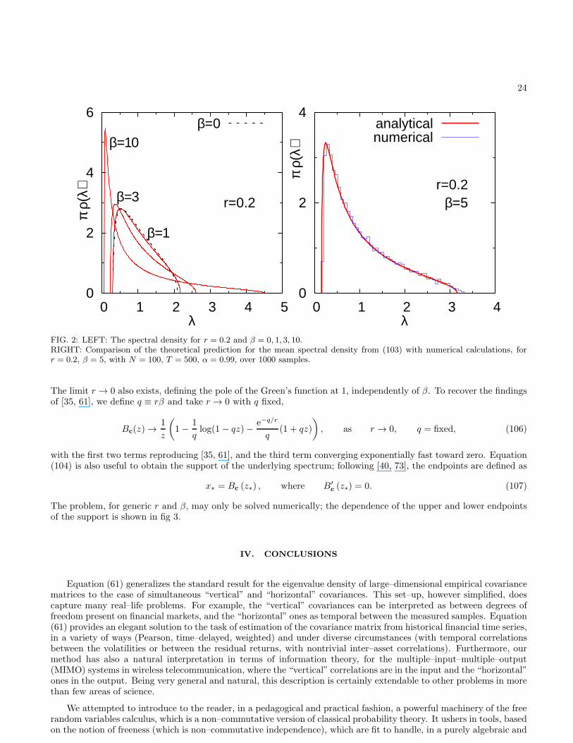
24

0

2

4

6

0 1 2 3 4 5

π ρ

(λ)

λ

β=1

β=3

β=10

r=0.2

β=0

0

2

4

0 1 2 3 4π

ρ(λ

)

λ

r=0.2β=5

analyticalnumerical

FIG. 2: LEFT: The spectral density for r = 0.2 and β = 0, 1, 3, 10.RIGHT: Comparison of the theoretical prediction for the mean spectral density from (103) with numerical calculations, forr = 0.2, β = 5, with N = 100, T = 500, α = 0.99, over 1000 samples.

The limit r → 0 also exists, defining the pole of the Green’s function at 1, independently of β. To recover the findingsof [35, 61], we define q ≡ rβ and take r → 0 with q fixed,

Bc(z) → 1

z

(1 − 1

qlog(1 − qz) − e−q/r

q(1 + qz)

), as r → 0, q = fixed, (106)

with the first two terms reproducing [35, 61], and the third term converging exponentially fast toward zero. Equation(104) is also useful to obtain the support of the underlying spectrum; following [40, 73], the endpoints are defined as

x∗ = Bc (z∗) , where B′c

(z∗) = 0. (107)

The problem, for generic r and β, may only be solved numerically; the dependence of the upper and lower endpointsof the support is shown in fig 3.

IV. CONCLUSIONS

Equation (61) generalizes the standard result for the eigenvalue density of large–dimensional empirical covariancematrices to the case of simultaneous “vertical” and “horizontal” covariances. This set–up, however simplified, doescapture many real–life problems. For example, the “vertical” covariances can be interpreted as between degrees offreedom present on financial markets, and the “horizontal” ones as temporal between the measured samples. Equation(61) provides an elegant solution to the task of estimation of the covariance matrix from historical financial time series,in a variety of ways (Pearson, time–delayed, weighted) and under diverse circumstances (with temporal correlationsbetween the volatilities or between the residual returns, with nontrivial inter–asset correlations). Furthermore, ourmethod has also a natural interpretation in terms of information theory, for the multiple–input–multiple–output(MIMO) systems in wireless telecommunication, where the “vertical” correlations are in the input and the “horizontal”ones in the output. Being very general and natural, this description is certainly extendable to other problems in morethan few areas of science.

We attempted to introduce to the reader, in a pedagogical and practical fashion, a powerful machinery of the freerandom variables calculus, which is a non–commutative version of classical probability theory. It ushers in tools, basedon the notion of freeness (which is non–commutative independence), which are fit to handle, in a purely algebraic and

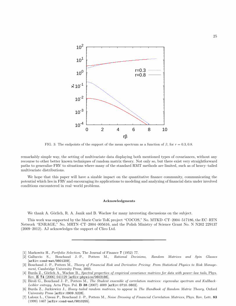
25

10-4

10-3

10-2

10-1

100

101

102

0 2 4 6 8 10

x *

rβ

r=0.3r=0.8

FIG. 3: The endpoints of the support of the mean spectrum as a function of β, for r = 0.3, 0.8.

remarkably simple way, the setting of multivariate data displaying both mentioned types of covariances, without anyrecourse to other better known techniques of random matrix theory. Not only so, but there exist very straightforwardpaths to generalize FRV to situations where many of the standard RMT methods are limited, such as of heavy–tailedmultivariate distributions.

We hope that this paper will have a sizable impact on the quantitative finance community, communicating thepotential which lies in FRV and encouraging its applications to modeling and analyzing of financial data under involvedconditions encountered in real–world problems.

Acknowledgments

We thank A. Gorlich, R. A. Janik and B. Wac law for many interesting discussions on the subject.

This work was supported by the Marie Curie ToK project “COCOS,” No. MTKD–CT–2004–517186, the EC–RTNNetwork “ENRAGE,” No. MRTN–CT–2004–005616, and the Polish Ministry of Science Grant No. N N202 229137(2009–2012). AJ acknowledges the support of Clico Ltd.

[1] Markowitz H., Portfolio Selection, The Journal of Finance 7 (1952) 77.[2] Galluccio S., Bouchaud J.–P., Potters M., Rational Decisions, Random Matrices and Spin Glasses

[arXiv:cond-mat/9801209].[3] Bouchaud J.–P., Potters M., Theory of Financial Risk and Derivative Pricing: From Statistical Physics to Risk Manage-

ment, Cambridge University Press, 2003.[4] Burda Z., Gorlich A., Wac law B., Spectral properties of empirical covariance matrices for data with power–law tails, Phys.

Rev. E 74 (2006) 041129 [arXiv:physics/0603186].[5] Biroli G., Bouchaud J.–P., Potters M., The Student ensemble of correlation matrices: eigenvalue spectrum and Kullback–

Leibler entropy, Acta Phys. Pol. B 38 (2007) 4009 [arXiv:0710.0802].[6] Burda Z., Jurkiewicz J., Heavy–tailed random matrices, to appear in The Handbook of Random Matrix Theory, Oxford

University Press [arXiv:0909.5228].[7] Laloux L., Cizeau P., Bouchaud J.–P., Potters M., Noise Dressing of Financial Correlation Matrices, Phys. Rev. Lett. 83

(1999) 1467 [arXiv:cond-mat/9810255].

26

[8] Plerou V., Gopikrishnan P., Rosenow B., Amaral L. A. N., Stanley H. E., Universal and non–universal properties ofcross–correlations in financial time series, Phys. Rev. Lett. 83 (1999) 1471 [arXiv:cond-mat/9902283].

[9] Laloux L., Cizeau P., Potters M., Bouchaud J.–P., Random Matrix Theory and Financial Correlations, Int. J. Theor. App.Finance 3 (2000) 391.

[10] Plerou V., Gopikrishnan P., Rosenow B., Amaral L. A. N., Guhr T., Stanley H. E., A Random Matrix Approach toCross–Correlations in Financial Data, Phys. Rev. E 65 (2002) 066126 [arXiv:cond-mat/0108023].

[11] Drozdz S., Kwapien J., Grummer F., Ruf F., Speth J., Quantifying dynamics of the financial correlations, Physica A 299

(2001) 144 [arXiv:cond-mat/0102402].[12] Lillo F., Mantegna R. N., Noise dressing of the correlation matrix of factor models [arXiv:cond-mat/0305546].[13] Repetowicz P., Richmond P., The Wick theorem for non–Gaussian distributions and its application for noise filtering of

correlated q–Exponentialy distributed random variables [arXiv:math-ph/0411020].[14] Utsugi A., Ino K., Oshikawa M., Random Matrix Theory Analysis of Cross Correlations in Financial Markets

[arXiv:cond-mat/0312643].[15] Pafka S., Kondor I., Noisy Covariance Matrices and Portfolio Optimization, Eur. Phys. J. B 27 (2002) 277

[arXiv:cond-mat/0111503].[16] Pafka S., Kondor I., Noisy Covariance Matrices and Portfolio Optimization II, Physica A 319 (2003) 487

[arXiv:cond-mat/0205119].[17] Pafka S., Kondor I., Estimated Correlation Matrices and Portfolio Optimization, Physica A 343 (2004) 623

[arXiv:cond-mat/0305475].[18] Papp G., Pafka S., Nowak M. A., Kondor I., Random Matrix Filtering in Portfolio Optimization, Acta Phys. Pol. B 36

(2005) 2757 [arXiv:physics/0509235].[19] Guhr T., Kalber B., A new method to estimate the noise in financial correlation matrices, J. Phys. A 36 (2003) 3009.[20] Malevergne Y., Sornette D., Collective origin of the coexistence of apparent random matrix theory noise and of factors in

large sample correlation matrices, Physica A 331 (2004) 660.[21] Burda Z., Gorlich A., Jarosz A., Jurkiewicz J., Signal and Noise in Correlation Matrix, Physica A 343 (2004) 295

[arXiv:cond-mat/0305627].[22] Burda Z., Jurkiewicz J., Signal and Noise in Financial Correlation Matrices, Physica A 344 (2004) 67

[arXiv:cond-mat/0312496].[23] Burda Z., Jurkiewicz J., Wac law B., Spectral Moments of Correlated Wishart Matrices, Phys. Rev. E 71 (2005) 026111

[arXiv:cond-mat/0405263].[24] Burda Z., Gorlich A., Jurkiewicz J., Wac law B., Correlated Wishart Matrices and Critical Horizons, Eur. Phys. J. B 49

(2006) 319 [arXiv:cond-mat/0508341].[25] Burda Z., Jurkiewicz J., Wac law B., Eigenvalue density of empirical covariance matrix for correlated samples, Acta Phys.

Pol. B 36 (2005) 2641 [arXiv:cond-mat/0508451].[26] Voiculescu D. V., Dykema K. J., Nica A., Free Random Variables, CRM Monograph Series, Vol. 1, Am. Math. Soc.,

Providence, 1992.[27] Speicher R., Multiplicative functions on the lattice of non–crossing partitions and free convolution, Math. Ann. 298 (1994)

611.[28] Burda Z., Janik R. A., Jurkiewicz J., Nowak M. A., Papp G., Zahed I., Free Random Levy Matrices, Phys. Rev. E 65

(2002) 021106 [arXiv:cond-mat/0011451].[29] Burda Z., Jurkiewicz J., Nowak M. A., Papp G., Zahed I., Levy Matrices and Financial Covariances, Acta Phys. Pol. B

34 (2003) 4747 [arXiv:cond-mat/0103108].[30] Burda Z., Jurkiewicz J., Nowak M. A., Papp G., Zahed I., Free Levy Matrices and Financial Correlations, Physica A 343

(2004) 694 [arXiv:cond-mat/0103109].[31] Burda Z., Jurkiewicz J., Nowak M. A., Papp G., Zahed I., Free Random Levy Variables and Financial Probabilities, Physica

A 299 (2001) 181 [arXiv:cond-mat/0103140].[32] Burda Z., Jurkiewicz J., Nowak M. A., Is Econophysics a Solid Science?, Acta Phys. Pol. B 34 (2003) 87

[arXiv:cond-mat/0301096].[33] Burda Z., Jurkiewicz J., Nowak M. A., Papp G., Zahed I., Random Levy Matrices Revisited, Phys. Rev. E 75 (2007)

051126 [arXiv:cond-mat/0602087].[34] Nowak M. A., unpublished talks at:

Exystence, Budapest, June 2004.Noise in Condensed Matter and Complex Systems, Citta del Mare, July 2004.Applications of Random Matrices to Economy and Other Complex Systems, Krakow, May 2005.

[35] Potters M., Bouchaud J.–P., Laloux L., Financial Applications of Random Matrix Theory: Old Laces and New Pieces,Acta Phys. Pol. B 36 (2005) 2767 [arXiv:physics/0507111].

[36] Bouchaud J.–P., Potters M., Financial Applications of Random Matrix Theory: a short review, to appear in The Handbookof Random Matrix Theory, Oxford University Press [arXiv:0910.1205].

[37] Bouchaud J.–P., Laloux L., Augusta Miceli M., Potters M., Large dimension forecasting models and random singular valuespectra, Eur. Phys. J. B 55 (2007) 201 [arXiv:physics/0512090].

[38] Neu P., Speicher R., Spectra of Hamiltonians with generalized single–site dynamical disorder, Z. Phys. B 95 (1994) 101.[39] Gopakumar R., Gross D., Mastering the master field, Nucl. Phys. B 451 (1995) 379.[40] Janik R. A., Nowak M. A., Papp G., Zahed I., Various Shades of Blue’s Functions, Acta Phys. Pol. B 28 (1997) 2949,

and references therein.

27

[41] Tse D. N. C., Hanly S. V., Linear multiuser receivers: effective interference, effective bandwidth and user capacity, IEEETrans. Inf. Theor. 45 (1999) 641.

[42] Muller R. R., A random matrix model of communication via antenna arrays, IEEE Trans. Inf. Theor. 48 (2002) 2495.[43] Tulino A. M., Verdu S., Random Matrix Theory and Wireless Communications, Found. and Trends in Comm. and Inf.

Theory 1 (2004) 1.[44] Simon S. H., Moustakas A. L., Eigenvalue density of correlated complex random Wishart matrices, Phys. Rev. E 69 (2004)

065101.[45] Marcenko V. A., Pastur L. A., Distribution of Eigenvalues for Some Sets of Random Matrices, Math. USSR Sb. 1 (1967)

457.[46] Wishart J., The Generalized Product Momemnt Distribution in Samples from a Normal Multivariate Population, Biometrika

A 20 (1928) 32.[47] Sharpe W. F., Capital asset prices: A theory of market equilibrium under conditions of risk, Journal of Finance 19 (1964)

425.[48] Brinner B. G., Connor G., How much structure is best? A comparison of market model, factor model and unstructured

equity covariance matrices, The Journal of Risk 10 (2008) 3.[49] Noh J. D., Model for correlations in stock markets, Phys. Rev. E 61 (2000) 5981.[50] Tumminello M., Lillo F., Mantegna R. N., Hierarchically nested factor model from multivariate data, Europhys. Lett. 78

(2007) 30006 [arXiv:cond-mat/0511726].[51] Baik J., Ben Arous G., Peche S., Phase transition of the largest eigenvalue for non–null complex sample covariance matrices,

Ann. Probab. 33 (2005) 1643 [arXiv:math/0403022].[52] Zumbach G., The RiskMetrics 2006 methodology, RiskMetrics Group Inc., March 2007 [http://www.riskmetrics.com].[53] Epps T., Comovement of stock prices in the very short run, J. Am. Stat. Assoc. 74 (1979) 291.[54] Bonanno G., Vandewalle N., Mantegna R. N., Taxonomy of Stock Market Indices, Phys. Rev. E 62 (2000) R7615

[arXiv:cond-mat/0001268].[55] Toth B., Toth B., Kertesz J., Modeling the Epps effect of cross correlations in asset prices, Proc. SPIE 6601 (2007) 66010J

[arXiv:0704.3798].[56] Toth B., Kertesz J., The Epps effect revisited [arXiv:0704.1099].[57] Engle R. F., Autoregressive Conditional Heteroscedasticity with Estimates of Variance of United Kingdom Inflation, Econo-

metrica 50 (1982) 987.[58] Engle R. F., Bollerslev T., Modelling the persistence of conditional variances, Econometric Reviews 5 (1986) 1.[59] Bollerslev T., Generalized autoregressive conditional heteroskedasticity, Journal of Econometrics 31 (1986) 307.[60] Hull J. C., Options, Futures, and Other Derivatives, Prentice Hall, Seventh International Edition, 2008.[61] Pafka S., Potters M., Kondor I., Exponential Weighting and Random–Matrix–Theory–Based Filtering of Financial Covari-

ance Matrices for Portfolio Optimization [arXiv:cond-mat/0402573].[62] Svensson J., The asymptotic spectrum of the EWMA covariance estimator, Physica A 385 (2007) 621.[63] J. P. Morgan & Reuters, RiskMetrics — Technical Document, RiskMetrics Group Inc., Fourth Edition, December 1996

[http://www.riskmetrics.com].[64] Mina J., Xiao J. Y., Return to RiskMetrics: The Evolution of a Standard, RiskMetrics Group Inc., April 2001

[http://www.riskmetrics.com].[65] Zumbach G., Volatility processes and volatility forecast with long memory, Quantitative Finance 4 (2004) 70.[66] Zumbach G., The Empirical Properties of Large Covariance Matrices, The RiskMetrics Journal 9 (2009) 31.[67] Silverstein J. W., Bai Z. D., On the Empirical Distribution of Eigenvalues of a Class of Large Dimensional Random

Matrices, Journal of Multivariate Analysis 54 (1995) 175.[68] Silverstein J. W., Bai Z. D., Spectral Analysis of Large Dimensional Random Matrices, Science Press, Beijing, 2006.[69] Thurner S., Biely C., The Eigenvalue Spectrum of Lagged Correlation Matrices, Acta Phys. Pol. B 38 (2007) 4111.[70] Mayya K. B. K., Amritkar R. E., Analysis of delay correlation matrices [arXiv:cond-mat/0601279].[71] Mehta M. L., Random Matrices, Elsevier Ltd., 2004.[72] Eynard B., Random Matrices, lecture notes, 2000 [Saclay-T01/014, CRM-2708].[73] Zee A., Law of addition in random matrix theory, Nucl. Phys. B 474 (1996) 726 [arXiv:cond-mat/9602146].[74] Feller W., An Introduction to Probability Theory and Its Applications, Vols. 1 and 2, John Wiley & Sons, Inc.[75] Cvitanovic P., Lauwers P. G., Scharbach P. N., The planar sector of field theories, Nucl. Phys. B 203 (1982) 385.[76] ’t Hooft G., A planar diagram theory for strong interactions, Nucl. Phys. B 72 (1974) 461.[77] Bercovici H., Pata V., Stable laws and domains of attraction in free probability theory, Ann. of Math. 149 (1999) 1023;

appendix by Biane P.[78] Bercovici H., Voiculescu D. V., Free Convolution of Measures with Unbounded Support, Ind. Univ. Math. J. 42 (1993) 733.[79] Wigner E. P., Characteristic vectors of bordered matrices with infinite dimensions, Ann. Math. 62 (1955) 548.[80] Ben Arous G., Voiculescu D. V., Free extreme values, Annals of Probability 34 (2006) 2037 [arXiv:math/0501274].[81] Biane P., Speicher R., Free diffusions, free entropy and free Fisher information, Annales de l’Institut Henri Poincare B 37

(2001) 581.[82] Janik R. A., Wieczorek W., Multiplying unitary random matrices — universality and spectral properties, J. Phys. A 37

(2004) 6521 [arXiv:math-ph/0312043].[83] Gudowska–Nowak E., Janik R. A., Jurkiewicz J., Nowak M. A., On diffusion of large matrices, New J. Phys. 7 (2005) 54.[84] Janik R. A., Nowak M. A., Papp G., Wambach J., Zahed I., Non–Hermitian random matrix models: Free random variable

approach, Phys. Rev. E 55 (1997) 4100 [arXiv:hep-ph/9609491].

28

[85] Voiculescu D. V., Limit laws for random matrices and free products, Invent. Math. 104 (1991) 201.[86] Graham R., Knuth D., Patashnik O., Concrete Mathematics: A Foundation for Computer Science, Addison–Wesley, 1994.