Central Limit Theorems for Exchangeable Random Variables When Limits Are Scale Mixtures of Normals

543

0894-9840/03/0700-0543/0 © 2003 Plenum Publishing Corporation

Journal of Theoretical Probability, Vol. 16, No. 3, July 2003 (© 2003)

Central Limit Theorems for Exchangeable RandomVariables when Limits are Scale Mixtures of Normals

Xinxin Jiang1 , 2 and Marjorie G. Hahn3

1 Department of Mathematics and Computer Science, Rhodes College, Memphis, Tennessee38112. E-mail: [email protected]

2 To whom correspondence should be addressed.3 Department of Mathematics, Tufts University, Medford, Massachusetts 02155.

Received September 20, 2001; revised January 21, 2003

Central limit theorems for exchangeable random variables are studied whenlimits are scale mixtures of normals. First, necessary and sufficient conditionsare given under the asymptotic tail probability condition for the mixands:

nPw{|t1 | > ebn} `P 0.

Second, when the weak limits have a particular form, i.e., the mixing measurecomes directly from de Finetti’s Theorem, necessary and sufficient conditionsare given. Finally, some applications are discussed.

KEY WORDS: Central limit theorem; exchangeable random variables; scalemixture of normals; stable convergence.

1. INTRODUCTION

Central limit theorems play a crucial role in probability and statistics.Classical central limit theorems assume the random variables are i.i.d. orjust independent but not identically distributed. In reality though, it may behard for a statistician to verify that the collected data is independent. It isoften preferable to assume that the data may be dependent, but the orderof collecting data does not matter. This kind of data has a property calledexchangeability. For exchangeable sequences, a natural candidate for thedistribution of the weak limit of the partial sums is a scale mixture ofnormals. Let Z be a standard normal random variable, independent of a

random variable s. Then the distribution of sZ is said to be a scale mixtureof normals, and its characteristic function is Ee−1

2s 2t 2

. The followingexample shows how easily a scale mixture of normals can arise. Consider asequence of exchangeable random variables {Xi=s · ei, i \ 1} where theei’s are i.i.d. with Ee1=0 and Ee2

1=1 and s is any random variable inde-pendent of all the ei’s. Then

L 1;ni=1 Xi

`n2=L 1s ·

;ni=1 ei

`n20L(s · Z).

The scale mixture of normals model has been widely discussed in eco-nomics, finance, and engineering since it can provide a better fit for certainphenomena. For example, the daily changes of a specific kind of stock areknown to be modelled well by a scale mixture of normals. The results ofthis paper may help to explain why this is to be expected.

A sequence of random variables {Xn, n \ 1} on the probability space(W, F, P) is said to be exchangeable if for each n,

P(X1 [ x1,..., Xn [ xn)=P(Xp(1) [ x1,..., Xp(n) [ xn)

for any permutation p of {1, 2,..., n} and any xi ¥ R, i=1,..., n.By de Finetti’s theorem,(9) an infinite sequence of exchangeable

random variables is conditionally i.i.d. given some s-field. This s-field canbe either the tail s-field T of {Xn, n \ 1} or the s-field G of permutableevents (Ref. 7, Theorem 7.3.3). Furthermore, there exists a regular condi-tional distribution Pw for Xi given G such that for each w ¥ W the coordi-nate random variables {tn — tw

n , n \ 1} (called mixands) of the probabilityspace (R., B., Pw) are i.i.d. (Ref. 7, Corollary 7.3.5). Namely, for alln ¥ N and xi ¥ R, i=1,..., n,

P(X1 [ x1,..., Xn [ xn)=FW

Dn

i=1P(Xi [ xi | G) dP=F

W

Dn

i=1Pw(ti [ xi) dP.

(1.1)

Hence for each natural number n, any Borel function f: Rn0 R, and

B ¥ B(R) — the Borel sets on (−., +.),

P(f(X1,..., Xn) ¥ B)=FW

P(f(X1,..., Xn) ¥ B | G) dP

=FW

Pw(f(t1,..., tn) ¥ B) dP.

544 Jiang and Hahn

Two trivial examples are i.i.d. random variables and totally determinedrandom variables ({X, X,...}). Two nontrivial but simple examples are{X+ei, i \ 1} and {Y · ei, i \ 1} where the ei’s are i.i.d. and independent ofX or Y, respectively.

Since exchangeability is a natural generalization of i.i.d., central limittheorems for exchangeable sequences have received substantial attention.For example, Blum et al.(5) show that if EX1=0 and EX2

1=1, thenL(;n

i=1 Xi/`n) 0 N(0, 1) if and only if Cov(X1, X2)=0=Cov(X21, X2

2).Unlike the i.i.d. case, a central limit theorem may also hold under thenormalization 1/n. Specifically, Teicher(23) shows that if EX1=0 andCov(X1, X2)=m2 > 0, then L(;n

i=1 Xi/nm) 0 N(0, 1) if and only ifEX1X2 · · · Xk exists and coincides with the kth moment of a standardnormal distribution for all k \ 1. An extreme example occurs, when all Xi’sare the same standard normal random variables, i.e., Xi — Z ’ N(0, 1), -i.Assuming no moments on the Xi’s, Klass and Teicher(17) have the followingresult:

Theorem 1.1 (Ref. 17, Theorem 2). Let {Xn, n \ 1} be a sequence ofexchangeable random variables. For constants an, bn with 0 < bn 0 .,

L 1;ni=1 Xi − an

bn

20 N(0, 1) (1.2)

if and only if there exists a positive sequence en a 0 such that

nPw(|t1 | > enbn) `P 0 (1.3)

and either bn/`n is slowly varying with

vn(w)bn

`P 1,

an(w) − an

bn`

P 0 (1.4)

or bn/n is slowly varying with

vn(w)bn

`P 0, L 1an(w) − an

bn

20 N(0, 1), (1.5)

where

an(w)=nEw t1I(|t1 | [ enbn) (1.6)

Central Limit Theorems 545

and

v2n(w)=n[Ewt2

1I(|t1 | [ enbn) − (Ewt1I(|t1 | [ enbn))2]. (1.7)

Case I (when (1.3) and (1.4) hold) characterizes the situation when theclassical central limit theorem holds for the mixands (see also Remark 3.3for more accurate language). Case II (when (1.3) and (1.5) hold) charac-terizes the situation when the law of large numbers holds for the mixandsand those limits have a standard normal distribution.

If vn(w)/bn converges to a random variable y(w) in (1.4) rather thanthe constant 1, is it possible to say anything? Of course the weak limit willno longer be normally distributed. Instead, it will be a scale mixture ofnormals.

Convergence to a scale mixture of normals when the random variablesare uncorrelated and have finite second moments is first considered inTaylor et al. (22) Without moment assumptions, Hahn and Zhang(16) studythe relationship between the central limit theorem and convergence toa scale mixture of normals when the ti’s are symmetric (hence Xi’s aresymmetric also), as the following theorems show:

Theorem 1.2 (Ref. 16, Theorem 2.1). Let t1 be symmetric. Suppose,bn ‘ . such that

L 1Sn

bn

20L(W)=L(sZ) (1.8)

for s(w) > 0 a.s. and -C1 > 0, ,C2 > 0, such that

FW

s(w) exp 1C2k ln k −C1k2

s2(w)2 dP 0 0 as k 0 0. (1.9)

Then there exists en a 0 such that

nPw(|t1 | > enbn) `P 0 (1.3)

holds and

vn(w)bn

`L y(w) with L(yZ)=L(sZ). (1.10)

Theorem 1.3 (Ref. 16, Theorem 2.2). Assume that t1 is symmetric.Suppose there exist bn ‘ . and en a 0 such that

nPw(|t1 | > enbn) `P 0 (1.3)

546 Jiang and Hahn

and

vn(w)bn

`P s(w). (1.11)

Then (1.8) holds.

Notice that there is a gap between (1.10) and (1.11).There are also results on stable convergence in the central limit

theorems for exchangeable random variables. For example, Cheng andChow(6) prove stable convergence assuming that EX1=0, Et1=0,EX2

1 < ., and Et21 < C for some positive real number C. Mancino and

Pratelli(19) study sufficient conditions for the central limit theorem forweighted sums for a self-centered triangular array of exchangeable randomvariables in Hilbert space. Their condition for convergence to the mixingrandom variable s is very similar to (1.11), which, as Hahn and Zhang(16)

show, is not necessary for (1.8) to hold. Fortini et al.(13) study the centrallimit problem for partially exchangeable random variables. However, theirresults and proofs are flawed as discussed in Section 2 of this paper.

Our purpose is to study necessary and sufficient conditions for

L 1;ni=1 Xi − an

bn

20L(W) (1.12)

where W is a random variable whose distribution is a scale mixture ofnormals with finite variances, i.e., P(W [ x)=P(sZ [ x) -x ¥ R and therandom variable s has 0 < s < . a.s. One consequence of this study is aresolution of the gap between (1.10) and (1.11) (see Corollary 3.2).

The approach used here is based on Klass and Teicher(17) with theincorporation of some techniques from Hahn and Zhang.(16) Throughout,Z will stand for a standard normal random variable, independent of anyother random variables. Its law will be denoted by N(0, 1) or L(Z),and its distribution function by F(x) for all x ¥ R. W will stand for arandom variable whose distribution is a scale mixture of normals, i.e.,L(W)=L(sZ) with s and Z independent. Convergence in law will bedenoted by `

L and equality in distribution by=D .The main results are contained in Theorems 2.1 and 2.2. Their proofs

and two corollaries are given in Section 3. Section 4 discusses some possibleapplications.

2. MAIN RESULTS

As Klass and Teicher(17) point out, condition (1.3), which is a condi-tion on the tail probability of the mixand t1, is crucial in their proof of


Theorem 1.1. Unfortunately this condition is not generally necessary for(1.12) to hold if there is no restriction on W, as Example 2.1 below indi-cates. (It also gives a counterexample to the necessity parts of Theorems 3and 4 in Fortini et al. (13)) Our first result assumes (1.3).

Theorem 2.1. Let {Xn, n \ 1} be a sequence of exchangeable randomvariables. For constants bn with 0 < bn 0 ., assume that

nPw(|t1 | > enbn) `P 0 (1.3)

for some en a 0. Then, there exist constants an such that

L 1;ni=1 Xi − an

bn

20L(W)=L(sZ) (1.12)

if and only if either bn/`n is slowly varying and there exists a randomvariable y(w), independent of Z, with L(yZ)=L(W) such that

vn(w)bn

`L y(w) and

an(w) − an

bn`

P 0, (2.1)

or bn/n is slowly varying with

vn(w)bn

`P 0 and

an(w) − an

bn`L W, (2.2)

where an(w) and vn(w) are as in (1.6) and (1.7) respectively.

Example 2.1. Let {Yn, n \ 0} be i.i.d. Cauchy random variables andbn=n. Then ;n

i=1 Yibn

=D Y0. It is well known that the Cauchy distribution is ascale mixture of normals (Y0=

D A12 Z where A is a positive stable random

variable with characteristic exponent 1/2 which is independent of Z, seeFeller,(12) p. 196). In this case, G is trivial. Hence

nPw(|t1 | > enbn)=nP(|Y1 | > enbn) ’ 1/en 0 . as en 0 0.

This example also shows that Theorems 3 and 4 in Fortini et al. (13) arenot valid as stated.

Notice that in Example 2.1, the ‘‘mixture’’ s comes from Y0 itself,rather than from de Finetti’s Theorem. To insure that the mixture in theweak limit totally comes from de Finetti’s Theorem, the next theoremassumes a condition which is similar to weak convergence in L1 of thedistribution of the partial sums of the mixands. The definition of weak

548 Jiang and Hahn

convergence in L1 can be found in Aldous and Eagleson(2) and will not bestated here.

Prior to stating our second result, consider the definition of stableconvergence first introduced by Renyi.(21) (See also Aldous andEagleson.(2))

Definition 2.1. Let {Yn, n \ 1} be a sequence of random variables on(W, F, P) converging in distribution to a random variable Y. The conver-gence is called stable if additionally for each continuity point y of Y andany event E ¥ F,

limn 0 .

P({Yn [ y} 5 E)=P({Y [ y} 5 E).

Stable convergence of {Yn, n \ 1} to Y is denoted by Yn `L Y (stably).

Theorem 2.2. Let {Xn, n \ 1} be a sequence of exchangeable randomvariables. Assume that there exist constants an, bn with 0 < bn 0 ., suchthat for all E ¥ F and all x ¥ R,

FE

Pw 1;ni=1 ti − an

bn[ x2 dP 0 F

EPw(s(w) Z [ x) dP=F

EF 1 x

s(w)2 dP.

(2.3)

Then there exist en a 0 such that

nPw(|t1 | > enbn) `P 0 (1.3)

and either bn/`n is slowly varying with

vn(w)bn

`L s(w) stably,

an(w) − an

bn`

P 0 (2.4)

or bn/n is slowly varying and

vn(w)bn

`P 0, P 1an(w) − an

bn[ x, E2

0 FE

F 1 xs(w)

2 dP (2.5)

where an(w) and vn(w) are as defined in (1.6) and (1.7).Conversely, if (1.3) and either (2.4) or (2.5) hold then (2.3) holds.

Condition (2.3) is stronger than the usual G-stable convergencedefined as in Mancino and Pratelli(19) and Cheng and Chow.(6) But their


G-stable convergence does not imply (1.3), as Example 2.1 shows. (Since G

is trivial in Example 2.1, (2.3) reduces to the general central limit theoremwith a scale mixture of normals as limit.) Roughly, (2.3) guarantees thatthe classical central limit theorem holds ‘‘locally’’ for the mixands. Theproof of Theorem 3 in Fortini et al. (13) assumes that the mixture comesfrom de Finetti’s representation but no sufficient condition is provided inthe theorem. In fact, they assume this condition throughout their paperwithout noticing it. The following example shows Fortini et al. (13)’s state-ment ‘‘the class of limiting laws can be characterized in terms of (scale)mixtures of stable laws,’’ is not valid, when {Xi, i \ 1} are exchangeable.In fact, if one only assumes the weak convergence of the laws of(; Xi − an)/bn when Xi’s are exchangeable, then how the weak limit isobtained can be very complicated.

Example 2.2. Let {Yi, \ 0} be i.i.d. Cauchy random variables and Xbe any random variable, independent of all Yi’s. Then {Yi+X, i \ 1} is asequence of exchangeable random variables and

;ni=1 (Yi+X)

n=D Y0+X,

which is not a scale mixture of stable laws in general, i.e., Y0+Z ]D

sY forY stable and s independent of Y.

The following example shows that condition (2.3) is not vacuous.

Example 2.3. For i=1, 2,..., let Xi=eXi where ei’s are independent

standard normal random variables and X is a random variable independentof all the ei’s, with values 1,3,5,7,... Then condition (2.3) holds with an=0,bn=`n. s(w) will be a function of X, with values 1, `Var(Z3),`Var(Z5),...

Outline of the proofs: First, Proposition 3.1 establishes that (2.3)implies (1.3). Second, Proposition 3.2 shows that either (2.1) or (2.2) isnecessary for (1.12) and (1.3) to hold. Third, Proposition 3.3 verifies that(1.3) and either (2.1) or (2.2) are sufficient for (1.12) to hold, whichfinishes the proof of Theorem 2.1. Finally, we prove Theorem 2.2.

3. PROOFS AND COROLLARIES

Proposition 3.1. Under the assumption (2.3) of Theorem 2.2, (1.3)holds.

550 Jiang and Hahn

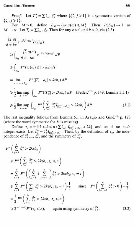
Proof. Let Tgn =;n

j=1 tgj where {tg

j , j \ 1} is a symmetric version of{tj, j \ 1}.

For M > 0, define EM={w: s(w) [ M}. Then P(EM) 0 1 asM 0 .. Let Tn=;n

i=1 ti. Then for any e > 0 and k > 0, via (2.3)

=2p

Mke

e−k 2e 2/2M2P(EM)

\ FEM

=2p

s(w)ke

e−k2e 2/2s(w) 2dP

\ FEM

Pw(|s(w) Z| > ke) dP

= limn 0 .

FEM

Pw(|Tn − an | > kebn) dP

\12

lim supn 0 .

FEM

Pw(|Tgn | > 2kebn) dP (Feller, (12) p. 149, Lemma 5.5.1)

\12

lim supn 0 .

FEM

Pw 1 Cn

j=1tg

j I[|tgj | > ebn] > 2kebn

2 dP. (3.1)

The last inequality follows from Lemma 5.1 in Araujo and Giné,(3) p. 123(where the word symmetric for K is missing).

Define yn=inf{1 [ h [ n : ;hj=1 I[|tg

j | > ebn] \ 2k} and . if no suchinteger exists. Let tg

j =tgj I[|tg

j | > ebn]. Then, by the definition of yn, the inde-pendence of tg

1 ,..., tgn , and the symmetry of tg

j ,

Pw 1 Cn

j=1tg

j > 2kebn2

\ Pw 1 Cn

j=1tg

j > 2kebn, yn [ n2

= Cn

i=1Pw 11 C

i

j=1+ C

n

j=i+1

2 tgj > 2kebn, yn=i2

\ Cn

i=1Pw 1 C

i

j=1tg

j > 2kebn, yn=i2 ·12

since Pw 1 Cn

j=1+1tg

j > 02=12

=12

Pw 1 Cyn

j=1tg

j > 2kebn, yn [ n2

\ 2−(2k+1)Pw(yn [ n), again using symmetry of tgj . (3.2)


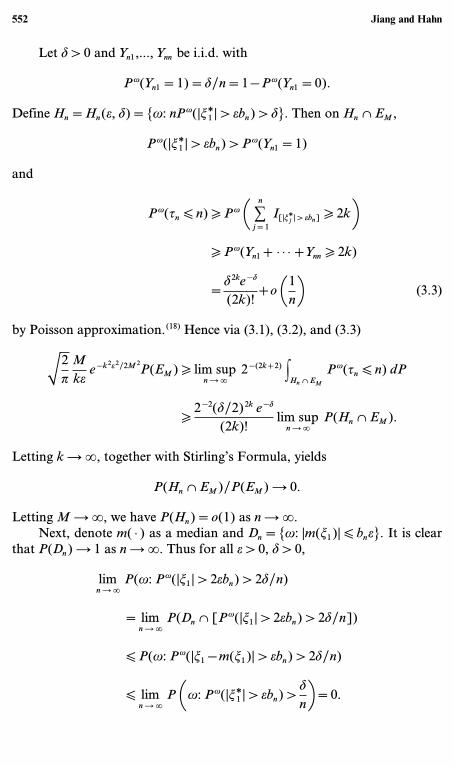
Let d > 0 and Yn1,..., Ynn be i.i.d. with

Pw(Yn1=1)=d/n=1 − Pw(Yn1=0).

Define Hn=Hn(e, d)={w: nPw(|tg1 | > ebn) > d}. Then on Hn 5 EM,

Pw(|tg1 | > ebn) > Pw(Yn1=1)

and

Pw(yn [ n) \ Pw 1 Cn

j=1I[|tg

j | > ebn] \ 2k2

\ Pw(Yn1+ · · · +Ynn \ 2k)

=d2ke−d

(2k)!+o 11

n2 (3.3)

by Poisson approximation.(18) Hence via (3.1), (3.2), and (3.3)

=2p

Mke

e−k 2e 2/2M2P(EM) \ lim sup

n 0 .

2−(2k+2) FHn 5 EM

Pw(yn [ n) dP

\2−2(d/2)2k e−d

(2k)!lim sup

n 0 .

P(Hn 5 EM).

Letting k 0 ., together with Stirling’s Formula, yields

P(Hn 5 EM)/P(EM) 0 0.

Letting M 0 ., we have P(Hn)=o(1) as n 0 ..Next, denote m( · ) as a median and Dn={w: |m(t1)| [ bne}. It is clear

that P(Dn) 0 1 as n 0 .. Thus for all e > 0, d > 0,

limn 0 .

P(w: Pw(|t1 | > 2ebn) > 2d/n)

= limn 0 .

P(Dn 5 [Pw(|t1 | > 2ebn) > 2d/n])

[ P(w: Pw(|t1 − m(t1)| > ebn) > 2d/n)

[ limn 0 .

P 1w: Pw(|tg1 | > ebn) >

d

n2=0.

552 Jiang and Hahn

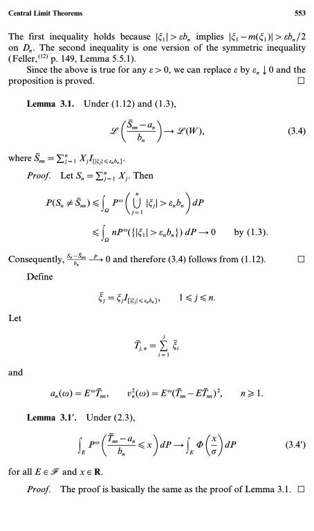
The first inequality holds because |t1 | > ebn implies |t1 − m(t1)| > ebn/2on Dn. The second inequality is one version of the symmetric inequality(Feller,(12) p. 149, Lemma 5.5.1).

Since the above is true for any e > 0, we can replace e by en a 0 and theproposition is proved. i

Lemma 3.1. Under (1.12) and (1.3),

L 1 Snn − an

bn

20L(W), (3.4)

where Snn=;nj=1 XjI[|tj | [ enbn].

Proof. Let Sn=;nj=1 Xj. Then

P(Sn ] Snn) [ FW

Pw 1 0n

j=1|tj | > enbn

2 dP

[ FW

nPw({|t1 | > enbn}) dP 0 0 by (1.3).

Consequently, Sn − Snnbn

`P 0 and therefore (3.4) follows from (1.12). i

Define

tj=tjI[|tj| [ enbn], 1 [ j [ n.

Let

Tj, n= Cj

i=1ti

and

an(w)=EwTnn, v2n(w)=Ew(Tnn − ETnn)2, n \ 1.

Lemma 3.1Œ. Under (2.3),

FE

Pw 1 Tnn − an

bn[ x2 dP 0 F

EF 1x

s2 dP (3.4Œ)

for all E ¥ F and x ¥ R.

Proof. The proof is basically the same as the proof of Lemma 3.1. i


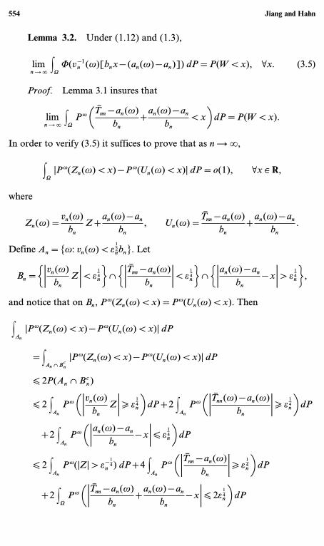
Lemma 3.2. Under (1.12) and (1.3),

limn 0 .

FW

F(v−1n (w)[bnx − (an(w) − an)]) dP=P(W < x), -x. (3.5)

Proof. Lemma 3.1 insures that

limn 0 .

FW

Pw 1 Tnn − an(w)bn

+an(w) − an

bn< x2 dP=P(W < x).

In order to verify (3.5) it suffices to prove that as n 0 .,

FW

|Pw(Zn(w) < x) − Pw(Un(w) < x)| dP=o(1), -x ¥ R,

where

Zn(w)=vn(w)

bnZ+

an(w) − an

bn, Un(w)=

Tnn − an(w)bn

+an(w) − an

bn.

Define An={w: vn(w) < e12nbn}. Let

Bn=3 :vn(w)bn

Z : < e14n4 5 3 :Tnn − an(w)

bn

: < e14n4 5 3 :an(w) − an

bn− x : > e

14n4 ,

and notice that on Bn, Pw(Zn(w) < x)=Pw(Un(w) < x). Then

FAn

|Pw(Zn(w) < x) − Pw(Un(w) < x)| dP

=FAn 5 Bc

n

|Pw(Zn(w) < x) − Pw(Un(w) < x)| dP

[ 2P(An 5 Bcn)

[ 2 FAn

Pw 1 :vn(w)bn

Z : \ e14n2 dP+2 F

An

Pw 1 :Tnn(w) − an(w)bn

: \ e14n2 dP

+2 FAn

Pw 1 :an(w) − an

bn− x : [ e

14n2 dP

[ 2 FAn

Pw(|Z| > e−14

n ) dP+4 FAn

Pw 1 :Tnn − an(w)bn

: \ e14n2 dP

+2 FW


+an(w) − an

bn− x : [ 2e

14n2 dP

554 Jiang and Hahn

[ o(1)+4 FAn

e−12

n

v2n(w)b2

n

dP+2P(W [ x+2e14n) − 2P(W [ x − 2e

14n)

by Chebyshev’s inequality and Lemma 3.1,

[ o(1)+4 FAn

e12n dP=o(1).

The third inequality above holds because

FAn

Pw 1 :an(w) − an

bn− x : [ e

14n2 dP

=FAn

Pw 1 :an(w) − an

bn− x : [ e

14n, :Tnn − an(w)

bn

: > e14n2 dP

+FAn

Pw 1 :an(w) − an

bn− x : [ e

14n, :Tnn − an(w)

bn

: [ e14n2 dP

[ FAn


: \ e14n2 dP

+FAn


+an(w) − an

bn− x : [ 2e

14n2 dP.

Recall the definition of ti and Tnn given after the proof of Lemma 3.1.The next lemma will allow the proof of Lemma 3.2 to be completed byusing the Berry–Esseen Theorem.

Lemma 3.3. For every given e0 > 0, ,Ne0such that when n > Ne0

d 1L 1 Tnn − an(w)vn(w)

2 , N(0, 1)2 [ e0, -w ¥ Acn={w: vn(w) \ e

12nbn}

where d( · , · ) is any metric that metrizes weak convergence (e.g., Lévy dis-tance or d3 distance in Araujo and Giné(3)).

Proof. For any w ¥ Acn, define Xn, m=tm − E wtm

vn(w) for 1 [ m [ n. Then

Cn

m=1Xn, m=

Tnn − an(w)vn(w)

.


We check the Lindeberg–Feller conditions:

(i) Cn

m=1EX2

n, m=nEX2n, 1=n Var t1/v2

n(w) — 1;

(ii) -e > 0, Cn

m=1E(|Xn, m |2, |Xn, m | > e)=

nv2

n(w)Var t1I[|t1 − Et1| > evn(w)]

[2n

v2n(w)

e2nb2

nPw(|t1 − EX1(w)| > evn(w)) since |t1 | [ enbn

0 0

since on Acn, b2

n/v2n(w) [ e−1

n which implies that e2nb2

n/v2n(w) 0 0 as

en a 0, and Pw(|t1 − Et1 | > evn(w)) [Var t1

e2v2n(w)

=v2

n(w)/ne2v2

n(w)0 0.

Thus, by the Lindeberg–Feller Theorem, the lemma holds. i

Returning to the proof of Lemma 3.2, let xn(w)=bnx − an(w)+anvn(w) . Then by

the Berry–Esseen Theorem (Feller,(12) p. 542, Lemma 16.5.1),

FAc

n

|Pw(Zn(w) < x) − P(Un(w) < x)| dP

=FAc

n

:Pw(Z < xn(w)) − Pw 1 Tnn − an(w)vn(w)

< xn(w)2: dP

[ FAc

n

3nEw |t1 − Ewt1 |3

v3n(w)

dP

[ FAc

n

6enbn

vn(w)dP [ 6e

12n=o(1).

Hence the proof of Lemma 3.2 is complete. i

Lemma 3.2Œ. Under assumption (2.3),

limn 0 .

FE

F(v−1n (w)[bnx − (an(w) − an)]) dP=F

EF 1 x

s(w)2 dP (3.5Œ)

holds for all real x ¥ R and all E ¥ F.

556 Jiang and Hahn

Proof. The proof is essentially the same as the proof of Lemma 3.2. i

Lemma 3.4. When (1.12) and (1.3) hold, { vn(w)bn

, n \ 1} and { an(w) − anbn

,n \ 1} are tight.

Proof. Let sn=vn(w)bn

and gn=an(w) − anbn

. Define a random measurean( · , · ) as follows,

an(w, C)=Pw(snZ+gn ¥ C)=L(snZ+gn)(C)

for any w ¥ W and any set C ¥ B(R). Also define

an(C)=Ean( · , C)=FW

an(w, C) dP.

Since limn 0 . an=limn 0 . >W L(sn(w) Z+gn(w)) dP=L(W)byLemma3.2,the sequence {an} is tight. Hence {L(an)} is tight by Lemma 7.14 inAldous.(1)

Suppose sn(w) is not tight, i.e., there exists e0 > 0, such that for anyk ¥ N there exists nk ¥ N with P(Bnk

) :=P{w: snk\ k} \ 2e0. Let An=

{w: an(w) \ an}. Then either P{Ank5 Bnk

} \ e0 or P{Acnk

5 Bnk} \ e0.

Suppose the first inequality holds. Then snk\ k and gnk

\ 0 wheneverw ¥ Ank

5 Bnk. Hence for every x > 0 and w ¥ Ank

5 Bnk,

Pw(snkZ+gnk

[ x) [ Pw(snkZ [ x) [ Pw(kZ [ x)=F 1x

k2 .

Let {bi: i \ 1} be a dense subset in P(B), the probability measureson B. (The existence of such a dense subset is guaranteed by the factthat P(B) is Polish for the weak topology.) Define the ball B(b, d0)={c ¥ P(B) : r(c, b) < d0} where 0 < d0 < 1/8 and r is the Lévy distance onP(B).

The tightness of {L(an)} insures that there exists a compact setKe0

… P(B) such that

P{w: an(w, · ) ¥ Kce0

} < e0 for all n, (3.6)

and there exist bi ¥ P(R), i=1,..., m with 1mi=1 B(bi, d0) ‡ Ke0

. Pickx0 > 0, such that bi(−., x0] \ 1 − d0, i=1,..., m. Since F(x0/k) 0 1

2 ask 0 ., it is possible to choose k0 such that for all k \ k0, F(x0/k)[ 1 − 2d0. Then for w ¥ Ank

5 Bnk, r(bi, ank

(w)) \ d0, i=1,..., m, sinceP(ank

(w)(−., x0]) [ F(x0/k) [ 1 − 2d0. Therefore,


P{w: ank(w) ¥ Kc

e0} \ P 3w: ank

(w) ¥ 3m

i=1Bc(bi, d0)4

=P{w: r(ank(w), bi) \ d0, i=1,..., m}

\ P{Ank5 Bnk

} \ e0,

which contradicts (3.6).Similarly, if P{Ac

nk5 Bnk

} \ e0, by letting x < 0,

Pw(snkZ+gnk

[ x) \ Pw(snkZ [ x) \ Pw(kZ [ x)=F 1x

k2 .

Pick x0 < 0 such that bi(−., x0] < d0, i=1,..., m and k0 such thatF(x0/k) \ 2d0 for all k \ k0. Proceeding as above again yields a contradic-tion. Hence {vn(w)

bn, n \ 1} is tight.

To verify the second portion of the lemma, let Dn+(C)={w:an(w) − an > Cbn} and suppose that there were positive sequences nk ‘ .,Ck ‘ ., and d > 0, such that P{Dnk+(Ck)} > d, k \ 1. Define Gn={w:vn(w) \ bnM} and choose M such that for n large enough, P(Gn) < d/2.Let x > 0, from Lemma 3.2,

2P(W [ x) − 1

= limn 0 .

FW

Pw(|vn(w) Z+an(w) − an | < bnx) dP

[ P{Dcnk+(Ck)}+lim sup

k 0 .

FDnk+(Ck)

Pw(|vnk(w) Z+ank

(w) − ank| < bnk

x) dP

[ 1 − d+lim supk 0 .

FDnk+(Ck) 5 Gc

nk

Pw(|vnk(w) Z+ank

(w) − ank| < bnk

x) dP+d/2

[ 1 − d/2+lim supk 0 .

FDnk+(Ck) 5 Gc

nk

Pw(vnk(w) Z < bnk

x − Ckbnk) dP

[ 1 − d/2+lim supk 0 .

F 1x − Ck

M2=1 − d/2

since on Gcnk

, bnk/vnk

(w) > 1/M, and when Ck is big enough, x − Ck < 0,hence (x − Ck) bnk

/vnk< (x − Ck)/M. Letting x 0 . yields a contradiction.

Similarly, it’s impossible that there are positive sequences nk ‘ .,Ck ‘ ., and d > 0, such that P{w: ank

(w) − ank< − Ck} > d, k \ 1.

This finishes the proof. i

558 Jiang and Hahn

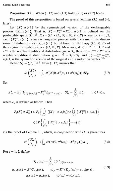
Proposition 3.2. When (1.12) and (1.3) hold, (2.1) or (2.2) holds.

The proof of this proposition is based on several lemmas (3.5 and 3.6,later).

Let {Xgn , n \ 1} be the symmetrized version of the exchangeable

process {Xn, n \ 1}. That is, Xgn =X(1)

n − X (2)n , n \ 1 is defined on the

probability space (W, F, P2)=(W1 × W2, F1 ×F2, P × P) where for i=1, 2,each {X(i)

n , n \ 1} is an exchangeable process with the same finite dimen-sional distributions as {Xn, n \ 1} but defined on the copy (Wi, Fi, P) ofthe original probability space (W, F, P). Moreover, if Ti=T, i=1, 2 andPwi is the regular conditional distribution given Ti, then Pw

2 =Pw1 × Pw2 is aregular conditional distribution given T=T1 ×T2 and tw

n =t w1n − t w2

n ,n \ 1, is the symmetric version of the original i.i.d. random variables.(17)

Define Sgn =;n

j=1 Xgj . Now (1.12) insures that

L 1Sgn

bn

20 F

W

L(N(0, s2(w1)+s2(w2))) dP2. (3.7)

Set

Xgjn=X(1)

j I[|X(1)j | [ enbn] − X (2)

j I[|X(2)j | [ enbn], Sg

kn= Ck

j=1Xg

jn, 1 [ k [ n,

where en is defined as before. Then

P2(Sgn ] Sg

nn) [ P23 0

n

j=1[|X (1)

j | > enbn] 2 0n

j=1[|X (2)

j | > enbn]4

[ 2P 3 0n

j=1[|X(1)

j | > enbn]4=o(1)

via the proof of Lemma 3.1, which, in conjunction with (3.7) guarantees

L 1Sgnn

bn

20 F

W

L(N(0, s2(w1)+s2(w2))) dP2. (3.8)

For i=1, 2, define

Tk, n(wi)= Ck

j=1t wi

j I[|twij | [ enbn],

ak, n(wi)=Ewi Tk, n(wi), v2k, n=Ewi(Tk, n(wi) − ak, n(wi))2,

an(wi)=ann(wi), v2n(wi)=v2

nn(wi).

(3.9)


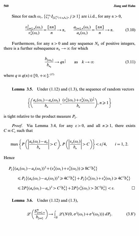
Since for each wi, {t wij I[|twi

j | [ enbn], j \ 1} are i.i.d., for any a > 0,

v2[an], n(wi)v2

n(wi)=

[an]n

0 a,a[an], n(wi)

an(wi)=

[an]n

0 a. (3.10)

Furthermore, for any a > 0 and any sequence Nk of positive integers,there is a further subsequence nk 0 . for which

b[ank]

bnk

0 qa12 as k 0 . (3.11)

where q — q(a) ¥ [0, +.]. (17)

Lemma 3.5. Under (1.12) and (1.3), the sequence of random vectors

31an(w1) − an(w2)bn

,(v2

n(w1)+v2n(w2))

12

bn

2 , n \ 14

is tight relative to the product measure P2.

Proof. Via Lemma 3.4, for any e > 0, and all n \ 1, there existsC — Ce such that

max 3P 1 :an(wi) − an

bn

: > C2 , P 1 :vn(wi)bn

: > C24 < e/4, i=1, 2.

Hence

P2{(an(w1) − an(w2))2+(v2n(w1)+v2

n(w2)) \ 8C2b2n}

[ P2{(an(w1) − an(w2))2 \ 4C2b2n}+P2{v2

n(w1)+v2n(w2) \ 4C2b2

n}

[ 2P{(an(w1) − an)2 > C2b2n}+2P{v2

n(w1) > 2C2b2n} < e. i

Lemma 3.6. Under (1.12) and (1.3),

L 1Sg[an], n

b[an]

20 F

W

L(N(0, s2(w1)+s2(w2))) dP2. (3.8Œ)

560 Jiang and Hahn

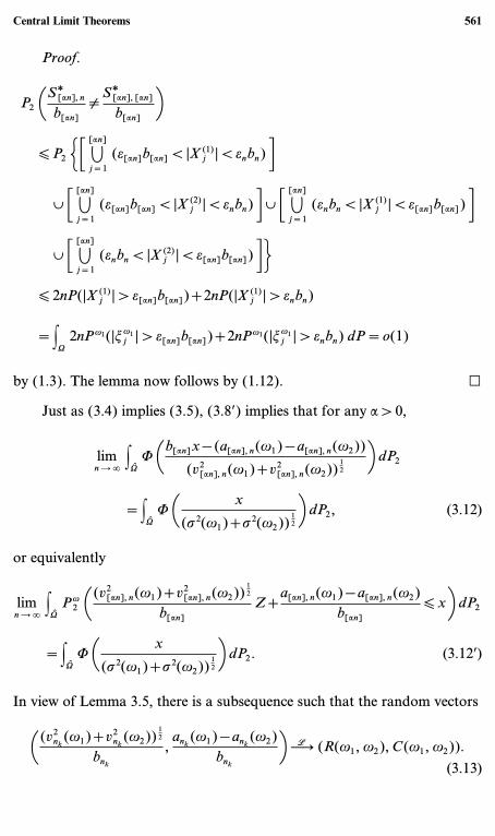
Proof.

P21Sg

[an], n

b[an]]

Sg[an], [an]

b[an]

2

[ P2350

[an]

j=1(e[an]b[an] < |X (1)

j | < enbn)6

2 50[an]

j=1(e[an]b[an] < |X (2)

j | < enbn)6 2 50[an]

j=1(enbn < |X (1)

j | < e[an]b[an])6

2 50[an]

j=1(enbn < |X (2)

j | < e[an]b[an])64

[ 2nP(|X (1)j | > e[an]b[an])+2nP(|X (1)

j | > enbn)

=FW

2nPw1(|t w1j | > e[an]b[an])+2nPw1(|t w1

j | > enbn) dP=o(1)

by (1.3). The lemma now follows by (1.12). i

Just as (3.4) implies (3.5), (3.8Œ) implies that for any a > 0,

limn 0 .

FW

F 1b[an]x − (a[an], n(w1) − a[an], n(w2))

(v2[an], n(w1)+v2

[an], n(w2))12

2 dP2

=FW

F 1 x

(s2(w1)+s2(w2))12

2 dP2, (3.12)

or equivalently

limn 0 .

FW

Pw21 (v2

[an], n(w1)+v2[an], n(w2))

12

b[an]Z+

a[an], n(w1) − a[an], n(w2)b[an]

[ x2 dP2

=FW

F 1 x

(s2(w1)+s2(w2))12

2 dP2. (3.12Œ)

In view of Lemma 3.5, there is a subsequence such that the random vectors

1 (v2nk

(w1)+v2nk

(w2))12

bnk

,ank

(w1) − ank(w2)

bnk

2`L (R(w1, w2), C(w1, w2)).

(3.13)


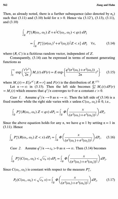
Then, as already noted, there is a further subsequence (also denoted by nk)such that (3.11) and (3.10) hold for a > 0. Hence via (3.12Œ), (3.13), (3.11),and (3.10)

FW

Pw2 (R(w1, w2) Z+a

12 C(w1, w2) < qx) dP2

=FW

Pw2 {(s(w1)2+s2(w2))

12 Z < x} dP2 -x, (3.14)

where (R, C) is a fictitious random vector, independent of Z.Consequently, (3.14) can be expressed in terms of moment generating

functions as

F.

0exp 1 t2r2

2a2 Mr(t) dF(r)=E exp 3q2(s2(w1)+s2(w2))

2at24 (3.15)

where Mr(t)=E{e tC | R=r} and F(r) is the distribution of R. (17)

Let a 0 . in (3.15). Then the left side becomes >.

0 Mr(t) dF(r)=Mr(t) which ensures that q2/a converges to 0 or a constant c > 0.

Case 1. Assume q2/a 0 0 as a 0 .. Then the left side of (3.14) is afixed number while the right side varies with x unless C(w1, w2) —

D 0, i.e.,

FW

Pw2 (R(w1, w2) Z < qx) dP2=F

W

F 1 x

(s2(w1)+s2(w2))12

2 dP2.

Since the above equation holds for any a, we have q — 1 by setting a=1 in(3.11). Hence

FW

Pw2 (R(w1, w2) Z < x) dP2=F

W

F 1 x

(s2(w1)+s2(w2))12

2 dP2. (3.16)

Case 2. Assume q2/a 0 c0 > 0 as a 0 .. Then (3.14) becomes

FW

Pw2 (C(w1, w2) < `c0 x) dP2=F

W

F 1 x

(s2(w1)+s2(w2))12

2 dP2.

Since C(w1, w2) is constant with respect to the measure Pw2 ,

P2(C(w1, w2) < `c0 x)=FW

F 1 x

(s2(w1)+s2(w2))12

2 dP2. (3.17)

562 Jiang and Hahn

Next we show that c0 — 1 in this case by first showing thatR(w1, w2) —

D 0. Let

Rn — R2n(w1, w2)=

v2n(w1)+v2

n(w2)b2

n

.

Then R[ank] ’Rnkq(a) when nk is large. Denote by d( · , · ) any metric that

metrizes weak convergence. Suppose Rnk`L r1 such that d(r1, 0) ] 0. Then

R[ank] 0 r1/q(a)=: ra. Since q2(a)/a 0 c0 > 0 when a 0 ., q(a) 0 ..Hence ra 0 0 as a 0 .. This is equivalent to saying that for any e > 0,,a0 > 1, and nk0

¥ N, such that for all a > a0, nk > nk0,

d(R[ank], 0) < e. (3.18)

On the other hand, Rnk`L r1 and there exists eŒ > 0, with d(r1, 0) > eŒ.

This is equivalent to saying that , n −

k0such that when nk > n −

k0,

d(Rnk, 0) > eŒ. (3.19)

Now choose nk1> max(nk0

, n −

k0) and an integer a1 > a0. Let e=eŒ in (3.18).

Then for nk2=a1nk1

, we have d(R[a1nk1], 0)=d(Rnk2

, 0) < eŒ from (3.18),which contradicts (3.19). So d(r1, 0)=0 which implies Rnk

0 0. Lettinga=1, again by (3.11), q=1. Hence (3.14) together with (3.17) yieldsc0 — 1, which is

P2(C(w1, w2) < x)=FW

F 1 x

(s2(w1)+s2(w2))12

2 dP2. (3.20)

Finally, we show that the weak convergence does not dependent onthe subsequences. Suppose that RnŒk

`L R0 – 0. Then Case 1 applies and

q(a) — 1, -a. Hence

R[anŒk] ’ RnŒk/q(a)=RnŒk

0 R0, -a.

This shows that Rn `L R0 and C(w1, w2)=D 0, i.e., (3.16) gives the limit

distribution along the entire sequence. So in view of Lemma 3.4,

an(w1) − an

bn`

P 0, L 1vn(w1)bn

20L(y(w1))

with FW

L(y(w) Z) dP=L(W).


Suppose that RnŒk`L 0. Then Case 2 applies and R[anŒk] `

L 0, -a. Thisimplies that Rn `

L 0 and (3.20) gives the limit distribution along the entiresequence. Again, in view of Lemma 3.4,

vn(w1)bn

`P 0, L 1an(w1) − an

bn

20L(W).

Furthermore, in Case 2, R(w1, w2)=D 0 and q=`a, hence b[an]/bn

’ a. Consequently, bn/n is slowly varying. In Case 1, q — 1 so b[an]/bn

’ `a and bn/`n is slowly varying. This finishes the proof of Proposi-tion 3.2. i

Proposition 3.3. If (1.3) and either (2.1) or (2.2) hold, then (1.12)holds.

Proof. Since (1.3) holds, it is enough to establish (1.12) with ;ni=1 Xi

replaced by Snn, which is defined in Lemma 3.1.

Case 2. Suppose that (2.2) and (1.3) hold. Using the notationfollowing Lemma 3.1, set

En :={w: Pw(|Tnn − an(w)| > ebn) > d}, d > 0.

By Chebychev’s inequality, Pw(|Tnn − an(w)| > ebn) [ v2n(w)/e2b2

n. Hence

P(En) [ P{v2n(w)/e2b2

n > d}=o(1) as n 0 . by (2.2). (3.21)

Whence

P 1 Snn − an

bn< x2

=FW

Pw 1 Tnn − an

bn< x2 dP

[ FW

Pw 1 Tnn − an

bn< x, :Tnn − an(w)

bn

: [ e2 dP+FW


: > e2 dP

[ FW

Pw 1an(w) − an

bn< x+e2 dP+F

En


: > e2 dP+d

[ P 3w:an(w) − an

bn< x+e4+P(En)+d.

564 Jiang and Hahn

Hence, by (2.2) and (3.21),

lim supn 0 .

P 1 Snn − an

bn< x2 [ P(W < x+e)+d.

Similarly,

lim supn 0 .

P 1 Snn − an

bn\ x2 [ 1 − P(W < x − e)+d,

yielding

lim infn 0 .

P 1 Snn − an

bn< x2 \ P(W < x − e) − d.

The desired conclusion now follows from the continuity of P(W [ x) andthe arbitrariness of both e and d.

Case 1. Suppose (2.1) holds in addition to (1.3). For any e > 0,choose d0 > 0 such that P{w: s(w) [ d0} < e/2. For any 0 < d < d0, set

Dn :=3w: :an(w) − an

bn

: [ d, sn(w) —vn(w)

bn> d4 .

Then P(Dcn) 0 0 as n 0 ..

P 1 Snn − an

bn< x2=F

W

Pw 1 Tnn − an(w)vn(w)

·vn(w)

bn+

an(w) − an

bn< x2 dP

=FW


<bn

vn(w)1x −

an(w) − an

bn

22 dP

[ FDn


<x+d

sn(w)2 dP+P(Dc

n).

Since on Dn, vn(w)/bn > d, by Lemma 3.3 and the Berry–Esseen Theorem,

FDn


<x+d

sn(w)2 dP

=FDn

Pw 1Z [x+d

sn(w)2 dP+o(1)

=FDn

Fx+d

sn(w)

−.

1

`2pe−y 2/2 dy dP+o(1)


=FDn

Fx

−.

1

`2pe−(t+d) 2/2s

2n(w) 1

sn(w)dt dP+o(1)

[ Fx

−.

FW

1

`2pe−(t+d) 2/2s

2n(w) 1

sn(w)dP dt+o(1) using Fubini’s Theorem

=FW

Fx

−.

1

`2pe−(t+d) 2/2y 2(w) 1

y(w)dt dP+o(1) since sn(w) `L y(w)

=FW

F 1x+d

y(w)2 dP+o(1).

Therefore,

lim supn 0 .

P 1 Snn − an

bn< x2 [ F

W

F 1x+d

y(w)2 dP+2e.

Analogously,

lim infn 0 .

P 1 Snn − an

bn< x2 \ F

W

F 1x − d

y(w)2 dP − 2e.

Since >W F(x/y(w)) dP=P(W [ x), the conclusion follows by lettingd 0 0 and e 0 0 . i

Proof of Theorem 2.2. Necessary conditions: Since (2.3) is assumed,Proposition 3.1 guarantees that (1.3) holds and Theorem 2.1 implies thenecessity of the second condition in (2.4) and first one in (2.5). The secondcondition in (2.5) now follows directly from (3.5Œ) and the first conditionin (2.5). To establish the first condition in (2.4), notice that (3.12) holdsfor W replaced by E × E. If a limit theorem is not stable, there exists a sub-sequence along which it will be stable. (This is a statement in Aldous andEagleson.(2) See also the proof of Theorem 3 in Eagleson.(10)) Hence (3.13)holds on E × E for a subsequence of nk (also denoted by nk). Then (3.14)and (3.16) are valid for W replaced by E × E. The same argument showsthat the weak convergence, conditioning on E × E, does not depend on thesubsequences. Thus

L 1 (v2n(w1)+v2

n(w2))1/2

bn

: E × E20L(R(w1, w2) | E × E)

566 Jiang and Hahn

and

L 1vn(w)bn

: E 20L(y(w) | E) (3.22)

where

FE

F 1 xy(w)

2 dP=FE

F 1 xs(w)

2 dP. (3.23)

Let EŒ={w: y(w) < s(w)}. On EŒ,

FEŒ

F 1 xy(w)

2 dP > FEŒ

F 1 xs(w)

2 dP

if P(EŒ) > 0, which contradicts (3.23). Hence P(EŒ)=0. By similar argu-ments, if Eœ={w: y(w) > s(w)} then P(Eœ)=0. So y(w)=s(w) P-a.s.which, together with (3.22), yields the first condition of (2.4).

Sufficient conditions: The proof is virtually the same as the proof ofProposition 3.3 by replacing W with E, Dn with Dn 5 E, Dc

n with Dcn 5 E,

and incorporating Theorem 1Œ in Aldous and Eagleson(2) which ensuresthat g(sn(w)) `L g(s(w)) stably if sn(w) `L s(w) stably and g is a con-tinuous function. i

Remark 3.1. When s(w) is bounded P a.s., the proof of Proposi-tion 3.1 is still valid with EM replaced by W, which yields the followingcorollary:

Corollary 3.1. Assume s(w) is bounded P a.s. Then (1.12) holds ifand only if (1.3) and either (2.1) or (2.2) hold.

Remark 3.2. To insure (1.3) holds, Hahn and Zhang(16) employcondition (1.9). Notice that if s(w) is bounded P a.s., then (1.9) holds. Thefollowing corollary fills the gap between sufficient and necessary conditionsin Hahn and Zhang,(16) namely, between (1.10) and (1.11).

Corollary 3.2. Under (1.9), (1.12) holds if and only if (1.3) andeither (2.1) or (2.2) hold.

Requiring either s(w) to be bounded P a.s. or condition (1.9) restrictsthe tail probability of W. For example, when s(w) is bounded P a.s., thetail probability of W is very similar to that of a normal distribution. But


these conditions are certainly not necessary for (1.12) to hold. For instance,when s(w) has a heavy tail, W will also have a heavy tail but (1.12) or (2.3)can still hold.

Remark 3.3. Recall that a sequence of distributions {Lwn , n \ 1} is

said to converge to Lw in probability if - e > 0, P(w: d(Lwn , Lw) > e)

0 0, as n 0 ., where d( · , · ) is any metric that metrizes the weak conver-gence (Hahn and Zhang,(16) Definition 1.4). Lemma 3.3 shows that

P 3w: L 1;ni=1 ti − an(w)

vn(w)20 N(0, 1)4 \ P 3w:

vn(w)bn

> `en4 .

So if P{w: vn(w)/bn [ `en} 0 0 for some en a 0 (Case 1) then t1 is in thedomain of attraction of a normal in probability. However, Example 3 inKlass and Teicher(17) shows that it is possible that for almost all w ¥ W, tw

1

does not belong to the domain of attraction of any law even though thepartial sum of the original exchangeable random variables can still becentered and scaled to converge weakly to a normal random variable. Thatis why we can not find a set to replace Ac

n in Lemma 3.3 which has positivemeasure and is independent of n.

4. APPLICATIONS

Exchangeable random variables appear in many statistical applica-tions. Three examples of applications of exchangeable sequences of normalrandom variables are given in Tong(24) (p. 114): (1) Random-effects modelsin ANOVA problems; (2) Distribution of a data variable in the Bayestheory; (3) Simultaneous comparisons of normal means with a control.Mixtures of normals are widely used in economics and engineering. Forexample, Fama(11) uses a mixture of normals model to explain the heavytail of the distribution of daily speculative price movements while Grosset al. (14) use a mixture of normals to approximate the equivalent loadduration curves for production costs.

Here we discuss two examples of possible applications of our theory.The examples are given for illustrative purposes only and are not exhaustive.

Example 4.1. Consider the daily price change for a specific stock. Itis known that its distribution has a heavier tail than a normal distribution,which suggests that the classical random walk model is not particularlyappropriate. There are two models frequently proposed to explain theobserved departures from normality, a stable Paretian (Mandelbrot(20))

568 Jiang and Hahn

and a scale mixture of normals distribution (Fama(11)). In Clark(8) a sub-ordinated stochastic process model is applied to modeling cotton futuresprices. The results reported are supportive of the scale mixture of normalsmodel. Though a symmetric stable law is also a scale mixture of normals,the explanations of the heavy tails in these two models are different.Another difference occurs in the variance.

Suppose the daily price change (S) is viewed as a sum of price changes(Xi), each over a short period of time, say one minute. Then the stableParetian model can be formulated as S=;n

i=1 Xi where Xi’s are i.i.d.without finite second moments. The second model (e.g., Clark(8)) can beformulated as S=;Nn

i=1 Xi where Xi’s are i.i.d. with finite second momentsand Nn is a random variable with finite variance which represents the timewhen the nth piece of information occurs. Then the distribution of S is ascale mixture of normals, having finite variance. Recent research providesreasonably strong evidence in favor of the scale mixture of normals models(e.g., Hall et al. (15)).

Since a scale mixture of normal distributions can arise very naturallyas a limiting distribution for sums of exchangeable random variables, wesuggest that Xi’s might be exchangeable. Specifically, let Xi=bei, whereei’s are i.i.d. with mean zero and finite variance, independent of b. Hereb > 0 is a function of the information, e.g., interest rate, earnings, eco-nomic data, political events and natural disasters etc. Xi’s are exchange-able since given the value of b, the random variables bei are i.i.d. LetS=;n

i=1 Xi. To simplify the situation, we assume all information comesbefore the market opens. Recent research for the U.S. Treasury Market(Balduzzi et al. (4)) shows that the impact of the announced informationgenerally occurs within one minute after the announcement, which allowsus to assume that the impact on the trend is negligible in daily changes.This is equivalent to assuming that the impact on the trend is equal to theprice difference between today’s first trade and yesterday’s last trade. Theidea is the following: Given certain (daily) information, the price of acertain stock changes randomly. During intra-day trades, the informationmainly affects the variance of the random variable which represents theprice change in a short period of time (bei here). If there is no significantinformation announced at the beginning of that day, b may be small andtrading may not be very active. If a major economic announcement isreleased, b may be large which represents the high volatility.

The advantage of this model is that there is no assumption that theXi’s have finite second moments. Our result shows that as long as ei’s havefinite second moments, or under even less strict assumptions like (1.3) inthe previous sections of this paper, the partial sums will asymptotically bedistributed as a scale mixture of normal distributions.


Example 4.2. When sending a signal a long distance, errors mayoccur. Hence the signal received on the other side will be the true signalplus an error. Let S be the error of one signal when many signals are sentsimultaneously. Separate the whole distance into a large number of smallintervals of equal length. Denote the error incurred on the ith small inter-val by Xi. Assume the Xi’s are i.i.d. with finite variance. It is also reason-able to assume that when more signals are sent simultaneously, the varian-ces of the errors will increase. Let S be the sum of the small errors, i.e.,S=;n

i=1 Xi. Then S is the total error for one signal in a group of signalssent simultaneously. The Xi might be a function of N and ei, say f(N, ei),where ei’s are i.i.d., representing the error on the ith interval if onlyone signal is sent, and N is a random variable representing the number ofsignals being sent, independent of all ei’s. In this case, (X1, X2,...) formsan exchangeable sequence and the error S can be assumed to be a scalemixture of normals if N only affects the variances of ei’s and f(N, e1) hasfinite second moments for each value of N.

These two examples show how our results might be used to interpretpossible underlying causes for certain observed real world phenomena.

REFERENCES

1. Aldous, D. J. (1983). Exchangeability and Related Topics, Lecture Notes in Mathematics,Springer-Verlag.

2. Aldous, D. J., and Eagleson, G. K. (1978). On mixing and stability of limit theorems.Ann. Probab. 6, 325–331.

3. Araujo, A., and Giné, E. (1980). The Central Limit Theorem for Real and Banach ValuedRandom Variables, Wiley.

4. Balduzzi, P., Elton, E. J., and Green, T. C. (1999). Economic news and bond prices:Evidence from the U.S. treasury market. J. Financ. Quant. Anal. 36(4), 523–543.

5. Blum, J. R., Chernoff, H., Rosenblatt, M., and Teicher, H. (1958). Central limit theoremsfor interchangeable processes. Canad. J. Math. 10, 222–229.

6. Cheng, T. L., and Chow, Y. S. (2002). On stable convergence in the central limit theorem.Statist. Probab. Lett. 57, 307–313.

7. Chow, Y. S., and Teicher, H. (1978). Probability Theory: Independence, Interchangeability,Martingales, Springer, New York.

8. Clark, P. K. (1973). A subordinated stochastic process model with finite variance forspeculative prices. Econometrica 41, 135–155.

9. De Finetti, B. (1937). La Prévision, ses lois logiques, ses sources subjectives. Ann. Inst. H.Poincaré 7, 1–68.

10. Eagleson, G. K. (1967). Some simple conditions for limit to be mixing. Theo. Verojatnost.i Primenen 21, 653–660.

11. Fama, E. F. (1965). The behavior of stock market prices. J. Bus. 38, 34–105.12. Feller, W. (1971). An Introduction to Probability Theory and Its Applications, Vol. II,

Wiley.

570 Jiang and Hahn

13. Fortini, S., Ladelli, L., and Regazzini, E. (1996). A central limit problem for partiallyexchangeable random variables. Theory Probab. Appl. 41(2).

14. Gross, G., Garapic, N. V., and Mcnutt, B. (1988). The mixture of normals approximationtechnique for equivalent load duration curves. IEEE Trans. Power Syst. 3(2), 368–374.

15. Hall, J., Brorsen, B. W., and Irwin, S. (1989). The distribution of futures prices: A test ofthe stable Paretian and mixture of normals hypotheses. J. Financ. Quant. Anal. 24(1),105–116.

16. Hahn, M., and Zhang, G. (1998). Distinctions between the regular and empirical centrallimit theorems for exchangeable random variables. In Progress in Probability, Vol. 43,Birkhäuser Verlag Basel, Switzerland, pp. 111–143.

17. Klass, M., and Teicher, H. (1987). The central limit theorem for exchangeable randomvariables without moments. Ann. Probab. 15, 138–153.

18. Le Cam, L. (1960). An approximation theorem for the Poisson binomial distribution.Pacific J. Math. 10, 1181–1197.

19. Mancino, M. E., and Pratelli, L. (2000). Some results of stable convergence forexchangeable random variables in Hilbert spaces. Theory Probab. Appl. 45(2).

20. Mandelbrot, B. (1963). The variation of certain speculative prices. J. Bus. 36, 394–419.21. Renyi, A. (1963). On stable sequences of events. Sankhya Ser. A 25, 293–302.22. Taylor, R. L., Daffer, P. Z., and Patterson, R. F. (1985). Limit Theorems for Sums of

Exchangeable Random Variables, Rowman & Allanheld.23. Teicher, H. (1971). On interchangeable random variables. In Studi di Probabilita Statistica

e Ricera in onore di Giuseppe Pompilj, pp. 141–148.24. Tong, Y. L. (1990). The Multivariate Normal Distribution, Springer-Verlag.


Central Limit Theorems for Exchangeable Random Variables When Limits Are Scale Mixtures of Normals

Documents

Transcript of Central Limit Theorems for Exchangeable Random Variables When Limits Are Scale Mixtures of Normals