arX

iv:0

901.

3222

v2 [

mat

h.C

V]

4 N

ov 2

011

Corrigendum: Conical plurisubharmonic measure

and new cross theorems

Viet-Anh Nguyen

November 8, 2011

Abstract

In the paper [6] we prove a theorem on the boundary behavior of theconical plurisubharmonic measure. However, the proof turns out to beincomplete. In the present work we give a corrected proof of this theorem.We next apply it to the theory of separately holomorphic functions. Theseapplications are presented in a more accessible way than in [6].

Classification AMS 2010: Primary 32U, 32U05, 32D10, 32D15Keywords: Generic manifold, cross theorem, holomorphic extension, conicalplurisubharmonic measure.

1 Introduction and statement of the main re-

sults

Let D be an open subset of Cn and A ⊂ ∂D. We suppose in addition that D islocally C 2 smooth on A (i.e. for any ζ ∈ A, there exist an open neighborhoodU = Uζ of ζ in Cn and a real function ρ = ρζ ∈ C 2(U) such that D ∩ U = z ∈U : ρ(z) < 0 and dρ(ζ) 6= 0). For ζ ∈ A and 1 < α < ∞, we consider theconical approach region

Aα(ζ) := z ∈ D : |z − ζ | < α · dist(z, Tζ) ,

where dist(z, Tζ) denotes the Euclidean distance from the point z to the tangenthyperplane Tζ of ∂D at ζ.

For any function u defined on D, let

u(z) :=

u(z), z ∈ D,

supα>1

lim supw∈Aα(z), w→z

u(w), z ∈ ∂D.

1

Next, consider the function hA,D := supu∈F

u, where

F := u ∈ PSH(D) : u ≤ 1 on D, u ≤ 0 on A .

Here PSH(D) denotes the set of all functions plurisubharmonic on D. Then theconical plurisubharmonic measure of A relative to D is given by

ω(z, A,D) := h∗A,D(z), z ∈ D, (1)

where u∗ denotes the upper semicontinuous regularization of a function u.A manifoldM ⊂ Cn of class C 2 is said to be generic if, for every point z ∈ M,

the complex linear hull of the tangent space TzM (to M at z) coincides with thewhole space Cn.

The main purpose of this work is to investigate the boundary behavior of theconical plurisubharmonic measure in a special but important case, and thereafterto apply this study to the theory of separately holomorphic mappings. Now weare in the position to state the main result.

Theorem 1.1. Let M ⊂ Cn be a generic manifold of class C 2 and D a domainin Cn such that M ⊂ ∂D and D is locally C 2 smooth on M. Let A ⊂ M be ameasurable subset of positive measure. Then for all density points z relative toA, ω(z, A,D) = 0.

This theorem describes the stable character of the the conical plurisubhar-monic measure ω(·, A,D) along the conical approach regions at all density pointsrelative to A. It sharpens the previous results of A. Sadullaev (see [8]) and B.Coupet (see [1]) where the estimate ω(·, A,D) < 1 on D was obtained. Our proofrelies on the use of families of analytic discs attached to M and on some fineestimates of plurisubharmonic functions.

This paper is organized as follows.

We begin Section 2 by collecting some results of the method of attachinganalytic discs to a generic manifold in the spirit of Coupet’s work [1]. Next, wedevelop necessary estimates for the conical plurisubharmonic measure and thenprove Theorem 1.1. Section 3 concludes the article with various applications ofTheorem 1.1 in the theory of separately holomorphic mappings.

Acknowledgment and comments. The first version of the paper has beenpublished in [6], but fortunately in March 2011 Malgorzata Zajecka (Krakow)found a gap therein. Namely, the author claimed in the proof of Theorem 2.1 in[6] that this theorem should follow implicitly from Theoreme 2 in [1]. However,this claim is not correct. The present version has filled this gap. But the mainidea of the proof is always the same as in [6]. More specifically, we first constructanalytic discs attached to a given generic manifold, and then apply estimates forplurisubharmonic functions. In the construction of analytic discs Theorem 2.1 in

2

[6] has to be replaced by Proposition 2.1 and 2.2 below. Since the subsequentsteps rely on this construction, the details of the proof are different from thosegiven in [6]. However, the strategy as well as the lemmas are almost unchangedin comparison with [6].

The author would like to thank Malgorzata Zajecka for the valuable help.

2 Proof

For x ∈ Rm let |x| denotes its Euclidean norm. For x ∈ Rn and r > 0 letB(x, r) be the Euclidean ball with center x and with radius r. For a C 2 smoothRiemannian manifold M of dimension m let mesM denote the m-dimensionalLebesgue measure on M . When there is no fear of confusion we often write mesinstead of mesM . If M is a smooth submanifold in Rm then we equip M withthe Riemannian metric induced from Rm. For two functions A and B, we use thefollowing conventional notation. We write A . B (or equivalently A = O(B)) ifthere is a constant c > 0 such that |A| ≤ c|B|. We write A ≈ B if A . B

and B . A. Moreover, A = o(B) means that |A||B| → 0 as |B| → 0. For a

differentiable map g : M → N between Riemannian manifolds, let Jacg denotethe Jacobian matrix of g. If, moreover, dimM = dimN then we denote by |Jacg|the determinant of Jacg.

A smooth generic manifold M ⊂ Cn is said to be totally real if dimRM = n.

Our proof will be divided into two cases. In the first one we assume that M istotally real. The second one will treat the general case of M.

To deal with the first case, let M ⊂ Cn be a totally manifold of class C 2. Wemay assume without loss of generality that 0 ∈ M and T0M = Rn (it suffices toperform an affine change of coordinates). In the sequel given z ∈ Cn we oftenwrite z = x+iy with x, y ∈ Rn. M is then defined in a neighborhood of 0 ∈ Cn bythe equation z = x+ ih(x), where h is a function of class C 2 defined in an openneighborhood of 0 ∈ Rn with values in Rn satisfying h(0) = 0 and dh(0) = 0.

A holomorphic disc on a Jordan domain Σ is, by definition, a continuous mapf : Σ → Cn such that f |Σ is holomorphic. A holomorphic disc f is said to beattached to M on an arc Γ ⊂ ∂Σ if f(Γ) ⊂ M.

Let ∆ be the open unit disc in C and T := ∂∆. Let T be the conjugateoperator on L2(T), that is, the operator which associates to every u ∈ L2(T) anelement T (u) ∈ L2(T) such that

∫TT (u) = 0 and that u+ iT (u) is the boundary

value of a holomorphic function on ∆. Let T (u) be the harmonic extension ofT (u) on ∆.

Fix a smooth function φ defined on ∆ harmonic on ∆ such that

• φ = 0 on eiθ ∈ T : |θ| ≤ π2;

• φ < 0 on eiθ ∈ T : π2< |θ| ≤ π;

3

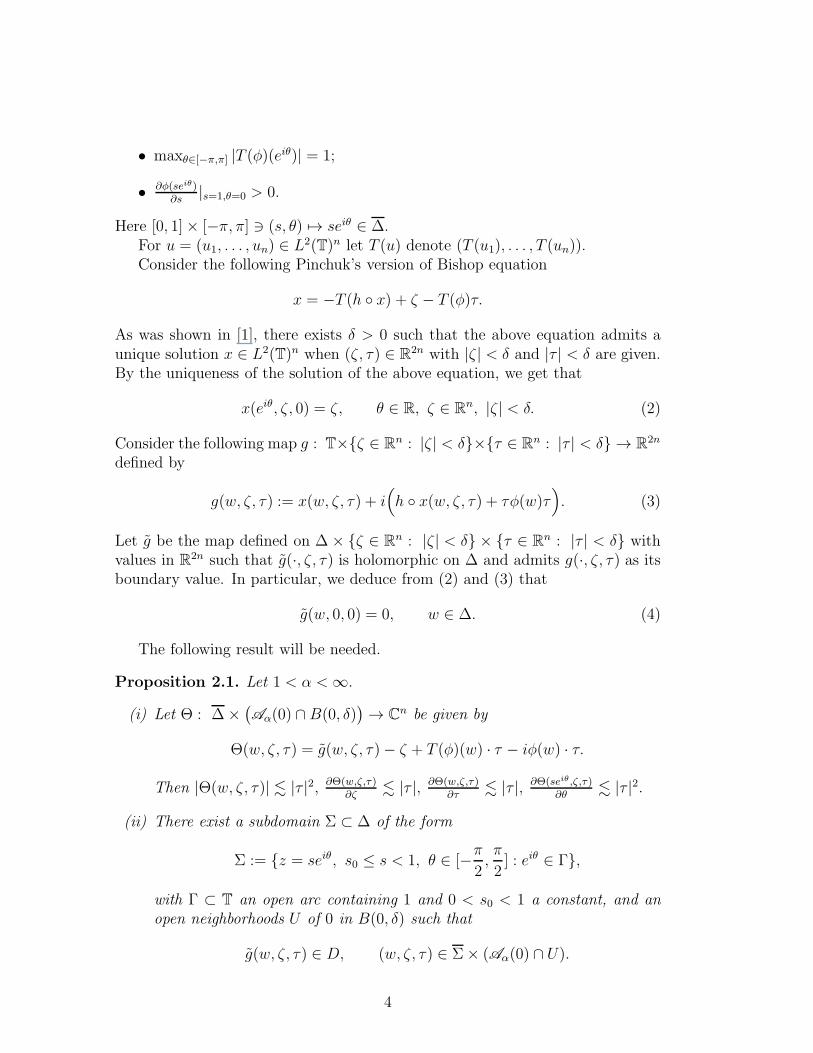
• maxθ∈[−π,π] |T (φ)(eiθ)| = 1;

• ∂φ(seiθ)∂s

|s=1,θ=0 > 0.

Here [0, 1]× [−π, π] ∋ (s, θ) 7→ seiθ ∈ ∆.For u = (u1, . . . , un) ∈ L2(T)n let T (u) denote (T (u1), . . . , T (un)).Consider the following Pinchuk’s version of Bishop equation

x = −T (h x) + ζ − T (φ)τ.

As was shown in [1], there exists δ > 0 such that the above equation admits aunique solution x ∈ L2(T)n when (ζ, τ) ∈ R

2n with |ζ | < δ and |τ | < δ are given.By the uniqueness of the solution of the above equation, we get that

x(eiθ, ζ, 0) = ζ, θ ∈ R, ζ ∈ Rn, |ζ | < δ. (2)

Consider the following map g : T×ζ ∈ Rn : |ζ | < δ×τ ∈ Rn : |τ | < δ → R2n

defined by

g(w, ζ, τ) := x(w, ζ, τ) + i(h x(w, ζ, τ) + τφ(w)τ

). (3)

Let g be the map defined on ∆ × ζ ∈ Rn : |ζ | < δ × τ ∈ Rn : |τ | < δ withvalues in R2n such that g(·, ζ, τ) is holomorphic on ∆ and admits g(·, ζ, τ) as itsboundary value. In particular, we deduce from (2) and (3) that

g(w, 0, 0) = 0, w ∈ ∆. (4)

The following result will be needed.

Proposition 2.1. Let 1 < α <∞.

(i) Let Θ : ∆×(Aα(0) ∩ B(0, δ)

)→ Cn be given by

Θ(w, ζ, τ) = g(w, ζ, τ)− ζ + T (φ)(w) · τ − iφ(w) · τ.

Then |Θ(w, ζ, τ)| . |τ |2, ∂Θ(w,ζ,τ)∂ζ

. |τ |, ∂Θ(w,ζ,τ)∂τ

. |τ |, ∂Θ(seiθ,ζ,τ)∂θ

. |τ |2.

(ii) There exist a subdomain Σ ⊂ ∆ of the form

Σ := z = seiθ, s0 ≤ s < 1, θ ∈ [−π2,π

2] : eiθ ∈ Γ,

with Γ ⊂ T an open arc containing 1 and 0 < s0 < 1 a constant, and anopen neighborhoods U of 0 in B(0, δ) such that

g(w, ζ, τ) ∈ D, (w, ζ, τ) ∈ Σ× (Aα(0) ∩ U).

4

Proof. It follows implicitly from Theoreme 2 in Coupet’s work [1]. For the sakeof clarity we recall briefly his argument.

First recall from estimates (1) and (2) in [1] that

∂g

∂ζ(w, 0, 0) = idζ ,

∂g

∂τ(w, 0, 0) = −T (φ)(w) idτ +iφ(w) idτ .

This, combined with (4) and the formula for Θ, implies that

Θ(w, ζ, τ) = g(w, ζ, τ)− g(w, 0, 0)− ∂g

∂ζ(w, 0, 0)(ζ)− ∂g

∂τ(w, 0, 0)(τ).

On the other hand, for (ζ, τ) ∈ Aα(0) ∩ B(0, δ), we have, by the definition ofconical approach regions, that

|(ζ, τ ′)| < ατn,

where τ = (τ ′, τn). So|ζ | < α|τ |.

This, together with the last identity for Θ, imply all the estimates of Part (i)except the last one. Arguing as in the proof of estimate (3) in [1] and using thelast estimate we can show that, for (ζ, τ) ∈ Aα(0) ∩ B(0, δ),

∂Img

∂s(seiθ, ζ, τ) =

∂φ

∂s(seiθ) · τ + o(τ),

∂Reg

∂s(seiθ, ζ, τ) =

−∂T (φ)∂s

(seiθ) · τ + o(τ).

(5)

This implies that

∂g

∂s(seiθ, ζ, τ) =

∂

∂s

[ζ − T (φ)(w) · τ + iφ(w)τ

]+O(|τ |2).

Hence,∂Θ(w, ζ, τ)

∂s= O(|τ |2).

On the other hand, since Θ(·, ζ, τ) is holomorphic in w, it follows that

∂Θ(w, ζ, τ)

∂θ= is

∂Θ(w, ζ, τ)

∂s.

This, coupled with the last inequality, gives the last estimate of Part (i).

5

Fix α′, α′′ such that 1 < α < α′ < α′′ < ∞. Since D is locally C 2-smooth onA ∋ 0, we may find an open neighborhood U of 0 in Cn such that

Aα′′(z) ∩ U ⊂ D, z ∈ ∂D ∩ U,y + z ∈ Aα′′(z), z ∈ ∂D ∩ U, y ∈ Aα′(0) ∩ U. (6)

On the other hand, estimate (5) for s = 1 gives that

∂Img

∂s(eiθ, ζ, τ) =

∂φ

∂s(eiθ) · τ + o(τ),

∂Reg

∂s(eiθ, ζ, τ) = o(τ),

where the last estimate follows from the identity

∂T (φ)

∂s(eiθ) = −∂φ

∂θ(eiθ) = 0, |θ| < π

2.

Consequently, by shrinking U if necessary we can choose a subdomain Σ ⊂ ∆of the form stated by Part (ii) such that the ray emanating from g(eiθ, ζ, τ) andpassing through g(seiθ, ζ, τ) cuts the unit sphere S (in R2n) at a point η such thatdist(η, ν) = O(|τ |), where

ν :=

(0, ∂φ

∂s(eiθ) · τ

)∣∣∂φ∂s(eiθ) · τ

∣∣ ∈ S.

Moreover, by shrinking Σ if necessary, we may assume that ∂φ

∂s(eiθ) > 0 for

eiθ ∈ Γ. Since this assumption implies that ν ∈ Aα(0), it follows that g(seiθ, ζ, τ)−

g(eiθ, ζ, τ) ∈ Aα′(0) for (ζ, τ) ∈ Aα(0) ∩ B(0, δ) and δ > 0 small enough. So, by(6),

g(seiθ, ζ, τ) ∈ Aα′

(g(eiθ, ζ, τ)

)∩ U ⊂ D, seiθ ∈ Σ.

This completes Part (ii).

Following Theoreme 2 in Coupet’s work [1] we will construct a map G using gand g. This new map is the key ingredient for our proof of Theorem 1.1. Considerthe map (ζ, τ) 7→ g(1, ζ, τ) from an open neighborhood of 0 in R2n toM.We knowfrom estimates (1) and (2) in [1] that the rank of this map is n at 0 ∈ R2n. Sinceg(1, 0, 0) = 0, it follows that there is a C 1 map a defined on an open neighborhoodof 0 in R

n with values in Rn such that

a(0) = 0, and g(1, ζ, τ) = 0 if and only if ζ = a(τ).

Fix a C ∞ map b defined on Rn \ 0 to the space of linear endomorphisms of

rank n − 1 from Rn−1 to Rn such that b(τ)(Rn−1) is orthogonal to τ and that

6

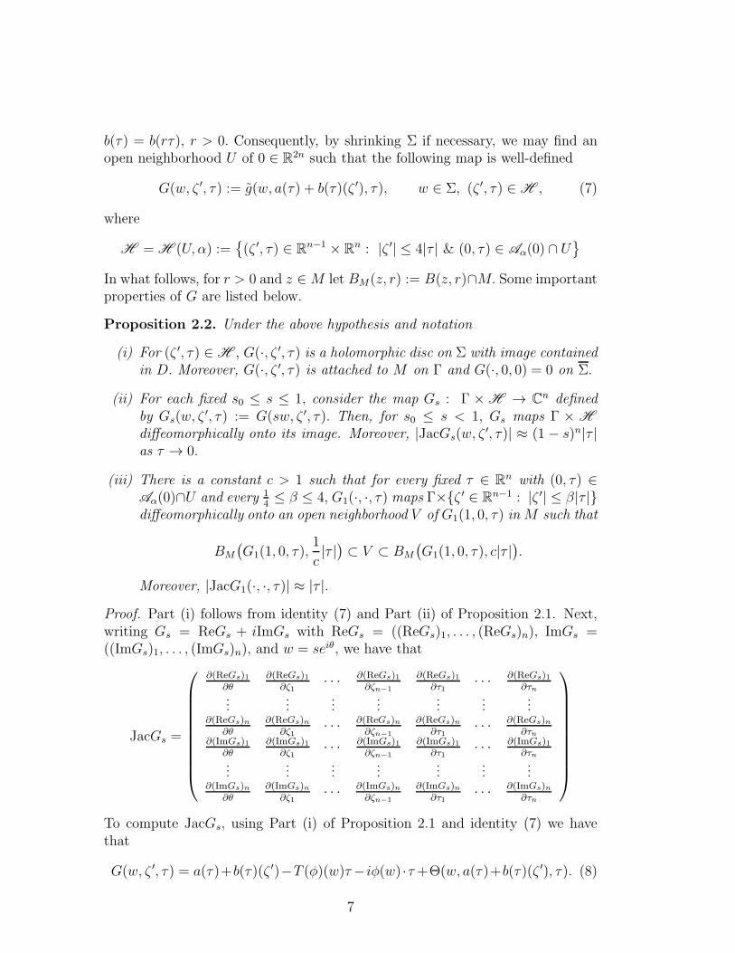
b(τ) = b(rτ), r > 0. Consequently, by shrinking Σ if necessary, we may find anopen neighborhood U of 0 ∈ R2n such that the following map is well-defined

G(w, ζ ′, τ) := g(w, a(τ) + b(τ)(ζ ′), τ), w ∈ Σ, (ζ ′, τ) ∈ H , (7)

where

H = H (U, α) :=(ζ ′, τ) ∈ R

n−1 × Rn : |ζ ′| ≤ 4|τ | & (0, τ) ∈ Aα(0) ∩ U

In what follows, for r > 0 and z ∈M let BM(z, r) := B(z, r)∩M. Some importantproperties of G are listed below.

Proposition 2.2. Under the above hypothesis and notation

(i) For (ζ ′, τ) ∈ H , G(·, ζ ′, τ) is a holomorphic disc on Σ with image containedin D. Moreover, G(·, ζ ′, τ) is attached to M on Γ and G(·, 0, 0) = 0 on Σ.

(ii) For each fixed s0 ≤ s ≤ 1, consider the map Gs : Γ × H → Cn definedby Gs(w, ζ

′, τ) := G(sw, ζ ′, τ). Then, for s0 ≤ s < 1, Gs maps Γ × H

diffeomorphically onto its image. Moreover, |JacGs(w, ζ′, τ)| ≈ (1 − s)n|τ |

as τ → 0.

(iii) There is a constant c > 1 such that for every fixed τ ∈ Rn with (0, τ) ∈Aα(0)∩U and every 1

4≤ β ≤ 4, G1(·, ·, τ) maps Γ×ζ ′ ∈ Rn−1 : |ζ ′| ≤ β|τ |

diffeomorphically onto an open neighborhood V of G1(1, 0, τ) inM such that

BM

(G1(1, 0, τ),

1

c|τ |

)⊂ V ⊂ BM

(G1(1, 0, τ), c|τ |

).

Moreover, |JacG1(·, ·, τ)| ≈ |τ |.

Proof. Part (i) follows from identity (7) and Part (ii) of Proposition 2.1. Next,writing Gs = ReGs + iImGs with ReGs = ((ReGs)1, . . . , (ReGs)n), ImGs =((ImGs)1, . . . , (ImGs)n), and w = seiθ, we have that

JacGs =

∂(ReGs)1∂θ

∂(ReGs)1∂ζ1

· · · ∂(ReGs)1∂ζn−1

∂(ReGs)1∂τ1

· · · ∂(ReGs)1∂τn

......

......

......

...∂(ReGs)n

∂θ

∂(ReGs)n∂ζ1

· · · ∂(ReGs)n∂ζn−1

∂(ReGs)n∂τ1

· · · ∂(ReGs)n∂τn

∂(ImGs)1∂θ

∂(ImGs)1∂ζ1

· · · ∂(ImGs)1∂ζn−1

∂(ImGs)1∂τ1

· · · ∂(ImGs)1∂τn

......

......

......

...∂(ImGs)n

∂θ

∂(ImGs)n∂ζ1

· · · ∂(ImGs)n∂ζn−1

∂(ImGs)n∂τ1

· · · ∂(ImGs)n∂τn

To compute JacGs, using Part (i) of Proposition 2.1 and identity (7) we havethat

G(w, ζ ′, τ) = a(τ)+b(τ)(ζ ′)−T (φ)(w)τ−iφ(w) ·τ+Θ(w, a(τ)+b(τ)(ζ ′), τ). (8)

7

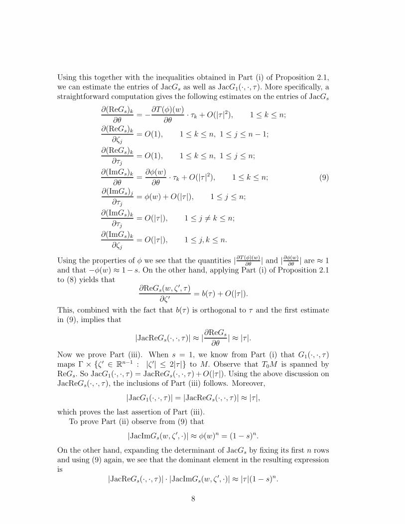
Using this together with the inequalities obtained in Part (i) of Proposition 2.1,we can estimate the entries of JacGs as well as JacG1(·, ·, τ). More specifically, astraightforward computation gives the following estimates on the entries of JacGs

∂(ReGs)k∂θ

= −∂T (φ)(w)∂θ

· τk +O(|τ |2), 1 ≤ k ≤ n;

∂(ReGs)k∂ζj

= O(1), 1 ≤ k ≤ n, 1 ≤ j ≤ n− 1;

∂(ReGs)k∂τj

= O(1), 1 ≤ k ≤ n, 1 ≤ j ≤ n;

∂(ImGs)k∂θ

=∂φ(w)

∂θ· τk +O(|τ |2), 1 ≤ k ≤ n;

∂(ImGs)j∂τj

= φ(w) + O(|τ |), 1 ≤ j ≤ n;

∂(ImGs)k∂τj

= O(|τ |), 1 ≤ j 6= k ≤ n;

∂(ImGs)k∂ζj

= O(|τ |), 1 ≤ j, k ≤ n.

(9)

Using the properties of φ we see that the quantities |∂T (φ)(w)∂θ

| and |∂φ(w)∂θ

| are ≈ 1and that −φ(w) ≈ 1− s. On the other hand, applying Part (i) of Proposition 2.1to (8) yields that

∂ReGs(w, ζ′, τ)

∂ζ ′= b(τ) +O(|τ |).

This, combined with the fact that b(τ) is orthogonal to τ and the first estimatein (9), implies that

|JacReGs(·, ·, τ)| ≈ |∂ReGs

∂θ| ≈ |τ |.

Now we prove Part (iii). When s = 1, we know from Part (i) that G1(·, ·, τ)maps Γ × ζ ′ ∈ Rn−1 : |ζ ′| ≤ 2|τ | to M. Observe that T0M is spanned byReGs. So JacG1(·, ·, τ) = JacReGs(·, ·, τ)+O(|τ |). Using the above discussion onJacReGs(·, ·, τ), the inclusions of Part (iii) follows. Moreover,

|JacG1(·, ·, τ)| = |JacReGs(·, ·, τ)| ≈ |τ |,which proves the last assertion of Part (iii).

To prove Part (ii) observe from (9) that

|JacImGs(w, ζ′, ·)| ≈ φ(w)n = (1− s)n.

On the other hand, expanding the determinant of JacGs by fixing its first n rowsand using (9) again, we see that the dominant element in the resulting expressionis

|JacReGs(·, ·, τ)| · |JacImGs(w, ζ′, ·)| ≈ |τ |(1− s)n.

8

This finishes the proof of Part (ii).

We need the following elementary lemma.

Lemma 2.3. Let Γ be an open arc in T ∩ ∂Σ of the form Γ = eiθ : θ ∈(−2θ0, 2θ0), where 0 < θ0 <

π2is a fixed number. Then there exists 1 < c < ∞

with the following property. If u is a subharmonic function defined in Σ with u ≤ 1on Σ and u ≤ 0 on B, where B is a measurable subset of Γ with mes(Γ\B)

mes(Γ)≤ ǫ2,

then supρ=1−ǫ, |ζ|<θ0u(ρeiζ) ≤ cǫ.

Proof. Let ψ : Σ → ∆ be a conformal map with ψ(1) = 1. Since ψ is smooth on∂Σ ∩∆, we may reduce the problem to the case where Σ = ∆. The assumptionon u implies that for ρ ∈ [0, 1] and ϑ ∈ [−π, π],

u(ρeiϑ) ≤ 1

2π

π∫

−π

(1− ρ2)1B|eiθ − ρeiϑ|2dθ,

where

1B(θ) :=

0, eiθ ∈ B,

1, eiθ 6∈ B.

Therefore, an easy estimate shows that for ρ = 1− ǫ and |ϑ| < θ0.

u(ρeiϑ) ≤ 1

2π

2θ0ǫ2∫

−2θ0ǫ2

(1− ρ2)

|1− ρ|2 dθ +1

2π

∫

|θ|>2θ0

(1− ρ2)

|eiθ − ρeiϑ|2dθ ≤ cǫ.

Suppose without loss of generality that 0 is a point of density relative to A inM. The proof of Theorem 1.1 is divided into several steps. In the first three stepswe assume that M is totally real. Fix arbitrary 0 < ǫ0 < 1 and 1 < α0 <∞. Weonly need to show that there exists a sufficiently small open neighborhood U of0 ∈ Cn such that u(z) ≤ ǫ0 for all z ∈ Aα0

(0) ∩ U and u ∈ F , where the familyF was defined in Section 1.Step 1: Construction of a subset Ωr ⊂ D ∩ B(0, r) for all r > 0 small enoughsuch that u(z) ≤ ǫ0, z ∈ Ωr, u ∈ F .

The idea is to use families of holomorphic discs attached toM which parametrizea open neighborhood of 0 in M. These families are supplied by Proposition 2.2.

For r > 0 let Ur := τ ∈ Rn : r

2≤ |τ | ≤ r and Vr := ζ ′ ∈ R

n−1 : |ζ ′| ≤ 2r.Let γ > 1 and α > α0 be constants large enough whose exact value will bedetermined later on. Since 0 is a point of density relative to A, we may find0 < r0 ≪ 1 such that for all 0 < r < r0,

mes(BM(0, r) \ A

)

mes(BM (0, r)

) < ǫγ0 . (10)

9

Fix 0 < r < r0 and τ ∈ Ur. By Part (iii) of Proposition 2.2, G(·, ·, τ) mapsΓ × Vr diffeomorphically onto an open neighborhood Mτ of 0 in M which is≈ BM(0, r). Moreover, JacG(·, ·, τ) ≈ r. This, combined with (10), implies that

mes(Mτ \ A

)

mes(Mτ )< ǫ

γ0 .

Since Mτ is parametrized by the family of real curves G(Γ, ζ ′, τ) : ζ ′ ∈ Vr, itfollows from the last estimate that

mes(Vr \ V τ

r

)

mes(Vr) < ǫ

γ2

0 , (11)

where

V τr :=

ζ ′ ∈ Vr :

mes(G(Γ, ζ ′, τ) \ A

)

mes(G(Γ, ζ ′, τ)

) < ǫγ2

0

, τ ∈ Ur.

For 0 < ǫ < 1 let Γǫ := (1 − ǫ)eiθ : θ ∈ (−θ0, θ0). Applying Lemma 2.3to the holomorphic discs G(·, ζ, τ)|Σ attached to M on Γ which are supplied byProposition 2.2, we deduce from (11) that

u(z) ≤ cǫ0, z ∈ Ωr, u ∈ F , (12)

whereΩr :=

⋃

τ∈Ur , ζ′∈V τr

G(Γǫ0, ζ′, τ).

Note that by Part (i) of Proposition 2.1 and the above formula for Ωr, we getthat Ωr ⊂ D ∩ B(0, r).Step 2: For 0 < r < r0, let Hr := z = x+ iy ∈ Cn : z ∈ Aα(0), yn ∈ (r, 2r) .Then

mes(Hr \ Ωr)

mes(Hr)≤ ǫ

γ2−n+1

0 .

Consider the setRr :=

⋃

τ∈Ur, ζ′∈Vr

G(Γǫ0, ζ′, τ)

Since V τr ⊂ Vr we clearly have that Ωr ⊂ Rr. Moreover, we deduce from (11) that

mes(Rr \ Ωr)

mes(Rr)< ǫ

γ2

0 . (13)

Next we will introduce a set Sr such that that Aα(0) ∩ Rr ⊂ Sr ⊂ Rr. Forθ ∈ (−θ0, θ0) and τ ∈ Ur, let Vθ,τ be the set of all ζ ′ ∈ Vr such that

|ReG((1− ǫ0)eiθ, ζ ′, τ)| ≤ αǫ0r.

10

To estimate the quotientmes(Vθ,τ )

mes(Vr)observe that

|ReG((1− ǫ0)eiθ, ζ ′, τ)− ReG(1, ζ ′, τ)|

= |Reg((1− ǫ0)eiθ, a(τ) + b(τ)(ζ ′), τ)− Reg(1, a(τ) + b(τ)(ζ ′), τ)

≤(T (φ)((1− ǫ0)e

iθ)− T (φ)(1))τ +O(|τ |2)

. ǫ0r,

where the first inequality follows from Part (i) of Proposition [1]. Moreover, sinceg(1, a(τ), τ) = 0, we get that

|ReG(1, ζ ′, τ)| = |Reg(1, a(τ) + b(τ)(ζ ′), τ)|= |Reg(1, a(τ) + b(τ)(ζ ′), τ)− Reg(1, a(τ), τ)| = b(τ)(ζ ′) +O(|τ |2),

where the last equality also follows from Part (i) of Proposition [1]. This togetherwith the last observation imply that

|ReG((1− ǫ0)eiθ, ζ ′, τ)− b(τ)(ζ ′)| . ǫ0r + O(|τ |2).

Hence, we conclude, for α ≫ 1, that Vθ,τ is approximatively a ball with center 0and radius ǫ0r in Vr. Consequently,

mes(Vθ,τ )

mes(Vr)≈ ǫn−1

0 .

DefineSr := G(Γ0, ζ

′, τ) : τ ∈ Ur, ζ′ ∈ Vθ,τ .

Since Vθ,τ ⊂ Vr, we clearly have that Sr ⊂ Rr. Moreover, using Part (ii) ofProposition 2.2 the last estimate gives that

mes(Sr)

mes(Rr)≈ mes(Vθ,τ )

mes(Vr)≈ ǫn−1

0 . (14)

Using Part (i) of Proposition 2.1 and the estimate

−φ((1− ǫ0)eiθ) ≈ ǫ0, θ ∈ (−θ0, θ0),

we see easily that Aα(0)∩B(0, r) ⊂ Sr. Hence, Aα(0)∩B(0, r) ⊂ Sr ⊂ Rr. This,combined with (13), implies that

mes((Aα(0) ∩ B(0, r) \ Ωr)

mes(Rr)≤ mes(Sr \ Ωr)

mes(Rr)≤ mes(Rr \ Ωr)

mes(Rr)≤ ǫ

γ2

0 .

Using this and (14) and the estimate mes(Aα(0)∩B(0,r))mes(Sr)

≈ 1 it follows that

mes((Aα(0) ∩ B(0, r)) \ Ωr)

mes(Aα(0) ∩B(0, r)). ǫ

γ2−n+1

0 .

11

Since Hr ⊂ Aα(0) ∩ B(0, r) and mes(Aα(0)∩B(0,r))mes(Hr)

≈ 1 the desired conclusion ofStep 2 follows.Step 3: End of the proof of Theorem 1.1 when M is totally real.

First we need some elementary lemmas.

Lemma 2.4. For 0 < a, b < ∞, there exists a constant c > 0 that depends onlyon the quotient a

bwith the following property. Consider the domains

I :=z = x+ iy ∈ C

n : x1, . . . , xn, y1, . . . , yn−1 ∈ (−2b, 2b), yn ∈ (a

2, 4a)

,

J := z = x+ iy ∈ Cn : x1, . . . , xn, y1, . . . , yn−1 ∈ (−b, b), yn ∈ (a, 2a) .

Then, for every u ∈ PSH(I) and every 0 < ǫ < 1 such that u ≤ 1 on I and that

mes(z ∈ I : u(z) ≥ ǫ

2)

mes(I)< cǫ,

we have u < ǫ on J.

Proof. Observe that there exists the maximum number 0 < r < ∞ dependentonly on a and b such that the ball B(z, r) centered at z with radius r in C

n

is contained in I for all z ∈ J. By the sub-mean property of plurisubharmonicfunctions we have

u(z) ≤ 1

mes(B(z, r))

∫

B(z,r)

u(w)dw, z ∈ J.

Setting c := mes(B(z,r))2mes(I)

, we see that c depends only on ab. Moreover, we have that

for every z ∈ J,

mes((z ∈ B(z, r) : u(z) ≥ ǫ

2)

mes(B(z, r))≤ mes(I)

mes(B(z, r))·mes(

(z ∈ I : u(z) ≥ ǫ

2)

mes(I)≤ ǫ

2.

This, combined with the above sub-mean estimate, implies that

u(z) ≤(1− ǫ

2

) ǫ2+ǫ

2< ǫ, z ∈ J.

Lemma 2.5. For every α > 1 there exists a constant c > 0 with the followingproperty. For all a > 0 consider the domains

H :=z = x+ iy ∈ C

n : z ∈ A8√nα(0), yn ∈ (

a

2, 4a)

,

K := z = x+ iy ∈ Cn : z ∈ Aα(0), yn ∈ (a, 2a) .

Then for every u ∈ PSH(H) and every 0 < ǫ < 1 such that u ≤ 1 on H and that

mes(z ∈ H : u(z) ≥ ǫ

2)

mes(H)≤ cǫ,

we have u < ǫ on K.

12

Proof. Applying Lemma 2.4 to the case where b := 2αa and observing thatI ⊂ H, K ⊂ J, the desired conclusion follows.

To prove Theorem 1.1 in the case where M is totally real, let 0 < r < r0 bean arbitrary number. Choose α := 8

√nα0. By Step 2, we get that

u(z) ≤ cǫ0, z ∈ Ωr, u ∈ F ,

where Ωr is a subset of D that satisfies

mes(Hr \ Ωr)

mes(Hr)≤ ǫ

γ2−n+1

0 .

Now it suffices to choose γ ≥ 2n + 1. Then the above quotient is dominated bycǫ0 when ǫ0 is small enough. So we are in the position to apply Lemma 2.5.Consequently, u(z) ≤ ǫ0 for all z = x + iy ∈ Aα0

(0) with yn ∈ (r, 2r). Since0 < r ≪ 1 is arbitrary, this completes the proof.Step 4: The general case.

Let M be a generic manifold of dimension n + k in Cn. By a complex linearchange of coordinates we may assume that T0M = R

n−k × Ck. Let U(k) be the

group of unitary matrices of rank k. For every H ∈ U(k), there is a totallyreal manifold 0 ∋ MH ⊂ M such that T0M

H := Rn−k × H(Rk). Observe thatMH ⊂ M ⊂ ∂D. Since 0 is a point of density relative to A, a slicing argumentshows that we may find 0 < r0 ≪ 1 such that for every 0 < r < r0, there existsan H ∈ U(k) such that

mes(BMH (0, r) \ A

)

mes(BMH(0, r)

) < ǫγ0 .

Using this instead of (10), we argue as in the proof of Steps 1, 2 and 3 above.Consequently, the conclusion of Step 3 and the above observation together implythat

limz→0, z∈Aα(0)

u(z) = 0, u ∈ F , 1 < α <∞.

Hence, the proof of the last step is finished.

3 Applications

The purpose of this section is to derive from Theorem A in our previous work [4]and Theorem 1.1 a boundary cross theorem and a mixed cross theorem. We firstrecall some terminology and notation (relative to the system of conical approachregions) introduced in Section 2 of [4].

Definition 3.1. Let D ⊂ Cm be an open set and A ⊂ D.We say that A is locallypluriregular at a point a ∈ A if one of the following cases happens.

13

• a ∈ D and ω(a, A∩U, U) = 0 for all open neighborhoods U of a in D, whereω(·, A ∩ U, U) is the Siciak relative extremal function.

• a ∈ ∂D and D is locally C 2 smooth on a, and ω(a, A∩∂D∩U,D∩U) = 0for all open neighborhoods U of a, where ω(·, A∩∂D∩U,D∩U) is the conicalplurisubharmonic measure.

Moreover, A is said to be locally pluriregular if it is locally pluriregular at allpoints a ∈ A.

In what follows let M ⊂ Cm be a generic manifold of class C 2 and D an openset in Cm such that M ⊂ ∂D and that D is locally C 2 smooth on M. Now weare in the position to formulate the following version of the plurisubharmonicmeasure.

Definition 3.2. Let M ⊂ Cm be a generic manifold of class C 2 and D a openset in Cm such that M ⊂ ∂D and D is locally C 2 smooth on M. Let A ⊂M. LetA :=

⋃P∈E (A)

P, where

E (A) :=P ⊂M : P is locally pluriregular, P ⊂ A

,

The generalized conical plurisubharmonic measure of A relative to D is the func-tion ω(·, A,D) defined by

ω(z, A,D) := ω(z, A, D), z ∈ D.

The following result is a consequence of Theorem 1.1.

Lemma 3.3. Let A be a measurable subset of M such that mesM(A) > 0. Then

ω(z, A,D) ≤ ω(z, A′, D), z ∈ D,

where A′ is the set of density points of A.

Proof. By Theorem 1.1, A is locally pluriregular at all points of A′. On the otherhand, since mesM(A \ A′) = 0, every point of A′ is also a density point relativeto A′. Hence, A′ is locally pluriregular. Choose an increasing sequence (Ak)

∞k=1

of subsets of A such that Ak is closed and mesM

(A \

∞⋃k=1

An

)= 0. Observe that

A′k is locally pluriregular, A′

k ⊂ Ak ⊂ A Hence, by Definition 3.2 we get that

A :=∞⋃k=1

A′k ⊂ E (A). So

ω(z, A,D) ≤ ω(z, A, D), z ∈ D.

Since mesM(A′ \ A) = 0 we deduce from Theorem 1.1 that

ω(z, A, D) ≤ ω(z, A′, D), z ∈ D.

This, combined with the previous estimate, implies the lemma.

14

Now we are in the position to give two applications of Theorem 1.1. The firstone is a boundary cross theorem.

Theorem 3.4. Let M ⊂ Cm and N ⊂ C

n be two generic manifolds of class C 2.

Let D ⊂ Cm and G ⊂ Cn be two open sets such that M ⊂ ∂D, N ⊂ ∂G and thatD is locally C 2 smooth on M, G is locally C 2 smooth on N. Let A ⊂M, B ⊂ N

be measurable sets such that mesM(A) > 0, mesN (B) > 0. Define

W :=((D ∪A)× B

)⋃(A× (G ∪ B)

),

W ′ := (z, w) ∈ D ×G : ω(z, A′, D) + ω(w,B′, G) < 1 ,

where A′ (resp. B′) is the set of all density points of A (resp. B).Let f : W −→ C be a function which satisfies the following conditions:

• For every a ∈ A, f(a, ·) is holomorphic on G and continuous on G∪B. Forevery b ∈ B, f(·, b) is holomorphic on D and continuous on D ∪ A.

• f is locally bounded, that is, for every x ∈ W, there exist an open neighbor-hood Ux of x in W and a finite constant cx such that supUx

|f | < cx.

• f |A×Bis continuous.

Then there exists a unique holomorphic function f defined on W ′ such that forall 1 < α <∞,

lim(z,w)→(ζ,η), z∈Aα(ζ), w∈Aα(η)

f(z, w) = f(ζ, η), (ζ, η) ∈ A′ × B′;

lim(z,w)→(ζ,η), z∈Aα(ζ)

f(z, w) = f(ζ, η), (ζ, η) ∈ A′ ×G;

lim(z,w)→(ζ,η), w∈Aα(η)

f(z, w) = f(ζ, η), (ζ, η) ∈ D × B′.

If, moreover, supW |f | <∞, then

|f(z, w)| ≤(supA×B

|f |)1−ω(z,A′,D)−ω(w,B′,G)(

supW

|f |)ω(z,A′,D)+ω(w,B′,G)

, (z, w) ∈ W ′.

Proof. Combing Theorem A in [4] and Lemma 3.3, the theorem follows.

The second application is a mixed cross theorem.

Theorem 3.5. Let M ⊂ Cm be a generic manifolds of class C 2. Let D ⊂ Cm

be an open set such that M ⊂ ∂D and that D is locally C 2 smooth on M. LetA ⊂ M be a measurable set such that mesM(A) > 0. Let G ⊂ Cn be an open setand let B be a locally pluriregular subset of G.

15

Define

W :=((D ∪ A)× B

)⋃(A× (G ∪ B)

),

W ′ := (z, w) ∈ D ×G : ω(z, A′, D) + ω(w,B,G) < 1 ,

where A′ is the set of density points of A.Let f : W −→ C be a function which satisfies the following conditions:

• For every a ∈ A, f(a, ·) is holomorphic on G. For every b ∈ B, f(·, b) isholomorphic on D and continuous on D ∪ A.

• f is locally bounded along A×G.

Then there exists a unique holomorphic function f defined on W ′ such that

lim(z,w)→(ζ,η), z∈Aα(ζ)

f(z, w) = f(ζ, η), (ζ, η) ∈ A′ ×G, 1 < α <∞;

lim(z,w)→(ζ,η)

f(z, w) = f(ζ, η), (ζ, η) ∈ D × B′.

If, moreover, supW |f | <∞, then

|f(z, w)| ≤(supA×B

|f |)1−ω(z,A′,D)−ω(w,B,G)(

supW

|f |)ω(z,A′,D)+ω(w,B,G)

, (z, w) ∈ W ′.

Proof. Combing Theorem A in [4] and Lemma 3.3, the theorem follows.

Observe that Theorem 3.4 (resp. Theorem 3.5) is a particular case of Theorem10.4 (resp. Theorem 10.5) in [4]. However, the proofs of the latter theorems areanalogous to those of the former ones.

Theorem 1.1 also implies Corollary 2 and 3 in [5] which were stated withoutproof therein. These corollaries generalize Theorem 3.4 and 3.5 to the case wheresome pluripolar or thin singularities are allowed (see [2] or [7] for more details onthis issue). We refer the reader to the book by Jarnicki and Pflug [3] for a com-prehensive and systematic introduction to the theory of separately holomorphicfunctions.

References

[1] B. Coupet, Construction de disques analytiques et regularite de fonctionsholomorphes au bord, Math. Z. 209 (1992), no. 2, 179–204.

[2] M. Jarnicki and P. Pflug, A general cross theorem with singularities, Anal-ysis (Munich), 27 (2007), no. 2-3, 181–212.

[3] —–, Separately Analytic Functions, EMS Tracts in Mathematics, Vol. 16,(2011), 306 pages,

16

[4] V.-A. Nguyen, A unified approach to the theory of separately holomorphicmappings, Ann. Scuola Norm. Sup. Pisa Cl. Sci., (2008), serie V, Vol.VII(2), 181–240.

[5] —–, Recent developments in the theory of separately holomorphic mappings,Colloq. Math. 117 (2009), no. 2, 175–206.

[6] —–, Conical plurisubharmonic measure and new cross theorems, J. Math.Anal. Appl. 365 (2010), no. 2, 429–434.

[7] V.-A. Nguyen and P. Pflug, Cross theorems with singularities, J. Geom.Anal. 20 (2010), no. 1, 193–218.

[8] A. Sadullaev, A boundary uniqueness theorem in Cn (Russian), Mat. Sb.(N.S.) 101(143) (1976), no. 4, 568–583. English translation: Math. USSR-Sb. 30 (1976), no. 4, 501–514 (1978).

V.-A. Nguyen, Vietnamese Academy of Science and Technology, Institute ofMathematics, Department of Analysis, 18 Hoang Quoc Viet Road, Cau GiayDistrict, 10307 Hanoi, Vietnam.nvanh@math.ac.vn

Current address: Mathematique-Batiment 425, UMR 8628, Universite Paris-Sud, 91405 Orsay, France.VietAnh.Nguyen@math.u-psud.fr, http://www.math.u-psud.fr/∼vietanh

17