Quantum Dynamics through Conical Intersections: Combining Effective Modes and Quadratic Couplings
19
Quantum dynamics through conical intersections in macrosystems: Combining effective modes and time-dependent Hartree Mathias Basler, Etienne Gindensperger * , Hans-Dieter Meyer, Lorenz S. Cederbaum Theoretische Chemie, Universita ¨ t Heidelberg, Im Neuenheimer Feld 229, D-69120 Heidelberg, Germany Received 1 August 2007; accepted 15 September 2007 Available online 4 October 2007 It is a pleasure for us to dedicate this work to Professor Wolfgang Domcke on the occasion of his 60th birthday. Abstract We address the nonadiabatic quantum dynamics of (macro)systems involving a vast number of nuclear degrees of freedom (modes) in the presence of conical intersections. The macrosystem is first decomposed into a system part carrying a few, strongly coupled modes, and an environment, comprising the remaining modes. By successively transforming the modes of the environment, a hierarchy of effec- tive Hamiltonians for the environment can be constructed. Each effective Hamiltonian depends on a reduced number of effective modes, which carry cumulative effects. The environment is described by a few effective modes augmented by a residual environment. In practice, the effective modes can be added to the system’s modes and the quantum dynamics of the entire macrosystem can be accurately calcu- lated on a limited time-interval. For longer times, however, the residual environment plays a role. We investigate the possibility to treat fully quantum mechanically the system plus a few effective environmental modes, augmented by the dynamics of the residual environ- ment treated by the time-dependent Hartree (TDH) approximation. While the TDH approximation is known to fail to correctly repro- duce the dynamics in the presence of conical intersections, it is shown that its use on top of the effective-mode formalism leads to much better results. Two numerical examples are presented and discussed; one of them is known to be a critical case for the TDH approximation. Ó 2007 Elsevier B.V. All rights reserved. Keywords: Nonadiabatic quantum dynamics; Conical intersection; Effective modes; MCTDH; System–environment splitting 1. Introduction Conical intersections (CIs), once considered as highly pathological, are nowadays recognized as a paradigm for ultrafast nonadiabatic processes occurring in molecular systems [1–9]. They correspond to particular topologies of intersecting electronic potential-energy surfaces, signal- ing a complete breakdown of the Born–Oppenheimer approximation. The electronic and nuclear motions then strongly couples, and CIs act as photochemical funnels which allow for ultrafast electronic relaxations, typically on a femtosecond time-scale. CIs are found, for instance, in nucleobases such as Adenine [10], in the retinal chromo- phore [11], etc. A large collection of examples involving CIs and references to a wide selection of articles on the subject can be found in Ref. [8]. The abundance of CIs grows with the dimensionality of the problem [12], i.e., with the number of nuclear degrees of freedom (vibrational modes). While already present in small molecular species, CIs become more and more com- mon in larger and larger systems. By allowing for ultrafast nonadiabatic electronic transitions, CIs are by essence of quantum nature. This manifests itself, among other, by geometric phase effects [13]. Another key-feature of 0301-0104/$ - see front matter Ó 2007 Elsevier B.V. All rights reserved. doi:10.1016/j.chemphys.2007.09.047 * Corresponding author. Present address: Institut de Chimie, Labora- toire de Chimie Quantique, UMR 7177 CNRS / Universite ´ Louis Pasteur, 4 rue Blaise Pascal, 67000 Strasbourg, France. E-mail address: [email protected] (E. Gin- densperger). www.elsevier.com/locate/chemphys Available online at www.sciencedirect.com Chemical Physics 347 (2008) 78–96
-
Upload
independent -
Category
Documents
-
view
2 -
download
0
Transcript of Quantum Dynamics through Conical Intersections: Combining Effective Modes and Quadratic Couplings
Available online at www.sciencedirect.com
www.elsevier.com/locate/chemphys
Chemical Physics 347 (2008) 78–96
Quantum dynamics through conical intersections in macrosystems:Combining effective modes and time-dependent Hartree
Mathias Basler, Etienne Gindensperger *, Hans-Dieter Meyer, Lorenz S. Cederbaum
Theoretische Chemie, Universitat Heidelberg, Im Neuenheimer Feld 229, D-69120 Heidelberg, Germany
Received 1 August 2007; accepted 15 September 2007Available online 4 October 2007
It is a pleasure for us to dedicate this work to Professor Wolfgang Domcke on the occasion of his 60th birthday.
Abstract
We address the nonadiabatic quantum dynamics of (macro)systems involving a vast number of nuclear degrees of freedom (modes) inthe presence of conical intersections. The macrosystem is first decomposed into a system part carrying a few, strongly coupled modes,and an environment, comprising the remaining modes. By successively transforming the modes of the environment, a hierarchy of effec-tive Hamiltonians for the environment can be constructed. Each effective Hamiltonian depends on a reduced number of effective modes,which carry cumulative effects. The environment is described by a few effective modes augmented by a residual environment. In practice,the effective modes can be added to the system’s modes and the quantum dynamics of the entire macrosystem can be accurately calcu-lated on a limited time-interval. For longer times, however, the residual environment plays a role. We investigate the possibility to treatfully quantum mechanically the system plus a few effective environmental modes, augmented by the dynamics of the residual environ-ment treated by the time-dependent Hartree (TDH) approximation. While the TDH approximation is known to fail to correctly repro-duce the dynamics in the presence of conical intersections, it is shown that its use on top of the effective-mode formalism leads to muchbetter results. Two numerical examples are presented and discussed; one of them is known to be a critical case for the TDHapproximation.� 2007 Elsevier B.V. All rights reserved.
Keywords: Nonadiabatic quantum dynamics; Conical intersection; Effective modes; MCTDH; System–environment splitting
1. Introduction
Conical intersections (CIs), once considered as highlypathological, are nowadays recognized as a paradigm forultrafast nonadiabatic processes occurring in molecularsystems [1–9]. They correspond to particular topologiesof intersecting electronic potential-energy surfaces, signal-ing a complete breakdown of the Born–Oppenheimerapproximation. The electronic and nuclear motions then
0301-0104/$ - see front matter � 2007 Elsevier B.V. All rights reserved.
doi:10.1016/j.chemphys.2007.09.047
* Corresponding author. Present address: Institut de Chimie, Labora-toire de Chimie Quantique, UMR 7177 CNRS / Universite Louis Pasteur,4 rue Blaise Pascal, 67000 Strasbourg, France.
E-mail address: [email protected] (E. Gin-densperger).
strongly couples, and CIs act as photochemical funnelswhich allow for ultrafast electronic relaxations, typicallyon a femtosecond time-scale. CIs are found, for instance,in nucleobases such as Adenine [10], in the retinal chromo-phore [11], etc. A large collection of examples involving CIsand references to a wide selection of articles on the subjectcan be found in Ref. [8].
The abundance of CIs grows with the dimensionality ofthe problem [12], i.e., with the number of nuclear degrees offreedom (vibrational modes). While already present insmall molecular species, CIs become more and more com-mon in larger and larger systems. By allowing for ultrafastnonadiabatic electronic transitions, CIs are by essence ofquantum nature. This manifests itself, among other, bygeometric phase effects [13]. Another key-feature of
M. Basler et al. / Chemical Physics 347 (2008) 78–96 79
CI-topologies is their important sensibility to all theparameters of the problem. When the molecular systemcomprises a vast number of vibrational modes, what weshall call a ‘‘macrosystem’’ in the following, all the modesmay play an important role. Usually, in such cases, themacrosystem is decomposed into a system part and anenvironment. When we are dealing with molecular speciesembedded in a (true) environment, this separation is obvi-ous. We may think, e.g., of a chromophore in a proteinpocket or an impurity in a crystal. In many other situa-tions, for instance when studying a large isolated molecule,it is also useful to allow for a system/environment splitting.Here, typically, the system is comprised of the strongestcoupled modes which are supposed to dominate thedynamics. The vast number of remaining modes are thencollected in an environment.
If a given environmental mode may individually have asmall impact, the vast collection of modes leads to cumula-tive effects which are typically large in CI situations [14–18]. One of the issue, in this context, is to be able to obtaina realistic description of the macrosystem’s dynamics. Thisimplies, in principle, a quantum treatment of all the degreesof freedom: those of the system and those of the environ-ment. Currently, the multiconfiguration time-dependantHartree (MCTDH) method [19–22], one of the best methodavailable to date, is able to treat the dynamics of 20–30modes in the presence of CIs [15,23–28]. This number canbe increased using the multi-layer extension of MCTDH[22,29,30]. For a truly large number of modes, an explicit,numerically exact treatment of all the vibrational modesbecomes difficult to achieve. Then, one can resort toapproximate dynamical methods, see, for instance Refs.[31,32], or may use strategies related to dissipation theory,see, e.g., Ref. [16].
Another strategy is to construct reduced models: the vastnumber of environmental modes are represented by a fewcollective or effective modes only. The drastically reducednumber of modes thus allows for a numerically exacttreatment of the dynamics. The main question is then:how can we construct such effective modes, and how do theyperform in subsuming a truly large environment.
This question has been addressed recently [18]. There, ithas been shown that the use of three effective environmental
modes only – together with the system’s modes – suffice tocalculate accurately the band shape and short-time dynam-ics of the entire macrosystem. Detailed analysis of the effec-tive-mode formalism along with numerical applications canbe found in Refs. [33–36]. Precursors of this approach werederived more than 20 years ago for the Jahn–Teller effect[37–42]. This approach allows to split the environment intotwo parts: (i) a primary set of three effective modes whichcouples to the system’s modes and carry the environmentaleffect on a short-time-scale, and (ii) a ‘‘residual environ-ment’’ which couples only to the effective modes andbecomes important at later times.
If time-scales beyond short times are under interest, theuse of these three effective modes is, however, not sufficient,
and one has to take into account the residual environment.This can be done by constructing additional sets of effectivemodes, as recently proposed in Ref. [43]. Indeed, it hasbeen shown analytically that the systematic use of addi-tional effective modes allows to calculate accurately thequantum dynamics for longer and longer times [44]. In thisvein, a related extension of the effective-mode theory hasbeen used to analyze exciton dissociation in semiconduct-ing polymers [45–47].
The environment is thus described by more and moreeffective modes as the time increases [43,44]. However, evenwith MCTDH, we can deal only with a limited numbermodes in total: this number will correspond to the system’smodes augmented by some effective modes. This will pro-vide an accurate description of the dynamics on a limitedtime-interval. If one still needs to describe the dynamicson a longer time-scale, one has to use an approximatedynamical treatment for the residual modes.
In this paper, we want to investigate the combination ofthe effective-mode formalism with the additional, approxi-mate treatment of the residual environment: the dynamicsof the system plus some effective modes is treated numeri-cally exactly, with MCTDH, and only the dynamics of theresidual environment is approximate. We choose asapproximation the time-dependent Hartree (TDH) method[48,49]. This approximation has the advantage of a verysmall numerical requirement, scaling only linearly withthe number of residual modes, which renders its use prac-ticable for truly large environments. Furthermore, itsimplementation within MCTDH is straightforward. How-ever, TDH neglects all the correlation between the modes,and is known to fail to reproduce correctly the dynamics ofan environment in CI situations [50]. We investigate in thispaper how this simple approximation, used on top of theeffective-mode formalism, performs.
The paper is organized as follows. In Section 2 we brieflydiscuss the effective-mode formalism as well as theMCTDH method, and its combination with the TDHapproximation. In Section 3 we present two numericalexamples to illustrate how the effective modes performand what does the additional treatment of the residualenvironment by TDH. For the first example, we use oneof the model system–environment complexes presented inRef. [35], which corresponds to a general case of the effec-tive-mode formalism. The second example exploits themodel environment proposed by Krempl et al. [51] to studythe pyrazine molecule, and corresponds to a particular caseof the formalism. Section 4 concludes.
2. Theory and method
2.1. The effective-mode formalism
In this section, we introduce the effective-mode formal-ism which is the cornerstone of the present study. This for-malism consists of the systematic construction of sets ofeffective modes to describe the dynamics of electronically

80 M. Basler et al. / Chemical Physics 347 (2008) 78–96
excited macrosystems. The construction of effective modesrelies on successive orthonormal transformations (rota-tions) of the vibrational modes which describe the Hamil-tonian of the macrosystem. Below, we present theHamiltonian of the macrosystem used in this work, andexpose the subsequent construction of the sets of effectivemodes.
2.1.1. The Hamiltonian of the macrosystem
The Hamiltonian of the macrosystem is written as a‘‘system part’’ interacting with an ‘‘environment’’ in a dia-batic representation as follows:
H ¼ HS þ H B ð1Þwith the system’s Hamiltonian comprised of NS modes
H S ¼E1 þ T S þ V 11 V 12
V 21 E2 þ T S þ V 22
� �ð2Þ
and the Hamiltonian of the environment with NB modes
H B ¼XNB
i¼1
xi
2ðp2
i þ x2i Þ1þ
PNB
i¼1
jð1Þi xiPNB
i¼1
kixi
PNB
i¼1
kixiPNB
i¼1
jð2Þi xi
0BBB@
1CCCA: ð3Þ
HS and HB interact since they do not commute – the inter-action between the vibrational modes is mediated by theelectronic subsystem. In Eq. (2), E1 and E2 are constants(E1 < E2) representing the energy of the electronic statesat the reference geometry, TS is the system’s kinetic energyoperator and the Vij({xS}) are the diabatic potential-energyoperators for the ensemble {xS} of the NS modes of the sys-tem. The Hamiltonian (2) describes two coupled electronicstates and generates a conical intersection within the sys-tem. We do not specify the exact form of the potentials,since their particular structure is not essential for the dis-cussion. We suppose throughout this paper that thedynamics provided by the system’s Hamiltonian can be cal-culated numerically, i.e., NS is not too large.
HB, Eq. (3), governs the nuclear motion of the NB modesof the environment with frequencies xi, mass- and fre-quency-scaled dimensionless coordinates xi and canonicalmomenta pi. 1 is the unit matrix and the quantities jð1Þi ,jð2Þi and ki denote the so-called intrastate and interstatecoupling constants, respectively.
The Hamiltonian of the environment, HB, is describedby the linear vibronic coupling (LVC) model [1,8,9]. Thismodel Hamiltonian reproduces correctly the adiabaticpotential-energy surfaces in the vicinity of the conical inter-section. The LVC model is accurate near the CI, butbecomes less accurate further away from the CI, if qua-dratic and higher-order terms (e.g., anharmonicity of thediabatic surfaces) cannot be neglected. We note, however,that not all modes of the macrosystem need to be treatedas being part of the environment: the most anharmonicor strongest coupled modes could be included in the systemwhich is not restricted to any kind of model in the present
study. Hence, as usual, the separation of the macrosysteminto system and environment is somewhat arbitrary and amatter of convenience. The dynamics induced by a conicalintersection is typically fast and to describe such a dynam-ics the use of the LVC ansatz for the great majority of themodes (the others are to be included in the system) is suf-ficient. In general, it is the large number of environmentalmodes which precludes the computation of the full, numer-ically exact quantum dynamics of the entire macrosystem.
2.1.2. Hierarchy of effective Hamiltonians for the
environment
In the LVC Hamiltonian HB, all the environmentalmodes play formally the same role: they can tune and/orcouple the electronic states. Importantly, in truly largemacrosystems, even weakly coupled modes can play a cru-cial role since their vast number can lead to cumulativeeffects which can be large. In such cases, to include a fewenvironmental modes only and to neglect the majority ofthe environment cannot, in general, be sufficient to describeproperly the impact of the latter onto the system. Interest-ingly, however, the cumulative effects of the environmenton the system’s dynamics can be taken into account byemploying a limited number of effective modes. This isthe underlying idea of the effective-mode formalism [18]where the use of a reduced number of effective modes torepresent the environment allows to simulate the dynamicsof the entire macrosystem accurately on a short-time-scale.
In the following, various sets of effective modes will beconstructed. Each set span what we shall call an effectiveHamiltonian and the series of these effective Hamiltoniansconstitutes a hierarchy. Following Ref. [43], the Hamilto-nian of the environment, HB of Eq. (3), can be exactly
re-written as
HB ¼ H 1 þ H r1; ð4Þ¼ H 1 þ H 2 þ H r2; ð5Þ
..
.
HB ¼Xn
m¼1
H m þ Hrn ð6Þ
with Hm being the mth member of the hierarchy of effectiveHamiltonians, and Hrm the corresponding residual environ-
ment. For the 2-state conical-intersection situations, whichis in the focus of this work, each effective Hamiltonian iscomprised of a maximum number of three effective modesonly [18,33,34]. The remaining environmental modes enterin the corresponding residual Hamiltonian.
The first member of the hierarchy, H1, and its residualenvironment Hr1, were first derived in Ref. [18] and detailsabout their construction can be found in Ref. [33]. Let usbriefly sketch how they are constructed starting from theoriginal Hamiltonian of the environment. Examining theoriginal Hamiltonian of the environment, Eq. (3), we read-ily see that we can identify three effective modes given byPNB
i¼1jð1Þi xi,
PNB
i¼1jð2Þi xi and
PNB
i¼1kixi. These three effective
M. Basler et al. / Chemical Physics 347 (2008) 78–96 81
modes suffices to describe the second term of HB in Eq. (3),i.e., the part of HB which couples the electronic states.These three effective modes are however not orthogonalto each other. By an appropriate orthonormalization ofthese modes, and by the construction of NB � 3 additionalmodes orthonormal to the first three effective modes andamong themselves, we construct a full, NB-dimensionaltransformation matrix T from the vector of the originalmodes x = {xi} to the vector of the new modes X = {Xi},i = 1, . . . ,NB: X = Tx. Inserting this transformation in theoriginal Hamiltonian HB of Eq. (3), we obtain the newform H1 + Hr1 of Eq. (4), where H1, the first effectiveHamiltonian, is described by three effective modes onlyand is given by [18,33]:
H 1 ¼X3
i¼1
Xi
2ðP 2
i þ X 2i Þ1þ
�jð1ÞP3i¼1
Kð1Þi X i�kP3i¼1
KiX i
�kP3i¼1
KiX i �jð2ÞP3i¼1
Kð2Þi X i
0BBB@
1CCCA;ð7Þ
where
jðaÞ ¼XNB
i¼1
ðjðaÞi Þ2
" #1=2
; a ¼ 1; 2; k ¼XNB
i¼1
ðkiÞ2" #1=2
ð8Þ
are effective coupling constants. The quantities KðaÞi ¼PjjðaÞj tij=jðaÞ and Ki ¼
Pjkjtij=k, i = 1,2,3, with tij the ele-
ments of T, are normalization constants representing howthe effective couplings are distributed among the threeeffective modes. The residual environment Hr1 containsthe NB � 3 remaining environmental modes and reads
H r1 ¼XNB
i¼4
Xi
2ðP 2
i þ X 2i Þ1þ
X3
i¼1
XNB
j¼4
dijðP iP j þ X iX jÞ1: ð9Þ
The frequencies Xi and coupling constants dij are obtainedfrom the initial frequencies xi and the elements of thetransformation matrix [33]:
Xi ¼XNB
k¼1
xkt2ik; dij ¼
XNB
k¼1
xktiktjk: ð10Þ
The first member of the hierarchy of effective Hamiltoni-ans, H1 of Eq. (7), contains two terms. The first term con-sists of harmonic oscillators, and the second couples theelectronic states. This second term is characterized by theeffective coupling constants (bar quantities of Eq. (8)),which carry cumulative effects of all the NB modes of theoriginal environment. The residual environment Hr1 givenby Eq. (9) is described by NB � 3 remaining modes, andalso contains two terms. The first one consists of harmonicoscillators, and the second one is made of bilinear potentialand kinetic couplings between the three effective modes ofH1 and the remaining modes. Importantly, Hr1 is diagonalin the electronic space. Consequently, all the coupling be-tween the two electronic states due to the environment iscontained in H1 only; the residual environment Hr1 donot contribute to the coupling of the electronic states.
We already see a striking difference between the originalHB and its first transformed version H1 + Hr1: for the lat-ter, only three effective modes participate directly to thecoupling of the electronic states, while in the original Ham-iltonian of the environment all modes may do so. As a con-sequence, the remaining modes of Hr1 do not coupledirectly to the system’s modes of HS, this coupling is onlyindirect and mediated by H1. The implications of this prop-erty regarding, for instance, the topology near the conicalintersection, have been discussed [34,33]. Importantly, ithas been shown that the use of H1 alone to represent theenvironment, i.e., the complete neglect of all the NB � 3modes of Hr1, suffices to reproduce accurately the short-time dynamics of the entire macrosystem [18,33]. Thisproperty will be discussed later in more details (Section2.1.3). Various numerical examples substituting the three-mode Hamiltonian H1 to the NB-mode Hamiltonian HB
are presented and discussed in Refs. [18,34,36,35].When time-scales beyond short times are of interest, the
remaining environment must be accounted for to obtain anaccurate description of the dynamics. An explicit accountof all the NB � 3 remaining modes is however not feasiblein a numerically exact treatment. One can, nevertheless,construct additional effective modes out of the remainingenvironment, in a similar way as done for the original envi-ronment. This idea has been used to build a hierarchy ofeffective Hamiltonians [43] and is exposed in the following.We also refer to the work of Tamura et al. who use a sim-ilar approach for the study of exciton dissociation in semi-conducting polymers [45–47].
The construction of the higher members of the hierarchyof effective Hamiltonians is done in an analogous way thanthe construction of the first member. To construct the sec-ond member of the hierarchy H2, we identify three addi-tional effective modes in the first residual environmentHr1 [43]. Examining Eq. (9), we identify the three modesin question:
PNB
j¼4dijX j, for i = 1,2,3, where the index i
refers to the first three effective modes which span the firsteffective Hamiltonian H1 and j refers to the NB � 3 modesof Hr1. These three non-orthogonal additional modes arethen properly orthonormalized and augmented by NB � 6additional orthonormal modes to obtain a transformationmatrix in the NB � 3-dimensional space of the modes ofHr1. The residual environment Hr1 is transformed accord-ingly and becomes H2 + Hr2. As we shall see, the mathe-matical form of Hr2 is similar to that of Hr1.Consequently, Hr2 can be transformed as well in a com-pletely analogous way into H3 + Hr3. And so on, the mem-ber Hm of the hierarchy is constructed from the formerresidual environment Hrm�1 and reads for m > 1 [43]
Hm ¼X3m
i¼3ðm�1Þþ1
Xi
2ðP 2
i þ X 2i Þ1
þX3ðm�1Þ
i¼3ðm�2Þþ1
X3m
j¼3ðm�1Þþ1
dijðP iP j þ X iX jÞ1: ð11Þ

82 M. Basler et al. / Chemical Physics 347 (2008) 78–96
The mth residual environment is given by
Hrm ¼XNB
i¼3mþ1
Xi
2ðP 2
i þ X 2i Þ1
þX3m
i¼3ðm�1Þþ1
XNB
j¼3mþ1
dijðP iP j þ X iX jÞ1: ð12Þ
Except of H1, all members of the hierarchy of effectiveHamiltonians have the same mathematical form. The cor-responding remaining environments have also the sameform, only the number of modes varies. It is to be notedthat each time a new member of the hierarchy is con-structed, the modes of the residual environment out ofwhich the new member is build are rotated and thus changeas well as the frequencies Xi and the couplings dij. However,we keep the same notation for these quantities for simplic-ity. For details regarding the specific choices of the ortho-normal transformations of the modes see Ref. [43].
Being constructed from the residual environment Hr1,all the members of the hierarchy Hm with m > 1, Eq.(11), are diagonal in the electronic space. Each one of theseeffective Hamiltonians is described by three effectivemodes, and contains two terms. The first one is comprisedof the harmonic-oscillator contributions, and the secondone contains bilinear kinetic and potential couplingsbetween the effective modes of the mth member and thoseof the former member m � 1. Regarding the residual envi-ronments, Hm of Eq. (12), they are all of the same mathe-matical form as Hr1 but contains less and less modes as m
increases. They couple only to the last member of the hier-archy, i.e., Hrm couples only to Hm and not (directly) to theother members of the hierarchy Hk with k < m. The resid-ual environment contains obviously all the modes whichare not included in the effective Hamiltonians belongingto the hierarchy. For instance, if we construct two effectiveHamiltonians, each of these Hamiltonians contains threeeffective modes and Hr2 the rest, i.e., NB � 6 modes. Notethat the successive transformations of HB are all orthogo-nal, and thus preserves the physics provided by the originalLVC Hamiltonian. And, since the system part HS is notinvolved in these transformations, the properties of theHamiltonian of the entire macrosystem are preserved aswell.
A direct consequence of the construction of the hierar-chy of effective Hamiltonians is the construction of asequential coupling of effective modes [43]. Only the firstset of effective modes spanning H1 couples directly (viathe electronic subsystem) to the system’s modes; the effec-tive modes of the second member of the hierarchy couplesto the modes of the first member; the third member couplesto the second, etc. And finally, the residual environmentcouples only to the last member of the hierarchy. Ofcourse, the construction of the hierarchy can be pursueduntil the original Hamiltonian has been fully transformedin a complete hierarchy; then, no more residual environ-ment subsists.
To include all the NB modes of the environment in anumerically exact calculation of the quantum dynamics isout of reach even when using the transformed Hamiltonianof Eq. (6). However, the hierarchy, with its particular formleading to a sequential coupling of the effective modes, isparticularly appropriate for approximations. This is high-lighted by considering a fundamental dynamical propertyof the effective-mode formalism in what follows.
2.1.3. Dynamical property of the effective-mode formalism
There is a strong link between the sequential coupling ofthe members of the hierarchy of effective Hamiltonians andthe dynamical properties of the entire macrosystem.Indeed, it has been shown that the use of a few membersof the hierarchy of effective Hamiltonians, along with thesystem’s modes, suffices to reproduce accurately thedynamics of the entire macrosystem on a given time-scale[18,33–36,43–46]. This is related to a moment expansionof the autocorrelation function as explained in the follow-ing. The autocorrelation function C(t) measures the over-lap between the initial wavepacket jW(0)i and the onewhich evolves in time on the coupled electronic statesjW(t)i:CðtÞ ¼ hWð0ÞjWðtÞi ¼ hWð0Þje�iHtjWð0Þi ð13Þwith �h = 1. Here, the initial wavepacket have two compo-nents s1j0i and s2j0i, one for each electronic state. si corre-sponds to the transition dipole moment or ionization cross-section for the state i, depending on the problem underinterest, and j0i is the vibrational wavepacket of the initial,usually ground electronic state of the macrosystem. Wesuppose that this initial vibrational wavepacket can bewritten as a direct product of the system’s vibrationalwavefunction and that of the environment. The latter is de-scribed by a direct product of Gaussian, corresponding tothe vibrational ground-state of the Hamiltonian of theenvironment.
Expanding the autocorrelation function as a Taylor ser-ies in time, one obtains [52]
CðtÞ ¼X1k¼0
ð�itÞk
k!Mk ð14Þ
with the moments Mk given by
Mk ¼ hWð0ÞjHkjWð0Þi: ð15Þ
The fundamental property of the effective-mode formalismis contained in the following: Using the system’s modes aug-
mented by n members of the hierarchy of effective Hamilto-
nians, one reproduces exactly all the moments Mk of theentire macrosystem with k 6 2n + 1. This property has beenproven for the use of the first member of the hierarchy inRef. [33]. For the more recent inclusion of higher membersof the hierarchy, the property has been proven analyticallyin Ref. [44]. In the latter reference, the general case wheremore than two electronic states are involved (multi-stateconical intersections) is also considered. The exactness of
M. Basler et al. / Chemical Physics 347 (2008) 78–96 83
the lowest moments is a property of central interest: it tellsus that by using a few members of the hierarchy only, i.e.,by using a truncated environment, one nevertheless repro-duces numerically exactly the dynamics of the entire mac-rosystem on a limited time-interval. By numerically exactwe mean that, since we are dealing with a time-expansion,the results are considered exact on a time-range where theneglected part of the environment has an impact below agiven error criterion. The time up to when this impact staysbelow an acceptable error defines the corresponding time-scale which is not known a priori and depends on all theparameters of the problem.
With only the first member of the hierarchy (and the sys-tem), one gets exactly the first four moments of the macro-system (M0 to M3, but only M2 and M3 are not trivial). Inthe Taylor expansion, this corresponds to the very short-time dynamics. With the addition of the second memberof the hierarchy two more moments, M4 and M5 becomeexact, and the dynamics will be accurate on a longertime-scale, etc. Thus, the sequential coupling of the mem-bers of the hierarchy translates into a sequential descrip-tion of the dynamics. At each time an additional membercomes into play, the energy is further spread within theenvironment. We stress that this property is intimatelyrelated to the hierarchy of effective Hamiltonians. Usingthe original Hamiltonian instead, all the NB modes of theenvironment participate in the dynamics whatever thetime-scale is, excluding a numerically exact treatment ofthe dynamics even for short times.
The dynamical properties are furthermore closely con-nected to spectral properties. Indeed, the spectrum of themacrosystem P(E) corresponds to the Fourier transformof the autocorrelation function:
P ðEÞ /Z
dtCðtÞeiEt: ð16Þ
Accordingly, the moments of the autocorrelation functionare connected to properties of the spectra. For instance,M1 gives the center of gravity of the spectrum, M2 is relatedto the width of the spectrum, M3 to the main asymmetry,etc. As a consequence, using a truncated hierarchy of effec-tive Hamiltonians, one can obtain the spectra of the entiremacrosystem at a given resolution. These spectra can becompared to experimental ones. When more members ofthe hierarchy are included in a calculation, more resolvedspectra can be accurately reproduced. These propertieshave been illustrated with numerical examples in Ref. [43]and will be further illustrated in the examples to be pre-sented below in Section 3.
Unless the complete hierarchy is constructed a residualenvironment subsists. This residual environment has noimpact on the time-scale correctly reproduced by the mem-bers of the hierarchy included in a calculation of thedynamics but plays a role at later times, when the dynamicsprovided by the use of a limited number of members of thehierarchy will no longer be accurate. Of course, to obtainthe numerically exact quantum dynamics on an arbitrary
large time-scale one must fully include the residual environ-ment, but this is generally out of reach due to the largenumber of residual modes. However, one can neverthelessinclude the residual environment in an approximate man-ner, as will be done in our numerical examples. Clearly,the results on the time-scale where the residual environ-ment has no impact will not be affected by the approxima-tion whatever it is, and one can only expect changes on thelonger time-scale. In the following, we present the wave-packet propagation technique used in this study, as wellas the approximation used to include additionally the resid-ual environment in the quantum dynamics of themacrosystem.
2.2. Wavepacket propagation technique and approximate
dynamics
To calculate numerically the quantum dynamics of themacrosystem, we shall use the multiconfiguration time-dependent Hartree method (MCTDH) [19–22]. Thismethod for propagating multidimensional wave packets isone of the most powerful techniques currently available.The MCTDH method, to be briefly exposed below, relieson a multiconfigurational form of the wavepacket. Ifenough configurations are included, the results are numer-ically exact. For conical-intersection situations, MCTDH isable to treat problems involving about 20–30 modes[15,23–28]. In practice, we will thus treat with MCTDHthe system modes plus a few members of the hierarchy ofeffective Hamiltonians, up to a total of 20–30 modes. Ifthe members of the hierarchy of effective Hamiltoniansadded to the system suffice to reproduce accurately thedynamics on the time-scale under intersect, then the resid-ual environment can be neglected. However, if this is notthe case, the latter should be included, and then, an exacttreatment of the dynamics, even with MCTDH, may nolonger be feasible.
To include even more modes in the wavepacket propa-gation, i.e., in the present case, in view of including theresidual environment, one could (and must) use an approx-imate technique. Here, we shall exploit the MCTDHmethod by using a reduced number of configurations. Inthe limit of a single configuration for the residual modes,we recover the time-dependent Hartree approximation(TDH) [48,49], which has the advantage of small numericalrequirements and allows to include a very large number ofmodes.
2.2.1. The multiconfiguration time-dependent Hartree
(MCTDH) method
The MCTDH method [19–22] uses a variationally opti-mized time development of the wavefunction expanded in abasis of sets of time-dependent functions called single-par-ticle functions (SPFs). Details of the method can be foundin Refs. [21,22], but to be self-contained we briefly presentthe equations of motion for the expansion coefficients andthe SPFs. A set of SPFs is used for each particle, where
84 M. Basler et al. / Chemical Physics 347 (2008) 78–96
each particle represents a coordinate or a set of coordinatescalled combined mode. Indeed, when some modes arestrongly coupled, and when there are many degrees of free-dom, it is more efficient to combine sets of coordinatestogether as a ‘‘particle’’ with multidimensional coordinateqj = (xi,xj, . . .) [14]. Consequently, the number of particles,p, must be distinguished from the total number of modes ofthe macrosystem N = NS + NB.
The MCTDH wavefunction ansatz for N modes com-bined as p particles is the multiconfigurational expansion
Wðx1; . . . ; xN ; tÞ �Wðq1; . . . ; qp; tÞ; ð17Þ
¼Xn1
j1
. . .Xnp
jp
Aj1...jpðtÞYp
j¼1
uðjÞjjðqj; tÞ; ð18Þ
¼X
J
AJ/J ; ð19Þ
where nj is the number of SPFs for the jth particle andwhere the third line defines the multi-index J = (j1 . . . jp)and the configuration /J ¼ uð1Þj1
uð2Þj2. . . uðpÞjp
.To obtain the set of coupled equations of motion for the
coefficients and SPFs, the Dirac–Frenkel variational princi-ple is used. Dividing the Hamiltonian into parts that actonly on a given particle (separable terms), and a rest, cor-related term
Hðq1; . . . ; qpÞ ¼Xp
j¼1
hjðqjÞ þ HRðq1; . . . ; qpÞ; ð20Þ
one obtains the equations of motion [20–22]:
i _AJ ¼X
L
h/J jH Rj/LiAL; ð21Þ
i _uðjÞa ¼ hjuðjÞa þ ð1� P ðjÞÞ
Xnj
b;c
qðjÞ�1
ab HðjÞbc uðjÞc ; ð22Þ
where HðjÞbc ¼ hW
ðjÞb jH RjWðjÞc i is the mean-field matrix oper-
ator, with the ‘‘single-hole function’’ WðjÞa
WðjÞa ¼ huðjÞa jWi ¼Xn1
j1
. . .Xnj�1
jj�1
Xnjþ1
jjþ1
. . .Xnp
jp
Aj1���jj�1ajjþ1���jp;
ð23Þ� uð1Þj1
� � �uðj�1Þjj�1
uðjþ1Þjjþ1� � �uðpÞjp
; ð24Þ
which collects all the terms in the wavefunction whichwould contain the ath function of the jth particle.P ðjÞ ¼
PajuðjÞa ihuðjÞa j is the projector on the set of SPFs
for the jth particle, and q(j) is the reduced density matrixdefined by qðjÞab ¼ hWðjÞa jW
ðjÞb i. These equations of motion
are general, and can also be used to treat the dynamicsof nonadiabatic systems. In this case on introduces an elec-tronic degree of freedom to label the electronic states. Thecorresponding SPFs for this ‘‘degree of freedom’’ thustakes only discrete values [21,50,53]. In general, however,one can improve the efficiency of the MCTDH methodfor vibronically coupled systems by writing the MCTDHwavefunction as a sum of several wavefunctions – one for
each electronic state – which use different sets of SPFs[14,21]:
WðtÞ ¼Xns
a
Wðq1; . . . ; qp; a; tÞjai ð25Þ
with
Wðq1; . . . ; qp; a; tÞ ¼X
Ja
AðaÞJa/ðaÞJa
; ð26Þ
where ns is the number of electronic states, and Ja is themulti-index for the configurations used to describe thewavefunction on the state a. This form of the MCTDHwavefunction has the advantage to allow for a separateoptimization of the SPFs for each electronic state, andtherefore fewer coefficients are needed in the wavefunctionexpansion. This choice is employed in this work, and theequations of motion using this multi-set form of the wave-function become
i _AbJb¼Xns
a
XLa
h/ðbÞJbjHb;a
R j/ðaÞLaiAðaÞLa
; ð27Þ
i _uðb;jÞa ¼ hðbÞj uðb;jÞa þ ð1� P ðb;jÞÞ
�XnðbÞj
b
Xnðaj Þc
Xns
a
qðb;jÞ�1
ab Hðb;a;jÞbc uða;jÞc ; ð28Þ
where a and b refer to the various electronic states.The solution of the equations of motion requires the
computation of the mean-fields at every time-step. The effi-ciency of the MCTDH method thus demands their fastevaluation, and necessitates to avoid the explicit calcula-tion of high-dimensional integrals. Using the form of theHamiltonian given by Eq. (20), we readily see that the eval-uation of the mean-fields for the separable terms needs onlyintegrals over a single particle at a time. However, for thecorrelated part of the Hamiltonian, HR of Eq. (20), themean-fields may involve integrals of the full dimensionalityof the problem. This correlated term can, however, be writ-ten as a sum of products of single-particle Hamiltonians,rendering the evaluation of the mean-fields faster:
HR ¼Xs
r¼1
cr
Yp
j¼1
hðjÞr ; ð29Þ
where hðjÞr operates on the jth particle only and where thecr are numbers.
Interestingly, the LVC Hamiltonian HB used to describethe environment in this work is already in this form, allow-ing a powerful use of the MCTDH method. The trans-formed versions of this Hamiltonian written as the sumof a few members of the hierarchy of effective Hamiltoni-ans plus a residual environment,
Pnm¼1Hm þ H rn, are also
appropriate for the use of MCTDH; the correlated termof the Hamiltonian of the environment is given as a sumof products of two-particle Hamiltonians, correspondingto the bilinear coupling terms in the Hamiltonians Hm
and Hrn of Eqs. (11) and (12).
M. Basler et al. / Chemical Physics 347 (2008) 78–96 85
2.2.2. The single-configuration approximation for the
residual environment
The numerical requirement of the MCTDH methodhave been discussed in details in Refs. [14,21]. The increas-ing number of expansion coefficients and SPFs with thenumber of degrees of freedom leads to the typical limit of20–30 modes which can be treated with a reasonablenumerical effort in conical-intersection situations. (Asalready noted, with the multi-layer extension of MCTDHrecently developed by Wang and Thoss, one may push thislimit a bit further [29,30].) In this work, we study the pos-sibility to treat the system’s modes and a few effectivemodes with the proper number of configurations (i.e., ina multiconfiguration form), and treat additionally themodes of the residual environment by employing a singleconfiguration, which amounts to describe the residual envi-ronment by the TDH approximation.
The equations of motion using the proposed scheme toinclude the residual environment are exactly those ofMCTDH given above, and only the numbers of SPFsand expansion coefficients are drastically reduced com-pared to what would require a full multiconfigurationalexpansion for the entire macrosystem. Within the multi-set MCTDH formalism, the minimal number of configura-tions for the residual environment is one per electronicstate, i.e., the total wavefunction takes on the appearance:
WðtÞ ¼Wð1ÞSþeffW
ð1ÞRE
Wð2ÞSþeffWð2ÞRE
!; ð30Þ
with WðaÞSþeff being the multiconfigurational wavefunction ofthe system part and of the effective modes and WðaÞRE the sin-gle-configuration wavefunction for the residual environ-ment (RE) for the state a. Note that this approach isequivalent to the independent-state Hartree (ISH) approx-imation discussed in Ref. [50]. Using this form of the wave-function, the dynamics provided by the system’s modesaugmented by the effective modes is numerically exact aslong as the use of the effective modes suffices to reproducethe dynamics of the entire macrosystem. The impact of theresidual environment, treated approximately, becomes rel-evant only at later times. The use of the TDH approxima-tion amounts to completely neglect the correlation betweenthe modes, and usually fails to represent the dynamics cor-rectly. However, if the coupling of the residual environ-ment is small, the Hartree approximation is expected toprovide a reasonable description of the dynamics of thesemodes.
3. Numerical examples
The effective-mode formalism can be used to describethe dynamics of very large system–environment complexesbecause the environment is reduced to a few effectivemodes, possibly augmented by the residual environmenttreated approximately. However, in order to assess thequality of the approach, we need to compare the results
given by the effective-mode formalism to those obtainedfrom the full Hamiltonian. That is, we need to solve theexact problem. Of course, this drastically restricts the num-ber of modes which can be included in the two examplespresented below. While, within our approach, the dynamicsprovided by the system modes plus some effective modes upto a total of 20–30 modes can be treated ‘‘exactly’’ and aug-mented by the (potentially many) residual modes using theTDH approximation, we are restricted here to a somewhatsmaller total number of modes. Consequently, our twoexamples will involve, respectively, 22 and 24 modes intotal, allowing for a numerically exact treatment of the fullHamiltonians. The objective is twofold: examine (i) the per-formance of the hierarchy of effective modes, and (ii) theimpact of the additional inclusion of the residual environ-ment treated by the TDH approximation.
3.1. Calculated quantities
We will present autocorrelation functions, spectra atvarious resolutions, and diabatic populations. The auto-correlation function C(t) of the macrosystem is given byEq. (13). Since our Hamiltonians are symmetric and theinitial wavepackets are real, one can exploit the followinguseful formula [54,55]
CðtÞ ¼ hWðt=2Þ�jWðt=2Þi; ð31Þwhich allows to reduce the propagation time by a factor oftwo. The autocorrelation function is directly obtained fromthe propagated wavepacket.
By Fourier transformation, the autocorrelation functiongives the spectrum of the macrosystem, see Eq. (16). Due toour finite propagation time T, the Fourier transformationcauses artifacts known as the Gibbs phenomenon [56]. Inorder to reduce this effect, the autocorrelation function ismultiplied by a damping function cos2(pt/2T) [15,21]. Tosimulate the experimental line broadening, the autocorrela-tion functions will be damped by an additional multiplica-tion with a Gaussian function
exp½�ðt=sÞ2�; ð32Þwhere s is the damping parameter. This multiplicationis equivalent to a convolution of the spectrum with aGaussian with a full width at half maximum (FWHM) of4(ln2)1/2/s. The convolution simulates the resolution ofthe spectrometer used in experiments.
The other quantities we want to evaluate are the time-evolving (diabatic) electronic populations, Pa(t). Thesepopulations are defined as follows:
P aðtÞ ¼ hWðq1; . . . ; qp; a; tÞjWðq1; . . . ; qp; a; tÞi; ð33Þ
where the wavefunction for the state a is given by Eq. (26).
3.2. Model system–environment complex
Since we separate a system part from the environmentpart, and want the latter to be as large as possible, we

Table 1Parameters of the original Hamiltonian for the first example
Label xi jð1Þi jð2Þi ki
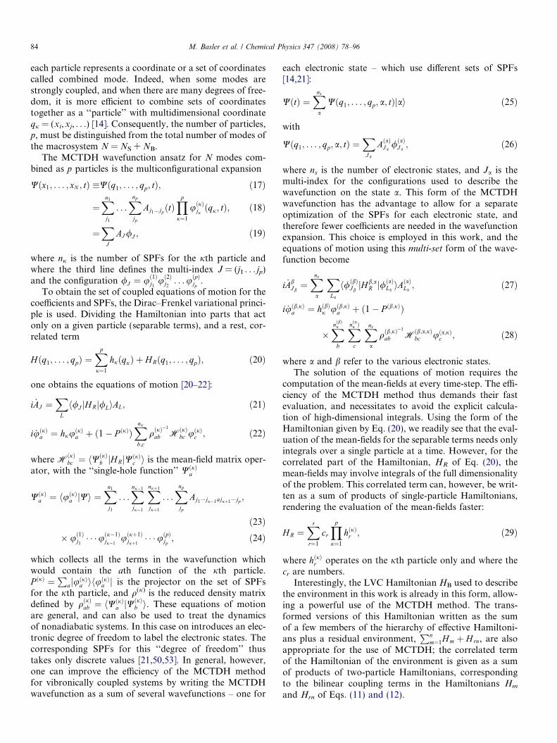
mg 0.258 �0.212 0.255mu 0.091 0.3181 0.2753 �0.0318 �0.03672 0.1508 �0.0782 �0.03253 0.1413 0.0445 �0.06934 0.1206 0.0583 0.07685 0.0980 0.0803 �0.06676 0.0828 0.0646 �0.07547 0.0732 0.0512 0.06768 0.0809 �0.04409 0.0716 �0.070410 0.0568 �0.032311 0.0539 �0.047812 0.0443 �0.0200 �0.0219 �0.020413 0.0400 �0.0110 0.0100 �0.015214 0.0358 �0.0156 �0.0155 �0.014715 0.0301 �0.0136 �0.0160 0.009916 0.0279 �0.0153 0.0166 �0.005217 0.0262 0.0142 �0.0123 �0.005518 0.0229 0.0155 �0.0100 �0.007419 0.0216 �0.0119 0.0141 �0.009820 0.0197 0.0113 0.0115 0.0081
The mode-label mg and mu represent the tuning and coupling modes of thesystem, respectively. The vertical energy split is E2 � E1 = 0.4 eV. Thesystem’s parameters are taken from Ref. [1]. The parameters for the modelenvironment are taken from Ref. [35].All values are given in eV.
Table 2Parameters of the first and second members of the hierarchy of effectiveHamiltonians, H1 and H2, for the first example
H1 Xi Kð1Þi Kð2Þi Ki
1 0.0644 0.0642 0.0241 0.99982 0.1002 0.6089 �0.8235 �0.00843 0.1274 �0.7907 �0.5667 0.0181�jð1Þ ¼ 0:1666 �jð2Þ ¼ 0:1728 �k ¼ 0:1074
H2 Xj d1j d2j d3j
4 0.0517 0.0139 0.0012 �0.00425 0.1002 �0.0008 �0.0287 0.01516 0.1846 �0.0014 0.0130 0.0587
All values are in eV.
86 M. Basler et al. / Chemical Physics 347 (2008) 78–96
aim to identify a suitable model system which features asystem part that is as small as possible: in particular, atwo-mode system giving rise to a CI. As an appropriatecase, we choose the 2-mode model derived to study thedynamics of the ground and first excited states of the but-atriene cation ðC4Hþ4 Þ [57,1]. This prototypical model com-prises one tuning mode and one coupling mode. Wemention that the quantum dynamics of the butatriene cat-ion in its full dimensionality (18 modes), using the second-order vibronic coupling model have been studied [23]. Ourapproach is designed for LVC environments, and, in thepresent study, the basic two-mode model is coupled to an– hypothetical – environment consisting of 20 modes. Theenvironment is a model determined by realistic choices ofthe parameters appearing in HB, Eq. (3), but is notexpected to simulate the neglected intramolecular modesof butatriene.
This example is similar to the first one discussed in Ref.[35]. In the latter reference, only the first member of thehierarchy of effective Hamiltonian was employed. We shallhere include additional members of the hierarchy and treatthe residual environment by TDH. All the calculations tobe reported in this work were carried out using the Heidel-berg Package of MCTDH [58].
For this example, each member of the hierarchy of effec-tive Hamiltonians is comprised of three effective modes.This corresponds to the most general situation of the effec-tive-mode formalism for two electronic states, and we shalldiscuss the results in details. The parameters of the 2-modesystem are taken from Refs. [57,1] and those of the envi-ronment from Ref. [35]. They are collected in Table 1.
In the following, we shall present results for six differentcases: (i) 2-mode system alone, (ii) system augmented bythe original environment treated by TDH, (iii) system plusone member of the hierarchy of effective Hamiltonians (3effective modes), (iv) system plus two members of the hier-archy (6 effective modes), and cases (v) and (vi) which aresimilar to cases (iii) and (iv), respectively, but augmentedby the corresponding residual environment treated by theTDH. All the results are compared to exact ones, obtainedby propagating the full multiconfigurational wavefunctionof the 22-mode system–environment complex. The para-meters corresponding to our various cases are collected inTables 1–3. The propagation time T is 100 fs, thus allowingto calculate autocorrelation functions up to 200 fs usingEq. (31).
In the following, to simplify the notation, we shallabbreviate effective mode by EM and the residual environ-ment treated with the TDH approximation by HRE – forHartree residual environment.
3.2.1. Autocorrelation function
Fig. 1 presents the absolute value of the autocorrelationfunctions for the six cases mentioned above, along with theexact one for comparison. An initial excitation to the upperelectronic state is considered. The figure is composed offour panels. Panel A shows the autocorrelation functions
for the system alone and the system plus the original envi-ronment treated with TDH. Panel B compares the use ofthe system plus 3 or 6 effective modes, neglecting the resid-ual environment. Panel C (D) presents the results for thesystem plus 3 (6) effective modes, augmented or not bythe 17 (14) residual modes treated with TDH. In all panelsthe exact result is shown for comparison. Pay attention tothe ordinate-scale which is chosen to emphasize the tail ofthe autocorrelation functions: for panel A, this scale ishowever 10 times larger than in the three other panels!Of course, at t = 0, the value of the autocorrelation func-tions is unity.
Let us first discuss panel A, showing the results for thesystem alone, the system plus TDH and the exact one.We see the very important impact of the environment.
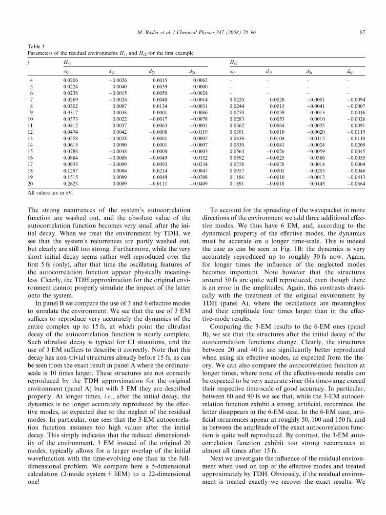
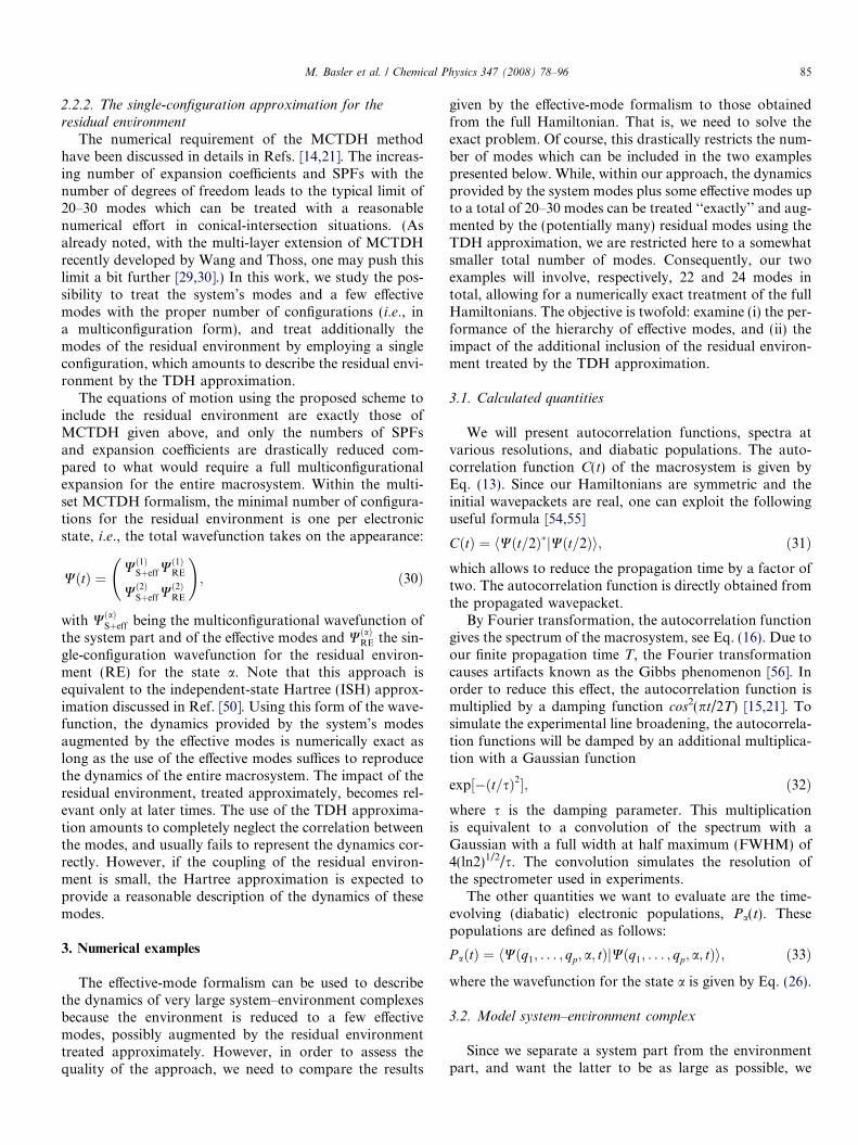
Table 3Parameters of the residual environments Hr1 and Hr2 for the first example
j Hr1 Hr2
xj d1j d2j d3j xj d4j d5j d6j
4 0.0206 �0.0026 0.0015 0.0062 – – – –5 0.0224 0.0040 0.0039 0.0000 – – – –6 0.0238 �0.0015 0.0050 �0.0024 – – – –7 0.0269 �0.0024 0.0040 �0.0014 0.0220 0.0020 �0.0001 �0.00948 0.0302 0.0007 0.0134 �0.0031 0.0244 0.0015 �0.0041 �0.00079 0.0317 �0.0038 0.0001 �0.0086 0.0250 0.0059 �0.0013 �0.0016
10 0.0373 0.0022 �0.0017 �0.0078 0.0283 0.0053 0.0010 �0.002611 0.0412 0.0037 0.0063 �0.0001 0.0362 0.0064 �0.0035 0.009112 0.0474 0.0042 �0.0008 �0.0119 0.0391 0.0010 �0.0020 �0.011913 0.0558 �0.0028 �0.0001 0.0005 0.0436 �0.0104 �0.0115 �0.011014 0.0615 0.0090 0.0001 �0.0007 0.0530 �0.0041 �0.0024 0.020915 0.0788 �0.0048 �0.0000 �0.0003 0.0564 �0.0026 �0.0059 0.004516 0.0884 �0.0008 �0.0049 0.0152 0.0592 �0.0025 0.0386 �0.005517 0.0933 �0.0009 0.0093 0.0234 0.0758 �0.0078 0.0014 0.000418 0.1297 0.0004 0.0214 �0.0047 0.0957 0.0001 �0.0205 �0.004619 0.1515 0.0009 0.0049 �0.0298 0.1186 �0.0010 �0.0012 �0.041320 0.2623 0.0009 �0.0111 �0.0409 0.1891 �0.0018 0.0145 �0.0664
All values are in eV.
M. Basler et al. / Chemical Physics 347 (2008) 78–96 87
The strong recurrences of the system’s autocorrelationfunction are washed out, and the absolute value of theautocorrelation function becomes very small after the ini-tial decay. When we treat the environment by TDH, wesee that the system’s recurrences are partly washed out,but clearly are still too strong. Furthermore, while the veryshort initial decay seems rather well reproduced over thefirst 5 fs (only), after that time the oscillating features ofthe autocorrelation function appear physically meaning-less. Clearly, the TDH approximation for the original envi-ronment cannot properly simulate the impact of the latteronto the system.
In panel B we compare the use of 3 and 6 effective modesto simulate the environment. We see that the use of 3 EMsuffices to reproduce very accurately the dynamics of theentire complex up to 15 fs, at which point the ultrafastdecay of the autocorrelation function is nearly complete.Such ultrafast decay is typical for CI situations, and theuse of 3 EM suffices to describe it correctly. Note that thisdecay has non-trivial structures already before 15 fs, as canbe seen from the exact result in panel A where the ordinate-scale is 10 times larger. These structures are not correctlyreproduced by the TDH approximation for the originalenvironment (panel A) but with 3 EM they are describedproperly. At longer times, i.e., after the initial decay, thedynamics is no longer accurately reproduced by the effec-tive modes, as expected due to the neglect of the residualmodes. In particular, one sees that the 3-EM autocorrela-tion function assumes too high values after the initialdecay. This simply indicates that the reduced dimensional-ity of the environment, 3 EM instead of the original 20modes, typically allows for a larger overlap of the initialwavefunction with the time-evolving one than in the full-dimensional problem. We compare here a 5-dimensionalcalculation (2-mode system + 3EM) to a 22-dimensionalone!
To account for the spreading of the wavepacket in moredirections of the environment we add three additional effec-tive modes. We thus have 6 EM, and, according to thedynamical property of the effective modes, the dynamicsmust be accurate on a longer time-scale. This is indeedthe case as can be seen in Fig. 1B: the dynamics is veryaccurately reproduced up to roughly 30 fs now. Again,for longer times the influence of the neglected modesbecomes important. Note however that the structuresaround 50 fs are quite well reproduced, even though thereis an error in the amplitudes. Again, this contrasts drasti-cally with the treatment of the original environment byTDH (panel A), where the oscillations are meaninglessand their amplitude four times larger than in the effec-tive-mode results.
Comparing the 3-EM results to the 6-EM ones (panelB), we see that the structures after the initial decay of theautocorrelation functions change. Clearly, the structuresbetween 20 and 40 fs are significantly better reproducedwhen using six effective modes, as expected from the the-ory. We can also compare the autocorrelation function atlonger times, where none of the effective-mode results canbe expected to be very accurate since this time-range exceedtheir respective time-scale of good accuracy. In particular,between 60 and 90 fs we see that, while the 3-EM autocor-relation function exhibit a strong, artificial, recurrence, thelatter disappears in the 6-EM case. In the 6-EM case, arti-ficial recurrences appear at roughly 50, 100 and 150 fs, andin between the amplitude of the exact autocorrelation func-tion is quite well reproduced. By contrast, the 3-EM auto-correlation function exhibit too strong recurrences atalmost all times after 15 fs.
Next we investigate the influence of the residual environ-ment when used on top of the effective modes and treatedapproximately by TDH. Obviously, if the residual environ-ment is treated exactly we recover the exact results. We
D
C
B
A
Fig. 1. Absolute value of the autocorrelation functions as a function oftime for the first example. The figure contains four panels. Note that theordinate-scale is ten times larger for panel A than for the other panels. Theline-coding is the same for all panels. (Red, in all panels) full line: exact 22-dimensional result. (Black, uppermost line in panel A) full line: systemalone. (Black, only in panel A) dashed line: system plus TDH approx-imation for all the original modes of the environment. (Green) long-dashed line: system plus 3 effective modes (EM). (Pink) dotted line: systemplus 6 EM. (Dark blue) short-dashed line: system plus 3 EM plus the 17-mode Hartree residual environment (HRE). (Light-blue) dashed-dottedline: system plus 6 EM plus 14-mode HRE. Panel A shows the result forthe system alone and the system plus the original environment treatedby TDH. Panel B compares the exact result to the one obtained with the
88 M. Basler et al. / Chemical Physics 347 (2008) 78–96
start by considering panel C of Fig. 1, which compares the3-EM results obtained with and without the Hartree resid-ual environment (HRE). We see that the improvement isindeed very good: the autocorrelation function with HREfollows correctly the exact one up to 80 fs. The results inthe time-range between 15 and 40 fs is particularly wellimproved. Importantly also, the artificial recurrence ofthe 3-EM result around 70 fs is washed out. The HRE,which allows for the wavefunction to spread into all direc-tions of the environment, but neglect all correlationsbetween the residual modes and the effective modes, pro-vides a clear improvement of the overall behavior of theautocorrelation function. When comparing the results for6EM and 6EM + HRE, panel D, similar conclusions hold.In particular, the intensity of the recurrence around 100 fsof the 6-EM result is significantly decreased and is now rea-sonably close to the exact one.
The action of the HRE is mainly to decrease the inten-sity of the (artificial) recurrences and improves the EMresults on the intermediate and long times. We want torecall that only the tail of the autocorrelation functionsare shown: the absolute error is indeed small in all effec-tive-mode cases. We turn now to the discussion of the spec-tra obtained by Fourier transform of the autocorrelationfunctions.
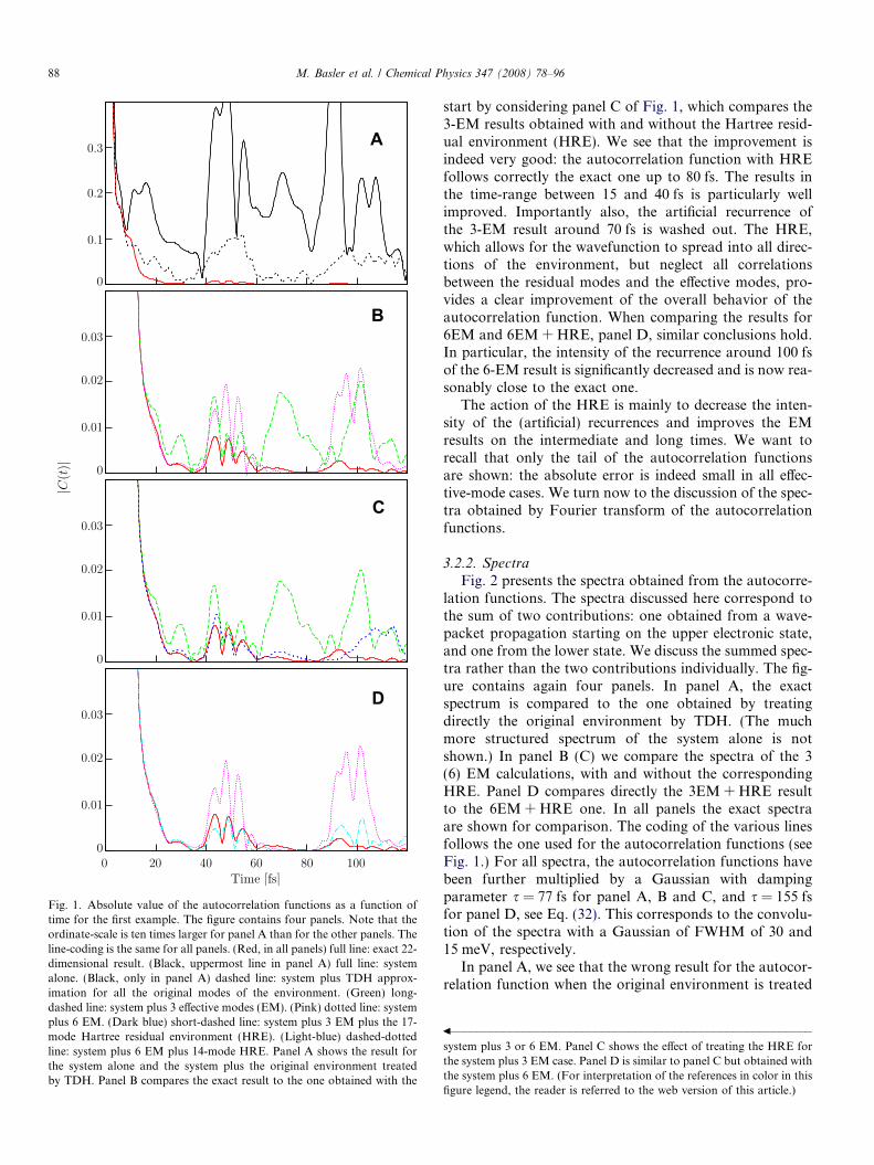
3.2.2. Spectra
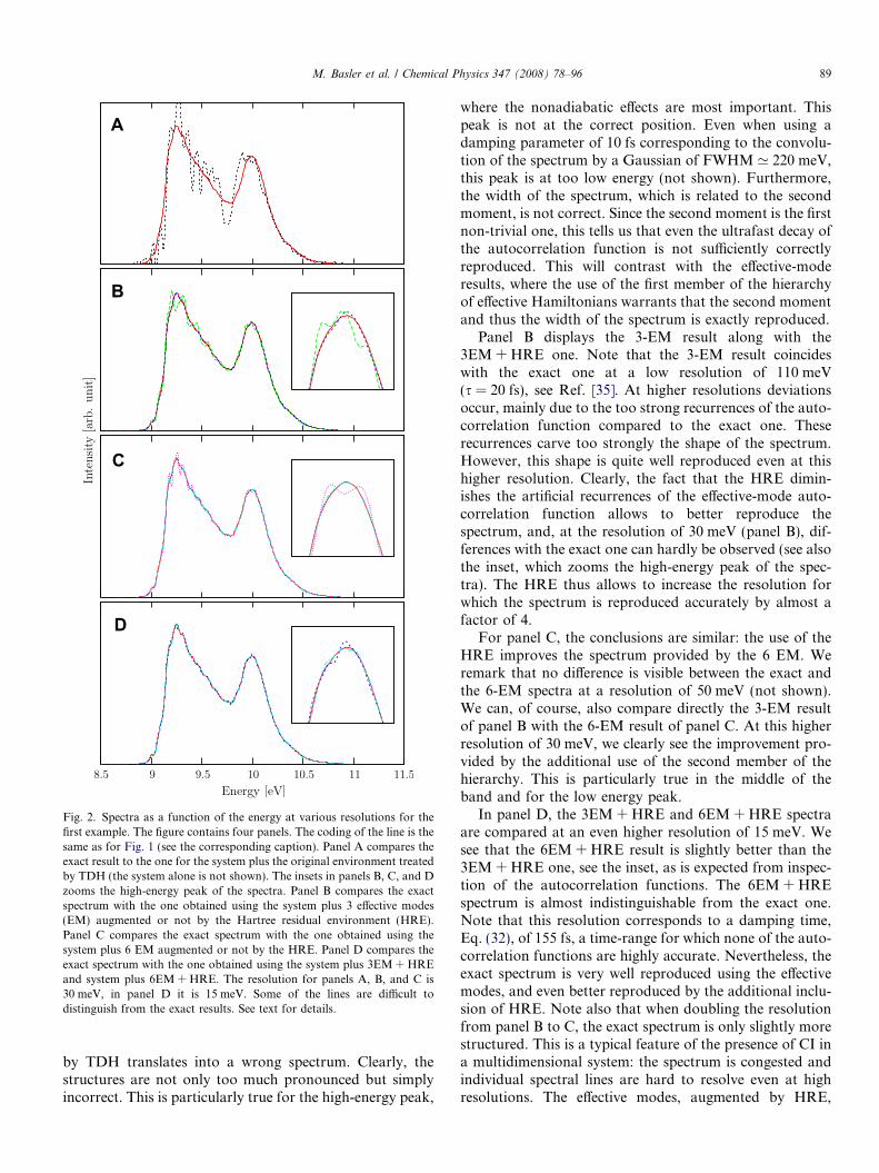
Fig. 2 presents the spectra obtained from the autocorre-lation functions. The spectra discussed here correspond tothe sum of two contributions: one obtained from a wave-packet propagation starting on the upper electronic state,and one from the lower state. We discuss the summed spec-tra rather than the two contributions individually. The fig-ure contains again four panels. In panel A, the exactspectrum is compared to the one obtained by treatingdirectly the original environment by TDH. (The muchmore structured spectrum of the system alone is notshown.) In panel B (C) we compare the spectra of the 3(6) EM calculations, with and without the correspondingHRE. Panel D compares directly the 3EM + HRE resultto the 6EM + HRE one. In all panels the exact spectraare shown for comparison. The coding of the various linesfollows the one used for the autocorrelation functions (seeFig. 1.) For all spectra, the autocorrelation functions havebeen further multiplied by a Gaussian with dampingparameter s = 77 fs for panel A, B and C, and s = 155 fsfor panel D, see Eq. (32). This corresponds to the convolu-tion of the spectra with a Gaussian of FWHM of 30 and15 meV, respectively.
In panel A, we see that the wrong result for the autocor-relation function when the original environment is treated
N ������������������������������������������������������system plus 3 or 6 EM. Panel C shows the effect of treating the HRE for
the system plus 3 EM case. Panel D is similar to panel C but obtained with
the system plus 6 EM. (For interpretation of the references in color in this
figure legend, the reader is referred to the web version of this article.)
A
B
C
D
Fig. 2. Spectra as a function of the energy at various resolutions for thefirst example. The figure contains four panels. The coding of the line is thesame as for Fig. 1 (see the corresponding caption). Panel A compares theexact result to the one for the system plus the original environment treatedby TDH (the system alone is not shown). The insets in panels B, C, and Dzooms the high-energy peak of the spectra. Panel B compares the exactspectrum with the one obtained using the system plus 3 effective modes(EM) augmented or not by the Hartree residual environment (HRE).Panel C compares the exact spectrum with the one obtained using thesystem plus 6 EM augmented or not by the HRE. Panel D compares theexact spectrum with the one obtained using the system plus 3EM + HREand system plus 6EM + HRE. The resolution for panels A, B, and C is30 meV, in panel D it is 15 meV. Some of the lines are difficult todistinguish from the exact results. See text for details.
M. Basler et al. / Chemical Physics 347 (2008) 78–96 89
by TDH translates into a wrong spectrum. Clearly, thestructures are not only too much pronounced but simplyincorrect. This is particularly true for the high-energy peak,
where the nonadiabatic effects are most important. Thispeak is not at the correct position. Even when using adamping parameter of 10 fs corresponding to the convolu-tion of the spectrum by a Gaussian of FWHM ’ 220 meV,this peak is at too low energy (not shown). Furthermore,the width of the spectrum, which is related to the secondmoment, is not correct. Since the second moment is the firstnon-trivial one, this tells us that even the ultrafast decay ofthe autocorrelation function is not sufficiently correctlyreproduced. This will contrast with the effective-moderesults, where the use of the first member of the hierarchyof effective Hamiltonians warrants that the second momentand thus the width of the spectrum is exactly reproduced.
Panel B displays the 3-EM result along with the3EM + HRE one. Note that the 3-EM result coincideswith the exact one at a low resolution of 110 meV(s = 20 fs), see Ref. [35]. At higher resolutions deviationsoccur, mainly due to the too strong recurrences of the auto-correlation function compared to the exact one. Theserecurrences carve too strongly the shape of the spectrum.However, this shape is quite well reproduced even at thishigher resolution. Clearly, the fact that the HRE dimin-ishes the artificial recurrences of the effective-mode auto-correlation function allows to better reproduce thespectrum, and, at the resolution of 30 meV (panel B), dif-ferences with the exact one can hardly be observed (see alsothe inset, which zooms the high-energy peak of the spec-tra). The HRE thus allows to increase the resolution forwhich the spectrum is reproduced accurately by almost afactor of 4.
For panel C, the conclusions are similar: the use of theHRE improves the spectrum provided by the 6 EM. Weremark that no difference is visible between the exact andthe 6-EM spectra at a resolution of 50 meV (not shown).We can, of course, also compare directly the 3-EM resultof panel B with the 6-EM result of panel C. At this higherresolution of 30 meV, we clearly see the improvement pro-vided by the additional use of the second member of thehierarchy. This is particularly true in the middle of theband and for the low energy peak.
In panel D, the 3EM + HRE and 6EM + HRE spectraare compared at an even higher resolution of 15 meV. Wesee that the 6EM + HRE result is slightly better than the3EM + HRE one, see the inset, as is expected from inspec-tion of the autocorrelation functions. The 6EM + HREspectrum is almost indistinguishable from the exact one.Note that this resolution corresponds to a damping time,Eq. (32), of 155 fs, a time-range for which none of the auto-correlation functions are highly accurate. Nevertheless, theexact spectrum is very well reproduced using the effectivemodes, and even better reproduced by the additional inclu-sion of HRE. Note also that when doubling the resolutionfrom panel B to C, the exact spectrum is only slightly morestructured. This is a typical feature of the presence of CI ina multidimensional system: the spectrum is congested andindividual spectral lines are hard to resolve even at highresolutions. The effective modes, augmented by HRE,
90 M. Basler et al. / Chemical Physics 347 (2008) 78–96
reproduce very well the spectral envelope in such situa-tions, while the direct use of TDH for the environmentfails.
3.2.3. Discussion
With this numerical example we see that the dynamics isaccurately reproduced on a short-time-scale by using onlythree effective modes to represent the environment. Thetime-range of accuracy is increased when three additionaleffective modes are used, corresponding to a truncationof the hierarchy of effective Hamiltonians at second order.These results are in complete accordance with the theoret-ical predictions [18,33,44].
Regarding the autocorrelation functions, the use of areduced number of effective modes leads to artificial recur-rences after the time-range of accuracy. This can be under-stood by considering the dimensionality of the problem:the neglect of the residual environment suppresses the pos-sibility for the nuclear motion to explore the full-dimen-sional space, resulting in an increased overlap betweenthe initial wavepacket and the time-evolving one. By allow-ing the macrosystem to explore the full space, even using anapproximate treatment for the residual environment, thisoverlap is decreased and the values of the autocorrelationfunctions become closer to the exact one over the wholetime-range studied. For this example, the neglected correla-tions between the residual modes seem not to play a crucialrole, and spectra with higher resolutions can be accuratelyobtained by using only one or two members of the hierar-chy of effective Hamiltonian augmented by the HRE – forinstance, from 110 meV to 30 meV when using three effec-tive modes and adding the HRE. Finally, we mention thatthe use of HRE also improves the electronic-state popula-tion dynamics provided by the effective modes over theentire time-range.
By contrast, TDH fails to represent properly the originalenvironment. This means that the correlation do play acrucial role for the original environment and cannot beneglected without strongly altering the quality of theresults. Using the effective-mode formalism, a relevant partof the correlation is properly accounted for, as well ascumulative effects of the full environment. The additionof the HRE is then of much better quality, and help toimprove the effective-mode results globally over the fulltime-range.
We make a last remark regarding the numerical require-ments. For this example, the exact calculation required3.8 Gbytes of memory, and, for comparison, the 6-EMone 250 Mbytes and the 6EM + HRE one 260 Mbytes.These values are obtained for calculations which satisfiedvery strict convergence criteria, because we wanted to beon safe grounds when comparing results with very smalldifferences. To add more modes to the full calculation willquickly requires a too large amount of memory, even whenusing MCTDH. In contrast, the effective modes are buildfrom all the modes of the environment, and can thus sim-ulate an arbitrarily large one. The effective coupling con-
stants will grow with the number of environmentalmodes, increasing accordingly the requirements for numer-ical convergence, but the number of effective modesremains the same avoiding the scaling problem. To addthe HRE on top of the effective modes adds a very moder-ate cost. Thus, the effective modes, augmented by the HRE,can be used to simulate the dynamics of macrosystems witha truly large number of modes.
3.3. S2 � S1 conical intersection in pyrazine: model
intramolecular environment
For our second example, we study the S2 � S1 conicalintersection of the pyrazine molecule, using a model intra-molecular environment. This model has been proposed byKrempl et al. [51] and is of very particular nature. The pyr-azine molecule is described by a 4-mode system [59–62],three tuning modes and one coupling mode, with parame-ters based on the multireference configuration interactioncalculations of Woywood et al. [63]. To represent theremaining intramolecular modes of the molecule – the envi-ronment – Krempl et al. added 20 harmonic-oscillatormodes with frequencies covering the range of the real pyr-azine ground-state normal modes [51,64]. This environ-ment consists in 20 tuning modes, with couplingconstants equal in modulus but opposite in sign for thetwo electronic states. The parameters of the 4-mode systemplus 20-mode environment are collected in Table 4. TheHamiltonian of the system is [51]
HS ¼X
s¼10a;6a;1;9a
xs
2ðp2
s þ x2s Þ1
þ�Dþ
Ps¼6a;1;9a
jð1Þs xs kx10a
kx10a DþP
s¼6a;1;9ajð2Þs xs
0B@
1CA ð34Þ
with the labelling of the modes following Ref. [65]. TheHamiltonian for the model NB = 20 modes environmentreads [51]
HB ¼XNB
i¼1
xi
2ðp2
i þ x2i Þ1þ
PNB
i¼1
jð1Þi xi 0
0PNB
i¼1
jð2Þi xi
0BBB@
1CCCA: ð35Þ
Note that, here, we have jð1Þi ¼ �jð2Þi for all environmentalmodes, see Table 4. For this particular form of the Hamil-tonian energy can flow to the environment only during achange of the diabatic state, i.e., if k = 0, system and envi-ronment are not coupled. This model system, or closely re-lated ones, have been widely used to study the pyrazine as abenchmark case for the impact of an intramolecular envi-ronment, see, for instance, Refs. [51,64,50,14,66–68]. InRef. [14], a full calculation treating all 24 modes withMCTDH is reported. This model has been also used tostudy, among others, the performance of the TDH approx-imation applied to an environment [50]. This is of interest
Table 5Parameters of the first four single-mode effective Hamiltonians for thepyrazine example
X1 0.3000 �j 0.1860X2 0.2060 d12 0.0710X3 0.2361 d23 0.0876X4 0.2164 d34 0.0900
All values are in eV.
Table 4Parameters of the original environment for the pyrazine example
Label xi jð1Þi jð2Þi
m10a 0.0935 – –m6a 0.0740 �0.0964 0.1194m1 0.1273 0.0470 0.2012m9a 0.1568 0.1594 0.04841 0.0400 0.0069 �0.00692 0.0589 0.0112 �0.01123 0.0778 0.0102 �0.01024 0.0968 0.0188 �0.01885 0.1157 0.0261 �0.02616 0.1347 0.0308 �0.03087 0.1536 0.0210 �0.02108 0.1726 0.0265 �0.02659 0.1915 0.0196 �0.019610 0.2105 0.0281 �0.028111 0.2294 0.0284 �0.028412 0.2484 0.0361 �0.036113 0.2673 0.0560 �0.056014 0.2863 0.0433 �0.043315 0.3052 0.0625 �0.062516 0.3242 0.0717 �0.071715 0.3431 0.0782 �0.078218 0.3621 0.0780 �0.078019 0.3810 0.0269 �0.026920 0.4000 0.0306 �0.0306
D = 0.4617 k = 0.1825
All values are in eV, and are taken from Krempl et al. [51]. The envi-ronmental modes (labelled by 1–20) are ordered in decreasing order ofcoupling strength.
M. Basler et al. / Chemical Physics 347 (2008) 78–96 91
for comparison with the present work. In fact, the conclu-sion of Ref. [50] is without appeal: TDH fails to correctlydescribe the dynamics provided by the environment. Wehave seen that this is also true for our former examplewhen TDH is used to treat the original environment. Here,the particular form of the coupling to the system, purelyelectronic, along with the very strong nonadiabaticity ofthe problem, explain why the correlation between themodes play a key role, and, in turn, why the TDH methodis not a good approximation for this problem. Indeed, theCI is located almost at the minimum of the upper surfaceand the spectrum is even stronger disturbed by the CI ascompared to the butatriene example. Consequently wecan view this example as a critical test for the TDHapproximation.
We aim here at studying whether TDH can neverthelessgive reasonable results when used on top of the effective-mode formalism or not. In addition, we shall investigatehow the effective modes alone, without HRE, perform.
Interestingly, the model environmental Hamiltonian ofEq. (35) corresponds to a particular case of the effective-mode formalism. While we generally need three effectivemodes to construct each member of the hierarchy of effec-tive Hamiltonians for a 2-state problem, like in the butatri-ene example, we need only one here. In Ref. [33], severalspecial cases of the formalism are detailed, including thisone, and we shall not give much details here. For the Ham-iltonian in consideration, only a single-effective-mode can
be identified, namely, X 1 ¼PNB
i¼1jð1Þi xi, because the inter-
state coupling of the environment is zero and the intrastatecouplings are symmetric, jð1Þi ¼ �jð2Þi . The procedure forconstructing the higher members of the hierarchy and thecorresponding residual environments is equivalent to thegeneral case presented in Ref. [43] and exposed in Section2.1.2. The first member of the hierarchy reads [33,36]
H 1 ¼X1
2ðP 2
1 þ X 21Þ1þ
�jX 1 0
0 ��jX 1
� �with �j given by Eq. (8). The higher members of the hierar-chy are described accordingly by a single-effective-modeand are given by (for m > 1)
Hm ¼Xm
2ðP 2
m þ X 2mÞ1þ dm�1;mðP m�1P m þ X m�1X mÞ1 ð36Þ
and the mth residual environment (including m = 1) isgiven by
Hrm ¼XNB
i¼mþ1
Xi
2ðP 2
i þ X 2i Þ1þ
XN B
i¼mþ1
dm;iðP mP i þ X mX iÞ1:
ð37ÞWe readily see that only H1 has a contribution which is notdiagonal in the electronic space and that the hierarchy re-duces here to a sequential coupling of single-effective-modes. As before, the residual environments contain allthe modes which are not included in the hierarchy. Notethat the single-effective-mode Hamiltonian H1 has alreadybeen used [36], and we are mainly concerned here withthe hierarchy and the addition of the HRE. The parametersof the first four members of the hierarchy of effective Ham-iltonians are presented in Table 5. Of course, the propertyregarding the moments discussed in Section 2.1.3 is pre-served for this particular case: each time we add a single-effective-mode, two more moments are exactly reproduced.Finally, we mention that calculations based on ab initio
data for all the 24 modes of the pyrazine molecule havebeen reported [15], but this study uses other parametersand implies a more involved Hamiltonian than the modeldiscussed here.
3.3.1. Analysis of the effective-mode results
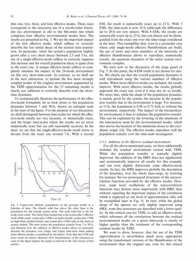
To illustrate the performance of the hierarchy of effec-tive modes in this particular situation of the effective-modeformalism, we present the time-evolving diabatic popula-tions of the upper, initially excited, electronic state, forthe five following cases: 4-mode system alone and system
92 M. Basler et al. / Chemical Physics 347 (2008) 78–96
plus one, two, three, and four effective modes. These casescorrespond to the successive use of a zeroth-order hierar-chy (no environment at all) to the 4th-order one whichcomprises four effective environmental modes here. Theresults are presented in Fig. 3. We see the important impactof the first effective mode, which suffices to correctlydescribe the fast initial decay of the excited state popula-tion. In particular, when the system’s population slightlygrows after a very short decay (between 2.5 and 5 fs), theuse of a single-effective-mode suffices to correctly suppressthis increase and the overall population decay is quite closeto the exact one. A unique effective mode suffices to com-pletely simulate the impact of the 24-mode environmenton this very short-time-scale. In contrast, as we shall seein the next subsection, to include the five most stronglycoupled modes of the original environment augmented bythe TDH approximation for the 15 remaining modes isclearly not sufficient to correctly describe even the short-time dynamics.
To systematically illustrate the performance of the effec-tive-mode formalism, let us look closer to the populationdynamics between 7 and 30 fs, shown on enlarged scalein the inset of the figure. For the purpose of our discussion,we shall distinguish between time-scales for which the effec-tive-mode results are very accurate, or numerically exact,and the larger time-scales where the results are no morenumerically exact but are still reasonably accurate. In theinset, we see that the single-effective-mode result starts todeviate from the exact one around 7 fs. With a second
Fig. 3. Upper-state diabatic populations of the pyrazine model as afunction of time. The (black) solid line above the other lines is thepopulation for the 4-mode system alone. The (red) solid line is the 24-mode exact result. The (dark-blue) dashed line is the system plus 1 effectivemode (EM) result; system plus 2 EM is in (pink) dotted, system plus 3 EMin (light-blue) dashed dotted, and system plus 4 EM (only in the inset) in(green) dashed. The inset zooms the population transfer from 7 to 30 fs,and illustrate how the addition of effective modes allows to accuratelydescribe the dynamics over longer and longer time-scale when addingmore effective modes, as predicted by the theory. Note that the 4 EM andexact result are almost identical. (For interpretation of the references incolor in this figure legend, the reader is referred to the web version of thisarticle.)
EM, the result is numerically exact up to 12 fs. With 3EMs, the time-scale is now 16 fs (although the differencesup to 20 fs are very minor). With 4 EMs, the results arenumerically exact up to 23 fs, but can almost not be distin-guished from the exact one over the time-range consideredin the inset. This exemplifies that, even in a particular casewhere only single-mode effective Hamiltonians are build,the use of more and more members of the hierarchy ofeffective Hamiltonians allows to reproduce, numericallyexactly, the quantum dynamics of the entire system–envi-ronment complex.
We turn now to the discussion of the large panel ofFig. 3. In this panel, the 4-EM result is not shown for clar-ity. We clearly see that the overall population dynamics iswell reproduced using the various numbers of effectivemodes. When more effective modes are included, the resultsimprove. With more effective modes, the results globallyapproach the exact one, even if it may not do so locally.We stress that, while the shape of the population dynamicsis mainly given by the system, the increase in the popula-tion transfer due to the environment is large. For instance,at 15 fs, the population is 0.48 or 0.75 with or without theenvironment, respectively. The impact of the intramolecu-lar environment is thus to enhance the population transfer.This can be explained by the lowering of the minimum ofthe intersection seam by the environmental modes, whichalso moves the location of this minimum closer to the coor-dinate origin [14]. The effective modes reproduce well thepopulation transfer over the time-scale investigated.
3.3.2. Addition of the Hartree residual environment
For all the above-mentioned cases, we have additionallyincluded the residual environment treated with TDH.While the population transfer is typically slightlyimproved, the addition of the HRE does not significantlyand systematically improve all results for this example,and can even slightly deteriorate some effective-moderesults. In fact, the HRE improves globally the descriptionof the dynamics, over the whole time-range, by loweringfor instance the too pronounced structures of the autocor-relation functions provided by the effective modes. How-ever, some local oscillations of the autocorrelationfunctions may deviate more importantly with HRE thanwithout, signaling the important impact of the correlationwhich is neglected at our level of approximation (this willbe exemplified later in Fig. 5). In turn, while the globalshape of the spectra are only slightly improved usingHRE, some fine structures are described with a lower qual-ity. In this critical case for TDH, to add an effective modewhich subsumes all the correlations between the residualenvironmental modes on a given time-scale is clearly ofhigher quality than the treatment of the correspondingresidual modes by TDH.
We want to show, however, that the use of the TDHapproximation is nevertheless much more appropriateusing the transformed versions of the Hamiltonian of theenvironment than the original one, even for this critical
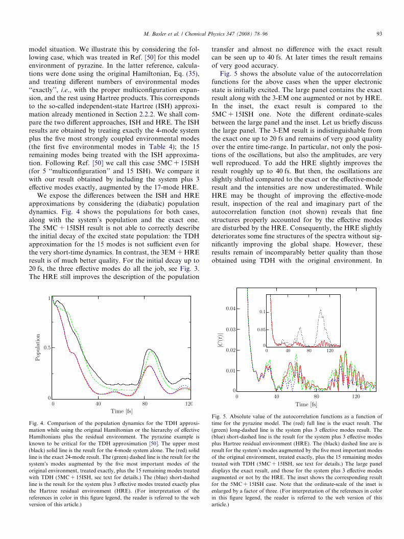
M. Basler et al. / Chemical Physics 347 (2008) 78–96 93
model situation. We illustrate this by considering the fol-lowing case, which was treated in Ref. [50] for this modelenvironment of pyrazine. In the latter reference, calcula-tions were done using the original Hamiltonian, Eq. (35),and treating different numbers of environmental modes‘‘exactly’’, i.e., with the proper multiconfiguration expan-sion, and the rest using Hartree products. This correspondsto the so-called independent-state Hartree (ISH) approxi-mation already mentioned in Section 2.2.2. We shall com-pare the two different approaches, ISH and HRE. The ISHresults are obtained by treating exactly the 4-mode systemplus the five most strongly coupled environmental modes(the first five environmental modes in Table 4); the 15remaining modes being treated with the ISH approxima-tion. Following Ref. [50] we call this case 5MC + 15ISH(for 5 ‘‘multiconfiguration’’ and 15 ISH). We compare itwith our result obtained by including the system plus 3effective modes exactly, augmented by the 17-mode HRE.
We expose the differences between the ISH and HREapproximations by considering the (diabatic) populationdynamics. Fig. 4 shows the populations for both cases,along with the system’s population and the exact one.The 5MC + 15ISH result is not able to correctly describethe initial decay of the excited state population: the TDHapproximation for the 15 modes is not sufficient even forthe very short-time dynamics. In contrast, the 3EM + HREresult is of much better quality. For the initial decay up to20 fs, the three effective modes do all the job, see Fig. 3.The HRE still improves the description of the population
Fig. 4. Comparison of the population dynamics for the TDH approxi-mation while using the original Hamiltonian or the hierarchy of effectiveHamiltonians plus the residual environment. The pyrazine example isknown to be critical for the TDH approximation [50]. The upper most(black) solid line is the result for the 4-mode system alone. The (red) solidline is the exact 24-mode result. The (green) dashed line is the result for thesystem’s modes augmented by the five most important modes of theoriginal environment, treated exactly, plus the 15 remaining modes treatedwith TDH (5MC + 15ISH, see text for details.) The (blue) short-dashedline is the result for the system plus 3 effective modes treated exactly plusthe Hartree residual environment (HRE). (For interpretation of thereferences in color in this figure legend, the reader is referred to the webversion of this article.)
transfer and almost no difference with the exact resultcan be seen up to 40 fs. At later times the result remainsof very good accuracy.
Fig. 5 shows the absolute value of the autocorrelationfunctions for the above cases when the upper electronicstate is initially excited. The large panel contains the exactresult along with the 3-EM one augmented or not by HRE.In the inset, the exact result is compared to the5MC + 15ISH one. Note the different ordinate-scalesbetween the large panel and the inset. Let us briefly discussthe large panel. The 3-EM result is indistinguishable fromthe exact one up to 20 fs and remains of very good qualityover the entire time-range. In particular, not only the posi-tions of the oscillations, but also the amplitudes, are verywell reproduced. To add the HRE slightly improves theresult roughly up to 40 fs. But then, the oscillations areslightly shifted compared to the exact or the effective-moderesult and the intensities are now underestimated. WhileHRE may be thought of improving the effective-moderesult, inspection of the real and imaginary part of theautocorrelation function (not shown) reveals that finestructures properly accounted for by the effective modesare disturbed by the HRE. Consequently, the HRE slightlydeteriorates some fine structures of the spectra without sig-nificantly improving the global shape. However, theseresults remain of incomparably better quality than thoseobtained using TDH with the original environment. In
Fig. 5. Absolute value of the autocorrelation functions as a function oftime for the pyrazine model. The (red) full line is the exact result. The(green) long-dashed line is the system plus 3 effective modes result. The(blue) short-dashed line is the result for the system plus 3 effective modesplus Hartree residual environment (HRE). The (black) dashed line are isresult for the system’s modes augmented by the five most important modesof the original environment, treated exactly, plus the 15 remaining modestreated with TDH (5MC + 15ISH, see text for details.) The large paneldisplays the exact result, and those for the system plus 3 effective modesaugmented or not by the HRE. The inset shows the corresponding resultfor the 5MC + 15ISH case. Note that the ordinate-scale of the inset isenlarged by a factor of three. (For interpretation of the references in colorin this figure legend, the reader is referred to the web version of thisarticle.)
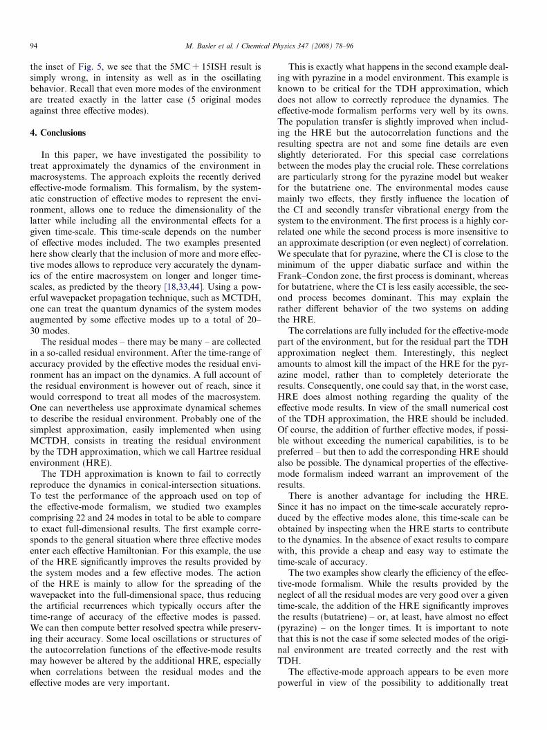
94 M. Basler et al. / Chemical Physics 347 (2008) 78–96
the inset of Fig. 5, we see that the 5MC + 15ISH result issimply wrong, in intensity as well as in the oscillatingbehavior. Recall that even more modes of the environmentare treated exactly in the latter case (5 original modesagainst three effective modes).
4. Conclusions
In this paper, we have investigated the possibility totreat approximately the dynamics of the environment inmacrosystems. The approach exploits the recently derivedeffective-mode formalism. This formalism, by the system-atic construction of effective modes to represent the envi-ronment, allows one to reduce the dimensionality of thelatter while including all the environmental effects for agiven time-scale. This time-scale depends on the numberof effective modes included. The two examples presentedhere show clearly that the inclusion of more and more effec-tive modes allows to reproduce very accurately the dynam-ics of the entire macrosystem on longer and longer time-scales, as predicted by the theory [18,33,44]. Using a pow-erful wavepacket propagation technique, such as MCTDH,one can treat the quantum dynamics of the system modesaugmented by some effective modes up to a total of 20–30 modes.
The residual modes – there may be many – are collectedin a so-called residual environment. After the time-range ofaccuracy provided by the effective modes the residual envi-ronment has an impact on the dynamics. A full account ofthe residual environment is however out of reach, since itwould correspond to treat all modes of the macrosystem.One can nevertheless use approximate dynamical schemesto describe the residual environment. Probably one of thesimplest approximation, easily implemented when usingMCTDH, consists in treating the residual environmentby the TDH approximation, which we call Hartree residualenvironment (HRE).
The TDH approximation is known to fail to correctlyreproduce the dynamics in conical-intersection situations.To test the performance of the approach used on top ofthe effective-mode formalism, we studied two examplescomprising 22 and 24 modes in total to be able to compareto exact full-dimensional results. The first example corre-sponds to the general situation where three effective modesenter each effective Hamiltonian. For this example, the useof the HRE significantly improves the results provided bythe system modes and a few effective modes. The actionof the HRE is mainly to allow for the spreading of thewavepacket into the full-dimensional space, thus reducingthe artificial recurrences which typically occurs after thetime-range of accuracy of the effective modes is passed.We can then compute better resolved spectra while preserv-ing their accuracy. Some local oscillations or structures ofthe autocorrelation functions of the effective-mode resultsmay however be altered by the additional HRE, especiallywhen correlations between the residual modes and theeffective modes are very important.
This is exactly what happens in the second example deal-ing with pyrazine in a model environment. This example isknown to be critical for the TDH approximation, whichdoes not allow to correctly reproduce the dynamics. Theeffective-mode formalism performs very well by its owns.The population transfer is slightly improved when includ-ing the HRE but the autocorrelation functions and theresulting spectra are not and some fine details are evenslightly deteriorated. For this special case correlationsbetween the modes play the crucial role. These correlationsare particularly strong for the pyrazine model but weakerfor the butatriene one. The environmental modes causemainly two effects, they firstly influence the location ofthe CI and secondly transfer vibrational energy from thesystem to the environment. The first process is a highly cor-related one while the second process is more insensitive toan approximate description (or even neglect) of correlation.We speculate that for pyrazine, where the CI is close to theminimum of the upper diabatic surface and within theFrank–Condon zone, the first process is dominant, whereasfor butatriene, where the CI is less easily accessible, the sec-ond process becomes dominant. This may explain therather different behavior of the two systems on addingthe HRE.
The correlations are fully included for the effective-modepart of the environment, but for the residual part the TDHapproximation neglect them. Interestingly, this neglectamounts to almost kill the impact of the HRE for the pyr-azine model, rather than to completely deteriorate theresults. Consequently, one could say that, in the worst case,HRE does almost nothing regarding the quality of theeffective mode results. In view of the small numerical costof the TDH approximation, the HRE should be included.Of course, the addition of further effective modes, if possi-ble without exceeding the numerical capabilities, is to bepreferred – but then to add the corresponding HRE shouldalso be possible. The dynamical properties of the effective-mode formalism indeed warrant an improvement of theresults.
There is another advantage for including the HRE.Since it has no impact on the time-scale accurately repro-duced by the effective modes alone, this time-scale can beobtained by inspecting when the HRE starts to contributeto the dynamics. In the absence of exact results to comparewith, this provide a cheap and easy way to estimate thetime-scale of accuracy.
The two examples show clearly the efficiency of the effec-tive-mode formalism. While the results provided by theneglect of all the residual modes are very good over a giventime-scale, the addition of the HRE significantly improvesthe results (butatriene) – or, at least, have almost no effect(pyrazine) – on the longer times. It is important to notethat this is not the case if some selected modes of the origi-nal environment are treated correctly and the rest withTDH.
The effective-mode approach appears to be even morepowerful in view of the possibility to additionally treat
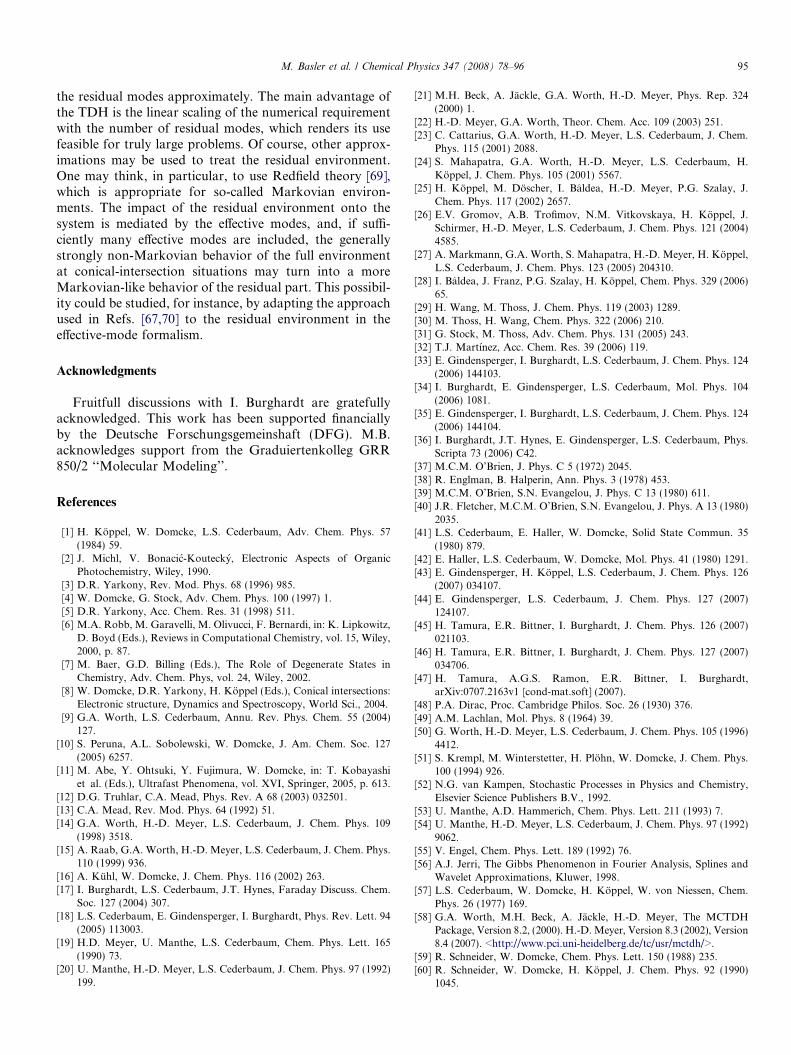
M. Basler et al. / Chemical Physics 347 (2008) 78–96 95
the residual modes approximately. The main advantage ofthe TDH is the linear scaling of the numerical requirementwith the number of residual modes, which renders its usefeasible for truly large problems. Of course, other approx-imations may be used to treat the residual environment.One may think, in particular, to use Redfield theory [69],which is appropriate for so-called Markovian environ-ments. The impact of the residual environment onto thesystem is mediated by the effective modes, and, if suffi-ciently many effective modes are included, the generallystrongly non-Markovian behavior of the full environmentat conical-intersection situations may turn into a moreMarkovian-like behavior of the residual part. This possibil-ity could be studied, for instance, by adapting the approachused in Refs. [67,70] to the residual environment in theeffective-mode formalism.
Acknowledgments
Fruitfull discussions with I. Burghardt are gratefullyacknowledged. This work has been supported financiallyby the Deutsche Forschungsgemeinshaft (DFG). M.B.acknowledges support from the Graduiertenkolleg GRR850/2 ‘‘Molecular Modeling’’.
References
[1] H. Koppel, W. Domcke, L.S. Cederbaum, Adv. Chem. Phys. 57(1984) 59.
[2] J. Michl, V. Bonacic-Koutecky, Electronic Aspects of OrganicPhotochemistry, Wiley, 1990.
[3] D.R. Yarkony, Rev. Mod. Phys. 68 (1996) 985.[4] W. Domcke, G. Stock, Adv. Chem. Phys. 100 (1997) 1.[5] D.R. Yarkony, Acc. Chem. Res. 31 (1998) 511.[6] M.A. Robb, M. Garavelli, M. Olivucci, F. Bernardi, in: K. Lipkowitz,
D. Boyd (Eds.), Reviews in Computational Chemistry, vol. 15, Wiley,2000, p. 87.
[7] M. Baer, G.D. Billing (Eds.), The Role of Degenerate States inChemistry, Adv. Chem. Phys, vol. 24, Wiley, 2002.
[8] W. Domcke, D.R. Yarkony, H. Koppel (Eds.), Conical intersections:Electronic structure, Dynamics and Spectroscopy, World Sci., 2004.
[9] G.A. Worth, L.S. Cederbaum, Annu. Rev. Phys. Chem. 55 (2004)127.
[10] S. Peruna, A.L. Sobolewski, W. Domcke, J. Am. Chem. Soc. 127(2005) 6257.
[11] M. Abe, Y. Ohtsuki, Y. Fujimura, W. Domcke, in: T. Kobayashiet al. (Eds.), Ultrafast Phenomena, vol. XVI, Springer, 2005, p. 613.
[12] D.G. Truhlar, C.A. Mead, Phys. Rev. A 68 (2003) 032501.[13] C.A. Mead, Rev. Mod. Phys. 64 (1992) 51.[14] G.A. Worth, H.-D. Meyer, L.S. Cederbaum, J. Chem. Phys. 109
(1998) 3518.[15] A. Raab, G.A. Worth, H.-D. Meyer, L.S. Cederbaum, J. Chem. Phys.
110 (1999) 936.[16] A. Kuhl, W. Domcke, J. Chem. Phys. 116 (2002) 263.[17] I. Burghardt, L.S. Cederbaum, J.T. Hynes, Faraday Discuss. Chem.
Soc. 127 (2004) 307.[18] L.S. Cederbaum, E. Gindensperger, I. Burghardt, Phys. Rev. Lett. 94
(2005) 113003.[19] H.D. Meyer, U. Manthe, L.S. Cederbaum, Chem. Phys. Lett. 165
(1990) 73.[20] U. Manthe, H.-D. Meyer, L.S. Cederbaum, J. Chem. Phys. 97 (1992)
199.
[21] M.H. Beck, A. Jackle, G.A. Worth, H.-D. Meyer, Phys. Rep. 324(2000) 1.
[22] H.-D. Meyer, G.A. Worth, Theor. Chem. Acc. 109 (2003) 251.[23] C. Cattarius, G.A. Worth, H.-D. Meyer, L.S. Cederbaum, J. Chem.
Phys. 115 (2001) 2088.[24] S. Mahapatra, G.A. Worth, H.-D. Meyer, L.S. Cederbaum, H.
Koppel, J. Chem. Phys. 105 (2001) 5567.[25] H. Koppel, M. Doscher, I. Baldea, H.-D. Meyer, P.G. Szalay, J.
Chem. Phys. 117 (2002) 2657.[26] E.V. Gromov, A.B. Trofimov, N.M. Vitkovskaya, H. Koppel, J.
Schirmer, H.-D. Meyer, L.S. Cederbaum, J. Chem. Phys. 121 (2004)4585.
[27] A. Markmann, G.A. Worth, S. Mahapatra, H.-D. Meyer, H. Koppel,L.S. Cederbaum, J. Chem. Phys. 123 (2005) 204310.
[28] I. Baldea, J. Franz, P.G. Szalay, H. Koppel, Chem. Phys. 329 (2006)65.
[29] H. Wang, M. Thoss, J. Chem. Phys. 119 (2003) 1289.[30] M. Thoss, H. Wang, Chem. Phys. 322 (2006) 210.[31] G. Stock, M. Thoss, Adv. Chem. Phys. 131 (2005) 243.[32] T.J. Martınez, Acc. Chem. Res. 39 (2006) 119.[33] E. Gindensperger, I. Burghardt, L.S. Cederbaum, J. Chem. Phys. 124
(2006) 144103.[34] I. Burghardt, E. Gindensperger, L.S. Cederbaum, Mol. Phys. 104
(2006) 1081.[35] E. Gindensperger, I. Burghardt, L.S. Cederbaum, J. Chem. Phys. 124
(2006) 144104.[36] I. Burghardt, J.T. Hynes, E. Gindensperger, L.S. Cederbaum, Phys.
Scripta 73 (2006) C42.[37] M.C.M. O’Brien, J. Phys. C 5 (1972) 2045.[38] R. Englman, B. Halperin, Ann. Phys. 3 (1978) 453.[39] M.C.M. O’Brien, S.N. Evangelou, J. Phys. C 13 (1980) 611.[40] J.R. Fletcher, M.C.M. O’Brien, S.N. Evangelou, J. Phys. A 13 (1980)
2035.[41] L.S. Cederbaum, E. Haller, W. Domcke, Solid State Commun. 35
(1980) 879.[42] E. Haller, L.S. Cederbaum, W. Domcke, Mol. Phys. 41 (1980) 1291.[43] E. Gindensperger, H. Koppel, L.S. Cederbaum, J. Chem. Phys. 126
(2007) 034107.[44] E. Gindensperger, L.S. Cederbaum, J. Chem. Phys. 127 (2007)
124107.[45] H. Tamura, E.R. Bittner, I. Burghardt, J. Chem. Phys. 126 (2007)
021103.[46] H. Tamura, E.R. Bittner, I. Burghardt, J. Chem. Phys. 127 (2007)
034706.[47] H. Tamura, A.G.S. Ramon, E.R. Bittner, I. Burghardt,
arXiv:0707.2163v1 [cond-mat.soft] (2007).[48] P.A. Dirac, Proc. Cambridge Philos. Soc. 26 (1930) 376.[49] A.M. Lachlan, Mol. Phys. 8 (1964) 39.[50] G. Worth, H.-D. Meyer, L.S. Cederbaum, J. Chem. Phys. 105 (1996)
4412.[51] S. Krempl, M. Winterstetter, H. Plohn, W. Domcke, J. Chem. Phys.
100 (1994) 926.[52] N.G. van Kampen, Stochastic Processes in Physics and Chemistry,
Elsevier Science Publishers B.V., 1992.[53] U. Manthe, A.D. Hammerich, Chem. Phys. Lett. 211 (1993) 7.[54] U. Manthe, H.-D. Meyer, L.S. Cederbaum, J. Chem. Phys. 97 (1992)
9062.[55] V. Engel, Chem. Phys. Lett. 189 (1992) 76.[56] A.J. Jerri, The Gibbs Phenomenon in Fourier Analysis, Splines and
Wavelet Approximations, Kluwer, 1998.[57] L.S. Cederbaum, W. Domcke, H. Koppel, W. von Niessen, Chem.
Phys. 26 (1977) 169.[58] G.A. Worth, M.H. Beck, A. Jackle, H.-D. Meyer, The MCTDH
Package, Version 8.2, (2000). H.-D. Meyer, Version 8.3 (2002), Version8.4 (2007). <http://www.pci.uni-heidelberg.de/tc/usr/mctdh/>.
[59] R. Schneider, W. Domcke, Chem. Phys. Lett. 150 (1988) 235.[60] R. Schneider, W. Domcke, H. Koppel, J. Chem. Phys. 92 (1990)
1045.

96 M. Basler et al. / Chemical Physics 347 (2008) 78–96
[61] G. Stock, W. Domcke, J. Chem. Phys. 93 (1990) 5496.[62] R. Schneider, G. Stock, A.L. Sobolewsky, W. Domcke, J. Chem.
Phys. 96 (1992) 5298.[63] C. Woywood, W. Domcke, A.L. Sobolewsky, H.-J. Werner, J. Chem.
Phys. 100 (1994) 1400.[64] S. Krempl, M. Winterstetter, W. Domcke, J. Chem. Phys. 102 (1995)
926.
[65] K.K. Innes, I.G. Ross, W.R. Monaw, J. Mol. Spectrosc. 132 (1988) 492.[66] B. Wolfseder, W. Domcke, Chem. Phys. Lett. 235 (1995) 370.[67] A. Kuhl, W. Domcke, J. Chem. Phys. 116 (2002) 263.[68] I. Burghardt, H. Tamura, in: K.H. Hughes (Ed.), Dynamics of Open
Quantum Systems, CCP6, 2006.[69] A.G. Redfield, Adv. Magn. Reson. 1 (1965) 1.[70] D. Egorova, W. Domcke, Chem. Phys. Lett. 384 (2004) 157.