Kharosti inscriptions discovered by Sir Aurel Stein in Chinese ...
Upload
independentCategory
view
3download
0
arX
iv:1
003.
6039
v2 [
mat
h.PR
] 2
6 O
ct 2
010
STEIN COUPLINGS FOR NORMAL APPROXIMATION
LOUIS H. Y. CHEN AND ADRIAN ROLLIN
Abstract. In this article we propose a general framework for normalapproximation using Stein’s method. We introduce the new concept ofStein couplings and we show that it lies at the heart of popular ap-proaches such as the local approach, exchangeable pairs, size biasingand many other approaches. We prove several theorems with whichnormal approximation for the Wasserstein and Kolmogorov metrics be-comes routine once a Stein coupling is found. To illustrate the versa-tility of our framework we give applications in Hoeffding’s combinato-rial central limit theorem, functionals in the classic occupancy scheme,neighbourhood statistics of point patterns with fixed number of pointsand functionals of the components of randomly chosen vertices of sub-critical Erdos-Renyi random graphs. In all these cases, we use new,non-standard couplings.
Contents
1. Introduction 21.1. A short introduction to Stein’s method 31.2. An outline of our approach 51.3. The probability metrics 92. Main results 102.1. Wasserstein distance 112.2. Kolmogorov distance 123. Couplings 163.1. Exchangeable pairs and extensions 173.2. Local dependence and related couplings 223.3. Size-biasing 253.4. Interpolation to independence 253.5. Local symmetry 273.6. Abstract approaches 274. Applications 284.1. Hoeffding’s combinatorial statistic 284.2. Functionals in the classic occupancy scheme 304.3. Neighbourhood statistics of a fixed number of uniformly distributed
points 344.4. Susceptibility and related statistics in the sub-critical Erdos-Renyi
random graph 385. Zero bias transformation 436. Proofs of main results 456.1. Preliminaries 456.2. Bound on the Wasserstein distance 466.3. Bounds on the Kolmogorov distance 46Acknowledgments 51References 51
Version from October 27, 2010, 00:20.
1

STEIN COUPLINGS FOR NORMAL APPROXIMATION 2
1. Introduction
Since its introduction in the early 70s, Stein’s method has gone througha vivid development. First used by Stein (1972) for normal approximationof m-dependent sequences, it was gradually modified and generalized toother distributions and different dependency settings. Among the few im-portant contributions that influenced the theoretical understanding of themethod is the book by Stein (1986), where the concepts of auxiliary ran-domization and exchangeable pairs are introduced. Another corner stoneis the generator method, independently introduced by Barbour (1988) andGotze (1991), which allows for an adaptation of the method to more com-plicated approximating distributions, such as compound Poisson distribu-tion, Poisson point processes and Gaussian diffusions. Diaconis and Zabell(1991) give a connection between Stein’s method and orthogonal polynomi-als; see also Goldstein and Reinert (2005a), who related this approach todistributional transformations. A more recent development was initiated byNourdin and Peccati (2009) and related articles, where a fruitful theory fornormal approximation for functionals of Gaussian measures, Rademachersequences and Poisson measures is developed. Despite these achievements,relatively little effort has been put into building up a rigorous theoreticalframework for the method in order to unify and generalize the variety ofknown results.
In particular for normal approximation, a wide range of different ap-proaches has appeared over the last decades. Among the most prominent ap-proaches are the local approach, dating back to Stein (1972) and extensivelystudied by Chen and Shao (2004), the exchangeable pairs approach by Stein(1986), further developed by Rinott and Rotar′ (1997), Rollin (2007b) andRollin (2008a) with a variety of applications such as weighted U -statistics,anti-voter model on finite graphs and models in statistical mechanics, andthe size and zero bias couplings by Goldstein and Rinott (1996) and Goldstein and Reinert(1997), respectively. Another approach was introduced by Chatterjee (2008)for functionals of independent random variables (we will discuss a moregeneral version of this approach—called interpolation to independence—in Section 3.4). In addition to these abstract approaches, many otherad-hoc constructions have been used to tackle specific problems, such asHo and Chen (1978) and Bolthausen (1984) for the combinatorial limit the-orem, Barbour, Karonski, and Rucinski (1989) and Rollin (2008b) for re-fined versions of local dependence and Barbour and Eagleson (1986) andZhao, Bai, Chao, and Liang (1997) for double indexed permutation statis-tics. However, despite all these achievements, a unifying framework is stillmissing and connections between the different approaches given in the lit-erature are vague, at best. Although making an attempt to systemati-cally discuss Stein’s method, survey articles such as Reinert (1998) andRinott and Rotar′ (2000) illustrate the key issue here: for each approach aseparate theorem is proved, and then typically only for one specific metric.
The reason for this seems to be the following. For all of these approaches,the involved random variables either have to satisfy some more or less ab-stract conditions or some specific properties in the dependence structure areexploited to obtain the results. This could be a defining equation like in the

STEIN COUPLINGS FOR NORMAL APPROXIMATION 3
size-biasing approach, a linearity assumption on a conditional expectationfor exchangeable pairs, a local dependence structure, or other propertiesand conditions. Depending on the specific form of these conditions, thequantities arising from using Stein’s method—seemingly—have to be han-deled differently. Although in simpler applications it might be clear how todirectly manipulate these expressions in an ad-hoc way in order to success-fully apply Stein’s method, this is less feasible for more complex situations.Chatterjee (2008) proposes an approach for functionals of finite collectionsof independent random variables. His approach comes at the cost of a rathercomplicated bound, and for many applications optimal results (in terms ofmoment conditions and metrics) may not be obtained that way (c.f. thedifference between Corollaries 2.2 and 2.3 below). It is crucial to exploitproperties of the random variables at hand in order to express the errorbounds in terms of simple and manageable expressions. To achieve this, wewill explore what the abstract key conditions are that allow for a success-ful implementation of Stein’s method for normal approximation—a questionthat has not yet been addressed in the literature. Our framework providessuch a set of conditions along with a variety of “plug-in” type theorems.Not only does our framework show the connection between all the abovementioned approaches, but it also introduces some crucial generalisationsand hence flexibility into Stein’s method for normal approximation.
Our main tool is that of couplings; more specifically, we introduce the newconcept of Stein couplings. We provide general approximation theorems withrespect to the Wasserstein and Kolmogorov metrics, where the error termsare expressed in terms of the relationship between the involved coupled ran-dom variables. Although we relate the different known approaches via Steincouplings, our applications also show that the distinction usually made be-tween these approaches is rather artificial. Most of the couplings used in ourapplications cannot be clearly assigned to one of the known approaches, butemerge naturally from the problem at hand and are therefore constructed ina more ad-hoc way. Nevertheless, in Section 3 we make an attempt to givea systematic overview over the different coupling constructions, being verywell aware of the fact that other ways of classifying these couplings may beequally reasonable.
1.1. A short introduction to Stein’s method. We assume throughoutthis article that W is a random variable whose distribution is to be approx-imated by a standard normal distribution and we also assume that W hasfinite variance. Stein’s method for normal approximation is based on thefact that, for all, say, Lipschitz continuous function f we haveEZf(Z) = Ef ′(Z) (1.1) 1
if and only if Z ∼ N(0, 1). Now, if it is the case thatEWf(W ) ≈ Ef ′(W ) (1.2) 2
for many functions f , we would expect that W is close to the normal distri-bution. With Stein’s method we can make this heuristic idea rigorous in thefollowing sense. Assume that, in order to measure the closeness of L (W )

STEIN COUPLINGS FOR NORMAL APPROXIMATION 4
and L (Z), we would like to boundEh(W )−Eh(Z) (1.3) 3
for some function h (take for example the half line indicators for the Kol-mogorov metric). Solving the so-called Stein equation
f ′(x)− xf(x) = h(x)−Eh(Z) (1.4) 4
for f = fh, we can then express the quantity (1.3) asEh(W )−Eh(Z) = Ef ′(W )−Wf(W )
= EAf(W ), (1.5) 5
where A is the operator defined by Af(x) := f ′(x)−xf(x). Hence, EAf(W )measures the error in (1.2) and the function f relates this error to the errorof the approximation Eh(W ) ≈ Eh(Z) via (1.5) (see Rollin (2007a) for amore detailed discussion).
Let us elaborate (1.2) more rigorously. One way to express (1.2) is toassume that there are two random variables T1 and T2 such thatEWf(W )
= ET1f ′(W + T2)
(1.6) 6
for all f . Equations of the form (1.6) are often called Stein identities, as theycharacterise in some sense the distribution of W . There are two importantspecial cases of (1.6). If, for example, Ψ is a Gaussian field and W =W (Ψ) a (smooth) functional of it, Nourdin and Peccati (2009) use Maliavincalculus to derive (1.6) with T2 = 0 and they give a more or less explicitexpression for T1. In contrast, in the zero-biasing approach as introducedby Goldstein and Reinert (1997), it is assumed that (1.6) holds for a specificT2 where T1 = 1.
To illustrate the line of argument to obtain a final bound in its simplestform, let us look at the case T2 = 0. We can writeEAf(W ) = E(1− T1)f
′(W )
= E(1−EWT1)f′(W )
, (1.7) 7
so that the error in the normal approximation is given by
|Eh(W )−Eh(Z)| = |EAf(W )| 6 ‖f ′‖E|1−EWT1|,
and, if ET1 = 1, the last term is usually further bounded by√
VarEWT1. Itis not difficult to show that ‖f ′‖ 6 2‖h‖ (where ‖ · ‖ denotes the supremumnorm). Hence, we obtain the final bound
|Eh(W )−Eh(Z)| 6 2‖h‖√
VarEWT1.
Note that this specific form of the bound involving VarEWT1 has beenimplicitly used in the literature around Stein’s method many times, butprobably first made explicit by Cacoullos, Papathanasiou, and Utev (1994).In Chatterjee (2009) and Nourdin, Peccati, and Reinert (2009) a connectionwith Poincare inequalities was made, where a bound on VarEWT1 is calleda Poincare inequality of second order.

STEIN COUPLINGS FOR NORMAL APPROXIMATION 5
1.2. An outline of our approach. Roughly speaking, we propose a gen-eral, probabilistic method of deriving identities of the form (1.6) and morerefined versions of it, where we will make use of both random variables T1and T2 as we will show below. Based on this, we provide theorems to obtainbounds for the accuracy of a normal approximation of W .
The key idea is that of auxiliary randomisation, introduced by Stein(1986). To this end we construct a random variable W ′ which we imag-ine to be a ‘small perturbation’ of W . It is important to emphasize that wemake no assumptions about the distribution of W ′ or the joint distributionat this point (in particular no exchangeability is assumed a priori). We alsoneed to note that we never attempt to couple W and W ′ so that W ′ = Walmost surely; in fact, such a coupling would contain no useful informationfor our purposes. It is crucial that some randomness remains (see Ross(to appear) for a discussion on how to optimally choose the perturbation insome examples using exchangeable pairs) and it will become clear that thedifference D := W ′ −W contains essential information about W . This canbe seen as a local-to-global approach, where we deduce global properties ofW from the behaviour of local perturbations, as these are often easier tohandle.
When dealing with Stein’s method, it becomes clear that we cannot expectnormal approximation results from any arbitrary coupling (W,W ′), and weneed to impose some structure. To achieve this, we generalize an idea whichgoes back to Stein (1972), and introduce a third random variable G. Forreasons that will hopefully become apparent in the course of this article, wethen make the following key definition.
Definition 1.1. Let (W,W ′, G) be a coupling of square integrable randomvariables. We call (W,W ′, G) a Stein coupling ifEGf(W ′)−Gf(W )
= EWf(W )
(1.8) 8for all functions for which the expectations exist.
Before explaining how this will help in finding an identity of the form (1.6),let us first discuss some standard Stein couplings. As a simple example where(1.8) holds, assume that (W,W ′) is an exchangeable pair and assume that,for some λ > 0 we have EW (W ′ −W ) = −λW. (1.9) 9If we set G = 1
2λ(W′ −W ) it is easy to see that (1.8) is satisfied (see Sec-
tion 3.1 for more details). Equation (1.9) is the well-known linear regressioncondition introduced by Stein in Diaconis (1977) and Stein (1986) and (1.8)can be seen as a generalization of it. We will show in Section 3 that (1.8)is the key to normal approximation using Stein’s method and that manyapproaches in the literature in fact (implicitly) establish (1.8).
Remark 1.2. Let (W,W ′, G) be a Stein coupling. If we choose f(x) = 1,we see from (1.8) that EW = 0. If we choose f(x) = x we furthermore havethat E(GD) = VarW .
Note that the statement E(GD) = VarW is well known in a special case.If W ′ is an independent copy of W , then (W,W ′, (W ′ −W )/2) is a Stein

STEIN COUPLINGS FOR NORMAL APPROXIMATION 6
coupling (use the exchangeable pairs approach above with λ = 1) and, hence,
VarW = 12E(W −W ′)2 = E(GD)
is the well known way to express the variance of W in terms of two indepen-dent copies. However, this coupling is not useful for our purpose as |W ′−W |is not ‘small’. This example also shows that a Stein coupling by itself doesby no means guarantee proximity to the normal distribution.
It is often not difficult to construct a ‘small perturbation’W ′ ofW . Threemain techniques have been used in the literature: deletion, replacement andduplication (note, however, that this is often done implicitly and not ex-pressed in terms of couplings). In many typical situations, W is a functionalof a family of random variables X1, . . . ,Xn and W ′ can be constructed bypicking a random index I independently of the Xi and then by perturbing atposition I, either by removing XI , replacing it, or by adding another, relatedrandom variable. If the Xi are not independent, the other random variablestypically have to be ‘adjusted’ appropriately. Let us quickly illustrate thethree techniques in the most simple situation, that of a sum of independentrandom variables. Let W =
∑ni=1Xi, where the Xi are assumed to be in-
dependent, centred and such that VarXi = 1/n. Let in what follows I beuniformly distributed over 1, . . . , n and independent of all else.
Deletion. Define W ′ = W −XI , that is, remove XI from W . If we chooseG = −nXI , we haveEGf(W ′)
= −n∑
i=1
EXif(W −Xi)
= 0
due to the independence assumption. Further,
−EGf(W )
=
n∑
i=1
EXif(W )
= EWf(W )
,
so that, indeed, (1.8) is satisfied. This construction is very powerful underlocal dependence, but it can also be used in other contexts; see Section 4.1.
Replacement. Let X ′1, . . . ,X
′n be independent copies of the Xi. Define W ′ =
W−XI+X′I . Then, it is not difficult to see that (W,W ′) is an exchangeable
pair and that (1.9) holds with λ = 1/n, which corresponds to G = n2 (X
′I −
XI); this implies (1.8). The idea of replacing (or re-sampling) is one of themost fruitful in Stein’s method and will often lead to an exchangeable pair(W,W ′) and can be applied in situations where the functional is no longera sum or where some weak global dependence structure is present. It lendsitself naturally if W can be interpreted as the state of a stationary Markovchain and W ′ is a step ahead in the chain; this observation was first madeexplicit by Rinott and Rotar′ (1997). It is important to note here that thechoice of G is by far not restricted to be a multiple of (W ′ −W ), also if(W,W ′) is exchangeable. This added flexibility is one of the key observationin this article. Note also that the X ′
i need not be copies of the Xi and may aswell have a different distribution, so that (W,W ′) need not be exchangeable.In the size-biasing approach, indeed, the X ′
i will typically be chosen to havethe size-biased distribution of Xi.

STEIN COUPLINGS FOR NORMAL APPROXIMATION 7
Duplication. To the best of our knowledge, this method has been only usedby Chen (1998). Let the X ′
i be as in the previous paragraph, and let W ′ =W +X ′
I along with G = n(X ′I −XI). Due to symmetry we haveEX ′
If(W′)
= EXIf(W′)
,
hence EGf(W ′)
= 0. Further, EX ′If(W )
= 0, so that EGf(W )
=EWf(W )
and (1.8) follows.
As can be readily seen from this example, there are typically many pos-sible ways to construct Stein couplings and it depends on the applicationwhich perturbation will give optimal results. Typically, two of the threerandom variables W , W ′ and G are easy to construct (usually (W,W ′) or(W,G)) and the challenge lies then in constructing the third random variableto make the triple a Stein coupling. However, as we will show in Section 3,by making abstract assumptions about the structure of W , many situationscan be handled by standard couplings, so that, in a concrete application,one often only needs to concentrate on constructing the coupling satisfyingsome abstract conditions rather than to find a Stein coupling from scratch—although the latter can give interesting additional insight into the problemat hand and may also lead to improved bounds.
We need to emphasize at this point that our abstract theorems will alsohold if (1.8) is not satisfied, so that—a priori—any coupling (W,W ′, G) canbe used. However, useful bounds can only be expected if (1.8) holds at leastapproximately and the accuracy at which (1.8) holds enters explicitly intoour error bounds. This parallels the introduction of a remainder term inCondition (1.9) by Rinott and Rotar′ (1997, Eq. (1.7)).
Let us now go back and show how a coupling (W,W ′, G) helps in obtaininga Stein identity of the form (1.6). By the fundamental theorem of calculuswe have
f(W ′)− f(W ) =
∫ D
0f ′(W + t)dt, (1.10) 11
so that, multiplying (1.10) by G and taking expectation, we obtainEGf(W ′)−Gf(W )
= EG∫ D
0f ′(W + t)dt
. (1.11) 12
If U is an independent random variable with uniform distribution on [0, 1]we can also write this asEGf(W ′)−Gf(W )
= EGDf ′(W + UD)
. (1.12) 13
If (W,W ′, G) is a Stein coupling, the left hand side of (1.12) equals toEWf(W )
and, hence, (1.6) is satisfied with T1 = GD and T2 = UD. Ourgenerality comes at a cost: as is clear from (1.6), if T2 is non-trivial we cannot easily condition T1 onW (or an appropriate larger σ-algebra) as done in(1.7)—an important step in the argument. However, using a simple Taylorexpansion, we will see how to circumvent this problem. We remark that it isusually not necessary to condition T1 exactly on W—it is typically enoughto condition on a larger σ-algebra. However, some form of conditioning isusually necessary (typically averaging over all possible ‘small parts’ that canbe perturbed).

STEIN COUPLINGS FOR NORMAL APPROXIMATION 8
We note at this point that there is an infinitesimal version of the pertur-bation idea, introduced by Stein (1995) and further elaborated by Meckes(2008). It is applicable if the underlying random variables are continuous.Starting with an identity of the form (1.6) with non-trivial T1(ε) and T2(ε)(in the original work by means of classic exchangeable pairs) depending onsome ε > 0, a preceding limit argument ε → 0 yields an identity (1.6) withnon-trivial T1 but T2 = 0.
Having a coupling (W,W ′, G) at hand one is already in a position to applyour theorems and obtain bounds of closeness to normality in the respectivemetric. However, bounding VarEWT1 = VarEW (GD) is not always easyand sometimes not optimal as one typically has to make use of (truncated)fourth moments of the involved random variables. For this reason it is of-ten beneficial—and sometimes crucial—to introduce other auxiliary randomvariables.
The first extension is to replace conditioning on W by conditioning onanother random variable W ′′, which is still assumed to be close to W buttypically independent of GD (but not independent of W and W ′!). In this
case the main error term becomes VarW′′(GD) which of course vanishes if
W ′′ is independent of GD. Although this comes at the cost of additionalerror terms, these are usually easier to bound. We need to emphasize thatthe distribution of W ′′ is—a priori—irrelevant and no corresponding equa-tion of the form (1.8) has to be satisfied for W ′′; the only important featureis independence from GD and closeness to W . In fact, we can show that, if(W,W ′, G) is a Stein coupling and W ′′ is independent of GD, then we canconstruct T3 and T4 such thatEWf(W )
= Ef ′(W ) +ET3f ′′(W + T4)
for all smooth enough functions f . Compared to (1.6), this is clearly a stepfurther towards (1.1). Typically, the specific dependence structure in Wused to constructW ′′ independently of GD can also be exploited to calculatebounds on VarEW (GD)—so why introducing W ′′ in the first place? Thecrucial advantage is that the dependence structure can be exploited in amore direct way (that is, in an earlier stage of the proof), avoiding forthmoments—and constructingW ′′ is often easier than bounding VarEW (GD).
Other improvements can be made in specific applications by replacingD by a random variable D such that EW (GD) = EW (GD) (note that we
use the same letter only for convenience; D itself does not have to be thedifference of two random variables) and replacing 1 in (1.7) by a random
variable S such that EWS = 1. Smart choices of D and S may allow usto construct W ′′ to be closer to W in order to improve or simplify theerror bounds. As we will see in Section 3.2.2 about decomposable randomvariables, the use of D can be crucial. However, at first reading one mayalways assume that W ′′ =W , D = D and S = 1.
We do not claim that all results that have been obtained using Stein’smethod for normal approximation can be represented in terms of these aux-iliary random variables; but we provide evidence that we can cover a largepart of them. It may be possible to setup an even more general framework by

STEIN COUPLINGS FOR NORMAL APPROXIMATION 9
introducing other auxiliary random variables so that even very specialised re-sults such as Sunklodas (2008), where very fine and delicate calculations arenecessary to obtain optimal rates, could be represented in such a framework.We did not attempt to do so in order to keep our theorems manageable.
As mentioned after (1.6), zero-biasing couplings, as introduced in Goldstein and Reinert(1997), are the special case of (1.6) where T1 = 1. It is thus not surpris-ing, that we are not able to directly represent a zero-bias coupling as aStein coupling. However, we will show that each coupling (W,W ′, G) sat-isfying (1.8) gives rise to a zero-bias construction (but, unfortunately, theconstruction does not directly lead to a coupling with W ). Based on an ex-changeable pair, Goldstein and Reinert (2005b) propose a way to constructthe zero bias W z. We adapt this construction to our more general setting.As such, the zero-bias approach parallels our approach rather than being aspecial case of it. Therefore, in this article, we take a different point of viewthan, for example, Goldstein and Reinert (1997) and Goldstein and Reinert(2005a), where size and zero biasing are seen to be closely related (bothare distributional transformations). From our perspective, size biasing iscloser related to approaches such as local approach and exchangeable pairsapproach and we think of zero biasing as being separate from these.
The rest of the article is organized as follows. In the remainder of theintroduction we will introduce the metrics of interest. In Section 2 we willpresent the main theorems of the article and discuss the crucial error terms.In Section 3 we will show how known approaches fit into our frameworkand also present and discuss new couplings. Section 4 is dedicated to someapplications in order to see different couplings in action. In Section 5 wewill make the connection with the zero-bias approach and in Section 6 wewill prove the main results from Section 2.
1.3. The probability metrics. For probability distribution functions Pand Q define
dW(P,Q) =
∫ ∞
−∞|P (x)−Q(x)|dx, dK(P,Q) = sup
x∈R |P (x)−Q(x)|.
The first quantity is known as L1, Wasserstein or Kantorovich metric and isonly a metric on the set of probability distributions with finite first moment.If X ∼ P and Y ∼ Q have finite first moments and if FW is the set ofLipschitz continuous functions on R with Lipschitz constant at most 1, wehave
dW(P,Q) = suph∈FW
∣
∣Eh(X) −Eh(Y )∣
∣,
where the infimum ranges over all possible couplings of X and Y . Thesecond metric is known as Kolmogorov or uniform metric and if FK denotesthe set of half line indicators we obviously have
dK(P,Q) = suph∈FK
∣
∣Eh(X) −Eh(Y )∣
∣.
If ϕ is a right continuous function on R such that for each ε we have
Q(Bε) 6 Q(B) + ϕ(ε)

STEIN COUPLINGS FOR NORMAL APPROXIMATION 10
for all Borel set B ⊂ R, where Bε = x : infy∈B |x− y| 6 ε, then
dK(P,Q) 6√
dW(P,Q) + ϕ(dW(P,Q))
(see Gibbs and Su (2002) for a compilation of this and similar results). If
Q = N(0, 1) is the standard normal measure we can take ϕ(x) = x√
2/π,thus
dK(P,N(0, 1)) 6 1.35√
dW(P,N(0, 1)). (1.13) 14
However, as is well known, this bound is often not optimal and, in fact, inmany situations both metrics will exhibit the same rates of convergence.
2. Main results
Throughout this section, let all random variables be at least square in-tegrable and defined on the same probability space without making anyfurther assumptions unless explicitly stated. Again, we point out that atfirst reading one may set W ′′ = W , D = D and S = 1. It may also behelpful to keep in mind the introductory couplings for sums of independentrandom variables in Section 1.2. Before stating our main theorems, we firstdefine and discuss some error terms in order to express the overall errorbounds in the different metrics and using different techniques. Let
r0 = sup‖f‖,‖f ′‖61
∣
∣EGf(W ′)−Gf(W )−Wf(W )∣
∣, (2.1) 15
where the supremum is meant to be taken over all function f which arebounded by 1 and Lipschitz continuous with Lipschitz constant at most 1.We need to point out that in the proofs the actual supremum is only takenover the solutions to the Stein equation so that in cases where more prop-erties of f are needed (such as better constants) this can easily be accom-plished. Clearly, if (W,W ′, G) is a Stein coupling, then r0 = 0. Hence, forthe couplings and examples discussed in this article the actual set of func-tions over which the supremum is taken is not relevant. In cases where thelinearity condition is not exactly satisfied (see e.g. Rinott and Rotar′ (1997)and Shao (2005)) r0 measures the corresponding error; Shao (2005) handlesself-normalised sums where uniformly bounded derivatives of f are neededto proof that (the implicitly used) r0 is small. Let now
D :=W ′ −W, D′ :=W ′′ −W,
let D be a square integrable and let S be an integrable random variable onthe same probability space. Define
r1 = E∣∣EW (GD −GD)∣
∣, r2 = E∣∣EW (1− S)∣
∣, r3 = E∣∣EW ′′(GD − S)
∣
∣.
Clearly, r1 is the error we make by replacing D by D, r2 the error we makeby replacing 1 by S and r3 corresponds to the main error term as discussedin the introduction. These error terms will appear irrespective of the metric.Additional error terms which are specific to the metric of interest will bedefined in the respective sections.

STEIN COUPLINGS FOR NORMAL APPROXIMATION 11
2.1. Wasserstein distance. Bounds for smooth test functions are typi-cally easier to obtain as no smoothness of W is required. Let us first startwith a very general theorem, from which we will then deduce some simplercorollaries.
Theorem 2.1. Let W , W ′, W ′′, G and D be square integrable randomvariables and let S be an integrable random variable. Then
dW(
L (W ),N(0, 1))
6 2r0 + 0.8r1 + 0.8r2 + 0.8r3 + 1.6r4 + r5 + 1.6r′4 + 2r′5,
where
r4 = E|GD I[|D| > 1]|, r′4 = E|(GD − S)I[|D′| > 1]|,r5 = E|G(D2 ∧ 1)|, r′5 = E|(GD − S)(|D′| ∧ 1)|.
Note that, here and in later results, the truncation constant 1 is notchosen arbitrarily as the truncation at 1 has some optimality properties; seeLoh (1975) and Chen and Shao (2001). The difference |GD − S| in r′4 and
r′5 can usually be replaced by |GD|+ |S| without much loss of precision.Under additional, but not too strong assumptions we have the following.
Corollary 2.2. Let (W,W ′, G) be a Stein coupling with VarW = 1. Then,under finite fourth moments assumption,
dW(
L (W ),N(0, 1))
6 0.8√
VarEW (GD) +E|GD2|. (2.2) 16
Proof. Theorem 2.1 with S = 1, D = D and W ′′ =W yields the result, butwith bigger constants. However, with the assumption of finite fourth mo-ments no truncation is necessary, and one can obtain the better result (2.2)with essentially the same proof as for Theorem 2.1.
Corollary 2.3. Let (W,W ′, G) be a Stein coupling with VarW = 1 and
assume that there are S and D such that EWS = 1, EW (GD) = EW (GD)
and W ′′ independent of (GD, S). Then, under finite third moments of W ,
W ′, G and D and E|S|3/2 <∞,
dW(
L (W ),N(0, 1))
6 E|GD2|+ 2E|GDD′|+ 2E|SD′|.
Using Holder’s inequality, we obtain the following straightforward simplifi-cation which gives the correct order in ‘typical’ situations; we assume S = 1.
Corollary 2.4. Let (W,W ′, G) be a Stein coupling with VarW = 1 and
assume that there is D such that EW (GD) = EW (GD) and W ′′ independent
of GD. Then, ifE|D|3 ∨E|D|3 ∨E|D′|3 6 A3, E|G|3 6 B3, (2.3) 17
for some positive constants A and B, we have
dW(
L (W ),N(0, 1))
6 5A2B. (2.4) 18
STEIN COUPLINGS FOR NORMAL APPROXIMATION 12
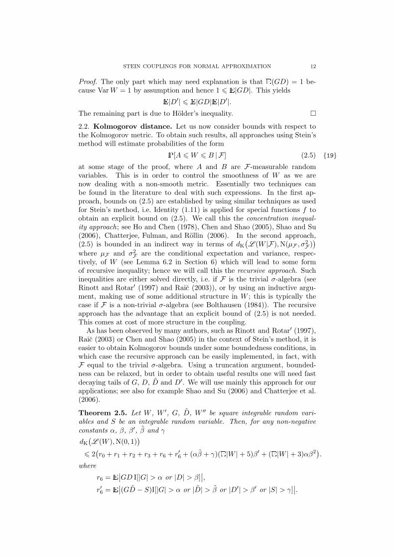
Proof. The only part which may need explanation is that E(GD) = 1 be-cause VarW = 1 by assumption and hence 1 6 E|GD|. This yieldsE|D′| 6 E|GD|E|D′|.The remaining part is due to Holder’s inequality.
2.2. Kolmogorov distance. Let us now consider bounds with respect tothe Kolmogorov metric. To obtain such results, all approaches using Stein’smethod will estimate probabilities of the formP[A 6W 6 B | F ] (2.5) 19at some stage of the proof, where A and B are F-measurable randomvariables. This is in order to control the smoothness of W as we arenow dealing with a non-smooth metric. Essentially two techniques canbe found in the literature to deal with such expressions. In the first ap-proach, bounds on (2.5) are established by using similar techniques as usedfor Stein’s method, i.e. Identity (1.11) is applied for special functions f toobtain an explicit bound on (2.5). We call this the concentration inequal-ity approach; see Ho and Chen (1978), Chen and Shao (2005), Shao and Su(2006), Chatterjee, Fulman, and Rollin (2006). In the second approach,(2.5) is bounded in an indirect way in terms of dK
(
L (W |F),N(µF , σ2F )
)
where µF and σ2F are the conditional expectation and variance, respec-tively, of W (see Lemma 6.2 in Section 6) which will lead to some formof recursive inequality; hence we will call this the recursive approach. Suchinequalities are either solved directly, i.e. if F is the trivial σ-algebra (seeRinott and Rotar′ (1997) and Raic (2003)), or by using an inductive argu-ment, making use of some additional structure in W ; this is typically thecase if F is a non-trivial σ-algebra (see Bolthausen (1984)). The recursiveapproach has the advantage that an explicit bound of (2.5) is not needed.This comes at cost of more structure in the coupling.
As has been observed by many authors, such as Rinott and Rotar′ (1997),Raic (2003) or Chen and Shao (2005) in the context of Stein’s method, it iseasier to obtain Kolmogorov bounds under some boundedness conditions, inwhich case the recursive approach can be easily implemented, in fact, withF equal to the trivial σ-algebra. Using a truncation argument, bounded-ness can be relaxed, but in order to obtain useful results one will need fastdecaying tails of G, D, D and D′. We will use mainly this approach for ourapplications; see also for example Shao and Su (2006) and Chatterjee et al.(2006).
Theorem 2.5. Let W , W ′, G, D, W ′′ be square integrable random vari-ables and S be an integrable random variable. Then, for any non-negativeconstants α, β, β′, β and γ
dK(
L (W ),N(0, 1))
6 2(
r0 + r1 + r2 + r3 + r6 + r′6 + (αβ + γ)(E|W |+ 5)β′ + (E|W |+ 3)αβ2)
.
where
r6 = E∣∣GD I[|G| > α or |D| > β]∣
∣,
r′6 = E∣∣(GD − S)I[|G| > α or |D| > β or |D′| > β′ or |S| > γ]∣
∣.

STEIN COUPLINGS FOR NORMAL APPROXIMATION 13
If a sequence of couplings (Wn,W′n, Gn,W
′′n , Dn, Sn)n>1 is under consider-
ation, the truncation points α, β, β′, β and γ will of course need to dependenton n. In a typical situation, say a sum of n bounded i.i.d. random variables,we will have α ≍ n1/2, β ≍ β′ ≍ β ≍ n−1/2 and γ ≍ 1.
Corollary 2.6. Let (W,W ′, G) be a Stein coupling with VarW = 1. If Gand D are bounded by positive constants α and β, respectively, then
dK(
L (W ),N(0, 1))
6 2√
VarEW (GD) + 8αβ2
Note that, even if G and D are bounded, we unfortunately cannot deducea direct, useful bound on VarEW (GD) from that fact. Instead, we needagain more structure in order to avoid VarEW (GD).
Corollary 2.7. Let (W,W ′, G) be a Stein coupling with VarW = 1 and
assume that there are D such that EW (GD) = EW (GD), S such thatEWS = 1 and W ′′ independent of (GD, S). If the absolute values of G,
D, D, D′ and S are bounded by α, β, β, β′ and γ, respectively, then
dK(
L (W ),N(0, 1))
6 8αβ2 + 12αββ′ + 12γβ′.
We need to emphasize the remarkable statement of Corollary 2.7: underthe conditions stated we immediately obtain a bound on the Kolmogorovdistance to the standard normal without any additional computations! Ex-amples can easily found such as bounded, locally dependent random vari-ables; see Section 3.2.
The approach we will use for the next theorem was developed by Chen and Shao(2004) for locally dependent random variables. Although a concentrationinequality approach was used by Chen and Shao (2004), the recursive ap-proach is easy to implement without loss of precision. Like in Theorem 2.5,the aim is to obtain a bound involving (2.5) with respect to the uncondi-tional W . This comes at the cost of truncated forth moments, especially inthe form of r8. Hence, the approach of avoiding truncated forth momentsby making use of W ′′ in r3 will not be useful because of the presence of r8.Therefore, we give below only a version for W ′′ = W , D = D and S = 1to avoid unnecessary overloading of the bound. To define some additionalerror terms, let
K(t) := G(I[0 6 t < D]− I[D 6 t < 0]), (2.6) 20KW (t) := EW K(t), K(t) := EK(t).
Theorem 2.8. Let W , W ′ and G be square integrable random variables onthe same probability space. Then
dK(
L (W ),N(0, 1))
6 2r0 + 2r3 + 2r4 + 2(E|W |+ 2.4)r5
+ 1.4r7 + 2((E(|W | + 1)2)1/2 + 1.1)r8
where r3 = E∣∣EW (GD)− 1∣
∣, where r4 and r5 are defined as in Theorem 2.1and where
r7 =
∫
|t|61VarKW (t)dt, r8 =
(∫
|t|61|t|VarKW (t)dt
)1/2
.

STEIN COUPLINGS FOR NORMAL APPROXIMATION 14
Let us discuss VarKW (t). Typically, W will consist of n parts, such asa sum of n random variables or a functional in n coordinates. In this case,the perturbation W ′ will typically be constructed by picking a small part ofW , say part I, where I is uniform on 1, . . . , n and then perturb this part.Thus, we typically will have G := nYI , D := DI for sequences Y1, . . . , Ynand D1, . . . ,Dn and then define W ′ := W +DI , where, with σ
2 = VarW ,E|Yi| = O(σ−1/2) and E|Di| = O(σ−1/2). Let now (W ∗,W ∗′, G∗) be anindependent copy of (W,W ′, G) and let I±t (x) = I[0 6 t < x]− I[x 6 t < 0].Then we can write
VarKW (t) 6n∑
i,j=1
Cov(YiI±t (Di), YjI
±t (Dj))
=
n∑
i,j=1
EYiYjI±t (Di)I±t (Dj)− YiY
∗j I
±t (Di)I
±t (D
∗j )
so that
r7 6
n∑
i,j=1
EYiYjI[DiDj > 0](|Di| ∧ |Dj | ∧ 1)
− YiY∗j I[DiD
∗j > 0](|Di| ∧ |D∗
j | ∧ 1)
and
r28 61
2
n∑
i,j=1
EYiYjI[DiDj > 0](|Di|2 ∧ |Dj |2 ∧ 1)
− YiY∗j I[DiD
∗j > 0](|Di|2 ∧ |D∗
j |2 ∧ 1)
,
respectively. In the case of local dependence, these quantities can now bebounded relatively easily; see Chen and Shao (2004).
If truncated fourth moments are to be avoided and no boundedness can beassumed, it seems that more structure is needed in the coupling. A typicalinstance is the use of higher-order neighbourhoods under local dependenceas in Chen and Shao (2004), or the recursive structure in the combinatorialCLT in Bolthausen (1984). The theorem below is the basis for such resultsand it contains expressions of the form (2.5) explicitly, so that further stepsare needed for a final bound.
Define for a random element X defined on the same probability spaceas W the quantity
ϑε(X) = supa∈RP[a 6W 6 a+ ε |X],
where we assume without further mentioning that the regular conditionalprobability exists.
Theorem 2.9. Let W , W ′, W ′′, D and G be random variables with finitethird moments and S be a random variable with E|S|3/2 < ∞. Then, forany ε > 0,
dK(
L (W ),N(0, 1))
6 r0 + r1 + r2 + r3 + r9 + 0.5r10 + ε−1r11(ε) + 0.5ε−1r12(ε) + 0.4ε(2.7) 21

STEIN COUPLINGS FOR NORMAL APPROXIMATION 15
where
r9 = E∣∣(S −GD)(|W |+ 1)(|D′| ∧ 1)∣
∣ r10 = E|G(|W | + 1)(D2 ∧ 1)|r11(ε) = E∣∣(S −GD)D′ϑε(G, D,D
′, S)∣
∣ r12(ε) = E∣∣GD2ϑε(G,D)∣
∣
We now look at a method to obtain a final bound from the above theoremusing induction. Although never mentioned in the literature around Stein’smethod, this type of argument can be traced back to Bergstrom (1944), whouses Lindeberg’s method and an inductive argument to prove a Kolmogorovbound in the CLT. The argument was used later by Bolthausen (1982) inthe context of martingale central limit theorems. The following Lemma 2.10provides the key element to the inductive approach in the context of Stein’smethod as introduced by Bolthausen (1984). It can be used to obtain afinal bound from an estimate of the form (2.7), provided that W = Wn
has some recursive structure and Sε can be expressed in terms of the close-ness of W1,W2, . . . ,Wn−1 to the standard normal distribution. Note thatin the following lemma, the numbers κk, k = 1, . . . , n denote the respectivebounds on the Kolmogorov distance between Wk and the standard nor-mal. Whereas Bolthausen (1984) uses a recursion involving κn−4, . . . , κn−1,Goldstein (2010) introduces a version involving all possible κ1, . . . , κn−1 toprove Berry-Esseen type bounds for degree counts in the Erdos-Renyi ran-dom graph using size biasing. Incidentally, already Bergstrom (1944) usesκ1, . . . , κn−1 for his inductive argument, although his argument is of a some-what different flavour. The following lemma is inspired by the work ofGoldstein (2010), but adapted to be used along with Theorem 2.9. Anindependent proof will be given in Section 6.
Lemma 2.10. Let κ1, . . . , κn, be a sequence of non-negative numbers suchthat κ1 6 1. Assume that there is a constant A > 0, a triangular arrayAk,1, . . . , Ak,k > 0, k = 2, 3, . . . , n, and a sequence σ2, . . . , σn > 0 such that,for all ε > 0 and all 2 6 k 6 n,
κk 6A
σk+ 0.4ε +
1
εσk
k−1∑
l=1
Ak,lκl. (2.8) 22
Then,
κn 61
σn
(
5(A ∨ 1) + 2αn + α′n
)(
2αn + α′n
)
5α′n
,
where
αn = sup26k6n
k−1∑
l=1
σkσlAk,l, α′
n =√
2αn(2αn + 5(A ∨ 1)).
Example 2.1. Let Wn = n−1/2∑n
i=1Xi where Xi are i.i.d. with EXi = 0and VarXi = 1 and E|Xi|3 = γ > 1. Let κn = dK
(
L (Wn),N(0, 1))
. Set
G = −n1/2XI and W ′ = W − n−1/2XI . Set also W ′′ = W ′, D = D andS = 1. Hence D = D′ = −n−1/2XI . We have
r0 = r1 = r2 = r3 = 0.
Furthermore,r9 6 6γ/
√n, r10 6 3γ/
√n

STEIN COUPLINGS FOR NORMAL APPROXIMATION 16
Note now (c.f. Lemma 6.2)
ϑε(Xn) = supaP[a 6Wn 6 a+ ε|Xn]
= supaP[√ n
n−1a 6Wn−1 +√
1n−1Xn 6
√
nn−1a+
√
nn−1ε+
∣
∣
∣Xn
]
6
√
n2π(n−1)ε+ 2κn−1 6 ε+ 2κn−1,
hence
r11(ε) 6 2γ(ε+ 2κn−1)/√n, r12(ε) 6 γ(ε+ 2κn−1)/
√n.
Putting these estimates into Theorem 2.9 we obtain
κk 68γ√k+ 0.4ε+
5γ
ε√kκk−1.
We can apply Lemma 2.10 with A = 8γ, Ak,k−1 = 5γ and Ak,l = 0 for
l < k − 1, and σk = k−1/2. We have αn = 5γ√2, thus, plugging this
into (2.8), κn 6 25γ/√n. As this example illustrates, the constants obtained
this way are typically not optimal, but nevertheless explicit.
3. Couplings
In this section we present some well-known and some new couplings andshow how they can be represented in our general framework. The basisis always the coupling (W,W ′, G) and throughout this section (with theexception of classic exchangeable pairs) we will only look at cases of actualStein couplings, that is, where r0 = 0. This implies in particular thatEW = 0 (which, nevertheless, has to be assumed explicitly in some casesto make the construction work in the first place). Unless otherwise stated,the variance σ2 of W is arbitrary, but finite and non-zero. Note that, if(W,W ′, G) is a Stein coupling, so is (W/σ,W ′/σ,G/σ), and hence we willusually omit the standardising constant σ−1 for ease of notation. To simplifyor optimize the bounds, we sometimes will extend the coupling by differentchoices of D, W ′′ and S. But, if not otherwise stated, we will make the basicassumption throughout this section that D = D, W ′′ =W and S = 1.
We mostly present the construction of the couplings only and not theparticular form of the final bounds for the normal approximation. The rea-son for this is that, once the coupling is constructed, one can directly applyour theorems or corollaries of the main section to obtain the correspond-ing bounds. Hence, stating them explicitly would be either just repeatingknown results from the literature or rephrasing the results from the mainsection.
We need to clarify again that a Stein coupling by itself does by no meansimply closeness to normality or imply any convergence. As can be seen fromthe case of quadratic forms (Section 3.2.3), Stein couplings as defined by(1.8) can also be used for χ2 approximation.
Let throughout this part [n] := 1, 2, . . . , n and [0] := ∅. Let also in gen-eral I and J be independent random variables, uniformly distributed on [n]and independent of all else, but we will usually mention this—and deviationsfrom it—explicitly whenever we make use of these random variables.

STEIN COUPLINGS FOR NORMAL APPROXIMATION 17
3.1. Exchangeable pairs and extensions. This approach was introducedby Stein in a paper by Diaconis (1977). A systematic exposition was givenby Stein (1986).
Construction 1A. Assume that (W,W ′) is an exchangeable pair. If, forsome constant λ > 0, we haveEW (W ′ −W ) = −λW, (3.1) 23then (W,W ′, 1
2λ (W′ −W )) is a Stein coupling.
Rinott and Rotar′ (1997) generalised (3.1) to allow for some non-linearityin (3.1); however, the resulting coupling will only be an approximate Steincoupling.
Construction 1B. Assume that (W,W ′) is an exchangeable pair whereEW = 0 and VarW = 1. Assume that, for some constant λ > 0, we haveEW (W ′ −W ) = −λW +R. (3.2) 24then, with G = 1
2λ(W′ −W )),
r0 6 λ−1E|R|, |E(GD) − 1| 6 λ−1|E(WR)| 6 λ−1√VarR.
(note that we use VarW = 1 only to obtain the last two inequalities).
The conditional expectation can of course always be written in the form of(3.2) for any λ. However, we will need λ−1
√VarR→ 0 to obtain convergent
bounds, and in this sense the choice of λ is, at least asymptotically, unique;see the discussion in the introduction of Reinert and Rollin (2009a).
Note that we call this approach ‘classic’ for this specific choice of G.There are many other ways to construct Stein couplings where (W,W ′) isexchangeable but G is not a multiple of W ′−W ; we will give such exampleslater on.
The classic exchangeable pairs approach is frequently used in the liter-ature; see for example Rinott and Rotar′ (1997), Fulman (2004a), Fulman(2004b), Rollin (2007b), Meckes (2008) and others. Generally, one con-structs a “natural” exchangeable pair (W ′,W ) and then hopes that (3.2)holds with R = 0 or R small enough to yield convergence. However, moreoften than not, this will not succeed, even for simple examples as the 2-runsexamples below illustrates. Based on work by Reinert and Rollin (2009a),we will present in Section 3.1.1 Stein couplings making use of a multivariateextensions of (3.1) which will lead to appropriate modifications of G suchthat (1.8) holds. In Sections 3.2.4 and 3.4 we will also present two very gen-eral couplings that are based on exchangeable pairs, but where G is chosenrather differently.
A few more detailed remarks about this approach are appropriate here.For this specific choice of G = (W ′ − W )/2λ, Rollin (2008a) proves thatexchangeability is actually not necessary to prove a result such as The-orem 2.5, as long as we have equal marginals L (W ′) = L (W ). Rollin(2008a) uses a different way of deducing a Stein identity of the form (1.11).With F (w) =
∫ w0 f(x)dx one obtains from Taylor’s expansion that
F (W ′)− F (W ) = Df(W ) +D
∫ D
0(1− s/D)f ′(W + s)ds,

STEIN COUPLINGS FOR NORMAL APPROXIMATION 18
so that, again with G = D/2λ, and assuming L (W ′) = L (W ),EGf(W ) = EG∫ D
0(1− s/D)f ′(W +D)ds
, (3.3) 25
which serves as a replacement for (1.11). In contrast, Stein (1986) uses theantisymmetric function approach. If (W,W ′) is exchangeable then E(W ′−W )(f(W ′) + f(W ))
= 0, and it is not difficult to show thatEGf(W ) =1
2EG∫ D
0f ′(W +D)ds
. (3.4) 26
Note that this is almost (3.3) except that the factor (1 − s/D) is replacedby 1/2. Note again that (3.4) is only true under exchangeability whereas(3.3) holds for equal marginals. Surprisingly, better constants can be ob-tained if (3.3) is used instead of (3.4), although exchangeability is a strongerassumption. Incidentally, in Section 4.4, a coupling is used which is not anexchangeable pair but has equal marginals, however, in the context of adifferent construction than Construction 1A.
3.1.1. Multivariate exchangeable pairs. In Reinert and Rollin (2009a), theclassic exchangeable pairs approach was generalised to d-dimensional vectorsW = (W1, . . . ,Wd) and W
′ = (W ′1, . . . ,W
′d) which satisfyEW (W ′ −W ) = −ΛW (3.5) 27b
for some invertible (d × d)-matrix Λ. They are able to obtain multivari-ate normal approximation results in cases where the exchangeable pair ofunivariate random variables (W1,W
′1) does not satisfy (3.1), but, using aux-
iliary random variates, an embedding of that pair into a higher dimensionalspace satisfies (3.5). However, the transition to higher dimensions comes atthe cost of having to impose stronger conditions on the set of test functions.Hence, besides the multivariate approximation, it is therefore still of inter-est to examine W1 directly. It turns out that, once the higher dimensionalembedding satisfying (3.5) is found, it is easy to construct a Stein couplingfrom that.
Construction 1C. Let (W,W ′) be an exchangeable pair of d-dimensionalrandom vectors satisfying (3.6) for some invertible Λ. Let ei be the i-th unitvector. Then
(
Wi,W′i ,
12e
tiΛ
−1(W ′ −W ))
is a Stein coupling.
Indeed,
−EGf(Wi)
= −12EetiΛ−1EW (W ′ −W )f(Wi)
= 12EetiΛ−1ΛWf(Wi)
= 12EWif(Wi)
.
and, using exchangeability, the corresponding result for EGf(W ′i )
can beobtained in the same way. Hence, every multidimensional exchangeable pair(W,W ′) satisfying (3.5) gives rise to a univariate Stein coupling for eachindividual coordinate.
Let us consider the case of 2-runs on a circle. To this end, let ξ1, . . . , ξnbe a sequence of independent Be(p) distributed random variables. Let V =

STEIN COUPLINGS FOR NORMAL APPROXIMATION 19
∑ni=1(ξiξi+1−p2) be the centered number of 2-runs, where we put ξn+1 = ξ1
(hence ‘circle’). Consider now the following coupling. With ξ′1, . . . , ξ′n being
independent copies of ξ1, . . . , ξn, let V′ = V − ξI−1ξI − ξIξI+1 + ξI−1ξ
′I +
ξ′IξI+1, where I is uniformly distributed on [n] and independent of all else.It is easy to see that (V, V ′) is an exchangeable pair and thatEV (V ′ − V ) = − 2
nV +
2p
n
n∑
i=1
(ξi − p). (3.6) 27
Even in this very simple example, the linearity condition (3.2) cannot beobtained with the above natural coupling. Based on the same exchangeablepair, Reinert and Rollin (2009a) use the embedding method to circumventthis problem. To this end we introduce the auxiliary statistic U =
∑ni=1(ξi−
p) and define U ′ = U − ξI + ξ′I . Condition (3.5) is now satisfied for W =(U, V ), W ′ = (U ′, V ′) and
Λ =1
n
[
1 0
−2p 2
]
.
The inverse of Λ is
Λ−1 = n
[
1 0
p 1/2
]
,
hence Construction 1C yields
G =n
2
(
p(U ′ − U) + 12(V
′ − V ))
=n
2
(
pξ′I − pξI +12ξI−1ξ
′I +
12ξ
′IξI+1 − 1
2ξI−1ξI − 12ξIξI+1
)
(3.7) 27d
so that (V, V ′, G) is a Stein coupling. Exploiting some specific properties inthis example, we may also choose
G =n
2
(
pξ′I − pξI + ξ′IξI+1 − ξIξI+1
)
(3.8) 27c
to obtain a somewhat simpler Stein coupling, but the similarity between(3.7) and (3.8) is apparent. See Reinert and Rollin (2009a), Reinert and Rollin(2009b) and Ghosh (2010) for further examples of multivariate exchangeablepair couplings.
3.1.2. Finding W for a given coupling and a given G. In some cases it maynot be clear from the beginning how to choose the main random variableof interest W . Consider the Curie-Weiss model of ferromagnetic interac-tion. With β > 0 being the inverse temperature and h ∈ R the exter-nal field on the state space −1, 1n, we define the probabilities for eachσ = (σ1, . . . , σn) ∈ −1, 1n by the Gibbs measureP[σ] = Z−1 exp
β
n
∑
i<j
σiσj + h∑
i
σi
(3.9) 28
where Z = Z(β, h, n) is the partition function to make the probabilities sumup to 1. A quantity of interest is the magnetization m(σ) = n−1
∑
i σi ∈[−1, 1] of the system. However, in the low-temperature regime the systemwill exhibit spontaneous magnetization so that we may not be interested inm(σ) itself if σ is drawn at random according to (3.9) but inm(σ) relative to

STEIN COUPLINGS FOR NORMAL APPROXIMATION 20
its corresponding magnetization. To find a suitable correction term (whichshall serve here as an illustrative example only), Chatterjee (2007) proposesthe following construction.
Construction 1D. Let (σ, σ′) be an exchangeable pair on some measurespace and let ϕ(σ, σ′) be an anti-symmetric function. Let G = −ϕ(σ, σ′)/2,W =W (σ) = Eσϕ(σ, σ′) and W ′ =W (σ′) = Eσ′
ϕ(σ′, σ). Then this definesa Stein coupling.
Indeed,
−EGf(W )
= 12Eϕ(σ, σ′)f(W )
= 12EWf(W )
and EGf(W ′)
= −12Eϕ(σ, σ′)f(W (σ′))
= −12Eϕ(σ′, σ)f(W (σ))
= 12Eϕ(σ, σ′)f(W )
= 12EWf(W )
,
which proves (1.8).Let us apply this to the Curie-Weiss model. First, given σ is drawn from
(3.9), we define σ′ by choosing a site I uniformly at random and then we re-sample this site according to the conditional distribution L (σI |σj, j 6= I),giving a new σ′I , but leaving all the other sites untouched. Now we setϕ(σ, σ′) = n(m(σ)−m(σ′)) = σI − σ′I . It is not difficult to show thatEσϕ(σ, σ′) = m(σ)− 1
n
∑
i
tanh(βmi(σ) + βh),
where mi(σ) =1n
∑
j 6=i σj . Hence, we let G = −(σI − σ′I)/2,
W =W (σ) = m(σ)− 1
n
∑
i
tanh(βmi(σ) + βh),
and W ′ :=W (σ′). As∣
∣
∣tanh(βm(σ) + βh) − 1
n
∑
i
tanh(βmi(σ) + βh)∣
∣
∣6β
n,
we may alternatively choose W = m(σ)− tanh(βm(σ) + βh), in which case(1.8) is not satisfied anymore, but we still have r0 6 β/n. The key hereis to find ϕ(σ, σ′) such that Eσϕ(σ, σ′) yields ‘something interesting’. InChatterjee (2007) this construction is used to prove concentration of measureresults for such W .
3.1.3. Finding an antisymmetric G through a Poisson equation. Assumenow that (X,X ′) is an exchangeable pair on some space X and W = ϕ(X)and W ′ = ϕ(X ′) for some functional ϕ : X → R with Eϕ(X) = 0.Chatterjee (2005, Section 4.1) proposes a general approach to find G ofa special form. Let G(X ′,X) = 1
2(ψ(X′) − ψ(X)) for some unknown func-
tional ψ : X → R (in fact, any anti-symmetric function can be written inthis form; see Stein (1986)). Using exchangeability, it is not difficult to seethat (1.8) is satisfied if
ψ(x) − Pψ(x) = ϕ(x)

STEIN COUPLINGS FOR NORMAL APPROXIMATION 21
for every x ∈ X , which we recognize as a Poisson equation with kernelPψ(x) := EX=xψ(X ′) for given ϕ and unknown ψ. A general (formal)solution is ψ(x) =
∑∞k=0 P
kϕ(x). We have the following.
Construction 1E. Let (X,X ′) be an exchangeable pair on a measure spaceX and let ϕ : X → R be a measurable function such that Eϕ(X) = 0; defineP as above. If there is a constant C > 0 such that
∞∑
k=0
|P kϕ(x)− P kϕ(y)| 6 C (3.10) 29
for every x, y ∈ X , then
(W,W ′, G) =(
ϕ(X), ϕ(X ′),1
2
∞∑
k=0
(
P kϕ(X) − P kϕ(X ′))
)
is a Stein coupling.
Note that boundedness |G| 6 C/2 is built in through (3.10) so that thisconstruction is a natural candidate for Theorem 2.5. We can give a moreconstructive version of this coupling.
Construction 1F. Assume that (X,X ′), ϕ and P are as in Construc-tion 1E. Assume that we have two Markov chains
(
Xn
)
n>0and
(
X ′n
)
n>0
with the transition dynamics given by P , and also X0 = X and X ′0 = X ′.
Assume further that, for all n,
L(
Xn
∣
∣X,X ′)
= L(
Xn
∣
∣X)
, L(
X ′n
∣
∣X,X ′)
= L(
X ′n
∣
∣X ′)
. (3.11)
Let now T = inf
n > 0∣
∣ Xn = X ′n
be the coupling time of the two chainsand assume that T <∞ almost surely. If, given T , I is uniformly distributedon 0, 1, 2, . . . , T − 1, then
(W,W ′, G) =(
ϕ(X), ϕ(X ′), 12T(
ϕ(XI)− ϕ(X ′I)))
(3.12) 30
is a Stein coupling.
Indeed, from Eϕ(Xk)f(W )
= EP k(X)f(W )
and Eϕ(X ′k)f(W )
= Ef(W )EX,X′ϕ(X ′
k)
= Ef(W )P kϕ(X ′)
,
we easily obtainET (ϕ(XI)− ϕ(X ′I))
f(W )
= E T−1∑
k=0
(
ϕ(Xk)− ϕ(X ′k))
f(W )
=
∞∑
k=0
E(ϕ(Xk)− ϕ(X ′k))
f(W )
=
∞∑
k=0
E(P kϕ(X) − P kϕ(X ′))
f(W )
,

STEIN COUPLINGS FOR NORMAL APPROXIMATION 22
and, similarly,ET (ϕ(XI)− ϕ(X ′I))
f(W ′)
=
∞∑
k=0
E(P kϕ(X) − P kϕ(X ′))
f(W ′)
= −∞∑
k=0
E(P kϕ(X) − P kϕ(X ′))
f(W )
,
where the second step uses exchangeability. Hence, it follows from Construc-tion 1E that (3.12) is a Stein coupling; see Chatterjee (2005, Section 4.1) formore details, and see also Makowski and Shwartz (1994) on general theoryabout Poisson equations.
3.2. Local dependence and related couplings. This is one of the earli-est versions of Stein’s method. Let in what follows I be uniformly distributedon [n], independent of all else.
Construction 2A. Let W =∑n
i=1Xi with EXi = 0. For each i, let W ′i be
such that E(Xi |W ′i
)
= 0. (3.13) 31Then, (W,W ′, G) = (W,W ′
I ,−nXI) is a Stein coupling.
To see this we have on one hand
−EGf(W )
=
n∑
i=1
EXif(W )
= EWf(W )
, (3.14) 32
and on the other handEGf(W ′)
= −n∑
i=1
EXif(W′i )
= 0,
due to (3.13); hence (1.8) is satisfied.The choice G = −nXI was first considered by Stein (1972) form-dependent
sequences, however this G has broader applications. We now discuss somemore detailed constructions of W ′
i below.
3.2.1. Local dependence. Local dependence was extensively studied in Chen and Shao(2004) under various dependence settings, but of course this approach goesback to Stein (1972) and Chen (1975); a version for discrete random vari-ables is given by Rollin (2008b). We can use the simplest form as a startingpoint
Construction 2B. Assume that W and G are as in Construction 2A. As-sume in addition that, for each i ∈ [n], there is Ai ⊂ [n] such that Xi
and (Xj)j∈Aciare independent. Then, with W ′
i = W −∑
j∈AiXj, (3.13) is
satisfied.
This first-order dependence is usually referred to as (LD1) and is enoughto obtain a Stein coupling. However, it is possible to extend this coupling.
Construction 2C. Assume that W and G and Wi are as in Construc-tions 2A and 2B and that VarW = 1. Assume in addition that there isBi ⊂ [n] such that Ai ⊂ Bi and (Xj)j∈Ai
and (Xj)j∈Bciare independent.
Define W ′′i = W − ∑
j∈BiXj ; then W ′′ := W ′′
I is independent of GD andhence r3 = 0.
STEIN COUPLINGS FOR NORMAL APPROXIMATION 23
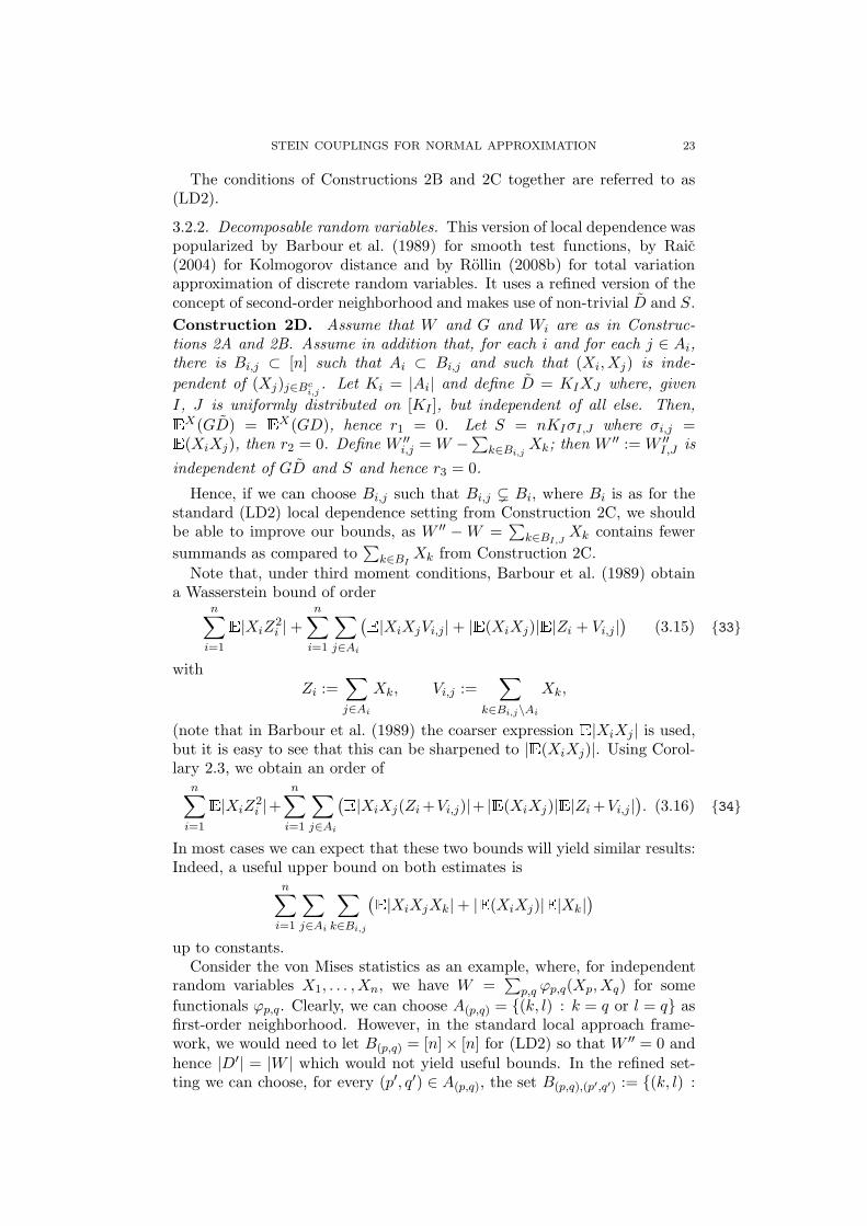
The conditions of Constructions 2B and 2C together are referred to as(LD2).
3.2.2. Decomposable random variables. This version of local dependence waspopularized by Barbour et al. (1989) for smooth test functions, by Raic(2004) for Kolmogorov distance and by Rollin (2008b) for total variationapproximation of discrete random variables. It uses a refined version of theconcept of second-order neighborhood and makes use of non-trivial D and S.
Construction 2D. Assume that W and G and Wi are as in Construc-tions 2A and 2B. Assume in addition that, for each i and for each j ∈ Ai,there is Bi,j ⊂ [n] such that Ai ⊂ Bi,j and such that (Xi,Xj) is inde-
pendent of (Xj)j∈Bci,j. Let Ki = |Ai| and define D = KIXJ where, given
I, J is uniformly distributed on [KI ], but independent of all else. Then,EX(GD) = EX(GD), hence r1 = 0. Let S = nKIσI,J where σi,j =E(XiXj), then r2 = 0. Define W ′′i,j =W −∑
k∈Bi,jXk; then W
′′ :=W ′′I,J is
independent of GD and S and hence r3 = 0.
Hence, if we can choose Bi,j such that Bi,j ( Bi, where Bi is as for thestandard (LD2) local dependence setting from Construction 2C, we shouldbe able to improve our bounds, as W ′′ −W =
∑
k∈BI,JXk contains fewer
summands as compared to∑
k∈BIXk from Construction 2C.
Note that, under third moment conditions, Barbour et al. (1989) obtaina Wasserstein bound of order
n∑
i=1
E|XiZ2i |+
n∑
i=1
∑
j∈Ai
(E|XiXjVi,j|+ |E(XiXj)|E|Zi + Vi,j|)
(3.15) 33
withZi :=
∑
j∈Ai
Xk, Vi,j :=∑
k∈Bi,j\Ai
Xk,
(note that in Barbour et al. (1989) the coarser expression E|XiXj | is used,but it is easy to see that this can be sharpened to |E(XiXj)|. Using Corol-lary 2.3, we obtain an order of
n∑
i=1
E|XiZ2i |+
n∑
i=1
∑
j∈Ai
(E|XiXj(Zi+Vi,j)|+ |E(XiXj)|E|Zi+Vi,j|)
. (3.16) 34
In most cases we can expect that these two bounds will yield similar results:Indeed, a useful upper bound on both estimates is
n∑
i=1
∑
j∈Ai
∑
k∈Bi,j
(E|XiXjXk|+ |E(XiXj)|E|Xk|)
up to constants.Consider the von Mises statistics as an example, where, for independent
random variables X1, . . . ,Xn, we have W =∑
p,q ϕp,q(Xp,Xq) for some
functionals ϕp,q. Clearly, we can choose A(p,q) = (k, l) : k = q or l = q asfirst-order neighborhood. However, in the standard local approach frame-work, we would need to let B(p,q) = [n]× [n] for (LD2) so that W ′′ = 0 andhence |D′| = |W | which would not yield useful bounds. In the refined set-ting we can choose, for every (p′, q′) ∈ A(p,q), the set B(p,q),(p′,q′) := (k, l) :

STEIN COUPLINGS FOR NORMAL APPROXIMATION 24
k ∈ p, p′ or l ∈ q, q′, so that now |B(p,q),(p′,q′)| is only of order n. Ofcourse, it will depend on the concrete choice of functionals ϕp,q whethernormal approximation is appropriate at all; see Barbour et al. (1989) forapplications to random graph related statistics.
3.2.3. Special case: quadratic forms. Let ξ1, . . . , ξn be independent, centeredrandom variables with unit variance. Let A = (aij) be a real symmetric(n×n)-matrix. LetW =
(∑
i,j aijξiξj−∑
i aii)
. It would be straightforwardto use the above method of decomposable random variables in this situation.However, due to the multiplicative structure (or, in U -statistics language,because the kernel ϕi,j(x, y) = aijxy is degenerate for centered randomvariables) there is an interesting alternative.
Construction 2E. Let W be as above. Let also Yi :=∑
j aijξj, G =
−n(ξIYI − aII) and W ′ = W − (2ξIYI − aIIξ2I ). Then this defines a Stein
coupling.
It is not difficult to see that (1.8) holds. Again, it depends on the matrixA whether we can expect normal like behaviour ofW or not: essentially thiscoupling was used by Luk (1994) in the context of χ2-approximation for thecase where all the entries of A are 1, corresponding to the square of a sumof random variables.
3.2.4. Local exchangeable randomization. This coupling was proposed in Reinert(1998). Its use was limited by the fact that, if the classic exchangeable pairsapproach (as discussed in Subsection 3.1) is used along with this coupling,the linearity condition (3.2) will in general not be satisfied with R smallenough, but with the choice G = −nXI , we can now handle this coupling.However, some care is needed.
Construction 2F. Let W and G be as in Construction 2A. Let (X ′i,j)i,j∈[n]
be a collection of random variables, such that, with W ′i =
∑nj=1X
′i,j, we
have that
(i) for each i, X ′i,i is independent of W , (3.17) 37
(ii) for each i,(
(Xk)k, (X′i,k)k
)
is exchangeable. (3.18) 38
Then (3.13) is satisfied.
It is often not too difficult to construct (X ′i,j)j for a given i such that
L (W ′i ) = L (W ) and such thatX ′
i,i is independent ofW and henceEWX ′i,i =
0. However, it is important to note that this does not suffice as we ultimatelyneed EW ′
iXi = 0, which is, however, guaranteed under the additional Con-dition (3.18).
In Reinert (1998), it was incorrectly deduced from (3.17) and the property
L (X ′i,j , j 6= i |X ′
i,i = x) = L (Xj , j 6= i |Xi = x) (3.19) 39
that (W,W ′i ) is exchangeable. It is not difficult to find examples for which
(W,W ′i ) is not exchangeable, but (3.17) and (3.19) are still true; see Re-
mark 4.2.

STEIN COUPLINGS FOR NORMAL APPROXIMATION 25
3.3. Size-biasing. This approach was introduced in Baldi, Rinott, and Stein(1989) and further explored in Goldstein and Rinott (1996), Dembo and Rinott(1996), Goldstein and Penrose (to appear) and others.
Construction 3A. Let V be a non-negative random variable with EV =µ > 0. Let V s have the size-biased distribution of V , that is, for allbounded f , EV f(V )
= µEf(V s). (3.20) 40Then
(W,W ′, G) =(
V − µ, V s − µ, µ)
is a Stein coupling.
Using (3.20), we obtainEGf(W ′)−Gf(W )
= Eµf(V s − µ)− µf(V − µ)
= EV f(V − µ)− µf(V − µ)
= EWf(W )
,
so that (1.8) is satisfied, indeed.One of the advantages of this approach is apparent if bounds for the Kol-
mogorov metric are to be obtained. In the light of Theorem 2.1, we see thatG/σ is already bounded by α = µ/σ, so that we only need to concentrate onfinding a bounded coupling (W,W ′); see Goldstein and Penrose (to appear)for such a coupling in the context of coverage problems.
3.4. Interpolation to independence. For this coupling the key idea is toconstruct a sequence of random variables that ‘interpolates’ between W andan independent copy of W by means of small perturbations. A special caseof this coupling was introduced by Chatterjee (2008). The construction hasapparent similarities to Lindeberg’s telescoping sum in his prove of the CLTfor sums of independent random variables. Let in the following constructionI be uniformly distributed on [n] and independent of all else.
Construction 4A. Assume EW = 0. Assume that for each i ∈ [n] we havea W ′
i which is close to W . Assume that there is a sequence of random vari-ables V0, V1, . . . , Vn such that EWV0 = W and such that Vn is independentof V0 and assume that, for every i ∈ [n],
L[
(W,Vi−1), (W′i , Vi)
]
= L[
(W ′i , Vi), (W,Vi−1)
]
(3.21) 42for every i ∈ [n]. Then
(W,W ′, G) =(
W,W ′I ,
n2 (VI − VI−1)
)
(3.22) 43is a Stein coupling.
Note that (3.21) implies in particular that (W,W ′i ) is an exchangeable
pair for each i and also that L (Vi) = L (V0) for all i by induction. We haveEGf(W )
= 12E n
∑
i=1
(Vi − Vi−1)f(W )
= 12E(Vn − V0)f(W )
= −12EWf(W )
,

STEIN COUPLINGS FOR NORMAL APPROXIMATION 26
due to the independence assumption, and, due to (3.21),EGf(W ′)
=1
2
n∑
i=1
E(Vi − Vi−1)f(W′i )
=1
2
n∑
i=1
E(Vi−1 − Vi)f(W )
= −1
2
n∑
i=1
E(Vi − Vi−1)f(W )
= −EGf(W )
= 12EWf(W )
.
Hence, (3.22) is a Stein coupling, indeed.
3.4.1. Functionals of independent random variables. A specific version ofthis coupling was used by Chatterjee (2008) for functionals of independentrandom variables. We give a simpler version first and discuss then the(implicitly used) coupling of Chatterjee (2008).
Construction 4B. Let X = (X1, . . . ,Xn) be a collection of independentrandom variables and let W = F (X) be any functional of X such thatEF (X) = 0. Let X ′ = (X ′
1, . . . ,X′n) be an independent copy of X and
define for all subsets A ⊂ [n] the vectors XA = (XA1 , . . . ,X
An ) by
XAi =
X ′i if i ∈ A,
Xi if i /∈ A,
that is, XA is simply X but with all Xi replaced by X ′i for which i ∈ A;
define also W ′A = F (XA). Let W ′
i := W ′i for each i ∈ [n] and Vi := W ′
[i]
for each i ∈ [n]∪0. Then the conditions of Construction 4A are satisfied.
Clearly, Vn is independent of V0 and it is not difficult to see that (3.21)holds. The interpolating sequence is therefore constructed simply by re-placing the Xi by X
′i in increasing order. For this coupling to be useful we
would typically need that F is not too sensitive to changes in the individualcoordinates.
The implicit coupling used by Chatterjee (2008) is different in the sensethat, instead of using a fixed order in which the Xi are replaced, a randomorder is used.
Construction 4C. Assume that W , F , X and X ′ are as in 4B. Let Π be auniformly drawn random permutation of length n, independent of everythingelse. For any permutation π we denote by π(A) simply the image of Awith respect to π. Define now W ′
i := W ′Π(i) and Vi := W ′
Π([i]). Then the
conditions of Construction 4A are satisfied.
Exchangeability (3.21) follows from Construction 4B by conditioning on Π.Let us now prove that Construction 4C indeed leads to the representationused by Chatterjee (2008). Clearly, G = 1
2n(W′Π([I]) −W ′
Π([I−1])), thusEX,X′(GD) =
1
2n!
n∑
i=1
∑
π
(W ′π([i]) −W ′
π([i−1]))(W −W ′π(i)).

STEIN COUPLINGS FOR NORMAL APPROXIMATION 27
We re-write the sum over all permutation as a sum over all possible subsetsinduced by π([i−1]), that is, all possible subsets A ⊂ [n] with |A| = i−1, andover all possible values of π(i) which range over [n]\A. Taking into accountmultiplicities from all possible permutations within the sets π([i − 1]) andπ([n] \ [i]) we obtainEX,X′
(GD)
=1
2n!
n∑
i=1
∑
A⊂[n],|A|=i−1
∑
j /∈A
|A|!(n − |A| − 1)!(W ′A∪j −W ′
A)(W −W ′j)
=1
2
∑
A([n]
∑
j /∈A
1(
n|A|
)
(n − |A|) (W′A∪j −W ′
A)(W −W ′j),
which is exactly the expression used by Chatterjee (2008, Eq. (1)).
3.5. Local symmetry. An instance of this coupling was used by Chen(1998) for sums of independent random variables.
Construction 5A. Assume that W , W ′, Gα and Gβ are random variablessuch that EGαf(W
′) = EGβf(W′), (3.23) 45EGαf(W ) = EWf(W ), (3.24) 46EGβf(W ) = 0, (3.25) 47
for all f for which the expectations exist. Then, (W,W ′, Gβ−Gα) is a Steincoupling.
Indeed, using (3.23) for the first equality and then (3.24) and (3.25),E(Gβ −Gα)(f(W′)− f(W )) = E(Gα −Gβ)f(W ) = EWf(W ).
Note that we refer to Condition (3.23) as local symmetry due to the followingexample.
Let X = (X1, . . . ,Xn) be a sequence of centered independent randomvariables and let X ′ be an independent copy of X. Let W =
∑
iXi andassume that VarW = 1. Define Gα = XI and W ′ =W +X ′
I (we ‘duplicate’a small part of W ). Define also Gβ = X ′
I . Then it is not difficult to verifyConditions (3.23) and (3.24). Identity (3.23) is due to the symmetry of Gα
and Gβ relative to W ′, which is the crucial aspect of the construction.
3.6. Abstract approaches. One might wonder if, for a given arbitrarycoupling (W,W ′), one can always find G to make (W,W ′, G) a Stein cou-pling.
Construction 6A. Let (W,W ′) be a pair of integrable random variables.Let F and F ′ be two σ-algebras with σ(W ) ⊂ F and σ(W ′) ⊂ F ′. Let V bea random variable such that EWV =W. (3.26) 47bDefine (formally) the random variable
G = −V +E(V |F ′)−E(E(V |F ′)|F) +E(E(E(V |F ′)|F)|F ′)− . . . .

STEIN COUPLINGS FOR NORMAL APPROXIMATION 28
Construction W ′ D= W (W ′,W )
exchangeableW ′′ D
= W
Hoeffding (Var. 1) 1A (p. 17) yes yes –
Hoeffding (Var. 2) 2F (p. 24) yes yes –
Hoeffding (Var. 3) 5A (p. 27) no no yes
Occupancy 2F (p. 24) yes yes yes
Neighbourhood 2A (p. 22) no no no
Random graphs 2A (p. 22) yes no yes
Table 1. Overview over the couplings used in the differentapplications along with some interesting properties of theinvolved random variables.
If the above sequence converges absolutely almost surely, then (W,W ′, G) isa Stein coupling.
To see this, first condition G on F ′ which yields E(G|F ′) = 0. On theother hand, E(G|F) = −E(V |F) hence EWG = −W and (1.8) follows.Note that (3.26) is not to be confused with the usual linearity condition(3.1)—we can always take V =W to satisfy (3.26).
Consider the example W =∑n
i=1Xi, a sum of independent, centeredrandom variables. With I independent and uniformly distributed on [n], letW ′ =W −XI . Take V =W and note thatE(W |W ′) = E(W ′ +XI |W ′) =W ′, E(W ′|W ) = (1− 1
n)W.
Hence,
−G =W −W ′ + (1− 1n)W − (1− 1
n)W′ + (1− 1
n)2W − (1− 1
n)2W ′ + . . .
= XI + (1− 1n)XI + (1− 1
n)2XI + · · · = nXI .
Alternatively, chosing V = nXI yields the same result directly, as EW ′V = 0
and hence G = −V = −nXI .
4. Applications
In this section we give some applications of the main theorems and corol-laries using different couplings from Section 3. Table 1 gives an overviewover the different couplings we use in this section along with some importantcharacteristics of the involved random variables.
4.1. Hoeffding’s combinatorial statistic. Let ai,j, 1 6 i, j 6 n, be real
numbers such that∑n
k=1 ai,k =∑n
k=1 ak,j = 0 and 1n−1
∑
i,j a2i,j = 1. Let π
be a uniformly chosen random permutation of size n and W =∑n
i=1 ai,π(i).Then it is routine to see that EW = 0 and VarW = 1. Note that, for a Steincoupling (W,W ′, G), unit variance of W implies E(GD) = 1. Let in whatfollows I1 and I2 be independent and uniformly chosen random numbersfrom [n].

STEIN COUPLINGS FOR NORMAL APPROXIMATION 29
Variant 1 (c.f. Construction 1A). Define π′ = π (I1 I2) and W ′ =∑n
i=1 ai,π′(i). Then (W,W ′) is a classical exchangeable pair, i.e. (3.1) holdswith λ = 2/n, or, equivalently, G = n
4 (W′ −W ) = n
4 (aI1,π(I2) + aI2,π(I1) −aI1,π(I1) − aI2,π(I2)) makes (W,W ′, G) a Stein coupling.
Variant 2 (c.f. Construction 2F). Define W ′ as in Variant 1. WithG = −naI1,π(I1), (W,W ′, G) is also a Stein coupling. This coupling is the(implicit) basis for the construction in Ho and Chen (1978) and Bolthausen(1984).
In both of the previous variants, our W ′ is defined with respect to aperturbation π′ of π. Thus,W ′ can be seen as an instance of the replacementperturbation from the introduction. This comes at the cost of D havingfour terms. One may wonder whether a deletion construction is possible,where W ′ is defined by just ‘removing a random small part’ of W (seeSection 3.2.1). This is possible, indeed, so that we do not need to go throughconstructing π′. Despite the fact that the following construction is verysimple, it has gone unnoticed in the literature so far.
Variant 3 (c.f. Construction 5A). Define
W ′ =W −
(aI1,π(I1) + aI2,π(I2)) if I1 6= I2,
aI1,π(I1) if I1 = I2.
Let G = n(aI1,π(I2) − aI1,π(I1)); then (W,W ′, G) is a Stein coupling. To
see this, note first that σ(W ′) ⊂ F := σ(
I1, I2, (π(i); i 6= I1, I2))
. Now, ifI1 6= I2, the conditional distributions L (π(I1)|F) and L (π(I2)|F) are equaland assign probability 1/2 to each of the points in the set π(I1), π(I2)so that EGf(W ′) = 0. The same arguments from Variant 1 lead toEGf(W ) = −EWf(W ).
To see the connection with Construction 5A, let Gα = naI1,π(I1) andGβ = naI1,π(I2); then (3.23)–(3.25) are satisfied.
Let us quickly illustrate how to obtain a bound in terms of
‖a‖ := sup16i,j6n
|ai,j |.
With the Stein coupling from Variant 3 we have
|G| 6 2n‖a‖ =: α, |D| 6 2‖a‖ =: β.
We will make use of an auxiliary variable W ′′, which can be constructed sothat it is independent of (I1, I2, π(I1), π(I2)) and such that
|D′| 6 8‖a‖ =: β′. (4.1) 49Hence, applying Theorem 2.5 with the above random variables and constantsand in addition D = D and β = β we easily obtain the following result.
Theorem 4.1. With W and ‖a‖ as above,
dK(
L (W ),N(0, 1))
6 448n‖a‖3 + 96‖a‖.Proof. We only need the existence of W ′′ as claimed above; we use the con-struction of Bolthausen (1984). It turns out that it is more convenient toconstruct W from W ′′. Let τ be a uniformly chosen random permutation of

STEIN COUPLINGS FOR NORMAL APPROXIMATION 30
[n] and let W ′′ =∑
i ai,τ(i). Let (I1, I2, J1, J2) be random variables indepen-
dent of τ such that (I1, I2, J1) is uniform on [n]3, such that J2 is uniform on[n]\J1 if I1 6= I2 and such that J1 = J2 if I1 = I2. One can now constructa permutation π which again has uniform distribution, and such that
π(I1) = J1, π(I2) = J2,
and such that τ and π differ in at most four positions. Now Eτ (G3(W′3 −
W )) = E(G3(W′3 − W )) (and hence r3 = 0) follows from the indepen-
dence assumption between τ and (I1, I2, J1, J2). Note that the calculationsfrom Variant 3 above still hold, as, given π, (I1, I2) is uniformly distributedon [n]2, hence independent of π as required.
Remark 4.1. Note that Goldstein (2005), using zero-biasing, obtains
dK(
L (W ),N(0, 1))
6 1016‖a‖ + 768‖a‖2.4.2. Functionals in the classic occupancy scheme. Let m balls be dis-tributed independently of each other into n boxes such that the probability oflanding in box i is pi, where
∑ni=1 pi = 1. The literature on this topic is rich;
see for example Johnson and Kotz (1977), Kolchin, Sevast′yanov, and Chistyakov(1978) or Barbour, Holst, and Janson (1992), but also more recent resultssuch as Hwang and Janson (2008) and Barbour (2009) on local limits theo-rems for infinite number of urns. If ξi denotes the number of balls in urn iafter distributing the balls, some interesting statistics can be written in theform
U =
n∑
i=1
h(ξi)
for functions h : Z+ → R. Examples are
h(x) = I[x = k] “# urns with exactly k balls”,
h(x) = I[x > m0] “# urns exceeding a limit m0”,
h(x) = I[x > m0](x−m0) “# excess balls when urn limit is m0”;
see for example Boutsikas and Koutras (2002).Let us consider here the more general case
U =
n∑
i=1
hi(ξi) (4.2) 52
for functions hi : Z+ → R, i = 1, . . . , n. Due to the subsequent centering,we may assume without loss of generality that hi(0) = 0 for all i.
Theorem 4.2. Assume the situation as described above. Let W = (U −µ)/σ, where µ and σ2 are the mean and the variance of U . Define thequantities
‖h‖ = sup16i6n
‖hi‖, ‖∆h‖ = sup16i6n
supj∈Z+
‖hi(j + 1)− hi(j)‖, p = sup16i6n
pi,
and assume that ‖h‖ > 1 and ‖∆h‖ > 1. Then, if
1 + 10mp 6 4 ln(n‖h‖) 6 1
(2p)1/2, (4.3) 53

STEIN COUPLINGS FOR NORMAL APPROXIMATION 31
we have
dK(
L (W ),N(0, 1))
6409600n‖∆h‖3 ln(n‖h‖)6(1 + σ2/n)
σ3+
3888 ln(n‖h‖)2σ2
,
The constants are large, but explicit. They can be reduced if strongerconditions than (4.3) are imposed, such as minimal values for n. In typicalexamples, where ‖h‖ ≍ ‖∆h‖ ≍ σ2/n ≍ 1 we obtain a rate of convergence
of O(ln(n)6n−1/2). The correct rate of convergence for the number of emptyurns of equiprobable urns is O(n−1/2), which is best possible and was ob-tained first by Englund (1981). Although our bound does not yield this rate,it is far more general. As a consequence of our result we have the following.
Corollary 4.3. Sufficient conditions that U as in (4.2) is asymptoticallynormal as n→ ∞ are
(i) ‖∆h‖ remains bounded, (ii) mp = O(ln(n)).
(iii) ln(n)4n2/3/VarU → 0, (iv) p = O(ln(n)−2),
Proof of Theorem 4.2. Let us first state a simple, but key observation, whichwill be used in the proof:
Fact A. Assume the situation as stated in the theorem and let K ⊂ [n] bearbitrary. Then, the joint distribution of the balls in the urns of K andKc is only connected through the total number of balls in these respectivesubsets. That is, given the number of balls in each urn of K and assumingthere are a total of N balls in the urns of K, then the balls in Kc aredistributed as if m−N balls were distributed among the urns Kc accordingto the distribution
(
pi/∑
k∈Kc pk)
i∈Kc .
We will use Construction 2F to construct our Stein coupling. First, dis-tribute m balls into n white urns according to (pi)i∈[n] and denote by ξj thenumber of balls in white urn j. Fix i and note that
L (ξi) = Bi(m, pi). (4.4) 54Let us now construct a family of random variables (ξ′i,j)j∈[n] such that (3.17)
and (3.18) are satisfied.Assume we have an additional set of n black urns. Independent of all else,
let ξ′i,i have distribution (4.4) and put that many balls into black urn i. We
proceed with the remaining ξ′i,j, j 6= i. First, for each j 6= i, put ξj balls into
black urn j. Let N1 = |ξi − ξ′i,i| be the difference of balls in the white and
black urn i. If ξi > ξ′i,i, distribute an additional N1 balls into the remaining
black urns according to the distribution(
pk/(1−pi))
k 6=i. If ξi < ξ′i,i, remove
instead N1 balls from the remaining black urns, where the balls are chosenuniformly among all the balls in the black urns except those in black urn i.It is not difficult to see that the construction is in fact symmetric, that is,
L(
(ξi)i∈[n], (ξ′i,j)j∈[n]
)
= L(
(ξ′i,j)j∈[n], (ξi)i∈[n])
.
Now, define U ′i =
∑
j hi(ξ′i,j) and W ′
i = (Ui − µ)/σ. It is clear that (3.17)
and (3.18) hold. With I uniformly distributed on [n] and independent of all

STEIN COUPLINGS FOR NORMAL APPROXIMATION 32
and with µi := Ehi(ξi), we hence have that
(W,W ′, G) := (W,W ′I ,−n(hI(ξI)− µi)/σ)
is a Stein coupling.Fix again i. We now construct another family of random variables (ξ′′i,j)j∈[n].
Denote by Ki =
j 6= i : ξ′i,j 6= ξj
the set of indices of those urns for whichthe number of balls in the corresponding black urn and white urn differ, notincluding urn i, and Ki = Ki∪i. Assume that we have a set of n red urns.First, independently of all else, distribute N ′′
2 ∼ Bi(m,∑
k∈Kipk) balls into
the red urns from Ki according to the distribution(
pj/∑
k∈Kipk)
j∈Ki; de-
note by N2 =∑
j∈KiXj the number of balls in the white urns from Ki, and
by N3 = |N2 −N ′′2 | their difference. Now, in very much the same way as we
constructed the balls in the black urns from those in the white urns, put ξjballs into red urn j for each j ∈ Kc
i . If N2 > N ′′2 distribute another N3 balls
into the red urns from Kci according to the distribution
(
pj/∑
k∈Kcipk)
j∈Kci
,
and if N2 < N ′′2 remove N3 balls uniformly among all the balls in the red urns
from Ki. Now, given (ξj , ξ′i,j)j∈Ki
, by construction, the (ξ′′j,i)j∈[n] always will
have the distribution of (ξj)j∈[n]. Hence, U′′i :=
∑nj=1 hj(ξ
′′i,j) is independent
of U ′i − U =
∑
j∈Ki
(
hi(ξ′i,j) − hi(ξi)
)
and ξi, that is, W ′′ = (U ′′I − µ)/σ is
independent of GD.We are now in a position to apply Theorem 2.5 with D = D and S = 1.
We clearly have r0 = r1 = r2 = r3 = 0. Note that
D =1
σ
∑
j∈KI
(
hj(ξ′I,j)− hj(ξj)
)
, D′ =1
σ
∑
j∈K ′I
(
hj(ξ′′I,j)− hj(ξj)
)
,
where K ′i = Ki ∪K ′
i with K′i = k ∈ Kc
i : ξ′′k 6= ξk.Let C > 0. We have |µi| 6 mp‖∆h‖ for every i. Then, with α :=
nC‖∆h‖/σ + nmp‖∆h‖/σ,P[|G| > α] 6 P[n|hI(ξI)|/σ > α− nµI/σ] 6 P[|hI(ξI)| > C‖∆h‖]6 P[ξI > C] 6 P[Bi(m, p) > C].
Furthermore, with β := 2C(C + 1)‖∆h‖/σ,P[|D| > β] 6 P[ξ′I ∨ ξI > C] +P[|D| > β, ξ′I ∨ ξI 6 C]
6 P[ξ′I ∨ ξI > C] +P[ξ′I ∨ ξI 6 C, ∃i ∈ KI s.t. ξ′i ∨ ξi > C]
+P[|D| > β, ξ′i ∨ ξi 6 C ∀i ∈ KI ],
and, noting that the last expression is zero, this is
6 P[ξ′I > C] +P[ξI > C] + 2CP[Bi(m, p/(1 − p)) > C]
6 2P[Bi(m, p) > C] + 2CP[Bi(m, 2p) > C].
Lastly, with β′ := 2C(C + 1)2‖∆h‖/σ,P[|D′| > β′]
6 P[ξ′I ∨ ξI > C] +P[|D′| > β′, ξ′I ∨ ξI 6 C]
6 P[ξ′I ∨ ξI > C] +P[ξ′I ∨ ξI 6 C,∑
j∈KI
ξ′′j ∨ ∑
j∈KI
ξj > C(C + 1)]

STEIN COUPLINGS FOR NORMAL APPROXIMATION 33
+P[|D′| > β′, ξ′I ∨ ξI 6 C,∑
j∈KI
ξ′′j ∨ ∑
j∈KI
ξj 6 C(C + 1)]
6 P[ξ′I ∨ ξI > C] +P[ξ′I ∨ ξI 6 C,∑
j∈KI
ξ′′j ∨ ∑
j∈KI
ξj > C(C + 1)]
+P[ξ′I ∨ ξI 6 C,∑
j∈KI
ξ′′j ∨ ∑
j∈KI
ξj 6 C(C + 1),∃i ∈ K ′I s.t. ξ′′i ∨ ξi > C
]
+P[|D′| > β′, ξ′I ∨ ξI 6 C, ξ′′i ∨ ξi 6 C ∀i ∈ K ′I
]
,
and, noting that the last expression is zero, this is
6 2P[Bi(m, p) > C] +P[Bi(m, (C + 1)p/(1− p)) > C(C + 1)]
+ 2C(C + 1)P[Bi(m, p/(1 − C(C + 1)p) > C]
6 2P[Bi(m, p) > C] +P[Bi(m, 2(C + 1)p > C(C + 1)]
+ 2C(C + 1)P[Bi(m, 2p) > C]
if
C(C + 1)p 6 1/2. (4.5) 55
Now, from the Chernoff bound we have that, for every ε > 0,P[Bi(n, p) > (1 + ε)np] 6 exp
(
− ε2
2 + εnp
)
,
which implies that P[Bi(n, p) > x] 6 e−x/2 (4.6) 56
as long as x > 5np. Choose C = 4 ln(n‖h‖) − 1; this implies (4.5) underCondition (4.3). Also under Condition (4.3), (4.6) can be used to obtainP[|G| > α] 6 P[Bi(m, p) > C] 6
2
n2‖h‖2 ,P[|D| > β] 6 2P[Bi(m, p) > C] + 2CP[Bi(m, 2p) > C]
64 + 16 ln(n‖h‖)
n2‖h‖2P[|D′| > β′] 6 2P[Bi(m, p) > C] +P[Bi(m, 2(C + 1)p > C(C + 1)]
+ 2C(C + 1)P[Bi(m, 2p) > C]
66 + 64 ln(n‖h‖)2
n2‖h‖2 .
Now, Theorem 2.5, with α, β := β and β′ as above, and the rough bounds
|G| 6 2n‖h‖σ
, |D| 6 2n‖h‖σ
.

STEIN COUPLINGS FOR NORMAL APPROXIMATION 34
yields
dK(
L (W ),N(0, 1))
6 12(αβ + 1)β′ + 8αβ2
+12n2‖h‖2
σ2(P[|G| > α] +P[|D| > β] +P[|D′| > β′]
)
648n(C + 1)5‖∆h‖3(C +mp+ σ2/n)
σ3+
32n(C + 1)4‖∆h‖3(C +mp)
σ3
+12(
12 + 16 ln(n‖h‖) + 64 ln(n‖h‖)2)
σ2
680n(C + 1)5‖∆h‖3(C +mp+ σ2/n)
σ3+
144(
1 + 11 ln(n‖h‖)2)
σ2,
which, after plugging in C and with some further straightforward manipu-lations and estimates, yields the final bound.
4.3. Neighbourhood statistics of a fixed number of uniformly dis-tributed points. Consider the space J = [0, n1/d)d for some integer d > 1and let X1, . . . ,Xn be n i.i.d. points uniformly distributed on J . Let ψ bea measurable real-valued functional defined on all pairs (x,X ) where x ∈ Jand X ⊂ J is a finite subset. Such statistics have been investigated inmany places for specific choices of ψ. If the number of points is Poissondistributed, approaches using local dependence can be successfully applied.But if the number of points is fixed, besides the local dependence also globalweak dependence has to be taken into account.
Assume that ψ is translation invariant, i.e. ψ(x + y,X + y) = ψ(x,X ),where we assume the torus convention for translations. Assume that ψ hasinfluence radius ρ, i.e. for each x ∈ J and each X ⊂ J we have
ψ(x,X ) = ψ(x,X ∩Bρ(x)),
where Bρ(x) is the closed sphere of radius ρ and center x under the toroidal
Euclidean metric. To avoid self-overlaps, assume ρ < 12n
1/d. Let X :=
X1, . . . ,Xn, define U =∑
x∈X ψ(x,X ), σ2 = VarU and W = U/σ, wherewe assume that Eψ(X1,X ) = 0.
Theorem 4.4. Assume W is defined as above and assume also that ρ >
π−1/2Γ(1 + d/2)1/d. Then there is a universal constant Cd only dependingon d such that
dW(
L (W ),N(0, 1))
6Cd‖ψ‖3ρ6dn
σ3.
In the case where d, ρ and ‖ψ‖ remain fixed as n → ∞ we have fromPenrose and Yukich (2001) that σ2 ≍ n as long as Var(ψ(X1,X )) > 0; in
that case, Theorem 4.4 gives the best possible order n−1/2 for the Wasser-stein metric.
After constructing an extended Stein coupling, the proof of the theoremessentially amounts to bounding the third moments of some mixed binomialdistributions. Constants could be easily extracted from the proof but withthe rough bound given here they are too large to be of practical use.
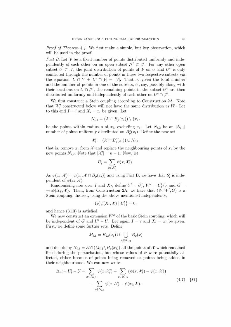
STEIN COUPLINGS FOR NORMAL APPROXIMATION 35
Proof of Theorem 4.4. We first make a simple, but key observation, whichwill be used in the proof:
Fact B. Let Y be a fixed number of points distributed uniformly and inde-pendently of each other on an open subset J ′ ⊂ J . For any other opensubset U ⊂ J , the joint distribution of points of Y on U and U c is onlyconnected through the number of points in these two respective subsets viathe equation |U ∩ Y| + |U c ∩ Y| = |Y|. That is, given the total numberand the number of points in one of the subsets, U , say, possibly along withtheir locations on U ∩ J ′, the remaining points in the subset U c are thendistributed uniformly and independently of each other on U c ∩ J ′.
We first construct a Stein coupling according to Construction 2A. Notethat W ′
i constructed below will not have the same distribution as W . Letto this end I = i and Xi = xi be given. Let
Ni,1 =(
X ∩Bρ(xi))
\ xibe the points within radius ρ of xi, excluding xi. Let Ni,2 be an |Ni,1|number of points uniformly distributed on Bc
ρ(xi). Define the new set
X ′i =
(
X ∩Bcρ(xi)
)
∪Ni,2;
that is, remove xi from X and replace the neighbouring points of xi by thenew points Ni,2. Note that |X ′
i | = n− 1. Now, let
U ′i =
∑
x∈X ′i
ψ(x,X ′i ).
As ψ(xi,X ) = ψ(xi,X ∩Bρ(xi)) and using Fact B, we have that S′i is inde-
pendent of ψ(xi,X ).Randomising now over I and XI , define U
′ = U ′I , W
′ = U ′I/σ and G =
−nψ(XI ,X ). Then, from Construction 2A, we have that (W,W ′, G) is aStein coupling. Indeed, using the above mentioned independence,Eψ(Xi,X )
∣
∣ U ′i
= 0,
and hence (3.13) is satisfied.We now construct an extensionW ′′ of the basic Stein coupling, which will
be independent of G and U ′ − U . Let again I = i and Xi = xi be given.First, we define some further sets. Define
Mi,1 = B2ρ(xi) ∪⋃
x∈Ni,2
Bρ(x)
and denote by Ni,3 = X ∩ (Mi,1 \Bρ(xi)) all the points of X which remainedfixed during the perturbation, but whose values of ψ were potentially af-fected, either because of points being removed or points being added intheir neighbourhood. We can now write
∆i := U ′i − U =
∑
x∈Ni,2
ψ(x,X ′i ) +
∑
x∈Ni,3
(
ψ(x,X ′i )− ψ(x,X )
)
−∑
x∈Ni,1
ψ(x,X )− ψ(xi,X ).(4.7) 57

STEIN COUPLINGS FOR NORMAL APPROXIMATION 36
LetMi,2 = B3ρ(xi) ∪
⋃
x∈Ni,2
B2ρ(x).
Clearly, the values of ∆i and ψ(xi,X ) are determined by the points X ∩Mi,2
and X ′ ∩Mi,2 only. Given the points X ∩Mi,2 and X ′ ∩Mi,2, we have fromFact A that the remaining n−|X∩Mi,2| points of X are distributed uniformlyand independently of each other on M c
i,2. Hence we can use them for our
construction ofW ′′ as follows. First, let Ni,4 be a Bi(n,Vol(Mi,2)/n) numberof points distributed independently and uniformly onMi,2. Then, let Ni,5 bethe remaining n− |Ni,4| points on M c
i,2 distributed as follows. Let P (k) bek random points distributed uniformly on M c
i,2 if k > 0, and let, for k < 0,
P (k) be |k| randomly chosen points from X ∩M ci,2 (without replacement);
set P (0) = ∅. Let P := P (|X ∩Mi,2| − |Ni,4|) and define
Ni,5 =
(X ∩M ci,2) \ P if |Ni,4| > |X ∩Mi,2|,
(X ∩M ci,2) ∪ P if |Ni,4| 6 |X ∩Mi,2|;
that is, we let Ni,5 be the points X ∩M ci,2 and add or remove as many points
(that is the points P ) as needed so that |Ni,4| + |Ni,5| = n. Now, settingX ′′i = Ni,4∪Ni,5, we clearly have that U ′′
i =∑
x∈X ′′iψ(x,X ′′
i ) is independent
of (ψ(xi,X ),∆) as the conditional distribution of X ′′i given (X ∩Mi,2,X ′
i ∩Mi,2) always equals to L (X ) by construction and (X ∩ Mi,2,X ′
i ∩ Mi,2)determines (ψ(xi,X ),∆i) as mentioned before. Randomizing over I andXI , set U ′′ = U ′′
I and W ′′ = U ′′/σ. Thus, (W,W ′, G,W ′′) satisfies the
assumptions of Corollary 2.4 when setting D = D. It remains to find thecorresponding quantities A and B.
Define the sets
Mi,3 = B4ρ(xi) ∪⋃
x∈Ni,2
B3ρ(x),
Mi,4 =⋃
x∈P
Bρ(x),
and let
Y1 := |X ∩ (Bρ(xi) \ xi)| = |Ni,1| = |Ni,2|Y2 := |X ∩ (Mi,2 \Bρ(xi))| = |X ∩Mi,2| − 1− Y1,
Y3 := |X ∩ (Mi,3 \Mi,2)| = |X ∩Mi,3| − 1− Y1 − Y2,
Y4 := |Ni,4| = |X ′′i ∩Mi,2|.
Let κρ := Vol(Bρ(0)). Then the following statements are straightforward:
(i) L (Y1) = Bi(n− 1, κρ/n),
(ii) L (Y2 + Y3|Ni,2) = Bi(
n− 1− Y1,Vol(Mi,3\Bρ(xi))
(n−κρ)
)
,
(iii) L (Y4|Ni,2) = Bi(
n,Vol(Mi,2)/n)
,
(iv) Y4 ⊥⊥ (Y2, Y3) given Ni,2,
(v) |P | 6 |X ∩Mi,2|+ |X ′′i ∩Mi,2| = 1 + Y1 + Y2 + Y4,
(vi) |X ′′i ∩Mi,3| 6 Y4 + Y3 + |P | 6 1 + Y1 + Y2 + Y3 + 2Y4,

STEIN COUPLINGS FOR NORMAL APPROXIMATION 37
(vii) |(X ′′i \ P ) ∩Mi,4| 6 |X ′′
i ∩Mi,3|+ Y5 and
|(X \ P ) ∩Mi,4| 6 |Xi ∩Mi,3|+ Y5,
for some Y5 with L (Y5|P,Ni,2, Ni,4) ∼ Bi(
n− Y1 − 1,Vol(Mi,4)
n−Vol(Mi,3)
)
,
The bound in (vi) follows from the fact that the difference between thepoints X ∩ (Mi,3 \Mi,2) and X ′′∩ (Mi,3 \Mi,2) is at most the points from P .The somewhat rough bound (vii) is due to the fact that the neighbourhoodsof the points in P may overlap with Mi,3.
Let now C be a constant that may depend only on the dimension d butcan change from formula to formula. From representation (4.7), we easilyobtain
|Di| 6 ‖ψ‖(
|Ni,2|+ 2|Ni,3|+ |Ni,1|+ 1)
/σ 6 C‖ψ‖(Y1 + Y2 + 1)/σ.
Now, we can write ∆′i := U ′′
i − U as
∆′i =
∑
x∈X ′′i ∩Mi,3
ϕ(x,X ′′i )−
∑
x∈X∩Mi,3
ϕ(x,X )
+∑
x∈X ′′i ∩(Mi,4\Mi,3)
ϕ(x,X ′′i )−
∑
x∈X∩(Mi,4\Mi,3)
ϕ(x,X ),
hence
|D′i| 6 ‖ψ‖
(
|X ′′i ∩Mi,3|+ |X ∩Mi,3|+ |X ′′
i ∩Mi,4|+ |X ∩Mi,4|)
/σ
6 C‖ψ‖Z/σ,
where Z := 1 + Y1 + Y2 + Y3 + Y4 + Y5.To estimate the third absolute moment of Z note first that if Y ∼ Bi(m, p)
with mp > 1 we have EY 3 6 5m3p3.
Note that the assumption ρ > π−1/2Γ(1+d/2)1/d implies that EY1 = κρ > 1
because κρ = ρdκ1 = ρdπd/2/Γ(1 + d/2).As the cubic function is convex on the non-negative half line, we have for
any non-negative numbers a1, . . . , am that
(a1 + · · ·+ am)3 6 m2(a31 + · · ·+ a3m).
From (i) we immediately obtainEY 31 6 5κ3ρ. (4.8) 58
From (ii)–(iv) we have that, given Y1, Y2 + Y3 + Y4 is stochastically domi-nated by Bi(2n, 2Vol(Mi,3)/n) which is further stochastically dominated byBi(2n, (2κ4ρ + 2κ3ρY1)/n), where we define Bi(m, p) := Bi(m, 1) if p > 1;hence, using this and (4.8),E(Y2 + Y3 + Y4)
36 CE(κ4ρ + κ3ρY1)
36 C(κ3ρ + κ6ρ). (4.9) 59
Note now that, given P , Ni,2 and Ni,4, we have from (vii) that L (Y5) isstochastically dominated by Bi(n− 1−Y1, κρ|P |/(n−κ4ρ−κ3ρY1)+) which,

STEIN COUPLINGS FOR NORMAL APPROXIMATION 38
by (v), can be dominated by Bi(n− 1− Y1, κρ(1 + Y1 + Y2 + Y4)/(n− κ4ρ −κ3ρY1)+); hence, using this, (4.8) and (4.9), we obtainEY 3
5 6 CE(n− 1− Y1)
(
1 ∧κ3ρ(1 + Y1 + Y2 + Y4)
(n− κ4ρ − κ3ρY1)+
)3
6 nP[Y1 > cn] + Cκ3ρE(1 + Y1 + Y2 + Y4)3
for n large enough and c such that n− κ4ρ − cnκ3ρ > n/2, e.g. c = 1/(4κ3ρ)and n > 4κ4ρ. From the Chernoff-Hoeffding inequality we obtain thatP[Y1 > cn] 6 2−cn for cn large enough. Hence, nP[Y1 > nc] 6 C 6 Cκ3ρand EY 3
5 6 Cκ3ρ(
1 +EY 31 +E(Y2 + Y3 + Y4)
3)
6 C(κ3ρ + κ6ρ + κ9ρ).(4.10) 60
Putting (4.8)–(4.10) together we obtainEZ3 6 C(1 +EY 31 +E(Y2 + Y3 + Y4)
3 +EY 35 )
6 C(1 + κ3ρ + κ6ρ + κ9ρ) 6 Cκ9ρ,
as κρ > 1. HenceE|D′|3 = 1
n
n∑
i=1
E|D′i|3 6 C‖ψ‖3κ9ρ/σ3 =: A3.
Furthermore, we haveE|G|3 6 n3‖ψ‖3/σ3 =: B3. (4.11) 61Now, Corollary 2.4 yields
dW(
L (W ),N(0, 1))
6 5A2B 6 Cn‖ψ‖3κ6ρ/σ3.By recalling that κρ = ρdκ1 we obtain the final bound.
4.4. Susceptibility and related statistics in the sub-critical Erdos-Renyi random graph. Let H be a graph (here, we use the letter ‘H’ forgraphs as the letter ‘G’ is used in the context of Stein couplings). Then,susceptibility χ(H) is defined to be the expected size of the componentcontaining a uniformly chosen random vertex. That is, if Ci ⊂ H, i =1, . . . ,K are the K maximal subgraphs of the graph H,
χ(H) =K∑
i=1
|Ci|n
|Ci|, (4.12) 62
where |Ci| denotes the number of vertices in subgraph Ci. Using a differentnormalisation in (4.12) we can also write
K∑
i=1
|Ci|n
|Ci|n
=1
nχ(H), (4.13) 63
which, hence, is the probability that, for a given graphH, two randomly cho-sen vertices are in the same component, or, equivalently, connected througha path. Note that, as H is random, the probability of being connected istherefore itself a random quantity.

STEIN COUPLINGS FOR NORMAL APPROXIMATION 39
Using a martingale CLT it was proved by Janson and Luczak (2008) that,if H is a sub-critical Erdos-Renyi graph, χ(H) is asymptotically normal.However, it is well known that standard martingale CLTs will often not yieldoptimal rates of convergence with respect to the Kolmogorov metric (see e.g.Bolthausen (1982)). As often the actual dependence structure under con-sideration is much weaker than in a worst-case scenario, Rinott and Rotar′
(1998) provide bounds that incorporate expressions to measure the depen-dency and which yield optimal bounds in many settings, but the involvedquantities are typically hard to calculate. Let us derive here some boundswithout using martingales and which are optimal up to some additionallogarithmic factors.
Let us consider here more general statistics that depend only on the prop-erties of the components of two randomly chosen vertices. For a vertexi ∈ V (H) denote by C(H, i) ⊂ H the component (i.e. the maximal sub-graph) containing i. Let h = h(H, i, j) be a function that is determined byi and j and the two components that contain i and j, respectively, that is,
h(H, i, j) = h(H ∩ (C(H, i) ∪ C(H, j)), i, j), for all H, i and j, (4.14) 64and which is symmetric in the sense that
h(H, i, j) = h(H, j, i), for all H, i and j. (4.15) 65Then define
U(H) :=∑
i∈V (H)
∑
j∈V (H)
h(H, i, j). (4.16) 66
We can recover susceptibility (4.12) from (4.16) (up to a normalising con-stant) simply by choosing
h(H, i, j) = I[i and j are in the same component]. (4.17) 67As there is little hope for a normal limit for general h we consider functionsthat are non-zero only if the two random vertices are in the same component,that is,
C(H, i) 6= C(H, j) =⇒ h(H, i, j) = 0. (4.18) 68Hence, under (4.18), we can write (4.16) also as
U(H) =∑
i∈V (H)
∑
j∈C(H,i)
h(H, i, j). (4.19) 69
Dependence on just one vertex and its component is, of course, also coveredas a special case h(H, i, i) = h0(H, i) and h(H, i, j) = 0 if i 6= j. For exampleh0(H, i) = I[|C(H, i)| = 1] yields the total number of singletons, or, moregenerally, choose h0(H, i) = I[C(H, i) > m0] to obtain the number of verticesthat are in a component of size larger than m0. We can also recover (4.12)by setting h0(H, i) = |C(H, i)|2/n, however this function is not Lipschitz inthe size of the component. Other quantities of interest may be obtained,such as
h(H, i, j) = I[i and j are connected, but not further than m0 apart],
h(H, i, j) = I[i and j are in the same cycle],
h(H, i, j) = I[i and j are connected]/|C(H, i)|.

STEIN COUPLINGS FOR NORMAL APPROXIMATION 40
Note that by summing uniformly over all the vertices, the components aresize-biased. However, we can ‘de-bias’ as follows: for a given h0(H, i) ofinterest, hu0 (H, i) = h0(H, i)/|C(H, i)| gives the corresponding unbiased re-sult, where now summing is done uniformly among the components. As|C(H, i)| > 1, we have ‖∆hu0‖ 6 ‖∆h0‖. However, averaging is only possi-ble with respect to the expected number of components, that is, hu0(H, i) =
h0(H,i)|C(H,i)|EK , not the actual number, as the function h0(H,i)
|C(H,i)|K does not sat-
isfy (4.19).We have the following theorem.
Theorem 4.5. Let U be as in (4.16) for some function h satisfying (4.14),(4.15) and (4.18). Let W = (U(H) − µ)/σ, where µ = EU(H) and σ2 =VarU(H). Let
‖h‖ = supH
supi,j∈[n]
|h(H, i, j)| > 1
and, with Hk,l denoting the graph where an additional edge is added betweenk and l if k 6= l,
‖∆h‖ = supi,j,k,l∈[n]
supH
∣
∣h(Hk,l, i, j) − h(H, i, j)∣
∣ > 1.
Assume that 0 6 h(H, i, j) 6 2‖∆h‖ whenever H is such that the com-ponents which contain i and j, respectively, are singletons. Let H be anErdos-Renyi random graph with n vertices and edge probabilities λ/n < 1/n.Then, there is a universal constant K > 0 such that
dK(
L (W ),N(0, 1))
6 K
(
n log(n‖h‖)11‖∆h‖3(1 + 1/a2 + σ2/n)
λa11σ3+ea ln(n‖h‖)2
λa2σ2
)
whenever
a := λ− 1− log λ 6 4 ln(n‖h‖). (4.20) 70
Let now λ < 1 be fixed and let h be as in (4.17) to obtain susceptibil-ity (up a normalising constant). Clearly, ‖h‖ = 1 and ‖∆h‖ = 1. FromJanson and Luczak (2008) we have that VarU(H) ∼ 2λn(1 − λ)−5, henceTheorem 4.5 yields a Kolmogorov bound of order log(n)11/
√n.
Proof of Theorem 4.5. We will make use of Construction 2A to obtain aStein coupling. We consider throughout the vertex set [n]. Let CV (H, i)denote the vertices of C(H, i). If e = k, l ⊂ V (H) = [n] is a potentialedge in a graph H on [n] and K ⊂ [n], write e ∼ K if k ∈ K or l ∈ K (orboth). Write e 6∼ K if k /∈ K and l /∈ K.
Let now ξ = (ξi,j), where i, j ∈ [n] and i 6= j, be an i.i.d. family ofBe(λ/n) distributed random variables. Let H be the graph on the vertexset [n] with edge set ξ, that is, e is an edge in H iff ξe = 1. Let H∗ be anindependent copy of H. Note that, given C(H, i), we have that (ξe)e 6∼CV (H,i)
is a family of i.i.d. Be(λ/n) random variables. Define the random graph H ′i
through
e ∈ E(H ′i) : ⇐⇒ e ∈ E(H∗) and e ∼ CV (H, i), or
e ∈ E(H) and e 6∼ CV (H, i).

STEIN COUPLINGS FOR NORMAL APPROXIMATION 41
As H ′i, given C(H, i), is always an unconditional Erdos-Renyi random graph
by construction, we have that C(H, i) is independent of the graph H ′i.
Now, let I be uniformly and independently distributed on [n]. Set H ′ =H ′
I , U = U(H) and U ′ = U(H ′). Furthermore, W = (U − µ)/σ, W ′ =(U ′ − µ)/σ and
G = −nσ
(
∑
j∈C(H,I)
h(H, I, j) − µI
)
,
where µi := E∑
j∈C(H,i) h(H, i, j). Then, it is easy to see that (3.13) is
satisfied and hence we have a Stein coupling.Let now
Vi :=⋃
k∈CV (H,i)
CV (H′i, k)
be all those vertices of the graphH whose components are affected by chang-ing from H to H ′
i; that is, the vertices CV (H, i) themselves on one hand and,on the other hand, the vertices [n] \CV (H, i) that got connected in H ′
i to atleast one of the vertices CV (H, i).
Then we can write
∆i := U(H ′i)− U(H) =
∑
k∈Vi
∑
l∈CV (H,k)
(
h(H ′i, k, l) − h(H, k, l)
)
.
Note that the subgraphs H ∩ Vi and H ′i ∩ Vi determine the value of ∆i.
Hence, similarly as before, let H∗∗ be an independent copy of H and definethe graph H ′′
i by
e ∈ E(H ′′i ) : ⇐⇒ e ∈ E(H∗∗) and e ∼ Vi, or
e ∈ E(H) and e 6∼ Vi.
With the same argument as before, H ′′i is independent of H∩Vi and H ′
i∩Vi.Define
V ′i =
⋃
k∈Vi
CV (H′′i , k)
to be all those vertices of the graph H whose components are affected bychanging from H to H ′′
i . We can write
∆′i := U(H ′′
i )− U(H) =∑
k∈V ′i
∑
l∈CV (H,k)
(
h(H ′′i , k, l) − h(H, k, l)
)
.
We are now in a position to apply Theorem 2.5. As (W,W ′, G) is a Stein
coupling we have r0 = 0. Setting D = D and S = 1 we have r1 = r2 = 0,and by construction of H ′′
i , that r3 = 0.Let C > 0 to be chosen later. From Durrett (2007, p. 38) we have thatP(|C(H, 1)| > k) 6
e−ak
λ. (4.21) 71
Hence, we obtain the simple estimateE|C(H, 1)|2 =
∫ ∞
0P[|C(H, 1)| > √
x ]dx 62
λa2.
Note also that, if j ∈ CV (H, i),
|h(H, i, j)| 6 ‖∆h‖|C(H, i)|.

STEIN COUPLINGS FOR NORMAL APPROXIMATION 42
This yields |µi| 6 ‖∆h‖E|C(H, i)|2 6 ‖∆h‖ 2λa2 . Furthermore, if j ∈ Vi \
CV (H, i), then
|C(H, j)| 6 |C(H ′i, j)|.
With α := nσ‖∆h‖(C2 + 2
λa2) we haveP[|G| > α] 6 P[|C(H, I)| > C] +P[|G| > α, |C(H, I)| 6 C]
and, noticing that the last term is zero, this is
= P[|C(H, 1)| > C].
Furthermore, with β := 2C4‖∆h‖/σ,P[|D| > β]
6 P[|C(H, I)| > C] +P[|D| > β, |C(H, I)| 6 C]
6 P[|C(H, 1)| > C]
+P[|C(H, I)| 6 C,∃j ∈ CV (H, I) s.t. |C(H ′I , j)| > C]
+P[|D| > β, |C(H, I)| 6 C, |C(H ′I , j)| 6 C for all j ∈ CV (H, I)]
and, noticing that the last term is zero, this is
6 P[|C(H, 1)| > C] + CP[|C(H, 1)| > C]
= (C + 1)P[|C(H, I)| > C]
Finally, with β′ = 2C5‖∆h‖/σ,P[|D′| > β′]
6 P[|C(H, I)| > C] +P[|D′| > β′, |C(H, I)| 6 C]
6 P[|C(H, 1)| > C]
+P[|C(H, I)| 6 C,∃j ∈ CV (H, I) s.t. |C(H ′I , j)| > C]
+P[|D′| > β′, |C(H, I)| 6 C, |C(H ′I , j)| 6 C ∀j ∈ CV (H, I)]
6 P[|C(H, 1)| > C] + CP[|C(H, 1)| > C]
+P[|C(H, I)| 6 C, |C(H ′I , j)| 6 C ∀j ∈ CV (H, I),
∃j ∈ VI s.t. |C(H ′′I , j)| > C
]
+P[|D′| > β′, |C(H, I)| 6 C, |C(H ′I , j)| 6 C ∀j ∈ CV (H, I),
|C(H ′′I , j)| 6 C ∀j ∈ VI
]
and, noticing that the last term is zero, this is
6 P[|C(H, 1)| > C] + CP[|C(H, 1)| > C] + C2P[|C(H, 1)| > C]
6 (C + 1)2P[|C(H, 1)| > C].
We also have the rough bounds
|G|, |D| 6 2n2
σ‖h‖,

STEIN COUPLINGS FOR NORMAL APPROXIMATION 43
Hence, choosing C = 8 ln(n‖h‖)/a − 1 we have that C > 1 from (4.20),and using (4.21) we haveP[|G| > α] 6
e−aC
λ6
ea
λn4‖h‖2 ,P[|D| > β] 6 (C + 1)e−aC
λ6
4ea ln(n‖h‖)aλn4‖h‖2 ,P[|D′| > β′] 6 (C + 1)2
e−aC
λ6
16ea ln(n‖h‖)2a2λn4‖h‖2 .
From Theorem 2.5 we hence have
dK(L (W ),N(0, 1))
6 12(αβ + 1)β′ + 8αβ2
+4n4‖h‖2σ2
(P[|G| > α] +P[|D| > β] +P[|D′| > β′])
6 12
(
n‖∆h‖σ
(
C2 +2
λa2
)
2C4‖∆h‖σ
+ 1
)
2C5‖∆h‖σ
+ 8n‖∆h‖σ
(
C2 +2
λa2
)
4C8‖∆h‖2σ2
+4n4‖h‖2σ2
(
e2
λn4‖h‖2 +4ea ln(n‖h‖)aλn4‖h‖2 +
16ea ln(n‖h‖)2a2λn4‖h‖2
)
6 24
((
C2 +2
λa2
)
C4 +σ2
n
)
nC5‖∆h‖3σ3
+ 32
(
C2 +2
λa2
)
C8n‖∆h‖3σ3
+84ea ln(n‖h‖)2
a2λσ2
6 32
(
2 +4
a2λ+σ2
n
)
nC11‖∆h‖3σ3
+84ea ln(n‖h‖)2
λa2σ2.
Remark 4.2. Note that (H,H ′i) does not form an exchangeable pair, al-
though the marginal distributions are the same. To see this, denote by Gc
the complete graph and by G0 the empty graph on the vertices [n], wherewe assume n > 2. Now, given H = Gc, H
′i is just an independent realisation
of the Erdos-Renyi random graph, henceP[H ′i = G0|H = Gc] = P[H ′
i = G0] = (1− p)(n2).
On the other hand,P[H = G0|H ′i = Gc] =
P[H ′i = Gc|H = G0]P[H = G0]P[H ′
i = Gc]= 0
since it is not possible that H ′i is a complete graph if H is empty.
5. Zero bias transformation
Assume thatEW = 0 and VarW = 1. It was proved in Goldstein and Reinert(1997) that there exists a unique distribution L (W z) such that, for all

STEIN COUPLINGS FOR NORMAL APPROXIMATION 44
smooth f we have EWf(W )
= Ef ′(W z) (5.1) 72Furthermore, L (W z) has a density ρ with respect to the Lebesgue measure.Let us first discuss the connection between our general framework and ρ.
Lemma 5.1. Let (W,W ′, G) be a Stein coupling. Then, with K(t) asin (2.6),EG(I[W 6 u < W ′]− I[W ′ 6 u < W ])
= EK(u−W ) = ρ(u) (5.2) 73
for Lebesgue almost all u ∈ R.
Proof. The first equality is clear. To prove the second one, let f be abounded Lipschitz-continuous function. We have
Gf(W ′)−Gf(W ) =
∫R f ′(W + t)K(t)dt =
∫R f ′(u)K(u−W )du,
so that, from (1.8) and using Fubini’s Theorem,EWf(W ) =
∫R f ′(u)EK(u−W )du. (5.3) 74
As we may take f(x) = δ−1∫ δ0 I[x 6 a] 6 1 and thus f ′(x) = δ−1I[a 6 x 6
a+ δ] for any a ∈ R and δ > 0, we have from (5.1) and (5.3) that∫ a+δ
aEK(u−W )du =
∫ a+δ
aρ(u)du
which proves the claim as a and δ are arbitrary.
In Goldstein and Reinert (1997) and Goldstein and Reinert (2005b) amethod was introduced to construct L (W z) using an underlying exchange-able pair satisfying the linearity condition (3.2) with R = 0. Although theconstruction itself does not directly lead to a coupling ofW z withW (whichis what we ultimately want), it can nevertheless suggest ways to find suchcouplings; see for example Goldstein (2005) and Ghosh (2009).
We can generalize the idea to our setting. However, as some of the in-volved measures may become signed measures, we have to proceed with morecare. Denote by F the probability measure on R2 induced by (W,W ′). With
ϕ(w,w′) := E(GD |W = w,W = w′) = (w′ − w)E(G |W = w,W = w′)
define a new (possibly signed) measure
dF (w,w′) = ϕ(w,w′)dF (w,w′).
We have∫R2 dF (w,w′) = 1 because E(GD) = 1 from (1.8). Let now the
space Ω := R2 × [0, 1] be equipped with the standard Borel σ-algebra and
define the measure Q = F ⊗ ℓ where ℓ is the Lebesgue measure on [0, 1].
Define the mapping W z : Ω → R as
W z(w,w′, u) := uw′ + (1− u)w
Clearly, W z is measurable. We now have the following.

STEIN COUPLINGS FOR NORMAL APPROXIMATION 45
Lemma 5.2. Assume that (1.8) holds. Then, the measure P z on R inducedby the mapping W z is a probability measure and for every function f : R→R with bounded derivative we haveEWf(W )
=
∫
Ωf ′(W z(w,w′, u))dQ(w,w′, u) =
∫R f ′(x)ρ(x)dx. (5.4) 75
Proof. Let us proof the first equality of (5.4).∫
Ωf ′(W z(w,w′, u))dQ(w,w′ , u)
=
∫R2
∫
[0,1]f ′(w + u(w′ − w))du dF (w,w′)
=
∫R2
f(w′)− f(w)
w′ − wdF (w,w′)
=
∫R2
ϕ(w,w′)f(w′)− f(w)
w′ − wdF (w,w′)
= EG(f(W ′)− f(W )) = EWf(W ).We thus have proved that the measure P z, induced by W z and Q, satisfiesEWf(W ) =
∫R f ′(x)dP z(x). (5.5) 76
Using the special functions from the proof of Lemma 5.1, it is clear from(5.5) and (5.1) that ρ is the Radon-Nykodim derivative of P z with respectto the Lebesgue measure. This implies the second equality in (5.4).
In the case where ϕ(W,W ′) > 0 almost surely, F is also a probabilitymeasure and we can write
W z = UW ′ + (1− U)W
where (W,W ′) has distribution F and U ∼ U [0, 1] is independent of (W,W ′).
6. Proofs of main results
6.1. Preliminaries. For a random variable X define the truncated versionX := (X ∧ 1) ∨ (−1). For a real number t define t+ = t ∨ 0 and t− = t ∧ 0.
Stein’s method for normal approximation is based on the differential equa-tion
f ′(w)− wf(w) = h(w) −Eh(Z) (6.1) 77where Z ∼ N(0, 1) which can be solved for any measurable function h forwhich Eh(Z) exists. The solution fh is differentiable and, if h is Lipschitz,also f ′h is Lipschitz; see Stein (1986).
Lemma 6.1. Let W , W ′, W ′′, D and G be square integrable random vari-ables. Let h be a measurable function for which Eh(W ) and Eh(Z) existand let f be the solution to (6.1). Then∣
∣Eh(W )−Eh(Z)∣∣ 6 (‖f‖∨‖f ′‖)r0+‖f ′‖(r1+r2+r3)+|ER1(f)|+|ER2(f)|,where
R1(f) = (GD − S)(f ′(W ′′)− f ′(W )) (6.2) 78

STEIN COUPLINGS FOR NORMAL APPROXIMATION 46
R2(f) = G
∫ D
0
(
f ′(W + t)− f ′(W ))
. (6.3) 79
Proof. Let f = fh be the solution to (6.1). We can assume that ‖f‖ and ‖f ′‖are finite otherwise the statement is trivial. From the fundamental theoremof calculus, we have
f(W ′)− f(W ) =
∫ D
0f ′(W + t)dt. (6.4) 80
Multiplying (6.4) by G and comparing it with the left hand side of (6.1) wehave
h(W )−Eh(W ) = f ′(W )−Wf(W )
= Gf(W ′)−Gf(W )−Wf(W )
+ (S −GD)f ′(W ′′)
+ (1− S)f ′(W )
+G(D −D)f ′(W )
+ (S −GD)(f ′(W )− f ′(W ′′))
−G
∫ D
0
(
f ′(W + t)− f ′(W ))
dt.
(6.5) 82
Taking expectation, the lemma is immediate.
6.2. Bound on the Wasserstein distance. If h is Lipschitz continuous,then the solution f to (6.1) is differentiable, f ′ is Lipschitz and we have thefollowing bounds:
‖f‖ 6 2‖h′‖, ‖f ′‖ 6
√
2
π‖h′‖, ‖f ′′‖ 6 2‖h′‖. (6.6) 83
(see Stein (1972) and Raic (2004)).
Proof of Theorem 2.1. The following bounds are easy to obtain using Tay-lor’s theorem:
|ER1(f)| 6 2r′4‖f ′‖+ r′5‖f ′′‖, |ER2(f)| 6 2r4‖f ′‖+ 0.5r5‖f ′′‖.Combining this with Lemma 6.1 and the bounds (6.6) for Lipschitz h with‖h′‖ 6 1 proves the theorem.
6.3. Bounds on the Kolmogorov distance. If, for some ε > 0, h is ofthe form
ha,ε(x) =
1, if x 6 a,
1 + (a− x)/ε, if a 6 x 6 a+ ε,
0, if x > a+ ε,
(6.7) 84
then, from pages 23 and 24 of Stein (1986) (see also Chen and Shao (2004))we have for fa,ε for every w, v ∈ R the bounds
0 6 fa,ε(w) 6√2π/4, |f ′a,ε(w)| 6 1, |f ′a,ε(w)− f ′a,ε(v)| 6 1 (6.8) 85
and, in addition for every s, t ∈ R,
|f ′a,ε(w + s)− f ′a,ε(w + t)|

STEIN COUPLINGS FOR NORMAL APPROXIMATION 47
6 (|w| + 1)min(|s|+ |t|, 1) + ε−1
∫ s∨t
s∧tI[a 6 w + u 6 a+ ε]du (6.9) 86
6 (|w| + 1)min(|s|+ |t|, 1) + I[a− s ∨ t 6 w 6 a− s ∧ t+ ε]. (6.10) 87
Throughout this section let κ := dK(
L (W ),N(0, 1))
. Now, it is notdifficult to see that for any ε > 0,
κ 6 supa∈R∣∣Eha,ε(W )−Eha,ε(Z)∣∣+ 0.4ε, (6.11) 90
so that we can use Lemma 6.1 for functions of the form (6.7). If fa,ε is thesolution to (6.1), from the bounds (6.8) we thus have
κ 6 r0 + r1 + r2 + r3 + 0.4ε+ supa∈R |ER1(fa,ε)|+ sup
a∈R |ER2(fa,ε)|, (6.12) 91
which will be the basis for further bounds on κ.Recall the well known relation between the arithmetic and geometric
mean, that is, for each x, y > 0 and θ > 0 we have
√xy 6
θx+ θ−1y
2, (6.13) 92
which will be used several times. We will also make use of the followingsimple lemma in order to implement the recursive approach; see Raic (2003).
Lemma 6.2. For any random variable V and for any a < b we haveP[a 6 V 6 b] 6b− a√2π
+ 2 dK(
L (V ),N(0, 1))
. (6.14) 93
Proof of Theorem 2.5. Let f = fa,ε be the solution to (6.1), where we willfrom now on omit the dependency on a and ε for better readability. LetI1 = I[|G| 6 α, |D| 6 β, |D′| 6 β′, |S| 6 γ] and write (6.2) asER1(f) = E(GD − S)(1 − I1)(f
′(W ′′)− f ′(W ))
+E(GD − S)I1(f′(W ′′)− f ′(W ))
=: J1 + J2.
Using (6.8), the bound |J1| 6 r′6 is immediate. Let for convenience k :=E|W |+ 1. Using (6.9) and Lemma 6.2,
J2 6 E∣∣(GD − S)I1(
f ′(W ′′)− f ′(W ))∣
∣
6 (αβ + γ)kβ′ + (αβ + γ)ε−1
∫ β′
−β′
P[a 6W + u 6 a+ ε]du
6 (αβ + γ)kβ′ + 0.8(αβ + γ)β′ + 4(αβ + γ)β′ε−1κ.
Similarly, let I2 = I[|G| 6 α, |D| 6 β] and write (6.3) asER2(f) = EG(1− I2)
∫ D
0
(
f ′(W + t)− f ′(W ))
dt
+EGI2 ∫ D
0
(
f ′(W + t)− f ′(W ))
dt
=: J3 + J4.

STEIN COUPLINGS FOR NORMAL APPROXIMATION 48
By (6.8), |J3| 6 r6. Using (6.9) and Lemma 6.2,
J4 6 E∣∣∣∣
GI2
∫ D+
D−
∣
∣f ′(W + t)− f ′(W )∣
∣dt
∣
∣
∣
∣
6 α
∫ β
−β|t|kdt+ αε−1
∫ β
−β
∫ t+
t−
P[a 6W + u 6 a+ ε]dudt
6 αβ2k + 0.4αβ2 + 2αβ2ε−1κ,
so that, collecting all the bounds, setting ε = 4αβ2+8(αβ+γ)β′ and makinguse of (6.12), we obtain
κ 6 r0 + r1 + r2 + r3 + r6 + r′6 + (αβ + γ)(k + 0.8)β′ + (k + 0.4)αβ2
+ 0.4ε +(
2αβ2 + 4(αβ + γ)β′)
ε−1κ
= r0 + r1 + r2 + r3 + r6 + r′6 + (αβ + γ)(k + 4)β′ + (k + 2)αβ2 + 0.5κ
which, solving for κ, proves the theorem.
Proof of Theorem 2.8. Let f = fa,ε be the solution to (6.1). As we assumeW ′′ =W , we have R1(f) = 0. Write (6.3) as
R2(f) = E∫ ∞
−∞
(
f ′(W + t)− f ′(W ))
KW (t)dt
= E∫|t|>1
(
f ′(W + t)− f ′(W ))
KW (t)dt
+E∫|t|61
(
f ′(W + t)− f ′(W ))(
KW (t)−K(t))
dt
+E∫|t|61
(
f ′(W + t)− f ′(W ))
K(t)dt
=: J1 + J2 + J3.
Clearly, by (6.8), |J1| 6 r4. Now let us bound J2. By (6.10),
|J2| 6 E∫
|t|61
(
|W |+ 1)
|t||KW (t)−K(t)|dt
+E∫ 1
0I[a− t 6W 6 a+ ε]|KW (t)−K(t)|dt
+E∫ 0
−1I[a 6W 6 a− t+ ε]|KW (t)−K(t)|dt
=: J2,1 + J2,2 + J2,3,
Using (6.13), we have for any θ > 0 that
J2,1 6θ
2E∫
|t|61(|W |+ 1)2|t|dt+ 1
2θE∫
|t|61|t||KW (t)−K(t)|2dt
=θ
2E(|W |+ 1)2 +
1
2θr28.
Let α0 = (E(|W |+ 1)2)1/2 and choose θ = α−10 r8, so that
J2,1 6 α0r8.

STEIN COUPLINGS FOR NORMAL APPROXIMATION 49
Let now δ = 0.4ε + 2κ. Then, from Lemma 6.2, we have for t > 0P[a− t 6W 6 a+ ε] 6 δ + 0.4t. (6.15) 94
Using (6.13),
J2,2 6 E∫ 1
0
[
0.5ε(
δ + 0.4t)−1
I[a− t 6W 6 a+ ε]
+ 0.5ε−1(
δ + 0.4t)(
KW (t)−K(t))2]
dt
6 0.5ε+ 0.5ε−1δ
∫ 1
0Var(KW (t))dt+ 0.2ε−1
∫ 1
0tVar(KW (t))dt.
A similar bound holds for J2,3 so that
|J2| 6 α0r8 + ε+ 0.5ε−1δr7 + 0.2ε−1r28.
By (6.9),
|J3| 6 E∫
|t|61(|W |+ 1)|tK(t)|dt
+ ε−1
∫
|t|61
∣
∣
∣
∣
∫ t
0P[a 6W + u 6 a+ ε]du
∣
∣
∣
∣
|K(t)|dt
6 (E|W |+ 1)r5 + ε−1
∫
|t|61δ|tK(t)|dt 6 (E|W |+ 1)r5 + ε−1δr5.
Choose now
ε =√1.4
[
κ(2r5 + r7) + 0.2r28]1/2
.
From (6.12) (note that r1 = 0 because D = D), using that√x+ y 6√
x+√y and (6.13), we obtain
κ 6 r0 + r2 + r3 + 0.4ε + |J1|+ |J2|+ |J3|6 r0 + r2 + r3 + r4 + (E|W |+ 1)r5 + α0r8 + 1.4ε
+ ε−1(δ(r5 + 0.5r7) + 0.2r28)
6 r0 + r2 + r3 + r4 + (E|W |+ 1.4)r5 + 0.2r7 + α0r8 + 1.4ε
+ ε−1(
κ(2r5 + r7) + 0.2r28)
6 r0 + r2 + r3 + r4 + (E|W |+ 1.4)r5 + 0.2r7 + α0r8
+ 2.4(
κ(2r5 + r7) + 0.2r28)1/2
6 r0 + r2 + r3 + r4 + (E|W |+ 1.4)r5 + 0.2r7 + (α0 + 1.1)r8
+ 2.4(
κ(2r5 + r7))1/2
6 r0 + r2 + r3 + r4 + (E|W |+ 1.4 + 2.4θ−1)r5 + (0.2 + 1.2θ−1)r7
+ (α0 + 1.1)r8 + 1.2θκ
Choosing θ = 1/2.4 and solving for κ proves the claim.

STEIN COUPLINGS FOR NORMAL APPROXIMATION 50
Proof of Theorem 2.9. Let f = fa,ε be the solution to (6.1). Now, from (6.9),
|R1(f)| 6∣
∣(S −GD)(|W |+ 1)D′∣
∣
+ |S −GD|ε−1
∫ D′+
D′−
I[a 6W + u 6 a+ ε]du
so that E|R1(f)| 6 E∣∣(S −GD)(|W |+ 1)D′∣
∣
+ ε−1E∣∣(S −GD)D′Sε(L (W |G, D,D′))∣
∣.
Furthermore,
|R2(f)| 6 |G|∫ D+
D−
(|W |+ 1)(|t| ∧ 1)dt
+ ε−1|G|∫ D+
D−
∫ t+
t−
I[a 6W + u 6 a+ ε]dudt
henceE|R2(f)| 6 0.5E|G(|W | + 1)D2|+ 0.5ε−1E∣∣GD2Sε(L (W |G,D))∣
∣
Combining these bounds with (6.12) proves the theorem.
To prove Lemma 2.10 we first need a simple lemma.
Lemma 6.3. Let βk,l, 1 6 l < k, k = 2, . . . , n, be non-negative real numbers.If a1 6 b1 = 1 and if there are constants q > 1 and p < 1 such that, for all
k = 2, 3, . . . , n, we have∑k−1
l=1 βk,l 6 p,
ak = q +k−1∑
l=1
βk,lal and bk = q + pbk−1,
then ak 6 bk 6 q/(1− p) for all 1 6 k 6 n.
Proof. Note first that q/(1− p) > 1 and
bk =
(
1− q
1− p
)
pk +q
1− p,
hence b1, b2, . . . is increasing with upper bound q/(1 − p). The proof ofak 6 bk is now a simple induction on k. By assumption a1 6 b1, whichverifies the base case. Using that al 6 bl for all 1 6 l 6 k, we have
ak+1 = q +
k∑
l=1
βk+1,lal 6 q +
k∑
l=1
βk+1,lbl
6 q +
k∑
l=1
βk+1,lbk 6 q + pbk = bk+1.
Proof of Lemma 2.10. First note that (2.8) still holds if we replace A byA := A∨1. Let σ1 := 1 and define a new sequence ak = σkκk for 1 6 k 6 n.

STEIN COUPLINGS FOR NORMAL APPROXIMATION 51
Using inequality (2.8) with ε = cnαn/σk for a constant cn > 1 to be chosenlater,
ak 6 A+ 0.4cnαn +
k−1∑
l=1
βk,lal
for all 1 6 k 6 n, where
βk,l =σkAk,l
cnσlαn.
Note that∑k−1
l=1 βk,l 6 c−1n . Consider now the solution bk to the recursive
equation
b1 = 1; bk = A+ 0.4cnαn + c−1n bk−1, for 2 6 k 6 n.
Note that A+ 0.4cnαn > 1, hence we obtain from Lemma 6.3 that
an 6 bn 6cn(A+ 0.4cnαn)
cn − 1.
Minimizing over cn > 1 we can chose
cn = 1 +
√
2αn(2αn + 5A))
2αn= 1 +
α′n
2αn.
Recalling that κn = an/σn, the claim follows.
Acknowledgments
The authors would like to thank Andrew Barbour, Omar El-Dakkak,Larry Goldstein, Erol Pekoz and Nathan Ross for helpful discussions.
References
P. Baldi, Y. Rinott, and C. Stein (1989). A normal approximation for thenumber of local maxima of a random function on a graph. In Probability,statistics, and mathematics, pages 59–81. Academic Press, Boston, MA.
A. D. Barbour (1988). Stein’s method and Poisson process convergence.J. Appl. Probab. 25A, 175–184.
A. D. Barbour (2009). Univariate approximations in the infinite occupancyscheme. ALEA 6, 415—433.
A. D. Barbour and G. K. Eagleson (1986). Random association of symmetricarrays. Stochastic Anal. Appl. 4, 239–281.
A. D. Barbour, M. Karonski, and A. Rucinski (1989). A central limit the-orem for decomposable random variables with applications to randomgraphs. J. Combin. Theory Ser. B 47, 125–145.
A. D. Barbour, L. Holst, and S. Janson (1992). Poisson approximation,volume 2 of Oxford Studies in Probability. The Clarendon Press OxfordUniversity Press, New York. ISBN 0-19-852235-5. Oxford Science Publi-cations.
H. Bergstrom (1944). On the central limit theorem. Skand. Aktuarietidskr.27, 139–153.
E. Bolthausen (1982). Exact convergence rates in some martingale centrallimit theorems. Ann. Probab. 10, 672–688.
E. Bolthausen (1984). An estimate of the remainder in a combinatorialcentral limit theorem. Z. Wahrsch. Verw. Gebiete 66, 379–386.

STEIN COUPLINGS FOR NORMAL APPROXIMATION 52
M. V. Boutsikas and M. V. Koutras (2002). On the number of overflownurns and excess balls in an allocation model with limited urn capacity. J.Statist. Plann. Inference 104, 259–286.
T. Cacoullos, V. Papathanasiou, and S. A. Utev (1994). Variational inequal-ities with examples and an application to the central limit theorem. Ann.Probab. 22, 1607–1618.
S. Chatterjee (2005). Concentration inequalities with exchangeable pairs.PhD thesis, Stanford University.
S. Chatterjee (2007). Stein’s method for concentration inequalities. Probab.Theory Related Fields 138, 305–321.
S. Chatterjee (2008). A new method of normal approximation. Ann. Probab.36, 1584–1610.
S. Chatterjee (2009). Fluctuations of eigenvalues and second order poincarinequalities. Probab. Theory Related Fields 143, 1–40.
S. Chatterjee, J. Fulman, and A. Rollin (2006). Exponential approximationby exchangeable pairs and spectral graph theory. Preprint. Available athttp://arxiv.org/abs/math/0605552.
L. H. Y. Chen (1975). Poisson approximation for dependent trials. Ann.Probability 3, 534–545.
L. H. Y. Chen (1998). Stein’s method: some perspectives with applications.In Probability towards 2000 (New York, 1995), volume 128 of LectureNotes in Statist., pages 97–122. Springer, New York.
L. H. Y. Chen and Q.-M. Shao (2001). A non-uniform Berry-Esseen boundvia Stein’s method. Probab. Theory Related Fields 120, 236–254.
L. H. Y. Chen and Q.-M. Shao (2004). Normal approximation under localdependence. Ann. Probab. 32, 1985–2028.
L. H. Y. Chen and Q.-M. Shao (2005). Stein’s method for normal approx-imation. In An introduction to Stein’s method, volume 4 of Lect. NotesSer. Inst. Math. Sci. Natl. Univ. Singap., pages 1–59. Singapore Univ.Press, Singapore.
A. Dembo and Y. Rinott (1996). Some examples of normal approximationsby Stein’s method. In Random discrete structures (Minneapolis, MN,1993), volume 76 of IMA Vol. Math. Appl., pages 25–44. Springer, NewYork.
P. Diaconis (1977). The distribution of leading digits and uniform distribu-tion mod 1. Ann. Probability 5, 72–81.
P. Diaconis and S. Zabell (1991). Closed form summation for classical dis-tributions: variations on a theme of de Moivre. Statist. Sci. 6, 284–302.
R. Durrett (2007). Random graph dynamics. Cambridge Series in Statisticaland Probabilistic Mathematics. Cambridge University Press, Cambridge.ISBN 978-0-521-86656-9; 0-521-86656-1.
G. Englund (1981). A remainder term estimate for the normal approxima-tion in classical occupancy. Ann. Probab. 9, 684–692.
J. Fulman (2004a). Stein’s method and non-reversible Markov chains. InStein’s method: expository lectures and applications, volume 46 of IMSLecture Notes Monogr. Ser., pages 69–77. Inst. Math. Statist., Beachwood,OH.

STEIN COUPLINGS FOR NORMAL APPROXIMATION 53
J. Fulman (2004b). Stein’s method, Jack measure, and the Metropolis algo-rithm. J. Combin. Theory Ser. A 108, 275–296.
S. Ghosh (2009). Lp bounds for a combinatorial central limit theorem withinvolutions. Preprint.
S. Ghosh (2010). Multivariate concentration of measure type resultsusing exchangeable pairs and size biasing. Preprint. Available atarXiv:1001.1396v1.
A. L. Gibbs and F. E. Su (2002). On choosing and bounding probabil-ity metrics. International Statistical Review / Revue Internationale deStatistique 70, 419–435.
L. Goldstein (2005). Berry-Esseen bounds for combinatorial central limittheorems and pattern occurrences, using zero and size biasing. J. Appl.Probab. 42, 661–683.
L. Goldstein (2010). A Berry-Esseen bound with applicationsto counts in the Erdos-Renyi random graph. Available athttp://arxiv.org/abs/1005.4390.
L. Goldstein and M. D. Penrose (to appear). Normal approximation forcoverage models over binomial point processes. Ann. Appl. Probab.
L. Goldstein and G. Reinert (1997). Stein’s method and the zero biastransformation with application to simple random sampling. Ann. Appl.Probab. 7, 935–952.
L. Goldstein and G. Reinert (2005a). Distributional transformations, or-thogonal polynomials, and Stein characterizations. J. Theoret. Probab.18, 237–260.
L. Goldstein and G. Reinert (2005b). Zero biasing in one and higher dimen-sions, and applications. In Stein’s method and applications, volume 5 ofLect. Notes Ser. Inst. Math. Sci. Natl. Univ. Singap., pages 1–18. Singa-pore Univ. Press.
L. Goldstein and Y. Rinott (1996). Multivariate normal approximations byStein’s method and size bias couplings. J. Appl. Probab. 33, 1–17.
F. Gotze (1991). On the rate of convergence in the multivariate CLT. Ann.Probab. 19, 724–739.
S. T. Ho and L. H. Y. Chen (1978). An Lp bound for the remainder in acombinatorial central limit theorem. Ann. Probability 6, 231–249.
H.-K. Hwang and S. Janson (2008). Local limit theorems for finite andinfinite urn models. Ann. Probab. 36, 992–1022.
S. Janson and M. J. Luczak (2008). Susceptibility in subcritical randomgraphs. J. Math. Phys. 49, 125207, 23.
N. L. Johnson and S. Kotz (1977). Urn models and their application. JohnWiley & Sons, New York-London-Sydney. An approach to modern dis-crete probability theory, Wiley Series in Probability and MathematicalStatistics.
V. F. Kolchin, B. A. Sevast′yanov, and V. P. Chistyakov (1978). Randomallocations. V. H. Winston & Sons, Washington, D.C.
W. Y. Loh (1975). On the normal approximation for sums of mixing randomvariables. Master’s thesis, University of Singapore.
H. M. Luk (1994). Stein’s method for the gamma distribution and relatedstatistical applications. PhD thesis, University of Southern California.

STEIN COUPLINGS FOR NORMAL APPROXIMATION 54
A. M. Makowski and A. Shwartz (1994). On the Poisson equation for count-able Markov chains: existence of solutions and parameter dependence byprobabilistic methods. Technical report, Institute for Systems Research.
E. Meckes (2008). Linear functions on the classical matrix groups. Trans.Amer. Math. Soc. 360, 5355–5366.
I. Nourdin and G. Peccati (2009). Stein’s method on wiener chaos. Probab.Theory Related Fields.
I. Nourdin, G. Peccati, and G. Reinert (2009). Second order Poincare in-equalities and CLTs on Wiener space. J. of Funct. Anal. 257, 593–609.
M. D. Penrose and J. E. Yukich (2001). Central limit theorems for somegraphs in computational geometry. Ann. Appl. Probab. 11, 1005–1041.
M. Raic (2003). Normal approximation with Stein’s method. In Proceedingsof the Seventh Young Statisticians Meeting.
M. Raic (2004). A multivariate CLT for decomposable random vectors withfinite second moments. J. Theoret. Probab. 17, 573–603.
G. Reinert (1998). Couplings for normal approximations with Stein’smethod. In Microsurveys in discrete probability (Princeton, NJ, 1997),volume 41 of DIMACS Ser. Discrete Math. Theoret. Comput. Sci., pages193–207. Amer. Math. Soc., Providence, RI.
G. Reinert and A. Rollin (2009a). Multivariate normal approximation withStein’s method of exchangeable pairs under a general linearity condition.Ann. Probab. 37, 2150–2173.
G. Reinert and A. Rollin (2009b). U -statistics and random subgraph counts:Multivariate normal approximation via exchangeable pairs and embed-ding. Preprint. Available at arXiv:0912.3425v1.
I. Rinott and V. I. Rotar′ (1998). Some estimates for the rate of convergencein the CLT for martingales. I. Theory Probab. Appl. 43, 604–619.
Y. Rinott and V. Rotar′ (1997). On coupling constructions and rates in theCLT for dependent summands with applications to the antivoter modeland weighted U -statistics. Ann. Appl. Probab. 7, 1080–1105.
Y. Rinott and V. Rotar′ (2000). Normal approximations by Stein’s method.Decis. Econ. Finance 23, 15–29.
A. Rollin (2007a). On Stein factors and the construction of examples withsharp rates in Stein’s method. Preprint.
A. Rollin (2007b). Translated Poisson approximation using exchangeablepair couplings. Ann. Appl. Probab. 17, 1596–1614.
A. Rollin (2008a). A note on the exchangeability condition in Stein’s method.Statist. Probab. Lett. 78, 1800–1806.
A. Rollin (2008b). Symmetric binomial approximation for sums of locallydependent random variables. Electron. J. Probab. 13, 756–776.
N. Ross (to appear). Step size in Stein’s method of exchangeable pairs.Combinatorics, Probability, and Computing.
Q.-M. Shao (2005). An explicit Berry-Esseen bound for Student’s t-statisticvia Stein’s method. 5, 143–155.
Q.-M. Shao and Z.-G. Su (2006). The Berry-Esseen bound for characterratios. Proc. Amer. Math. Soc. 134, 2153–2159 (electronic).
C. Stein (1972). A bound for the error in the normal approximation to thedistribution of a sum of dependent random variables. In Proceedings of

STEIN COUPLINGS FOR NORMAL APPROXIMATION 55
the Sixth Berkeley Symposium on Mathematical Statistics and Probabil-ity (Univ. California, Berkeley, Calif., 1970/1971), Vol. II: Probabilitytheory, pages 583–602, Berkeley, Calif. Univ. California Press.
C. Stein (1986). Approximate computation of expectations. Institute ofMathematical Statistics Lecture Notes—Monograph Series, 7. Institute ofMathematical Statistics, Hayward, CA.
C. Stein (1995). The accuracy of the normal approximation to the distri-bution of the traces of powers of random orthogonal matrices. TechnicalReport No. 470, Standford University Department of Statistics.
J. Sunklodas (2008). On L1 bounds for asymptotic normality of some weaklydependent random variables. Acta Appl. Math. 102, 87–98.
L. Zhao, Z. Bai, C.-C. Chao, and W.-Q. Liang (1997). Error bound ina central limit theorem of double-indexed permutation statistics. Ann.Statist. 25, 2210–2227.
Copyright © 2022 FDOKUMEN