
Approximation Algorithms
232
Approximation Algorithms for Model-Based Diagnosis Aleksandar Feldman
-
Upload
khangminh22 -
Category
Documents
-
view
3 -
download
0
Transcript of Approximation Algorithms
Approximation Algorithmsfor Model-Based Diagnosis
Aleksandar Feldman


Approximation Algorithmsfor Model-Based Diagnosis

Approximation Algorithmsfor Model-Based Diagnosis
PROEFSCHRIFT
ter verkrijging van de graad van doctor
aan de Technische Universiteit Delft,
op gezag van de Rector Magnificus Prof.ir. K.C.A.M. Luyben,
voorzitter van het College voor Promoties,
in het openbaar te verdedigen
op maandag 17 mei 2010 om 15.00 uur
door
Aleksandar Beniaminov FELDMAN
informatica ingenieurgeboren te Varna, Bulgarije.
Dit proefschrift is goedgekeurd door de promotor:
Prof.dr.ir. A.J.C. van Gemund
Samenstelling promotiecommissie:
Rector Magnificus voorzitterProf.dr.ir. A.J.C. van Gemund Technische Universiteit Delft, promotorProf.dr. G. Provan University College CorkProf.dr. C. Witteveen Technische Universiteit DelftProf.dr.ir. H.J. Sips Technische Universiteit DelftProf.dr. K.G. Langendoen Technische Universiteit DelftDr. J. de Kleer Palo Alto Research CenterDr. P.J.F. Lucas Radboud Universiteit Nijmegen
This research was supported by PROGRESS, the embedded systems researchprogram of the Dutch organization for Scientific Research NWO, the DutchMinistry of Economic Affairs and the Technology Foundation STW under awardDES.07015.
Copyright c© 2010 by A. Feldman
All rights reserved. No part of the material protected by this copyright noticemay be reproduced or utilized in any form or by any means, electronic ormechanical, including photocopying, recording or by any information storageand retrieval system, without the prior permission of the author.
isbn 978-90-9025023-6
Cover: Astronaut Andrew Feustel practices installing the Fastener Capture Plateon an underwater mockup of the Advanced Camera for Surveys at the NeutralBuoyancy Laboratory in Houston. Photo used with permission of NASA.
Printed by Wohrmann Print Service, Loskade 4, 7202 CZ Zutphen
Author email: [email protected]

Dedication
To my father Beniamin Feldman (1939 – 2008).

Contents
1 Introduction 1
1.1 Model-Based Diagnosis . . . . . . . . . . . . . . . . . . . . . . . . . 3
1.2 Problem Statement . . . . . . . . . . . . . . . . . . . . . . . . . . . 5
1.3 Contribution . . . . . . . . . . . . . . . . . . . . . . . . . . . . . . 71.3.1 Theory . . . . . . . . . . . . . . . . . . . . . . . . . . . . . 71.3.2 Application . . . . . . . . . . . . . . . . . . . . . . . . . . . 8
1.4 Thesis Outline . . . . . . . . . . . . . . . . . . . . . . . . . . . . . 9
1.5 Origin of Chapters . . . . . . . . . . . . . . . . . . . . . . . . . . . 10
2 Model-Based Diagnosis 13
2.1 Concepts and Definitions . . . . . . . . . . . . . . . . . . . . . . . 132.1.1 A Running Example . . . . . . . . . . . . . . . . . . . . . . 142.1.2 Diagnosis and Minimal Diagnosis . . . . . . . . . . . . . . . 15
2.2 Diagnostic Model Taxonomy . . . . . . . . . . . . . . . . . . . . . 17
2.3 Converting Propositional Formulae to Clausal Form . . . . . . . . 19
2.4 Benchmarks . . . . . . . . . . . . . . . . . . . . . . . . . . . . . . . 20
2.5 Diagnostic Metrics . . . . . . . . . . . . . . . . . . . . . . . . . . . 212.5.1 Classification Errors and Isolation Accuracy . . . . . . . . . 212.5.2 Utilities . . . . . . . . . . . . . . . . . . . . . . . . . . . . . 232.5.3 Consistency . . . . . . . . . . . . . . . . . . . . . . . . . . . 262.5.4 Computational Metrics . . . . . . . . . . . . . . . . . . . . 272.5.5 System Metrics . . . . . . . . . . . . . . . . . . . . . . . . . 28
3 Greedy Stochastic Search for Minimal Diagnoses 29
3.1 Introduction . . . . . . . . . . . . . . . . . . . . . . . . . . . . . . . 29
3.2 Related Work . . . . . . . . . . . . . . . . . . . . . . . . . . . . . . 30
i
ii CONTENTS
3.3 Complexity of Diagnostic Inference . . . . . . . . . . . . . . . . . . 33
3.4 Stochastic MBD Algorithm . . . . . . . . . . . . . . . . . . . . . . 343.4.1 A Simple Example (Continued) . . . . . . . . . . . . . . . . 343.4.2 A Greedy Stochastic Algorithm . . . . . . . . . . . . . . . . 373.4.3 Basic Properties of the Greedy Stochastic Search . . . . . . 403.4.4 Complexity of Inference Using Greedy Stochastic Search . . 43
3.5 Optimality Analysis (Single Diagnosis) . . . . . . . . . . . . . . . . 443.5.1 Optimality of Safari in Weak-Fault Models . . . . . . . . 443.5.2 Optimality of Safari in Strong-Fault Models . . . . . . . . 483.5.3 Validation . . . . . . . . . . . . . . . . . . . . . . . . . . . . 53
3.6 Optimality Analysis (Multiple Diagnoses) . . . . . . . . . . . . . . 55
3.7 Experimental Results . . . . . . . . . . . . . . . . . . . . . . . . . . 603.7.1 Implementation Notes and Test Set Description . . . . . . . 603.7.2 Comparison to Complete Algorithms . . . . . . . . . . . . . 623.7.3 Comparison to Algorithms Based on Max-SAT . . . . . . . 653.7.4 Comparison to Algorithms Based on ALLSAT and Model
Counting . . . . . . . . . . . . . . . . . . . . . . . . . . . . 713.7.5 Performance of the Greedy Stochastic Search . . . . . . . . 733.7.6 Optimality of the Greedy Stochastic Search . . . . . . . . . 743.7.7 Computing Multiple Minimal-Cardinality Diagnoses . . . . 753.7.8 Experimentation Summary . . . . . . . . . . . . . . . . . . 76
3.8 Summary . . . . . . . . . . . . . . . . . . . . . . . . . . . . . . . . 76
4 Computing Worst-Case Diagnostic Scenarios 77
4.1 Introduction . . . . . . . . . . . . . . . . . . . . . . . . . . . . . . . 77
4.2 A Range of MBD Problems . . . . . . . . . . . . . . . . . . . . . . 784.2.1 Observation Vector Optimization Problems . . . . . . . . . 794.2.2 MFMC Properties . . . . . . . . . . . . . . . . . . . . . . . 80
4.3 Worst-Case Complexity . . . . . . . . . . . . . . . . . . . . . . . . 81
4.4 System Description Simplifications . . . . . . . . . . . . . . . . . . 83
4.5 MFMC Algorithm . . . . . . . . . . . . . . . . . . . . . . . . . . . 86
4.6 Experimental Results . . . . . . . . . . . . . . . . . . . . . . . . . . 894.6.1 Experimental Setup, Simplification Results and Bounds . . 894.6.2 Computing MFMC Numbers and Vectors . . . . . . . . . . 90
4.7 Summary . . . . . . . . . . . . . . . . . . . . . . . . . . . . . . . . 94
5 An Active Testing Approach to Sequential Diagnosis 97
5.1 Introduction . . . . . . . . . . . . . . . . . . . . . . . . . . . . . . . 98
5.2 Related Work . . . . . . . . . . . . . . . . . . . . . . . . . . . . . . 100
5.3 Concepts and Definitions . . . . . . . . . . . . . . . . . . . . . . . 1025.3.1 Running Example . . . . . . . . . . . . . . . . . . . . . . . 103
CONTENTS iii
5.3.2 Sequential Diagnosis . . . . . . . . . . . . . . . . . . . . . . 104
5.4 Computing the Expected Number of MC Diagnoses . . . . . . . . 1045.4.1 Computing the Expectation Using Importance Sampling . . 106
5.5 Algorithms for Reducing the Diagnostic Uncertainty . . . . . . . . 1075.5.1 Problem Definition and Exhaustive Search . . . . . . . . . . 1075.5.2 FractalA . . . . . . . . . . . . . . . . . . . . . . . . . . . 1095.5.3 FractalG . . . . . . . . . . . . . . . . . . . . . . . . . . . 1125.5.4 FractalP . . . . . . . . . . . . . . . . . . . . . . . . . . . 114
5.6 Experimental Results . . . . . . . . . . . . . . . . . . . . . . . . . . 116
5.6.1 Experimental Setup . . . . . . . . . . . . . . . . . . . . . . 1165.6.2 Expected Number of MC Diagnoses . . . . . . . . . . . . . 1175.6.3 Comparison of Algorithms . . . . . . . . . . . . . . . . . . . 1195.6.4 Experimental Summary . . . . . . . . . . . . . . . . . . . . 126
5.7 Summary . . . . . . . . . . . . . . . . . . . . . . . . . . . . . . . . 128
6 Conclusions 131
6.1 Contributions . . . . . . . . . . . . . . . . . . . . . . . . . . . . . . 131
6.2 Improvements and Future Work . . . . . . . . . . . . . . . . . . . . 134
A The LYDIA Modeling Language 139
A.1 Systems and Subsystems . . . . . . . . . . . . . . . . . . . . . . . . 139
A.2 Basic Expressions . . . . . . . . . . . . . . . . . . . . . . . . . . . . 142
A.3 Data Types . . . . . . . . . . . . . . . . . . . . . . . . . . . . . . . 142A.3.1 Atomic Data Types . . . . . . . . . . . . . . . . . . . . . . 143A.3.2 Composite Data Types . . . . . . . . . . . . . . . . . . . . 144
A.3.3 Variable Attributes . . . . . . . . . . . . . . . . . . . . . . . 147
A.4 Expressions . . . . . . . . . . . . . . . . . . . . . . . . . . . . . . . 151A.4.1 Conditional Expressions . . . . . . . . . . . . . . . . . . . . 151A.4.2 Qualitative Inequalities . . . . . . . . . . . . . . . . . . . . 153
A.5 Predicates . . . . . . . . . . . . . . . . . . . . . . . . . . . . . . . . 154A.5.1 Basic Predicates . . . . . . . . . . . . . . . . . . . . . . . . 154A.5.2 Conditional Predicates . . . . . . . . . . . . . . . . . . . . . 154A.5.3 Quantifiers . . . . . . . . . . . . . . . . . . . . . . . . . . . 156
B Case Study: ADAPT EPS 161
B.1 System Overview . . . . . . . . . . . . . . . . . . . . . . . . . . . . 161
B.2 ADAPT EPS Model . . . . . . . . . . . . . . . . . . . . . . . . . . 164
B.3 Experimental Results . . . . . . . . . . . . . . . . . . . . . . . . . . 169B.3.1 Additional ADAPT Metrics . . . . . . . . . . . . . . . . . . 170B.3.2 Benchmarking Results . . . . . . . . . . . . . . . . . . . . . 172
B.4 Summary . . . . . . . . . . . . . . . . . . . . . . . . . . . . . . . . 175
iv CONTENTS
C Case Study: Paper Input Module 179
C.1 System Overview . . . . . . . . . . . . . . . . . . . . . . . . . . . . 179
C.2 PIM Model . . . . . . . . . . . . . . . . . . . . . . . . . . . . . . . 181
C.3 Experimental Results . . . . . . . . . . . . . . . . . . . . . . . . . . 187
C.4 Summary . . . . . . . . . . . . . . . . . . . . . . . . . . . . . . . . 188
Bibliography 191
Summary 203
Samenvatting 207
Curriculum Vitae 211

List of Abbreviations
AC Alternating Current
AI Artificial Intelligence
ARP Aerospace Recommended Practice
ATMS Assumption-Based Truth Maintenance System
ATPG Automated Test Pattern Generation
BCP Boolean Constraint Propagation
CAD Computer-Aided Design
CAN Controller-Area Network
CBA Cost-Based Abduction
CDRW Conflict-Directed Random Walk
CNF Conjunctive Normal Form
COTS Commercial Off-The-Shelf
DA Diagnostic Algorithm
DC Direct Current
DES Discrete Event Systems
DNF Disjunctive Normal Form
EPS Electrical Power System
FDI Fault Detection and Isolation
v

vi LIST OF ABBREVIATIONS
FMEA Failure Modes and Effects Analysis
FOL First-Order Logic
GDE General Diagnostic Engine
IBDM International Berthing and Docking Mechanism
ILS Iterated Local Search
LCP Least Cost Proof
LTMS Logic-Based Truth Maintenance System
MAP Maximum A Posteriori
MBD Model-Based Diagnosis
MBR Model-Based Reasoning
MBT Model-Based Testing
MC Minimal Cardinality
MDH Minimal Diagnosis Hypothesis
MFMC Max-Fault Min-Cardinality
MPE Most Probable Explanation
MSMC Max-Size Min-Cardinality
MSS Maximum Satisfiable Subset
PIM Paper Input Module
QBF Quantified Boolean Formula
RSA Repetitive Simulated Annealing
SA Simulated Annealing
SAT satisfiability
SLS Stochastic Local Search
TIPP Tightly Integrated Parallel Printer
VLSI Very Large-Scale Integration
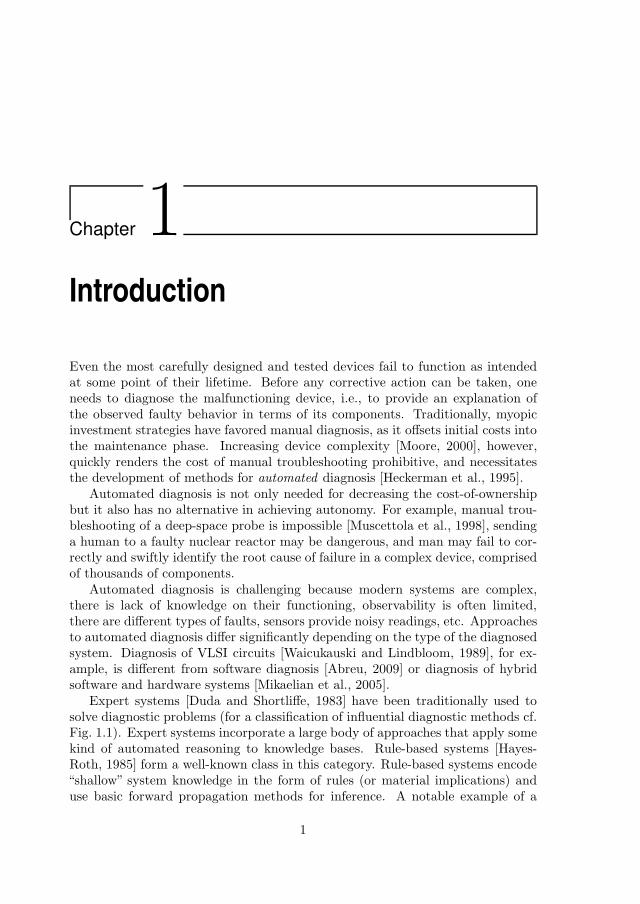
Chapter 1Introduction
Even the most carefully designed and tested devices fail to function as intendedat some point of their lifetime. Before any corrective action can be taken, oneneeds to diagnose the malfunctioning device, i.e., to provide an explanation ofthe observed faulty behavior in terms of its components. Traditionally, myopicinvestment strategies have favored manual diagnosis, as it offsets initial costs intothe maintenance phase. Increasing device complexity [Moore, 2000], however,quickly renders the cost of manual troubleshooting prohibitive, and necessitatesthe development of methods for automated diagnosis [Heckerman et al., 1995].
Automated diagnosis is not only needed for decreasing the cost-of-ownershipbut it also has no alternative in achieving autonomy. For example, manual trou-bleshooting of a deep-space probe is impossible [Muscettola et al., 1998], sendinga human to a faulty nuclear reactor may be dangerous, and man may fail to cor-rectly and swiftly identify the root cause of failure in a complex device, comprisedof thousands of components.
Automated diagnosis is challenging because modern systems are complex,there is lack of knowledge on their functioning, observability is often limited,there are different types of faults, sensors provide noisy readings, etc. Approachesto automated diagnosis differ significantly depending on the type of the diagnosedsystem. Diagnosis of VLSI circuits [Waicukauski and Lindbloom, 1989], for ex-ample, is different from software diagnosis [Abreu, 2009] or diagnosis of hybridsoftware and hardware systems [Mikaelian et al., 2005].
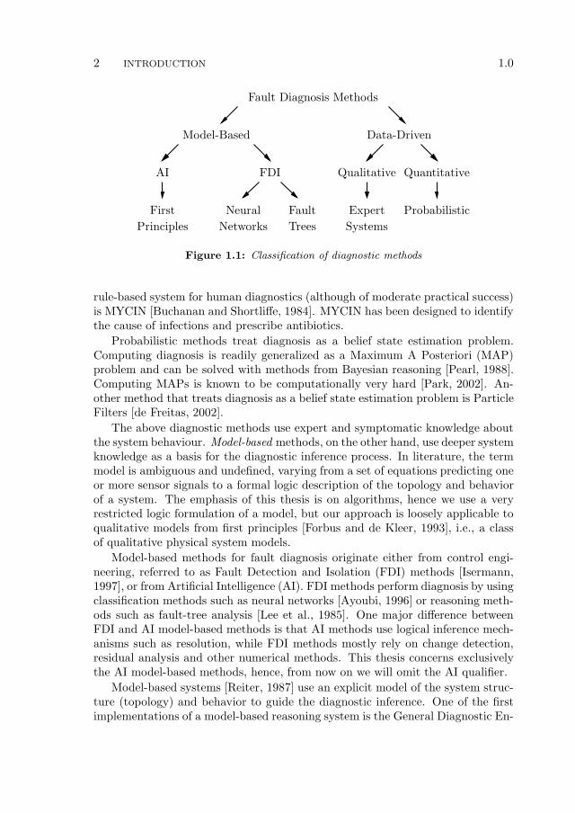
Expert systems [Duda and Shortliffe, 1983] have been traditionally used tosolve diagnostic problems (for a classification of influential diagnostic methods cf.Fig. 1.1). Expert systems incorporate a large body of approaches that apply somekind of automated reasoning to knowledge bases. Rule-based systems [Hayes-Roth, 1985] form a well-known class in this category. Rule-based systems encode“shallow” system knowledge in the form of rules (or material implications) anduse basic forward propagation methods for inference. A notable example of a
1
2 INTRODUCTION 1.0
First
Principles Networks
Neural
Systems
ExpertFault
Trees
FDIAI Quantitative
Probabilistic
Model-Based
Qualitative
Data-Driven
Fault Diagnosis Methods
Figure 1.1: Classification of diagnostic methods
rule-based system for human diagnostics (although of moderate practical success)is MYCIN [Buchanan and Shortliffe, 1984]. MYCIN has been designed to identifythe cause of infections and prescribe antibiotics.
Probabilistic methods treat diagnosis as a belief state estimation problem.Computing diagnosis is readily generalized as a Maximum A Posteriori (MAP)problem and can be solved with methods from Bayesian reasoning [Pearl, 1988].Computing MAPs is known to be computationally very hard [Park, 2002]. An-other method that treats diagnosis as a belief state estimation problem is ParticleFilters [de Freitas, 2002].
The above diagnostic methods use expert and symptomatic knowledge aboutthe system behaviour. Model-based methods, on the other hand, use deeper systemknowledge as a basis for the diagnostic inference process. In literature, the termmodel is ambiguous and undefined, varying from a set of equations predicting oneor more sensor signals to a formal logic description of the topology and behaviorof a system. The emphasis of this thesis is on algorithms, hence we use a veryrestricted logic formulation of a model, but our approach is loosely applicable toqualitative models from first principles [Forbus and de Kleer, 1993], i.e., a classof qualitative physical system models.
Model-based methods for fault diagnosis originate either from control engi-neering, referred to as Fault Detection and Isolation (FDI) methods [Isermann,1997], or from Artificial Intelligence (AI). FDI methods perform diagnosis by usingclassification methods such as neural networks [Ayoubi, 1996] or reasoning meth-ods such as fault-tree analysis [Lee et al., 1985]. One major difference betweenFDI and AI model-based methods is that AI methods use logical inference mech-anisms such as resolution, while FDI methods mostly rely on change detection,residual analysis and other numerical methods. This thesis concerns exclusivelythe AI model-based methods, hence, from now on we will omit the AI qualifier.
Model-based systems [Reiter, 1987] use an explicit model of the system struc-ture (topology) and behavior to guide the diagnostic inference. One of the firstimplementations of a model-based reasoning system is the General Diagnostic En-
1.1 MODEL-BASED DIAGNOSIS 3
gine (GDE) [de Kleer and Williams, 1987]. Model-based systems rely on modelsfrom first principles, i.e., models that represent the basic, real-world, physicalproperties of the diagnosed system.
Model-based diagnostic problems are mostly optimization problems as opposedto decision procedures [Krentel, 1986]. This optimization view naturally mapsmany diagnostic problems into a cost-minimization framework. For example,a diagnostician may be interested in computing the “smallest” explanation of afault (i.e., the minimal or most cost-optimal set of components that have to berepaired), the minimal reconfiguration of a system exposing a given fault, etc.
Many non-linear optimization problems (for example Max-SAT [Hoos andStutzle, 2004]) are hard to solve. Algorithm designers use approximation algo-rithms [Hochbaum, 1997] to find suboptimal solutions of high quality (i.e., solu-tions close to the optimal solution), trading optimality for drastic cost reduction.Approximation algorithms have been successful in providing better cost trade-offs in solving many optimization problems, hence the idea of applying them toautomated diagnosis, which is the focus of this thesis.
1.1 Model-Based Diagnosis
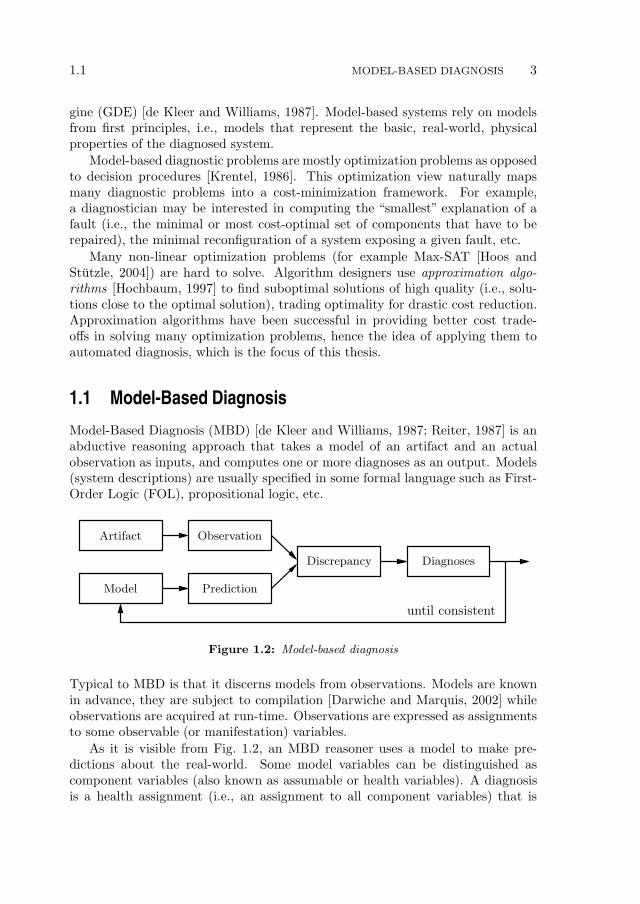
Model-Based Diagnosis (MBD) [de Kleer and Williams, 1987; Reiter, 1987] is anabductive reasoning approach that takes a model of an artifact and an actualobservation as inputs, and computes one or more diagnoses as an output. Models(system descriptions) are usually specified in some formal language such as First-Order Logic (FOL), propositional logic, etc.
Model Prediction
Artifact Observation
Discrepancy Diagnoses
until consistent
Figure 1.2: Model-based diagnosis
Typical to MBD is that it discerns models from observations. Models are knownin advance, they are subject to compilation [Darwiche and Marquis, 2002] whileobservations are acquired at run-time. Observations are expressed as assignmentsto some observable (or manifestation) variables.
As it is visible from Fig. 1.2, an MBD reasoner uses a model to make pre-dictions about the real-world. Some model variables can be distinguished ascomponent variables (also known as assumable or health variables). A diagnosisis a health assignment (i.e., an assignment to all component variables) that is
4 INTRODUCTION 1.1
consistent with a model and an observation. Alternatively, a diagnosis is a set ofcomponents that must be simultaneously faulty to explain an observation. Often,a model cannot predict the faulty behavior of a system because the faulty be-havior is unknown or too complex to describe. Such models are called weak -faultmodels or models with ignorance of abnormal behavior [de Kleer et al., 1992a].Models that capture faulty behavior are called strong-fault models.1 As we willsee in this thesis, model weakness has profound consequences for the diagnosticinference process.
There are many situations in which an MBD reasoner returns multiple diag-nostic candidates: incomplete modeling, sensor-lean systems, weak-fault models,etc. Often the number of diagnoses is exponential in the number of components.This poses a problem for many applications as the residual diagnostic work thathas to be performed by the diagnostician to uniquely isolate the faulty compo-nents becomes prohibitive. The application of lex parsimoniae, however, makessome diagnoses preferred over the others. To first compute the preferred diag-noses, a diagnostic algorithm may impose a (partial) ordering by employing someminimality criterion such as the number of faulty components involved in a diag-nosis. The number of faulty components determines the cardinality of a diagnosisand cardinality-minimality is a common minimality criterion. Another minimalitycriterion is subset-minimality–preferred are diagnoses that do not “contain” otherdiagnoses. In some cases components have a priori probability of failure that canbe obtained, for example, from reliability analysis [Ebeling, 1997]. The applica-tion of diagnosis converts this a priori probability to a posteriori probability (theprobability of failure given the model and the observation).
Applying the cardinality minimality criterion results in cardinality-minimaldiagnoses, i.e., diagnoses that minimize the number of simultaneously faulty com-ponents. The subset-minimality criterion leads to subset-minimal diagnoses. Ifwe consider a diagnosis as a set of faulty components, subset-minimal diagnosesare minimal under set inclusion. Finally, probability-minimal diagnoses minimizethe a posteriori probability of a fault. The a posteriori probability is usually com-puted by updating prior failure probabilities with the help of Bayes’ rule [de Kleerand Williams, 1987].
A minimality criterion alone is often inadequate to optimally reduce the setof diagnoses (the ideal result is one, possibly multiple-fault, diagnosis that is thetrue diagnosis). To further reduce diagnostic uncertainty, a diagnostician canapply MBD multiple times, acquiring additional information at each step. Thisprocess is called sequential diagnosis. One approach to sequential diagnosis is tomeasure unobserved variables in order to decrease the diagnostic uncertainty. Thisprocess is known as probing [de Kleer and Williams, 1987]. In addition to probing,one may actively manipulate a system (or apply tests) to reduce the number of
1Contrary to intuition, strong-fault models are not always preferable over weak-fault ones.MBD knows relatively little research on model “correctness” and from experience, strong-faultmodels are more likely to contain incorrect constraints leading to contradictions or wrong pre-dictions.
1.2 PROBLEM STATEMENT 5
diagnoses. The latter approach for decreasing the diagnostic uncertainty is knownas active testing.
1.2 Problem Statement
Consider a system of n components (n can be thousands) where each componentcan be either healthy or faulty. An algorithm computing diagnosis in such asystem has to consider a search space of size O(2n). There exist sets of restrictionsunder which computing the first subset-minimal diagnosis is in P (for example,weak-fault models allowing polynomial-time consistency checking), but even inthose, computing the first cardinality-minimal diagnosis is NP -hard [Selman andLevesque, 1990]. Computing the second minimal diagnosis is always NP -hard,regardless of the minimality criterion [Bylander et al., 1991]. Sequential MBDis as complex or more complex than the above, combinational MBD, hence allcomplexity problems of combinational MBD are carried over in the sequentialMBD domain.
The overall cost C of automated diagnosis can be expressed as
C = T +W (1.1)
where T is the cost of computing the set of diagnostic candidates (in terms ofCPU time and memory consumption) and W is the residual work (often in termsof manual labor) of finding the actual diagnosis within the list of candidates.
T and W are related. Typically, an exponential increase in T leads to a smalldecrease in W . In computing diagnoses, the decrease in W is according to thelaw of diminishing returns. The reason for that is that computing each separatediagnosis may lead to a combinatorial blowup, while the contribution of a singlediagnosis in deriving the a posteriori fault-state probability distribution function(pdf) of each component is small.
Diagnoses of small cardinality contribute most to decreasing W , given theirrelatively high probability of being the actual fault state. As a result, determin-istic algorithms like CDA∗ [Williams and Ragno, 2007], NGDE [de Kleer, 2009],and RODON [Bunus et al., 2009] generate candidates in order of increasing car-dinality. This approach is slow with high-cardinality faults. For example, in asystem with 1 000 components, if the leading diagnosis is of cardinality 5, thereare approximately 4×10¹² different health assignments containing 4 faults or lessthat may have to be considered first.
Some deterministic algorithms increase their performance by using conflicts(a conflict is a set of components that cannot be simultaneously healthy givena system description and an observation). GDE [de Kleer and Williams, 1987],for example, computes all minimal conflicts prior to computing diagnoses, whileCDA∗ improves the performance of the diagnostic search by learning conflicts ofsmall size. However, the performance problem remains, as minimal conflicts are
6 INTRODUCTION 1.2
dual to minimal diagnoses and hence, computing them is of the same, prohibitivecomputational complexity.
Due to the nature of most MBD problems the return in W diminishes whenincreasing the number and the cardinality of diagnoses. As a result, deterministicalgorithms trade increasingly smaller decreases in W for a large investment in T .A key disadvantage of the majority of deterministic MBD algorithms is that theydo not efficiently exploit the large, continuous solution subspaces2 inherent tomany MBD problems. Extreme examples are the diagnosis spaces in weak-faultmodels where continuity is fundamental, but near-continuous subspaces exist inalmost all diagnostic models. Continuous subspaces also appear in sequentialMBD problems, for example when searching for optimal test vectors.
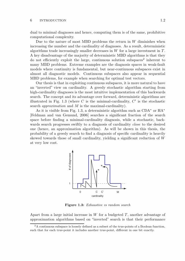
Our thesis is that in exploiting continuous subspaces, it is more natural to havean “inverted” view on cardinality. A greedy stochastic algorithm starting fromhigh-cardinality diagnoses is the most intuitive implementation of this backwardssearch. The concept and its advantage over forward, deterministic algorithms areillustrated in Fig. 1.3 (where C is the minimal-cardinality, C′ is the stochasticsearch approximation and M is the maximal-cardinality).
As it is visible from Fig. 1.3, a deterministic algorithm such as CDA∗ or HA∗
[Feldman and van Gemund, 2006] searches a significant fraction of the searchspace before finding a minimal-cardinality diagnosis, while a stochastic, back-wards search progresses swiftly to a diagnosis of cardinality close to the desiredone (hence, an approximation algorithm). As will be shown in this thesis, theprobability of a greedy search to find a diagnosis of specific cardinality is heavilyskewed towards those of small cardinality, yielding a significant reduction of Wat very low cost.
*
*
cardinality
# o
f d
iag
no
se
s
C C’0 M
1
Figure 1.3: Exhaustive vs random search
Apart from a large initial increase in W for a budgeted T , another advantage ofapproximation algorithms based on “inverted” search is that their performance
2A continuous subspace is loosely defined as a subset of the true-points of a Boolean function,such that for each true-point it includes another true-point, different in one bit exactly.
1.3 CONTRIBUTION 7
degrades more smoothly than the performance of deterministic algorithms, i.e.,approximation algorithms compute results (although sub-optimal) even in thecases in which a deterministic MBD algorithm would run out of computationalresources. That is, approximation algorithms show strong anytime behavior, andwill return results after any non-trivial inference time.
Given the potential of our approximation approach to MBD, the main researchquestion addressed in this thesis is formulated as follows:
What are the cost/performance trade-offs of using approximation al-gorithms for MBD?
In addition to the main research issue above, this thesis also addresses a numberof peripheral questions:
• What are the cost/performance trade-offs of using a greedy approximationalgorithm? Can we analytically or programmatically model the performanceof the approximation algorithms and is it possible to establish bounds onthe optimality of the approximation algorithms by using these models?
• Often MBD algorithms consider multiple observations (tests) to reduce thediagnostic ambiguity. Can a greedy approximation algorithm be used tocompute a sequence of control settings that reduces near-optimally the num-ber of diagnoses?
• An important performance characteristic of diagnostic algorithms is thetime to compute a high-cardinality solution. However, observations lead-ing to such high-cardinality solutions are extremely hard to determine. Cana greedy approximation algorithm be used to compute observations thatmaximize the cardinality of the minimal-cardinality diagnoses?
• As mentioned earlier, a key premise to our approximation approach is searchspace continuity. Until now, it was suspected that continuity exists in weak-fault models only. We have noticed that parts of strong-fault models exposetopologically-dependent continuous properties. Which specific strong-faultmodel/observation properties affect the performance of greedy approxima-tion algorithms?
1.3 Contribution
To our knowledge, we are the first to apply approximation algorithms to MBD.Our contributions are described in the following two sections.
1.3.1 Theory
1. We propose a greedy approximation algorithm, called Safari (StochAsticFault diagnosis AlgoRIthm), to solve the fundamental MBD problem of com-puting minimal diagnoses. We model the progress of Safari and establish
8 INTRODUCTION 1.3
bounds on its performance. We consider the distribution of the cardinali-ties of the diagnoses computed by Safari and establish favorable propertiesof Safari in terms of this distribution. We compare the performance andoptimality of Safari to, amongst others, that of a family of MBD algo-rithms based on stochastic Max-SAT. We empirically demonstrate, usingthe 74XXX and ISCAS85 suites of benchmark combinatorial circuits, thatSafari achieves several orders-of-magnitude speedup over both determinis-tic algorithms and algorithms based on stochastic Max-SAT.
2. We combine approaches from sequential diagnosis [Shakeri, 1996], passivemonitoring [Pietersma and van Gemund, 2006], probing [de Kleer and Wil-liams, 1987], and Automated Test Pattern Generation (ATPG), into anMBD framework called Fractal (FRamework for ACtive Testing ALgo-rithms). We propose an algorithm, called FractalG, that approximatesthe computationally hard problem of computing optimal control assignments(as defined in Fractal). FractalG offers a low-cost, greedy, stochasticapproach that maintains exponential decay of the number of cardinality-minimal diagnoses computed by Safari. We compare the performance ofFractalG to FractalA (ATPG-based sequential diagnosis) and Frac-
talP (probing). FractalG overcomes limitations of FractalA and offersa trade-off in computational complexity versus optimality in reducing thediagnostic uncertainty. We use FractalP to show lower bound on the decayof Safari diagnoses, achievable for a model extended with unlimited con-trol circuitry. We present extensive empirical data on Fractal experimentswith models of the 74XXX/ISCAS85 combinational circuits.
3. We define the so called Max-Fault Min-Cardinality (MFMC) problem offinding an observation that leads to a minimum-cardinality diagnosis thathas the highest possible number of faults given a system description, and useMFMC observation vectors for benchmarking the performance of combina-tional MBD algorithms. We present a near-optimal, stochastic algorithm,called Miranda (Max-fault mIn-caRdinAlity observatioN Deduction Algo-rithm), that computes observations leading to diagnoses of large cardinality.Experiments show that Miranda delivers optimal results on the 74XXX cir-cuits, as well as good MFMC cardinality estimates on the larger ISCAS85circuits.
1.3.2 Application
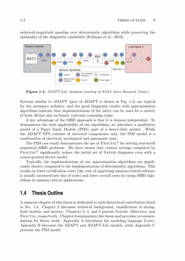
The MBD approximation algorithms discussed in this thesis are validated in termsof their practical significance. We have applied them, amongst others, to a modelof the Electrical Power System (EPS) testbed in the ADAPT lab at NASA AmesResearch Center [Poll et al., 2007]. ADAPT EPS has been a part of the FirstInternational Diagnostic Competition (DXC’09) where Safari has shown several
1.4 THESIS OUTLINE 9
orders-of-magnitude speedup over deterministic algorithms while preserving theoptimality of the diagnostic candidates [Feldman et al., 2010].
E265
ST
265
CB236 CB266
Battery Cabinet
EY260
ESH
260AE261
IT261
E267
IT267
Load Bank 2
120V AC >>
ISH
262
CB262
ISH
266
BAT2
TE
228
E235 E240
EY244IT240
ESH
244A
TE
229
ISH
236
E242 XT267EY275
ESH
275
ST
516FAN416
INV
2
ESH
ISHE
IT
TE
XT
Voltage
Relay Position
Feedback
Circuit Breaker
Feedback
Current
Temperature
Phase Angle
Sensor Symbols
Figure 1.4: ADAPT-Lite (diagram courtesy of NASA Ames Research Center)
Systems similar to ADAPT (part of ADAPT is shown in Fig. 1.4) are typicalfor the aerospace industry, and the good diagnostic results with approximationalgorithms indicate that implementations of the latter can be used for a varietyof both off-line and on-board, real-time reasoning tasks.
A key advantage of the MBD approach is that it is domain independent. Todemonstrate the wide applicability of our algorithms, we introduce a qualitativemodel of a Paper Input Module (PIM), part of a heavy-duty printer. Whilethe ADAPT EPS consists of electrical components only, the PIM model is acombination of electrical, mechanical and pneumatic ones.
The PIM case study demonstrates the use of FractalG for solving real-worldsequential MBD problems. We have shown that control settings computed byFractalG significantly reduce the initial set of Safari diagnoses even with acoarse-grained device model.
Typically, the implementations of our approximation algorithms are signifi-cantly shorter compared to the implementations of deterministic algorithms. Thisresults in lower certification costs (the cost of approving mission-critical softwareis usually measured per line of code) and lower overall costs for using MBD algo-rithms in mission critical applications.
1.4 Thesis Outline
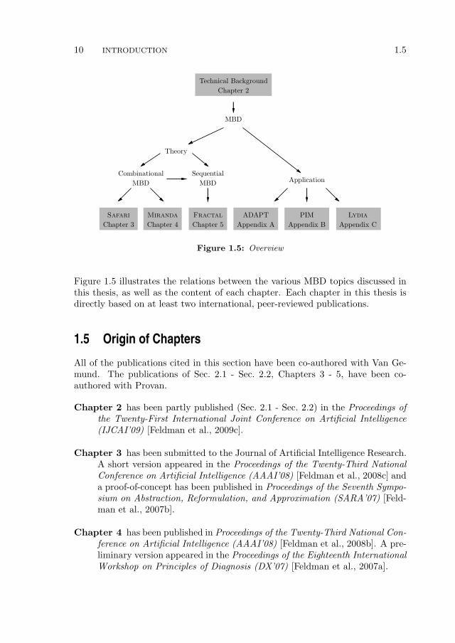
A separate chapter of this thesis is dedicated to each theoretical contribution listedin Sec. 1.3. Chapter 2 discusses technical background, classification of strong-fault models, and metrics. Chapters 3, 4, and 5 present Safari, Miranda, andFractal, respectively. Chapter 6 summarizes this thesis and provides recommen-dations for future work. Appendix A introduces the modeling language Lydia.Appendix B discusses the ADAPT and ADAPT-Lite models, while Appendix Cpresents the PIM model.
10 INTRODUCTION 1.5
PIM
Appendix B Appendix C
LydiaADAPT
Appendix A
Application
Chapter 2
Technical Background
MBD
Fractal
Chapter 5
MBD
Combinational
Safari
Chapter 3 Chapter 4
Miranda
MBD
Sequential
Theory
Figure 1.5: Overview
Figure 1.5 illustrates the relations between the various MBD topics discussed inthis thesis, as well as the content of each chapter. Each chapter in this thesis isdirectly based on at least two international, peer-reviewed publications.
1.5 Origin of Chapters
All of the publications cited in this section have been co-authored with Van Ge-mund. The publications of Sec. 2.1 - Sec. 2.2, Chapters 3 - 5, have been co-authored with Provan.
Chapter 2 has been partly published (Sec. 2.1 - Sec. 2.2) in the Proceedings ofthe Twenty-First International Joint Conference on Artificial Intelligence(IJCAI’09) [Feldman et al., 2009c].
Chapter 3 has been submitted to the Journal of Artificial Intelligence Research.A short version appeared in the Proceedings of the Twenty-Third NationalConference on Artificial Intelligence (AAAI’08) [Feldman et al., 2008c] anda proof-of-concept has been published in Proceedings of the Seventh Sympo-sium on Abstraction, Reformulation, and Approximation (SARA’07) [Feld-man et al., 2007b].
Chapter 4 has been published in Proceedings of the Twenty-Third National Con-ference on Artificial Intelligence (AAAI’08) [Feldman et al., 2008b]. A pre-liminary version appeared in the Proceedings of the Eighteenth InternationalWorkshop on Principles of Diagnosis (DX’07) [Feldman et al., 2007a].

1.5 ORIGIN OF CHAPTERS 11
Chapter 5 has been submitted to the Journal of Artificial Intelligence Research.A preliminary version has been published in the Proceedings of the Twenty-First International Joint Conference on Artificial Intelligence (IJCAI’09)[Feldman et al., 2009b] and a proof-of-concept appeared in the Proceedings ofthe First International Conference on Prognostics and Health Management(PHM’08) [Feldman et al., 2008a].
Appendix A originally appeared as a Technical Report [Feldman and van Ge-mund, 2007b].
Appendix B is submitted to the International Journal of Prognostics and HealthManagement.
Appendix C originally appeared as a Technical Report [Feldman and van Ge-mund, 2009].

12 INTRODUCTION 1.5

Chapter 2Model-Based Diagnosis
Model-based diagnosis, as formulated in terms of logic [Reiter, 1987], focuses ondetermining whether an assignment of health/failure states to a set of behavioralmode variables is consistent with a system description and an observation (e.g., ofsensor values). Hence, the diagnostic process consists of taking an observation (oran observation vector), and then inferring the failure-mode assignment (diagnosis)consistent with that observation(s).
2.1 Concepts and Definitions
Our discussion continues by formalizing some MBD notions. This thesis uses thetraditional diagnostic definitions [de Kleer and Williams, 1987], except that weuse propositional logic terms (conjunctions of literals) instead of sets of failingcomponents.
Central to MBD, a model of an artifact is represented as a Well-Formed Propo-sitional Formula (Wff) over some set of variables. We discern subsets of thesevariables as assumable and observable.1
Definition 1 (Diagnostic System). A diagnostic system DS is defined as thetriple DS = 〈SD,COMPS,OBS〉, where SD is a propositional theory over a set ofvariables V , COMPS ⊆ V is the set of assumables, and OBS ⊆ V is the set ofobservables.
Throughout this thesis we will assume that OBS ∩COMPS = ∅ and SD 6|=⊥.Let COMPS = h1, h2, · · · , hn. This mnemonics corresponds to the conven-
tion that a positive sign of a “health” variable (h1, h2, · · · , hn) denotes a nominal
1In the MBD literature the assumable variables are also referred to as “component”, “failure-mode”, or “health” variables. Observable variables are also called “measurable”, or “control”variables.
13
14 MODEL-BASED DIAGNOSIS 2.1
(healthy) component state. Faulty components are denoted as ¬h1,¬h2, · · · ,¬hn.Other authors use “ab” for abnormal or “ok” for healthy.
Not all propositional theories used as system descriptions are of interest toMBD. Diagnostic systems can be characterized by a restricted set of models, therestriction making the problem of computing diagnosis amenable to algorithmslike the ones presented in this thesis. We consider two main classes of models.
Definition 2 (Weak-Fault Model). A diagnostic system DS = 〈SD, COMPS,OBS〉 belongs to the class WFM iff SD is equivalent to (h1 ⇒ F1) ∧ (h2 ⇒F2) ∧ · · · ∧ (hn ⇒ Fn) such that for 1 ≤ i ≤ n, hi ⊆ COMPS, Fi ∈Wff , andCOMPS∩V ′ = ∅, where V ′ is the set of all variables appearing in F1, F2, · · · , Fn.
Weak-fault models are sometimes referred to as models with ignorance of abnor-mal behavior [de Kleer et al., 1992a], or implicit fault systems. Alternatively, amodel may specify faulty behavior for its components. In the following defini-tion, with the aim of simplifying the formalism throughout this thesis, we adopt aslightly restrictive representation of faults, allowing only a single fault mode perassumable variable. This can be easily generalized by introducing multi-valuedlogic or suitable encodings [Feldman et al., 2006; Hoos, 1999].
Definition 3 (Strong-Fault Model). A diagnostic system DS = 〈SD, COMPS,OBS〉 belongs to the class SFM iff SD is equivalent to (h1 ⇒ F1,1) ∧ (¬h1 ⇒F1,2) ∧ · · · ∧ (hn ⇒ Fn,1) ∧ (¬hn ⇒ Fn,2) such that 1 ≤ i, j ≤ n, k ∈ 1, 2,hi ⊆ COMPS, Fj,k ∈Wff , and none of hi appears in Fj,k.
Membership testing for the WFM and SFM classes can be performed efficientlyin many cases, for example, when a model is represented explicitly as in Def. 2 orDef. 3.
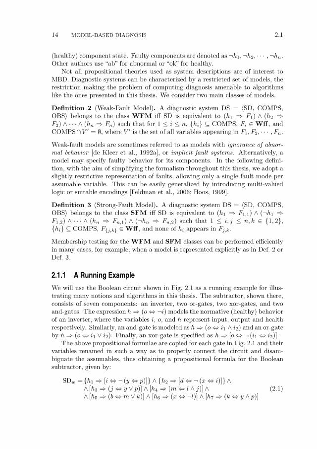
2.1.1 A Running Example
We will use the Boolean circuit shown in Fig. 2.1 as a running example for illus-trating many notions and algorithms in this thesis. The subtractor, shown there,consists of seven components: an inverter, two or-gates, two xor-gates, and twoand-gates. The expression h⇒ (o⇔ ¬i) models the normative (healthy) behaviorof an inverter, where the variables i, o, and h represent input, output and healthrespectively. Similarly, an and-gate is modeled as h⇒ (o⇔ i1 ∧ i2) and an or-gateby h⇒ (o⇔ i1 ∨ i2). Finally, an xor-gate is specified as h⇒ [o⇔ ¬ (i1 ⇔ i2)].
The above propositional formulae are copied for each gate in Fig. 2.1 and theirvariables renamed in such a way as to properly connect the circuit and disam-biguate the assumables, thus obtaining a propositional formula for the Booleansubtractor, given by:
SDw = h1 ⇒ [i⇔ ¬ (y ⇔ p)] ∧ h2 ⇒ [d⇔ ¬ (x⇔ i)]∧∧ [h3 ⇒ (j ⇔ y ∨ p)] ∧ [h4 ⇒ (m⇔ l ∧ j)]∧∧ [h5 ⇒ (b⇔ m ∨ k)] ∧ [h6 ⇒ (x⇔ ¬l)] ∧ [h7 ⇒ (k ⇔ y ∧ p)]
(2.1)

2.1 CONCEPTS AND DEFINITIONS 15
h2d
h6yp h1
h3h4j
i
h5
h7
x
m
k
b
l
Figure 2.1: A subtractor circuit
A strong-fault model for the Boolean circuit shown in Fig. 2.1 is constructed byassigning fault-modes to the different gate types. We will assume that, whenmalfunctioning, the output of an xor-gate has the value of one of its inputs, anor-gate can be stuck-at-one, an and-gate can be stuck-at-zero, and an inverterbehaves like a buffer. This gives us the following strong-fault model formula forthe Boolean subtractor circuit:
SDs = SDw ∧ [¬h1 ⇒ (i⇔ y)] ∧ [¬h2 ⇒ (d⇔ x)] ∧ (¬h3 ⇒ j)∧∧ (¬h4 ⇒ ¬m) ∧ (¬h5 ⇒ b) ∧ [¬h6 ⇒ (x⇔ l)] ∧ (¬h7 ⇒ ¬k) (2.2)
For both models (SDs and SDw), the set of assumable variables is COMPS =h1, h2, · · · , h7 and the set of observable variables is OBS = x, y, p, d, b.
2.1.2 Diagnosis and Minimal Diagnosis
The traditional query in MBD computes terms of assumable variables which areexplanations for the system description and an observation.
Definition 4 (Health Assignment). Given a system DS = 〈SD, COMPS, OBS〉,an assignment ω to all variables in COMPS is defined as a health assignment.
A health assignment ω is represented as a conjunction of propositional literals.In some cases it is convenient to use the set of negative or positive literals in ω.These two sets are denoted as Lit−(ω) and Lit+(ω), respectively.
In our example, the “all nominal” assignment is ω1 = h1 ∧ h2 ∧ · · · ∧ h7. Thehealth assignment ω2 = h1 ∧ h2 ∧ h3 ∧ ¬h4 ∧ h5 ∧ h6 ∧ ¬h7 means that the twoand-gates from Fig. 2.1 are malfunctioning.
What follows is a formal definition of consistency-based diagnosis.
Definition 5 (Diagnosis). Given a diagnostic system DS = 〈SD,COMPS,OBS〉,an observation α over some variables in OBS, and a health assignment ω, ω is adiagnosis iff SD ∧ α ∧ ω 6|=⊥.
16 MODEL-BASED DIAGNOSIS 2.1
Traditionally, other authors [de Kleer and Williams, 1987] arrive at minimal di-agnosis by computing a minimal hitting set of the minimal conflicts (broadly,minimal health assignments incompatible with the system description and theobservation), while this thesis makes no use of conflicts, hence the equivalent,direct definition above.
There is a total of 96 possible diagnoses given SDw and an observation α1 =x ∧ y ∧ p ∧ b ∧ ¬d. Example diagnoses are ω3 = ¬h1 ∧ h2 ∧ · · · ∧ h7 and ω4 =h1 ∧ ¬h2 ∧ h3 ∧ · · · ∧ h7. Trivially, given a weak-fault model, the “all faulty”health assignment (in our example ωa = ¬h1 ∧ · · · ∧ ¬h7) is a diagnosis for anyinstantiation of the observable variables in OBS (cf. Def. 2).
In the MBD literature, a range of types of “preferred” diagnosis has beenproposed. This turns the MBD problem into an optimization problem. In thefollowing definition we consider the common subset-ordering.
Definition 6 (Minimal Diagnosis). A diagnosis ω⊆ is defined as minimal, if nodiagnosis ω⊆ exists such that Lit−(ω⊆) ⊂ Lit−(ω⊆).
Consider the weak-fault model SDw of the circuit shown in Fig. 2.1 and an obser-vation α2 = ¬x∧y∧p∧¬b∧d. In this example, two of the minimal diagnoses areω⊆
5 = ¬h1 ∧h2 ∧h3 ∧h4∧¬h5 ∧h6 ∧h7 and ω⊆6 = ¬h1 ∧h2 ∧ · · ·∧h5 ∧¬h6 ∧¬h7.
The diagnosis ω7 = ¬h1 ∧ ¬h2 ∧ h3 ∧ h4 ∧ ¬h5 ∧ h6 ∧ h7 is non-minimal as thenegative literals in ω⊆
5 form a subset of the negative literals in ω7.
Note that the set of all minimal diagnoses characterizes all diagnoses fora weak-fault model, but that does not hold in general for strong-fault models[de Kleer et al., 1992a]. In the latter case, faulty components may “exonerate”each other, resulting in a health assignment containing a proper superset of thenegative literals of another diagnosis not to be a diagnosis. In our example, givenSDs and α3 = ¬x∧¬y∧¬p∧b∧¬d, it follows that ω⊆
8 = h1∧h2∧¬h3∧h4∧· · ·∧h7
is a diagnosis, but ω9 = h1 ∧ h2 ∧ ¬h3 ∧ ¬h4 ∧ · · · ∧ h7 is not a diagnosis, despitethe fact that the set of negative literals in ω9 (¬h3,¬h4) forms a superset of
the set of negative literals in ω⊆8 (¬h3).
Definition 7 (Number of Minimal Diagnoses). Let the set Ω⊆(SD ∧ α) containall minimal diagnoses of a system description SD and an observation α. Thenumber of minimal diagnoses, denoted as |Ω⊆(SD ∧ α)|, is defined as the size ofΩ⊆(SD ∧ α).
Continuing our running example, |Ω⊆(SDw ∧ α2)| = 8 and |Ω⊆(SDs ∧ α3)| = 2.The number of non-minimal diagnoses of SDw ∧ α2 is 61.
Definition 8 (Cardinality of a Diagnosis). The cardinality of a diagnosis, denotedas |ω|, is defined as the number of negative literals in ω.
Diagnosis cardinality gives us another partial ordering: a diagnosis is defined asminimal cardinality iff it minimizes the number of negative literals.
2.2 DIAGNOSTIC MODEL TAXONOMY 17
Definition 9 (Minimal-Cardinality Diagnosis). A diagnosis ω≤ is defined asminimal-cardinality if no diagnosis ω≤ exists such that |ω≤| < |ω≤|.The cardinality of a minimal-cardinality diagnosis computed from a system de-scription SD and an observation α is denoted as MinCard(SD ∧ α). For ourexample model SDw and an observation α4 = x ∧ y ∧ p ∧ ¬b ∧ ¬d , it follows thatMinCard(SDw ∧ α4) = 2. Note that in this case all minimal diagnoses are alsominimal-cardinality diagnoses.
A minimal cardinality diagnosis is a minimal diagnosis, but the opposite doesnot hold. There are minimal diagnoses that are not minimal-cardinality diagnoses.Consider the example SDw and α2 given earlier in this section, and the tworesulting minimal diagnoses ω⊆
5 and ω⊆6 . From these two, only ω⊆
5 is a minimal-cardinality diagnosis.
Definition 10 (Number of Minimal-Cardinality Diagnoses). Let the set Ω≤(SD∧α) contain all minimal-cardinality diagnoses of a system description SD and anobservationα. The number of minimal-cardinality diagnoses, denoted as |Ω≤(SD∧α)|, is defined as the cardinality of Ω≤(SD ∧ α).
Computing the number of minimal-cardinality diagnoses for the running exampleresults in |Ω≤(SDw ∧ α2)| = 2, |Ω≤(SDs ∧ α3)| = 2, and |Ω≤(SDw ∧ α4)| = 4.
2.2 Diagnostic Model Taxonomy
Within MBD, two broad classes of model types have been specified: weak-faultmodels WFM [de Kleer et al., 1992a] and strong-fault models SFM [Struss andDressler, 1989]. Traditionally, WFM has been considered to be computationallysimple, and SFM computationally hard. Weak-fault models describe a systemonly in terms of its normal (non-faulty) behaviour, whereas strong-fault modelsinclude a definition of some aspects of abnormal behaviour. Strong-fault modelscan avoid violating physical rules (cf. [Struss and Dressler, 1989]), but at the costof increased complexity: moving from a binary-valued model with n components(which is adequate for weak-fault models) to one with m+1 possible faulty valuesincreases the maximum number of failure candidates from 2n to (m+ 1)n.
In terms of worst-case complexity, finding the first minimal diagnosis for aHorn model in WFM can be done in polynomial time, but finding the nextminimal diagnosis is NP-complete [Friedrich et al., 1990]. In contrast, inferencein strong-fault models entails computing kernel diagnoses [de Kleer et al., 1992a],which is a ΣP
2 -hard task and is known to be computationally intensive in practice;for example, kernel diagnoses are given by the prime implicants of the minimalconflicts [de Kleer et al., 1992a]. Further, the average case complexity of reasoningin WFM versus SFM increases from poly-time in n (WFM) to exponential inn (SFM) [de Kleer et al., 1992a].
We show that, by closer examination of SFM, there is a spectrum of modeltypes, and, possibly, corresponding inference complexities. We identify two main
18 MODEL-BASED DIAGNOSIS 2.2
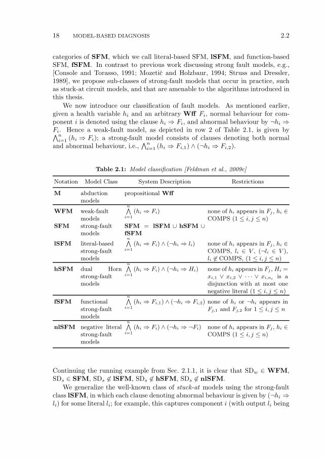
categories of SFM, which we call literal-based SFM, lSFM, and function-basedSFM, fSFM. In contrast to previous work discussing strong fault models, e.g.,[Console and Torasso, 1991; Mozetic and Holzbaur, 1994; Struss and Dressler,1989], we propose sub-classes of strong-fault models that occur in practice, suchas stuck-at circuit models, and that are amenable to the algorithms introduced inthis thesis.
We now introduce our classification of fault models. As mentioned earlier,given a health variable hi and an arbitrary Wff Fi, normal behaviour for com-ponent i is denoted using the clause hi ⇒ Fi, and abnormal behaviour by ¬hi ⇒Fi. Hence a weak-fault model, as depicted in row 2 of Table 2.1, is given by∧n
i=1 (hi ⇒ Fi); a strong-fault model consists of clauses denoting both normaland abnormal behaviour, i.e.,
∧ni=1 (hi ⇒ Fi,1) ∧ (¬hi ⇒ Fi,2).
Table 2.1: Model classification [Feldman et al., 2009c]
Notation Model Class System Description Restrictions
M abductionmodels
propositional Wff
WFM weak-faultmodels
n∧i=1
(hi ⇒ Fi) none of hi appears in Fj , hi ∈COMPS (1 ≤ i, j ≤ n)
SFM strong-faultmodels
SFM = lSFM ∪ hSFM ∪fSFM
lSFM literal-basedstrong-faultmodels
n∧i=1
(hi ⇒ Fi) ∧ (¬hi ⇒ li) none of hi appears in Fj , hi ∈COMPS, li ∈ V , (¬li ∈ V ),li 6∈ COMPS, (1 ≤ i, j ≤ n)
hSFM dual Hornstrong-faultmodels
n∧i=1
(hi ⇒ Fi) ∧ (¬hi ⇒ Hi) none of hi appears in Fj , Hi =xi,1 ∨ xi,2 ∨ · · · ∨ xi,ni
is adisjunction with at most onenegative literal (1 ≤ i, j ≤ n)
fSFM functionalstrong-faultmodels
n∧i=1
(hi ⇒ Fi,1) ∧ (¬hi ⇒ Fi,2) none of hi or ¬hi appears inFj,1 and Fj,2 for 1 ≤ i, j ≤ n
nlSFM negative literalstrong-faultmodels
n∧i=1
(hi ⇒ Fi) ∧ (¬hi ⇒ ¬Fi) none of hi appears in Fj , hi ∈COMPS (1 ≤ i, j ≤ n)
Continuing the running example from Sec. 2.1.1, it is clear that SDw ∈ WFM,SDs ∈ SFM, SDs 6∈ lSFM, SDs 6∈ hSFM, SDs 6∈ nlSFM.
We generalize the well-known class of stuck-at models using the strong-faultclass lSFM, in which each clause denoting abnormal behaviour is given by (¬hi ⇒li) for some literal li; for example, this captures component i (with output li being
2.3 CONVERTING PROPOSITIONAL FORMULAE TO CLAUSAL FORM 19
stuck-at-0) as given by [(hi = stuck-at-0) ⇒ (li = 0)].The class hSFM of dual Horn strong-fault models has the consequent Wff Fi
restricted to dual Horn clauses (clauses with at most one negative literal). Theclass fSFM of functional strong-fault models allows the consequent Wff Fi to takeon any form. Finally, the class nlSFM of negative-literal strong-fault models hasthe consequent Wff Fi restricted to defining the negation of the normal behaviourof component i given hi.
In the above classification we do not address the problem of recognizing if amodel SD belongs to a specific class. This problem is expected to be hard in thegeneral case (arbitrary Wff and class). In some specific cases (e.g., an explicitmodel representation from Table 2.1), recognition can be done efficiently.
Determining the model class has consequences for the choice of MBD reasoningalgorithm and for preprocessing the model. Models belonging to lSFM, hSFM,and nlSFM can be relaxed by “stripping” the “stuck-at” constraints and solvedwith a diagnostic solver optimized for WFM. The strong-part of the model canbe solved subsequently, and the set of diagnoses circumscribed [Feldman et al.,2009c].
2.3 Converting Propositional Formulae to Clausal Form
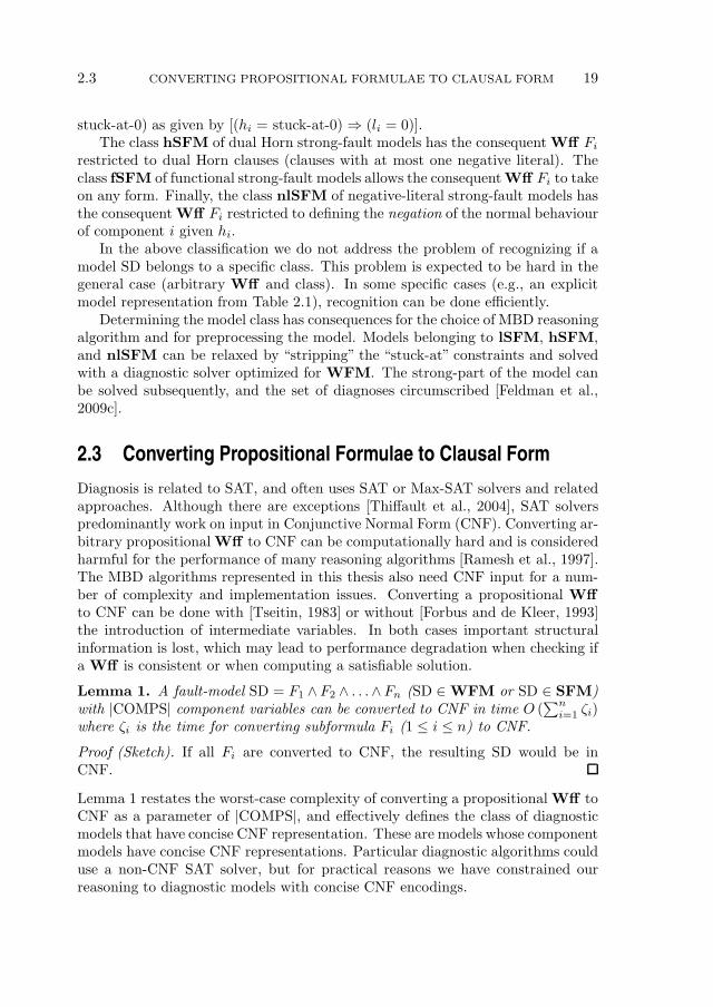
Diagnosis is related to SAT, and often uses SAT or Max-SAT solvers and relatedapproaches. Although there are exceptions [Thiffault et al., 2004], SAT solverspredominantly work on input in Conjunctive Normal Form (CNF). Converting ar-bitrary propositional Wff to CNF can be computationally hard and is consideredharmful for the performance of many reasoning algorithms [Ramesh et al., 1997].The MBD algorithms represented in this thesis also need CNF input for a num-ber of complexity and implementation issues. Converting a propositional Wff
to CNF can be done with [Tseitin, 1983] or without [Forbus and de Kleer, 1993]the introduction of intermediate variables. In both cases important structuralinformation is lost, which may lead to performance degradation when checking ifa Wff is consistent or when computing a satisfiable solution.
Lemma 1. A fault-model SD = F1 ∧F2 ∧ . . .∧Fn (SD ∈WFM or SD ∈ SFM)with |COMPS| component variables can be converted to CNF in time O (
∑ni=1 ζi)
where ζi is the time for converting subformula Fi (1 ≤ i ≤ n) to CNF.
Proof (Sketch). If all Fi are converted to CNF, the resulting SD would be inCNF.
Lemma 1 restates the worst-case complexity of converting a propositional Wff toCNF as a parameter of |COMPS|, and effectively defines the class of diagnosticmodels that have concise CNF representation. These are models whose componentmodels have concise CNF representations. Particular diagnostic algorithms coulduse a non-CNF SAT solver, but for practical reasons we have constrained ourreasoning to diagnostic models with concise CNF encodings.
20 MODEL-BASED DIAGNOSIS 2.4
Consider, for example, the formula (x1 ∧ y1) ∨ (x2 ∧ y2) ∨ · · · ∨ (xn ∧ yn),which is in Disjunctive Normal Form2 (DNF) and, converted to CNF, has 2n
clauses. Although similar examples of propositional Wff having exponentiallymany clauses in their CNF representations are easy to find, they are artificial andare rarely encountered in MBD (cf. Manolios and Vroon [2007] for benchmarkresults on Boolean circuit Wff to CNF conversion). Furthermore, the Booleancircuits with which we have tested the performance of our algorithms, do not showexponential blow-up when converted to CNF.
2.4 Benchmarks
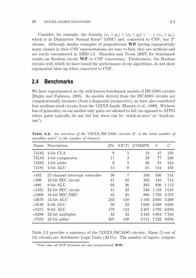
We have experimented on the well-known benchmark models of ISCAS85 circuits[Brglez and Fujiwara, 1985]. As models derived from the ISCAS85 circuits arecomputationally intensive (from a diagnostic perspective), we have also consideredfour medium-sized circuits from the 74XXX family [Hansen et al., 1999]. Withoutloss of generality, in our models only gates are allowed to fail (as opposed to ATPGwhere gates typically do not fail but wires can be “stuck-at-zero” or “stuck-at-one”).
Table 2.2: An overview of the 74XXX/ISCAS85 circuits (V is the total number ofvariables and C is the number of clauses)
Name Description |IN| |OUT| |COMPS| V C
74182 4-bit CLA 9 5 19 47 15074L85 4-bit comparator 11 3 33 77 23674283 4-bit adder 9 5 36 81 24474181 4-bit ALU 14 8 65 144 456
c432 27-channel interrupt controller 36 7 160 356 514c499 32-bit SEC circuit 41 32 202 445 714c880 8-bit ALU 60 26 383 826 1 112c1355 32-bit SEC circuit 41 32 546 1 133 1 610c1908 16-bit SEC/DEC 33 25 880 1 793 2 378c2670 12-bit ALU 233 140 1 193 2 695 3 269c3540 8-bit ALU 50 22 1 669 3 388 4 608c5315 9-bit ALU 178 123 2 307 4 792 6 693c6288 32-bit multiplier 32 32 2 416 4 864 7 216c7552 32-bit adder 207 108 3 512 7 232 9 656
Table 2.2 provides a summary of the 74XXX/ISCAS85 circuits. Many (5 out of14) circuits are Arithmetic Logic Units (ALUs). The number of inputs, outputs
2Note that all DNF formulae are also propositional Wffs.
2.5 DIAGNOSTIC METRICS 21
and components are given in the third, fourth, and fifth column of Table 2.2,respectively. The sixth and seventh columns show the number of variables andclauses, respectively, in the CNF representation of the circuits.
2.5 Diagnostic Metrics
In this section we assume that each diagnostic experiment (a diagnostic scenario)defines a fault injection ω⋆ of minimal-cardinality and an associated observation α.Note that computing 〈α, ω⋆〉 pairs such that |ω⋆| > 1 is not trivial (this problemis addressed in Chapter 4).
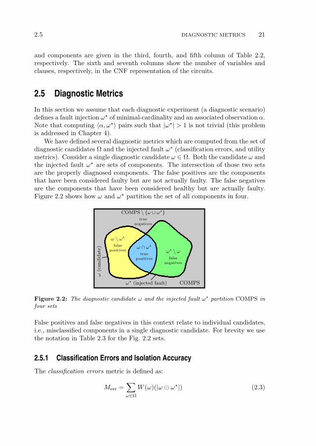
We have defined several diagnostic metrics which are computed from the set ofdiagnostic candidates Ω and the injected fault ω∗ (classification errors, and utilitymetrics). Consider a single diagnostic candidate ω ∈ Ω. Both the candidate ω andthe injected fault ω⋆ are sets of components. The intersection of those two setsare the properly diagnosed components. The false positives are the componentsthat have been considered faulty but are not actually faulty. The false negativesare the components that have been considered healthy but are actually faulty.Figure 2.2 shows how ω and ω⋆ partition the set of all components in four.
positives
ω ∩ ω⋆
true
negatives
COMPS \ ω ∪ ω⋆
true
COMPSω⋆ (injected fault)
ω(c
andid
ate
)
ω⋆ \ ω
falsenegatives
ω \ ω⋆
falsepositives
Figure 2.2: The diagnostic candidate ω and the injected fault ω⋆ partition COMPS infour sets
False positives and false negatives in this context relate to individual candidates,i.e., misclassified components in a single diagnostic candidate. For brevity we usethe notation in Table 2.3 for the Fig. 2.2 sets.
2.5.1 Classification Errors and Isolation Accuracy
The classification errors metric is defined as:
Merr =∑
ω∈Ω
W (ω)(|ω ⊖ ω⋆|) (2.3)
22 MODEL-BASED DIAGNOSIS 2.5
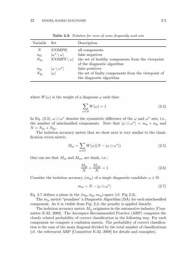
Table 2.3: Notation for sizes of some frequently used sets
Variable Set Description
N |COMPS| all componentsnfn |ω⋆ \ ω| false negativesNfn |COMPS \ ω| the set of healthy components from the viewpoint
of the diagnostic algorithmnfp |ω \ ω⋆| false positivesNfp |ω| the set of faulty components from the viewpoint of
the diagnostic algorithm
where W (ω) is the weight of a diagnosis ω such that:
∑
ω∈Ω
W (ω) = 1 (2.4)
In Eq. (2.3), ω ⊖ ω⋆ denotes the symmetric difference of the ω and ω⋆ sets, i.e.,the number of misclassified components. Note that |ω ⊖ ω⋆| = nfn + nfp andN = Nfn +Nfp.
The isolation accuracy metric that we show next is very similar to the classi-fication errors metric.
Mia =∑
ω∈Ω
W (ω)(N − |ω ⊖ ω⋆|) (2.5)
One can see that Mia and Merr are duals, i.e.:
Mia
N+Merr
N= 1 (2.6)
Consider the isolation accuracy (mia) of a single diagnostic candidate ω ∈ Ω:
mia = N − |ω ⊖ ω⋆| (2.7)
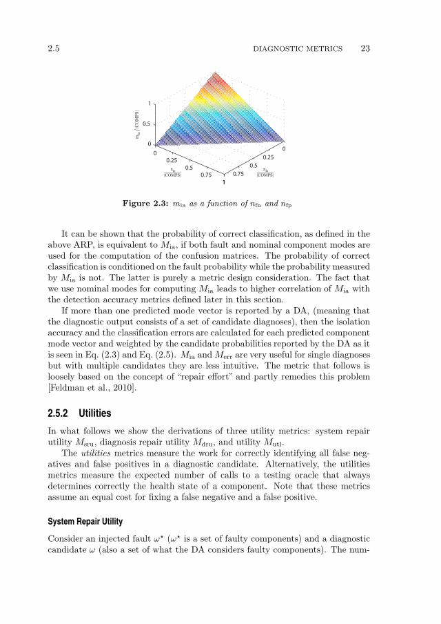
Eq. 2.7 defines a plane in the (nfn, nfp,mia)-space (cf. Fig 2.3).The mia metric “penalizes”a Diagnostic Algorithm (DA) for each misclassified
component. As it is visible from Fig. 2.3, the penalty is applied linearly.The isolation accuracy metricMia originates in the automotive industry [Com-
mittee E-32, 2008]. The Aerospace Recommended Practice (ARP) computes theclosely related probability of correct classification in the following way. For eachcomponent we compute a confusion matrix. The probability of correct classifica-tion is the sum of the main diagonal divided by the total number of classifications(cf. the referenced ARP [Committee E-32, 2008] for details and examples).
2.5 DIAGNOSTIC METRICS 23
0
0.25
0.5
0.75
1
00.25
0.50.75
1
0
0.5
1
nfn
|COMPS|
nfp
|COMPS|
mia
/ |C
OM
PS
|
Figure 2.3: mia as a function of nfn and nfp
It can be shown that the probability of correct classification, as defined in theabove ARP, is equivalent to Mia, if both fault and nominal component modes areused for the computation of the confusion matrices. The probability of correctclassification is conditioned on the fault probability while the probability measuredby Mia is not. The latter is purely a metric design consideration. The fact thatwe use nominal modes for computing Mia leads to higher correlation of Mia withthe detection accuracy metrics defined later in this section.
If more than one predicted mode vector is reported by a DA, (meaning thatthe diagnostic output consists of a set of candidate diagnoses), then the isolationaccuracy and the classification errors are calculated for each predicted componentmode vector and weighted by the candidate probabilities reported by the DA as itis seen in Eq. (2.3) and Eq. (2.5). Mia and Merr are very useful for single diagnosesbut with multiple candidates they are less intuitive. The metric that follows isloosely based on the concept of “repair effort” and partly remedies this problem[Feldman et al., 2010].
2.5.2 Utilities
In what follows we show the derivations of three utility metrics: system repairutility Msru, diagnosis repair utility Mdru, and utility Mutl.
The utilities metrics measure the work for correctly identifying all false neg-atives and false positives in a diagnostic candidate. Alternatively, the utilitiesmetrics measure the expected number of calls to a testing oracle that alwaysdetermines correctly the health state of a component. Note that these metricsassume an equal cost for fixing a false negative and a false positive.
System Repair Utility
Consider an injected fault ω⋆ (ω⋆ is a set of faulty components) and a diagnosticcandidate ω (also a set of what the DA considers faulty components). The num-
24 MODEL-BASED DIAGNOSIS 2.5
ber of truly faulty components that are improperly diagnosed by the diagnosticalgorithm as healthy (false negatives) is nfn = |ω⋆ \ ω| (cf. Fig. 2.2). In general adiagnostician has to perform extra work to verify a diagnostic candidate ω, whichmust be reflected in the system repair utility. We assume that he or she has accessto a test oracle that states if a component c is healthy or faulty.
We first determine what the expected number of tests a diagnostician has toperform to test all components in ω⋆ \ω (the false negatives) if the diagnosticianchooses untested components at random with uniform probability. In the worstcase, the diagnostician has to test all the remaining COMPS\ω components (thediagnostic algorithm has already determined the state of all components in ω).Consider the average situation. Recall that Nfn = |COMPS \ω|, where Nfn is thesize of the “population” of components to be tested.
The probability of observing s− 1 successes (faulty components) in k + s− 1trials (i.e., k oracle tests) is given by the direct application of the hypergeometricdistribution:
p(k, s− 1) =
(nfn
s−1
)(Nfn−nfn
k
)(
Nfn
k+s−1
) (2.8)
The probability p(k, s) of then observing a faulty component in the next oracletest is simply the number of remaining false negatives nfn− (s−1) divided by thesize of the remaining population (Nfn − (s+ k − 1)):
p(k, s) =nfn − s+ 1
Nfn − k − s+ 1(2.9)
and the probability of having exactly k oracle faults up to the s-th test, is thenthe product of these two probabilities:
p′(k, s, nfn, Nfn) =
(nfn
s−1
)(Nfn−nfn
k
)(nfn − s+ 1)
(Nfn
k+s−1
)(Nfn − k − s+ 1)
(2.10)
The formula above is the probability mass of the inverse hypergeometric distri-bution that, in our case, yields the probabilities for testing k healthy componentsbefore we find s faulty components out of the population (no repetitions). The ex-pected value E′[k] of p′(k, s, nfn, Nfn) (from the definition of a first central momentof a random variable) is:
E′[k] =
nfn∑
x=0
xp′(x, s, nfn, Nfn) (2.11)
Replacing p′(k, s, nfn, Nfn) in (2.11) and simplifying gives us the mean of theinverse hypergeometric distribution:3
E′[k] =s(Nfn − nfn)
nfn + 1(2.12)
3For a detailed derivation of the negative hypergeometric mean, cf. [Schuster and Sype, 1987].
2.5 DIAGNOSTIC METRICS 25
As we are interested in finding s = nfn faulty components, the expected valueE′(nfn, Nfn) becomes:
E′[k] =nfn(Nfn − nfn)
nfn + 1(2.13)
The expected number of tests E[tfn] (as opposed to the expected number of faultycomponents E′[k]) then becomes:
E[tfn] =nfn(Nfn − nfn)
nfn + 1+ nfn =
nfn(Nfn + 1)
nfn + 1(2.14)
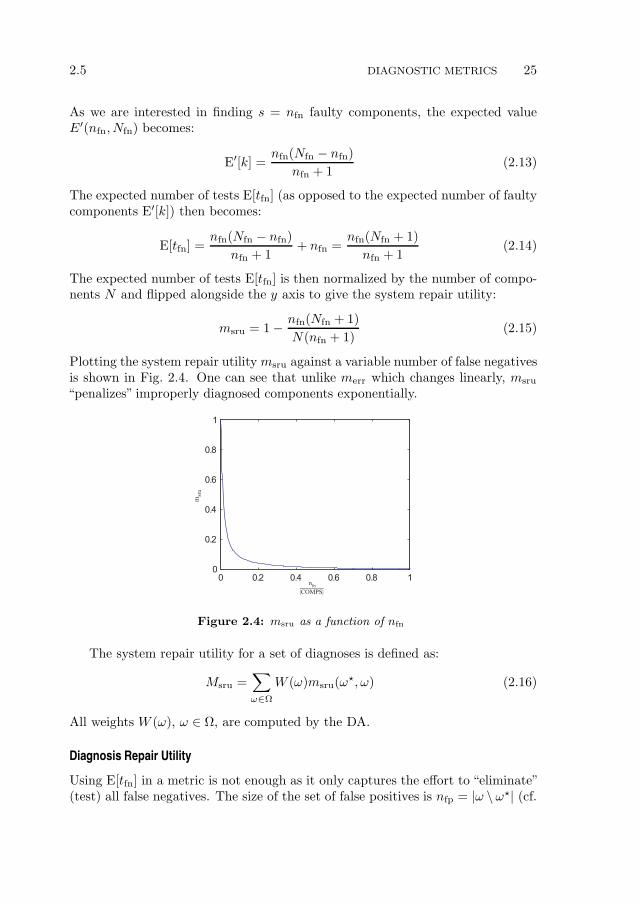
The expected number of tests E[tfn] is then normalized by the number of compo-nents N and flipped alongside the y axis to give the system repair utility:
msru = 1− nfn(Nfn + 1)
N(nfn + 1)(2.15)
Plotting the system repair utility msru against a variable number of false negativesis shown in Fig. 2.4. One can see that unlike merr which changes linearly, msru
“penalizes” improperly diagnosed components exponentially.
0 0.2 0.4 0.6 0.8 10
0.2
0.4
0.6
0.8
1
msr
u
nfn
|COMPS|
Figure 2.4: msru as a function of nfn
The system repair utility for a set of diagnoses is defined as:
Msru =∑
ω∈Ω
W (ω)msru(ω⋆, ω) (2.16)
All weights W (ω), ω ∈ Ω, are computed by the DA.
Diagnosis Repair Utility
Using E[tfn] in a metric is not enough as it only captures the effort to “eliminate”(test) all false negatives. The size of the set of false positives is nfp = |ω \ω⋆| (cf.

26 MODEL-BASED DIAGNOSIS 2.5
Fig. 2.2 and Table 2.3). To find all false positives, the diagnostician has to test inthe worst case all components in ω. Hence, the general population is Nfp = |ω|.Repeating the argument for E[tfn] we determine the expected number of tests fortesting all false positives E[tfp]:
E[tfp] =nfp(Nfp + 1)
nfp + 1(2.17)
Similarly, the diagnostic repair utility mdru is the normalized E[tfp]:
mdru = 1− nfp(Nfp + 1)
N(nfp + 1)(2.18)
The system repair utility for a set of diagnoses is defined as:
Mdru =∑
ω∈Ω
W (ω)mdru(ω⋆, ω) (2.19)
Utility
The utility metric (per candidate) is a combination of msru and mdru:
mutl = 1− E[tfn] + E[tfp]
N= 1− nfn(Nfn + 1)
N(nfn + 1)− nfp(Nfp + 1)
N(nfp + 1)(2.20)
The utility metric (per scenario4) is
Mutl =∑
ω∈Ω
W (ω)mutl(ω⋆, ω) (2.21)
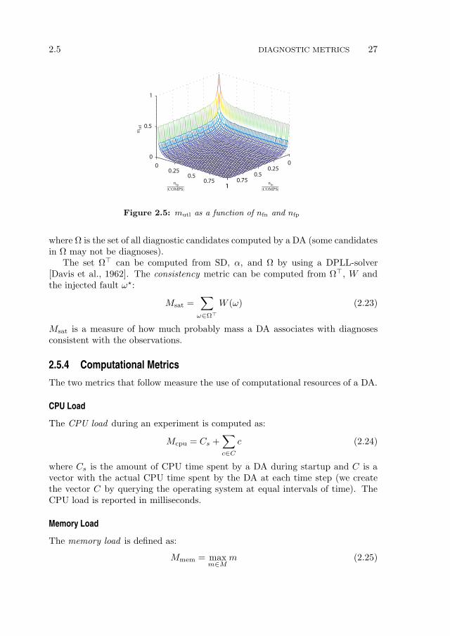
Figure 2.5 plots mutl for varying numbers of false negatives and false positives ina (symmetric) case where the cardinality of the injected fault is half the numberof components. Normally, the number of injected faulty components |ω⋆| is smallcompared to the total number of components f , which leads to an asymmetricmutl plot. In such cases, Nfp ≪ Nfn, hence the role of the false positives is small.In Fig. 2.5, there is a global optimum mutl = 1 for n = 0 and n = 0, i.e., allcomponents in ω are classified correctly.
2.5.3 Consistency
Consider a model SD and an observation α. The set of consistent diagnoses isdefined as:
Ω⊤ = ω ∈ Ω : SD ∧ α ∧ ω 6|=⊥ (2.22)
4We assume one observation per diagnostic scenario, unless specified otherwise.
2.5 DIAGNOSTIC METRICS 27
nfn
|COMPS|
nfp
|COMPS|
00.25
0.50.75
1
00.25
0.50.75
1
0
0.5
1
mu
tl
Figure 2.5: mutl as a function of nfn and nfp
where Ω is the set of all diagnostic candidates computed by a DA (some candidatesin Ω may not be diagnoses).
The set Ω⊤ can be computed from SD, α, and Ω by using a DPLL-solver[Davis et al., 1962]. The consistency metric can be computed from Ω⊤, W andthe injected fault ω⋆:
Msat =∑
ω∈Ω⊤
W (ω) (2.23)
Msat is a measure of how much probably mass a DA associates with diagnosesconsistent with the observations.
2.5.4 Computational Metrics
The two metrics that follow measure the use of computational resources of a DA.
CPU Load
The CPU load during an experiment is computed as:
Mcpu = Cs +∑
c∈C
c (2.24)
where Cs is the amount of CPU time spent by a DA during startup and C is avector with the actual CPU time spent by the DA at each time step (we createthe vector C by querying the operating system at equal intervals of time). TheCPU load is reported in milliseconds.
Memory Load
The memory load is defined as:
Mmem = maxm∈M
m (2.25)

28 MODEL-BASED DIAGNOSIS 2.5
where M is a vector with the maximum memory size allocated at each step of thediagnostic session. During an experiment, we create the vector M by repetitivelymeasuring the maximum memory consumption. The memory load is reported inKb.
2.5.5 System Metrics
For each system we consider a number of diagnostic scenarios. Throughout thisthesis, we assume that a diagnostic scenario consists of a single fault injection ω⋆
(a set of faulty components) that leads to a single observation α.The metrics Merr, Mia, Msru, Mdru, Mutl, Msat, and Mmem are based on a
single scenario. To receive “per system” results we combine the metrics of eachscenario using unweighted average. For example, if a system SD is tested withscenarios S = S1, S2, · · · , Sn, the “per system” utility of SD is computed as:
Mutl =∑
S∈S
1
|S|Mutl(SD, S) (2.26)
where Mutl(SD, S) is the “per scenario” utility of system SD and scenario S.The rest of the“per system”metrics (Merr, Mia, Msru, Mdru, Msat, and Mmem)
are defined in a way analogous to Mutl.
Chapter 3Approximate Model-Based
Diagnosis Using Greedy Stochastic
Search
In this chapter, we propose a StochAstic Fault diagnosis AlgoRIthm, called Sa-
fari, which trades off guarantees of computing minimal diagnoses for computa-tional efficiency. We empirically demonstrate, using the 74XXX and ISCAS85suites of benchmark combinatorial circuits, that Safari achieves several orders-of-magnitude speedup over two well-known deterministic algorithms, CDA∗ andHA∗, for multiple-fault diagnoses; further, Safari can compute a range of multi-ple-fault diagnoses that CDA∗ and HA∗ cannot. We also prove that Safari is op-timal for a range of propositional fault models, such as the widely-used weak-faultmodels (models with ignorance of abnormal behavior). We discuss the optimalityof Safari in a class of strong-fault circuit models with stuck-at failure modes.By modeling the algorithm itself as a Markov chain, we provide exact bounds onthe minimality of the diagnosis computed. Safari also displays strong anytimebehavior, and will return a diagnosis after any non-trivial inference time.
3.1 Introduction
Model-based diagnosis is an area of non-monotonic logic that uses a system model,together with observations about system behavior, to isolate sets of faulty compo-nents (diagnoses) that explain the observed behavior, according to some minimal-ity criterion. The standard MBD formalization [Reiter, 1987] frames a diagnosticproblem in terms of a set of logical clauses that include mode-variables describingthe nominal and fault status of system components; from this the diagnostic status
29
30 GREEDY STOCHASTIC SEARCH FOR MINIMAL DIAGNOSES 3.2
of the system can be computed given an observation of the system’s sensors. MBDprovides a sound and complete approach to enumerating multiple-fault diagnoses,and exact algorithms can guarantee finding a diagnosis optimal with respect tothe number of faulty components, probabilistic likelihood, etc.
The biggest challenge is the computational complexity of the MBD problem.The MBD problem of determining if there exists a diagnosis with at most kfaults is NP-hard for the arbitrary propositional models we consider in this thesis[Bylander et al., 1991; Friedrich et al., 1990]. Computing the set of all diagnosesis harder still, since there are possibly exponentially many such diagnoses. Sincealmost all proposed MBD algorithms have been complete and exact, with someauthors proposing possible trade-offs between completeness and faster consistencychecking by employing methods such as BCP [Williams and Ragno, 2007], thecomplexity problem still remains a major challenge to MBD.
To overcome this complexity problem, we propose a novel approximation ap-proach for multiple-fault diagnosis, based on a stochastic algorithm. Safari
(StochAstic Fault diagnosis AlgoRIthm) sacrifices guarantees of optimality, butfor diagnostic systems in which faults are described in terms of an arbitrary de-viation from nominal behavior Safari can compute diagnoses several orders ofmagnitude faster than competing algorithms.
Our contributions are as follows. (1) This chapter introduces an approximationalgorithm for computing diagnoses within an MBD framework, based on a greedystochastic algorithm. (2) We show that we can compute minimal-cardinality di-agnoses for weak fault models in poly-time (calling an incomplete SAT-solver thatimplements Boolean Constraint Propagation1 (BCP) only), and that more gen-eral frameworks (such as a sub-class of strong fault models) are also amenable tothis class of algorithm. (3) We model Safari search as a Markov chain to showthe performance and optimality trade-offs that the algorithm makes. (4) We ap-ply this algorithm to a suite of benchmark combinatorial circuits, demonstratingorder-of-magnitude speedup over two state-of-the-art deterministic algorithms,CDA∗ and HA∗, for multiple-fault diagnoses. (5) We compare the performanceof Safari against a range of Max-SAT algorithms for our benchmark problems.Our results indicate that, whereas the search complexity for the deterministicalgorithms tested increases exponentially with fault cardinality, the search com-plexity for this stochastic algorithm appears to be independent of fault cardinal-ity. Safari is of great practical significance, as it can compute a large fractionof minimal-cardinality diagnoses for discrete systems too large or complex to bediagnosed by existing deterministic algorithms.
3.2 Related Work
This chapter (1) generalizes Feldman et al. [2008c], (2) introduces important the-oretical results for strong-fault models, (3) extends the experimental results there,
1With formulae in CNF, BCP is implemented through the unit resolution rule.
3.2 RELATED WORK 31
and (4) provides a comprehensive optimality analysis of Safari.On a gross level, one can classify the types of algorithms that have been applied
to solve MBD as being based on search or compilation. The search algorithmstake as input the diagnostic model and an observation, and then search for a diag-nosis, which may be minimal with respect to some minimality criterion. Examplesof search algorithms include A∗-based algorithms, such as CDA∗ [Williams andRagno, 2007] and hitting set algorithms [Reiter, 1987]. Compilation algorithmspre-process the diagnostic model into a form that is more efficient for on-line diag-nostic inference. Examples of such algorithms include the ATMS [de Kleer, 1986a]and other prime-implicant methods [Kean and Tsiknis, 1993], DNNF [Darwiche,1998], and OBDD [Bryant, 1992]. To the best of our knowledge, all of these ap-proaches adopt exact methods to compute diagnoses; in contrast, Safari adoptsa stochastic approach to computing diagnoses.
At first glance, it seems like MBD could be efficiently solved using an encodingas a SAT [Jin et al., 2005], constraint satisfaction [Freuder et al., 1995] or Bayesiannetwork [Kask and Dechter, 1999] problem. However, one needs to take intoaccount the increase in formula size (over a direct MBD encoding), in addition tothe underconstrained nature of MBD problems.
Safari has resemblance to Max-SAT [Hoos and Stutzle, 2004] and we haveconducted extensive experimentation with both complete Max-SAT (partial andweighted) and Max-SAT based on Stochastic Local Search (SLS). Empirical evi-dence shows that although Max-SAT can compute diagnoses in many of the cases,the performance of Max-SAT degrades when increasing the circuit size or the car-dinality of the injected faults. In particular, Safari outperforms Max-SAT atleast an order-of-magnitude for the class of diagnostic problems we have consid-ered. In the case of SLS-based Max-SAT, the optimality of Max-SAT diagnosesis significantly worse than that of Safari.
We show that Safari exploits a particular property of MBD problems, calleddiagnostic continuity, which improves the optimality of Safari compared to, forexample, straightforward ALLSAT encodings [Jin et al., 2005]. We experimentallyconfirm this favorable performance and optimality of Safari. Although Safari
has close resemblance to Max-SAT, Safari exploits specific landscape propertiesof the diagnostic problems which allow (1) simple termination criteria and (2)optimality bounds. Due to the hybrid nature of Safari (the use of LTMS andSAT), Safari avoids getting stuck in local optima and performs better than Max-SAT based methods. Incorporating approaches from Max-SAT, and in particularSAPS [Hutter et al., 2002] in future versions of Safari may help in solving moregeneral abduction problems which may not expose the continuous properties ofthe models we have considered.
Stochastic algorithms have been discussed in the framework of constraint sat-isfaction [Freuder et al., 1995] and Bayesian network inference [Kask and Dechter,1999]. The latter two approaches can be used for solving suitably translated MBDproblems. It is often the case, though, that these encodings are more difficult forsearch than specialized ones.
32 GREEDY STOCHASTIC SEARCH FOR MINIMAL DIAGNOSES 3.2
MBD is an instance of constraint optimization, with particular constraints overfailure variables, as we will describe. MBD has developed algorithms to exploitthese domain properties, and our proposed approach differs significantly from al-most all MBD algorithms that appear in the literature. While most advancedMBD algorithms are deterministic, Safari borrows from SLS algorithms that,rather than backtracking, may randomly flip variable assignments to determinea satisfying assignment. Complete MBD algorithms typically make use of pref-erences, e.g., fault-mode probabilities, to improve search efficiency; Safari usesthis technique on top of its stochastic search over the space of diagnoses.
A closely-related diagnostic approach is that of Fijany et al. [2003], who mapthe minimal-hitting set problem into the problem of finding an assignment withbounded weight satisfying a monotone SAT problem, and then propose to useefficient SAT algorithms for computing diagnoses. The approach of Fijany et al.[2003] has shown speedups in comparison with other diagnosis algorithms; themain drawback is the number of extra variables and clauses that must be addedin the SAT encoding, which is even more significant for strong fault models andmulti-valued variables. In contrast, our approach works directly on the givendiagnosis model and requires no conversion to another representation.
Our work bears the closest resemblance to preference-based or Cost-BasedAbduction (CBA) [Charniak and Shimony, 1994; Santos Jr., 1994]. Of the algo-rithmic work in this area, the primary paper that adopts stochastic local searchis Abdelbar et al. [2006]. In this paper, Abdelbar et al. [2006] present a hybridtwo-stage method that is based on Iterated Local Search (ILS) and RepetitiveSimulated Annealing (RSA). The ILS stage of the algorithm uses a simple hill-climbing method (randomly flipping assumables) for the local search phase, andtabu search for the perturbation phase. RSA repeatedly applies Simulated An-nealing (SA), starting each time from a random initial state. The hybrid methodinitially starts from an arbitrary state, or a greedily-chosen state. It then ap-plies the ILS algorithm; if this algorithm fails to find the optimal solution after afixed number τ of hill-climbing steps2 or after a fixed number R of repetitions ofthe perturbation-local search cycle,3 ILS-based search is terminated and the RSAalgorithm is run until the optimal solution is found.
Our work differs from that of Abdelbar et al. [2006] in several ways. First,our initial state is generated using a random SAT solution. The hill-climbingphase that we use next is similar to that of Abdelbar et al. [2006]; however, werandomly restart should hill-climbing not identify a“better”diagnosis, rather thanapplying tabu-search or simulated annealing. Our approach is simpler than that
2Hill-climbing proceeds as follows: given a current state s with a cost of f(s), a neighbouringstate s′ is generated by flipping a randomly chosen assumable hypothesis. If f(s′) is better thanf(s), then s′ becomes the current state; otherwise, it is discarded. If τ iterations elapse withouta change in the current state, the local search exits.
3Perturbation-local search, starting from a current state s with a cost of f(s), randomlychooses an assumable variable h, and applies tabu-search to identify a better state by flippingh based on its tabu status.
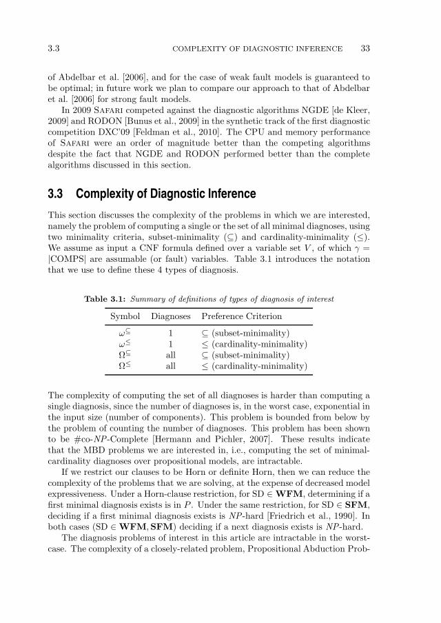
3.3 COMPLEXITY OF DIAGNOSTIC INFERENCE 33
of Abdelbar et al. [2006], and for the case of weak fault models is guaranteed tobe optimal; in future work we plan to compare our approach to that of Abdelbaret al. [2006] for strong fault models.
In 2009 Safari competed against the diagnostic algorithms NGDE [de Kleer,2009] and RODON [Bunus et al., 2009] in the synthetic track of the first diagnosticcompetition DXC’09 [Feldman et al., 2010]. The CPU and memory performanceof Safari were an order of magnitude better than the competing algorithmsdespite the fact that NGDE and RODON performed better than the completealgorithms discussed in this section.
3.3 Complexity of Diagnostic Inference
This section discusses the complexity of the problems in which we are interested,namely the problem of computing a single or the set of all minimal diagnoses, usingtwo minimality criteria, subset-minimality (⊆) and cardinality-minimality (≤).We assume as input a CNF formula defined over a variable set V , of which γ =|COMPS| are assumable (or fault) variables. Table 3.1 introduces the notationthat we use to define these 4 types of diagnosis.
Table 3.1: Summary of definitions of types of diagnosis of interest
Symbol Diagnoses Preference Criterion
ω⊆ 1 ⊆ (subset-minimality)ω≤ 1 ≤ (cardinality-minimality)Ω⊆ all ⊆ (subset-minimality)Ω≤ all ≤ (cardinality-minimality)
The complexity of computing the set of all diagnoses is harder than computing asingle diagnosis, since the number of diagnoses is, in the worst case, exponential inthe input size (number of components). This problem is bounded from below bythe problem of counting the number of diagnoses. This problem has been shownto be #co-NP-Complete [Hermann and Pichler, 2007]. These results indicatethat the MBD problems we are interested in, i.e., computing the set of minimal-cardinality diagnoses over propositional models, are intractable.
If we restrict our clauses to be Horn or definite Horn, then we can reduce thecomplexity of the problems that we are solving, at the expense of decreased modelexpressiveness. Under a Horn-clause restriction, for SD ∈WFM, determining if afirst minimal diagnosis exists is in P . Under the same restriction, for SD ∈ SFM,deciding if a first minimal diagnosis exists is NP-hard [Friedrich et al., 1990]. Inboth cases (SD ∈WFM,SFM) deciding if a next diagnosis exists is NP-hard.
The diagnosis problems of interest in this article are intractable in the worst-case. The complexity of a closely-related problem, Propositional Abduction Prob-
34 GREEDY STOCHASTIC SEARCH FOR MINIMAL DIAGNOSES 3.4
lems (PAPs), has been studied by Eiter and Gottlob [1995]. Eiter and Gottlobshow that for a propositional PAP, the problem of determining if a solution existsis ΣP
2 -complete. Computing a minimal diagnosis is a search problem, and hence itis more difficult to pose a decision question for proving complexity results. Con-sequently, one can just note that computing a diagnosis minimal with respectto ⊆ / ≤ requires O(log |COMPS|) calls to an NP oracle [Eiter and Gottlob,1995], asking the oracle at each step if a diagnosis containing at most k faultycomponents exists.
Results on abduction problems indicate that the task of approximate diagnosisis intractable. Roth [1996] has addressed the problems of abductive inference,and of approximating such inference. Roth focuses on counting the number ofsatisfying assignments for a range of AI problems, including some instances ofPAPs. In addition, Roth shows that approximating the number of satisfyingassignments for these problems is intractable.
Abdelbar [2004] has studied the complexity of approximating Horn abductionproblems, showing that even for a particular Horn restriction of the propositionalproblem of interest, the approximation problem is intractable. In particular, foran abduction problem with costs assigned to the assumables (which can be usedto model both the preference-orderings ⊆,≤), he has examined the complexity offinding the Least Cost Proof (LCP) for the evidence (OBS), where the cost of aproof is taken to be the sum of the costs of all hypotheses that must be assumedin order to complete the proof. For this problem he has shown that it is NP-hardto approximate an LCP within a fixed ratio r of the cost of an optimal solution,for any r > 0.
Safari approximates the intractable problems denoted in Table 3.1. We showthat for WFM, Safari can efficiently compute a single diagnosis that is mini-mal under ⊆ by using a satisfiability oracle. For SD ∈ SFM, Safari generatesa sound but possibly sub-optimal diagnosis (or set of diagnoses). We have re-ferred to papers indicating that it is intractable to approximate, within a fixedratio, a minimal diagnosis. In the following, we adopt a stochastic approach thatcannot provide fixed-ratio guarantees. However, Safari trades off optimality forefficiency and can compute most diagnoses with high likelihood.
3.4 Stochastic MBD Algorithm
In this section we discuss an algorithm for computing multiple-fault diagnosesusing stochastic search.
3.4.1 A Simple Example (Continued)
Consider the Boolean subtractor shown in Fig. 2.1, its weak-fault model SDw givenby (2.1), and the observation α4 from the preceding section. The four minimaldiagnoses associated to SDw ∧ α4 are: ω1 = ¬h1 ∧ h2 ∧ h3 ∧ h4 ∧ ¬h5 ∧ h6 ∧ h7,
3.4 STOCHASTIC MBD ALGORITHM 35
ω2 = h1 ∧ ¬h2 ∧ h3 ∧ h4 ∧ ¬h5 ∧ h6 ∧ h7, ω3 = ¬h1 ∧ h2 ∧ . . . ∧ h6 ∧ ¬h7, andω4 = h1 ∧ ¬h2 ∧ h3 ∧ . . . ∧ h6 ∧ ¬h7.
A naıve deterministic algorithm would check the consistency of all the 2|COMPS|
possible health assignments for a diagnostic problem, 128 in the case of our run-ning example. Furthermore, most deterministic algorithms first enumerate healthassignments of small cardinality but with high a priori probability, which ren-ders these algorithms impractical in situations when the minimal diagnosis is ofa higher cardinality. Such performance is not surprising even when using state-of-the art MBD algorithms which utilize, for example conflict learning, or partialcompilation, considering the bad worst-case complexity of finding all minimaldiagnoses (cf. Sec. 3.3).
In what follows, we will show a two-step diagnostic process that requires fewerconsistency checks. The first step involves finding a random non-minimal diag-nosis as a starting point (cf. Sec. 3.4.2 for details on computing random SATsolutions with equal likelyhood). The second step attempts to minimize the faultcardinality of this diagnosis by repeated modification of the diagnosis.
The first step is to find one random, possibly non-minimal diagnosis of SDw ∧α4. Such a diagnosis we can obtain from a classical DPLL solver after modifyingit in two ways: (1) not only determine if the instance is satisfiable but also extractthe satisfying solution and (2) find a random satisfiable solution every time thesolver is invoked. Both modifications are trivial, as DPLL solvers typically storetheir current variable assignments and it is easy to choose a random variable andvalue when branching instead of deterministic ones. The latter modification maypossibly harm a DPLL variable or value selection heuristics, but later in thischapter we will see that this is of no concern for the type of problems we areconsidering as diagnostic systems are typically underconstrained.
In the subtractor example we call the DPLL solver with SDw ∧ α4 as aninput and we consider the random solution (and obviously a diagnosis) ω5 =¬h1 ∧ h2 ∧ ¬h3 ∧ h4 ∧ h5 ∧ ¬h6 ∧ ¬h7 (|ω5| = 4). In the second step of ourstochastic algorithm, we will try to minimize ω5 by repetitively choosing a randomnegative literal, “flipping” its value to positive (thus obtaining a candidate with asmaller number of faults), and calling the DPLL solver. If the new candidate is adiagnosis, we will try to improve further this newly discovered diagnosis, otherwisewe will mark the attempt a “failure” and choose another negative literal. Aftersome constant number of “failures” (two in this example), we will terminate thesearch and will store the best diagnosis discovered so far in the process.
After changing the sign of ¬h7 in ω5 we discover that the new health assign-ment is not consistent with SDw∧α4, hence it is not a diagnosis and we discard it.Instead, the algorithm attempts changing ¬h6 to h6 in ω5, this time successfullyobtaining a new diagnosis ω6 = ¬h1 ∧ h2 ∧¬h3 ∧ h4 ∧ h5 ∧h6 ∧¬h7 of cardinality3. Next the algorithm tries to find a diagnosis of even smaller cardinality by ran-domly choosing ¬h1 and ¬h7 in ω6, respectively, and trying to change their sign,but both attempts return an inconsistency. Hence the “climb” is aborted and ω6
is stored as the current best diagnosis.
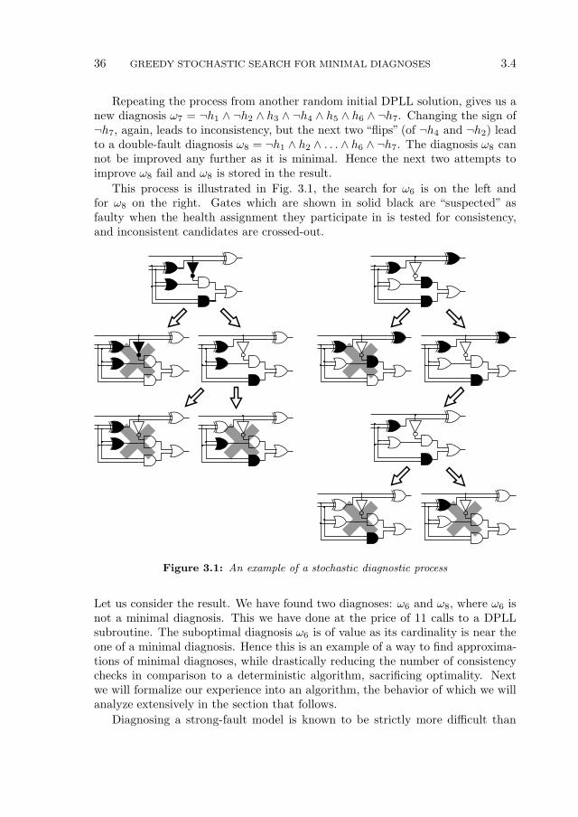
36 GREEDY STOCHASTIC SEARCH FOR MINIMAL DIAGNOSES 3.4
Repeating the process from another random initial DPLL solution, gives us anew diagnosis ω7 = ¬h1 ∧ ¬h2 ∧ h3 ∧ ¬h4 ∧ h5 ∧ h6 ∧ ¬h7. Changing the sign of¬h7, again, leads to inconsistency, but the next two “flips” (of ¬h4 and ¬h2) leadto a double-fault diagnosis ω8 = ¬h1 ∧ h2 ∧ . . . ∧ h6 ∧ ¬h7. The diagnosis ω8 cannot be improved any further as it is minimal. Hence the next two attempts toimprove ω8 fail and ω8 is stored in the result.
This process is illustrated in Fig. 3.1, the search for ω6 is on the left andfor ω8 on the right. Gates which are shown in solid black are “suspected” asfaulty when the health assignment they participate in is tested for consistency,and inconsistent candidates are crossed-out.
Figure 3.1: An example of a stochastic diagnostic process
Let us consider the result. We have found two diagnoses: ω6 and ω8, where ω6 isnot a minimal diagnosis. This we have done at the price of 11 calls to a DPLLsubroutine. The suboptimal diagnosis ω6 is of value as its cardinality is near theone of a minimal diagnosis. Hence this is an example of a way to find approxima-tions of minimal diagnoses, while drastically reducing the number of consistencychecks in comparison to a deterministic algorithm, sacrificing optimality. Nextwe will formalize our experience into an algorithm, the behavior of which we willanalyze extensively in the section that follows.
Diagnosing a strong-fault model is known to be strictly more difficult than

3.4 STOCHASTIC MBD ALGORITHM 37
a weak-fault model [Friedrich et al., 1990]. In many diagnostic instances thisproblem is alleviated by the fact that there exist, although without a guarantee,continuities in the diagnostic search space similar to the one in the weak-faultmodels. Let us discuss the process of finding a minimal diagnosis of the sub-tractor’s strong-fault model SDs and the observation α2 (both from Sec. 2.1.1).
h7
3
h7
3
3
3
3 3
h7
3
h7
3
3
3
3
3
3
h6
3
3
3
h6
3
3
h6
7
7
3
h6
3
3
7
h5
7
h5
7
7
7
7
7
h5
7
h5
7
7 7
7
7
h4
7
h4
3
3
3
3 3
h4
7
h4
7
3
3
3
3
h3
7
7
3
h3
7
3
3
h3
3
7
3
h3
7
3
7
h2
7
h2
7
7
7
7 7
h2
7
h2
7
7
7
7
7
3
h1 h1
3
3
3
3
3
3
h1 h1
3
3 3
3
3
ω9
ω13
ω14
ω9
ω11
ω14
ω10
ω12
ω14
ω10
ω13
ω14
Figure 3.2: Diagnoses of a strong-fault model
Figure 3.2 illustrates the notion of continuity in a strong-fault model. In the fourscenarios, a diagnostician starts from ω14 and improves the cardinality by changingthe sign of a single literal in each diagnosis. At each step we receive one of the sixdistinct diagnoses of SDs ∧ α2 (these are ω9, ω10, . . . , ω14 as shown in Fig. 3.2).Of these six diagnoses only ω9 and ω10 are minimal such that |ω9| = |ω10| = 3. Itis visible in Fig. 3.2 that component variables h2 and h5 are false in all diagnoses,while h1 and h7 are always true (healthy). Hence, any satisfying assignment ofSDs∧α2 would contain h1∧¬h2∧¬h5∧h7. Starting from the maximal-cardinalitydiagnosis ω14 (note that the all-faulty assignment in a strong-fault model is notnecessarily a diagnosis), we must “flip” the variables h3, h4, and h6 in order toreach the two minimal diagnoses. The key insight is that, as shown in Fig. 3.2,this is always possible by “flipping” a single literal at a time from health to faultyand receiving another consistent assignment (diagnosis).
In what follows we will formalize our experience so far in a stochastic algorithmfor finding minimal diagnoses.
3.4.2 A Greedy Stochastic Algorithm
The randomized search process performed by Safari (cf. Alg. 1) has two param-eters, M and N . There are N independent searches that start from randomlygenerated starting points. The algorithm tries to improve the cardinality of theinitial diagnoses (while preserving their consistency) by randomly “flipping” faultliterals. The change of a sign of literal is done in one direction only: from faultyto healthy.
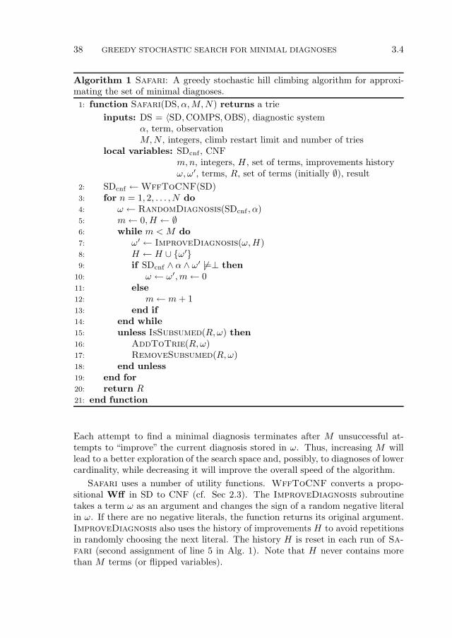
38 GREEDY STOCHASTIC SEARCH FOR MINIMAL DIAGNOSES 3.4
Algorithm 1 Safari: A greedy stochastic hill climbing algorithm for approxi-mating the set of minimal diagnoses.
1: function Safari(DS, α,M,N) returns a trie
inputs: DS = 〈SD,COMPS,OBS〉, diagnostic systemα, term, observationM,N , integers, climb restart limit and number of tries
local variables: SDcnf , CNFm,n, integers, H , set of terms, improvements historyω, ω′, terms, R, set of terms (initially ∅), result
2: SDcnf ←WffToCNF(SD)3: for n = 1, 2, . . . , N do
4: ω ← RandomDiagnosis(SDcnf , α)5: m← 0, H ← ∅6: while m < M do
7: ω′ ← ImproveDiagnosis(ω,H)8: H ← H ∪ ω′9: if SDcnf ∧ α ∧ ω′ 6|=⊥ then
10: ω ← ω′,m← 011: else
12: m← m+ 113: end if
14: end while
15: unless IsSubsumed(R,ω) then
16: AddToTrie(R,ω)17: RemoveSubsumed(R,ω)18: end unless
19: end for
20: return R21: end function
Each attempt to find a minimal diagnosis terminates after M unsuccessful at-tempts to “improve” the current diagnosis stored in ω. Thus, increasing M willlead to a better exploration of the search space and, possibly, to diagnoses of lowercardinality, while decreasing it will improve the overall speed of the algorithm.
Safari uses a number of utility functions. WffToCNF converts a propo-sitional Wff in SD to CNF (cf. Sec 2.3). The ImproveDiagnosis subroutinetakes a term ω as an argument and changes the sign of a random negative literalin ω. If there are no negative literals, the function returns its original argument.ImproveDiagnosis also uses the history of improvements H to avoid repetitionsin randomly choosing the next literal. The history H is reset in each run of Sa-
fari (second assignment of line 5 in Alg. 1). Note that H never contains morethan M terms (or flipped variables).
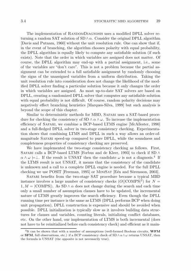
3.4 STOCHASTIC MBD ALGORITHM 39
The implementation of RandomDiagnosis uses a modified DPLL solver re-turning a random SAT solution of SD∧α. Consider the original DPLL algorithm[Davis and Putnam, 1960] without the unit resolution rule. One can show that if,in the event of branching, the algorithm chooses polarity with equal probability,the DPLL algorithm is equally likely to compute any satisfiable solution (if suchexists). Note that the order in which variables are assigned does not matter. Ofcourse, the DPLL algorithm may end-up with a partial assignment, i.e., someof the variables are “don’t care”. This is not a problem because the partial as-signment can be extended to a full satisfiable assignment by randomly choosingthe signs of the unassigned variables from a uniform distribution. Taking theunit resolution rule into consideration does not change the likelihood of the mod-ified DPLL solver finding a particular solution because it only changes the orderin which variables are assigned. As most up-to-date SAT solvers are based onDPLL, creating a randomized DPLL solver that computes any satisfiable solutionwith equal probability is not difficult. Of course, random polarity decisions maynegatively effect branching heuristics [Marques-Silva, 1999] but such analysis isbeyond the scope of this chapter.
Similar to deterministic methods for MBD, Safari uses a SAT-based proce-dure for checking the consistency of SD ∧ α ∧ ω. To increase the implementationefficiency of Safari, we combine a BCP-based LTMS engine [McAllester, 1990]and a full-fledged DPLL solver in two-stage consistency checking. Experimenta-tion shows that combining LTMS and DPLL in such a way allows an order-of-magnitude Safari speed-up compared to pure DPLL, while the soundness andcompleteness properties of consistency checking are preserved.
We have implemented the two-stage consistency checking as follows. First,Safari calls a BCP-based LTMS [Forbus and de Kleer, 1993] to check if SD ∧α ∧ ω |=⊥. If the result is UNSAT then the candidate ω is not a diagnosis.4 Ifthe LTMS result is not UNSAT, it means that the consistency of the candidateis unknown and a call to a complete DPLL engine is needed. For the full DPLLchecking we use POSIT [Freeman, 1995] or MiniSat [Een and Sorensson, 2003].
Safari benefits from the two-stage SAT procedure because a typical MBDinstance involves a large number of consistency checks (O(|COMPS|2) for N =1,M = |COMPS|). As SD ∧ α does not change during the search and each timeonly a small number of assumption clauses have to be updated, the incrementalnature of LTMS greatly improves the search efficiency. Even though the DPLLrunning time per instance is the same as LTMS (DPLL performs BCP when doingunit propagation), DPLL construction is expensive and should be avoided whenpossible. DPLL initialization is typically slow as it involves building data struc-tures for clauses and variables, counting literals, initializing conflict databases,etc. On the other hand, our implementation of LTMS is both incremental (doesnot have to be reinitialized before each consistency check) and efficient as it main-
4It can be shown that with a number of assumptions (well-formed Boolean circuits, WFM
or SFM, full observations, etc.) if a BCP consistency check of SD∧α∧ω returns UNSAT, thenthe formula is UNSAT (the opposite is not necessarily true).

40 GREEDY STOCHASTIC SEARCH FOR MINIMAL DIAGNOSES 3.4
tains only counters for each clause. Each counter keeps the number of unassignedliterals. Assigning a value to a variable requires decrementing some or all of theclause counters. If a counter becomes zero, a contradiction handler is signaled.
There is no guarantee that two diagnostic searches, starting from randomdiagnoses, would not lead to the same minimal diagnosis. To prevent this, westore the generated diagnoses in a trie R [Forbus and de Kleer, 1993], from whichit is straightforward to extract the resulting diagnoses by recursively visiting itsnodes. A diagnosis ω is added to the trie R by the function AddToTrie, iffno subsuming diagnosis is contained in R (the IsSubsumed subroutine checks onthat condition). After adding a diagnosis ω to the resulting trie R, all diagnosescontained in R and subsumed by ω are removed by a call to RemoveSubsumed.
3.4.3 Basic Properties of the Greedy Stochastic Search
Before we continue with the topics of completeness and optimality we show thatSafari is sound.
Lemma 2 (Soundness). All diagnoses returned by Safari are sound.
Proof (Sketch). The consistency check in line 8 of Alg. 1 guarantees that onlyterms ω for which it holds that SD∧α ∧ ω 6|=⊥ will be added to the result set R.According to Def. 5 these terms ω are diagnoses.
One of the key factors in the success of the proposed algorithm is the exploitationof the continuity of the search-space of diagnosis models, where by continuity wemean that we can monotonically reduce the cardinality of a non-minimal diagno-sis. Through the exploitation of this continuity property, Safari can be config-ured to guarantee finding a minimal diagnosis in weak fault models in polynomialnumber of calls to a satisfiability oracle.
The hypothesis which comes next is well studied in prior work [de Kleer et al.,1992a] as it determines the conditions in which minimal diagnoses represent alldiagnoses of a model and an observation. This chapter is interested in the hy-pothesis from the computational viewpoint: it defines a class of models for whichit is possible to establish a theoretical bound on the optimality and performanceof Safari.
Hypothesis 1 (Minimal Diagnosis Hypothesis). Let DS = 〈SD,COMPS,OBS〉be a diagnostic system and ω′ a diagnosis for an arbitrary observation α. TheMinimal Diagnosis Hypothesis (MDH) holds in DS iff for any health assignmentω such that Lit−(ω) ⊃ Lit−(ω′), it holds that ω is also a diagnosis.
It is easy to show that MDH holds for all weak-fault models. There are othertheories SD 6∈ WFM for which MDH holds (e.g., one can directly constructa theory as a conjunction of terms for which MDH holds). Unfortunately, nonecessary condition is known for MDH to hold in an arbitrary SD. The lemmawhich comes next is a direct consequence of MDH and weak-fault models.

3.4 STOCHASTIC MBD ALGORITHM 41
Lemma 3. Given a diagnostic system DS = 〈SD, COMPS, OBS〉, SD ∈WFM,and a diagnosis ω for some observation α, it follows that ω is non-minimal iffanother diagnosis ω′ can be obtained by changing the sign of exactly one negativeliteral in ω.
Proof (Sketch). From Def. 2 and SD ∈ WFM, it follows that if ω is a minimaldiagnosis, any diagnosis ω′ obtained by flipping one positive literal in ω is alsoa diagnosis. Applying the argument in the other direction gives us the abovestatement.
Safari operates by performing subset flips on non-minimal diagnoses, attemptingto compute minimal diagnoses. We next formalize this notion of flips, in order tocharacterize when Safari will be able to compute a minimal diagnosis.
Definition 11 (Subset Flip Φ⇓). Given a diagnostic system DS = 〈SD, COMPS,OBS〉 and a health assignment ω with a non-empty set of negative literals (Lit−(ω)6= ∅), a subset flip Φ⇓ turns one of the negative literals in ω to a positive literal,i.e., it creates a health assignment ω′ with one more positive literal.
We next characterize flips based on whether they produce consistent models afterthe flip.
Definition 12 (Valid Subset Flip). Given a system DS = 〈SD, COMPS, OBS〉,an observation α, and a non-minimal diagnosis ω, a subset flip Φ⇓ is valid iff Φ⇓
creates a health assignment that is also a diagnosis.
Given these notions, we can define continuity of the diagnosis search space interms of literal flipping.
Definition 13 (Continuity). A system model SD and an observation α satisfythe continuity property with respect to the set of diagnoses Ω⊆(SD ∧ α), iff forany diagnosis ωk ∈ Ω(SD∧α) there exists a sequence Φ = 〈ω1, ω2, · · · , ωk−1, ωk,ωk+1, · · · , ωn〉, such that for i = 1, 2, · · · , n − 1, it is possible to go from ωi toωi+1 via a valid subset flip, ωi ∈ Ω(SD ∧ α), and ωn ∈ Ω⊆(SD ∧ α).
Given this definition of continuity, we can easily show the following two lemmata:
Lemma 4. If SD satisfies MDH, then it satisfies the continuity property.
Proof. Follows directly from Hypothesis 1 and Def 13.
Lemma 5. SD ∈WFM satisfies the continuity property.
Proof (Sketch). It is straightforward to show that if SD ∈WFM then SD satisfiesMDH. Then from Lemma 4 it follows that SD satisfies the continuous property.

42 GREEDY STOCHASTIC SEARCH FOR MINIMAL DIAGNOSES 3.4
Our greedy algorithm starts with an initial diagnosis and then randomly flipsfaulty assumable variables. We now use the MDH property to show that, startingwith a non-minimal diagnosis ω, the greedy stochastic diagnosis algorithm canmonotonically reduce the size of the“seed”diagnosis to obtain a minimal diagnosisthrough appropriately flipping a fault variable from faulty to healthy; if we viewthis flipping as search, then this search is continuous in the diagnosis space.
Proposition 1. Given a diagnostic system DS = 〈SD,COMPS,OBS〉, an obser-vation α, and SD ∈WFM, Safari configured with M = |COMPS| and N = 1returns one minimal diagnosis.
Proof. The diagnosis improvement loop starts, in the worst case, from a healthassignment ω which is a conjunction of negative literals only. Necessarily, in thiscase, ω is a diagnosis as SD ∈WFM. A diagnosis ω′ that is subsumed by ω wouldbe found with at most M consistency checks (provided that ω′ exists) as M is setto be equal to the number of literals in ω and there are no repetitions in randomlychoosing of which literal to flip next. If, after trying all the negative literals in ω,there is no diagnosis, then from Lemma 3 it follows that ω is a minimal diagnosis.
Through a simple inductive argument, we can continue this process until weobtain a minimal diagnosis.
From Proposition 1 it follows that there is an upper bound of O(|COMPS|2)consistency checks for finding a single minimal diagnosis. In most of the practicalcases, however, we are interested in finding an approximation to all minimal-cardinality diagnoses. As a result the complexity of the optimally configuredSafari algorithm becomes O(|COMPS|2S), where S is the number of minimal-cardinality diagnoses for the given observation. Section 3.6 discusses in moredetail the computation of multiple minimal-cardinality diagnoses.
The number of assumable variables in a system of practical significance mayexceed thousands, rendering an optimally configured Safari computationally tooexpensive. In Sec 3.5 we will see that while it is more computationally efficient toconfigure M < |COMPS|, it is still possible to find a minimal diagnosis with highprobability.
It is simple to show that flip-based search algorithms are complete for con-tinuous diagnosis search spaces given weak fault models, i.e., SD ∈ WFM, andmodels that follow MDH, i.e., Lemma 3. We can formally characterize the guaran-tee of finding a minimal diagnosis with Safari in terms of a continuous diagnosisspace. Note that this is a sufficient, but not necessary, condition; for example, wemay configure Safari to flip multiple literals at a time to circumvent problemsof getting trapped in discontinuous diagnosis spaces.
Theorem 1. Given a diagnostic system DS = 〈SD,COMPS,OBS〉, and a startingdiagnosis ω, Safari configured with M = |COMPS| and N = 1 is guaranteed tocompute a minimal diagnosis if the diagnosis space is continuous.

3.4 STOCHASTIC MBD ALGORITHM 43
Proof. Given an initial diagnosis ω, Safari attempts to compute a minimal di-agnosis by performing subset flips. If the diagnosis space is continuous, then weknow that there exists a sequence of valid flips leading to a minimal diagnosis.Hence Safari is guaranteed to find a minimal diagnosis from ω.
Finally, we show that Safari is guaranteed to compute all minimal diagnoses.
Theorem 2. Consider a diagnostic system DS = 〈SD,COMPS,OBS〉, an obser-vation α, and a continuous diagnosis space Ω(SD, α). We denote the event ofSafari computing all minimal diagnoses of SD ∧ α after N runs with Υ(N). Itfollows that limN→∞ Pr(Υ(N)) = 1.
Proof (Sketch). Since (1) the search space is continuous, (2) at each step there is anon-zero probability of flipping any unflipped literal, and (3) there is a polynomialupper bound of steps (|COMPS|) for computing a diagnosis, Safari can computeany non-minimal diagnosis with non-zero probability. Hence as N →∞, Safari
will compute all minimal diagnoses.
3.4.4 Complexity of Inference Using Greedy Stochastic Search
We next look at the complexity of Safari, and its stochastic approach to comput-ing sound but incomplete diagnoses. We show that the primary determinant ofthe inference complexity is the consistency checking. Safari randomly computesa partial assignment π, and then checks if π can be extended to create a satisfyingassignment during each consistency check, i.e., it checks the consistency of π withSD. This is solving the satisfiability problem (SAT), which is NP-complete [Cook,1971]. We will show how we can use incomplete satisfiability checking to reducethis complexity, at the cost of completeness guarantees.
In the following, we call Ψ the complexity of a consistency check, and assumethat there are γ components that can fail, i.e., γ = |COMPS|.
Lemma 6. Given a diagnostic system DS = 〈SD,COMPS,OBS〉 with SD ∈WFM, the worst-case complexity of finding any minimal diagnosis is O(γ2Ψ),where Ψ is the cost of a consistency check.
Proof. From Proposition 1 it follows that there is an upper bound of γ consistencychecks for finding a single minimal diagnosis, since at each step (there is a max-imum of γ steps for computing the “all healthy” diagnosis), the algorithm mustflip at most γ literals. The total complexity is hence O(γ2Ψ), since we perform aconsistency check after each flip.
The complexity of BCP is well-known allowing us to get more precise bounds onthe worst-case complexity of computing one minimal-diagnosis with Safari. Inwhat follows we will assume that SD is in CNF (cf. Sec. 2.3).

44 GREEDY STOCHASTIC SEARCH FOR MINIMAL DIAGNOSES 3.5
Lemma 7. Given a diagnostic system DS = 〈SD,COMPS,OBS〉, SD ∈WFM,and SD having c clauses and n variables, the worst-case complexity under WFM
of finding any minimal diagnosis is O(γ2cn) when using BCP for consistencychecks.5
Proof (Sketch). An implementation of BCP [Forbus and de Kleer, 1993] maintainsa total of c counters for the number of unsatisfied literals in each clause. Aconsistency check requires decrementing some or all counters for each of the nvariables in SD. This gives us an upper bound of O(cn) on the execution timeof BCP. Combining the complexity of BCP with Lemma 6 gives us the desiredresult.
In most practical cases, however, we are interested in finding an approximationto all minimal-cardinality diagnoses. As a result the complexity of the optimally
configured Safari algorithm becomes O(γ(|ω|γ
)Ψ
), where |ω| is the cardinality
of the minimal-cardinality diagnoses for the given observation (cf. Sec. 3.7.7).
3.5 Optimality Analysis (Single Diagnosis)
In contrast to deterministic algorithms, in the Safari algorithm there is no ab-solute guarantee that the optimum solution (minimal diagnosis) is found for ar-bitrary values of the configuration parameter M (M < |COMPS|). Below we willprovide an intuition behind the performance of the Safari algorithm by meansof an approximate, analytical model that estimates the probability of reaching adiagnostic solution of specific minimality.
3.5.1 Optimality of SAFARI in Weak-Fault Models
We will start by considering a single run of the algorithm without retries wherewe will assume the existence of only one minimal diagnosis. Next, we will extendthe model by considering retries.
Basic Model
Consider a diagnostic system DS = 〈SD,COMPS,OBS〉 such that SD ∈ WFM
and an observation α such that α manifests only one minimal diagnosis ω. Forthe argument that follows we will configure Safari with M = 1, N = 1, and wewill assume that the starting solution is the trivial “all faulty” diagnosis.
When Safari randomly chooses a faulty variable and flips it, we will be sayingthat it is a “success” if the new candidate is a diagnosis and, a “failure” otherwise.Let k denote the number of steps that the algorithm successfully traverses in thedirection of the minimal diagnosis of cardinality |ω|. Thus k also measures the
5More efficient implementations of BCP exist [Zhang and Stickel, 1996].
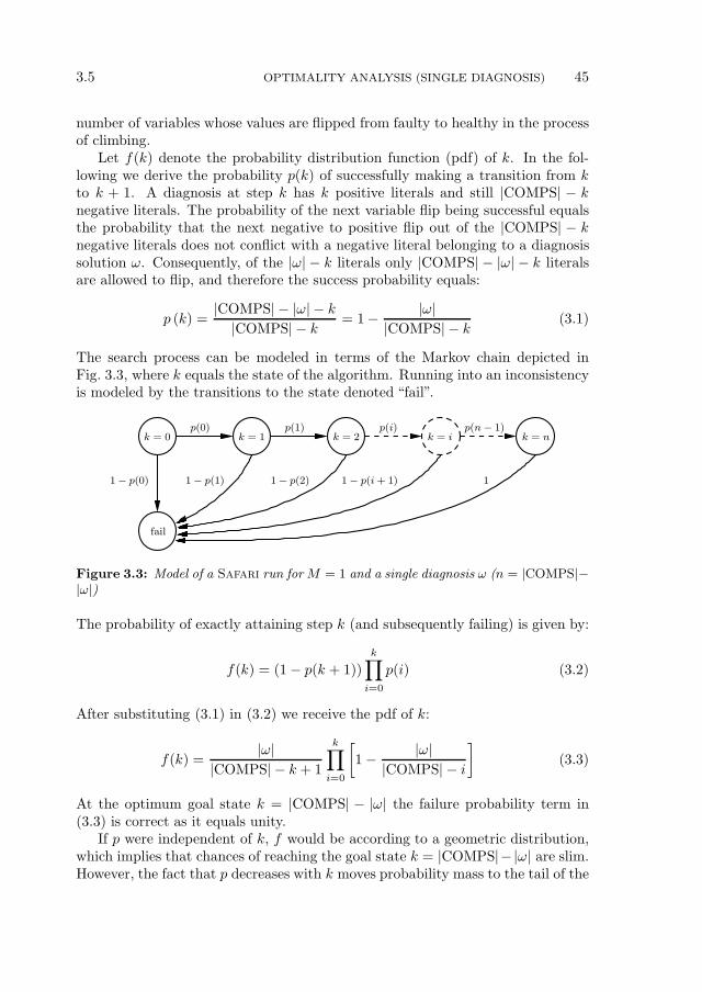
3.5 OPTIMALITY ANALYSIS (SINGLE DIAGNOSIS) 45
number of variables whose values are flipped from faulty to healthy in the processof climbing.
Let f(k) denote the probability distribution function (pdf) of k. In the fol-lowing we derive the probability p(k) of successfully making a transition from kto k + 1. A diagnosis at step k has k positive literals and still |COMPS| − knegative literals. The probability of the next variable flip being successful equalsthe probability that the next negative to positive flip out of the |COMPS| − knegative literals does not conflict with a negative literal belonging to a diagnosissolution ω. Consequently, of the |ω| − k literals only |COMPS| − |ω| − k literalsare allowed to flip, and therefore the success probability equals:
p (k) =|COMPS| − |ω| − k|COMPS| − k = 1− |ω|
|COMPS| − k (3.1)
The search process can be modeled in terms of the Markov chain depicted inFig. 3.3, where k equals the state of the algorithm. Running into an inconsistencyis modeled by the transitions to the state denoted “fail”.
fail
p(0) p(1) p(i) p(n − 1)
1 − p(0) 1 − p(1) 1 − p(2) 1 − p(i + 1)
k = 0 k = 1 k = 2 k = i k = n
1
Figure 3.3: Model of a Safari run for M = 1 and a single diagnosis ω (n = |COMPS|−|ω|)
The probability of exactly attaining step k (and subsequently failing) is given by:
f(k) = (1− p(k + 1))
k∏
i=0
p(i) (3.2)
After substituting (3.1) in (3.2) we receive the pdf of k:
f(k) =|ω|
|COMPS| − k + 1
k∏
i=0
[1− |ω||COMPS| − i
](3.3)
At the optimum goal state k = |COMPS| − |ω| the failure probability term in(3.3) is correct as it equals unity.
If p were independent of k, f would be according to a geometric distribution,which implies that chances of reaching the goal state k = |COMPS|− |ω| are slim.However, the fact that p decreases with k moves probability mass to the tail of the
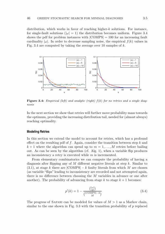
46 GREEDY STOCHASTIC SEARCH FOR MINIMAL DIAGNOSES 3.5
distribution, which works in favor of reaching higher-k solutions. For instance,for single-fault solutions (|ω| = 1) the distribution becomes uniform. Figure 3.4shows the pdf for problem instances with |COMPS| = 100 for an increasing faultcardinality |ω|. In order to decrease sampling noise, the empirical f(k) values inFig. 3.4 are computed by taking the average over 10 samples of k.
0 20 40 60 80 1000
0.02
0.04
0.06
0.08
0.1
k
f(k)
0 20 40 60 80 1000
0.02
0.04
0.06
0.08
0.1
kf(
k)
|ω| = 1
|ω| = 5
|ω| = 10
|ω| = 1
|ω| = 5
|ω| = 10
Figure 3.4: Empirical (left) and analytic (right) f(k) for no retries and a single diag-nosis
In the next section we show that retries will further move probability mass towardsthe optimum, providing the increasing distribution tail, needed for (almost always)reaching optimality.
Modeling Retries
In this section we extend the model to account for retries, which has a profoundeffect on the resulting pdf of f . Again, consider the transition between step k andk + 1 where the algorithm can spend up to m = 1, . . . ,M retries before bailingout. As can be seen by the algorithm (cf. Alg. 1), when a variable flip producesan inconsistency a retry is executed while m is incremented.
From elementary combinatorics we can compute the probability of having adiagnosis after flipping any of M different negative literals at step k. Similar to(3.1), at stage k there are |COMPS| − k faulty literals from which M are chosen(as variable “flips” leading to inconsistency are recorded and not attempted again,there is no difference between choosing the M variables in advance or one afteranother). The probability of advancing from stage k to stage k + 1 becomes:
p′(k) = 1−(|ω|M
)(|COMPS|−k
M
) (3.4)
The progress of Safari can be modeled for values of M > 1 as a Markov chain,similar to the one shown in Fig. 3.3 with the transition probability of p replaced
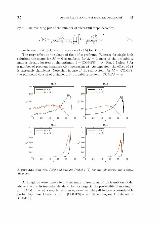
3.5 OPTIMALITY ANALYSIS (SINGLE DIAGNOSIS) 47
by p′. The resulting pdf of the number of successful steps becomes:
f ′(k) =
(|ω|M
)(|COMPS|−k+1
M
)k∏
i=0
[1−
(|ω|M
)(|COMPS|−i
M
)]
(3.5)
It can be seen that (3.3) is a private case of (3.5) for M = 1.
The retry effect on the shape of the pdf is profound. Whereas for single-faultsolutions the shape for M = 0 is uniform, for M = 1 most of the probabilitymass is already located at the optimum k = |COMPS| − |ω|. Fig. 3.5 plots f fora number of problem instances with increasing M . As expected, the effect of Mis extremely significant. Note that in case of the real system, for M = |COMPS|the pdf would consist of a single, unit probability spike at |COMPS| − |ω|.
0 20 40 60 80 1000
0.01
0.02
0.03
0.04
k
f’ (k)
M = 2
0 20 40 60 80 1000
0.01
0.02
0.03
0.04
k
f’ (k)
M = 2
0 20 40 60 80 1000
0.02
0.04
0.06
0.08
0.1
0.12
k
f’ (k)
M = 4
0 20 40 60 80 1000
0.02
0.04
0.06
0.08
0.1
0.12
k
f’ (k)
M = 4
|ω| = 5
|ω| = 10
|ω| = 5
|ω| = 10
|ω| = 5
|ω| = 10
|ω| = 5
|ω| = 10
Figure 3.5: Empirical (left) and analytic (right) f ′(k) for multiple retries and a singlediagnosis
Although we were unable to find an analytic treatment of the transition modelabove, the graphs immediately show that for largeM the probability of moving tok = |COMPS|− |ω| is very large. Hence, we expect the pdf to have a considerableprobability mass located at k = |COMPS| − |ω|, depending on M relative to|COMPS|.

48 GREEDY STOCHASTIC SEARCH FOR MINIMAL DIAGNOSES 3.5
3.5.2 Optimality of SAFARI in Strong-Fault Models
From the above analysis we have seen that in WFM it is easy, starting from anon-minimal diagnosis, to reach a subset minimal diagnosis. As will be discussedin more detail below, this is not necessarily the case for strong-fault models.In many practical cases, however, strong-fault models exhibit, at least partially,behavior similar to MDH, thus allowing greedy algorithms like Safari to achieveresults that are close to the optimal values.
Partial Continuity in Strong-Fault Stuck-At Models
In what follows we will restrict our attention to a large subclass of SFM, calledSFSM [Struss and Dressler, 1992].
Definition 14 (Strong-Fault Stuck-At Model). A system DS = 〈SD, COMPS,OBS〉 belongs to the class SFSM iff SD is equivalent to (h1 ⇒ F1) ∧ (¬h1 ⇒l1) ∧ · · · ∧ (hn ⇒ Fn) ∧ (¬hn ⇒ ln) such that 1 ≤ i, j ≤ n, hi ⊆ COMPS,Fj ∈Wff , none of hi appears in Fj , and lj is a positive or negative literal in Fj .
MDH (cf. Hypothesis 1) does not hold for SFSM models. Consider an adderwhose inputs and outputs are all zeroes, and whose gate models are all stuck-at-1when faulty. In this case, the “all nominal” assignment is a diagnosis, but, forexample, a stuck-at-1 output gate is not a diagnosis (there is a contradiction withthe zero output).
Many practical observations involving SFSM models, however, lead to partialcontinuity. This means that there are groups of diagnoses that differ in at mostone literal, i.e., a flip based search can improve the cardinality of a diagnosis. Wenext formalize this notion.
Definition 15 (Partial Continuity). A system model SD and an observation αsatisfy the partial continuity property with respect to a diagnosis ωk, iff thereexists a sequence Φ = 〈ω1, ω2, · · · , ωk−1, ωk, ωk+1, · · · , ωn〉, such that for i =1, 2, · · · , n − 1, it is possible to go from ωi to ωi+1 via a valid subset flip, andω1, ω2, · · · , ωn ⊆ Ω(SD ∧ α).
The differences between continuity (cf. Def. 13) and partial continuity are: (1) inDef. 13, the flipping leads to a minimal diagnosis, while in Def. 15, the flippingleads to any (not necessarily minimal) diagnosis, and (2) continuity holds withrespect to any diagnosis, while partial continuity holds with respect to a specificdiagnosis ωk.
Note that the continuous property is trivally satisfied with respect to anydiagnosis ωk ∈ Ω(SD ∧ α), i.e., there always exists a sequence containing ωk only(Φ = 〈ωk〉). We are only interested in the non-trivial cases, for which |Φ| > 1.
Consider a system SD and an observation α that satisfy the partial continuityproperty with respect to some diagnosis ωk. We say that the diagnoses in the flipsequence Φ that contains ωk form a continuous subspace. Alternatively, given a
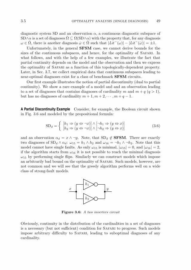
3.5 OPTIMALITY ANALYSIS (SINGLE DIAGNOSIS) 49
diagnostic system SD and an observation α, a continuous diagnostic subspace ofSD∧α is a set of diagnoses Ω ⊆ Ω(SD∧α) with the property that, for any diagnosisω ∈ Ω, there is another diagnosis ω ∈ Ω such that |Lit−(ω)| − |Lit−(ω)| = ±1.
Unfortunately, in the general SFSM case, we cannot derive bounds for thesizes of the continuous subspaces, and hence, for the optimality of Safari. Inwhat follows, and with the help of a few examples, we illustrate the fact thatpartial continuity depends on the model and the observation and then we expressthe optimality of Safari as a function of this topologically-dependent property.Later, in Sec. 3.7, we collect empirical data that continuous subspaces leading tonear-optimal diagnoses exist for a class of benchmark SFSM circuits.
Our first example illustrates the notion of partial discontinuity (dual to partialcontinuity). We show a rare example of a model and and an observation leadingto a set of diagnoses that contains diagnoses of cardinality m and m+ q (q > 1),but has no diagnoses of cardinality m+ 1,m+ 2, · · · ,m+ q − 1.
A Partial Discontinuity Example Consider, for example, the Boolean circuit shownin Fig. 3.6 and modeled by the propositional formula:
SDd =
[h1 ⇒ (y ⇔ ¬x)] ∧ [¬h1 ⇒ (y ⇔ x)][h2 ⇒ (y ⇔ ¬x)] ∧ [¬h2 ⇒ (y ⇔ x)]
(3.6)
and an observation αd = x ∧ ¬y. Note, that SDd 6∈ SFSM. There are exactlytwo diagnoses of SDd ∧ αd: ω15 = h1 ∧ h2 and ω16 = ¬h1 ∧ ¬h2. Note that thismodel cannot have single faults. As only ω15 is minimal, |ω15| = 0, and |ω16| = 2,if the algorithm starts from ω16 it is not possible to reach the minimal diagnosisω15 by performing single flips. Similarly we can construct models which imposean arbitrarily bad bound on the optimality of Safari. Such models, however, arenot common and we will see that the greedy algorithm performs well on a wideclass of strong-fault models.
h1
h2
x y
Figure 3.6: A two inverters circuit
Obviously, continuity in the distribution of the cardinalities in a set of diagnosesis a necessary (but not sufficient) condition for Safari to progress. Such modelsimpose arbitrary difficulty to Safari, leading to suboptimal diagnoses of anycardinality.
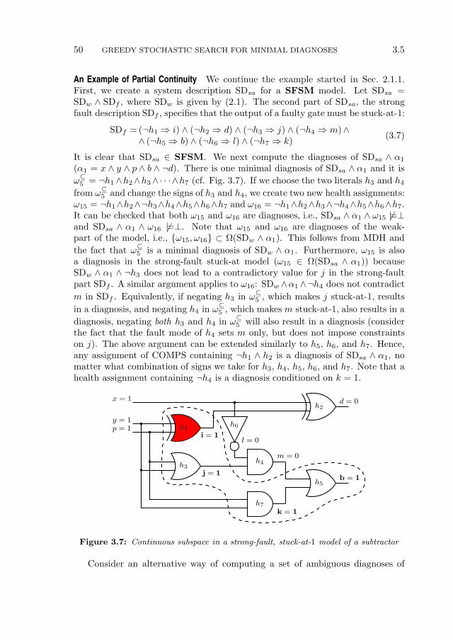
50 GREEDY STOCHASTIC SEARCH FOR MINIMAL DIAGNOSES 3.5
An Example of Partial Continuity We continue the example started in Sec. 2.1.1.First, we create a system description SDsa for a SFSM model. Let SDsa =SDw ∧ SDf , where SDw is given by (2.1). The second part of SDsa, the strongfault description SDf , specifies that the output of a faulty gate must be stuck-at-1:
SDf =(¬h1 ⇒ i) ∧ (¬h2 ⇒ d) ∧ (¬h3 ⇒ j) ∧ (¬h4 ⇒ m)∧∧ (¬h5 ⇒ b) ∧ (¬h6 ⇒ l) ∧ (¬h7 ⇒ k)
(3.7)
It is clear that SDsa ∈ SFSM. We next compute the diagnoses of SDsa ∧ α1
(α1 = x ∧ y ∧ p ∧ b ∧ ¬d). There is one minimal diagnosis of SDsa ∧ α1 and it is
ω⊆5 = ¬h1∧h2∧h3∧· · ·∧h7 (cf. Fig. 3.7). If we choose the two literals h3 and h4
from ω⊆5 and change the signs of h3 and h4, we create two new health assignments:
ω15 = ¬h1∧h2∧¬h3∧h4∧h5∧h6∧h7 and ω16 = ¬h1∧h2∧h3∧¬h4∧h5∧h6∧h7.It can be checked that both ω15 and ω16 are diagnoses, i.e., SDsa ∧ α1 ∧ ω15 6|=⊥and SDsa ∧ α1 ∧ ω16 6|=⊥. Note that ω15 and ω16 are diagnoses of the weak-part of the model, i.e., ω15, ω16 ⊂ Ω(SDw ∧ α1). This follows from MDH and
the fact that ω⊆5 is a minimal diagnosis of SDw ∧ α1. Furthermore, ω15 is also
a diagnosis in the strong-fault stuck-at model (ω15 ∈ Ω(SDsa ∧ α1)) becauseSDw ∧ α1 ∧ ¬h3 does not lead to a contradictory value for j in the strong-faultpart SDf . A similar argument applies to ω16: SDw ∧α1∧¬h4 does not contradict
m in SDf . Equivalently, if negating h3 in ω⊆5 , which makes j stuck-at-1, results
in a diagnosis, and negating h4 in ω⊆5 , which makes m stuck-at-1, also results in a
diagnosis, negating both h3 and h4 in ω⊆5 will also result in a diagnosis (consider
the fact that the fault mode of h4 sets m only, but does not impose constraintson j). The above argument can be extended similarly to h5, h6, and h7. Hence,any assignment of COMPS containing ¬h1 ∧ h2 is a diagnosis of SDsa ∧ α1, nomatter what combination of signs we take for h3, h4, h5, h6, and h7. Note that ahealth assignment containing ¬h4 is a diagnosis conditioned on k = 1.
h6
x = 1
y = 1p = 1
j = 1
d = 0
b = 1
h3h4
h5
h1
i = 1l = 0
k = 1
m = 0
h7
h2
Figure 3.7: Continuous subspace in a strong-fault, stuck-at-1 model of a subtractor
Consider an alternative way of computing a set of ambiguous diagnoses of
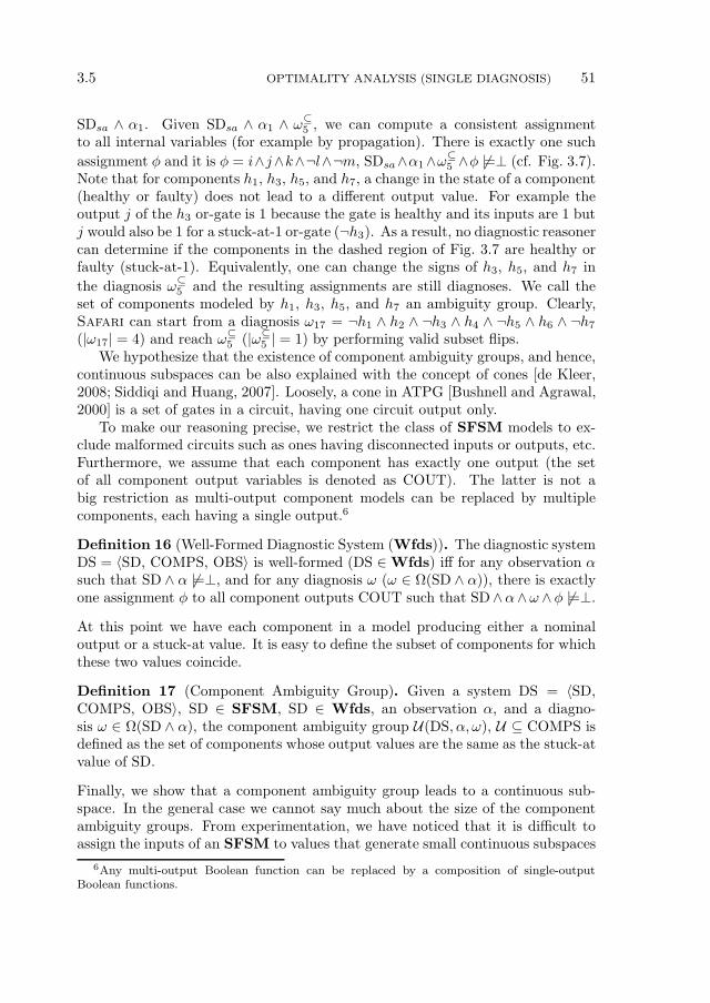
3.5 OPTIMALITY ANALYSIS (SINGLE DIAGNOSIS) 51
SDsa ∧ α1. Given SDsa ∧ α1 ∧ ω⊆5 , we can compute a consistent assignment
to all internal variables (for example by propagation). There is exactly one such
assignment φ and it is φ = i∧j∧k∧¬l∧¬m, SDsa∧α1∧ω⊆5 ∧φ 6|=⊥ (cf. Fig. 3.7).
Note that for components h1, h3, h5, and h7, a change in the state of a component(healthy or faulty) does not lead to a different output value. For example theoutput j of the h3 or-gate is 1 because the gate is healthy and its inputs are 1 butj would also be 1 for a stuck-at-1 or-gate (¬h3). As a result, no diagnostic reasonercan determine if the components in the dashed region of Fig. 3.7 are healthy orfaulty (stuck-at-1). Equivalently, one can change the signs of h3, h5, and h7 in
the diagnosis ω⊆5 and the resulting assignments are still diagnoses. We call the
set of components modeled by h1, h3, h5, and h7 an ambiguity group. Clearly,Safari can start from a diagnosis ω17 = ¬h1 ∧ h2 ∧ ¬h3 ∧ h4 ∧ ¬h5 ∧ h6 ∧ ¬h7
(|ω17| = 4) and reach ω⊆5 (|ω⊆
5 | = 1) by performing valid subset flips.We hypothesize that the existence of component ambiguity groups, and hence,
continuous subspaces can be also explained with the concept of cones [de Kleer,2008; Siddiqi and Huang, 2007]. Loosely, a cone in ATPG [Bushnell and Agrawal,2000] is a set of gates in a circuit, having one circuit output only.
To make our reasoning precise, we restrict the class of SFSM models to ex-clude malformed circuits such as ones having disconnected inputs or outputs, etc.Furthermore, we assume that each component has exactly one output (the setof all component output variables is denoted as COUT). The latter is not abig restriction as multi-output component models can be replaced by multiplecomponents, each having a single output.6
Definition 16 (Well-Formed Diagnostic System (Wfds)). The diagnostic systemDS = 〈SD, COMPS, OBS〉 is well-formed (DS ∈Wfds) iff for any observation αsuch that SD ∧ α 6|=⊥, and for any diagnosis ω (ω ∈ Ω(SD ∧ α)), there is exactlyone assignment φ to all component outputs COUT such that SD∧α∧ω ∧φ 6|=⊥.
At this point we have each component in a model producing either a nominaloutput or a stuck-at value. It is easy to define the subset of components for whichthese two values coincide.
Definition 17 (Component Ambiguity Group). Given a system DS = 〈SD,COMPS, OBS〉, SD ∈ SFSM, SD ∈ Wfds, an observation α, and a diagno-sis ω ∈ Ω(SD ∧ α), the component ambiguity group U(DS, α, ω), U ⊆ COMPS isdefined as the set of components whose output values are the same as the stuck-atvalue of SD.
Finally, we show that a component ambiguity group leads to a continuous sub-space. In the general case we cannot say much about the size of the componentambiguity groups. From experimentation, we have noticed that it is difficult toassign the inputs of an SFSM to values that generate small continuous subspaces
6Any multi-output Boolean function can be replaced by a composition of single-outputBoolean functions.

52 GREEDY STOCHASTIC SEARCH FOR MINIMAL DIAGNOSES 3.5
(either SD ∧ α |=⊥, or SD ∧ α leads to large component ambiguity groups). Ofcourse, it is possible to consider an adder, or a multiplier, for example, whoseinputs are all zeroes and whose gate models are all stuck-at-1 when faulty, butthe number of such inputs/circuit combinations is small.
Proposition 2. A diagnostic system SD, SD ∈ SFSM, SD ∈ Wfds, and anobservation α entail continuous diagnostic subspaces.
Proof. From Def. 16 and the fact that SD ∈ Wfds it follows that the outputvalues of a subset of the components have the same sign as the model’s stuck-at value. We denote this set as COMPS′, COMPS′ ⊆ COMPS. Any healthassignment ω that differs only in signs of components belonging to COMPS′ isalso a diagnosis. If the set of diagnoses of SD∧α contains all possible assignmentsto the assumables in COMPS′ then those diagnoses form a continuous space (cf.Def. 17).
To best illustrate Proposition 2, consider the or-gate modeled by h3 in Fig. 3.7.Its output is 1 either because the gate is healthy and one of the gate’s inputs is 1or because the gate is stuck-at-1. In this situation, it is not possible to determineif the component is healthy or faulty.
Clearly, |U(DS, α, ω)| is a lower bound for the progress of Safari in stuck-atmodels. It can be shown that if Safari starts from a diagnosis ω of maximumcardinality for the given subspace, Safari is guaranteed (for M = |COMPS|)to improve the cardinality of ω by at least |U(DS, α, ω)|. In practice, Safari
can proceed even further as the stuck-at ambiguity groups are only one factorof diagnostic uncertainty. A stuck-at component effectively “disconnects” inputsfrom outputs, hence gates from the fan-in region are not constrained. For instance,continuing our example, for ¬h5, all predecessors in the cone of ¬h5 (components¬h3, ¬h4, ¬h5, ¬h6, and ¬h7) constitute a continuous health subspace. Contraryto a component ambiguity group, this set is conditional on the health state ofanother component. A thorough study of stuck-at continuity is outside the scopeof this thesis but as we shall see in Sec. 3.7, continuous subspaces justify Safari
experiments on stuck-at models.
Performance Modeling with Stuck-At Models
To further study the optimality of Safari in strong-fault models, we first define acase in which the algorithm cannot improve a non-minimal diagnosis by changingthe sign of a faulty literal. Note that the existence of such cases is not a sufficientcondition for Safari to be suboptimal, as it is possible to reach a minimal diag-nosis by first changing the sign of some other faulty literal, thus “circumventing”the missing diagnosis.
From the preceding section we know that the number of “invalid flips” doesnot depend on k, i.e., it is determined by the observation vector and the fault
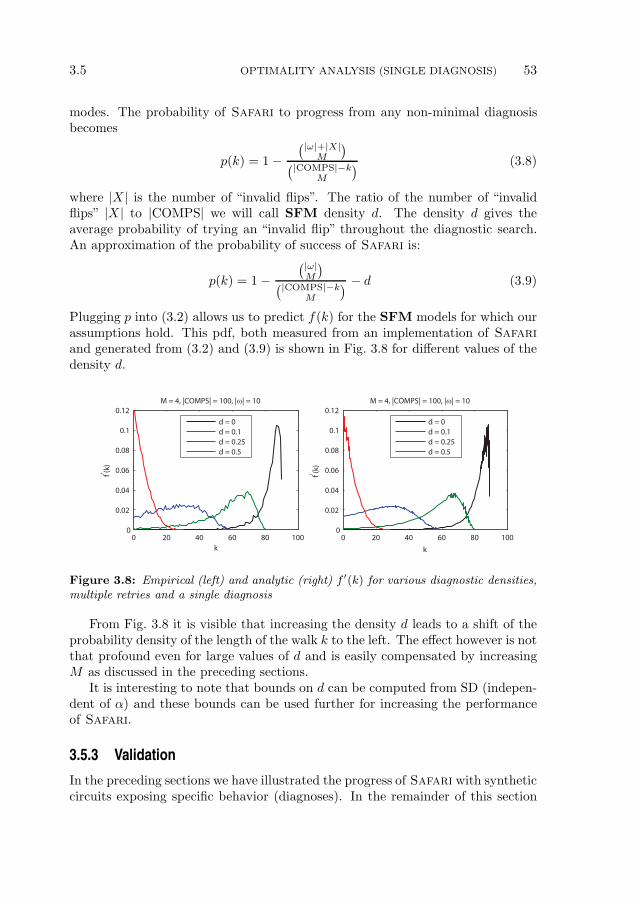
3.5 OPTIMALITY ANALYSIS (SINGLE DIAGNOSIS) 53
modes. The probability of Safari to progress from any non-minimal diagnosisbecomes
p(k) = 1−(|ω|+|X|
M
)(|COMPS|−k
M
) (3.8)
where |X | is the number of “invalid flips”. The ratio of the number of “invalidflips” |X | to |COMPS| we will call SFM density d. The density d gives theaverage probability of trying an “invalid flip” throughout the diagnostic search.An approximation of the probability of success of Safari is:
p(k) = 1−(|ω|M
)(|COMPS|−k
M
) − d (3.9)
Plugging p into (3.2) allows us to predict f(k) for the SFM models for which ourassumptions hold. This pdf, both measured from an implementation of Safari
and generated from (3.2) and (3.9) is shown in Fig. 3.8 for different values of thedensity d.
0 20 40 60 80 1000
0.02
0.04
0.06
0.08
0.1
0.12
k
f’ (k)
M = 4, |COMPS| = 100, |ω| = 10
d = 0d = 0.1
d = 0.25d = 0.5
0 20 40 60 80 1000
0.02
0.04
0.06
0.08
0.1
0.12M = 4, |COMPS| = 100, |ω| = 10
k
f’ (k)
d = 0d = 0.1
d = 0.25d = 0.5
Figure 3.8: Empirical (left) and analytic (right) f ′(k) for various diagnostic densities,multiple retries and a single diagnosis
From Fig. 3.8 it is visible that increasing the density d leads to a shift of theprobability density of the length of the walk k to the left. The effect however is notthat profound even for large values of d and is easily compensated by increasingM as discussed in the preceding sections.
It is interesting to note that bounds on d can be computed from SD (indepen-dent of α) and these bounds can be used further for increasing the performanceof Safari.
3.5.3 Validation
In the preceding sections we have illustrated the progress of Safari with syntheticcircuits exposing specific behavior (diagnoses). In the remainder of this section

54 GREEDY STOCHASTIC SEARCH FOR MINIMAL DIAGNOSES 3.5
we will plot the pdf of the greedy search on one of the small benchmark circuits(for more information on the 74181 model cf. Sec. 3.7).
The progress of Safari with a weak-fault model of the 74181 circuit is shownin Fig. 3.9. We have chosen a difficult observation leading to a minimal diagnosisof cardinality 7 (left) and an easy observation leading to a single fault diagno-sis (right). Both plots show that the probability mass shifts to the right whenincreasing M and the effect is more profound for the smaller cardinality.
0 10 20 30 40 50 600
0.1
0.2
0.3
0.4
0.574181, |ω| = 7
k
f’ (k)
30 40 50 60 700
0.1
0.2
0.3
0.4
0.574181, |ω| = 1
k
f’ (k)
M = 1
M = 2
M = 3
M = 4
M = 1
M = 2
M = 3
M = 4
Figure 3.9: Empirical f ′(k) for a weak-fault model of the 74181 circuit with observa-tions leading to two different minimal-cardinality diagnoses and various M
The effect of the stuck-at-0 and stuck-at-1 fault modes (SFM) on the probabilityof success of Safari is shown in Fig. 3.10.
20 30 40 50 600
0.05
0.1
0.15
0.274181, |ω| = 6, S-A-0
k
f’ (k)
10 20 30 40 50 600
0.05
0.1
0.15
0.274181, |ω| = 6, S-A-1
k
f’ (k)
M = 1
M = 2
M = 3
M = 4
M = 1
M = 2
M = 3
M = 4
Figure 3.10: Empirical f ′(k) for stuck-at-0 and stuck-at-1 strong-fault models of the74181 circuit with various M
Obviously, in this case the effect of increasing M is smaller, although still de-pending on the difficulty of the observation vector. Last, even for small valuesof M , the absolute probability of Safari finding a minimal diagnosis is sizeable,allowing the use of Safari as a practical anytime algorithm which always re-

3.6 OPTIMALITY ANALYSIS (MULTIPLE DIAGNOSES) 55
turns a diagnosis, the optimality of which depends on the time allocated to itscomputation.
3.6 Optimality Analysis (Multiple Diagnoses)
The preceding section described the process of computing one diagnosis withSafari (N = 1). In this section we discuss the use of Safari in computing (orcounting) all minimal-cardinality diagnoses (N > 1). For the rest of the sectionwe will assume that Safari is configured with M = |COMPS|.
Consider a system description SD (SD ∈WFM) and an observation α. Thenumber of minimal diagnoses |Ω⊆(SD∧α)| can be exponential in |COMPS|. Fur-thermore, in practice, diagnosticians are interested in sampling from the set ofminimal-cardinality diagnoses Ω≤(SD∧α) (recall that Ω≤(SD∧α) ⊆ Ω⊆(SD∧α))as the minimal-cardinality diagnoses cover a significant part of the a posterioridiagnosis probability space [de Kleer, 1990]. In what follows, we will see thatSafari is very well suited for that task.
Theorem 3. The probability of Safari configured with M = |COMPS| comput-ing a minimal diagnosis of cardinality |ω| in a system with |COMPS| componentvariables approaches |COMPS|−|ω| for |COMPS|/|ω| → ∞.
Proof (Sketch). Assume a minimal diagnosis of cardinality |ω| exists. From Propo-sition 1 it follows that Safari configured with M = |COMPS| is guaranteed tocompute minimal diagnoses. Starting from the “all faulty” assignment, consider astep k in “improving” the diagnosis cardinality. If state k contains more than onediagnosis, then at state k+1, Safari will either (1) flip a literal belonging to thisdiagnosis (note that a literal may belong to more than one diagnosis) and sub-sequently prevent Safari of reaching this diagnosis or (2) flip a literal belongingto a diagnosis which has already been invalidated (i.e., one or more of its literalshave been flipped at an earlier step).
The probability that a solution of cardinality |ω| “survives” a flip at iterationk (i.e., is not invalidated) is:
p (k) = 1− |ω||COMPS| − k =
|COMPS| − |ω| − k|COMPS| − k (3.10)
Similarly to our basic model (Sec. 3.5.1), the probability that a diagnosis ω “sur-vives” until it is returned by the algorithm:
f(|COMPS| − |ω| − 1) =
|COMPS|−|ω|−1∏
i=0
p(i) = (3.11)
=
|COMPS|−|ω|−1∏
i=0
|COMPS| − |ω| − i|COMPS| − i (3.12)
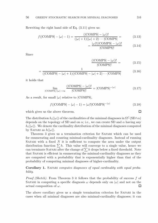
56 GREEDY STOCHASTIC SEARCH FOR MINIMAL DIAGNOSES 3.6
Rewriting the right hand side of Eq. (3.11) gives us:
f(|COMPS| − |ω| − 1) =(|COMPS| − |ω|)!
(|ω|+ 1)(|ω|+ 2) · · · |COMPS| = (3.13)
=|ω|!(|COMPS| − |ω|)!
|COMPS|! (3.14)
Since
(|COMPS| − |ω|)!|COMPS|! = (3.15)
=1
(|COMPS| − |ω|+ 1)(|COMPS| − |ω|+ 2) · · · |COMPS| (3.16)
it holds that
lim|COMPS|/|ω|→∞
(|COMPS| − |ω|)!|COMPS|! = |COMPS|−|ω| (3.17)
As a result, for small |ω| relative to |COMPS|,
f(|COMPS| − |ω| − 1) = |ω|!|COMPS|−|ω| (3.18)
which gives us the above theorem.
The distribution hi(|ω|) of the cardinalities of the minimal diagnoses in Ω⊆(SD∧α)depends on the topology of SD and on α; i.e., we can create SD and α having anyhi(|ω|). We denote the cardinality distribution of the minimal diagnoses computedby Safari as h(|ω|).
Theorem 3 gives us a termination criterion for Safari which can be usedfor enumerating and counting minimal-cardinality diagnoses. Instead of runningSafari with a fixed N it is sufficient to compute the area under the outputdistribution function
∑h. This value will converge to a single value, hence we
can terminate Safari after the change of∑h drops below a fixed threshold. Note
that Safari is efficient in enumerating the minimal-cardinality diagnoses as theyare computed with a probability that is exponentially higher than that of theprobability of computing minimal diagnoses of higher-cardinality.
Corollary 1. Safari computes diagnoses of equal cardinality with equal proba-bility.
Proof (Sketch). From Theorem 3 it follows that the probability of success f ofSafari in computing a specific diagnosis ω depends only on |ω| and not on theactual composition of ω.
The above corollary gives us a simple termination criterion for Safari in thecases when all minimal diagnoses are also minimal-cardinality diagnoses; it can

3.6 OPTIMALITY ANALYSIS (MULTIPLE DIAGNOSES) 57
be proven that in this case all minimal-cardinality diagnoses are computed withthe same probability.
We will see that, given an input cardinality distribution hi(|ω|), Safari pro-duces an output distribution h(|ω|) that is highly skewed to the right due toTheorem 3. To facilitate the study of how Safari transforms hi(|ω|) into h(|ω|)we will use a Monte Carlo simulation of Safari. The advantage is that the MonteCarlo simulation is much simpler for analysing the run-time behavior of Safari
than studying the algorithm itself.
Algorithm 2 Monte Carlo simulation of Safari.
1: function SafariSimulate(Ω⊆, N) returns a cardinality distribution
inputs: Ω⊆, a set of minimal diagnosesN , integer, number of tries
local variables: hi, vector, cardinality distributionsh, vector, cardinality distributionb, vector, fault distribution,n, integer, current runi, integerc, integer
2: hi ← CardinalityDistribution(Ω⊆)3: for n← 1, 2, . . . , N do
4: for c← 1, 2, . . . , |hi| do
5: b[c]← c · hi[c]6: end for
7: for i← 1, 2, . . . , |Ω⊆| do
8: c← DiscreteInverseRandomValue
(b∑b
)
9: b[c]← b[c]− c10: end for
11: h[c]← h[c] + 112: end for
13: return h14: end function
Algorithm 2 simulates which diagnoses from the input set of minimal diagnoses Ωare “reached” by Safari in N tries. The auxiliary subroutine CardinalityDis-
tribution computes the input distribution hi by iterating over all diagnoses inΩ⊆. We store the input cardinality distribution hi and the resulting cardinalitydistribution h in vectors (note the vector sums in lines 7 and 8 and the divisionof a vector by scalar in line 8).
The outermost loop of Alg. 2 (lines 3 – 12) simulates the N runs of Safari.This is done by computing and updating an auxiliary vector b, which contains thedistribution of the component variables in Ω⊆ according to the cardinalities of
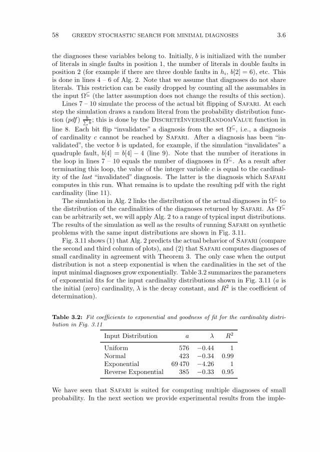
58 GREEDY STOCHASTIC SEARCH FOR MINIMAL DIAGNOSES 3.6
the diagnoses these variables belong to. Initially, b is initialized with the numberof literals in single faults in position 1, the number of literals in double faults inposition 2 (for example if there are three double faults in hi, b[2] = 6), etc. Thisis done in lines 4 – 6 of Alg. 2. Note that we assume that diagnoses do not shareliterals. This restriction can be easily dropped by counting all the assumables inthe input Ω⊆ (the latter assumption does not change the results of this section).
Lines 7 – 10 simulate the process of the actual bit flipping of Safari. At eachstep the simulation draws a random literal from the probability distribution func-tion (pdf) b∑
b ; this is done by the DiscreteInverseRandomValue function in
line 8. Each bit flip “invalidates” a diagnosis from the set Ω⊆, i.e., a diagnosisof cardinality c cannot be reached by Safari. After a diagnosis has been “in-validated”, the vector b is updated, for example, if the simulation “invalidates” aquadruple fault, b[4] = b[4] − 4 (line 9). Note that the number of iterations inthe loop in lines 7 – 10 equals the number of diagnoses in Ω⊆. As a result afterterminating this loop, the value of the integer variable c is equal to the cardinal-ity of the last “invalidated” diagnosis. The latter is the diagnosis which Safari
computes in this run. What remains is to update the resulting pdf with the rightcardinality (line 11).
The simulation in Alg. 2 links the distribution of the actual diagnoses in Ω⊆ tothe distribution of the cardinalities of the diagnoses returned by Safari. As Ω⊆
can be arbitrarily set, we will apply Alg. 2 to a range of typical input distributions.The results of the simulation as well as the results of running Safari on syntheticproblems with the same input distributions are shown in Fig. 3.11.
Fig. 3.11 shows (1) that Alg. 2 predicts the actual behavior of Safari (comparethe second and third column of plots), and (2) that Safari computes diagnoses ofsmall cardinality in agreement with Theorem 3. The only case when the outputdistribution is not a steep exponential is when the cardinalities in the set of theinput minimal diagnoses grow exponentially. Table 3.2 summarizes the parametersof exponential fits for the input cardinality distributions shown in Fig. 3.11 (a isthe initial (zero) cardinality, λ is the decay constant, and R2 is the coefficient ofdetermination).
Table 3.2: Fit coefficients to exponential and goodness of fit for the cardinality distri-bution in Fig. 3.11
Input Distribution a λ R2
Uniform 576 −0.44 1Normal 423 −0.34 0.99Exponential 69 470 −4.26 1Reverse Exponential 385 −0.33 0.95
We have seen that Safari is suited for computing multiple diagnoses of smallprobability. In the next section we provide experimental results from the imple-
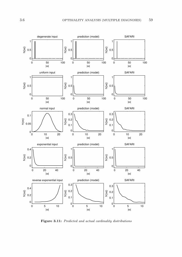
3.6 OPTIMALITY ANALYSIS (MULTIPLE DIAGNOSES) 59
0 50 100
0
0.5
1
degenerate input
|ω|
h(|
ω|)
0 50 100
0
0.5
1
prediction (model)
|ω|h
(|ω
|)0 50 100
0
0.5
1
SAFARI
|ω|
h(|
ω|)
0 50 100
0
0.5
1
SAFARI
|ω|
h(|
ω|)
0 50 100
0
0.5
1
prediction (model)
|ω|
h(|
ω|)
0 50 100
0
0.5
1
uniform input
|ω|
h(|
ω|)
0 10 20
0
0.1
0.2
0.3
SAFARI
|ω|
h(|
ω|)
0 10 20
0
0.1
0.2
0.3
prediction (model)
|ω|
h(|
ω|)
0 10 200
0.05
0.1
normal input
|ω|
h(|
ω|)
0 20 40
0
0.5
1
SAFARI
|ω|
h(|
ω|)
0 20 40
0
0.5
1
prediction (model)
|ω|
h(|
ω|)
0 20 40
0
0.2
0.4
exponential input
|ω|
h(|
ω|)
0 5 10
0
0.2
0.4
reverse exponential input
|ω|
h(|
ω|)
0 5 100
0.1
0.2
0.3
prediction (model)
|ω|
h(|
ω|)
0 5 100
0.1
0.2
0.3
SAFARI
|ω|
h(|
ω|)
Figure 3.11: Predicted and actual cardinality distributions
60 GREEDY STOCHASTIC SEARCH FOR MINIMAL DIAGNOSES 3.7
mentation of Safari and related algorithms.
3.7 Experimental Results
This section discusses empirical results measured from an implementation of Sa-
fari. In order to compare the optimality and performance of Safari to variousdiagnostic algorithms, we have performed more than a million diagnosis compu-tations on 64 dual-CPU nodes belonging to a cluster. Each node contains two 2.4GHz AMD Opteron DP 250 processors and 4 Gb of RAM.
The default configuration of Safari (when not stated otherwise) was M = 8and N = 4; that is, Safari is configured for a maximum number of 8 retriesbefore giving up the climb, and a total of 4 attempts. To provide more preciseaverage run-time optimality and performance data, all stochastic algorithms (e.g.,ones based on SLS Max-SAT and Safari) have been repeatedly run 10 times oneach model and observation vector.
3.7.1 Implementation Notes and Test Set Description
We have implemented Safari in approximately 1 000 lines of C code (excludingthe LTMS, interface, and DPLL code) and it is a part of the Lydia package.7
We have performed our experiments on the benchmark circuits described inSec. 2.4. In order to provide both weak- and strong-fault cases, we have translatedeach circuit to a weak, stuck-at-0 (S-A-0), and stuck-at-1 (S-A-1) model. In thestuck-at models, the output of each faulty gate is assumed to be the same constant(cf. Def. 14).
The performance of diagnostic algorithms depends to various degrees on theobservation vectors (algorithm designers strive to produce algorithms, the perfor-mance of which is not dependent on the observation vectors). Hence, we haveperformed our experimentation with a number of different observations for eachmodel. We have implemented an algorithm (Alg. 3) that generates observationsleading to diagnoses of different minimal-cardinality, varying from 1 to nearly themaximum for the respective circuits (for the 74XXX models it is the maximum).The experiments omit nominal scenarios as they are trivial from the viewpoint ofMBD.
Algorithm 3 uses a number of auxiliary functions. RandomInputs (line 3)assigns uniformly distributed random values to each input in IN (note that for thegeneration of observation vectors we partition the observable variables OBS intoinputs IN and outputs OUT and use the input/output information which comeswith the original 74XXX/ISCAS85 circuits for simulation). Given the“all healthy”health assignment and the diagnostic system, ComputeNominalOutputs (line
7Lydia, Safari, and the diagnostic benchmark are freely available for download athttp://fdir.org/lydia/.
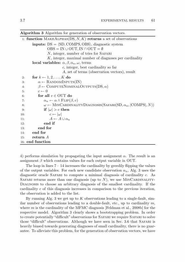
3.7 EXPERIMENTAL RESULTS 61
Algorithm 3 Algorithm for generation of observation vectors.
1: function MakeAlphas(DS, N,K) returns a set of observations
inputs: DS = 〈SD,COMPS,OBS〉, diagnostic systemOBS = IN ∪OUT, IN ∩OUT = ∅N , integer, number of tries for Safari
K, integer, maximal number of diagnoses per cardinalitylocal variables: α, β, αn, ω, terms
c, integer, best cardinality so farA, set of terms (observation vectors), result
2: for k ← 1, 2, . . . ,K do
3: α← RandomInputs(IN)4: β ← ComputeNominalOutputs(DS, α)5: c← 06: for all v ∈ OUT do
7: αn ← α ∧Flip(β, v)8: ω ←MinCardinalityDiagnosis(Safari(SD, αn, |COMPS|, N))9: if |ω| > c then
10: c← |ω|11: A← A ∪ αn
12: end if
13: end for
14: end for
15: return A16: end function
4) performs simulation by propagating the input assignment α. The result is anassignment β which contains values for each output variable in OUT.
The loop in lines 7 – 14 increases the cardinality by greedily flipping the valuesof the output variables. For each new candidate observation αn, Alg. 3 uses thediagnostic oracle Safari to compute a minimal diagnosis of cardinality c. AsSafari returns more than one diagnosis (up to N), we use MinCardinality-
Diagnosis to choose an arbitrary diagnosis of the smallest cardinality. If thecardinality c of this diagnosis increases in comparison to the previous iteration,the observation is added to the list.
By running Alg. 3 we get up to K observations leading to a single-fault, sim-ilar number of observations leading to a double-fault, etc., up to cardinality m,where m is the cardinality of the MFMC diagnosis [Feldman et al., 2008b] for therespective model. Algorithm 3 clearly shows a bootstrapping problem. In orderto create potentially“difficult”observations for Safari we require Safari to solvethose “difficult” observations. Although we have seen in Sec. 3.6 that Safari isheavily biased towards generating diagnoses of small cardinality, there is no guar-antee. To alleviate this problem, for the generation of observation vectors, we have
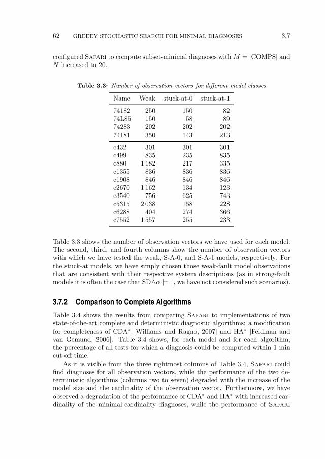
62 GREEDY STOCHASTIC SEARCH FOR MINIMAL DIAGNOSES 3.7
configured Safari to compute subset-minimal diagnoses with M = |COMPS| andN increased to 20.
Table 3.3: Number of observation vectors for different model classes
Name Weak stuck-at-0 stuck-at-1
74182 250 150 8274L85 150 58 8974283 202 202 20274181 350 143 213
c432 301 301 301c499 835 235 835c880 1 182 217 335c1355 836 836 836c1908 846 846 846c2670 1 162 134 123c3540 756 625 743c5315 2 038 158 228c6288 404 274 366c7552 1 557 255 233
Table 3.3 shows the number of observation vectors we have used for each model.The second, third, and fourth columns show the number of observation vectorswith which we have tested the weak, S-A-0, and S-A-1 models, respectively. Forthe stuck-at models, we have simply chosen those weak-fault model observationsthat are consistent with their respective system descriptions (as in strong-faultmodels it is often the case that SD∧α |=⊥, we have not considered such scenarios).
3.7.2 Comparison to Complete Algorithms
Table 3.4 shows the results from comparing Safari to implementations of twostate-of-the-art complete and deterministic diagnostic algorithms: a modificationfor completeness of CDA∗ [Williams and Ragno, 2007] and HA∗ [Feldman andvan Gemund, 2006]. Table 3.4 shows, for each model and for each algorithm,the percentage of all tests for which a diagnosis could be computed within 1 mincut-off time.
As it is visible from the three rightmost columns of Table 3.4, Safari couldfind diagnoses for all observation vectors, while the performance of the two de-terministic algorithms (columns two to seven) degraded with the increase of themodel size and the cardinality of the observation vector. Furthermore, we haveobserved a degradation of the performance of CDA∗ and HA∗ with increased car-dinality of the minimal-cardinality diagnoses, while the performance of Safari

3.7 EXPERIMENTAL RESULTS 63
Table 3.4: Comparison of CDA∗, HA∗, and Safari [% of tests solved]
CDA∗ HA∗ Safari
Name Weak S-A-0 S-A-1 Weak S-A-0 S-A-1 Weak S-A-0 S-A-1
74182 100 100 100 100 100 100 100 100 10074L85 100 100 100 100 100 100 100 100 10074283 100 100 100 100 100 100 100 100 10074181 79.1 98.6 97.7 100 100 100 100 100 100
c432 74.1 75.4 73.1 71.1 94.7 69.1 100 100 100c499 29 45.5 27.7 24.1 77.9 25.9 100 100 100c880 11.6 44.7 32.2 12.4 62.2 41.5 100 100 100c1355 3.8 4.7 5.4 10.8 10.6 12.2 100 100 100c1908 0 0 0 6.1 6 6.5 100 100 100c2670 0 0 0 5 64.2 44.7 100 100 100c3540 0 0 0 1.1 3.8 2.2 100 100 100c5315 0 0 0 1.1 8.2 5.7 100 100 100c6288 0 0 0 3.5 5.1 3.3 100 100 100c7552 0 0 0 3.9 7.8 12 100 100 100
remained unaffected.
In what follows we compare Safari to two DXC’09 [Feldman et al., 2010]algorithms: NGDE [de Kleer, 2009] and RODON [Karin et al., 2006]. This com-parison has been performed in the DXC’09 experimental framework. For moreinformation on the conditions under which we have evaluated the performance ofNGDE, RODON, and Safari, cf. [Feldman et al., 2010].
NGDE is an Allegro Common Lisp implementation of the classic GDE. NGDEuses a minimum-cardinality candidate generator to construct diagnoses from con-flicts. For ADAPT-Lite it uses interval constraints.
RODON [Karin et al., 2006] is based on the principles of GDE as described byde Kleer and Williams [1987] and the G+DE [Heller and Struss, 2001]. RODONuses contradictions (conflicts) between the simulated and the observed behaviorto generate hypotheses about possible causes for the observed behavior. If themodel contains failure modes in addition to the nominal behavior, these can beused to verify the hypotheses, which speeds up the diagnostic process and improvethe results.
Table 3.5 shows the Mutl, Mcpu, and Mmem metrics (cf. Sec. 2.5). It can beseen that Safari has achieved significantly better Mcpu and Mmem than NGDE[de Kleer, 2009] and RODON [Karin et al., 2006]. Mutl of Safari is slightly worsedue to smaller number of diagnostic candidates computed by this DA. Safari andRODON showed similar results in the utility metrics.
Table 3.6 shows the Msru, Mdru, and Merr metrics. We can see that Mdru does
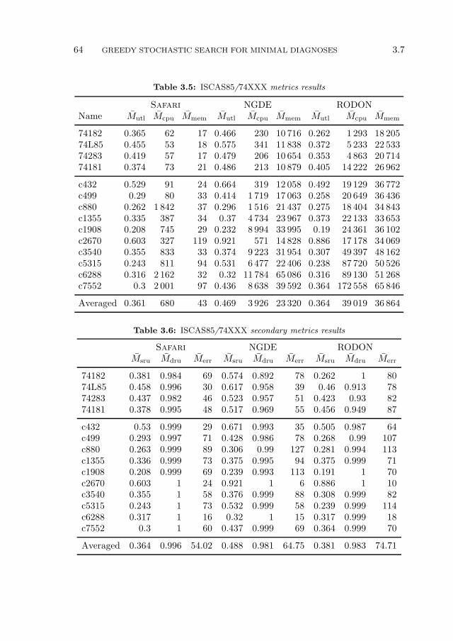
64 GREEDY STOCHASTIC SEARCH FOR MINIMAL DIAGNOSES 3.7
Table 3.5: ISCAS85/74XXX metrics results
Safari NGDE RODONName Mutl Mcpu Mmem Mutl Mcpu Mmem Mutl Mcpu Mmem
74182 0.365 62 17 0.466 230 10 716 0.262 1 293 18 20574L85 0.455 53 18 0.575 341 11 838 0.372 5 233 22 53374283 0.419 57 17 0.479 206 10 654 0.353 4 863 20 71474181 0.374 73 21 0.486 213 10 879 0.405 14 222 26 962
c432 0.529 91 24 0.664 319 12 058 0.492 19 129 36 772c499 0.29 80 33 0.414 1 719 17 063 0.258 20 649 36 436c880 0.262 1 842 37 0.296 1 516 21 437 0.275 18 404 34 843c1355 0.335 387 34 0.37 4 734 23 967 0.373 22 133 33 653c1908 0.208 745 29 0.232 8 994 33 995 0.19 24 361 36 102c2670 0.603 327 119 0.921 571 14 828 0.886 17 178 34 069c3540 0.355 833 33 0.374 9 223 31 954 0.307 49 397 48 162c5315 0.243 811 94 0.531 6 477 22 406 0.238 87 720 50 526c6288 0.316 2 162 32 0.32 11 784 65 086 0.316 89 130 51 268c7552 0.3 2 001 97 0.436 8 638 39 592 0.364 172 558 65 846
Averaged 0.361 680 43 0.469 3 926 23 320 0.364 39 019 36 864
Table 3.6: ISCAS85/74XXX secondary metrics results
Safari NGDE RODONMsru Mdru Merr Msru Mdru Merr Msru Mdru Merr
74182 0.381 0.984 69 0.574 0.892 78 0.262 1 8074L85 0.458 0.996 30 0.617 0.958 39 0.46 0.913 7874283 0.437 0.982 46 0.523 0.957 51 0.423 0.93 8274181 0.378 0.995 48 0.517 0.969 55 0.456 0.949 87
c432 0.53 0.999 29 0.671 0.993 35 0.505 0.987 64c499 0.293 0.997 71 0.428 0.986 78 0.268 0.99 107c880 0.263 0.999 89 0.306 0.99 127 0.281 0.994 113c1355 0.336 0.999 73 0.375 0.995 94 0.375 0.999 71c1908 0.208 0.999 69 0.239 0.993 113 0.191 1 70c2670 0.603 1 24 0.921 1 6 0.886 1 10c3540 0.355 1 58 0.376 0.999 88 0.308 0.999 82c5315 0.243 1 73 0.532 0.999 58 0.239 0.999 114c6288 0.317 1 16 0.32 1 15 0.317 0.999 18c7552 0.3 1 60 0.437 0.999 69 0.364 0.999 70
Averaged 0.364 0.996 54.02 0.488 0.981 64.75 0.381 0.983 74.71
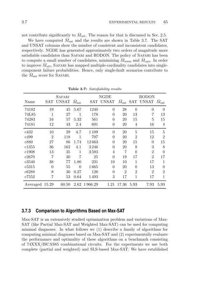
3.7 EXPERIMENTAL RESULTS 65
not contribute significantly to Mutl. The reason for that is discussed in Sec. 2.5.
We have computed Msat and the results are shown in Table 3.7. The SATand UNSAT columns show the number of consistent and inconsistent candidates,respectively. NGDE has generated approximately two orders of magnitude moresatisfiable candidates than Safari and RODON. The policy of Safari has beento compute a small number of candidates, minimizing Mmem and Mcpu. In orderto improve Mutl, Safari has mapped multiple-cardinality candidates into single-component failure probabilities. Hence, only single-fault scenarios contribute tothe Msat score for Safari.
Table 3.7: Satisfiability results
Safari NGDE RODONName SAT UNSAT Msat SAT UNSAT Msat SAT UNSAT Msat
74182 19 45 5.67 1240 0 28 0 0 074L85 1 27 1 178 0 20 13 7 1374283 34 57 5.32 561 0 20 15 5 1574181 12 43 2.4 691 0 20 4 16 4
c432 10 29 4.7 1 109 0 20 5 15 5c499 2 118 1 707 0 20 2 12 2c880 27 86 1.74 12 663 0 20 15 0 15c1355 36 162 4.1 3 246 0 20 8 3 8c1908 13 35 1 3 593 4 7 0 2 0c2670 7 30 7 25 0 19 17 2 17c3540 38 77 1.86 231 10 10 1 17 1c5315 0 55 0 1 665 0 20 0 13 0c6288 8 30 0.27 126 0 2 2 2 2c7552 7 53 0.64 1 493 3 17 1 17 1
Averaged 15.29 60.50 2.62 1 966.29 1.21 17.36 5.93 7.93 5.93
3.7.3 Comparison to Algorithms Based on Max-SAT
Max-SAT is an extensively studied optimization problem and variations of Max-SAT (like Partial Max-SAT and Weighted Max-SAT) can be used for computingminimal diagnoses. In what follows we (1) describe a family of algorithms forcomputing minimal diagnoses based on Max-SAT and (2) experimentally evaluatethe performance and optimality of these algorithms on a benchmark consistingof 74XXX/ISCAS85 combinational circuits. For the experiments we use bothcomplete (partial and weighted) and SLS-based Max-SAT. We have established
66 GREEDY STOCHASTIC SEARCH FOR MINIMAL DIAGNOSES 3.7
that the performance of complete Max-SAT and the optimality of SLS-basedMax-SAT degrade when increasing the circuit size or the cardinality of the faults.
Given a formula Φ in CNF, a Max-SAT [Hoos and Stutzle, 2004] solution isa variable assignment that maximizes the number of satisfied clauses in Φ (inmost cases of interest Φ is unsatisfiable, otherwise any variable assignment whichsatisfies Φ is also a Max-SAT solution). In partial Max-SAT some of the clauses inΦ are designated as hard, the others are“soft”. A solution to the partial Max-SATproblem should satisfy all “hard” clauses and maximize the number of satisfied“soft” clauses. Similarly, in weighted Max-SAT a weight is assigned to each clausein Φ and a solution maximizes the sum of the weights of the satisfied clauses.
In this section we (1) show how to use Max-SAT for computing minimal di-agnoses, (2) study the performance of a family of Max-SAT-based diagnosticalgorithms, and (3) empirically compare the performance and optimality of theMax-SAT-based algorithms to Safari. The results show that, although diagnosisbased on Max-SAT performs better than other algorithms for computing min-imal diagnosis, specialized stochastic solvers like Safari outperform Max-SATby at least an order-of-magnitude for the class of diagnostic problems we haveconsidered. This is not surprising, as specialized MBD algorithms exploit specificproperties of the search space, as we will describe.
A Max-SAT-Based MBD Algorithm
We have used the approach of Sang et al. [2007] for encoding Most ProbableExplanation (MPE) as Max-SAT. Computing MPE is identical to computing amost-probable diagnosis in a more general framework. Algorithm 4 computesdiagnoses by calling a Max-SAT oracle.
Note that the diagnostic problems we solve in this chapter can be translatedto multiple optimization problems which can be solved with SAT-based methods[Giunchiglia and Maratea, 2006]. The Maximum Satisfiable Subset (MSS) prob-lem, for example, is dual to the Minimal Unsatisfiable Subset problem [Bailey andStuckey, 2005] and the two can be solved with Max-SAT and Min-UNSAT solvers,respectively [Liffiton and Sakallah, 2005]. From those, we have found preference inthe research community towards Max-SAT, and for practical reasons we thereforecompare Safari to Max-SAT.
Algorithm 4 adds a unit clause with weight 1 for each assumable (line 6).The weight of each input clause is set to a value greater than the number of allassumables (line 3). The loop in lines 8 – 11 computes a diagnosis with a call toMax-SAT (the auxiliary subroutine HealthLiterals computes a diagnosis froma Max-SAT assignment by filtering the health literals) and if a diagnosis exists, itis added to the result (line 10). Finally, the negation of each diagnosis is added tothe original set of clauses (line 9) to prevent subsequent computation of the samediagnosis. Note that the negation of a term is conveniently a clause.
Depending on the implementation of the Max-SAT call in line 8 of Alg. 4we have a family of Max-SAT algorithms for diagnosis: (1) if Max-SAT is a

3.7 EXPERIMENTAL RESULTS 67
Algorithm 4 Weighted Max-SAT based diagnosis algorithm.
1: function MaxSATDiagnose(DS, α) returns a set of diagnoses
inputs: DS = 〈SD,COMPS,OBS〉, diagnostic systemα, term, observation
local variables: W , set of clauses; Ω, set of diagnosesω, diagnosis term; c, clause; h, variable
2: for all c ∈ Clauses(SD) do
3: W ←W ∪ 〈∞, c〉4: end for
5: for all h ∈ COMPS do
6: W ←W ∪ 〈1, c〉7: end for
8: while ω ← HealthLiterals(Max-SAT(W )) do
9: W ←W ∪ 〈∞,¬ω〉10: Ω← Ω ∪ ω11: end while
12: return Ω13: end function
partial Max-SAT solver, Alg. 4 computes diagnoses ordered by cardinality; (2)if Max-SAT is a weighted Max-SAT solver, Alg. 4 computes diagnoses orderedby probability; and (3) if Max-SAT is based on SLS, not every iteration of themain loop yields a diagnosis. We have run extensive experiments with all threeMax-SAT variants, which we describe in the following sub-sections.
Experimental Results with Complete Max-SAT
We next show the performance of Alg. 4 with two partial Max-SAT algorithms(partial and weighted Max-SAT algorithms are always complete).Table 3.8 shows performance results of the partial Max-SAT solver W-MaxSatz
[Argelich et al., 2007] and the weighted MiniMaxSat [Heras et al., 2008]. Notethat the performance of W-MaxSatz in weighted mode is slightly worse thanwhen solving the respective partial formulae. Both solvers are state-of-the-art andhave been submitted to the Second Max-SAT Evaluation 2007.8 The performanceof the complete Max-SAT solvers degrades with increasing circuit size and thecardinality of the injected faults. The results of those algorithms are comparableto, or slightly better, than the performance of CDA∗ and HA∗. For comparison,Safari solves all test instances.
Our findings are consistent with the ones of Giunchiglia and Maratea [2006].In their paper, Giunchiglia and Maratea [2006] report ISCAS85 times similar tothe ones measured with state-of-the-art Max-SAT solvers where no solver com-
8http://www.maxsat07.udl.es/
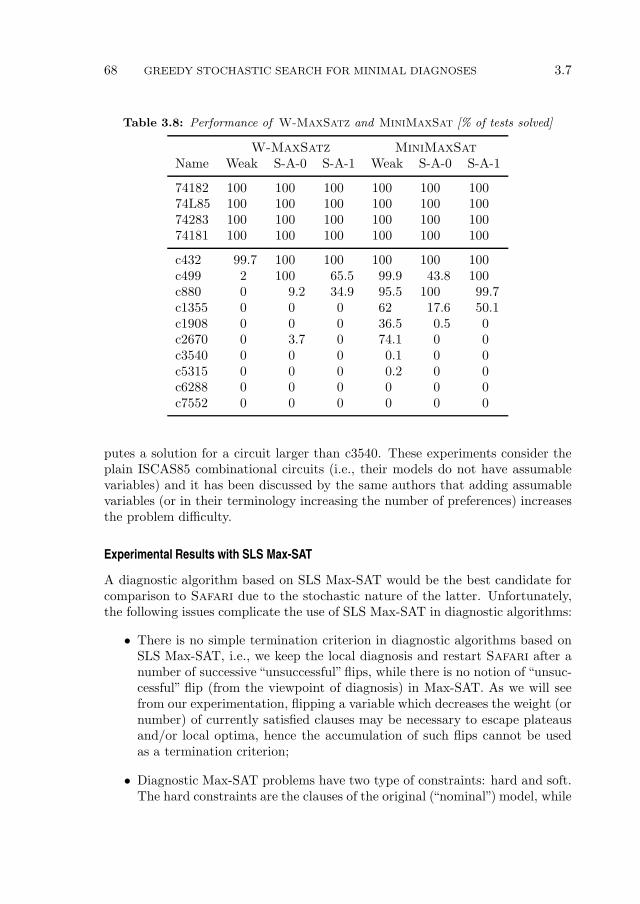
68 GREEDY STOCHASTIC SEARCH FOR MINIMAL DIAGNOSES 3.7
Table 3.8: Performance of W-MaxSatz and MiniMaxSat [% of tests solved]
W-MaxSatz MiniMaxSat
Name Weak S-A-0 S-A-1 Weak S-A-0 S-A-1
74182 100 100 100 100 100 10074L85 100 100 100 100 100 10074283 100 100 100 100 100 10074181 100 100 100 100 100 100
c432 99.7 100 100 100 100 100c499 2 100 65.5 99.9 43.8 100c880 0 9.2 34.9 95.5 100 99.7c1355 0 0 0 62 17.6 50.1c1908 0 0 0 36.5 0.5 0c2670 0 3.7 0 74.1 0 0c3540 0 0 0 0.1 0 0c5315 0 0 0 0.2 0 0c6288 0 0 0 0 0 0c7552 0 0 0 0 0 0
putes a solution for a circuit larger than c3540. These experiments consider theplain ISCAS85 combinational circuits (i.e., their models do not have assumablevariables) and it has been discussed by the same authors that adding assumablevariables (or in their terminology increasing the number of preferences) increasesthe problem difficulty.
Experimental Results with SLS Max-SAT
A diagnostic algorithm based on SLS Max-SAT would be the best candidate forcomparison to Safari due to the stochastic nature of the latter. Unfortunately,the following issues complicate the use of SLS Max-SAT in diagnostic algorithms:
• There is no simple termination criterion in diagnostic algorithms based onSLS Max-SAT, i.e., we keep the local diagnosis and restart Safari after anumber of successive “unsuccessful” flips, while there is no notion of “unsuc-cessful” flip (from the viewpoint of diagnosis) in Max-SAT. As we will seefrom our experimentation, flipping a variable which decreases the weight (ornumber) of currently satisfied clauses may be necessary to escape plateausand/or local optima, hence the accumulation of such flips cannot be usedas a termination criterion;
• Diagnostic Max-SAT problems have two type of constraints: hard and soft.The hard constraints are the clauses of the original (“nominal”) model, while

3.7 EXPERIMENTAL RESULTS 69
the soft constraints are the unit clauses received from the assumable vari-ables. An SLS Max-SAT algorithm does not distinguish between those hardand soft clauses; if such an algorithm guaranteed the satisfaction of thehard-constraints it would be classified as hybrid and not stochastic.
The two reasons above prevent us from using a diagnostic reasoner based on SLSMax-SAT in practical applications. Despite that, we have conducted extensiveexperimentation with UBCSAT [Tompkins and Hoos, 2005] in order to evaluatethe potential of SLS Max-SAT in MBD.
To overcome the termination problems with SLS Max-SAT, for the followingexperiments, we have chosen observations leading to known single faults. Foreach WFM we have chosen 50 observations. We have configured the SLS Max-SAT search to terminate after 100 000 variable flips and we have modified Alg. 4 toterminate after 10 calls to Max-SAT. The resulting optimality of algorithms basedon SLS Max-SAT in computing single fault diagnoses is shown in Table 3.9. Wehave run experiments with all algorithms or algorithm variants implemented bythe UBCSAT suite, covering the algorithms RGSAT, Schoening, CDRW, throughGSAT.
The data in Table 3.9 show best cases. From each of the 500 Max-SAT invoca-tions per algorithm/circuit (50 single faults, 10 runs per experiment) we have (1)ignored all results which do not satisfy all hard constraints, (2) recorded the bestdiagnostic cardinality achieved in the hill climbing (recall that these are single-faults hence the best result is 1) and (3) recorded the number of steps (bit flips)in which this best diagnostic cardinality was achieved (the number of bit-flips aregiven in parentheses below the optimality number in Table 3.9).
Table 3.9 shows the generally poor performance of SLS Max-SAT algorithms.In most of the cases the algorithm could either never satisfy all hard-constraints orachieved increasingly worse cardinality with the growth of the circuit. Exceptionsare the two variants of SAPS [Hutter et al., 2002] and we attribute this relativelygood optimality of SAPS to its mechanism for assigning and updating weights toclauses based on the clause length. Recall that in our diagnostic problems clausesof assumable literals have unit weights while hard-constraints have weights greaterthan the number of assumable literals. Despite that, in the best case for c7552,SAPS needed 77 264 bit flips to find the optimal single-fault diagnosis. In com-parison Safari performed 11 bit flips, and although an LTMS/SAT consistencycheck of Safari is strictly more expensive than the consistency checking of SLSMax-SAT (the former is worst-case NP-hard while the latter is in P), Safari iscomputationally more efficient on average.
Figure 3.12 illustrates the progress of two SLS Max-SAT invocations. TheConflict-Directed Random Walk (CDRW) [Papadimitriou, 1991] starts with arandom variable assignment and flips the most profitable (for increasing the satis-fied weight) variable. This often leads to violated hard-constraints (due to flippingof non-assumable variables), and the restarts which are needed for escaping thosesituations lead to the relatively noisy ascent of CDRW. Other SLS Max-SAT al-
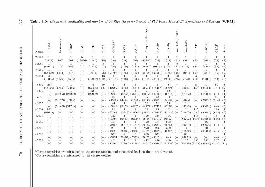
70
GR
EE
DY
ST
OC
HA
ST
ICSE
AR
CH
FO
RM
INIM
AL
DIA
GN
OSE
S3.7 Table 3.9: Diagnostic cardinality and number of bit-flips (in parentheses) of SLS-based Max-SAT algorithms and Safari (WFM)
Name RG
SAT
Sch
oenin
g
CD
RW
URW
IRoT
S
RoT
S
G2W
SAT
SA
PS
a
SA
PS
b
Adapti
ve
Novelty+
Novelty+
Novelty
Walk
SAT
/TA
BU
Walk
SAT
HSAT
GW
SAT
GSAT
Safari
74182 1 1 1 9 1 1 1 1 1 1 1 1 1 1 1 1 1 1(4331) (163) (501) (29896) (1265) (19) (40) (40) (76) (42260) (28) (56) (21) (37) (26) (186) (38) (2)
74L85 1 1 1 − 1 3 1 1 1 1 1 1 5 1 1 1 1 1(65623) (276) (353) (−) (7236) (27) (39) (199) (143) (80782) (9815) (1267) (47) (116) (34) (629) (34) (4)
74283 1 1 1 − 1 1 1 1 1 1 1 1 4 1 1 1 1 1(63429) (1134) (573) (−) (3644) (26) (21806) (166) (112) (25003) (31900) (435) (35) (1034) (29) (187) (32) (2)
74181 4 1 1 − 1 13 1 1 1 1 1 1 10 1 3 1 3 1(48395) (4525) (6542) (−) (49967) (1498) (1814) (146) (453) (1045) (81883) (2060) (75) (2123) (67) (1139) (54) (3)
c432 28 1 1 − 4 36 4 1 1 7 1 8 − 1 13 1 16 1(43176) (1866) (7452) (−) (82496) (101) (10262) (806) (564) (20211) (75488) (16393) (−) (905) (133) (24164) (167) (2)
c499 − 1 1 − 29 − 6 1 1 7 5 13 − 1 − 1 − 1(−) (24203) (95242) (−) (99999) (−) (98683) (42534) (66519) (2112) (87589) (49516) (−) (47102) (−) (45465) (−) (1)
c880 − 1 1 − − − 26 1 1 35 23 30 − 1 − 1 46 1(−) (36269) (8388) (−) (−) (−) (9561) (4244) (1551) (5680) (80926) (34989) (−) (9825) (−) (27026) (304) (5)
c1355 − 2 1 − − − 44 1 1 52 51 53 − 1 − 1 − 1(−) (93549) (34235) (−) (−) (−) (83944) (9670) (4975) (84777) (67454) (85365) (−) (34786) (−) (93656) (−) (5)
c1908 240 − − − − − 91 1 1 94 98 101 − 1 125 1 139 1(68649) (−) (−) (−) (−) (−) (97567) (95942) (19664) (5142) (79442) (43541) (−) (50660) (654) (94695) (643) (6)
c2670 − − − − − − 122 1 1 126 135 144 − 1 173 1 177 1(−) (−) (−) (−) (−) (−) (93799) (9547) (6635) (19000) (67042) (6532) (−) (83292) (1008) (85581) (976) (5)
c3540 − − − − − − 167 1 1 170 177 203 − 1 − 16 − 1(−) (−) (−) (−) (−) (−) (79188) (16376) (17776) (88052) (68342) (68663) (−) (99209) (−) (93639) (−) (9)
c5315 − − − − − − 261 1 1 270 275 329 − 14 − 70 − 1(−) (−) (−) (−) (−) (−) (78093) (79438) (48388) (64079) (96973) (48497) (−) (98557) (−) (89462) (−) (9)
c6288 − − − − − − 329 4 8 360 372 − − 58 − − − 1(−) (−) (−) (−) (−) (−) (23191) (79807) (73752) (36373) (91636) (−) (−) (94673) (−) (−) (−) (3)
c7552 − − − − − − 403 1 1 412 440 449 − 115 492 181 507 1(−) (−) (−) (−) (−) (−) (12905) (77264) (42284) (39046) (90485) (32732) (−) (90449) (2543) (99340) (2552) (11)
aClause penalties are initialized to the clause weights and smoothed back to their initial values.bClause penalties are initialized to the clause weights.
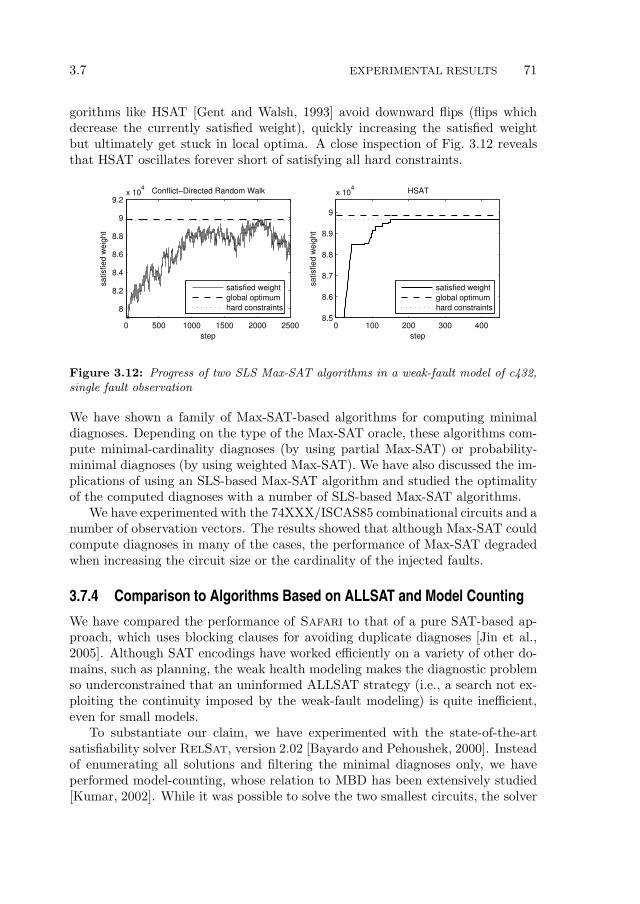
3.7 EXPERIMENTAL RESULTS 71
gorithms like HSAT [Gent and Walsh, 1993] avoid downward flips (flips whichdecrease the currently satisfied weight), quickly increasing the satisfied weightbut ultimately get stuck in local optima. A close inspection of Fig. 3.12 revealsthat HSAT oscillates forever short of satisfying all hard constraints.
0 500 1000 1500 2000 2500
8
8.2
8.4
8.6
8.8
9
9.2x 10
4
step
satisfied w
eig
ht
Conflict−Directed Random Walk
0 100 200 300 4008.5
8.6
8.7
8.8
8.9
9
x 104 HSAT
step
satisfied w
eig
ht
satisfied weight
global optimum
hard constraints
satisfied weight
global optimum
hard constraints
Figure 3.12: Progress of two SLS Max-SAT algorithms in a weak-fault model of c432,single fault observation
We have shown a family of Max-SAT-based algorithms for computing minimaldiagnoses. Depending on the type of the Max-SAT oracle, these algorithms com-pute minimal-cardinality diagnoses (by using partial Max-SAT) or probability-minimal diagnoses (by using weighted Max-SAT). We have also discussed the im-plications of using an SLS-based Max-SAT algorithm and studied the optimalityof the computed diagnoses with a number of SLS-based Max-SAT algorithms.
We have experimented with the 74XXX/ISCAS85 combinational circuits and anumber of observation vectors. The results showed that although Max-SAT couldcompute diagnoses in many of the cases, the performance of Max-SAT degradedwhen increasing the circuit size or the cardinality of the injected faults.
3.7.4 Comparison to Algorithms Based on ALLSAT and Model Counting
We have compared the performance of Safari to that of a pure SAT-based ap-proach, which uses blocking clauses for avoiding duplicate diagnoses [Jin et al.,2005]. Although SAT encodings have worked efficiently on a variety of other do-mains, such as planning, the weak health modeling makes the diagnostic problemso underconstrained that an uninformed ALLSAT strategy (i.e., a search not ex-ploiting the continuity imposed by the weak-fault modeling) is quite inefficient,even for small models.
To substantiate our claim, we have experimented with the state-of-the-artsatisfiability solver RelSat, version 2.02 [Bayardo and Pehoushek, 2000]. Insteadof enumerating all solutions and filtering the minimal diagnoses only, we haveperformed model-counting, whose relation to MBD has been extensively studied[Kumar, 2002]. While it was possible to solve the two smallest circuits, the solver
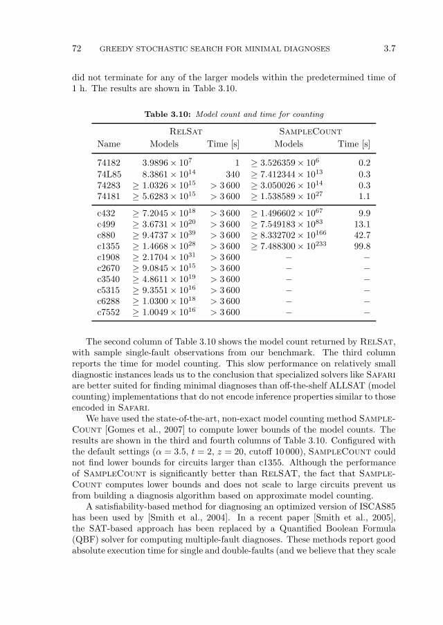
72 GREEDY STOCHASTIC SEARCH FOR MINIMAL DIAGNOSES 3.7
did not terminate for any of the larger models within the predetermined time of1 h. The results are shown in Table 3.10.
Table 3.10: Model count and time for counting
RelSat SampleCount
Name Models Time [s] Models Time [s]
74182 3.9896× 10⁷ 1 ≥ 3.526359× 10⁶ 0.2
74L85 8.3861× 10¹⁴ 340 ≥ 7.412344× 10¹³ 0.374283 ≥ 1.0326× 10¹⁵ > 3 600 ≥ 3.050026× 10¹⁴ 0.374181 ≥ 5.6283× 10¹⁵ > 3 600 ≥ 1.538589× 1027 1.1
c432 ≥ 7.2045× 10¹⁸ > 3 600 ≥ 1.496602× 1067 9.9c499 ≥ 3.6731× 10²⁰ > 3 600 ≥ 7.549183× 1083 13.1c880 ≥ 9.4737× 1039 > 3 600 ≥ 8.332702× 10166 42.7c1355 ≥ 1.4668× 1028 > 3 600 ≥ 7.488300× 10233 99.8c1908 ≥ 2.1704× 1031 > 3 600 − −c2670 ≥ 9.0845× 10¹⁵ > 3 600 − −c3540 ≥ 4.8611× 10¹⁹ > 3 600 − −c5315 ≥ 9.3551× 10¹⁶ > 3 600 − −c6288 ≥ 1.0300× 10¹⁸ > 3 600 − −c7552 ≥ 1.0049× 10¹⁶ > 3 600 − −
The second column of Table 3.10 shows the model count returned by RelSat,with sample single-fault observations from our benchmark. The third columnreports the time for model counting. This slow performance on relatively smalldiagnostic instances leads us to the conclusion that specialized solvers like Safari
are better suited for finding minimal diagnoses than off-the-shelf ALLSAT (modelcounting) implementations that do not encode inference properties similar to thoseencoded in Safari.
We have used the state-of-the-art, non-exact model counting method Sample-
Count [Gomes et al., 2007] to compute lower bounds of the model counts. Theresults are shown in the third and fourth columns of Table 3.10. Configured withthe default settings (α = 3.5, t = 2, z = 20, cutoff 10 000), SampleCount couldnot find lower bounds for circuits larger than c1355. Although the performanceof SampleCount is significantly better than RelSAT, the fact that Sample-
Count computes lower bounds and does not scale to large circuits prevent usfrom building a diagnosis algorithm based on approximate model counting.
A satisfiability-based method for diagnosing an optimized version of ISCAS85has been used by [Smith et al., 2004]. In a recent paper [Smith et al., 2005],the SAT-based approach has been replaced by a Quantified Boolean Formula(QBF) solver for computing multiple-fault diagnoses. These methods report goodabsolute execution time for single and double-faults (and we believe that they scale
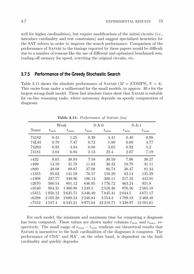
3.7 EXPERIMENTAL RESULTS 73
well for higher cardinalities), but require modifications of the initial circuits (i.e.,introduce cardinality and test constraints) and suggest specialized heuristics forthe SAT solvers in order to improve the search performance. Comparison of theperformance of Safari to the timings reported by these papers would be difficultdue to a number of reasons like the use of different and optimized benchmark sets,trading-off memory for speed, rewriting the original circuits, etc.
3.7.5 Performance of the Greedy Stochastic Search
Table 3.11 shows the absolute performance of Safari (M = |COMPS|, N = 4).This varies from under a millisecond for the small models, to approx. 30 s for thelargest strong-fault model. These fast absolute times show that Safari is suitablefor on-line reasoning tasks, where autonomy depends on speedy computation ofdiagnosis.
Table 3.11: Performance of Safari [ms]
Weak S-A-0 S-A-1Name tmin tmax tmin tmax tmin tmax
74182 0.41 1.25 0.39 4.41 0.40 0.9874L85 0.78 7.47 0.72 1.89 0.69 4.7774283 0.92 4.84 0.88 3.65 0.92 5.274181 2.04 6.94 2.13 22.4 2.07 7.19
c432 8.65 38.94 7.58 30.59 7.96 38.27c499 14.19 31.78 11.03 30.32 10.79 31.11c880 48.08 88.87 37.08 80.74 38.47 81.34c1355 95.03 141.59 76.57 150.29 83.14 135.29c1908 237.77 349.96 196.13 300.11 217.32 442.91c2670 500.54 801.12 646.95 1 776.72 463.24 931.8c3540 984.31 1 300.98 1 248.5 2 516.46 976.56 2 565.18c5315 1 950.12 2 635.71 3 346.49 7 845.41 2 034.5 4 671.17c6288 2 105.28 2 688.34 2 246.84 3 554.4 1 799.18 2 469.48c7552 4 557.4 6 545.21 9 975.04 32 210.71 5 338.97 12 101.61
For each model, the minimum and maximum time for computing a diagnosishas been computed. These values are shown under columns tmin and tmax , re-spectively. The small range of tmax − tmin confirms our theoretical results thatSafari is insensitive to the fault cardinalities of the diagnoses it computes. Theperformance of CDA∗ and HA∗, on the other hand, is dependent on the faultcardinality and quickly degrades.
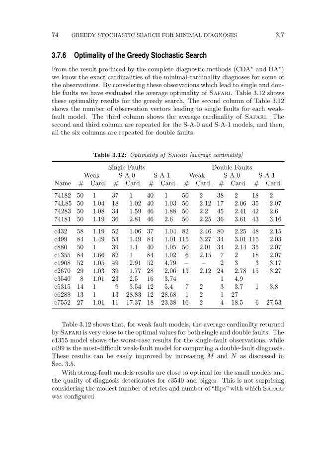
74 GREEDY STOCHASTIC SEARCH FOR MINIMAL DIAGNOSES 3.7
3.7.6 Optimality of the Greedy Stochastic Search
From the result produced by the complete diagnostic methods (CDA∗ and HA∗)we know the exact cardinalities of the minimal-cardinality diagnoses for some ofthe observations. By considering these observations which lead to single and dou-ble faults we have evaluated the average optimality of Safari. Table 3.12 showsthese optimality results for the greedy search. The second column of Table 3.12shows the number of observation vectors leading to single faults for each weak-fault model. The third column shows the average cardinality of Safari. Thesecond and third column are repeated for the S-A-0 and S-A-1 models, and then,all the six columns are repeated for double faults.
Table 3.12: Optimality of Safari [average cardinality]
Single Faults Double FaultsWeak S-A-0 S-A-1 Weak S-A-0 S-A-1
Name # Card. # Card. # Card. # Card. # Card. # Card.
74182 50 1 37 1 40 1 50 2 38 2 18 274L85 50 1.04 18 1.02 40 1.03 50 2.12 17 2.06 35 2.0774283 50 1.08 34 1.59 46 1.88 50 2.2 45 2.41 42 2.674181 50 1.19 36 2.81 46 2.6 50 2.25 36 3.61 43 3.16
c432 58 1.19 52 1.06 37 1.04 82 2.46 80 2.25 48 2.15c499 84 1.49 53 1.49 84 1.01 115 3.27 34 3.01 115 2.03c880 50 1 39 1.1 40 1.05 50 2.01 34 2.14 35 2.07c1355 84 1.66 82 1 84 1.02 6 2.15 7 2 18 2.07c1908 52 1.05 49 2.91 52 4.79 − − 2 3 3 3.17c2670 29 1.03 39 1.77 28 2.06 13 2.12 24 2.78 15 3.27c3540 8 1.01 23 2.5 16 3.74 − − 1 4.9 − −c5315 14 1 9 3.54 12 5.4 7 2 3 3.7 1 3.8c6288 13 1 13 28.83 12 28.68 1 2 1 27 − −c7552 27 1.01 11 17.37 18 23.38 16 2 4 18.5 6 27.53
Table 3.12 shows that, for weak fault models, the average cardinality returnedby Safari is very close to the optimal values for both single and double faults. Thec1355 model shows the worst-case results for the single-fault observations, whilec499 is the most-difficult weak-fault model for computing a double-fault diagnosis.These results can be easily improved by increasing M and N as discussed inSec. 3.5.
With strong-fault models results are close to optimal for the small models andthe quality of diagnosis deteriorates for c3540 and bigger. This is not surprisingconsidering the modest number of retries and number of “flips”with which Safari
was configured.
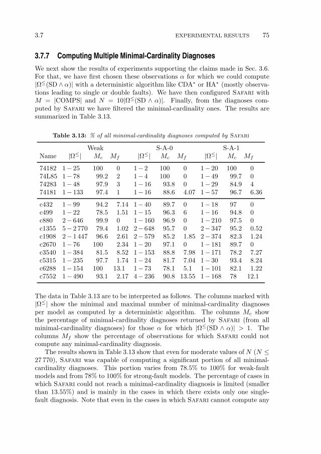
3.7 EXPERIMENTAL RESULTS 75
3.7.7 Computing Multiple Minimal-Cardinality Diagnoses
We next show the results of experiments supporting the claims made in Sec. 3.6.For that, we have first chosen these observations α for which we could compute|Ω≤(SD ∧ α)| with a deterministic algorithm like CDA∗ or HA∗ (mostly observa-tions leading to single or double faults). We have then configured Safari withM = |COMPS| and N = 10|Ω≤(SD ∧ α)|. Finally, from the diagnoses com-puted by Safari we have filtered the minimal-cardinality ones. The results aresummarized in Table 3.13.
Table 3.13: % of all minimal-cardinality diagnoses computed by Safari
Weak S-A-0 S-A-1Name |Ω≤| Mc Mf |Ω≤| Mc Mf |Ω≤| Mc Mf
74182 1− 25 100 0 1− 2 100 0 1− 20 100 074L85 1− 78 99.2 2 1− 4 100 0 1− 49 99.7 074283 1− 48 97.9 3 1− 16 93.8 0 1− 29 84.9 474181 1− 133 97.4 1 1− 16 88.6 4.07 1− 57 96.7 6.36
c432 1− 99 94.2 7.14 1− 40 89.7 0 1− 18 97 0c499 1− 22 78.5 1.51 1− 15 96.3 6 1− 16 94.8 0c880 2− 646 99.9 0 1− 160 96.9 0 1− 210 97.5 0c1355 5− 2 770 79.4 1.02 2− 648 95.7 0 2− 347 95.2 0.52c1908 2− 1 447 96.6 2.61 2− 579 85.2 1.85 2− 374 82.3 1.24c2670 1− 76 100 2.34 1− 20 97.1 0 1− 181 89.7 0c3540 1− 384 81.5 8.52 1− 153 88.8 7.98 1− 171 78.2 7.27c5315 1− 235 97.7 1.74 1− 24 81.7 7.04 1− 30 93.4 8.24c6288 1− 154 100 13.1 1− 73 78.1 5.1 1− 101 82.1 1.22c7552 1− 490 93.1 2.17 4− 236 90.8 13.55 1− 168 78 12.1
The data in Table 3.13 are to be interpreted as follows. The columns marked with|Ω≤| show the minimal and maximal number of minimal-cardinality diagnosesper model as computed by a deterministic algorithm. The columns Mc showthe percentage of minimal-cardinality diagnoses returned by Safari (from allminimal-cardinality diagnoses) for those α for which |Ω≤(SD ∧ α)| > 1. Thecolumns Mf show the percentage of observations for which Safari could notcompute any minimal-cardinality diagnosis.
The results shown in Table 3.13 show that even for moderate values of N (N ≤27 770), Safari was capable of computing a significant portion of all minimal-cardinality diagnoses. This portion varies from 78.5% to 100% for weak-faultmodels and from 78% to 100% for strong-fault models. The percentage of cases inwhich Safari could not reach a minimal-cardinality diagnosis is limited (smallerthan 13.55%) and is mainly in the cases in which there exists only one single-fault diagnosis. Note that even in the cases in which Safari cannot compute any
76 GREEDY STOCHASTIC SEARCH FOR MINIMAL DIAGNOSES 3.8
minimal-cardinality diagnoses, the result of Safari can be useful. For example, asubset-minimal diagnosis of small cardinality differing in one or two literals only,still brings useful diagnostic information (a discussion on diagnostic metrics isbeyond the scope of this chapter).
3.7.8 Experimentation Summary
We have applied Safari to a suite of benchmark combinatorial circuits encodedusing weak fault models and stuck-at strong fault models, and shown significantperformance improvements for multiple-fault diagnoses, compared to two state-of-the-art deterministic algorithms, CDA∗ and HA∗. Our results indicate thatSafari shows at least an order-of-magnitude speedup over CDA∗ and HA∗ formultiple-fault diagnoses. Moreover, whereas the search complexity for the de-terministic algorithms tested increases exponentially with fault cardinality, thesearch complexity for this stochastic algorithm appears to be independent of faultcardinality.
We have compared the performance of Safari to that of an algorithm based onMax-SAT and Safari shows at least an order-of-magnitude speedup in computingdiagnoses. We have compared the optimality of Safari to that of an algorithmbased on SLS Max-SAT and Safari consistently computes diagnoses of smallercardinality whereas the SLS Max-SAT diagnostic algorithm often fails to computeany diagnoses.
3.8 Summary
We have described a greedy stochastic algorithm for computing diagnoses within amodel-based diagnosis framework. We have shown that subset-minimal diagnosescan be computed optimally in weak fault models and in an important subset ofstrong fault models, and that almost all minimal-cardinality diagnoses can becomputed for more general fault models.
We argue that Safari can be of broad practical significance, as it can computea significant fraction of minimal-cardinality diagnoses for systems too large orcomplex to be diagnosed by existing deterministic algorithms.
In future work, we plan to experiment on models with a combination of weakand strong failure-mode descriptions. We also plan on experimenting with a widervariety of stochastic methods, such as simulated annealing and genetic search,using a larger set of benchmark models. Last, we plan to apply our algorithms toa wider class of abduction and constraint optimization problems.
Chapter 4Computing Worst-Case Diagnostic
Scenarios
Model-Based Diagnosis (MBD) typically focuses on diagnoses, minimal undersome minimality criterion, e.g., the minimal-cardinality set of faulty componentsthat explain an observation α. However, for different α there may be minimal-car-dinality diagnoses of differing cardinalities, and several applications (such as testpattern generation and benchmark model analysis) need to identify the α leadingto the max-cardinality diagnosis amongst them. We denote this problem as aMax-Fault Min-Cardinality (MFMC) problem. This chapter considers the gener-ation of observations that lead to MFMC diagnoses. We present a near-optimal,stochastic algorithm, called Miranda (Max-fault mIn-caRdinAlity observatioNDeduction Algorithm), that computes MFMC observations. Compared to opti-mal, deterministic approaches such as ATPG, the algorithm has very low cost,allowing us to generate observations corresponding to high-cardinality faults.
4.1 Introduction
The problem of computing minimal-cardinality diagnoses, given an observationand a system description, is central to Model-Based Diagnosis [de Kleer and Wil-liams, 1987]. In this chapter we consider the “inverse” problem of computing anobservation that simultaneously isolates k faulty components. These observa-tions are useful in system testing and benchmarking of multiple-fault diagnostictechniques. Computing observations (in particular inputs) that distinguish a sin-gle failing component (k = 1) is studied by Automatic Test Pattern Generation(ATPG) and dates back to the D-algorithm [Roth, 1966]. The goal of ATPG isto compute a sequence of test vectors that can detect every possible single faultin a device. Single-fault ATPG has been extended to finding observation vec-
77
78 COMPUTING WORST-CASE DIAGNOSTIC SCENARIOS 4.2
tors leading to double faults [Hughes, 1988] and to multiple faults [Kubiak andFuchs, 1991]. These approaches have several drawbacks, including: (1) they donot determine the maximum possible value of k (2) they suffer from very highcomputational complexity, and (3) they severely limit the class of system abstrac-tions by imposing various model restrictions.
Few papers have proposed algorithms computing observation vectors that dis-tinguish the maximum number of failing components in a system [Abramovici,1981]. The GuidedProbe algorithm in the latter paper relies on probing toachieve the maximal fault resolution for a fixed test T . The author of this algo-rithm has a different goal, i.e., achieving maximal resolution by minimizing thenumber of probes, and proposes essentially a sequential algorithm. This is verydifferent from MBD approaches, which try to solve the multiple-fault problemwith only one observation.
To the best of our knowledge, we are the first to formally state the problem andsignificance of finding MFMC observations, and then to define an algorithm thatis able to approximate such a computationally difficult problem. Our methodis based on a greedy stochastic search algorithm, called Miranda (Max-faultmIn-caRdinAlity observatioN Deduction Algorithm), and uses an MBD oraclefor computing minimal-cardinality diagnoses. The algorithm is greedy in thatit monotonically exploits part of the problem search space. The performance isdetermined by the efficiency of the underlying MBD engine; i.e., it is efficient witha fast (usually incomplete) procedure for computing minimal-diagnoses.
One advantage of Miranda over related k-fault ATPG algorithms is that ituncovers the maximum value of k. Furthermore, it does not impose any limitationson the model (e.g., it neither requires no stuck-at modes nor assumes unlimitedobservability). This makes our approach applicable not only to system testingbut also to MBD benchmarking and to a wider range of Model-Based Reasoning(MBR) problems, such as optimal sensor placement [Console et al., 2000], activetesting, etc. In this chapter the MFMC algorithm is applied to MBD benchmark-ing [Provan and Wang, 2007], but it can be applied to compute a set of MFMCtest vectors covering all components in a system.
We have evaluated the performance of Miranda using the ISCAS85 bench-mark extended with 4 smaller circuits from the 74XXX family. For the 74XXXcircuits we have been able to exactly compute all MFMC observation vectors.Since deterministic MBD algorithms cannot compute the high fault-cardinalitiesassociated with MFMC vectors for the ISCAS85 circuits, we have used a stochasticMBD oracle [Feldman et al., 2008c].
4.2 A Range of MBD Problems
We continue with presenting a number of problems for computing observationvectors.
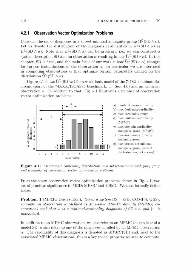
4.2 A RANGE OF MBD PROBLEMS 79
4.2.1 Observation Vector Optimization Problems
Consider the set of diagnoses in a subset-minimal ambiguity group Ω⊆(SD ∧ α).Let us denote the distribution of the diagnosis cardinalities in Ω⊆(SD ∧ α) as
Ω⊆(SD ∧ α). Note that Ω⊆(SD ∧ α) can be arbitrary, i.e., we can construct a
system description SD and an observation α resulting in any Ω⊆(SD∧α). In this
chapter, SD is fixed, and the main focus of our work is how Ω⊆(SD ∧ α) changesfor various instantiations of the observation α. In particular we are interestedin computing observations α that optimize certain parameters defined on thedistribution Ω⊆(SD ∧ α).
Figure 4.1 shows Ω⊆(SD∧α) for a weak-fault model of the 74182 combinatorialcircuit (part of the 74XXX/ISCAS85 benchmark, cf. Sec. 4.6) and an arbitraryobservation α. In addition to that, Fig. 4.1 illustrates a number of observationvector optimization problems.
0
1
2
3
4
5
6
7
#ofsu
bse
t-m
inim
al
dia
gnose
s
1 2 3 4 5 6 7 8 9 10 11 12
cardinality
a
e f
b
c
d
max-size subset-minimal
ambiguity group
max-size max-cardinality
ambiguity group (MSMC)
max-size min-cardinality
(MFMC)
max-fault min-cardinality
max-cardinality-range
max-fault max-cardinality
min-fault max-cardinalitya)
b)
c)
d)
e)
f)
g)
ambiguity group (area of
the histogram, not shown)
Figure 4.1: An example cardinality distribution in a subset-minimal ambiguity groupand a number of observation vector optimization problems
From the seven observation vector optimization problems shown in Fig. 4.1, twoare of practical significance to MBD: MFMC and MSMC. We next formally definethose.
Problem 1 (MFMC Observation). Given a system DS = 〈SD, COMPS, OBS〉,compute an observation α (defined as Max-Fault Min-Cardinality (MFMC) ob-servation) such that ω is a minimal-cardinality diagnosis of SD ∧ α and |ω| ismaximized.
In addition to an MFMC observation, we also refer to an MFMC diagnosis ω of amodel SD, which refers to any of the diagnoses entailed by an MFMC observationα. The cardinality of this diagnosis is denoted as MFMC (SD) and, next to theassociated MFMC observations, this is a key model property we seek to compute.
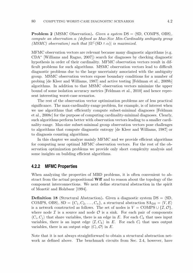
80 COMPUTING WORST-CASE DIAGNOSTIC SCENARIOS 4.2
Problem 2 (MSMC Observation). Given a system DS = 〈SD, COMPS, OBS〉,compute an observation α (defined as Max-Size Min-Cardinality ambiguity group(MSMC) observation) such that |Ω≤(SD ∧ α)| is maximized.
MFMC observation vectors are relevant because many diagnostic algorithms (e.g.CDA∗ [Williams and Ragno, 2007]) search for diagnoses by checking diagnostichypothesis in order of their cardinality. MFMC observation vectors result in dif-ficult problems for such algorithms. MSMC observation vectors lead to difficultdiagnostic problems due to the large uncertainty associated with the ambiguitygroup. MSMC observation vectors expose boundary conditions for a number ofprobing [de Kleer and Williams, 1987] and active testing [Feldman et al., 2009b]algorithms. In addition to that MSMC observation vectors minimize the upperbound of some isolation accuracy metrics [Feldman et al., 2010] and hence repre-sent interesting worst-case scenarios.
The rest of the observation vector optimization problems are of less practicalsignificance. The max-cardinality-range problem, for example, is of interest whenwe use algorithms that efficiently compute subset-minimal diagnoses [Feldmanet al., 2008c] for the purpose of computing cardinality-minimal diagnoses. Clearly,such algorithms perform better with observation vectors leading to a smaller cardi-nality-range. Max-size subset-minimal group observation vectors pose challengesto algorithms that compute diagnostic entropy [de Kleer and Williams, 1987] orto diagnosis counting algorithms.
In this chapter we analyze mainly MFMC and we provide efficient algorithmsfor computing near optimal MFMC observation vectors. For the rest of the ob-servation optimization problems we provide only short complexity analysis andsome insights on building efficient algorithms.
4.2.2 MFMC Properties
When analyzing the properties of MBD problems, it is often convenient to ab-stract from the actual propositional Wff and to reason about the topology of thecomponent interconnections. We next define structural abstraction in the spiritof Mozetic and Holzbaur [1994].
Definition 18 (Structural Abstraction). Given a diagnostic system DS = 〈SD,COMPS, OBS〉, SD = C1, C2, . . . , Cn, a structural abstraction SADS = 〈V,E〉is a network constructed as follows. The set of nodes is V = COMPS ∪ I,O,where node I is a source and node O is a sink. For each pair of components〈Ci, Cj〉 that share variables, there is an edge in E. For each Ck that uses inputvariables, there is an input edge 〈I, Ck〉 in E. For each Cl that uses outputvariables, there is an output edge 〈Cl,O〉 in E.
Note that it is not always straightforward to obtain a structural abstraction net-work as defined above. The benchmark circuits from Sec. 2.4, however, have
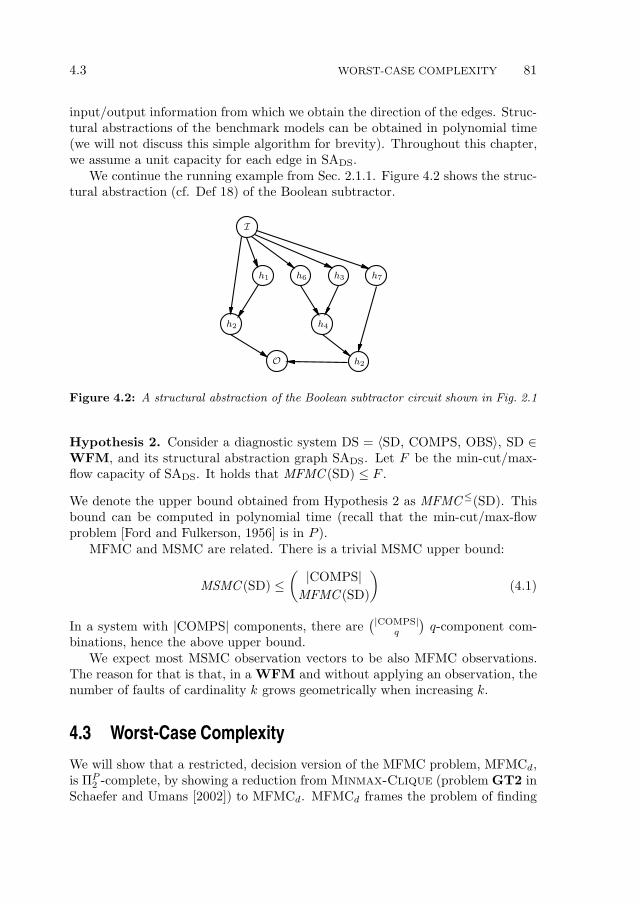
4.3 WORST-CASE COMPLEXITY 81
input/output information from which we obtain the direction of the edges. Struc-tural abstractions of the benchmark models can be obtained in polynomial time(we will not discuss this simple algorithm for brevity). Throughout this chapter,we assume a unit capacity for each edge in SADS.
We continue the running example from Sec. 2.1.1. Figure 4.2 shows the struc-tural abstraction (cf. Def 18) of the Boolean subtractor.
h7h1 h3h6
h4h2
O h2
I
Figure 4.2: A structural abstraction of the Boolean subtractor circuit shown in Fig. 2.1
Hypothesis 2. Consider a diagnostic system DS = 〈SD, COMPS, OBS〉, SD ∈WFM, and its structural abstraction graph SADS. Let F be the min-cut/max-flow capacity of SADS. It holds that MFMC (SD) ≤ F .
We denote the upper bound obtained from Hypothesis 2 as MFMC≤(SD). Thisbound can be computed in polynomial time (recall that the min-cut/max-flowproblem [Ford and Fulkerson, 1956] is in P ).
MFMC and MSMC are related. There is a trivial MSMC upper bound:
MSMC (SD) ≤( |COMPS|
MFMC (SD)
)(4.1)
In a system with |COMPS| components, there are(|COMPS|
q
)q-component com-
binations, hence the above upper bound.We expect most MSMC observation vectors to be also MFMC observations.
The reason for that is that, in a WFM and without applying an observation, thenumber of faults of cardinality k grows geometrically when increasing k.
4.3 Worst-Case Complexity
We will show that a restricted, decision version of the MFMC problem, MFMCd,is ΠP
2 -complete, by showing a reduction from Minmax-Clique (problem GT2 inSchaefer and Umans [2002]) to MFMCd. MFMCd frames the problem of finding
82 COMPUTING WORST-CASE DIAGNOSTIC SCENARIOS 4.3
an observation α that isolates a cardinality-minimal diagnosis ω of cardinality atleast k.
Problem 3 (MFMCd). Given a system DS = 〈SD, COMPS, OBS〉 and a con-stant k > 0, does there exist an observation α and a health assignment ω suchthat minω|=SD∧α |ω| ≥ k.We next show the complexity of the MFMCd problem.
Theorem 4. MFMCd is ΠP2 -complete.1
Proof.
1. It is easy to see that MFMCd is in ΠP2 , since it is solvable by a polynomial-
time nondeterministic machine with the use of an NP-complete oracle. Themachine chooses nondeterministically an observation α and checks with anNP-hard algorithm whether ∃ω : SD ∧ α ∧ ω 6|=⊥, |ω| < k.
2. We now show a reduction from the ΠP2 -complete problem Minmax-Clique
(problem GT2 in Schaefer and Umans [2002]).
Minmax-Clique is denoted by a graphG = (V,E), a partition (Vi,j)i∈I,j∈J
of V , an integer κ, a function t : I → J , and χt is the size of the largest cliquein G restricted to
⋃i∈I (Vi,t(i)). In other words, we can denote χt(G) =
mint maxχ|χ| : χ ⊆ V is a clique in Gt. Gt denotes the induced subgraph
of G on the vertex set Vi =⋃I
i=1 Vi,t(i).
Given the partition, |V | = I · J = n; hence V = v1,1, v1,2, · · · , v1,J ,v2,1, · · · , v2,J , · · · , vI,J. Partition i is given by vi,1, vi,2, · · · , vi,J fori = 1, 2, · · · , I.We assume that in MFMCd, there are I health variables, each of which hasJ possible (abnormal) health values, i.e., health variable k has values givenby hk,1, hk,2, · · · , hk,J, k = 1, 2, · · · , I. Hence our space of possible healthvalues is given by H = h1,1, h1,2, · · · , h1,J , h2,1, · · · , h2,J , · · · , hI,J.We construct a CNF formula f from G as follows.
Variables The variables in f are as follows:
• For each vertex vi,j , introduce a variable hvi,j(the semantics is that
hvi,jis true if vi,j is in the clique, and the only literals occurring
in a clique χ are health literals).
• For each i = 1, 2, · · · , I, j = 1, 2, · · · , J , and k = 0, 1, 2, · · · , κ,introduce a variable Yi,j,k.
The second set of variables ensures that Yi,j,k is true if there are atleast k true variables in the set hv1,1
, . . . , hv1,J, hv2,1
, . . . , hvI,J.
1The proof of this theorem first appeared in Provan [2008]. The material in this chapter isbased on the joint paper submitted to Journal of Artificial Intelligence.
4.4 SYSTEM DESCRIPTION SIMPLIFICATIONS 83
Clauses The clauses in f are as follows:
• For each pair of vertices u, v ∈ G having no edge (u, v), add aclause ¬hv ∨ ¬hu to f .2
• For each i = 1, 2, . . . , I, j = 1, 2, . . . , J and k = 1, 2, . . . , κ, addclause Yi−1,j,k ∨ (Yi−1,j,k−1 ∧ hvi,j
).
• For each i = 1, 2, . . . , I, j = 1, 2, . . . , J , add clauses enforcingYi,j,0 = true.
• For each k = 1, 2, . . . , κ, add clauses enforcing Y0,0,k = false.
• Finally, add a clause containing just the variable YI,J,κ.
The above reduction clearly can be computed in polynomial time. Next weverify that the reduction is correct.
⇒ Suppose G has a clique χt of size κ. If this is true, then in f we mustassign true to the variables hv such that v ∈ χt, and false to the othervariables. We also assign true to those Yi,j,k’s such that there are at least ktrue variables in hv1
, hv2, . . . , hvi
, and we assign false to the other Yi,j,k’s.This gives a satisfying assignment for f .
Further, under the partition function t : I → J , χt(G) = mint maxχ|χ| :χ ⊆ V . This corresponds in our satisfying assignment in f to there existingminω|=f∧α |ω| = κ, since every node in χt(G) consists of a health literalfrom a different partition, i.e., it consists of a minimal diagnosis ω such that|ω| = κ.
⇐ Suppose f has a satisfying assignment. Let χ = v : hv is assigned true.Then χ is a clique because for any pair of vertices u, v ∈ χ, there cannot bea clause ¬hv ∨ ¬hu in f (because such a clause would not be satisfied), sothere must be an edge (u, v) ∈ G. χ has size κ or more because YI,J,κ mustbe true.
Further, a satisfying assignment in f must correspond to there existingχt(G) = mint maxχ|χ| : χ ⊆ V , since under the satisfying assignment wehave minω|=f∧α |ω| = κ, and every node in χt(G) consists of a health literalfrom a different partition, i.e., it consists of a minimal diagnosis ω such that|ω| = κ.
4.4 System Description Simplifications
The complexity of computing MFMC is exponential in the number of compo-nents. Therefore, any reduction in number of components which does not affectMFMC (SD) provides significant computational advantage. Consider again the
2At this point, the satisfying assignments to f correspond to cliques in G.
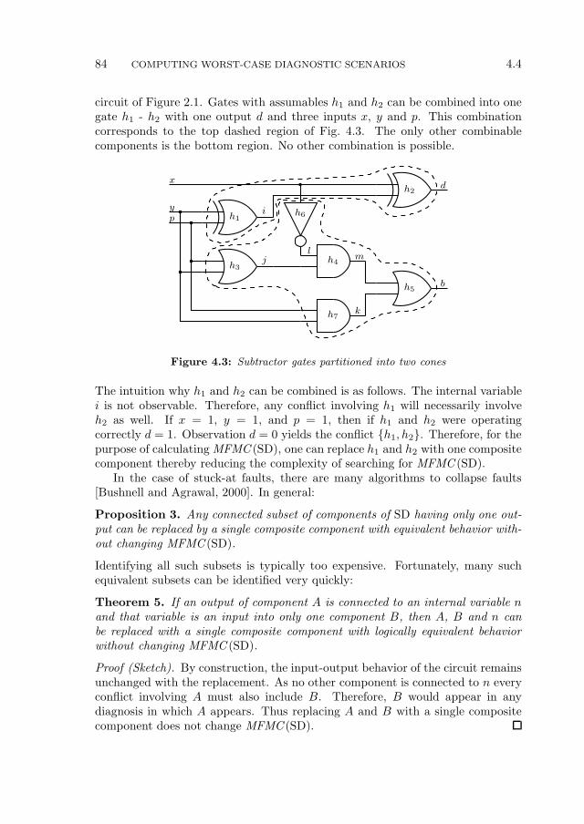
84 COMPUTING WORST-CASE DIAGNOSTIC SCENARIOS 4.4
circuit of Figure 2.1. Gates with assumables h1 and h2 can be combined into onegate h1 - h2 with one output d and three inputs x, y and p. This combinationcorresponds to the top dashed region of Fig. 4.3. The only other combinablecomponents is the bottom region. No other combination is possible.
h2d
h6yp h1
h3h4j
i
h5
h7
x
m
k
b
l
Figure 4.3: Subtractor gates partitioned into two cones
The intuition why h1 and h2 can be combined is as follows. The internal variablei is not observable. Therefore, any conflict involving h1 will necessarily involveh2 as well. If x = 1, y = 1, and p = 1, then if h1 and h2 were operatingcorrectly d = 1. Observation d = 0 yields the conflict h1, h2. Therefore, for thepurpose of calculating MFMC (SD), one can replace h1 and h2 with one compositecomponent thereby reducing the complexity of searching for MFMC (SD).
In the case of stuck-at faults, there are many algorithms to collapse faults[Bushnell and Agrawal, 2000]. In general:
Proposition 3. Any connected subset of components of SD having only one out-put can be replaced by a single composite component with equivalent behavior with-out changing MFMC (SD).
Identifying all such subsets is typically too expensive. Fortunately, many suchequivalent subsets can be identified very quickly:
Theorem 5. If an output of component A is connected to an internal variable nand that variable is an input into only one component B, then A, B and n canbe replaced with a single composite component with logically equivalent behaviorwithout changing MFMC (SD).
Proof (Sketch). By construction, the input-output behavior of the circuit remainsunchanged with the replacement. As no other component is connected to n everyconflict involving A must also include B. Therefore, B would appear in anydiagnosis in which A appears. Thus replacing A and B with a single compositecomponent does not change MFMC (SD).

4.4 SYSTEM DESCRIPTION SIMPLIFICATIONS 85
For example component h1, variable i and component h2 of Fig. 4.3 can be re-placed with a single component with inputs x, y and p and output d. By iterativelyapplying the preceding theorem the number of components can be significantlyreduced without changing MFMC (SD). The combined h1 − h2(h1,2) componentis described by the following propositional Wff :
h1,2 ⇒ [i⇔ ¬ (y ⇔ p)] ∧ [d⇔ ¬ (x⇔ i)]
Algorithm 5 demonstrates how to quickly identify cones. The approach is similarto that of [Siddiqi and Huang, 2007] and yields equivalent results. Algorithm 5uses the notion of dominated sets. A dominated set of a component g (G[g]) isdefined as the set of components X such that any path from a component in Xto any system output in OUT goes through g. A dominated set is also defined asa cone. We have seen in Theorem 5 that combining all the assumable variablesin each cone preserves the MFMC value.
Algorithm 5 An algorithm for computing cones
1: function ComputeCones(DS, IN, OUT) returns a set of sets
inputs: DS, a diagnostic system (DS = 〈SD,COMPS,OBS〉)IN, OUT, variable sets (IN ∪OUT = OBS, IN ∩OUT = ∅)
local variables: terminate, Boolean flagS, stackg, d1, d2, . . . , dn, component variables (n = |COMPS|)G, set of sets, (G is indexed by component variable,|G| = |COMPS|)
2: repeat
3: terminate ← T
4: Push(S,OUT)5: while g ← Pop(S) do
6: d1, d2, . . . , dm ← GetDrivenComponents(g)7: if G[d1] ∩ G[d2] ∩ · · · ∩ G[dm] 6= ∅ then
8: terminate ← F
9: end if
10: G[g]← g ∪ (G[d1] ∩ G[d2] ∩ · · · ∩ G[dm])11: Push(S,GetDrivingComponents(g))12: end while
13: until terminate14: returnRemoveSubsumptions(G)15: end function
The idea of Alg. 5 is to start from the system outputs OUT and greedily identifycones. The cone identification is repeated until no further change in the dominatedsets is achieved (lines 7 – 9). A dominated set is computed as the intersection of

86 COMPUTING WORST-CASE DIAGNOSTIC SCENARIOS 4.5
the dominated sets of all driving components (a component x drives a componenty is an output of x is connected to an input of y). A gate always dominates itself.
Algorithm 5 uses a stack S (and the auxiliary subroutines Push and Pop)to store the gates whose dominated sets are scheduled for update. Note thatAlgorithm 5 does not satisfy any optimality criteria for the computed cones, i.e.,the order in which output gates in line 4 and driving components in line 11 arepushed to S is not specified making Alg 5 non-deterministic.
As the properties of cones and Alg. 5 are well-studied we will skip the issues oftermination and complexity. Extensive experimentation (cf. Sec. 4.6) shows thatAlg. 5 is very efficient even for large circuits and produces results which preservethe MFMC values.
Important properties which improve running time dramatically on many cir-cuits are:
• Suppose SD can be divided into two SD1 and SD2 such they share no internalvariables. In this case, MFMC calculation is greatly simplified:
MFMC (SD) = MFMC (SD1) + MFMC (SD2)
Similarly,MSMC (SD) = MSMC (SD1)×MSMC (SD2)
The two formulae above follow from the fact that the global set of diagnosesof two independent systems is the Cartesian product of the diagnoses of theindividual systems.
• Let SD|i=x represent the system SD with input i set to x and the resultingcircuit simplified by removing irrelevant components.
MFMC (SD) = max(MFMC (SD|i=0),MFMC (SD|i=1))
• If all of the inputs of a components are fed directly from the inputs (and noother component is driven by those inputs), then this set of inputs can bereduced to one and the component replaced by a buffer.
4.5 MFMC Algorithm
A naıve approach to compute MFMC (SD) is to consider an exhaustive algorithm.Such an algorithm would enumerate all the 2|OBS| instantiations of the variablesin OBS; one can easily show that only an assignments to all variables in OBS canbe an MFMC observation vector as the MFMC problem is monotonic in respectto partial observations. For each full instantiation α, an MBD oracle computesthe associated minimal fault cardinality.
Taking this exhaustive approach in our running example, we compute thatMFMC (SD) = 2 and that there is a total of 9 observation vectors discerning a
4.5 MFMC ALGORITHM 87
minimal-cardinality diagnosis of 2 faults (α2 from Sec. 2.1 is an example of suchan observation vector). From all the 32 possible observation vectors, there are 7,16, and 9 observation vectors leading to a nominal, single-fault, and double-faultminimal-cardinality diagnosis, respectively.
Of course, such an exhaustive algorithm is computationally infeasible. Wepropose a stochastic method that trades optimality for a huge speedup, allowingvery-high-k observations to be computed for very large circuits. Despite the in-herent suboptimality of the stochastic approach, we will see in the experimentalsection of this chapter that, for smaller circuits from the 74XXX family, usingMiranda results in optimal observation vectors. The success of our stochasticapproach is that, as we will see in the experimental section, landscapes of typicalMFMC search problems have many optima which are close or equal to the globaloptimum.
Alg. 6 assumes that an “all-healthy”mode of all assumable variables allows aninput assignment to be propagated to all outputs. This is typical for health-modelsof digital circuits and for diagnosis problems.Alg. 6 performs L independent attempts (restarts), each one starting from a ran-dom observation vector that corresponds to nominal health. This random startingpoint is computed as follows. First, the RandomInputs function assigns to eachvariable in IN a random value, the resulting term is then assigned to β. Theserandom inputs are then fed to the ComputeOutputs subroutine which assignshealthy values to the assumable variables, and computes the values of the vari-ables in the output set OUT. This can be done by using a suitable propagationmethod like Binary Constraint Propagation [Zabih and McAllester, 1988]. Theresult of ComputeOutputs is then assigned to γ.
Starting from this initial candidate observation β∧γ, Alg. 6 attempts to reducethe cardinality of a minimal-diagnosis consistent with an observation vector by“flipping” the values of the output variables. This is achieved by the auxiliaryfunction FlipLiteral. At each step, the cardinality of the minimal-cardinalitydiagnosis is computed by a call to the MBD oracle FindMCDiagnosis. Theobservation leading to the highest-cardinality fault is stored and returned as aresult of the MFMC computation.
Our MBD oracle must be carefully designed, since computing minimal cardi-nality diagnoses has a very high worst-case complexity: given arbitrary propo-sitional theories in SD, the complexity of finding the cardinality of a minimal-cardinality diagnosis is ΣP
2 -hard [Eiter and Gottlob, 1995]. The complexity de-creases by imposing restrictions on the class of admissible system models, e.g.,models with ignorance of abnormal behavior [de Kleer et al., 1992a], Horn the-ories, etc. For improving the speed of MBD in the average case, the literaturehas discussed a number of learning [Williams and Ragno, 2007] or approximation[Feldman et al., 2008c] techniques. Although our MFMC algorithm is transpar-ent to the choice of the minimal-diagnosis oracle, the choice can be optimizedwhen additional information on the specific properties of the system descriptionsis available. In our implementation we use Safari (cf. Chapter 3) as a function for
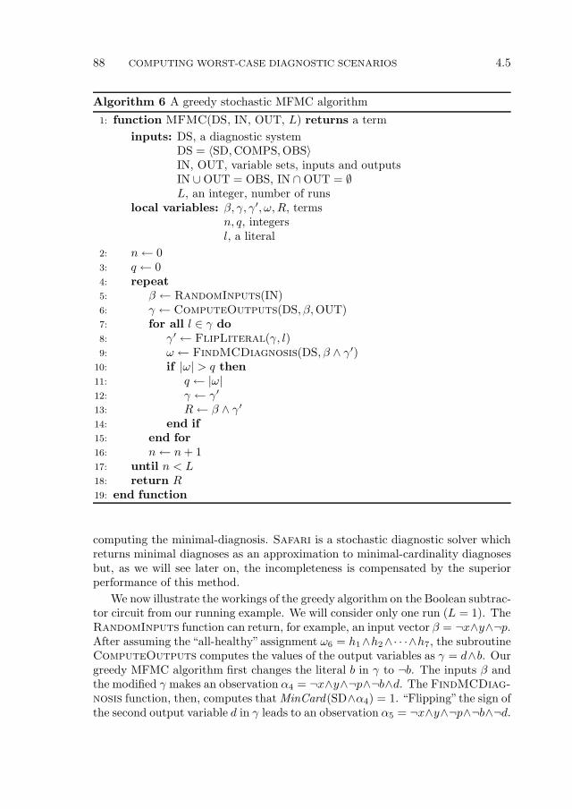
88 COMPUTING WORST-CASE DIAGNOSTIC SCENARIOS 4.5
Algorithm 6 A greedy stochastic MFMC algorithm
1: function MFMC(DS, IN, OUT, L) returns a term
inputs: DS, a diagnostic systemDS = 〈SD,COMPS,OBS〉IN, OUT, variable sets, inputs and outputsIN ∪OUT = OBS, IN ∩OUT = ∅L, an integer, number of runs
local variables: β, γ, γ′, ω,R, termsn, q, integersl, a literal
2: n← 03: q ← 04: repeat
5: β ← RandomInputs(IN)6: γ ← ComputeOutputs(DS, β,OUT)7: for all l ∈ γ do
8: γ′ ← FlipLiteral(γ, l)9: ω ← FindMCDiagnosis(DS, β ∧ γ′)
10: if |ω| > q then
11: q ← |ω|12: γ ← γ′
13: R← β ∧ γ′14: end if
15: end for
16: n← n+ 117: until n < L18: return R19: end function
computing the minimal-diagnosis. Safari is a stochastic diagnostic solver whichreturns minimal diagnoses as an approximation to minimal-cardinality diagnosesbut, as we will see later on, the incompleteness is compensated by the superiorperformance of this method.
We now illustrate the workings of the greedy algorithm on the Boolean subtrac-tor circuit from our running example. We will consider only one run (L = 1). TheRandomInputs function can return, for example, an input vector β = ¬x∧y∧¬p.After assuming the “all-healthy”assignment ω6 = h1∧h2∧· · ·∧h7, the subroutineComputeOutputs computes the values of the output variables as γ = d∧b. Ourgreedy MFMC algorithm first changes the literal b in γ to ¬b. The inputs β andthe modified γ makes an observation α4 = ¬x∧y∧¬p∧¬b∧d. The FindMCDiag-
nosis function, then, computes that MinCard(SD∧α4) = 1. “Flipping”the sign ofthe second output variable d in γ leads to an observation α5 = ¬x∧y∧¬p∧¬b∧¬d.
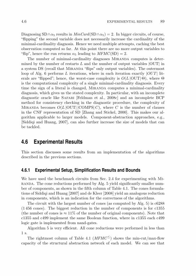
4.6 EXPERIMENTAL RESULTS 89
Diagnosing SD∧α5 results in MinCard(SD∧α5) = 2. In bigger circuits, of course,“flipping” the second variable does not necessarily increase the cardinality of theminimal-cardinality diagnosis. Hence we need multiple attempts, caching the bestobservation computed so far. At this point there are no more output variables to“flip”, hence the run returns α5 leading to MFMC (SD) = 2.
The number of minimal-cardinality diagnoses Miranda computes is deter-mined by the number of restarts L and the number of output variables |OUT| ina system DS (recall that Miranda “flips” only output variables). The outermostloop of Alg. 6 performs L iterations, where in each iteration exactly |OUT | lit-erals are “flipped”; hence, the worst-case complexity is O(L |OUT|Θ), where Θis the computational complexity of a single minimal-cardinality diagnosis. Everytime the sign of a literal is changed, Miranda computes a minimal-cardinalitydiagnosis, which gives us the stated complexity. In particular, with an incompletediagnostic oracle like Safari [Feldman et al., 2008c] and an incomplete BCPmethod for consistency checking in the diagnostic procedure, the complexity ofMiranda becomes O(L |OUT| |COMPS|C), where C is the number of clausesin the CNF representation of SD [Zhang and Stickel, 2000]. This makes our al-gorithm applicable to larger models. Component-abstraction approaches, e.g.,[Siddiqi and Huang, 2007], can also further increase the size of models that canbe tackled.
4.6 Experimental Results
This section discusses some results from an implementation of the algorithmsdescribed in the previous sections.
4.6.1 Experimental Setup, Simplification Results and Bounds
We have used the benchmark circuits from Sec. 2.4 for experimenting with Mi-
randa. The cone reductions performed by Alg. 5 yield significantly smaller num-ber of components, as shown in the fifth column of Table 4.1. The cones formula-tions of Siddiqi and Huang [2007] and de Kleer [2008] yield an analogous reductionin components, which is an indication for the correctness of the algorithms.
The circuit with the largest number of cones (as computed by Alg. 5) is c6288(1 456 cones). The biggest reduction in the number of components is for c1355(the number of cones is ≈ 11% of the number of original components). Note thatc1355 and c499 implement the same Boolean function, where in c1355 each c499logic gate is implemented from nand-gates.
Algorithm 5 is very efficient. All cone reductions were performed in less than1 s.
The rightmost column of Table 4.1 (MFMC≤) shows the min-cut/max-flowcapacity of the structural abstraction network of each model. We can see that
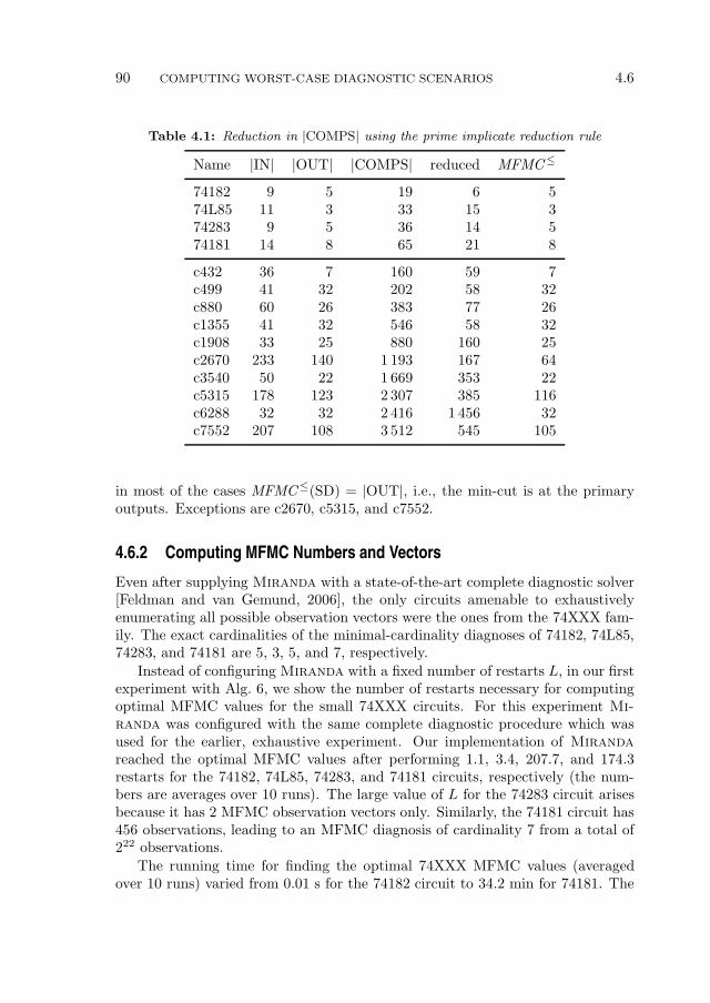
90 COMPUTING WORST-CASE DIAGNOSTIC SCENARIOS 4.6
Table 4.1: Reduction in |COMPS| using the prime implicate reduction rule
Name |IN| |OUT| |COMPS| reduced MFMC≤
74182 9 5 19 6 574L85 11 3 33 15 374283 9 5 36 14 574181 14 8 65 21 8
c432 36 7 160 59 7c499 41 32 202 58 32c880 60 26 383 77 26c1355 41 32 546 58 32c1908 33 25 880 160 25c2670 233 140 1 193 167 64c3540 50 22 1 669 353 22c5315 178 123 2 307 385 116c6288 32 32 2 416 1 456 32c7552 207 108 3 512 545 105
in most of the cases MFMC≤(SD) = |OUT|, i.e., the min-cut is at the primaryoutputs. Exceptions are c2670, c5315, and c7552.
4.6.2 Computing MFMC Numbers and Vectors
Even after supplying Miranda with a state-of-the-art complete diagnostic solver[Feldman and van Gemund, 2006], the only circuits amenable to exhaustivelyenumerating all possible observation vectors were the ones from the 74XXX fam-ily. The exact cardinalities of the minimal-cardinality diagnoses of 74182, 74L85,74283, and 74181 are 5, 3, 5, and 7, respectively.
Instead of configuring Miranda with a fixed number of restarts L, in our firstexperiment with Alg. 6, we show the number of restarts necessary for computingoptimal MFMC values for the small 74XXX circuits. For this experiment Mi-
randa was configured with the same complete diagnostic procedure which wasused for the earlier, exhaustive experiment. Our implementation of Miranda
reached the optimal MFMC values after performing 1.1, 3.4, 207.7, and 174.3restarts for the 74182, 74L85, 74283, and 74181 circuits, respectively (the num-bers are averages over 10 runs). The large value of L for the 74283 circuit arisesbecause it has 2 MFMC observation vectors only. Similarly, the 74181 circuit has456 observations, leading to an MFMC diagnosis of cardinality 7 from a total of222 observations.
The running time for finding the optimal 74XXX MFMC values (averagedover 10 runs) varied from 0.01 s for the 74182 circuit to 34.2 min for 74181. The

4.6 EXPERIMENTAL RESULTS 91
long running time for reaching the MFMC of 74181 model comes from the poorperformance of the complete diagnostic procedure we have used (despite the factthat we have employed a state-of-the-art solver). This is not surprising, consid-ering that, with traditional MBD algorithms for computing minimal-cardinalitydiagnoses, the computational cost of finding a k-minimal-cardinality diagnosisincreases with k.
Consider an MFMC algorithm that uses the GDE [de Kleer and Williams,1987] algorithm as a diagnostic oracle. GDE first constructs all minimal con-flicts and then constructs the minimal diagnoses from the minimal conflicts. Thisapproach constructs far more conflicts than are necessary to find one minimal-cardinality diagnosis, and hence its cardinality. If there are a large number ofminimal diagnoses, most of this is useless work. The c6288 circuit can never beanalyzed by this approach as it yields an exponential number of minimal conflicts.These result from its inherently parallel structure illustrated in Fig. 4.4. Each boxin Fig. 4.4 represents a 2-bit adder (there are 240 of them). In addition to that,c6288 uses an and-gate that connects the two least significant inputs to the outputo0 (this and-gate is not shown in Fig. 4.4).
o0o1
o2
o3
o4
o5
o6
o7
o8
o9
o10
o11
o12
o13
o14
o15
half adder
full adder
o16o18o20o22o24o26o28 o27 o25 o23 o21 o19 o17o29o30o31
Figure 4.4: The most difficult to analyze circuit from the ISCAS85 test suite. It is a16 × 16 bit parallel multiplier built out of half and full adders.
The MFMC of the c6288 circuit can be determined by visually inspecting thecircuit diagram (cf. Fig. 4.4). We have brute-forced a 3-bit multiplier, and itsMFMC value is 3. The circuit in Fig. 4.4 can be partitioned by cutting 16 con-nections. Hence, we hypothesize, that MFMC (c6288) = 16. Furthermore, wehypothesize that the MFMC value of a regular, n-bit multiplier is n.
Given a system DS, we denote as g(DS) the pdf of the minimal-cardinalitiesof the diagnoses of all observations in DS. Figure 4.5 shows a histogram of thetrue minimal-diagnosis cardinalities for the four 74XXX circuits for which we have
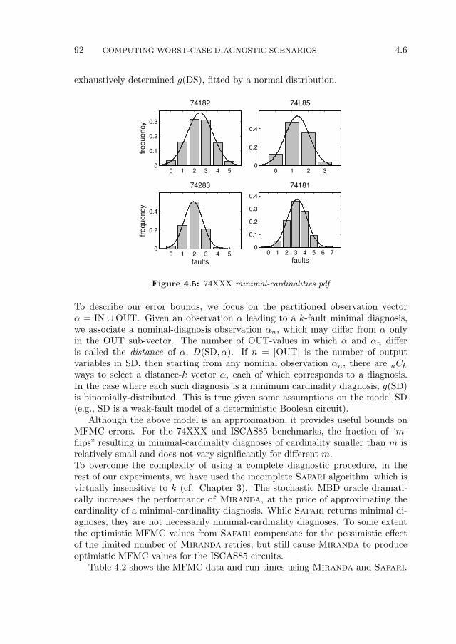
92 COMPUTING WORST-CASE DIAGNOSTIC SCENARIOS 4.6
exhaustively determined g(DS), fitted by a normal distribution.
0 1 2 3 4 50
0.1
0.2
0.3
74182
frequency
0 1 2 30
0.2
0.4
74L85
0 1 2 3 4 50
0.2
0.4
74283
faults
frequency
0 1 2 3 4 5 6 70
0.1
0.2
0.3
0.4
74181
faults
Figure 4.5: 74XXX minimal-cardinalities pdf
To describe our error bounds, we focus on the partitioned observation vectorα = IN ∪ OUT. Given an observation α leading to a k-fault minimal diagnosis,we associate a nominal-diagnosis observation αn, which may differ from α onlyin the OUT sub-vector. The number of OUT-values in which α and αn differis called the distance of α, D(SD, α). If n = |OUT| is the number of outputvariables in SD, then starting from any nominal observation αn, there are nCk
ways to select a distance-k vector α, each of which corresponds to a diagnosis.In the case where each such diagnosis is a minimum cardinality diagnosis, g(SD)is binomially-distributed. This is true given some assumptions on the model SD(e.g., SD is a weak-fault model of a deterministic Boolean circuit).
Although the above model is an approximation, it provides useful bounds onMFMC errors. For the 74XXX and ISCAS85 benchmarks, the fraction of “m-flips” resulting in minimal-cardinality diagnoses of cardinality smaller than m isrelatively small and does not vary significantly for different m.To overcome the complexity of using a complete diagnostic procedure, in therest of our experiments, we have used the incomplete Safari algorithm, which isvirtually insensitive to k (cf. Chapter 3). The stochastic MBD oracle dramati-cally increases the performance of Miranda, at the price of approximating thecardinality of a minimal-cardinality diagnosis. While Safari returns minimal di-agnoses, they are not necessarily minimal-cardinality diagnoses. To some extentthe optimistic MFMC values from Safari compensate for the pessimistic effectof the limited number of Miranda retries, but still cause Miranda to produceoptimistic MFMC values for the ISCAS85 circuits.
Table 4.2 shows the MFMC data and run times using Miranda and Safari.
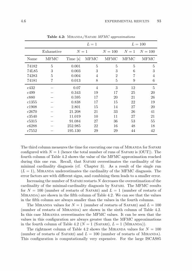
4.6 EXPERIMENTAL RESULTS 93
Table 4.2: Miranda/Safari MFMC approximations
L = 1 L = 100
Exhaustive N = 1 N = 100 N = 1 N = 100
Name MFMC Time [s] MFMC MFMC MFMC MFMC
74182 5 0.001 5 5 5 574L85 3 0.003 3 3 6 374283 5 0.004 4 2 7 474181 7 0.013 8 5 9 6
c432 − 0.07 4 3 12 5c499 − 0.343 19 17 25 20c880 − 0.595 17 20 21 26c1355 − 0.838 17 15 22 19c1908 − 2.801 15 14 27 20c2670 − 21.208 21 33 26 41c3540 − 11.019 10 11 27 21c5315 − 91.084 27 36 53 55c6288 − 252.985 22 16 48 18c7552 − 195.130 29 29 44 42
The third column measures the time for executing one run of Miranda for Safari
configured with N = 1 (hence the total number of runs of Safari is |OUT|). Thefourth column of Table 4.2 shows the value of the MFMC approximation reachedduring this one run. Recall, that Safari overestimates the cardinality of theminimal cardinality diagnosis (cf. Chapter 3). As a result of the single run(L = 1), Miranda underestimates the cardinality of the MFMC diagnosis. Theerror factors are with different signs, and combining them leads to a smaller error.
Increasing the number of Safari restartsN decreases the overestimation of thecardinality of the minimal-cardinality diagnosis by Safari. The MFMC resultsfor N = 100 (number of restarts of Safari) and L = 1 (number of restarts ofMiranda) are shown in the fifth column of Table 4.2. We can see that the valuesin the fifth column are always smaller than the values in the fourth columns.
The Miranda values for N = 1 (number of restarts of Safari) and L = 100(number of restarts of Miranda) are shown in the sixth column of Table 4.2.In this case Miranda overestimates the MFMC values. It can be seen that thevalues in this configuration are always greater than the MFMC approximationsin the fourth column of Table 4.2 (N = 1 (Safari), L = 1 (Miranda)).
The rightmost column of Table 4.2 shows the Miranda values for N = 100(number of restarts of Safari) and L = 100 (number of restarts of Miranda).This configuration is computationally very expensive. For the large ISCAS85
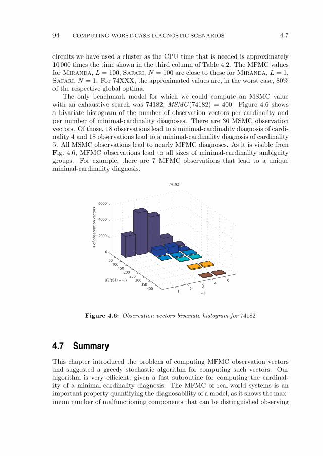
94 COMPUTING WORST-CASE DIAGNOSTIC SCENARIOS 4.7
circuits we have used a cluster as the CPU time that is needed is approximately10 000 times the time shown in the third column of Table 4.2. The MFMC valuesfor Miranda, L = 100, Safari, N = 100 are close to these for Miranda, L = 1,Safari, N = 1. For 74XXX, the approximated values are, in the worst case, 80%of the respective global optima.
The only benchmark model for which we could compute an MSMC valuewith an exhaustive search was 74182, MSMC (74182) = 400. Figure 4.6 showsa bivariate histogram of the number of observation vectors per cardinality andper number of minimal-cardinality diagnoses. There are 36 MSMC observationvectors. Of those, 18 observations lead to a minimal-cardinality diagnosis of cardi-nality 4 and 18 observations lead to a minimal-cardinality diagnosis of cardinality5. All MSMC observations lead to nearly MFMC diagnoses. As it is visible fromFig. 4.6, MFMC observations lead to all sizes of minimal-cardinality ambiguitygroups. For example, there are 7 MFMC observations that lead to a uniqueminimal-cardinality diagnosis.
50100
150200
250300
350400
12
34
5
0
2000
4000
6000
|!|
|Ω≤(SD ∧ !)|
# o
f o
bse
rvat
ion
ve
cto
rs
74182
Figure 4.6: Observation vectors bivariate histogram for 74182
4.7 Summary
This chapter introduced the problem of computing MFMC observation vectorsand suggested a greedy stochastic algorithm for computing such vectors. Ouralgorithm is very efficient, given a fast subroutine for computing the cardinal-ity of a minimal-cardinality diagnosis. The MFMC of real-world systems is animportant property quantifying the diagnosability of a model, as it shows the max-imum number of malfunctioning components that can be distinguished observing

4.7 SUMMARY 95
a set of variables. We have empirically demonstrated Miranda on a number of74XXX/ISCAS85 combinatorial circuits, computing the MFMC of these circuits.

96 COMPUTING WORST-CASE DIAGNOSTIC SCENARIOS 4.7

Chapter 5
A Model-Based Active Testing
Approach to Sequential Diagnosis
Model-based diagnostic reasoning often leads to a large number of diagnostichypotheses. The set of diagnoses can be reduced by taking into account extraobservations (passive monitoring), measuring additional variables (probing) orexecuting additional tests (sequential diagnosis/test sequencing). In this chap-ter we combine the above approaches, as well as from Automated Test PatternGeneration (ATPG) and Model-Based Diagnosis (MBD) into a framework calledFractal (FRamework for ACtive Testing ALgorithms). Apart from the inputsand outputs that connect a system to its environment, in active testing we con-sider additional input variables to which a sequence of test vectors can be supplied.We address the computationally hard problem of computing optimal control as-signments (as defined in Fractal) in terms of a greedy approximation algorithmcalled FractalG. We model the decrease in the number of remaining minimalcardinality diagnoses produced by an active testing algorithm as a geometric de-cay process and measure the algorithm’s performance in terms of the decay rate.FractalG employs approximation approaches, such as stochastic sampling forcomputing the expected number of remaining minimal cardinality diagnoses andgreedy search for computing the optimal control assignment, which results in acomputationally efficient method. We compare the optimality of FractalG tothat of two more Fractal algorithms: FractalA and FractalP. FractalA
is based on ATPG and sequential diagnosis while FractalP, although not anactive testing algorithm, provides a baseline for comparing the lower bound onthe number of reachable diagnoses for the Fractal algorithms. We empiricallyevaluate the trade-offs of the three Fractal algorithms by performing extensiveexperimentation on the ISCAS85/74XXX benchmark of combinational circuits.
97
98 AN ACTIVE TESTING APPROACH TO SEQUENTIAL DIAGNOSIS 5.1
5.1 Introduction
Combinational Model-Based Diagnosis (MBD) approaches [de Kleer and Wil-liams, 1987] often lead to a large number of diagnoses, in the worst-case, expo-nential in the number of components. Combining multiple sensor readings (obser-vation vectors) [Pietersma and van Gemund, 2006] helps in a limited number ofcases because the approach is inherently passive, i.e., there are situations in whichthe observations repeat themselves (for example, in systems that are stationary,pending a reconfiguration).
Sequential diagnosis algorithms [Shakeri, 1996] can be used as an alternativeto the above passive approach with better decay of the number of diagnostichypotheses. The decay rate depends on the tests and test dictionary matrix,and is bounded from below for tests with binary outcomes. Sequential diagnosisalgorithms suffer from a number of other limitations. Early approaches assumesingle-faults while multiple-fault sequential diagnosis is super-exponential (Σp
2 orharder) [Shakeri et al., 2000].
As observations (test outcomes) are not known in advance, the goal of a di-agnostician is to create a policy that minimizes the diagnostic uncertainty onaverage, i.e., one aims at minimizing the average depth of a test tree. Pattipatiand Alexandridis [1990] have shown that under certain conditions (e.g., unit testcosts and equal prior fault probabilities) one-step look-ahead policy leads to an op-timal average depth of the test tree while de Kleer et al. [1992b] have shown thatone-step look-ahead delivers good practical result for a range of combinationalcircuits.
As reliable component failure rates may be problematic to obtain, we assumeequally likely and small prior probabilities of failure and measure the diagnosticuncertainty as the number of Minimal Cardinality (MC) diagnoses. The latterapproach also has computational advantages. It can be shown that with equaland small prior probabilities of failure, the diagnostic entropy, e.g., as used byde Kleer and Williams [1987], can be computed directly from the number of MCdiagnoses.
The computational complexity of deterministic algorithms for sequential diag-nosis increases with respect to both the fault-cardinality and the number of tests(the size of the test dictionary). To enable performance to scale up to real-worldproblems, which may have high fault-cardinality and a large number of tests, wepropose FractalG–a low-cost greedy stochastic approach that maintains expo-nential decay of the number of MC diagnoses. Instead of assuming single faultsor timing out, FractalG may result in suboptimal but still exponential decay.
FractalG is specified within a formally-defined framework called Fractal
(FRamework for ACtive Testing ALgorithms). In Fractal, in addition to theinput (IN) and output (OUT) variables, we also discern control (CTL) variables.Controls are similar to inputs, except they can be modified by users while thesystem is connected to its environment. The use of models from first principlesand controls in Fractal allows us to eliminate the need of designing explicit tests
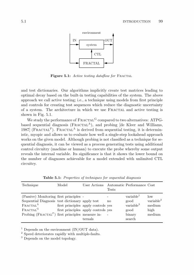
5.1 INTRODUCTION 99
FRACTAL
system
environment
IN OUT
CTL
Figure 5.1: Active testing dataflow for Fractal
and test dictionaries. Our algorithms implicitly create test matrices leading tooptimal decay based on the built-in testing capabilities of the system. The aboveapproach we call active testing; i.e., a technique using models from first principleand controls for creating test sequences which reduce the diagnostic uncertaintyof a system. The architecture in which we use Fractal and active testing isshown in Fig. 5.1.
We study the performance of FractalG compared to two alternatives: ATPG-based sequential diagnosis (FractalA), and probing [de Kleer and Williams,1987] (FractalP). FractalA is derived from sequential testing, it is determin-istic, myopic and allows us to evaluate how well a single-step lookahead approachworks on the given model. Although probing is not classified as a technique for se-quential diagnosis, it can be viewed as a process generating tests using additionalcontrol circuitry (machine or human) to execute the probe whereby some outputreveals the internal variable. Its significance is that it shows the lower bound onthe number of diagnoses achievable for a model extended with unlimited CTLcircuitry.
Table 5.1: Properties of techniques for sequential diagnosis
Technique Model User Actions AutomaticTests
Performance Cost
(Passive) Monitoring first principles - - variable1 lowSequential Diagnosis test dictionary apply test no good variable2
FractalA first principles apply controls yes variable3 mediumFractalG first principles apply controls yes good highProbing (FractalP) first principles measure in- - binary medium
ternals search
1 Depends on the environment (IN/OUT data).2 Speed deteriorates rapidly with multiple-faults.3 Depends on the model topology.
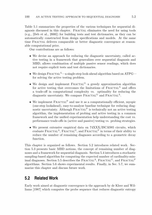
100 AN ACTIVE TESTING APPROACH TO SEQUENTIAL DIAGNOSIS 5.2
Table 5.1 summarizes the properties of the various techniques for sequential di-agnosis discussed in this chapter. Fractal eliminates the need for using tools(e.g., [Deb et al., 2000]) for building tests and test dictionaries, as they can beautomatically constructed from design specifications and models. At the sametime Fractal delivers comparable or better diagnostic convergence at reason-able computational price.
Our contributions are as follows:
• We devise an approach for reducing the diagnostic uncertainty, called ac-tive testing in a framework that generalizes over sequential diagnosis andMBD, allows combination of multiple passive sensor readings, which doesnot require explicit tests and test dictionaries.
• We design FractalA—a single-step look-ahead algorithm based on ATPG—for solving the active testing problem.
• We design and implement FractalG–a greedy approximation algorithmfor active testing that overcomes the limitations of FractalA and offersa trade-off in computational complexity vs. optimality for reducing thediagnostic uncertainty. We compare FractalG and FractalA.
• We implement FractalP and use it as a computationally efficient, myopic(one-step lookahead), easy-to-analyze baseline technique for reducing diag-nostic uncertainty. Although FractalP is technically not an active testingalgorithm, the implementation of probing and active testing in a commonframework and the unified experimentation help understanding the cost vs.performance trade-offs in (active and passive) testing vs. probing strategies.
• We present extensive empirical data on 74XXX/ISCAS85 circuits, whichevaluate FractalA, FractalG, and FractalP in terms of their ability toreduce the number of remaining diagnoses according to a geometric decayfunction.
This chapter is organized as follows. Section 5.2 introduces related work. Sec-tion 5.3 presents basic MBD notions, the concept of remaining number of diag-noses and a framework for sequential diagnosis. Section 5.4 introduces a stochasticsampling-based algorithm for computing the expected number of cardinality-min-imal diagnoses. Section 5.5 describes the FractalA, FractalG, and FractalP
algorithms. Section 5.6 shows experimental results. Finally, in Sec. 5.7, we sum-marize this chapter and discuss future work.
5.2 Related Work
Early work aimed at diagnostic convergence is the approach by de Kleer and Wil-liams [1987] which computes the probe sequence that reduces diagnostic entropy
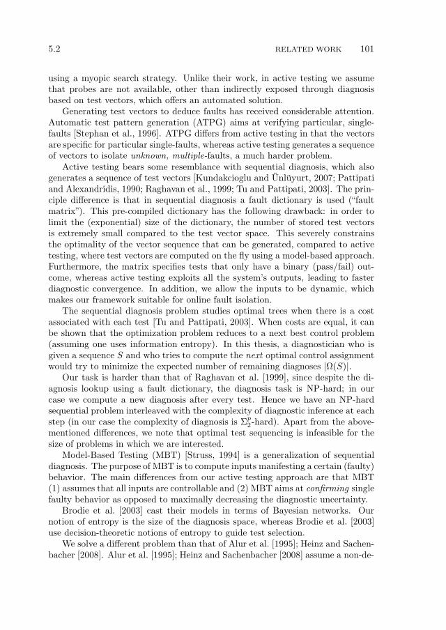
5.2 RELATED WORK 101
using a myopic search strategy. Unlike their work, in active testing we assumethat probes are not available, other than indirectly exposed through diagnosisbased on test vectors, which offers an automated solution.
Generating test vectors to deduce faults has received considerable attention.Automatic test pattern generation (ATPG) aims at verifying particular, single-faults [Stephan et al., 1996]. ATPG differs from active testing in that the vectorsare specific for particular single-faults, whereas active testing generates a sequenceof vectors to isolate unknown, multiple-faults, a much harder problem.
Active testing bears some resemblance with sequential diagnosis, which alsogenerates a sequence of test vectors [Kundakcioglu and Unluyurt, 2007; Pattipatiand Alexandridis, 1990; Raghavan et al., 1999; Tu and Pattipati, 2003]. The prin-ciple difference is that in sequential diagnosis a fault dictionary is used (“faultmatrix”). This pre-compiled dictionary has the following drawback: in order tolimit the (exponential) size of the dictionary, the number of stored test vectorsis extremely small compared to the test vector space. This severely constrainsthe optimality of the vector sequence that can be generated, compared to activetesting, where test vectors are computed on the fly using a model-based approach.Furthermore, the matrix specifies tests that only have a binary (pass/fail) out-come, whereas active testing exploits all the system’s outputs, leading to fasterdiagnostic convergence. In addition, we allow the inputs to be dynamic, whichmakes our framework suitable for online fault isolation.
The sequential diagnosis problem studies optimal trees when there is a costassociated with each test [Tu and Pattipati, 2003]. When costs are equal, it canbe shown that the optimization problem reduces to a next best control problem(assuming one uses information entropy). In this thesis, a diagnostician who isgiven a sequence S and who tries to compute the next optimal control assignmentwould try to minimize the expected number of remaining diagnoses |Ω(S)|.
Our task is harder than that of Raghavan et al. [1999], since despite the di-agnosis lookup using a fault dictionary, the diagnosis task is NP-hard; in ourcase we compute a new diagnosis after every test. Hence we have an NP-hardsequential problem interleaved with the complexity of diagnostic inference at eachstep (in our case the complexity of diagnosis is Σp
2-hard). Apart from the above-mentioned differences, we note that optimal test sequencing is infeasible for thesize of problems in which we are interested.
Model-Based Testing (MBT) [Struss, 1994] is a generalization of sequentialdiagnosis. The purpose of MBT is to compute inputs manifesting a certain (faulty)behavior. The main differences from our active testing approach are that MBT(1) assumes that all inputs are controllable and (2) MBT aims at confirming singlefaulty behavior as opposed to maximally decreasing the diagnostic uncertainty.
Brodie et al. [2003] cast their models in terms of Bayesian networks. Ournotion of entropy is the size of the diagnosis space, whereas Brodie et al. [2003]use decision-theoretic notions of entropy to guide test selection.
We solve a different problem than that of Alur et al. [1995]; Heinz and Sachen-bacher [2008]. Alur et al. [1995]; Heinz and Sachenbacher [2008] assume a non-de-

102 AN ACTIVE TESTING APPROACH TO SEQUENTIAL DIAGNOSIS 5.3
terministic system defined as an automaton. In contrast, our framework assumesa static system (plant model) for which we must compute a temporal sequence oftests to best isolate the diagnosis.
Esser and Struss [2007] also adopt an automaton framework for test genera-tion, except that, unlike Heinz and Sachenbacher [2008] or Alur et al. [1995], theytransform this automaton to a relational specification, and apply their frameworkto software diagnosis. This automaton-based framework accommodates more gen-eral situations than ours does, such as the possibility that the system’s state aftera transition may not be uniquely determined by the state before the transitionand the input, and/or the system’s state may be associated with several possibleobservations. In our MBD framework, a test consists of an instantiation of severalvariables, which corresponds to the notion of test sequence within the automatonframework of Heinz and Sachenbacher [2008].
A recent approach to active diagnosis is described by Kuhn et al. [2008], whereadditional test vectors are computed to optimize the diagnosis while the system (acopier) remains operational. Their work differs from ours in that plans (roughlyanalogous to test sequences) with a probability of failure T are computed stat-ically, and a plan remains unmodified even if it fails to achieve its desired goal(a manifestation of a failure with probability close to T ). Conversely, Fractal
dynamically computes next-best control settings in a game-like manner.Feldman et al. [2009b] discusses an early version of FractalG. This chapter
(1) generalizes Feldman et al. [2009b], (2) introduces FractalA and FractalP,(3) extends the experimental results, and (4) provides a comparison of the differentFractal approaches.
5.3 Concepts and Definitions
Our discussion starts by adopting relevant MBD notions. Central to MBD, amodel of an artifact is represented as a propositional Wff over a set of variablesV . We will discern four subsets of these variables: assumable, observable1, control,and internal variables. This gives us our initial definition:
Definition 19 (Active Testing System). An active testing system ATS is definedas ATS = 〈SD, COMPS, CTL, OBS〉, where SD is a propositional Wff over avariables set V , COMPS ∪ OBS ∪ CTL ⊆ V , and COMPS, OBS, and CTL aresets containing assumable, observable, and control variables, respectively.
The set of internal variables is denoted as INT, INT = V \COMPS∪OBS∪CTL.Throughout this chapter we assume that OBS, COMPS, and CTL are disjoint,and SD 6|=⊥. Sometimes it is convenient (but not necessary) to split OBS intonon-controllable inputs IN and outputs OUT (OBS = IN∪OUT, IN∩OUT = ∅).
1In the MBD literature the assumable variables are also referred to as “component”, “failure-mode”, or “health” variables. Observable variables are also called “measurable” variables.
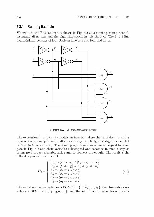
5.3 CONCEPTS AND DEFINITIONS 103
5.3.1 Running Example
We will use the Boolean circuit shown in Fig. 5.2 as a running example for il-lustrating all notions and the algorithm shown in this chapter. The 2-to-4 linedemultiplexer consists of four Boolean inverters and four and-gates.
b
a
io1
o2
o3
o4
h2
h3 h4
h1p
s
r
q
h5
h6
h7
h8
Figure 5.2: A demultiplexer circuit
The expression h⇒ (o⇔ ¬i) models an inverter, where the variables i, o, and hrepresent input, output, and health respectively. Similarly, an and-gate is modeledas h ⇒ (o⇔ i1 ∧ i2 ∧ i3). The above propositional formulae are copied for eachgate in Fig. 5.2 and their variables subscripted and renamed in such a way asto ensure a proper disambiguation and to connect the circuit. The result is thefollowing propositional model:
SD =
[h1 ⇒ (a⇔ ¬p)] ∧ [h2 ⇒ (p⇔ ¬r)][h3 ⇒ (b⇔ ¬q)] ∧ [h4 ⇒ (q ⇔ ¬s)]h5 ⇒ (o1 ⇔ i ∧ p ∧ q)h6 ⇒ (o2 ⇔ i ∧ r ∧ q)h7 ⇒ (o3 ⇔ i ∧ p ∧ s)h8 ⇒ (o4 ⇔ i ∧ r ∧ s)
(5.1)
The set of assumable variables is COMPS = h1, h2, . . . , h8, the observable vari-ables are OBS = a, b, o1, o2, o3, o4, and the set of control variables is the sin-

104 AN ACTIVE TESTING APPROACH TO SEQUENTIAL DIAGNOSIS 5.4
gleton CTL = i. Note the conventional selection of the sign of the “health”variables h1, h2, . . . , hn. Other authors use “ab” for abnormal.
5.3.2 Sequential Diagnosis
Throughout this chapter, we assume that the health of the system under test doesnot change during the test (i.e., the same inputs and a fault produce the sameoutputs) and call this assumption stationary health.
Lemma 8. Given a system ATS, a stationary health state for its components ω,and an observation sequence S, it follows that ω ∈ Ω(SD, α1) ∩ Ω(SD, α2) ∩ . . . ∩Ω(SD, αk).
Proof. The above statement follows immediately from the stationary health as-sumption and Def. 5.
Lemma 8 can be applied only in the cases in which all diagnoses are considered.If we compute subset-minimal diagnoses in a weak-fault model, for example, theintersection operator has to be redefined to handle subsumptions. To handle non-characterizing sets of diagnoses (e.g., MC or first m diagnoses), we provide thefollowing definition.
Definition 20 (Consistency-Based Intersection). Given a set of diagnoses D ofSD ∧ α, and a posteriori observation α′, the intersection of D with the diagnosesof SD∧ α′, denoted as Ω∩(D,α′), is defined as the set D′ (D′ ⊆ D) such that foreach ω ∈ D′ it holds that SD ∧ α′ ∧ ω 6|=⊥.
It is straightforward to generalize the above definition to an observation sequenceS.
Definition 21 (Remaining Minimal-Cardinality Diagnoses). Given a diagnosticsystem ATS and an observation sequence S, the set of remaining diagnoses Ω(S)is defined as Ω(S) = Ω∩(Ω∩(· · ·Ω∩(Ω≤(SD, α1), α2), · · · ), αk).
We use |Ω(S)| instead of the more precise diagnostic entropy as defined by deKleer et al. [de Kleer and Williams, 1987] and subsequent works, as this allowslow-complexity estimations (discussed in Sec. 5.4). In particular, if all diagnosesare of minimal-cardinality and the failure probability of each component is thesame, then the gain in the diagnostic entropy can be directly computed from|Ω(S)|.
5.4 Computing the Expected Number of MC Diagnoses
Active testing aims to minimize the expected number of diagnoses that resultfrom the possible set of outputs that may occur from a give control vector. Inthis section we present an algorithm to approximate this expectation.
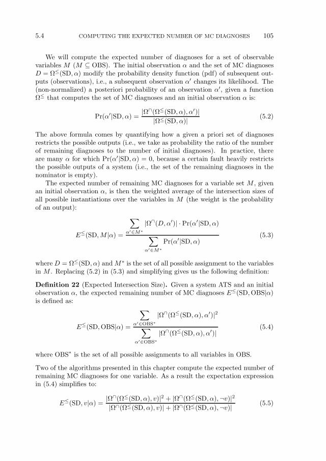
5.4 COMPUTING THE EXPECTED NUMBER OF MC DIAGNOSES 105
We will compute the expected number of diagnoses for a set of observablevariables M (M ⊆ OBS). The initial observation α and the set of MC diagnosesD = Ω≤(SD, α) modify the probability density function (pdf) of subsequent out-puts (observations), i.e., a subsequent observation α′ changes its likelihood. The(non-normalized) a posteriori probability of an observation α′, given a functionΩ≤ that computes the set of MC diagnoses and an initial observation α is:
Pr(α′|SD, α) =|Ω∩(Ω≤(SD, α), α′)||Ω≤(SD, α)| (5.2)
The above formula comes by quantifying how a given a priori set of diagnosesrestricts the possible outputs (i.e., we take as probability the ratio of the numberof remaining diagnoses to the number of initial diagnoses). In practice, thereare many α for which Pr(α′|SD, α) = 0, because a certain fault heavily restrictsthe possible outputs of a system (i.e., the set of the remaining diagnoses in thenominator is empty).
The expected number of remaining MC diagnoses for a variable set M , givenan initial observation α, is then the weighted average of the intersection sizes ofall possible instantiations over the variables in M (the weight is the probabilityof an output):
E≤(SD,M |α) =
∑
α′∈M∗
|Ω∩(D,α′)| · Pr(α′|SD, α)
∑
α′∈M∗
Pr(α′|SD, α)(5.3)
whereD = Ω≤(SD, α) and M∗ is the set of all possible assignment to the variablesin M . Replacing (5.2) in (5.3) and simplifying gives us the following definition:
Definition 22 (Expected Intersection Size). Given a system ATS and an initialobservation α, the expected remaining number of MC diagnoses E≤(SD,OBS|α)is defined as:
E≤(SD,OBS|α) =
∑
α′∈OBS∗
|Ω∩(Ω≤(SD, α), α′)|2
∑
α′∈OBS∗
|Ω∩(Ω≤(SD, α), α′)|(5.4)
where OBS∗ is the set of all possible assignments to all variables in OBS.
Two of the algorithms presented in this chapter compute the expected number ofremaining MC diagnoses for one variable. As a result the expectation expressionin (5.4) simplifies to:
E≤(SD, v|α) =|Ω∩(Ω≤(SD, α), v)|2 + |Ω∩(Ω≤(SD, α),¬v)|2|Ω∩(Ω≤(SD, α), v)| + |Ω∩(Ω≤(SD, α),¬v)| (5.5)
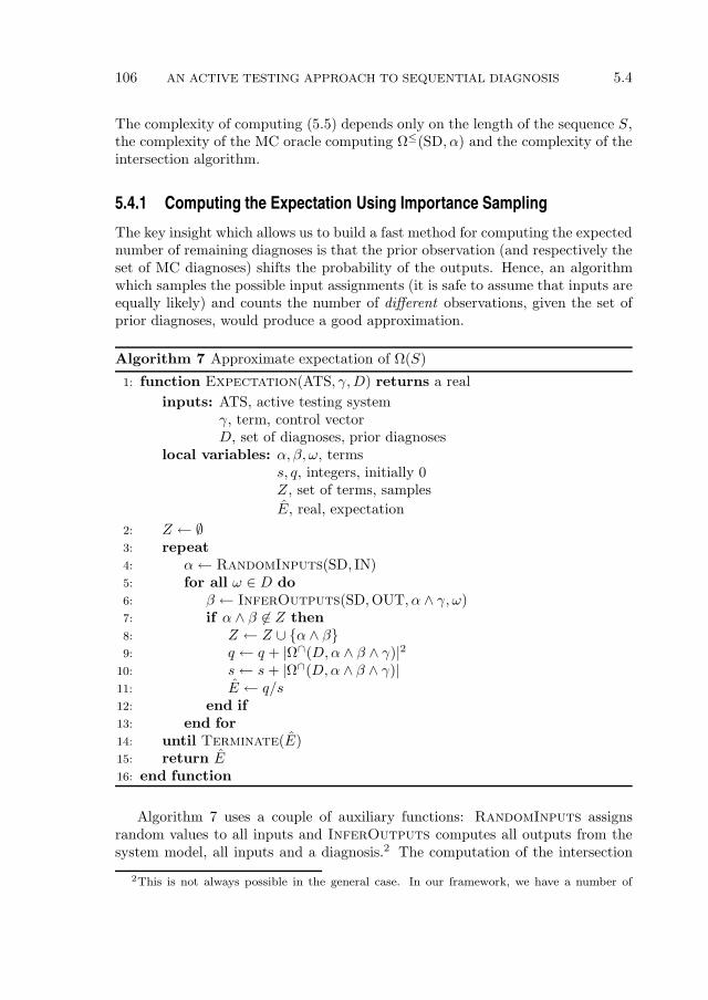
106 AN ACTIVE TESTING APPROACH TO SEQUENTIAL DIAGNOSIS 5.4
The complexity of computing (5.5) depends only on the length of the sequence S,the complexity of the MC oracle computing Ω≤(SD, α) and the complexity of theintersection algorithm.
5.4.1 Computing the Expectation Using Importance Sampling
The key insight which allows us to build a fast method for computing the expectednumber of remaining diagnoses is that the prior observation (and respectively theset of MC diagnoses) shifts the probability of the outputs. Hence, an algorithmwhich samples the possible input assignments (it is safe to assume that inputs areequally likely) and counts the number of different observations, given the set ofprior diagnoses, would produce a good approximation.
Algorithm 7 Approximate expectation of Ω(S)
1: function Expectation(ATS, γ,D) returns a real
inputs: ATS, active testing systemγ, term, control vectorD, set of diagnoses, prior diagnoses
local variables: α, β, ω, termss, q, integers, initially 0Z, set of terms, samples
E, real, expectation
2: Z ← ∅3: repeat
4: α← RandomInputs(SD, IN)5: for all ω ∈ D do
6: β ← InferOutputs(SD,OUT, α ∧ γ, ω)7: if α ∧ β 6∈ Z then
8: Z ← Z ∪ α ∧ β9: q ← q + |Ω∩(D,α ∧ β ∧ γ)|2
10: s← s+ |Ω∩(D,α ∧ β ∧ γ)|11: E ← q/s12: end if
13: end for
14: until Terminate(E)15: return E16: end function
Algorithm 7 uses a couple of auxiliary functions: RandomInputs assignsrandom values to all inputs and InferOutputs computes all outputs from thesystem model, all inputs and a diagnosis.2 The computation of the intersection
2This is not always possible in the general case. In our framework, we have a number of
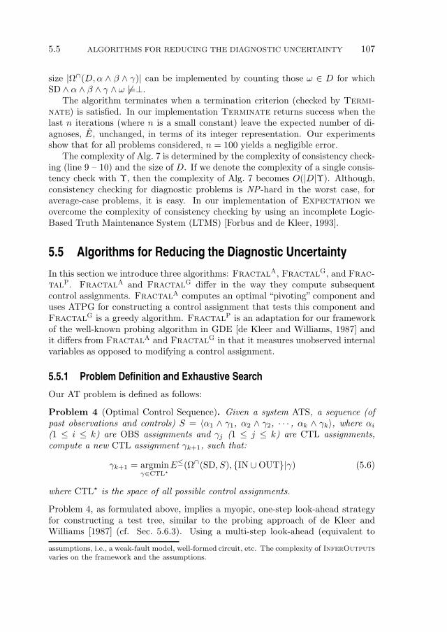
5.5 ALGORITHMS FOR REDUCING THE DIAGNOSTIC UNCERTAINTY 107
size |Ω∩(D,α ∧ β ∧ γ)| can be implemented by counting those ω ∈ D for whichSD ∧ α ∧ β ∧ γ ∧ ω 6|=⊥.
The algorithm terminates when a termination criterion (checked by Termi-
nate) is satisfied. In our implementation Terminate returns success when thelast n iterations (where n is a small constant) leave the expected number of di-agnoses, E, unchanged, in terms of its integer representation. Our experimentsshow that for all problems considered, n = 100 yields a negligible error.
The complexity of Alg. 7 is determined by the complexity of consistency check-ing (line 9 – 10) and the size of D. If we denote the complexity of a single consis-tency check with Υ, then the complexity of Alg. 7 becomes O(|D|Υ). Although,consistency checking for diagnostic problems is NP-hard in the worst case, foraverage-case problems, it is easy. In our implementation of Expectation weovercome the complexity of consistency checking by using an incomplete Logic-Based Truth Maintenance System (LTMS) [Forbus and de Kleer, 1993].
5.5 Algorithms for Reducing the Diagnostic Uncertainty
In this section we introduce three algorithms: FractalA, FractalG, and Frac-
talP. FractalA and FractalG differ in the way they compute subsequentcontrol assignments. FractalA computes an optimal “pivoting” component anduses ATPG for constructing a control assignment that tests this component andFractalG is a greedy algorithm. FractalP is an adaptation for our frameworkof the well-known probing algorithm in GDE [de Kleer and Williams, 1987] andit differs from FractalA and FractalG in that it measures unobserved internalvariables as opposed to modifying a control assignment.
5.5.1 Problem Definition and Exhaustive Search
Our AT problem is defined as follows:
Problem 4 (Optimal Control Sequence). Given a system ATS, a sequence (ofpast observations and controls) S = 〈α1 ∧ γ1, α2 ∧ γ2, · · · , αk ∧ γk〉, where αi
(1 ≤ i ≤ k) are OBS assignments and γj (1 ≤ j ≤ k) are CTL assignments,compute a new CTL assignment γk+1, such that:
γk+1 = argminγ∈CTL⋆
E≤(Ω∩(SD, S), IN ∪OUT|γ) (5.6)
where CTL⋆ is the space of all possible control assignments.
Problem 4, as formulated above, implies a myopic, one-step look-ahead strategyfor constructing a test tree, similar to the probing approach of de Kleer andWilliams [1987] (cf. Sec. 5.6.3). Using a multi-step look-ahead (equivalent to
assumptions, i.e., a weak-fault model, well-formed circuit, etc. The complexity of InferOutputs
varies on the framework and the assumptions.
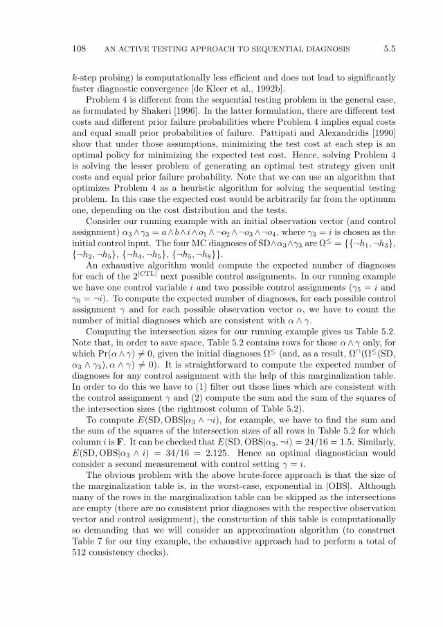
108 AN ACTIVE TESTING APPROACH TO SEQUENTIAL DIAGNOSIS 5.5
k-step probing) is computationally less efficient and does not lead to significantlyfaster diagnostic convergence [de Kleer et al., 1992b].
Problem 4 is different from the sequential testing problem in the general case,as formulated by Shakeri [1996]. In the latter formulation, there are different testcosts and different prior failure probabilities where Problem 4 implies equal costsand equal small prior probabilities of failure. Pattipati and Alexandridis [1990]show that under those assumptions, minimizing the test cost at each step is anoptimal policy for minimizing the expected test cost. Hence, solving Problem 4is solving the lesser problem of generating an optimal test strategy given unitcosts and equal prior failure probability. Note that we can use an algorithm thatoptimizes Problem 4 as a heuristic algorithm for solving the sequential testingproblem. In this case the expected cost would be arbitrarily far from the optimumone, depending on the cost distribution and the tests.
Consider our running example with an initial observation vector (and controlassignment) α3∧γ3 = a∧b∧ i∧o1∧¬o2∧¬o3∧¬o4, where γ3 = i is chosen as theinitial control input. The four MC diagnoses of SD∧α3∧γ3 are Ω≤ = ¬h1,¬h3,¬h2,¬h5, ¬h4,¬h5, ¬h5,¬h8.
An exhaustive algorithm would compute the expected number of diagnosesfor each of the 2|CTL| next possible control assignments. In our running examplewe have one control variable i and two possible control assignments (γ5 = i andγ6 = ¬i). To compute the expected number of diagnoses, for each possible controlassignment γ and for each possible observation vector α, we have to count thenumber of initial diagnoses which are consistent with α ∧ γ.
Computing the intersection sizes for our running example gives us Table 5.2.Note that, in order to save space, Table 5.2 contains rows for those α∧γ only, forwhich Pr(α∧ γ) 6= 0, given the initial diagnoses Ω≤ (and, as a result, Ω∩(Ω≤(SD,α3 ∧ γ3), α ∧ γ) 6= 0). It is straightforward to compute the expected number ofdiagnoses for any control assignment with the help of this marginalization table.In order to do this we have to (1) filter out those lines which are consistent withthe control assignment γ and (2) compute the sum and the sum of the squares ofthe intersection sizes (the rightmost column of Table 5.2).
To compute E(SD,OBS|α3 ∧ ¬i), for example, we have to find the sum andthe sum of the squares of the intersection sizes of all rows in Table 5.2 for whichcolumn i is F. It can be checked that E(SD,OBS|α3,¬i) = 24/16 = 1.5. Similarly,E(SD,OBS|α3 ∧ i) = 34/16 = 2.125. Hence an optimal diagnostician wouldconsider a second measurement with control setting γ = i.
The obvious problem with the above brute-force approach is that the size ofthe marginalization table is, in the worst-case, exponential in |OBS|. Althoughmany of the rows in the marginalization table can be skipped as the intersectionsare empty (there are no consistent prior diagnoses with the respective observationvector and control assignment), the construction of this table is computationallyso demanding that we will consider an approximation algorithm (to constructTable 7 for our tiny example, the exhaustive approach had to perform a total of512 consistency checks).

5.5 ALGORITHMS FOR REDUCING THE DIAGNOSTIC UNCERTAINTY 109
Table 5.2: Marginalization table for SD and α3
i a b o1 o2 o3 o4 Pr |Ω∩| i a b o1 o2 o3 o4 Pr |Ω∩|F F F F F F F 0.03125 1 F T T T F F T 0.03125 1F F F T F F F 0.0625 2 T F F F F F T 0.0625 2F F F T F F T 0.03125 1 T F F F F T F 0.03125 1F F T F F F F 0.03125 1 T F F F T F F 0.03125 1F F T T F F F 0.0625 2 T F T F T F F 0.03125 1F F T T F F T 0.03125 1 T F T T F F F 0.03125 1F T F F F F F 0.03125 1 T F T T F T T 0.0625 2F T F T F F F 0.0625 2 T T F F F T F 0.03125 1F T F T F F T 0.03125 1 T T F T F F F 0.03125 1F T T F F F F 0.03125 1 T T F T T F T 0.0625 2F T T T F F F 0.0625 2 T T T T F F F 0.125 4
5.5.2 FRACTALA
Consider the running example from Sec. 5.3 and an observation α4 = a ∧ b ∧ i ∧o1 ∧ ¬o4. This leads to the 6 double-fault MC diagnoses, shown in Fig. 5.3.
7
7
7
7
7
h8
3
133
h7
7
7
7
7
7
7
6
7
7
7
7
7
h4
3
133
7
7
7
7
7
h2
3
133
7
7
7
7
h3
3
3
103
7
3
h5
3
3
3
3
133
7
7
7
7
h1
3
3
103
7
7
7
7
7
7
h6
6
ω1
ω2
ω3
ω4
ω5
ω6
E≤
Figure 5.3: ATPG-Based active testing example
Instead of searching through the space of all possible control assignments, wedirectly compute a control assignment that tests a specific component c by us-ing an approach from ATPG. We choose this component c to be the one thatmost decreases the expected number of remaining MC diagnoses by minimizingE≤(SD, c|α ∧ γ). If we look at Fig. 5.3 we can see that knowing the health of h1
and h3 leads to E≤ ≈ 3.33, for h2, h4, h5, and h7, we have E≤ ≈ 4.33, and forh6 and h7 we have E≤ = 6. Choosing a control setting that computes the stateof h1 or h3 is intuitive as the state of this component makes the most balancedpartition of the prior diagnoses.

110 AN ACTIVE TESTING APPROACH TO SEQUENTIAL DIAGNOSIS 5.5
We next present the FractalA algorithm that uses the approach illustratedabove.
Algorithm 8 ATPG-Based active testing algorithm
1: function FractalATPG(ATS, α, γ) returns a control term
inputs: ATS, active testing systemα, term, initial (non-modifiable) observationγ, term, initial control
local variables: c, component variablef , integerd, term, diagnosisγ, term, control settingH , set of pairs, component/expectation pairsD, set of terms, diagnoses
2: D ← Ω≤(SD, α ∧ γ)3: for all c ∈ COMPS do
4: f ← 05: for all d ∈ D do
6: if c ∈ d then
7: f ← f + 18: end if
9: end for
10: H ← 〈c, f2 + (|D| − f)2〉11: end for
12: H ← SortByExpectation(H)13: for i = 1 . . . |H | do
14: if γ ← ATPG(ATS, α,Hi〈c〉) then
15: return γ16: end if
17: end for
18: return RandomControls()19: end function
Algorithm 8 counts in how many prior diagnoses each component appears (lines4 - 8) and the result is saved in the variable f . This number is then used tocompute the expected number of remaining MC diagnoses given the componenthealth (line 10). For each component the expected number of diagnoses is storedin the set H (line 10). The set H is then sorted in increasing order of expectation(line 12). We then iterate over the set of components in order of expectation (lines13 – 17). For each component we try to compute an ATPG vector that tests it. Insome cases such vector may not exist. In the worst case there is no ATPG vectorthat can test any component and Alg. 8 has no better strategy but to return arandom control assignment (line 18).
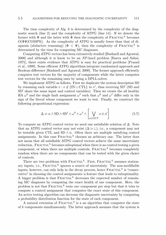
5.5 ALGORITHMS FOR REDUCING THE DIAGNOSTIC UNCERTAINTY 111
The time complexity of Alg. 8 is determined by the complexity of the diag-nostic search (line 2) and the complexity of ATPG (line 14). If we denote theformer with Ψ and the latter with Φ then the complexity of FractalA becomesO(ΦΨ|COMPS|). As the complexity of ATPG is usually lower than that of di-agnosis (abductive reasoning) (Φ < Ψ), then the complexity of FractalA isdetermined by the time for computing MC diagnoses.
Computing ATPG vectors has been extensively studied [Bushnell and Agrawal,2000] and although it is know to be an NP-hard problem [Ibarra and Sahni,1975], there exists evidence that ATPG is easy for practical problems [Prasadet al., 1999]. Some efficient ATPG algorithms integrate randomized approach andBoolean difference [Bushnell and Agrawal, 2000]. The former approach efficientlycomputes test vectors for the majority of components while the latter computestest vectors for the remaining ones by using a DPLL-solver.
We implement ATPG as follows. First we duplicate the system description SDby renaming each variable v : v 6∈ IN ∪ CTL to v′, thus receiving SD′ (SD andSD′ share the same input and control variables). Then we create the all healthyHA ω0 and the single fault assignment ωI such that ω0 and ωI differ only in thesign of the literal whose component we want to test. Finally, we construct thefollowing propositional expression:
∆ ≡ α ∧ SD ∧ SD′ ∧ ω0 ∧ ωI ∧[
∨
o∈OUT
o⊕ o′]
(5.7)
To compute an ATPG control vector we need one satisfiable solution of ∆. Notethat an ATPG control vector may not exist (∆ |=⊥), i.e., a component may notbe testable given CTL and SD ∧ α. Often there are multiple satisfying controlassignments. In this case FractalA chooses an arbitrary one. The latter doesnot mean that all satisfiable ATPG control vectors achieve the same uncertaintyreduction. FractalA becomes suboptimal when there is no control testing a givencomponent, or when there are multiple controls. FractalA becomes completelyrandom when there are no components that can be tested with the given choiceof controls.
There are two problems with FractalA. First, FractalA assumes station-ary inputs, i.e., FractalA ignores a source of uncertainty. The non-modifiableinputs, however, can only help in the decay process, hence FractalA is “conser-vative” in choosing the control assignments–a feature that leads to suboptimality.A bigger problem is that FractalA decreases the expected number of remain-ing MC diagnoses by computing the exact health of one component. Here, theproblem is not that FractalA tests one component per step but that it tries tocompute a control assignment that computes the exact state of this component.An active testing algorithm can decrease the diagnostic uncertainty by computinga probability distribution function for the state of each component.
A natural extension of FractalA is a an algorithm that computes the stateof k components simultaneously. The latter approach assumes that the system is
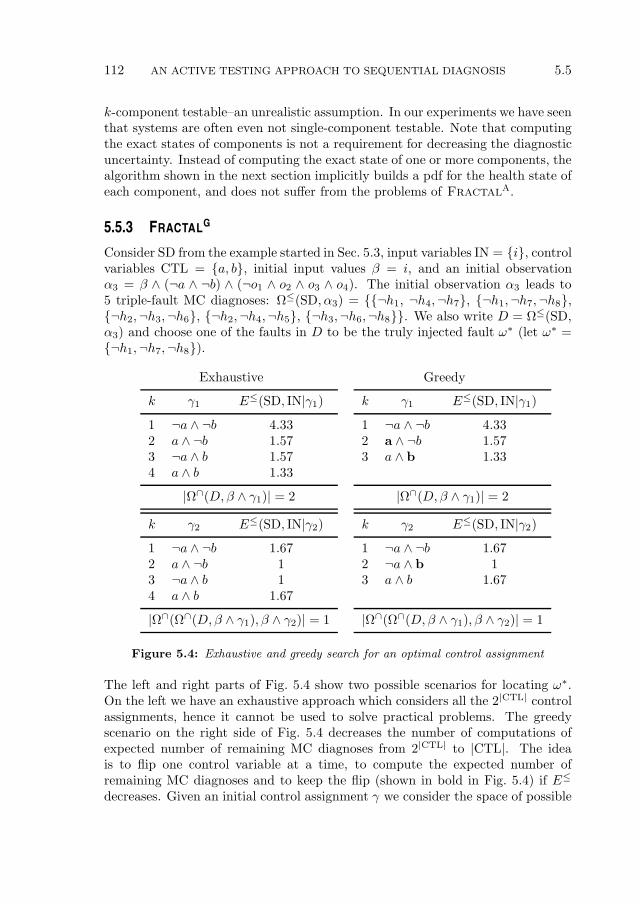
112 AN ACTIVE TESTING APPROACH TO SEQUENTIAL DIAGNOSIS 5.5
k-component testable–an unrealistic assumption. In our experiments we have seenthat systems are often even not single-component testable. Note that computingthe exact states of components is not a requirement for decreasing the diagnosticuncertainty. Instead of computing the exact state of one or more components, thealgorithm shown in the next section implicitly builds a pdf for the health state ofeach component, and does not suffer from the problems of FractalA.
5.5.3 FRACTALG
Consider SD from the example started in Sec. 5.3, input variables IN = i, controlvariables CTL = a, b, initial input values β = i, and an initial observationα3 = β ∧ (¬a ∧ ¬b) ∧ (¬o1 ∧ o2 ∧ o3 ∧ o4). The initial observation α3 leads to5 triple-fault MC diagnoses: Ω≤(SD, α3) = ¬h1, ¬h4,¬h7, ¬h1,¬h7,¬h8,¬h2,¬h3,¬h6, ¬h2,¬h4,¬h5, ¬h3,¬h6,¬h8. We also write D = Ω≤(SD,α3) and choose one of the faults in D to be the truly injected fault ω∗ (let ω∗ =¬h1,¬h7,¬h8).
Exhaustive Greedy
k γ1 E≤(SD, IN|γ1) k γ1 E≤(SD, IN|γ1)
1 ¬a ∧ ¬b 4.33 1 ¬a ∧ ¬b 4.332 a ∧ ¬b 1.57 2 a ∧ ¬b 1.573 ¬a ∧ b 1.57 3 a ∧ b 1.334 a ∧ b 1.33
|Ω∩(D, β ∧ γ1)| = 2 |Ω∩(D, β ∧ γ1)| = 2
k γ2 E≤(SD, IN|γ2) k γ2 E≤(SD, IN|γ2)
1 ¬a ∧ ¬b 1.67 1 ¬a ∧ ¬b 1.672 a ∧ ¬b 1 2 ¬a ∧ b 13 ¬a ∧ b 1 3 a ∧ b 1.674 a ∧ b 1.67
|Ω∩(Ω∩(D, β ∧ γ1), β ∧ γ2)| = 1 |Ω∩(Ω∩(D, β ∧ γ1), β ∧ γ2)| = 1
Figure 5.4: Exhaustive and greedy search for an optimal control assignment
The left and right parts of Fig. 5.4 show two possible scenarios for locating ω∗.On the left we have an exhaustive approach which considers all the 2|CTL| controlassignments, hence it cannot be used to solve practical problems. The greedyscenario on the right side of Fig. 5.4 decreases the number of computations ofexpected number of remaining MC diagnoses from 2|CTL| to |CTL|. The ideais to flip one control variable at a time, to compute the expected number ofremaining MC diagnoses and to keep the flip (shown in bold in Fig. 5.4) if E≤
decreases. Given an initial control assignment γ we consider the space of possible
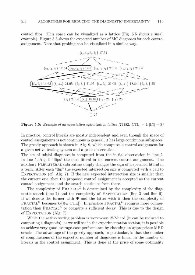
5.5 ALGORITHMS FOR REDUCING THE DIAGNOSTIC UNCERTAINTY 113
control flips. This space can be visualized as a lattice (Fig. 5.5 shows a smallexample). Figure 5.5 shows the expected number of MC diagnoses for each controlassignment. Note that probing can be visualized in a similar way.
i2 21.05 i4 18.84 i6 25 i7 25
25
i2, i4, i6, i7 17.54
i2, i4 14.65 i2, i6 21.05 i2, i7 21.05 i4, i6 21.05 i4, i7 18.84 i6, i7 25
i2, i4, i6 17.54 i2, i4, i7 14.5 i2, i6, i7 21.05 i4, i6, i7 21.05
Figure 5.5: Example of an expectation optimization lattice (74182, |CTL| = 4, |IN| = 5)
In practice, control literals are mostly independent and even though the space ofcontrol assignments is not continuous in general, it has large continuous subspaces.The greedy approach is shown in Alg. 9, which computes a control assignment fora given active testing system and a prior observation.
The set of initial diagnoses is computed from the initial observation in line 2.In line 5, Alg. 9 “flips” the next literal in the current control assignment. Theauxiliary FlipLiteral subroutine simply changes the sign of a specified literal ina term. After each “flip” the expected intersection size is computed with a call toExpectation (cf. Alg. 7). If the new expected intersection size is smaller thanthe current one, then the proposed control assignment is accepted as the currentcontrol assignment, and the search continues from there.
The complexity of FractalG is determined by the complexity of the diag-nostic search (line 2) and the complexity of Expectation (line 3 and line 6).If we denote the former with Ψ and the latter with Ξ then the complexity ofFractalG becomes O(ΦΞ|CTL|). In practice FractalG requires more compu-tation than FractalA to compute a sufficient decay. This is due to the designof Expectation (Alg. 7).
While the active-testing problem is worst-case NP -hard (it can be reduced tocomputing a diagnosis), as we will see in the experimentation section, it is possibleto achieve very good average-case performance by choosing an appropriate MBDoracle. The advantage of the greedy approach, in particular, is that the numberof computations of the expected number of diagnoses is linear in the number ofliterals in the control assignment. This is done at the price of some optimality
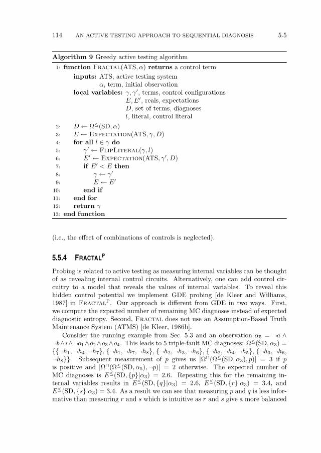
114 AN ACTIVE TESTING APPROACH TO SEQUENTIAL DIAGNOSIS 5.5
Algorithm 9 Greedy active testing algorithm
1: function Fractal(ATS, α) returns a control term
inputs: ATS, active testing systemα, term, initial observation
local variables: γ, γ′, terms, control configurationsE,E′, reals, expectationsD, set of terms, diagnosesl, literal, control literal
2: D ← Ω≤(SD, α)3: E ← Expectation(ATS, γ,D)4: for all l ∈ γ do
5: γ′ ← FlipLiteral(γ, l)6: E′ ← Expectation(ATS, γ′, D)7: if E′ < E then
8: γ ← γ′
9: E ← E′
10: end if
11: end for
12: return γ13: end function
(i.e., the effect of combinations of controls is neglected).
5.5.4 FRACTALP
Probing is related to active testing as measuring internal variables can be thoughtof as revealing internal control circuits. Alternatively, one can add control cir-cuitry to a model that reveals the values of internal variables. To reveal thishidden control potential we implement GDE probing [de Kleer and Williams,1987] in FractalP. Our approach is different from GDE in two ways. First,we compute the expected number of remaining MC diagnoses instead of expecteddiagnostic entropy. Second, Fractal does not use an Assumption-Based TruthMaintenance System (ATMS) [de Kleer, 1986b].
Consider the running example from Sec. 5.3 and an observation α5 = ¬a ∧¬b∧ i∧¬o1∧o2∧o3∧o4. This leads to 5 triple-fault MC diagnoses: Ω≤(SD, α3) =¬h1, ¬h4,¬h7, ¬h1,¬h7,¬h8, ¬h2,¬h3,¬h6, ¬h2,¬h4,¬h5, ¬h3,¬h6,¬h8. Subsequent measurement of p gives us |Ω∩(Ω≤(SD, α3), p)| = 3 if pis positive and |Ω∩(Ω≤(SD, α5),¬p)| = 2 otherwise. The expected number ofMC diagnoses is E≤(SD, p|α3) = 2.6. Repeating this for the remaining in-ternal variables results in E≤(SD, q|α3) = 2.6, E≤(SD, r|α3) = 3.4, andE≤(SD, s|α3) = 3.4. As a result we can see that measuring p and q is less infor-mative than measuring r and s which is intuitive as r and s give a more balanced
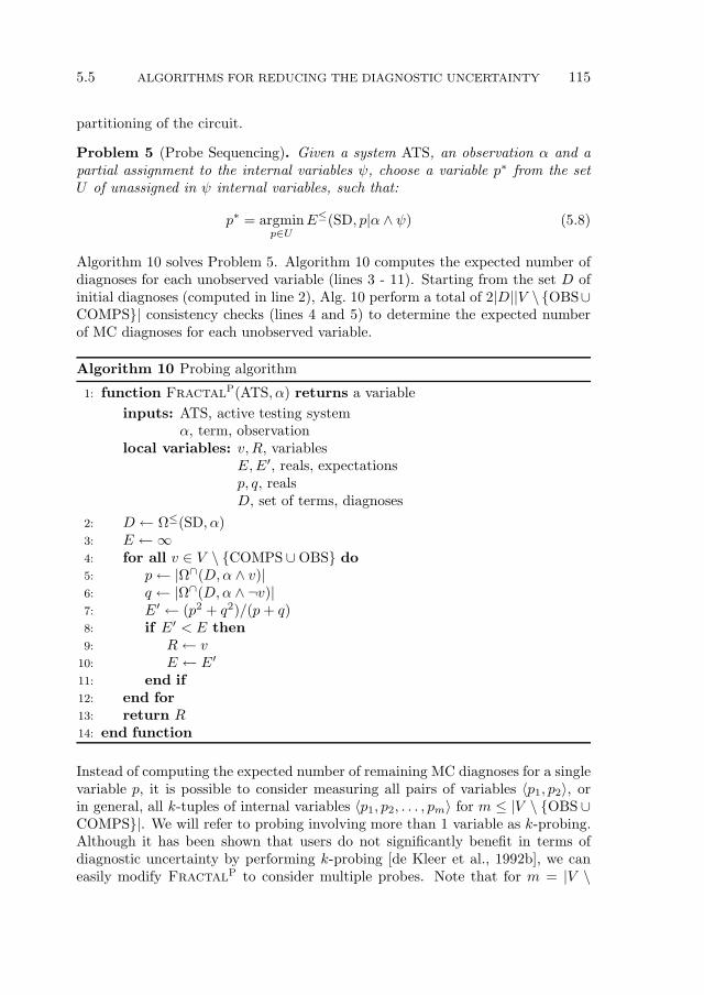
5.5 ALGORITHMS FOR REDUCING THE DIAGNOSTIC UNCERTAINTY 115
partitioning of the circuit.
Problem 5 (Probe Sequencing). Given a system ATS, an observation α and apartial assignment to the internal variables ψ, choose a variable p∗ from the setU of unassigned in ψ internal variables, such that:
p∗ = argminp∈U
E≤(SD, p|α ∧ ψ) (5.8)
Algorithm 10 solves Problem 5. Algorithm 10 computes the expected number ofdiagnoses for each unobserved variable (lines 3 - 11). Starting from the set D ofinitial diagnoses (computed in line 2), Alg. 10 perform a total of 2|D||V \ OBS∪COMPS| consistency checks (lines 4 and 5) to determine the expected numberof MC diagnoses for each unobserved variable.
Algorithm 10 Probing algorithm
1: function FractalP(ATS, α) returns a variable
inputs: ATS, active testing systemα, term, observation
local variables: v,R, variablesE,E′, reals, expectationsp, q, realsD, set of terms, diagnoses
2: D ← Ω≤(SD, α)3: E ←∞4: for all v ∈ V \ COMPS ∪OBS do
5: p← |Ω∩(D,α ∧ v)|6: q ← |Ω∩(D,α ∧ ¬v)|7: E′ ← (p2 + q2)/(p+ q)8: if E′ < E then
9: R← v10: E ← E′
11: end if
12: end for
13: return R14: end function
Instead of computing the expected number of remaining MC diagnoses for a singlevariable p, it is possible to consider measuring all pairs of variables 〈p1, p2〉, orin general, all k-tuples of internal variables 〈p1, p2, . . . , pm〉 for m ≤ |V \ OBS ∪COMPS|. We will refer to probing involving more than 1 variable as k-probing.Although it has been shown that users do not significantly benefit in terms ofdiagnostic uncertainty by performing k-probing [de Kleer et al., 1992b], we caneasily modify FractalP to consider multiple probes. Note that for m = |V \
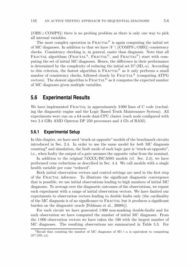
116 AN ACTIVE TESTING APPROACH TO SEQUENTIAL DIAGNOSIS 5.6
OBS ∪ COMPS| there is no probing problem as there is only one way to pickall internal variables.
The most complex operation in FractalP is again computing the initial setof MC diagnoses. In addition to that we have |V \ COMPS∪OBS| consistencychecks. Consistency checking is, in general, easier than diagnosis. Note that allFractal algorithms (FractalA, FractalG, and FractalP) start with com-puting the set of initial MC diagnoses. Hence, the difference in their performanceis determined by the complexity of reducing the initial set Ω≤(SD, α). Accordingto this criterion, the fastest algorithm is FractalP as it only performs a smallnumber of consistency checks, followed closely by FractalA (computing ATPGvectors). The slowest algorithm is FractalG as it computes the expected numberof MC diagnoses given multiple variables.
5.6 Experimental Results
We have implemented Fractal in approximately 3 000 lines of C code (exclud-ing the diagnostic engine and the Logic Based Truth Maintenance System). Allexperiments were run on a 64-node dual-CPU cluster (each node configured withtwo 2.4 GHz AMD Opteron DP 250 processors and 4 Gb of RAM).
5.6.1 Experimental Setup
In this chapter, we have used“stuck-at-opposite”models of the benchmark circuitsintroduced in Sec. 2.4. In order to use the same model for both MC diagnosiscounting3 and simulation, the fault mode of each logic gate is “stuck-at-opposite”,i.e., when faulty the output of a gate assumes the opposite value from the nominal.
In addition to the original 74XXX/ISCAS85 models (cf. Sec. 2.4), we haveperformed cone reductions as described in Sec. 4.4. We call models with a singlehealth variable per cone “reduced”.
Both initial observation vectors and control settings are used in the first stepof the Fractal inference. To illustrate the significant diagnostic convergencethat is possible, we use initial observations leading to high numbers of initial MCdiagnoses. To average over the diagnostic outcomes of the observations, we repeateach experiment with a range of initial observation vectors. We have limited ourexperiments to observation vectors leading to double faults only (the cardinalityof the MC diagnosis is of no significance to Fractal but it produces a significantburden on the diagnostic oracle [Feldman et al., 2008b]).
For each circuit we have generated 1 000 non-masking double-faults and foreach observation we have computed the number of initial MC diagnoses. Fromthe 1 000 observation vectors we have taken the 100 with the largest number ofMC diagnoses. The resulting observations are summarized in Table 5.3. For
3Recall that counting the number of MC diagnoses of SD ∧ α is equivalent to computing|Ω≤(SD, α)|.
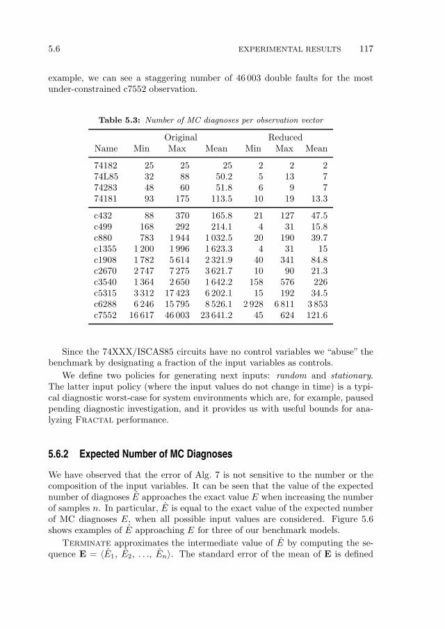
5.6 EXPERIMENTAL RESULTS 117
example, we can see a staggering number of 46 003 double faults for the mostunder-constrained c7552 observation.
Table 5.3: Number of MC diagnoses per observation vector
Original ReducedName Min Max Mean Min Max Mean
74182 25 25 25 2 2 274L85 32 88 50.2 5 13 774283 48 60 51.8 6 9 774181 93 175 113.5 10 19 13.3
c432 88 370 165.8 21 127 47.5c499 168 292 214.1 4 31 15.8c880 783 1 944 1 032.5 20 190 39.7c1355 1 200 1 996 1 623.3 4 31 15c1908 1 782 5 614 2 321.9 40 341 84.8c2670 2 747 7 275 3 621.7 10 90 21.3c3540 1 364 2 650 1 642.2 158 576 226c5315 3 312 17 423 6 202.1 15 192 34.5c6288 6 246 15 795 8 526.1 2 928 6 811 3 853c7552 16 617 46 003 23 641.2 45 624 121.6
Since the 74XXX/ISCAS85 circuits have no control variables we “abuse” thebenchmark by designating a fraction of the input variables as controls.
We define two policies for generating next inputs: random and stationary.The latter input policy (where the input values do not change in time) is a typi-cal diagnostic worst-case for system environments which are, for example, pausedpending diagnostic investigation, and it provides us with useful bounds for ana-lyzing Fractal performance.
5.6.2 Expected Number of MC Diagnoses
We have observed that the error of Alg. 7 is not sensitive to the number or thecomposition of the input variables. It can be seen that the value of the expectednumber of diagnoses E approaches the exact value E when increasing the numberof samples n. In particular, E is equal to the exact value of the expected numberof MC diagnoses E, when all possible input values are considered. Figure 5.6shows examples of E approaching E for three of our benchmark models.
Terminate approximates the intermediate value of E by computing the se-quence E = 〈E1, E2, . . ., En〉. The standard error of the mean of E is defined
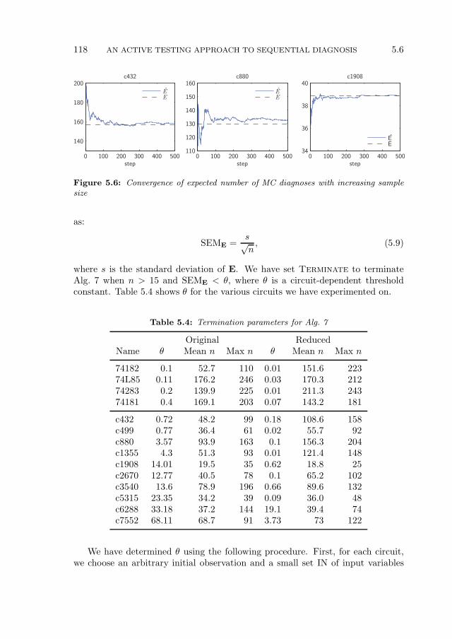
118 AN ACTIVE TESTING APPROACH TO SEQUENTIAL DIAGNOSIS 5.6
0 100 200 300 400 500
140
160
180
200c432
step0 100 200 300 400 500
110
120
130
140
150
160c880
step0 100 200 300 400 500
34
36
38
40c1908
step
ÊE
ÊE
EE
Figure 5.6: Convergence of expected number of MC diagnoses with increasing samplesize
as:
SEME =s√n, (5.9)
where s is the standard deviation of E. We have set Terminate to terminateAlg. 7 when n > 15 and SEME < θ, where θ is a circuit-dependent thresholdconstant. Table 5.4 shows θ for the various circuits we have experimented on.
Table 5.4: Termination parameters for Alg. 7
Original ReducedName θ Mean n Max n θ Mean n Max n
74182 0.1 52.7 110 0.01 151.6 22374L85 0.11 176.2 246 0.03 170.3 21274283 0.2 139.9 225 0.01 211.3 24374181 0.4 169.1 203 0.07 143.2 181
c432 0.72 48.2 99 0.18 108.6 158c499 0.77 36.4 61 0.02 55.7 92c880 3.57 93.9 163 0.1 156.3 204c1355 4.3 51.3 93 0.01 121.4 148c1908 14.01 19.5 35 0.62 18.8 25c2670 12.77 40.5 78 0.1 65.2 102c3540 13.6 78.9 196 0.66 89.6 132c5315 23.35 34.2 39 0.09 36.0 48c6288 33.18 37.2 144 19.1 39.4 74c7552 68.11 68.7 91 3.73 73 122
We have determined θ using the following procedure. First, for each circuit,we choose an arbitrary initial observation and a small set IN of input variables
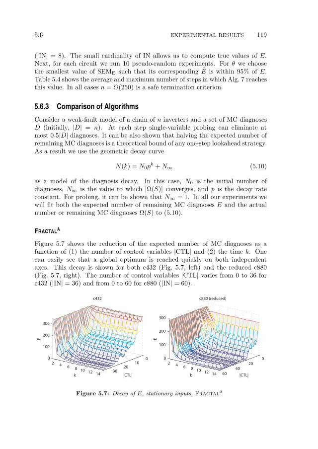
5.6 EXPERIMENTAL RESULTS 119
(|IN| = 8). The small cardinality of IN allows us to compute true values of E.Next, for each circuit we run 10 pseudo-random experiments. For θ we choosethe smallest value of SEME such that its corresponding E is within 95% of E.Table 5.4 shows the average and maximum number of steps in which Alg. 7 reachesthis value. In all cases n = O(250) is a safe termination criterion.
5.6.3 Comparison of Algorithms
Consider a weak-fault model of a chain of n inverters and a set of MC diagnosesD (initially, |D| = n). At each step single-variable probing can eliminate atmost 0.5|D| diagnoses. It can be also shown that halving the expected number ofremaining MC diagnoses is a theoretical bound of any one-step lookahead strategy.As a result we use the geometric decay curve
N(k) = N0pk +N∞ (5.10)
as a model of the diagnosis decay. In this case, N0 is the initial number ofdiagnoses, N∞ is the value to which |Ω(S)| converges, and p is the decay rateconstant. For probing, it can be shown that N∞ = 1. In all our experiments wewill fit both the expected number of remaining MC diagnoses E and the actualnumber or remaining MC diagnoses Ω(S) to (5.10).
FRACTALA
Figure 5.7 shows the reduction of the expected number of MC diagnoses as afunction of (1) the number of control variables |CTL| and (2) the time k. Onecan easily see that a global optimum is reached quickly on both independentaxes. This decay is shown for both c432 (Fig. 5.7, left) and the reduced c880(Fig. 5.7, right). The number of control variables |CTL| varies from 0 to 36 forc432 (|IN| = 36) and from 0 to 60 for c880 (|IN| = 60).
2 4 6 8 10 12 14 6040
2000
100
200
300
|CTL|
c880 (reduced)
k
E
2 4 6 8 10 12 1430
2010
00
100
200
300
|CTL|
c432
k
E
Figure 5.7: Decay of E, stationary inputs, FractalA
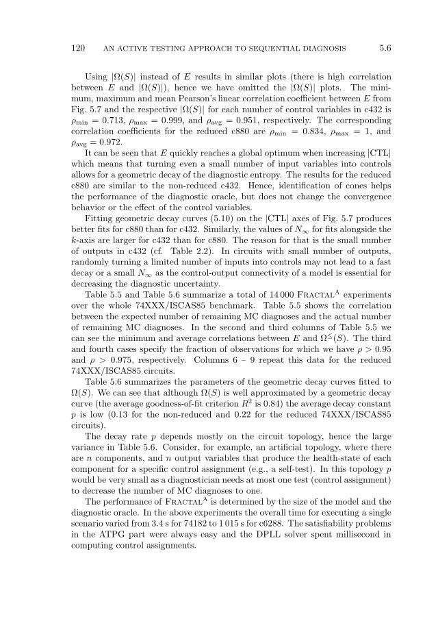
120 AN ACTIVE TESTING APPROACH TO SEQUENTIAL DIAGNOSIS 5.6
Using |Ω(S)| instead of E results in similar plots (there is high correlationbetween E and |Ω(S)|), hence we have omitted the |Ω(S)| plots. The mini-mum, maximum and mean Pearson’s linear correlation coefficient between E fromFig. 5.7 and the respective |Ω(S)| for each number of control variables in c432 isρmin = 0.713, ρmax = 0.999, and ρavg = 0.951, respectively. The correspondingcorrelation coefficients for the reduced c880 are ρmin = 0.834, ρmax = 1, andρavg = 0.972.
It can be seen that E quickly reaches a global optimum when increasing |CTL|which means that turning even a small number of input variables into controlsallows for a geometric decay of the diagnostic entropy. The results for the reducedc880 are similar to the non-reduced c432. Hence, identification of cones helpsthe performance of the diagnostic oracle, but does not change the convergencebehavior or the effect of the control variables.
Fitting geometric decay curves (5.10) on the |CTL| axes of Fig. 5.7 producesbetter fits for c880 than for c432. Similarly, the values of N∞ for fits alongside thek-axis are larger for c432 than for c880. The reason for that is the small numberof outputs in c432 (cf. Table 2.2). In circuits with small number of outputs,randomly turning a limited number of inputs into controls may not lead to a fastdecay or a small N∞ as the control-output connectivity of a model is essential fordecreasing the diagnostic uncertainty.
Table 5.5 and Table 5.6 summarize a total of 14 000 FractalA experimentsover the whole 74XXX/ISCAS85 benchmark. Table 5.5 shows the correlationbetween the expected number of remaining MC diagnoses and the actual numberof remaining MC diagnoses. In the second and third columns of Table 5.5 wecan see the minimum and average correlations between E and Ω≤(S). The thirdand fourth cases specify the fraction of observations for which we have ρ > 0.95and ρ > 0.975, respectively. Columns 6 – 9 repeat this data for the reduced74XXX/ISCAS85 circuits.
Table 5.6 summarizes the parameters of the geometric decay curves fitted toΩ(S). We can see that although Ω(S) is well approximated by a geometric decaycurve (the average goodness-of-fit criterion R2 is 0.84) the average decay constantp is low (0.13 for the non-reduced and 0.22 for the reduced 74XXX/ISCAS85circuits).
The decay rate p depends mostly on the circuit topology, hence the largevariance in Table 5.6. Consider, for example, an artificial topology, where thereare n components, and n output variables that produce the health-state of eachcomponent for a specific control assignment (e.g., a self-test). In this topology pwould be very small as a diagnostician needs at most one test (control assignment)to decrease the number of MC diagnoses to one.
The performance of FractalA is determined by the size of the model and thediagnostic oracle. In the above experiments the overall time for executing a singlescenario varied from 3.4 s for 74182 to 1 015 s for c6288. The satisfiability problemsin the ATPG part were always easy and the DPLL solver spent millisecond incomputing control assignments.
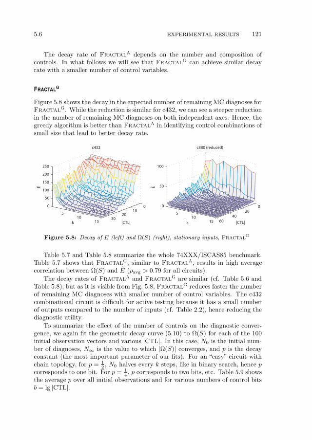
5.6 EXPERIMENTAL RESULTS 121
The decay rate of FractalA depends on the number and composition ofcontrols. In what follows we will see that FractalG can achieve similar decayrate with a smaller number of control variables.
FRACTALG
Figure 5.8 shows the decay in the expected number of remaining MC diagnoses forFractalG. While the reduction is similar for c432, we can see a steeper reductionin the number of remaining MC diagnoses on both independent axes. Hence, thegreedy algorithm is better than FractalA in identifying control combinations ofsmall size that lead to better decay rate.
510
1530
2010
00
50
100
150
200
250
|CTL|
c432
k
^ E
510
15 6040
2000
50
100
|CTL|
c880 (reduced)
k
^ E
Figure 5.8: Decay of E (left) and Ω(S) (right), stationary inputs, FractalG
Table 5.7 and Table 5.8 summarize the whole 74XXX/ISCAS85 benchmark.Table 5.7 shows that FractalG, similar to FractalA, results in high averagecorrelation between Ω(S) and E (ρavg > 0.79 for all circuits).
The decay rates of FractalA and FractalG are similar (cf. Table 5.6 andTable 5.8), but as it is visible from Fig. 5.8, FractalG reduces faster the numberof remaining MC diagnoses with smaller number of control variables. The c432combinational circuit is difficult for active testing because it has a small numberof outputs compared to the number of inputs (cf. Table 2.2), hence reducing thediagnostic utility.
To summarize the effect of the number of controls on the diagnostic conver-gence, we again fit the geometric decay curve (5.10) to Ω(S) for each of the 100initial observation vectors and various |CTL|. In this case, N0 is the initial num-ber of diagnoses, N∞ is the value to which |Ω(S)| converges, and p is the decayconstant (the most important parameter of our fits). For an “easy” circuit withchain topology, for p = 1
2 , N0 halves every k steps, like in binary search, hence pcorresponds to one bit. For p = 1
4 , p corresponds to two bits, etc. Table 5.9 showsthe average p over all initial observations and for various numbers of control bitsb = lg |CTL|.
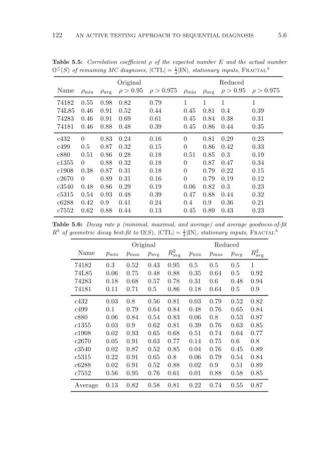
122 AN ACTIVE TESTING APPROACH TO SEQUENTIAL DIAGNOSIS 5.6
Table 5.5: Correlation coefficient ρ of the expected number E and the actual number
Ω≤(S) of remaining MC diagnoses, |CTL| = 14|IN|, stationary inputs, FractalA
Original ReducedName ρmin ρavg ρ > 0.95 ρ > 0.975 ρmin ρavg ρ > 0.95 ρ > 0.975
74182 0.55 0.98 0.82 0.79 1 1 1 174L85 0.46 0.91 0.52 0.44 0.45 0.81 0.4 0.3974283 0.46 0.91 0.69 0.61 0.45 0.84 0.38 0.3174181 0.46 0.88 0.48 0.39 0.45 0.86 0.44 0.35
c432 0 0.83 0.24 0.16 0 0.81 0.29 0.23c499 0.5 0.87 0.32 0.15 0 0.86 0.42 0.33c880 0.51 0.86 0.28 0.18 0.51 0.85 0.3 0.19c1355 0 0.88 0.32 0.18 0 0.87 0.47 0.34c1908 0.38 0.87 0.31 0.18 0 0.79 0.22 0.15c2670 0 0.89 0.31 0.16 0 0.79 0.19 0.12c3540 0.48 0.86 0.29 0.19 0.06 0.82 0.3 0.23c5315 0.54 0.93 0.48 0.39 0.47 0.88 0.44 0.32c6288 0.42 0.9 0.41 0.24 0.4 0.9 0.36 0.21c7552 0.62 0.88 0.44 0.13 0.45 0.89 0.43 0.23
Table 5.6: Decay rate p (minimal, maximal, and average) and average goodness-of-fit
R2 of geometric decay best-fit to Ω(S), |CTL| = 14|IN|, stationary inputs, FractalA
Original ReducedName pmin pmax pavg R2
avg pmin pmax pavg R2avg
74182 0.3 0.52 0.43 0.95 0.5 0.5 0.5 174L85 0.06 0.75 0.48 0.88 0.35 0.64 0.5 0.9274283 0.18 0.68 0.57 0.78 0.31 0.6 0.48 0.9474181 0.11 0.71 0.5 0.86 0.18 0.64 0.5 0.9
c432 0.03 0.8 0.56 0.81 0.03 0.79 0.52 0.82c499 0.1 0.79 0.64 0.84 0.48 0.76 0.65 0.84c880 0.06 0.84 0.54 0.83 0.06 0.8 0.53 0.87c1355 0.03 0.9 0.62 0.81 0.39 0.76 0.63 0.85c1908 0.02 0.93 0.65 0.68 0.51 0.74 0.64 0.77c2670 0.05 0.91 0.63 0.77 0.14 0.75 0.6 0.8c3540 0.02 0.87 0.52 0.85 0.04 0.76 0.45 0.89c5315 0.22 0.91 0.65 0.8 0.06 0.79 0.54 0.84c6288 0.02 0.91 0.52 0.88 0.02 0.9 0.51 0.89c7552 0.56 0.95 0.76 0.61 0.01 0.88 0.58 0.85
Average 0.13 0.82 0.58 0.81 0.22 0.74 0.55 0.87
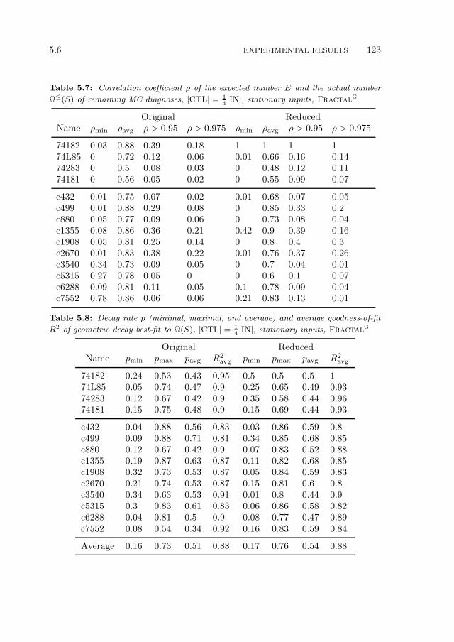
5.6 EXPERIMENTAL RESULTS 123
Table 5.7: Correlation coefficient ρ of the expected number E and the actual number
Ω≤(S) of remaining MC diagnoses, |CTL| = 14|IN|, stationary inputs, FractalG
Original ReducedName ρmin ρavg ρ > 0.95 ρ > 0.975 ρmin ρavg ρ > 0.95 ρ > 0.975
74182 0.03 0.88 0.39 0.18 1 1 1 174L85 0 0.72 0.12 0.06 0.01 0.66 0.16 0.1474283 0 0.5 0.08 0.03 0 0.48 0.12 0.1174181 0 0.56 0.05 0.02 0 0.55 0.09 0.07
c432 0.01 0.75 0.07 0.02 0.01 0.68 0.07 0.05c499 0.01 0.88 0.29 0.08 0 0.85 0.33 0.2c880 0.05 0.77 0.09 0.06 0 0.73 0.08 0.04c1355 0.08 0.86 0.36 0.21 0.42 0.9 0.39 0.16c1908 0.05 0.81 0.25 0.14 0 0.8 0.4 0.3c2670 0.01 0.83 0.38 0.22 0.01 0.76 0.37 0.26c3540 0.34 0.73 0.09 0.05 0 0.7 0.04 0.01c5315 0.27 0.78 0.05 0 0 0.6 0.1 0.07c6288 0.09 0.81 0.11 0.05 0.1 0.78 0.09 0.04c7552 0.78 0.86 0.06 0.06 0.21 0.83 0.13 0.01
Table 5.8: Decay rate p (minimal, maximal, and average) and average goodness-of-fit
R2 of geometric decay best-fit to Ω(S), |CTL| = 14|IN|, stationary inputs, FractalG
Original ReducedName pmin pmax pavg R2
avg pmin pmax pavg R2avg
74182 0.24 0.53 0.43 0.95 0.5 0.5 0.5 174L85 0.05 0.74 0.47 0.9 0.25 0.65 0.49 0.9374283 0.12 0.67 0.42 0.9 0.35 0.58 0.44 0.9674181 0.15 0.75 0.48 0.9 0.15 0.69 0.44 0.93
c432 0.04 0.88 0.56 0.83 0.03 0.86 0.59 0.8c499 0.09 0.88 0.71 0.81 0.34 0.85 0.68 0.85c880 0.12 0.67 0.42 0.9 0.07 0.83 0.52 0.88c1355 0.19 0.87 0.63 0.87 0.11 0.82 0.68 0.85c1908 0.32 0.73 0.53 0.87 0.05 0.84 0.59 0.83c2670 0.21 0.74 0.53 0.87 0.15 0.81 0.6 0.8c3540 0.34 0.63 0.53 0.91 0.01 0.8 0.44 0.9c5315 0.3 0.83 0.61 0.83 0.06 0.86 0.58 0.82c6288 0.04 0.81 0.5 0.9 0.08 0.77 0.47 0.89c7552 0.08 0.54 0.34 0.92 0.16 0.83 0.59 0.84
Average 0.16 0.73 0.51 0.88 0.17 0.76 0.54 0.88
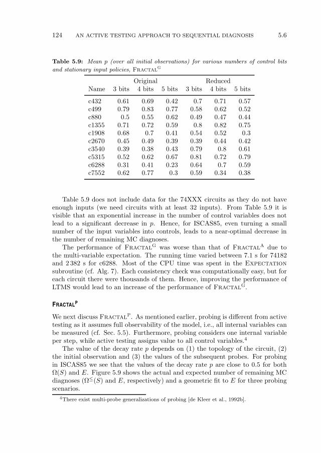
124 AN ACTIVE TESTING APPROACH TO SEQUENTIAL DIAGNOSIS 5.6
Table 5.9: Mean p (over all initial observations) for various numbers of control bits
and stationary input policies, FractalG
Original ReducedName 3 bits 4 bits 5 bits 3 bits 4 bits 5 bits
c432 0.61 0.69 0.42 0.7 0.71 0.57c499 0.79 0.83 0.77 0.58 0.62 0.52c880 0.5 0.55 0.62 0.49 0.47 0.44c1355 0.71 0.72 0.59 0.8 0.82 0.75c1908 0.68 0.7 0.41 0.54 0.52 0.3c2670 0.45 0.49 0.39 0.39 0.44 0.42c3540 0.39 0.38 0.43 0.79 0.8 0.61c5315 0.52 0.62 0.67 0.81 0.72 0.79c6288 0.31 0.41 0.23 0.64 0.7 0.59c7552 0.62 0.77 0.3 0.59 0.34 0.38
Table 5.9 does not include data for the 74XXX circuits as they do not haveenough inputs (we need circuits with at least 32 inputs). From Table 5.9 it isvisible that an exponential increase in the number of control variables does notlead to a significant decrease in p. Hence, for ISCAS85, even turning a smallnumber of the input variables into controls, leads to a near-optimal decrease inthe number of remaining MC diagnoses.
The performance of FractalG was worse than that of FractalA due tothe multi-variable expectation. The running time varied between 7.1 s for 74182and 2 382 s for c6288. Most of the CPU time was spent in the Expectation
subroutine (cf. Alg. 7). Each consistency check was computationally easy, but foreach circuit there were thousands of them. Hence, improving the performance ofLTMS would lead to an increase of the performance of FractalG.
FRACTALP
We next discuss FractalP. As mentioned earlier, probing is different from activetesting as it assumes full observability of the model, i.e., all internal variables canbe measured (cf. Sec. 5.5). Furthermore, probing considers one internal variableper step, while active testing assigns value to all control variables.4
The value of the decay rate p depends on (1) the topology of the circuit, (2)the initial observation and (3) the values of the subsequent probes. For probingin ISCAS85 we see that the values of the decay rate p are close to 0.5 for bothΩ(S) and E. Figure 5.9 shows the actual and expected number of remaining MCdiagnoses (Ω≤(S) and E, respectively) and a geometric fit to E for three probingscenarios.
4There exist multi-probe generalizations of probing [de Kleer et al., 1992b].
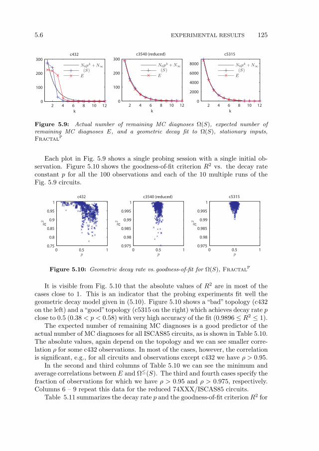
5.6 EXPERIMENTAL RESULTS 125
2 4 6 8 10 120
100
200
300
k
c432
N0pk + N∞
(S)
E
2 4 6 8 10 120
100
200
300
k
c3540 (reduced)
N0pk + N∞
(S)
E
2 4 6 8 10 120
2000
4000
6000
8000
k
c5315
N0pk + N∞
(S)E
Figure 5.9: Actual number of remaining MC diagnoses Ω(S), expected number ofremaining MC diagnoses E, and a geometric decay fit to Ω(S), stationary inputs,FractalP
Each plot in Fig. 5.9 shows a single probing session with a single initial ob-servation. Figure 5.10 shows the goodness-of-fit criterion R2 vs. the decay rateconstant p for all the 100 observations and each of the 10 multiple runs of theFig. 5.9 circuits.
0 0.5 10.75
0.8
0.85
0.9
0.95
1
p
R2
c432
0 0.5 10.975
0.98
0.985
0.99
0.995
1
p
R2
c5315
0 0.5 10.975
0.98
0.985
0.99
0.995
1
p
R2
c3540 (reduced)
Figure 5.10: Geometric decay rate vs. goodness-of-fit for Ω(S), FractalP
It is visible from Fig. 5.10 that the absolute values of R2 are in most of thecases close to 1. This is an indicator that the probing experiments fit well thegeometric decay model given in (5.10). Figure 5.10 shows a “bad” topology (c432on the left) and a“good”topology (c5315 on the right) which achieves decay rate pclose to 0.5 (0.38 < p < 0.58) with very high accuracy of the fit (0.9896 ≤ R2 ≤ 1).
The expected number of remaining MC diagnoses is a good predictor of theactual number of MC diagnoses for all ISCAS85 circuits, as is shown in Table 5.10.The absolute values, again depend on the topology and we can see smaller corre-lation ρ for some c432 observations. In most of the cases, however, the correlationis significant, e.g., for all circuits and observations except c432 we have ρ > 0.95.
In the second and third columns of Table 5.10 we can see the minimum andaverage correlations between E and Ω≤(S). The third and fourth cases specify thefraction of observations for which we have ρ > 0.95 and ρ > 0.975, respectively.Columns 6 – 9 repeat this data for the reduced 74XXX/ISCAS85 circuits.
Table 5.11 summarizes the decay rate p and the goodness-of-fit criterionR2 for
126 AN ACTIVE TESTING APPROACH TO SEQUENTIAL DIAGNOSIS 5.6
all observations and circuits. For c432, the values of p and R2 are more dispersed,while in the other experiments p strongly resembles that of “chained-elements”(i.e., p is close to 0.5). The minimum, maximum and average values of p (percircuit) are given in columns pmin, pmax, and pavg, respectively.
5.6.4 Experimental Summary
If we compare Table 5.5 and Table 5.10 we can see that the average correlationρavg decreases significantly. Hence assuming limited observability (assuming thatnot all internals are measurable) decreases the quality of E as a predictor ofΩ(S). The increased statistical dispersion of ρ is visible from the increased rangeρmax − ρmin (cf. Table 5.5, ρmax is always 1). For example, if we consider c2670,the standard deviation of all E vs. Ω(S) correlation coefficients ρ is σρ = 0.0031for FractalP and σρ = 0.0783 for FractalA. The difference in dispersion ofcorrelation coefficients is significant for all circuits, with smallest values for c432,where it is 0.0038 for FractalP and 0.0825 for FractalA.
By comparing Table 5.6, Table 5.8, and Table 5.11 we can see that the meandecay rates of FractalA, FractalG, and FractalP are similar (the average p ofFractalG is 0.7 while the average p of FractalA is 0.73). The average goodness-of-fit criterion R2 for exponential decays is always good (0.88 for FractalG, 0.84for FractalA), and almost perfect in probing (0.97).
The summary of our experiments is best shown in Fig. 5.11. To factor outsampling error and to be able to perform exhaustive computations we have chosenthe smallest 74182 circuit. The original 74182 (a 4-bit carry-lookahead generator)has 19 components, 9 inputs, and 5 outputs. We have turned 4 of the inputs intocontrols (hence, |IN| = 4 and |CTL| = 4).
We have considered a random control policy in addition to FractalP, Frac-
talA, and FractalG. With random control policy, at each step, a random valueis assigned to each control variable. We have also shown an exhaustive controlsearch where the expected number of remaining MC diagnoses is computed ateach step and for each possible control combination. This works with 74182 butblows-up with any other larger circuit.
To reduce the stochastic error when plotting Fig. 5.11 we have replaced thesampling for computing an expected number of remaining MC diagnoses with anexhaustive method (this is possible as |IN| = 5). The only randomized decision isto choose the actual fault from the initial ambiguity group. To reduce the errordue to this stochastic fault injection, we have tested each of the 5 control policies100 times.
We can see in Fig. 5.11 that the least informed control policy (the randomcontrol policy simply does not use E) shows the worst decay in the number ofremaining diagnoses. On the other extreme, the exhaustive control policy achievesthe best decay. The price for this policy in terms of computational effort, however,is prohibitive. FractalG achieves decay rates comparable to the exhaustivepolicy with affordable average-case complexity. FractalA has better complexity
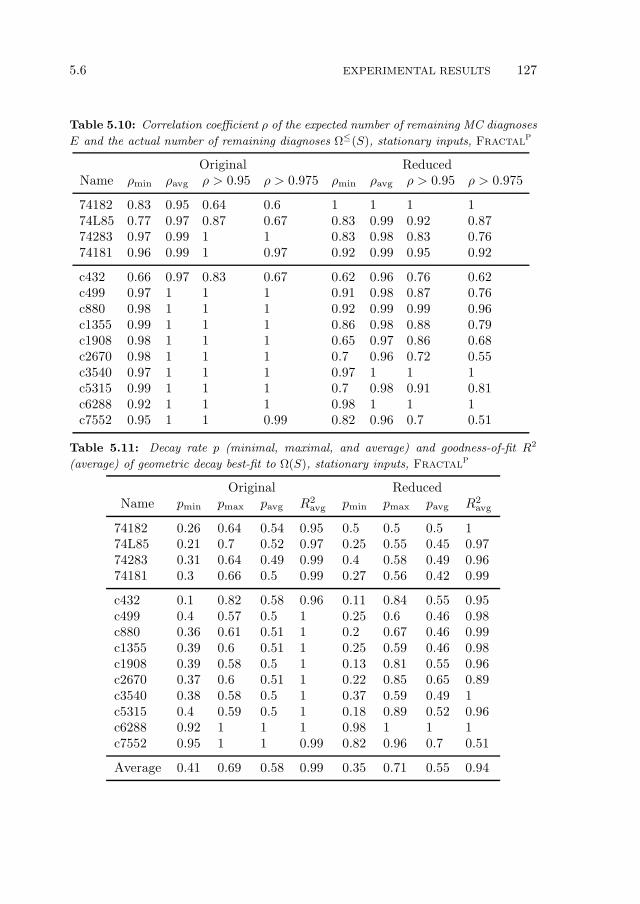
5.6 EXPERIMENTAL RESULTS 127
Table 5.10: Correlation coefficient ρ of the expected number of remaining MC diagnoses
E and the actual number of remaining diagnoses Ω≤(S), stationary inputs, FractalP
Original ReducedName ρmin ρavg ρ > 0.95 ρ > 0.975 ρmin ρavg ρ > 0.95 ρ > 0.975
74182 0.83 0.95 0.64 0.6 1 1 1 174L85 0.77 0.97 0.87 0.67 0.83 0.99 0.92 0.8774283 0.97 0.99 1 1 0.83 0.98 0.83 0.7674181 0.96 0.99 1 0.97 0.92 0.99 0.95 0.92
c432 0.66 0.97 0.83 0.67 0.62 0.96 0.76 0.62c499 0.97 1 1 1 0.91 0.98 0.87 0.76c880 0.98 1 1 1 0.92 0.99 0.99 0.96c1355 0.99 1 1 1 0.86 0.98 0.88 0.79c1908 0.98 1 1 1 0.65 0.97 0.86 0.68c2670 0.98 1 1 1 0.7 0.96 0.72 0.55c3540 0.97 1 1 1 0.97 1 1 1c5315 0.99 1 1 1 0.7 0.98 0.91 0.81c6288 0.92 1 1 1 0.98 1 1 1c7552 0.95 1 1 0.99 0.82 0.96 0.7 0.51
Table 5.11: Decay rate p (minimal, maximal, and average) and goodness-of-fit R2
(average) of geometric decay best-fit to Ω(S), stationary inputs, FractalP
Original ReducedName pmin pmax pavg R2
avg pmin pmax pavg R2avg
74182 0.26 0.64 0.54 0.95 0.5 0.5 0.5 174L85 0.21 0.7 0.52 0.97 0.25 0.55 0.45 0.9774283 0.31 0.64 0.49 0.99 0.4 0.58 0.49 0.9674181 0.3 0.66 0.5 0.99 0.27 0.56 0.42 0.99
c432 0.1 0.82 0.58 0.96 0.11 0.84 0.55 0.95c499 0.4 0.57 0.5 1 0.25 0.6 0.46 0.98c880 0.36 0.61 0.51 1 0.2 0.67 0.46 0.99c1355 0.39 0.6 0.51 1 0.25 0.59 0.46 0.98c1908 0.39 0.58 0.5 1 0.13 0.81 0.55 0.96c2670 0.37 0.6 0.51 1 0.22 0.85 0.65 0.89c3540 0.38 0.58 0.5 1 0.37 0.59 0.49 1c5315 0.4 0.59 0.5 1 0.18 0.89 0.52 0.96c6288 0.92 1 1 1 0.98 1 1 1c7552 0.95 1 1 0.99 0.82 0.96 0.7 0.51
Average 0.41 0.69 0.58 0.99 0.35 0.71 0.55 0.94
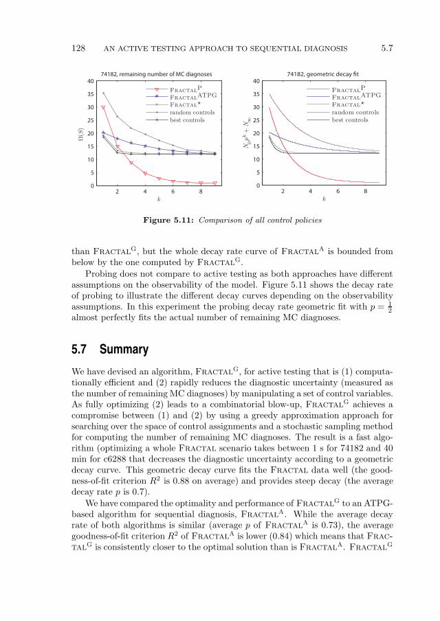
128 AN ACTIVE TESTING APPROACH TO SEQUENTIAL DIAGNOSIS 5.7
2 4 6 80
5
10
15
20
25
30
35
40
k
74182, remaining number of MC diagnoses
FractalP
FractalATPG
Fractal⋆
random controlsbest controls
2 4 6 80
5
10
15
20
25
30
35
40
k
N0p
k+
N∞
74182, geometric decay !t
FractalP
FractalATPG
Fractal⋆
random controlsbest controls
Ω(S
)
Figure 5.11: Comparison of all control policies
than FractalG, but the whole decay rate curve of FractalA is bounded frombelow by the one computed by FractalG.
Probing does not compare to active testing as both approaches have differentassumptions on the observability of the model. Figure 5.11 shows the decay rateof probing to illustrate the different decay curves depending on the observabilityassumptions. In this experiment the probing decay rate geometric fit with p = 1
2almost perfectly fits the actual number of remaining MC diagnoses.
5.7 Summary
We have devised an algorithm, FractalG, for active testing that is (1) computa-tionally efficient and (2) rapidly reduces the diagnostic uncertainty (measured asthe number of remaining MC diagnoses) by manipulating a set of control variables.As fully optimizing (2) leads to a combinatorial blow-up, FractalG achieves acompromise between (1) and (2) by using a greedy approximation approach forsearching over the space of control assignments and a stochastic sampling methodfor computing the number of remaining MC diagnoses. The result is a fast algo-rithm (optimizing a whole Fractal scenario takes between 1 s for 74182 and 40min for c6288 that decreases the diagnostic uncertainty according to a geometricdecay curve. This geometric decay curve fits the Fractal data well (the good-ness-of-fit criterion R2 is 0.88 on average) and provides steep decay (the averagedecay rate p is 0.7).
We have compared the optimality and performance of FractalG to an ATPG-based algorithm for sequential diagnosis, FractalA. While the average decayrate of both algorithms is similar (average p of FractalA is 0.73), the averagegoodness-of-fit criterion R2 of FractalA is lower (0.84) which means that Frac-
talG is consistently closer to the optimal solution than is FractalA. FractalG

5.7 SUMMARY 129
has achieved better exponential decay compared to all algorithms except exhaus-tive control search. For example, the difference in the decay rate p betweenFractalG and exhaustive search for 74182 is 5.4%. The exhaustive control ap-proach, however, takes minutes to complete even for a circuit as simple as 74182,and times-out with any model having more than 20 controls. As a result, wecan conclude that FractalG trades off a small decrease in p for a significantperformance speedup.

130 AN ACTIVE TESTING APPROACH TO SEQUENTIAL DIAGNOSIS 5.7
Chapter 6Conclusions
In this dissertation we presented a new family of MBD reasoning algorithms thatsignificantly improve the computational performance of state-of-the-art existingones while minimizing the loss of optimality. To achieve this we have used approx-imation methods, and a number of techniques such as “inverted” search, greedymethods, and stochastic sampling.
6.1 Contributions
In summary, our major contributions can be stated as follows:
Framework and Formalism: This thesis represents multiple MBD problemssuch as minimal-diagnosis, MFMC, and test sequencing in a common con-sistency-based theoretical framework. This facilitates comparison and eval-uation of results, and analysis and reuse of techniques.
Algorithms and Empirical Evaluation: The three major algorithms of thisthesis (Safari, Miranda, and FractalG) efficiently solve worst-case NP-hard or worse problems by trading small degradation in the optimality ofthe diagnostic results for much larger gain in the computational perfor-mance (in some cases several orders-of-magnitude improvement in speed).This efficient trade-off is partly due to exploitation of specific propertiesin the search landscape of the diagnostic problems. All three algorithmsachieve good optimality at low computational cost in diagnostic search prob-lems that exhibit certain amount of continuity. Empirical evaluation on theISCAS85/74XXX benchmark of combinational circuits quantitatively sup-ports our claim that benchmark diagnostic problems are amenable to thegreedy stochastic approaches described in this thesis.
131
132 CONCLUSIONS 6.1
The major highlights and contributions of the algorithms introduced in this thesisare outlined as follows:
Safari: With this algorithm we propose a novel approximation approach for com-puting multiple-fault diagnoses. Safari sacrifices guarantees of optimality,but for diagnostic systems in which faults are described in terms of an ar-bitrary deviation from nominal behavior Safari can compute diagnosesseveral orders of magnitude faster than competing algorithms.
We have demonstrated the performance gains of Safari on models having19 up to 3 512 components, involving up to 7 232 variables. The maximumtime for computing a single minimal diagnosis varies between 1 ms and 7 s.For comparison, CDA∗ times out on most experiments involving circuitswith more than 383 components and HA∗ times out on most models withmore than 546 components. Further, the computational performance of allthe algorithms we have compared to, rapidly deteriorates when increasingthe cardinality of the minimal-cardinality diagnosis, whereas the perfor-mance of Safari does not change significantly. Even SLS-based Max-SATdiagnostic methods are at least an order of magnitude slower than Safari
(or less optimal).
The decrease of optimality in Safari due to the approximation approachis small. With single-faults and weak-fault models of the 74XXX/ISCAS85circuits, the average cardinality of the diagnoses computed by Safari is 1.13(13% worse than the optimum), and with double-faults, it is 2.22 (11% worsethan the optimum). Furthermore we have shown (analytically and empiri-cally) that the performance of Safari does not depend on the cardinalityof the cardinality-minimal diagnosis.
To achieve optimality, Safari relies on a degree of continuity in the diag-nostic model. Theory shows that a large class of models (weak-fault mod-els) are continuous. Experiments with “stuck-at” 74XXX/ISCAS85 modelsshow that observations either lead to zero diagnoses (inconsistent model andobservation) or they lead to large number of diagnoses due to continuousdiagnostic subspaces. This implies the existence of a phase transition regionin the computation of minimal diagnosis, similar to the one in SAT [Gentand Walsh, 1994] where all diagnostic instances derived from combinationalcircuits are in the “easy” region.
Safari has been validated on a wide range of combinational circuits (weak-and strong-fault models of different size) but not on temporal or multi-valued encodings [Feldman et al., 2006]. Models with state are known to beless constrained than combinational ones [Hamscher and Davis, 1984], hencewe expect Safari to achieve a similar optimality vs. performance trade-off.
We have applied Safari to two real-world problems: ADAPT (cf. Ap-pendix B and PIM (cf. Appendix C) where we have modeled the physical
6.1 CONTRIBUTIONS 133
systems using the Lydia modeling language (cf. Appendix A). The sys-tems are beyond trivial, having tens of components. The results show thatthe Safari approach provides good precision metrics for only a fractionof the computational time of competing algorithms. In addition to theapplications outlined in this thesis, the Lydia/Safari approach has beensuccessfully applied to production-level troubleshooting of semiconductormanufacturing equipment [Pietersma and van Gemund, 2007].
Miranda: Miranda computes observation vectors leading to faults of high car-dinality as an approximation to MFMC observation vectors. The MFMCvalues computed by Miranda are optimal for 74XXX and 88% of the min-imum for c432 (c432 has been brute-forced by de Kleer [2008]). For smallcombinational circuits (74XXX) Miranda computes MFMC observationsseveral orders of magnitude faster than exhaustive algorithms. With largecircuits, Miranda was able to compute an MFMC observation vector lead-ing to a diagnosis of approximate cardinality of 36 in less than 6 min (c5315).The reason for the good Miranda performance is the fact that it exploitscontinuity in the space of output assignments in a class of well-formed bench-mark circuits.
The implementation of Miranda in this thesis uses as a diagnostic ora-cle Safari, configured to compute subset-minimal diagnoses. This, and thegreedy nature of Miranda result in observation vectors that are“best effort”approximations of MFMC diagnoses. Hence, Miranda overestimates theMFMC numbers due to the use of Safari and underestimates the MFMCnumbers due to its greedy nature. The combination of the above errorfactors results in a smaller overall error. Due to the fact that computingMFMC vectors is ΣP
2 -complete (cf. Sec. 4.3) and the fact that Miranda ac-cepts fault-models of circuits implementing arbitrary Boolean functions, wehypothesize that there is no algorithm below ΣP
2 that can compute boundedapproximations of MFMC observation vectors.
In this thesis and in related publications [Kurtoglu et al., 2009], we haveseen empirical evidence that the performance of existing MBD algorithmsquickly deteriorates when increasing the cardinality of the injected faults(an MBD algorithm based on W-MaxSatz, for example, was unable tocompute c499 diagnoses of cardinality higher than 1 in 5 min). As theobservations leading to high-cardinality faults were computed by Miranda,we can conclude that our implementation of Miranda delivers observationvectors of high optimality at acceptable computational cost.
Fractal: We have devised an algorithm, FractalG, for sequential diagnosis,that computes near-optimal control assignments for reducing the diagnosticuncertainty (the number of remaining MC diagnoses). As fully optimizingthe decay of the number of remaining MC diagnoses leads to a combinato-rial blow-up, FractalG offers an optimality vs. speed trade-off by using

134 CONCLUSIONS 6.2
a greedy approximation approach for searching in the space of control as-signments, and a stochastic sampling method for estimating the number ofremaining MC diagnoses. The result is a fast algorithm (computing a wholeFractal scenario takes between 1 s for 74182 and 15 min for c7552) thatdecreases the diagnostic uncertainty according to a near-geometric decaycurve. The reason for the efficiency of FractalG is that it exploits conti-nuity in the space of control assignments. Experimentation shows that thisis true even for a small number of control inputs.
FractalG has achieved better exponential decay compared to alternativeapproaches, except exhaustive control search. The difference in the decayrate p between FractalG and exhaustive search for 74182 is 5.4%. Theexhaustive control approach, however, takes minutes to complete even for74182 and times out with any model having more than 20 controls. As aresult we can conclude that FractalG trades a small decrease in p for asignificant performance speedup.
There are two challenges in applying MBD to real-world problems: (1) the model-ing challenge [Narasimhan, 2002] and (2) the computational complexity of MBD.The two challenges are related. Models of complex physical systems have thou-sands to millions of variables [Provan and Wang, 2007] and abstracting at suchmagnitude is a significant challenge to modelers. The burden of manually ab-stracting (reducing the model complexity) can be alleviated by creating algo-rithms that can efficiently solve large systems. This would also facilitate, to someextent, automated translation from design specifications. This thesis helps solv-ing the computational problem thus bringing MBD one step closer to large-scale,practical diagnosis of complex physical systems.
6.2 Improvements and Future Work
This thesis involves computer scientific, mathematical, and statistical disciplinessuch as complexity theory, satisfiability, ATPG, automated reasoning, optimiza-tion, experimental design, and others. As the main purpose of this dissertationis to substantiate the claims made in the introduction, not all aspects have beentreated exhaustively.
What follows is a list of proposals for improving each of the algorithms pre-sented in this thesis, followed by other suggestions for future work.
Algorithms Presented in this Thesis
Safari: The search performance of Safari can be improved for multiple diag-noses by adding “beam-search” capabilities to the algorithm. This meansthat once a subset-minimal diagnosis is found, the search does not restart,but continues with perturbing the diagnosis, thus searching for new diag-noses in the neighborhood of the existing one. This will lead to nearly
6.2 IMPROVEMENTS AND FUTURE WORK 135
quadratic improvement in the time-complexity of Safari. Our estimate isbased on (1) the average complexity of Safari and (2) the practical observa-tion that faults usually propagate in their immediate neighborhood. Inter-estingly, (2) is also supported by analyzing combinational circuits. ISCAS85observations, for example, lead more often to cliques of faulty components(these are subsets of components that can fail in any combination) than tofaults dispersed throughout the whole circuit. The latter is due to circuitdesign and is related to model continuity as discussed in this thesis.
An approach to increase the utility metric of Safari diagnoses is to usea more precise ordering of the diagnostic results based on different priorprobabilities and conflicts. It is straightforward to convert Safari to workon the dual problem of computing minimal diagnoses: computing minimalconflicts. One can show that in this case most properties and bounds ofSafari still apply. After computing diagnoses from conflicts, one can usea Bayesian technique such as Barinel [Abreu et al., 2009] for computinga posteriori fault probabilities. Considering only the first k diagnoses withhighest a posteriori probability will improve precision-based metrics such asnumber of classification errors and utility.
Miranda: The Miranda algorithm offers ample opportunities for further devel-opment. Unlike the other two algorithms, the absolute CPU performanceof Miranda is of secondary importance and the main goal is to improvethe cardinality of the Miranda observations. One way to improve Mi-
randa optimality is to use model decomposition. We have seen in Chap-ter 4 that MFMC is related to model decomposition (i.e., the number ofvariables shared by subsystems) and we hypothesize that the error in theMFMC approximations of Miranda can be bounded by model decomposi-tion parameters (e.g., the maximum number of variables shared by differentsubsystems). The optimality of the MFMC approximations can be furtherimproved by studying, quantifying, and using the notion of circuit “well-formedness”. For example, the number of reconverging outputs in a circuitcan be used for adjusting the MFMC search policy.
Fractal: The computational efficiency of the Fractal algorithm can be im-proved at least an order-of-magnitude by eliminating unnecessary computa-tion. In particular, during search, FractalG, can compute and cache singleinput values ruling out certain diagnoses. The consistency of assignmentscontaining these cached values can be determined quickly (in logarithmictime) by performing cache look-ups. This approach is similar to conflictlearning in satisfiability or structure exploitation in diagnosis [Feldman andvan Gemund, 2006].
The performance of FractalG can be improved by using topological prop-erties of the model. For example, if two controls are independent, they canbe applied simultaneously for a faster decay of the number of diagnoses.
136 CONCLUSIONS 6.2
The decay speed of FractalG can be also improved by “learning”probabil-ities of observations from multiple applications of the algorithm on a givensystem.
Other Suggestions for Future Work
The algorithms presented in this thesis can be generalized and combined withapproaches from other AI and computer science disciplines. In what follows weoutline several potential high-impact applications of the approximation algorithmswe have proposed.
Diagnosis of Systems with State: This thesis largely abstracts from the tem-poral behavior of systems. Although some elementary time-related proper-ties can be modeled in Lydia (for example by adding an extra array dimen-sion to each variable), Lydia has no built-in mechanisms for representingtime and temporal constraints. As a step toward fusion of combinationalMBD and Discrete Event Systems (DES) algorithms [Sampath et al., 1994],one can introduce time delays and/or flip-flops in Lydia. Flip-flops in Ly-
dia would allow experiments with Safari on models of the ISCAS89 [Brglezet al., 1989] sequential circuits.
Provan [2009] has introduced a mechanism for translating hybrid automatato Lydia propositional models that has been applied to a small industrialcase [Behrens et al., 2009]. The results so far do not extend to larger mod-els. Applying Safari to discrete models of complex hybrid systems willresult to at least an order-of-magnitude speedup compared to deterministicalgorithms.
Max-Fault ATPG: Automated testing of Very Large-Scale Integration (VLSI)circuits [Bushnell and Agrawal, 2000] is a multi-million dollar industry. Mi-
randa offers near-theoretical compaction of ATPG sequences which is asignificant progress compared to the single-fault “don’t care” compactionmethods used today. We hypothesize that, depending on the IC topology,stochastic MFMC-based ATPG algorithms offer near-optimal coverage andat least 70% reduction in the size of the testing sequences. This is a con-servative estimate based on study of existing ATPG compaction techniques.Corno et al. [1997] show a method that performs static compaction of ATPGsequences and achieves 50% to 62% improvement in the size of the test set.The latest dynamic compaction methods report a 23% improvement com-pared to static methods [Czutro et al., 2009] and an MFMC-based ATPGwould approach the theoretical limit which, so far, has not been established.
Discretization and Learning of Sensor Data: As is visible from the diag-nostic competition, Appendix B, and other real-world examples, many sen-sor readings such as temperature, voltage, current, or pressure, are suppliedas continuous values in the real domain. The MBD approaches described in

IMPROVEMENTS AND FUTURE WORK 137
this thesis (and most of the referred algorithms) work with discrete variables.Hence, a real-world application has to discretize continuous sensor readingsoutside the MBD framework. In our application experiments with Lydia wedo this in an ad-hoc manner and existing literature and applications largelyneglect this aspect of diagnosis.
The commercial package for MBD RODON [Lunde et al., 2006] uses interval-based logic but leaves the problem of computing the interval boundaries tothe user. Even hybrid algorithms like HyDE [Narasimhan and Brownston,2007] that allow real valued variables need to manually include conditionsand landmark values for modeling system transitions. A potential futureresearch with high impact on applying MBD techniques to real-world appli-cations would be to use learning and signal processing methods to discretizesensor values. Automatic identification of nominal sensor readings is atleast as complex as computation of diagnosis but if implemented, it wouldsimplify the modeling process.
Automated Design for Reliability: Approximation MBD techniques can beused for tasks beyond diagnosis such as model-based design and redesign.We have already demonstrated that a technique based on MBD provides bet-ter trade-offs in adding system redundancy for increasing system reliabilitycompared to traditional approaches [Feldman et al., 2009a]. Model-baseddesign and redesign problems typically expose higher complexity than MBDproblems. For example, one can formulate problems of generating or modify-ing system descriptions that are undecidable, and approximation algorithmshave no alternative in approaching the intractability of these problems. Wehave already seen successful application of AI approaches like satisfiabilityto Computer-Aided Design (CAD) [Gu and Puri, 1995]. Although diagnos-tic and abductive reasoning is more complex than satisfiability, advances inalgorithmic performance like the one presented in this thesis would allowthe application of MBD to large-scale design and redesign problems leadingto reduction in design labor and more optimal troubleshooting of designspecifications.
As some of the above examples show, we expect approximation MBD algorithms toperform well on problems beyond diagnosis. Most of the MBD problems describedin this thesis are close to logic-based abduction [Console et al., 1991] and can besolved with methods from abductive reasoning. This implies to some extent thatthe diagnostic techniques described in this thesis can be used for addressing awider spectrum of abduction problems.

138 CONCLUSIONS
Appendix AThe LYDIA Modeling Language
We have designed a low-level language for system modeling called Lydia (Lan-guage for sYstem DIAgnosis). Lydia is also the framework in which are developedall the algorithms in this thesis. The Lydia tool-kit also contains model transla-tors (e.g., to CNF, DNF, OBDDs, etc), utilities, and reference implementation ofalgorithms such as CDA∗, HA∗, and others. The initial design and implementa-tion of Lydia can be found in van Gemund [2002, 2003]. All the material in thisthesis corresponds to version 2.0 of Lydia. This appendix presents an up-to-dateoverview of the Lydia language syntax and semantics.
Lydia models are collections of systems. Each system represents a componentor a subsystem. Lydia systems are introduced in Sec. A.1 where we also showthe model of a small combinational circuit (a full-adder). In this early examplewe use variables and constraints intuitively. Section A.2 explains the basic Lydia
expressions. Lydia variables and data types are discussed in detail in Sec. A.3.Lydia expressions are discussed in Sec. A.4. Finally, Sec. A.5 discusses Lydia
predicates.
A.1 Systems and Subsystems
Synthetic and real-world systems have hierarchical structure which is representedin a Lydia model by using systems, subsystems and system instantiations. Thestructure of a Lydia model can be represented as multidigraph in which each sys-tem is a nodes and each instantiation is an edge. Lydia preserves this structuralinformation until, explicitly “flattened-out” in the model translation pipeline ashierarchy exploitation has the potential of speeding-up the reasoning process.
A system declaration includes the keyword system, the system name and alist of formal parameters. System declarations conform to the following syntax:
139

140 APPENDIX A
system <name> (<type1> <formal1>, [<type2>] <formal2>, . . .)
...
Any valid Lydia identifier1 can be used for the system name. A system may havezero, one or more formals. Similar to when declaring local variables, subsequentidentical formal types may be omitted.
ci
i1
i2
co
Σ
h1
h4
h3
h5
h2
Figure A.1: A full adder
We show the use of systems and subsystems and some basic Lydia constructs bymodeling the Boolean full-adder shown in Fig. A.1. A full-adder consists of fivelogic-gates: an or-gate, two and-gates, and two xor-gates. Each of these threecomponent types will be modeled as a Lydia system. Note that Lydia doesnot have an explicit notion of a component. Lydia uses assumable (or health)variables to denote components. What follows are weak-fault2 models of the threebasic gate types.
system xor2(bool o, i1, i2)
bool h;attribute probability(h) = (h ? 0.9999 : 0.0001);
attribute health(h) = true;
h => (o = (i1 != i2));
1Valid Lydia identifiers are sequences of alphanumeric characters or the underscore, startingwith a letter.
2For a discussion on fault-modeling strength, cf. Chapter 2.

SYSTEMS AND SUBSYSTEMS 141
system and2(bool o, i1, i2) 10
bool h;attribute probability(h) = (h ? 0.9999 : 0.0001);attribute health(h) = true;
h => (o = (i1 and i2));
system or2(bool o, i1, i2) 20
bool h;attribute probability(h) = (h ? 0.9999 : 0.0001);attribute health(h) = true;
h => (o = (i1 or i2));
Each of the above systems has three formal parameters3: an output o and twoinputs (i1 and i2 ). In each system there is a Boolean variable h that has the extra“health” and “probability” attributes. These two attributes make all h variablesassumables. Finally, a single Lydia predicate models the nominal behavior of thegate. We will discuss variables and constraints in the sections that follow.
A full-adder is composed of two half-adder, each of which consists of an xor-gate and an and-gate. A model of a half-adder is shown below.
system halfadder2(bool i1, i2, sum, carry)
system and2 A(carry, i1, i2);system xor2 X(sum, i1, i2);
Finally, two half-adders and an or-gate are connected (instantiated) in the finalmodel:
system fulladder2(bool i1, i2, ci, sum, carry)
bool f, p, q;
system halfadder2 HA1, HA2;
HA1(i1, i2, f, p);HA2(ci, f, sum, q);
system or2 O(carry, p, q); 10
3Referred to as ports in HDL languages such as VerilogTM.

142 APPENDIX A
A.2 Basic Expressions
A Lydia expression is a formula over the standard propositional operators ¬(negation), ∧ (conjunction), ∨ (disjunction), ⇒ (implication), and ⇔ (equiva-lence). Negation is typed as “!” or, alternatively, as the keyword “not”. Con-junction can be typed as “&&” or textually as “and” and disjunction is denotedboth by the symbolic “||” and mnemonic “or”. Implication is denoted as “=>”and equivalence either as “=” or “==”.
To illustrate the use of the above five operators we will use simulation tocompute the value of the Boolean function
f(x, y, z) ≡ x ∧ ¬y ∨ (z ⇒ y)⇔ z (A.1)
In our example we will evaluate f(1, 1, 0). The function is implemented in thefollowing four-variable model:
system expr(bool f, x, y, z)
attribute observable(x, y, z) = true;
f == (x && !y | | (z => y) = z);
The value (1, 1, 0) at which we want to see f evaluated is specified as the followingobservation:
observation alpha 1
x && y && !z;
Finally, we invoke Lydia with the simulation option. The result is shown below.
lydia> sim expr alpha_1
x = true, y = true, f = false, z = false
A.3 Data Types
A Lydia model is variable-centric, that is, it specifies the properties of a systemas a set of constraints over one or more variables. In the reasoning process, thesevariables are always treated separately (i.e., early in the translation process arraysand structures are broken down into their elements). The Lydia language allowsrich variable-type semantics, resulting in short and expressive models. In whatfollows we discuss the built-in Lydia variable data-types and the primitives fordefining user-types.

DATA TYPES 143
A.3.1 Atomic Data Types
Lydia has two atomic variable types: Booleans and enumerations. The formerexists for convenience and for more aggressive optimization in the tool-kit (if theBoolean type was not built-in, a user could have easily introduced an enumerationdefining it). A Lydia modeler needs to declare all variables before using them.A variable declaration can be done either in the list of formal parameters of asystem or in the system body.
system Bar(bool v1, v2, bool v3, . . . , vn)
...
Good modeling style avoids unnecessary variables in the formal parameter listof a system – sharing variables makes models difficult to read and hinders theperformance of some hierarchical diagnostic reasoners [Feldman and van Gemund,2006].
The order of Lydia statements is in most cases irrelevant for the model. Ly-
dia even does not make mandatory to declare a type or a variable before usingit (declarations are mandatory, no matter if a declaration is before or after a cor-responding defintion). An enumeration, for example, can be defined anywhere inthe global scope of a model. An enumeration specifies a set of symbols that areallowed for a variable of a given type. Consider an example where a variable oftype color can be either red or green or blue:
type color = enum red, green, blue ;
Once we have declared the color type, it can be used anywhere in the model asillustrated in the following model excerpt:
system ColorMixer(color in1, in2, out1, out2)
color common;...
Constant types should be always explicitly specified as in the right hand side ofthe Lydia expression shown below. Having the color type declaration from above,we can assert the value of the internal variable common in the following manner:
common = color.red;
Note, that due to the semantics of the enumerations, a variable of type color canbe either red or green or blue but it can assume exactly one value. Hence, anysystem containing an expression like:
(common = color.red) && (common = color.blue);

144 APPENDIX A
is trivially inconsistent, while the following constraint simplifies to true:
(common = color.red) | | (common = color.green) | | (common = color.blue);
A.3.2 Composite Data Types
Lydia modelers can use arrays and structures to group related variables. Inaddition to that, the Lydia language allows type aliasing.
Arrays
A Lydia model can use arrays of any type and dimension. These arrays are“broken down”into sets of variables at compile4 time, hence only statically-definedarrays are allowed. Unlike other languages, arrays may start from any index. Wewill illustrate the use of arrays by solving the well-known N-Queens problem. Themodel, shown below, defines the chess-board as a two-dimensional array of typebool. Placing a queen on the chess board will be expressed as assigning True tothe respective member of the array. Below is the full N-Queens Lydia model:
const int N = 6;
system nqueens()
bool board[1:N][1:N];
forall (i in 1 . . N) exists (j in 1 . . N) /* At Least One */
board[i][j]; 10
forall (k in 1 . . N − 1) /* At Most One */forall (l in k + 1 . . N)
!board[i][k] | | !board[i][l];!board[k][i] | | !board[l][i];
forall (i in 1 . . N − 1) /* At Most One */forall (j in 1 . . N − i) 20
forall (k in 1 . . N − i − j + 1) !board[i + j − 1][j] | | !board[i + j + k − 1][j + k];!board[j][i + j − 1] | | !board[j + k][i + j + k − 1];!board[N − i − j + 2][j] | | !board[N − i − j − k + 2][j + k];!board[N − j + 1][i + j − 1] | |
4We mean non-strict compilation, that is a translation to some normal form, e.g., a Conjunc-tive Normal Form (CNF).

DATA TYPES 145
!board[N − j − k + 1][i + j + k − 1];
30
To solve the N-Queens problem we have to impose a number of constraints. To dothis we use quantifiers (cf. Sec. A.5.3) that specify that there is at least one queenin every row (or column) and at most one queen per row, column and diagonal ofthe board. Note, that for convenience, we started our arrays from one.
6 0Z0l0Z5 l0Z0Z04 0Z0ZqZ3 ZqZ0Z02 0Z0Z0l1 Z0l0Z0
a b c d e f
6 0l0Z0Z5 Z0ZqZ04 0Z0Z0l3 l0Z0Z02 0ZqZ0Z1 Z0Z0l0
a b c d e f
Figure A.2: Two of the four solutions of the 6-queens problem
An array declaration, like a variable declaration, can appear anywhere in a systemand should adhere to the following syntax:
<type> <name> [s1 : e1][s2 : e2] . . . [sn : en];
In the syntax definition above, <type> is any atomic or composite type, <name>is a valid Lydia identifier and si, ei (i = 1, 2, . . . , n) are integers specifying thefirst and last elements of the array5. Alternatively, one can define arrays in aC-like manner, specifying only the size of each dimension.
<type> <name> [d1][d2] . . . [dn];
In the excerpt below, the declarations of the cubeX and cubeY arrays are ofequivalent type.
bool cubeX[0:7][0:7][0:7];bool cubeY[8][8][8];
5It is not necessary that si < ei.

146 APPENDIX A
Structures
Variables can be grouped in structures. The latter are simply naming conve-niences, as variables in structures share common suffixes (the names of the struc-tures). The structures are expanded by Lydia into separate variables at compiletime. Consider several of the type definitions from the X-34 domain shown next.
type range = enum below, inside, above ;type fluid = enum helium, LO2, RP1 ;
type line = struct
range pressure,range temperature,fluid contents
;
The third type definition combines the pressure, temperature and contents vari-ables in a structure defining a pipe. Lydia imposes no restrictions on the types ofthe structure members. In the example above, the three member variables are allof enumeration types, while a structure member can be also a (nested) structure,or even an array (cf. Sec. A.3.2). This allows for a fairly complex compositeLydia data types.
Continuing our line structure example, we declare line instances and use theseinstances for defining system constraints. This is illustrated in the following modelfragment:
system PneumaticValveAndMicroSwitch(line i, o, c)
valveState state;microSwitchState microSwitch;
...
if ((state = valveState.open) or (state = valveState.stuckOpen)) o = i;
10
if ((state = valveState.closed) or (state = valveState.stuckClosed)) o.pressure = range.below;
The above excerpt (from a model of a pneumatic valve) defines three formalvariables of the structure type line. These are named i, o and c. The consequentof the first if construct states that all member variables of i should be equalto all member variables of o. Hence, o = i is a shortcut for the following set of

DATA TYPES 147
constraints:
i.pressure = o.pressure;i.temperature = o.temperature;i.contents = o.contents;
Type Aliases
Type aliasing is part of the Lydia typing system. Here is an example of how wecan define a type bar, introduce a type foo that is an alias of bar and use the newfoo type for instantiating a variable:
type bar = enum red, green, blue ;type foo = bar;
system main()
foo color = bar.green;
A.3.3 Variable Attributes
A Lydia variable may carry attributes. Attributes have no universal semanticsin the Lydia language. Attributes can be used to carry application specific infor-mation for the end user, or, for applications using Lydia.
An attribute assigns data to each value a variable may assume. This is bestillustrated with an example. Suppose we have a variable k of type color (cf. thetype definition of color in Sec. A.3.1). The variable k, can assume the valuesred, green, or blue. We can declare an attribute rgb of type int and assign anumeric value for each of the k values (red, green, or blue). After the diagnosis(or simulation) process computes values for k, the respective numerical attributescan be retrieved by the application that uses Lydia.
There are three special built-in variable attribute types in Lydia that do nothave to be declared: probability, health, and observable. We have already seenthese three attributes in the preceding examples and will discuss them in moredetail below. These three attributes are used by all diagnostic solvers.
Lydia attribute are typed. Attributes can be of type bool, int, float, andstring. The variable attributing mechanism is limited in expressiveness, and doesnot allow user-defined types. A variable attribute declaration has the followingsyntax:
attribute <type> <name>
A Lydia attribute assigns a value for each possible value a variable may assume.Any expression for which all values of a variable can be precomputed at modelcompilation time can be used as a variable attribute. Note that all except thethree built-in attribute types should be declared at the global scope. Variable

148 APPENDIX A
attributes are defined in the same scope where the variables are defined (theorder is irrelevant). Both formal and local variables can have attributes. Whatfollows is the syntax of a variable attribute declaration.
attribute <name> (<variable1>, <variable2>, . . . , <variablen>) = <expression>
The simplest variable attributes assign constant values to variables.We next discuss the three built-in attribute types. We have already mentioned
that the observable attribute has a special meaning in Lydia. Variables, whichhave this attribute specified, may get their values from the user, i.e., they can beobserved.
Consider a model of an inverter. It has its input and output variables i and omarked as observables and starts as follows:
system inverter(bool i, o)
attribute observable(i, o) = true;...
We use h for the health of the above inverter. To mark a variable as healthor assumable (the latter two are synonyms) we have to assign a pair of built-in attributes: probability and health. The former is of type float, while thelatter is of type bool. We continue the inverter model with assigning those twoattributes to h:
...attribute probability(h) = (h ? 0.95 : 0.05);attribute health(h) = h;
The first attribute specifies that h is 0.95 for h = true, and 0.05 for h = false.Note that all a priori probabilities must sum to unity (otherwise the Lydia modelcompiler will produce a warning message). The health attribute specifies whena component is “healthy”. In the model continuation below the inverter will behealthy when h = true, otherwise, for h = false, it is broken (or faulty).
As an alternative to the above two attributes we can use f = false to denotea faulty gate (thus inverting the health logic) in the following way:
...attribute probability(f) = (f ? 0.01 : 0.99);attribute health(f) = !f;
The two lines above specify that the prior fault probability of f = false is 0.99and that of f = true is 0.01. The meaning of the health attribute is inverted incomparison to h, i.e., f is faulty for f = false.

DATA TYPES 149
Having discussed the three built-in attributes, we continue our discussion withan example on the use of user-defined attributes. The model excerpt below de-clares three user type attributes. These can be used in a model, where, for exam-ple, we would like to attach user-supplied data to some health variables. After thecomputation of diagnosis, this data can be used for locating the faulty componentor computing cost of repair, etc.
...attribute string location;attribute float cost;attribute bool input;
...
The part from the Lydia system description, shown next, uses the three newlydefined attribute types (location, cost, and input) to attach user-supplied valuesto the variable h.
...attribute cost(h) = h ? 97.5 : 2.5;attribute input(h) = true;attribute location(h) = "quadrant 12";
...
In the above case the input and location attributes are constant for every valueof h.
As we have seen from the observable attribute, it is possible to attributemultiple variables with a single statement. In our example, however, the attributehad a constant value. The probability, for example, is different depending on thevalue of h, hence the expression h ? 0.95 : 0.05. The above example would notwork if we try to attribute multiple variables at the same time due to the fact thath is mentioned in the right-hand side of the attribute expression. For example,trying to compile:
system main()
bool h1, h2;
attribute probability(h1, h2) = h1 ? 0.95 : 0.05;
would lead to the following error:
err.sys:5: error: can’t evaluate probability(h2) for h2 = false
err.sys:5: error: (Each non-evaluated value is reported only once
err.sys:5: error: for each attribute it appears in.)

150 APPENDIX A
As the alternative of attributing each variable separately is cumbersome, Lydia
allows the use of attribute aliases in the attribute expression as illustrated next:
attribute probability(h1, h2) = \x x ? 0.95 : 0.05;
In this case x will alias first h1 and then h2 and both h1 and h2 will receive thesame a priori probability. Only variable of the same type can be attributed inthis way. The same technique may be used for attributing variable arrays, as isshown in the example below:
bool g[4][4];
attribute probability(g) = \x x ? 0.99 : 0.01;attribute health(g) = true;
When attributing arrays, it is also possible to attribute all the elements of thearrays separately, or in groups:
bool z[3];
attribute observable z[0:1] = true;attribute health z[2] = true;
Variables grouped in structures (cf. Sec. A.3.2) can be attributed by using at-tribute aliases if all variables are of the same type. The same applies for complexdata types consisting of structures and arrays. What follows is an example ofattributing all the variables in a structure:
type flow = struct bool fsign, bool fder ;
attribute float d;
system main()
flow f;
attribute d(f) = \x x ? 10 : 100; 10
The above mechanism would not work if the variables in a structure are of different
EXPRESSIONS 151
types. In this case we can use typed aliases as illustrated next:
type content = enum t1, t2, t3 ;type flow = struct bool fsign, bool fder, content c1, content c2 ;
attribute float d;
system main()
flow f;
attribute d(f) = \x::bool x ? 10 : 100; 10
attribute d(f) = \x::content cond(x) (content.t1 −> 1; content.t2 −> 2)
As we have seen, variable attributes provide a powerful macro-mechanism forattaching user-defined data to variables. In the examples we have used someLydia expressions to compute values for each value a variable may assume. Note,that the aliasing mechanism which we have seen and the int, float, and string
attribute types present in the attribute processing mechanism only and they cannot be used outside of attribute expressions.
A.4 Expressions
Lydia expressions are used for specifying variable constraints.
A.4.1 Conditional Expressions
The syntax of the arithmetic if in Lydia is similar to the one in C:
<expression1> ? <expression2> : <expression3>
Arithmetic if expressions can be nested. Each arithmetic if is internally translatedto (expression1 ⇒ expression2)∧ (¬expression1 ⇒ constraints3). The conditionalif in the inverter model below stipulates that inverter should be healthy if thevalue of its input i is equivalent to the value of its output o.
system inverter(bool h, i, o)
attribute observable(i, o) = true;attribute health(h) = h;attribute probability(h) = (h ? 0.95 : 0.05);
h ? (i == o) : (i != o);
An expression without equivalent in other languages is the conditional switch. Aconditional switch expression has the following syntax:

152 APPENDIX A
cond (<expression1>) (<expression2> –> <expression3>
...<expression2n> –> <expression2n+1>default –> <expression2n+2>
)
Denote the propositional (possibly multi-valued [Feldman et al., 2006]) Wff equiv-alent to <expressioni> as ei (1 ≤ i ≤ 2n+ 2). The Lydia compiler rewrites eacharithmetic switch expression to the following system of equations:
∣∣∣∣∣∣∣∣∣∣∣∣∣
(e1 ⇔ e2)⇒ e3(e1 ⇔ e4) ∧ ¬(e1 ⇔ e2)⇒ e5(e1 ⇔ e6) ∧ ¬(e1 ⇔ e4) ∧ ¬(e1 ⇔ e2)⇒ e7
...(e1 ⇔ e2n) ∧ ¬(e1 ⇔ e2) ∧ ¬(e1 ⇔ e4) ∧ · · · ∧ ¬(e1 ⇔ en−1)⇒ e2n+1
¬(e1 ⇔ e2n) ∧ ¬(e1 ⇔ e2) ∧ ¬(e1 ⇔ e3) ∧ · · · ∧ ¬(e1 ⇔ en−1)⇒ c2n+2
(A.2)
The use of the arithmetic switch is exemplified by the following model excerpt(part of a model of an airplane fuel switch valve):
system selectorValve(selectorPosition selector, bool enginePumpOn, · · · )
...if (h == hSelector.nominal)
flowOut == cond (selector) (selectorPosition.off −> mass.zero;selectorPosition.left −> flowLeft;selectorPosition.right −> flowRight;default −> mass.zero);
10
The above arithmetic switch specifies that if the switch selector is in “off” posi-tion, then the value of the flowOut variable should be equivalent to the constantmass.zero. Similarly, if the switch is in position “left” the value of the flowOutvariable should be equivalent to the value of the variable flowLeft, etc. Note thatthe default case can be omitted if there are corresponding expressions for all thevalues expression1 can assume. If this is not the case and a default expression isnot specified, Lydia will produce an error.

EXPRESSIONS 153
A.4.2 Qualitative Inequalities
Lydia enumeration variables can be compared. Consider the following model:
type letter = enum a, b, c, d ;
system qi()
letter x, y;
bool h;
attribute observable(x, y) = true;attribute health(h) = h; 10
attribute probability(h) = (h ? 0.95 : 0.05);
if (h) x < y;
and the two observation vectors alpha 2 and alpha 3:
observation alpha 2
(x == letter.a) && (y == letter.c);
observation alpha 3
(x == letter.c) && (y == letter.a);
Observation alpha 2 results in the empty set of diagnoses while swapping x and
y in alpha 3 results in a negative value for h as demonstrated by the transcriptbelow:
lydia> diag qi alpha_1
lydia> fm
d1 =
lydia> diag qi alpha_2
lydia> fm
d1 = h = false
Qualitative inequalities should be used with care as they may lead to combinatorialblow-ups. Consider an enumeration that can assume n values:
type <name> = enum t1, t2, . . ., tn ;

154 APPENDIX A
A qualitative inequality such as x ≤ y would be internally expanded to
[(x⇔ t1) ∧ (y ⇔ t1)] ∨(x⇔ t2) ∧ [(y ⇔ t1) ∨ (y ⇔ t2)] ∨
...(x⇔ tn) ∧ [(y ⇔ t1) ∨ (y ⇔ t2) ∨ · · · ∨ (y ⇔ tn)]
(A.3)
which is difficult for translation to a normal form (CNF or DNF).
A.5 Predicates
Lydia constraints are specified in the system bodies as sequences of predicatesseparated by semicolons. After converting all predicates to a normal form, Lydia
uses the normal forms conjunction as a system model.
A.5.1 Basic Predicates
Basic predicates contain expressions. Consider a model of a buffer:
system buffer(bool o, i)
bool h;
attribute probability(h) = (h ? 0.99 : 0.01);attribute health(h) = h;
h => (o = i);
The last line of the above model (h => (o = i)) is a basic predicate.
A.5.2 Conditional Predicates
The if predicate is one of the most-commonly used constructs in Lydia. The if
syntax is shown below.
if (<expression1>) <constraints1>
else if (<expression2>) <constraints2>
... else if (<expressionn−1>)
<constraintsn−1> else
<constraintsn>

PREDICATES 155
The if construct is a verbose way to write conditional expressions (cf. Sec. A.4.1).In the next excerpt, which comes from the plane domain, we show some typicaluse of the if predicate. The model below shows a way to build qualitative modelsof sensors, where one or more measurements should coincide with the sensorreadings (iff the sensor is functioning normally). Furthermore, the reasoner candiscern different sensor faults (the model below is of a fuel sensor), given the signof the time-derivative of a reading.
system sensor(mass real, deltaReal, indicated, deltaIndicated)
...if (h = sensorState.nominal)
indicated == real;deltaIndicated == deltaReal;
if (h = sensorState.stuckLow) (indicated = mass.zero) | | (indicated = mass.low);deltaIndicated = mass.zero;
10
if (h = sensorState.stuckHigh) indicated = mass.high;deltaIndicated = mass.zero;
It is often more elegant to model a succession of if and else if predicates as asingle switch construct. The reader ought not to be confused by the resemblanceof the Lydia switch construct to the one in some procedural languages (e.g., Cand Java). In Lydia the switch construct is used in a more powerful, higher-level, way than a sequence of if and else if predicates. The syntax of the switch
construct is the following:
switch (<expression1>) <expression2> –>
<constraints1>
...<expressionn> –>
<constraintsn−1> default –>
<constraintsn>

156 APPENDIX A
If we denote the propositional (possibly multi-valued [Feldman et al., 2006])Wff equivalent to <expressioni> as ei and the conjunction of Wff contained in<constraintsj> as cj , then the Lydia compiler rewrites every switch constructin a model to the following system of equations:
∣∣∣∣∣∣∣∣∣∣∣∣∣
(e1 ⇔ e2)⇒ c1(e1 ⇔ e3) ∧ ¬(e1 ⇔ e2)⇒ c2(e1 ⇔ e4) ∧ ¬(e1 ⇔ e2) ∧ ¬(e1 ⇔ e3)⇒ c3
...(e1 ⇔ en) ∧ ¬(e1 ⇔ e2) ∧ ¬(e1 ⇔ e3) ∧ . . . ∧ ¬(e1 ⇔ en−1)⇒ cn−1
¬(e1 ⇔ en) ∧ ¬(e1 ⇔ e2) ∧ ¬(e1 ⇔ e3) ∧ . . . ∧ ¬(e1 ⇔ en−1)⇒ cn
(A.4)
The practical use of the Lydia switch construct is illustrated in a componentmodel excerpt from the International Berthing and Docking Mechanism (IBDM)hard-docking system.
if (((motorSelector = EMAMotorSelection.primary) ?stateMotor1 :stateMotor2) = EMAState.healthy)
switch (regime) EMARegime.latching −>
(current = range.inside) => (gearOut = ringGear.latching);(current = range.above) => (gearOut = ringGear.forceLatching);
EMARegime.latched −> 10
(current = range.below) => (gearOut = ringGear.latched);
EMARegime.unlatching −>
(current = range.inside) => (gearOut = ringGear.unlatching);(current = range.above) => (gearOut = ringGear.forceUnlatching);
EMARegime.unlatched −>
20
(current = range.below) => (gearOut = ringGear.unlatched);
A.5.3 Quantifiers
Lydia allows quantifiers over the elements of an array. These are expandedat compile time. There are two quantifiers: existential (exists) and universal(forall). The use of both should conform to the syntax shown next.

PREDICATES 157
<forall | exists> (index in start .. end)
<constraints>
Here, index is a variable identifier and start and end are both integer expressions(start does not need to be greater than end). Nesting of forall and exists blocksis allowed.
1 3
2
3
2 1
1 4 3 2
2 3 1 4
4 1 2 3
3 2 4 1
Figure A.3: An example 4 × 4 Sudoku puzzle (left) and its solution (right)
The use of the universal qualifier (forall) can be best illustrated in solving a small4× 4 Sudoku puzzle. The actual problem we will solve and its solution are shownin Figure A.3. After we define the main data type of type tile in the model thatfollows below we need a system that constraints the elements of a 4-element vectorto always assume different values. This is done with the help of the two nestedforall constructs.
type tile = enum V1, V2, V3, V4 ;
system Everywhere(tile g[4])
forall (i in 0 . . 3) forall (j in i + 1 . . 3)
g[i] != g[j];
10
Note the use of the index variables (in this example i and j). Their scope is re-stricted to the body of the respective forall block. The index variables are alwaysintegers and they can be used in integer expressions as far as static evaluation ofall array subscripts can be performed at model compilation time.
Having the basic inequality constraint (which we are going to apply row-wise,column-wise and block-wise) we can define the Sudoku grid. Solving this empty
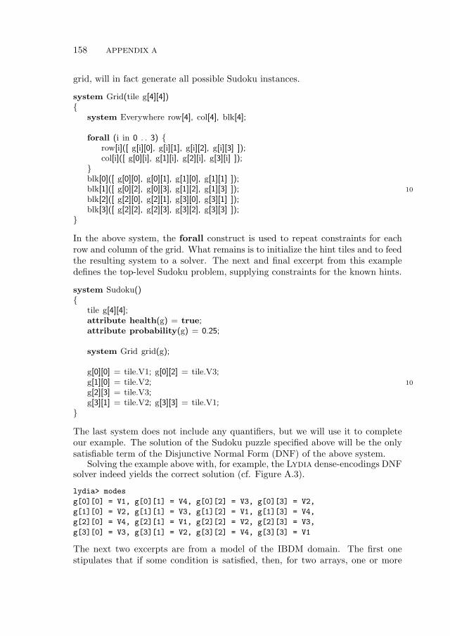
158 APPENDIX A
grid, will in fact generate all possible Sudoku instances.
system Grid(tile g[4][4])
system Everywhere row[4], col[4], blk[4];
forall (i in 0 . . 3) row[i]([ g[i][0], g[i][1], g[i][2], g[i][3] ]);col[i]([ g[0][i], g[1][i], g[2][i], g[3][i] ]);
blk[0]([ g[0][0], g[0][1], g[1][0], g[1][1] ]);blk[1]([ g[0][2], g[0][3], g[1][2], g[1][3] ]); 10
blk[2]([ g[2][0], g[2][1], g[3][0], g[3][1] ]);blk[3]([ g[2][2], g[2][3], g[3][2], g[3][3] ]);
In the above system, the forall construct is used to repeat constraints for eachrow and column of the grid. What remains is to initialize the hint tiles and to feedthe resulting system to a solver. The next and final excerpt from this exampledefines the top-level Sudoku problem, supplying constraints for the known hints.
system Sudoku()
tile g[4][4];attribute health(g) = true;attribute probability(g) = 0.25;
system Grid grid(g);
g[0][0] = tile.V1; g[0][2] = tile.V3;g[1][0] = tile.V2; 10
g[2][3] = tile.V3;g[3][1] = tile.V2; g[3][3] = tile.V1;
The last system does not include any quantifiers, but we will use it to completeour example. The solution of the Sudoku puzzle specified above will be the onlysatisfiable term of the Disjunctive Normal Form (DNF) of the above system.
Solving the example above with, for example, the Lydia dense-encodings DNFsolver indeed yields the correct solution (cf. Figure A.3).
lydia> modes
g[0][0] = V1, g[0][1] = V4, g[0][2] = V3, g[0][3] = V2,
g[1][0] = V2, g[1][1] = V3, g[1][2] = V1, g[1][3] = V4,
g[2][0] = V4, g[2][1] = V1, g[2][2] = V2, g[2][3] = V3,
g[3][0] = V3, g[3][1] = V2, g[3][2] = V4, g[3][3] = V1
The next two excerpts are from a model of the IBDM domain. The first onestipulates that if some condition is satisfied, then, for two arrays, one or more

PREDICATES 159
elements of each array should assume a certain value6.
if ((primaryRingGear = ringGear.forceLatching) or
(primaryRingGear = ringGear.forceUnlatching)) exists (i in 0 . . 11)
(primaryGearBoxState[i] = gearBoxState.jammed) or
(primaryLatchState[i] = latchState.jammed);
Finally, we illustrate the workings of the forall construct with one more examplefrom the IBDM domain. In this excerpt we couple a dozen of gear boxes to adozen of structural latch assemblies (these are all systems which share variables).
forall (i in 0 . . 11) gearBox[i](primaryGearBoxState[i], . . . , latchAssemblySecondaryCrank[i]);structuralLatchAssembly[i](primaryLatchState[i], . . . , latchRoller[i]);
6The intended meaning of the model is that an increased force when moving the primary orsecondary ring gears implies the existence of a gear box (there are twelve gear-boxes driven bythe two ring gears) or a latch which is mechanically jammed.

160 APPENDIX A

Appendix BCase Study: ADAPT EPS
In this appendix we demonstrate the applicability of Lydia/Safari to real-worldapplications, such as the diagnosis of the Electrical Power System (EPS) testbedin the ADAPT lab at NASA Ames Research Center [Poll et al., 2007].
ADAPT EPS has been used for the evaluation of the engineering and ap-plication aspects of diagnosis at the First International Diagnostic Competition(DXC’09) [Kurtoglu et al., 2009]. Lydia/Safari competed with twelve other Di-agnostic Algorithms (DAs) (model-based or not); many of those DAs optimizingone or more of the nine diagnostic metrics computed by the organizers.
Section B.1 offers of a description of ADAPT EPS and the diagnostic scenariosfrom which we have obtained observation vectors. Section B.2 describes the Lydia
ADAPT EPS model and can be used as a guideline for building models of electricalsystems. Section B.3 presents experiments and comparison to other DXC’09 DAs.
B.1 System Overview
The ADAPT EPS testbed provides a means for evaluating DAs through the con-trolled insertion of faults in repeatable failure scenarios. The EPS testbed incor-porates low-cost Commercial Off-The-Shelf (COTS) components connected in asystem topology that provides the functions typical of aerospace vehicle electricalpower systems: energy conversion/generation (battery chargers), energy storage(three sets of lead-acid batteries), power distribution (two inverters, several re-lays, circuit breakers, and loads) and power management (command, control, anddata acquisition).
The EPS delivers Alternating Current (AC) and Direct Current (DC) power toloads, which in an aerospace vehicle could include subsystems such as the avionics,propulsion, life support, environmental controls, and science payloads. A dataacquisition and control system commands the testbed into different configurations
161
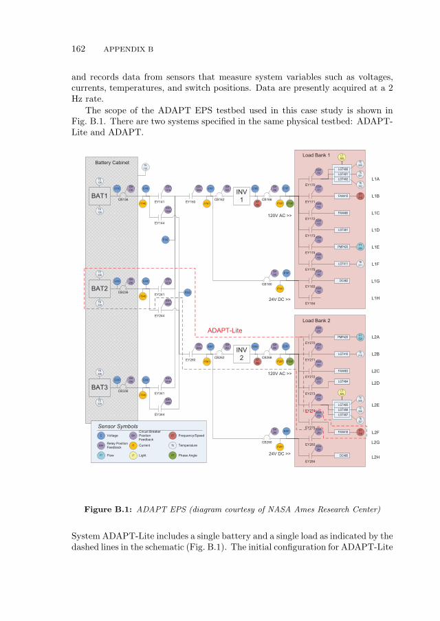
162 APPENDIX B
and records data from sensors that measure system variables such as voltages,currents, temperatures, and switch positions. Data are presently acquired at a 2Hz rate.
The scope of the ADAPT EPS testbed used in this case study is shown inFig. B.1. There are two systems specified in the same physical testbed: ADAPT-Lite and ADAPT.
E265
ST
265
CB136
CB236
CB336
CB266
CB166
ESH
170
EY160
ESH
160AE161
IT161
E165
ST
165
EY171
E167
IT167
ESH
171
EY172
ESH
172
EY170
EY174
ESH
174
EY175
ESH
175
EY173
ESH
173
EY183
ESH
183
EY184
ESH
184
L1A
L1B
L1C
L1D
L1E
L1F
L1G
L1H
Load Bank 1
120V AC >>
24V DC >>
Battery CabinetTE
133
BAT1
TE
128
E135
EY141
E140
EY144
IT140
ESH
141A
ESH
144ATE
129
ISH
136
ISH
162
CB162
ISH
166
ISH
180
CB180
ESH
270
EY260
ESH
260AE261
IT261EY271
E267
IT267
ESH
271
EY272
ESH
272
EY270
EY274
ESH
274
EY275
ESH
275
EY273
ESH
273
EY283
ESH
283
EY284
ESH
284
L2A
L2B
L2C
L2D
L2E
L2F
L2G
L2H
Load Bank 2
120V AC >>
24V DC >>
ISH
262
CB262
ISH
266
ISH
280
CB280
BAT2
TE
228
E235
EY241
E240
EY244
IT240
ESH
241A
ESH
244ATE
229
ISH
236
BAT3
TE
328
E335
EY341
E340
EY344
IT340
ESH
341A
ESH
344ATE
329
ISH
336
E142
E242
XT167
XT267
IT181
IT281
TE
500
TE
501
TE
502
LT
500
TE
505
TE
506
TE
507
LT
505
ST
515
FT
525
TE
511
FT
520
TE
510
ST
516
LGT400
LGT401
LGT402
LGT405
LGT406
LGT407
FAN415
FAN480
LGT481
PMP425
LGT411
DC482
PMP420
LGT410
FAN483
LGT484
FAN416
DC485
E181
E281
INV
1
INV
2
ADAPT-Lite
ESH
ISHE
IT
FT LT
ST
TE
XT
Voltage
Relay Position
Feedback
Circuit Breaker
Position
Feedback
Current
Flow Light
Frequency/Speed
Temperature
Phase Angle
Sensor Symbols
Figure B.1: ADAPT EPS (diagram courtesy of NASA Ames Research Center)
System ADAPT-Lite includes a single battery and a single load as indicated by thedashed lines in the schematic (Fig. B.1). The initial configuration for ADAPT-Lite

SYSTEM OVERVIEW 163
data has all relays and circuit breakers closed and no nominal mode changes arecommanded during the scenarios. Hence, any noticeable changes in sensor valuesmay be correctly attributed to faults injected into the scenarios. Furthermore,ADAPT-Lite is restricted to single faults.
Table B.1: ADAPT and ADAPT-Lite differences
Aspect ADAPT-Lite ADAPT
|COMPS| 37 173# of modes 93 430relays initially closed opencircuit-breakers initially closed closednominal mode changes no yesmultiple faults no yes
System ADAPT includes all batteries and loads in the EPS. The initial configu-ration for ADAPT has all relays open and nominal mode changes are commandedduring the scenarios. The commanded configuration changes result in adjustmentsto sensor values as well as transients which are nominal and not indicative of in-jected faults, in contrast to ADAPT-Lite. Finally, multiple faults may be injectedin ADAPT. The differences between ADAPT-Lite and ADAPT are summarizedin Table B.1.
ADAPT supports the repeatable injection of faults into the system in threeways:
Hardware-Induced Faults: These faults are physically injected at the testbedhardware. A simple example is tripping a circuit breaker using the manualthrow bars. Another is using the power toggle switch to turn off an inverter.Faults may also be introduced in the loads attached to the EPS. For example,the valve can be closed slightly to vary the back pressure on the pump andreduce the flow rate.
Software-Induced Faults: In addition to hardware faults, ADAPT supportssoftware simulation of faulty behavior. Software fault injection includes oneor more of the following: (1) sending commands to the testbed that are notintended for nominal operations; (2) blocking commands sent to the testbed;and (3) altering the testbed sensor data.
Real Faults: In addition the aforementioned two methods, real faults may beinjected into the system by using actual faulty components. A simple ex-ample includes a burned out light bulb. This method of fault injection wasnot used in this study.
For results presented in this case study, only abrupt discrete (change in operat-ing mode of component) and parametric (step change in parameter value) faults
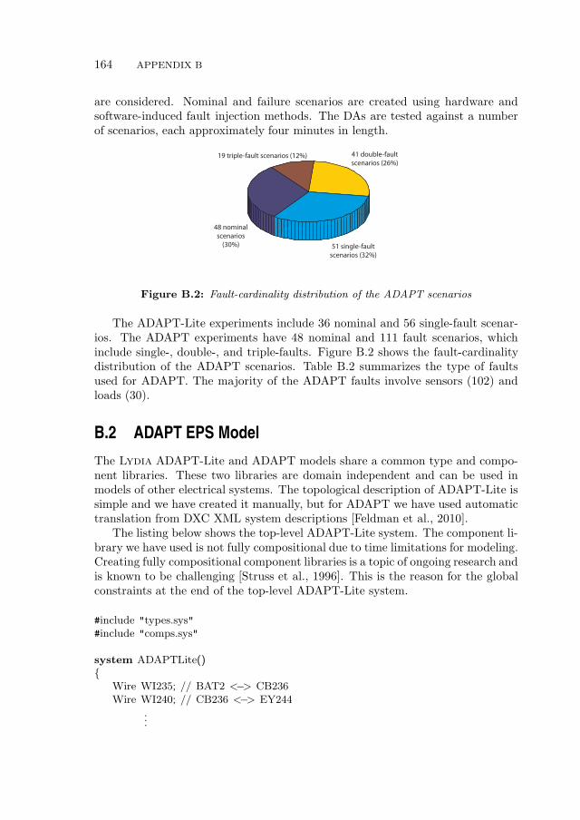
164 APPENDIX B
are considered. Nominal and failure scenarios are created using hardware andsoftware-induced fault injection methods. The DAs are tested against a numberof scenarios, each approximately four minutes in length.
41 double-faultscenarios (26%)
51 single-faultscenarios (32%)
19 triple-fault scenarios (12%)
48 nominalscenarios
(30%)
Figure B.2: Fault-cardinality distribution of the ADAPT scenarios
The ADAPT-Lite experiments include 36 nominal and 56 single-fault scenar-ios. The ADAPT experiments have 48 nominal and 111 fault scenarios, whichinclude single-, double-, and triple-faults. Figure B.2 shows the fault-cardinalitydistribution of the ADAPT scenarios. Table B.2 summarizes the type of faultsused for ADAPT. The majority of the ADAPT faults involve sensors (102) andloads (30).
B.2 ADAPT EPS Model
The Lydia ADAPT-Lite and ADAPT models share a common type and compo-nent libraries. These two libraries are domain independent and can be used inmodels of other electrical systems. The topological description of ADAPT-Lite issimple and we have created it manually, but for ADAPT we have used automatictranslation from DXC XML system descriptions [Feldman et al., 2010].
The listing below shows the top-level ADAPT-Lite system. The component li-brary we have used is not fully compositional due to time limitations for modeling.Creating fully compositional component libraries is a topic of ongoing research andis known to be challenging [Struss et al., 1996]. This is the reason for the globalconstraints at the end of the top-level ADAPT-Lite system.
#include "types.sys"#include "comps.sys"
system ADAPTLite()
Wire WI235; // BAT2 <−> CB236Wire WI240; // CB236 <−> EY244
...
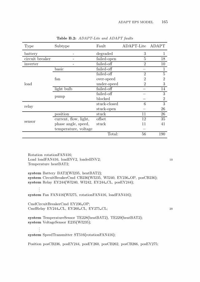
ADAPT EPS MODEL 165
Table B.2: ADAPT-Lite and ADAPT faults
Type Subtype Fault ADAPT-Lite ADAPT
battery - degraded 3 1circuit breaker - failed-open 5 18inverter - failed-off 2 10
load
basic failed-off − 1
fanfailed-off 2 5over-speed 2 2under-speed 2 3
light bulb failed-off − 14
pumpfailed-off − 3blocked − 2
relaystuck-closed 6 3stuck-open − 26
sensor
position stuck 11 26current, flow, light, offset 12 35phase angle, speed, stuck 11 41temperature, voltage −
Total: 56 190
Rotation rotationFAN416;Load loadFAN416, loadINV2, loadedINV2; 10
Temperature heatBAT2;
system Battery BAT2(WI235, heatBAT2);system CircuitBreakerCmd CB236(WI235, WI240, EY236 OP, posCB236);system Relay EY244(WI240, WI242, EY244 CL, posEY244);
...system Fan FAN416(WI275, rotationFAN416, loadFAN416);
CmdCircuitBreakerCmd EY236 OP;CmdRelay EY244 CL, EY260 CL, EY275 CL; 20
system TemperatureSensor TE228(heatBAT2), TE229(heatBAT2);system VoltageSensor E235(WI235);
...system SpeedTransmitter ST516(rotationFAN416);
Position posCB236, posEY244, posEY260, posCB262, posCB266, posEY275;
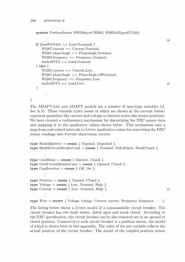
166 APPENDIX B
system PositionSensor ISH236(posCB236), ESH244A(posEY244);
... 30
if (loadFAN416 == Load.Nominal) WI267.current == Current.Nominal;
WI267.phaseAngle == PhaseAngle.Nominal;WI265.frequency == Frequency.Nominal;
loadedINV2 == Load.Nominal;
else WI267.current == Current.Low;
WI267.phaseAngle == PhaseAngle.OffNominal;
WI265.frequency == Frequency.Low;loadedINV2 == Load.Low; 40
...
The ADAPT-Lite and ADAPT models use a number of user-type variables (cf.Sec A.3). These variable types (some of which are shown in the excerpt below)represent quantities like current and voltage or discrete states like sensor positions.We have created a rudimentary mechanism for discretizing the DXC sensor dataand mapping it to the qualitative values shown below. This mechanism uses amap from real-valued intervals to Lydia qualitative values for converting the DXCsensor readings into Safari observation vectors.
type HealthBattery = enum Nominal, Degraded ;type HealthCircuitBreakerCmd = enum Nominal, FailedOpen, StuckClosed ;
...type CmdRelay = enum Opened, Closed ;
type CmdCircuitBreakerCmd = enum Opened, Closed ;
type CmdInverter = enum Off, On ;
...
type Position = enum Opened, Closed ;type Voltage = enum Low, Nominal, High ;
type Current = enum Low, Nominal, High ; 10
...
type Wire = struct Voltage voltage, Current current, Frequency frequency, · · · ;
The listing below shows a Lydia model of a commandable circuit breaker. Thecircuit breaker has two fault states: failed open and stuck closed. According tothe DXC specification, the circuit breaker can be also remotely set in an opened orclosed position. Connected to each circuit breaker is a position sensor, the modelof which is shown later in this appendix. The value of the pos variable reflects theactual position of the circuit breaker. The model of the coupled position sensor

ADAPT EPS MODEL 167
allows Safari to infer the sensor health by comparing the value of pos to theobserved sensor reading.
system CircuitBreakerCmd(Wire i, o, CmdCircuitBreakerCmd commanded,Position pos)
HealthCircuitBreakerCmd h;
attribute health(h) = cond (h) (HealthCircuitBreakerCmd.Nominal −> true;HealthCircuitBreakerCmd.FailedOpen −> false;
HealthCircuitBreakerCmd.StuckClosed −> false
); 10
attribute probability(h) = cond (h) (HealthCircuitBreakerCmd.Nominal −> 0.8;HealthCircuitBreakerCmd.FailedOpen −> 0.1;
HealthCircuitBreakerCmd.StuckClosed −> 0.1);
switch (h) HealthCircuitBreakerCmd.Nominal −>
switch (commanded) 20
CmdCircuitBreakerCmd.Closed −>
pos = Position.Closed; o.voltage = i.voltage;
CmdCircuitBreakerCmd.Opened −>
pos = Position.Opened;
30
HealthCircuitBreakerCmd.FailedOpen −>
pos = Position.Opened;
HealthCircuitBreakerCmd.StuckClosed −>
pos = Position.Closed; o.voltage = i.voltage;
40
The ADAPT EPS uses two off-the-shelf inverters. There is an inverter in eachADAPT DC or AC circuit. In the listing below we show a Lydia model of aninverter. We have introduced the loadOut variable because the inverters switch
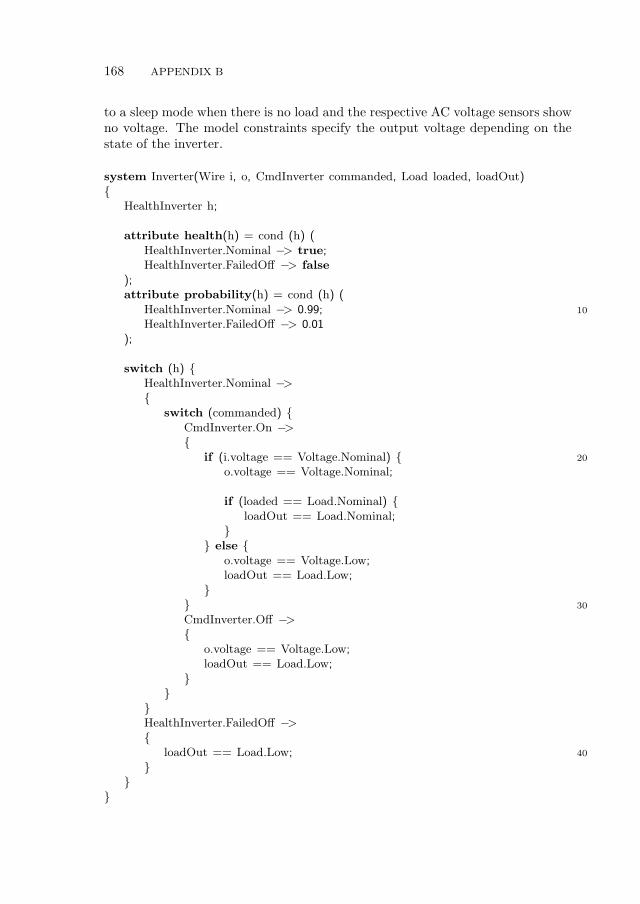
168 APPENDIX B
to a sleep mode when there is no load and the respective AC voltage sensors showno voltage. The model constraints specify the output voltage depending on thestate of the inverter.
system Inverter(Wire i, o, CmdInverter commanded, Load loaded, loadOut)
HealthInverter h;
attribute health(h) = cond (h) (HealthInverter.Nominal −> true;HealthInverter.FailedOff −> false
);attribute probability(h) = cond (h) (
HealthInverter.Nominal −> 0.99; 10
HealthInverter.FailedOff −> 0.01);
switch (h) HealthInverter.Nominal −>
switch (commanded)
CmdInverter.On −>
if (i.voltage == Voltage.Nominal) 20
o.voltage == Voltage.Nominal;
if (loaded == Load.Nominal) loadOut == Load.Nominal;
else
o.voltage == Voltage.Low;loadOut == Load.Low;
30
CmdInverter.Off −>
o.voltage == Voltage.Low;loadOut == Load.Low;
HealthInverter.FailedOff −>
loadOut == Load.Low; 40
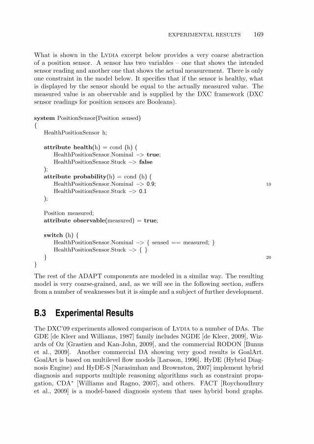
EXPERIMENTAL RESULTS 169
What is shown in the Lydia excerpt below provides a very coarse abstractionof a position sensor. A sensor has two variables – one that shows the intendedsensor reading and another one that shows the actual measurement. There is onlyone constraint in the model below. It specifies that if the sensor is healthy, whatis displayed by the sensor should be equal to the actually measured value. Themeasured value is an observable and is supplied by the DXC framework (DXCsensor readings for position sensors are Booleans).
system PositionSensor(Position sensed)
HealthPositionSensor h;
attribute health(h) = cond (h) (HealthPositionSensor.Nominal −> true;
HealthPositionSensor.Stuck −> false
);
attribute probability(h) = cond (h) (HealthPositionSensor.Nominal −> 0.9; 10
HealthPositionSensor.Stuck −> 0.1
);
Position measured;
attribute observable(measured) = true;
switch (h) HealthPositionSensor.Nominal −> sensed == measured; HealthPositionSensor.Stuck −>
20
The rest of the ADAPT components are modeled in a similar way. The resultingmodel is very coarse-grained, and, as we will see in the following section, suffersfrom a number of weaknesses but it is simple and a subject of further development.
B.3 Experimental Results
The DXC’09 experiments allowed comparison of Lydia to a number of DAs. TheGDE [de Kleer and Williams, 1987] family includes NGDE [de Kleer, 2009], Wiz-ards of Oz [Grastien and Kan-John, 2009], and the commercial RODON [Bunuset al., 2009]. Another commercial DA showing very good results is GoalArt.GoalArt is based on multilevel flow models [Larsson, 1996]. HyDE (Hybrid Diag-nosis Engine) and HyDE-S [Narasimhan and Brownston, 2007] implement hybriddiagnosis and supports multiple reasoning algorithms such as constraint propa-gation, CDA∗ [Williams and Ragno, 2007], and others. FACT [Roychoudhuryet al., 2009] is a model-based diagnosis system that uses hybrid bond graphs.
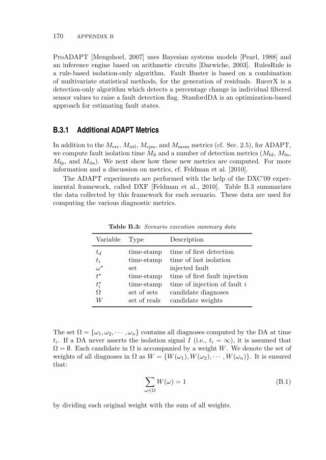
170 APPENDIX B
ProADAPT [Mengshoel, 2007] uses Bayesian systems models [Pearl, 1988] andan inference engine based on arithmetic circuits [Darwiche, 2003]. RulesRule isa rule-based isolation-only algorithm. Fault Buster is based on a combinationof multivariate statistical methods, for the generation of residuals. RacerX is adetection-only algorithm which detects a percentage change in individual filteredsensor values to raise a fault detection flag. StanfordDA is an optimization-basedapproach for estimating fault states.
B.3.1 Additional ADAPT Metrics
In addition to theMerr, Mutl, Mcpu, andMmem metrics (cf. Sec. 2.5), for ADAPT,we compute fault isolation time Mfi and a number of detection metrics (Mfd, Mfn,Mfp, and Mda). We next show how these new metrics are computed. For moreinformation and a discussion on metrics, cf. Feldman et al. [2010].
The ADAPT experiments are performed with the help of the DXC’09 exper-imental framework, called DXF [Feldman et al., 2010]. Table B.3 summarizesthe data collected by this framework for each scenario. These data are used forcomputing the various diagnostic metrics.
Table B.3: Scenario execution summary data
Variable Type Description
td time-stamp time of first detectionti time-stamp time of last isolationω⋆ set injected faultt⋆ time-stamp time of first fault injectiont⋆i time-stamp time of injection of fault iΩ set of sets candidate diagnosesW set of reals candidate weights
The set Ω = ω1, ω2, · · · , ωn contains all diagnoses computed by the DA at timeti. If a DA never asserts the isolation signal I (i.e., ti = ∞), it is assumed thatΩ = ∅. Each candidate in Ω is accompanied by a weight W . We denote the set ofweights of all diagnoses in Ω as W = W (ω1),W (ω2), · · · ,W (ωn). It is ensuredthat:
∑
ω∈Ω
W (ω) = 1 (B.1)
by dividing each original weight with the sum of all weights.

EXPERIMENTAL RESULTS 171
Fault Detection Time
The fault detection time (the reaction time for a diagnostic engine to detect ananomaly) is directly measured as:
Mfd = td (B.2)
The fault detection time is reported in milliseconds and is computed only fornon-nominal scenarios for which a DA asserts the time detection signal at leastonce.
False Negative Scenario
The false negative scenario metric measures whether a fault is missed by a diag-nostic algorithm and is defined as:
Mfn =
1, if td =∞0, otherwise
(B.3)
False Positive Scenario
The false positive scenario metric penalizes DAs which announce spurious faultsand is defined as:
Mfp =
1, if td < t⋆
0, otherwise(B.4)
where t⋆ = ∞ for nominal scenarios (i.e., scenarios during which no fault isinjected).
Note that the above two metrics (Mfn and Mfp) are computed for each scenarioand their computation is based on the times of injecting and announcing thefault. We also have false negative and false positive components in the contextof individual diagnostic candidates (recall that a DA sends a set of diagnosticcandidates at isolation time) which we have discussed in Sec. 2.5.
Scenario Detection Accuracy
The scenario detection accuracy metric is computed from Mfn and Mfp:
Mda = 1−max(Mfn,Mfp) (B.5)
Mda is 1 if the scenario is true positive or true negative and 0 otherwise (equiv-alently, Mda = 0 if Mfn = 1 or Mfp = 1, and Mda = 1 otherwise). Mda splitsall scenarios into “true” and “false”. Incorrect scenarios are further classified intofalse positive (Mfp) and false negative (Mfn). Correct scenarios are true positiveif there are injected faults and true negative otherwise (the latter separation intotrue positives and true negatives is rarely of practical importance).
172 APPENDIX B
Fault Isolation Time
Consider an injected fault ω⋆ = c1, c2, · · · , cn with the individual componentfaults injected at times T ⋆ = 〈t⋆1, t⋆2, · · · , t⋆n〉. Next, from the isolation signal,we construct a sequence of isolation times for each component. This sequencecontaining time-stamps of rising edges of the isolation signal is denoted as Ti
(Ti = 〈t1, t2, · · · , tn〉). Note that t⋆k < ti for 1 ≤ k ≤ n. The fault isolation timeis then computed as:
Mfi =1
n
n∑
k=1
tk − t⋆k (B.6)
If there is no isolation for specific fault (i.e., a fault is missed) then there is nodifference tk − t⋆k computed for that fault. E.g., if in a fault ω⋆ = 〈c1, c2, c3〉, c1is isolated, c2 is not, and c3 is; the isolation time t2 − t⋆2 is undefined and notincluded in the average (n = 2).
The fault isolation time is reported in milliseconds and is computed only fornon-nominal scenarios for which a DA asserts the time isolation signal at leastonce.
System Metrics
The “per system”metrics Mfd, Mfn, Mfp, and Mda are defined in a way analogousto Mutl (cf. Sec. 2.5.5).
Note that Mfn, Mfp, and Mda are called false negative scenario, false positivescenario and scenario detection accuracy, respectively. The analogous “per sys-tem” metrics Mfn, Mfp, and Mda are called false negative rate, false positive rate,and detection accuracy. Mda, for example, represents the ratio of the number ofcorrectly classified cases to the total number of cases. The latter “per system”metrics (Mfn, Mfp, and Mda) are equivalent to the ones in Kurtoglu et al. [2009].In this paper we first define each metric “per scenario” and then “per system”.
B.3.2 Benchmarking Results
The DA benchmarking results for ADAPT-Lite are shown in Table B.4, withgraphical depictions of some of the tabular data presented in Fig. B.3. No DAdominates over all metrics used in benchmarking; nine of eleven DAs tested arebest or second best with respect to at least one of the metrics.
Lydia is second in memory consumption and the average CPU time spentper scenario is approx. 1.5 s. With ADAPT-Lite, Lydia/Safari show low falsepositive and false negative rate but large number of classification errors. Thereason for that is the ambiguity (lack of constraints) in the ADAPT-Lite model.Lydia does not discern between fault-detection and fault-isolation times, hence itis one of the fastest algorithms in these two metrics. One way to reduce the largenumber of classification errors without modifying the model is to use Fractal.
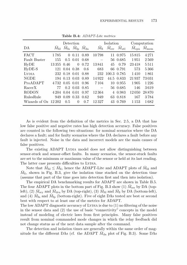
EXPERIMENTAL RESULTS 173
Table B.4: ADAPT-Lite metrics
Detection Isolation ComputationDA Mfd Mfn Mfp Mda Mfi Merr Mutl Mcpu Mmem
FACT 1 785 0 0.11 0.89 10 798 11 0.975 15 815 4 271Fault Buster 155 0.5 0.01 0.68 − 56 0.685 1 951 2 569HyDE 13 355 0.46 0 0.72 13 841 45 0.79 23 418 5 511HyDE-S 121 0.04 0.38 0.6 683 66 0.791 573 5 366Lydia 232 0.18 0.01 0.88 232 100.3 0.785 1 410 1 861NGDE 194 0.13 0.03 0.89 14 922 44.5 0.833 21 937 73 031ProADAPT 4 732 0.05 0.01 0.96 7 104 10 0.955 1 905 1 226RacerX 77 0.2 0.03 0.85 − 56 0.685 146 3 619RODON 4 204 0.04 0.01 0.97 12 364 4 0.983 12 050 28 870RulesRule 949 0.09 0.33 0.62 949 63 0.818 167 3 784Wizards of Oz 12 202 0.5 0 0.7 12 327 43 0.769 1 153 1 682
As is evident from the definition of the metrics in Sec. 2.5, a DA that haslow false positive and negative rates has high detection accuracy. False positivesare counted in the following two situations: for nominal scenarios where the DAdeclares a fault; and for faulty scenarios where the DA declares a fault before anyfault is injected. Noise in the data and incorrect models are the main causes offalse positives.
The existing ADAPT Lydia model does not allow distinguishing betweensensor-stuck and sensor-offset faults. In many scenarios, the sensor-stuck faultsare set to the minimum or maximum value of the sensor or held at its last reading.The latter case presents difficulties to Lydia.
Note that Mfd ≤ Mfi, hence the ADAPT-Lite and ADAPT plots of Mfd andMfi, shown in Fig. B.3, give the isolation time stacked on the detection time(assume that part of the time goes into detection first and then into isolation).
The empirical DA benchmarking results for ADAPT are shown in Table B.5.The four ADAPT plots in the bottom part of Fig. B.3 show (1) Merr by DA (top-left), (2) Msry and Mdru by DA (top-right), (3) Mfd and Mfi by DA (bottom-left),and (4) Mfn and Mfp (bottom-right). Five of eight DAs tested are best or secondbest with respect to at least one of the metrics for ADAPT.The low ADAPT diagnostic accuracy of Lydia is due to (1) no filtering of the noisein the sensor data and (2) the use of basic “connectivity” concepts in the modelinstead of modeling of electric laws from first principles. Many false positivesresult from nominal commanded mode changes in which the relay feedback didnot change status as of the next data sample after the command.
The detection and isolation times are generally within the same order of mag-nitude for the different DAs (cf. the ADAPT Mda plot of Fig. B.3). Some DAs
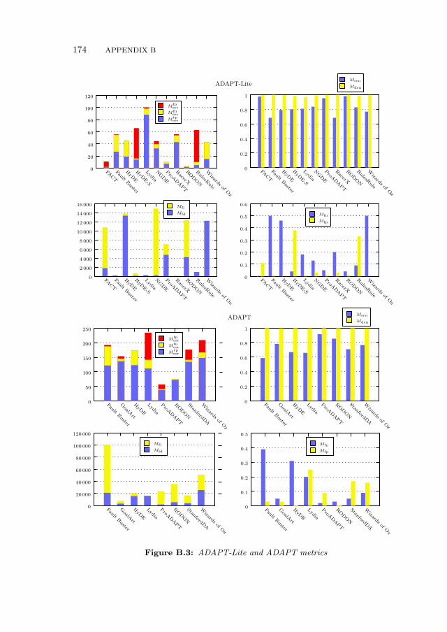
174 APPENDIX B
Mfn
Mfp
Mfi
Mfd
Msru
Mdru
Mfperr
Mfnerr
Mtperr
Mfperr
Mfnerr
Mtperr
Msru
MdruADAPT
ADAPT-Lite
Mfn
Mfp
Mfi
Mfd
0
2 000
4 000
6 000
8 000
10 000
12 000
14 000
16 000
0
0.2
0.4
0.6
0.8
1
0
0.1
0.2
0.3
0.4
0.5
0.6
FACT
FaultBuster
HyD
E
HyD
E-S
Lydia
NGDE
ProA
DAPT
RacerX
RODON
RulesR
ule
Wizards
ofOz
0
20
40
60
80
100
120
FACT
FaultBuster
HyD
E
HyD
E-S
Lydia
NGDE
ProA
DAPT
RacerX
RODON
RulesR
ule
Wizards
ofOz
FACT
FaultBuster
HyD
E
HyD
E-S
Lydia
NGDE
ProA
DAPT
RacerX
RODON
RulesR
ule
Wizards
ofOz
FACT
FaultBuster
HyD
E
HyD
E-S
Lydia
NGDE
ProA
DAPT
RacerX
RODON
RulesR
ule
Wizards
ofOz
0
0.1
0.2
0.3
0.4
0.5
FaultBuster
GoalA
rt
HyD
E
Lydia
ProA
DAPT
RODON
StanfordDA
Wizards
ofOz
0
0.2
0.4
0.6
0.8
1
FaultBuster
GoalA
rt
HyD
E
Lydia
ProA
DAPT
RODON
StanfordDA
Wizards
ofOz
0
20 000
40 000
60 000
80 000
100 000
120 000
FaultBuster
GoalA
rt
HyD
E
Lydia
ProA
DAPT
RODON
StanfordDA
Wizards
ofOz
0
50
100
150
200
250
FaultBuster
GoalA
rt
HyD
E
Lydia
ProA
DAPT
RODON
StanfordDA
Wizards
ofOz
Figure B.3: ADAPT-Lite and ADAPT metrics

SUMMARY 175
Table B.5: ADAPT metrics results
Detection Isolation ComputationDA Mfd Mfn Mfp Mda Mfi Merr Mutl Mcpu Mmem
Fault Buster 21 255 0.39 0.03 0.70 100 292 193 0.587 10 051 7 119GoalArt 3 268 0.05 0.03 0.93 7 805 154 0.776 149 6 784HyDE 15 612 0.31 0 0.79 20 114 174.3 0.668 28 807 19 135Lydia 16 135 0.2 0.25 0.62 16 135 234.9 0.653 5 715 3 412ProADAPT 1 743 0.02 0.09 0.90 23 544 57 0.915 4 260 778RODON 5 543 0.03 0 0.98 35 792 75.6 0.853 85 331 31 459StanfordDA 3 826 0.05 0.17 0.79 16 816 176.6 0.706 1 012 2 213Wizards of Oz 25 695 0.09 0.16 0.77 50 980 209.2 0.76 17 111 3 390
have isolation times that are similar to their detection times while others showisolation times that are much greater than the detection times. This could reflectdifferences in reasoning strategies or differences in policies for when to declare anisolation based on accumulated evidence.
The left plots of Figure B.4 show detection accuracy for all DAs by faulttype for ADAPT-Lite and ADAPT. In general, Mda is not very sensitive to thecomponent type, except in the case of load and sensor faults where it is lower. Thedata on the battery detection accuracy is not representative due to the limitednumber of fault scenarios containing battery faults (cf. Table B.2). It is visiblefrom Fig. B.4 that Lydia has lower diagnostic accuracy for sensor and load faults.The latter is due to the limited modeling of loads.
The right plots of Figure B.4 show classification errors for all DAs by faulttype for ADAPT-Lite and ADAPT. The number of classification errors in sensorfault scenarios is quite high. Part of the reason, of course, is simply that there aremore scenarios involving sensors that other fault types (cf. Table B.2). Anotherreason is due to the fact that most DAs reported either stuck or offset consistentlyor they reported both with equal weight.
The total number of classification errors is significantly larger in ADAPT com-pared to ADAPT-Lite (to see this, multiply Merr by the number of fault modesin each system). One of the reasons is because of the presence of multiple faults.
B.4 Summary
In this appendix we have shown the use of Lydia/Safari for solving the ADAPTEPS diagnostic challenge. The results demonstrate that the Lydia/Safari ap-proach is applicable to models beyond digital circuits. Safari has outperformedmany of the DAs in the ADAPT-Lite challenge. We have identified modeling as
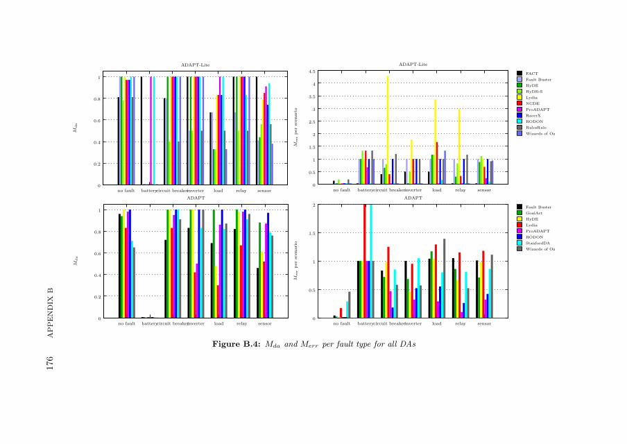
176
AP
PE
ND
IXB
Fault Buster
GoalArt
HyDE
Lydia
ProADAPT
RODON
StanfordDA
Wizards of Oz
FACT
Fault Buster
HyDE
HyDE-S
Lydia
NGDE
ProADAPT
RacerX
RODON
RulesRule
Wizards of Oz
0
0.2
0.4
0.6
0.8
1
no fault batterycircuit breakerinverter load relay sensor
ADAPT-Lite
0
0.2
0.4
0.6
0.8
1
no fault batterycircuit breakerinverter load relay sensor
ADAPT
0
0.5
1
1.5
2
no fault batterycircuit breakerinverter load relay sensor
ADAPT
0
0.5
1
1.5
2
2.5
3
3.5
4
4.5
no fault batterycircuit breakerinverter load relay sensor
ADAPT-Lite
Mda
Mda
Merr
per
scenari
oM
err
per
scenari
o
Figure B.4: Mda and Merr per fault type for all DAs

SUMMARY 177
the main reason for the worse ADAPT results. The average running time of Sa-
fari for diagnosing ADAPT, a system with 723 variables and 1567 clauses, wasbelow 6 s which makes Safari one of the fastest MBD algorithms. As a result ofthe coarse Lydia model, Safari has computed large diagnostic sets which lead toan average of 1.48 classification errors per scenario. This diagnostic uncertaintycan be improved by using the Fractal approach as illustrated in the appendixthat comes next.

178 APPENDIX B

Appendix CCase Study: Paper Input Module
In this appendix we demonstrate the applicability of Fractal to real-world ap-plications, such as the diagnosis of a Paper Input Module (PIM), part of a heavy-duty printer. We show that (1) Fractal computes intuitive results given thePIM model and an initial observation and (2) Fractal leads to a steep reduc-tion in the number of diagnoses even with very coarse-grained models and in thelack of prior failure probabilities.
C.1 System Overview
Before we describe the PIM we introduce a related printer modeling and diagnosisproject. Figure C.1 shows the Tightly Integrated Parallel Printer (TIPP) fixture,devised by the Palo Alto Research Center (PARC) and used for studying MBDtechniques and algorithms from, amongst others, planning, probing, testing, andcontrol theory.
The PIM is similar to the TIPP fixture but smaller in size, thus enabling thedevelopment of a higher-precision model. The PIM, as shown in Fig. C.2, is usedto supply paper to a printing module or to a finisher. Up to three PIM devicescan be chained to supply paper to the printing unit and one PIM can be placedbetween the printer and the finisher to insert blank pages when requested.
A PIM has four paper trays which are placed vertically and numbered 1 to4, starting from the top. Each tray can hold some amount of paper. The PIMhas its own power supply. It receives commands via a Controller-Area Network(CAN) bus. A command can instruct the PIM to separate a sheet from tray n,horizontally transport a sheet (from a chained tray or from a manual feed), etc.
The PIM uses compressed air to separate the sheets of paper. The air isprovided by an electrical fan. A dozen of solenoid valves (three per tray) controlthe air flow when a separation is requested. After a sheet of paper is separated,
179
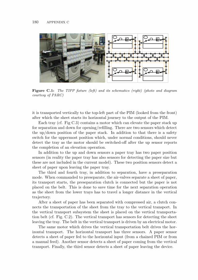
180 APPENDIX C
Figure C.1: The TIPP fixture (left) and its schematics (right) (photo and diagramcourtesy of PARC)
it is transported vertically to the top-left part of the PIM (looked from the front)after which the sheet starts its horizontal journey to the output of the PIM.
Each tray (cf. Fig C.3) contains a motor which can elevate the paper stack upfor separation and down for opening/refilling. There are two sensors which detectthe up/down position of the paper stack. In addition to that there is a safetyswitch for the uppermost position which, under normal conditions, should neverdetect the tray as the motor should be switched-off after the up sensor reportsthe completion of an elevation operation.
In addition to the up and down sensors a paper tray has two paper positionsensors (in reality the paper tray has also sensors for detecting the paper size butthese are not included in the current model). These two position sensors detect asheet of paper upon leaving the paper tray.
The third and fourth tray, in addition to separation, have a preseparationmode. When commanded to preseparate, the air-valves separate a sheet of paper,its transport starts, the preseparation clutch is connected but the paper is notplaced on the belt. This is done to save time for the next separation operationas the sheet from the lower trays has to travel a longer distance in the verticaltrajectory.
After a sheet of paper has been separated with compressed air, a clutch con-nects the transportation of the sheet from the tray to the vertical transport. Inthe vertical transport subsystem the sheet is placed on the vertical transporta-tion belt (cf. Fig. C.2). The vertical transport has sensors for detecting the sheetleaving the tray. The belt in the vertical transport is driven by an electrical motor.
The same motor which drives the vertical transportation belt drives the hor-izontal transport. The horizontal transport has three sensors. A paper sensordetects a sheet of paper fed to the horizontal input (from a chained PIM or froma manual feed). Another sensor detects a sheet of paper coming from the verticaltransport. Finally, the third sensor detects a sheet of paper leaving the device.
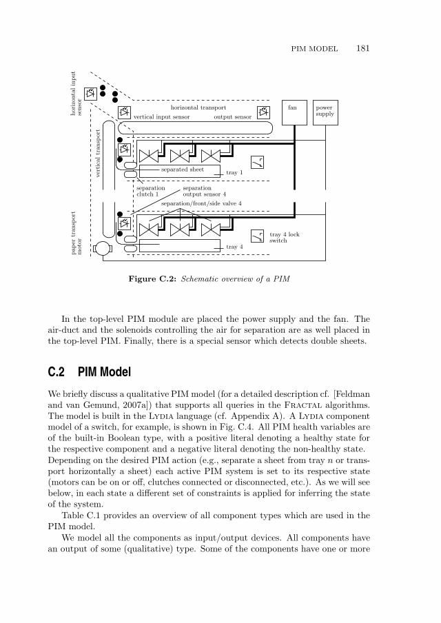
PIM MODEL 181
powersupply
ver
tica
ltr
ansp
ort
fan
horizo
nta
lin
put
horizontal transport
output sensor
senso
r
vertical input sensor
paper
transp
ort
moto
r
separated sheettray 1
tray 4
tray 4 lockswitch
separationoutput sensor 4
separationclutch 1
separation/front/side valve 4
Figure C.2: Schematic overview of a PIM
In the top-level PIM module are placed the power supply and the fan. Theair-duct and the solenoids controlling the air for separation are as well placed inthe top-level PIM. Finally, there is a special sensor which detects double sheets.
C.2 PIM Model
We briefly discuss a qualitative PIM model (for a detailed description cf. [Feldmanand van Gemund, 2007a]) that supports all queries in the Fractal algorithms.The model is built in the Lydia language (cf. Appendix A). A Lydia componentmodel of a switch, for example, is shown in Fig. C.4. All PIM health variables areof the built-in Boolean type, with a positive literal denoting a healthy state forthe respective component and a negative literal denoting the non-healthy state.Depending on the desired PIM action (e.g., separate a sheet from tray n or trans-port horizontally a sheet) each active PIM system is set to its respective state(motors can be on or off, clutches connected or disconnected, etc.). As we will seebelow, in each state a different set of constraints is applied for inferring the stateof the system.
Table C.1 provides an overview of all component types which are used in thePIM model.
We model all the components as input/output devices. All components havean output of some (qualitative) type. Some of the components have one or more
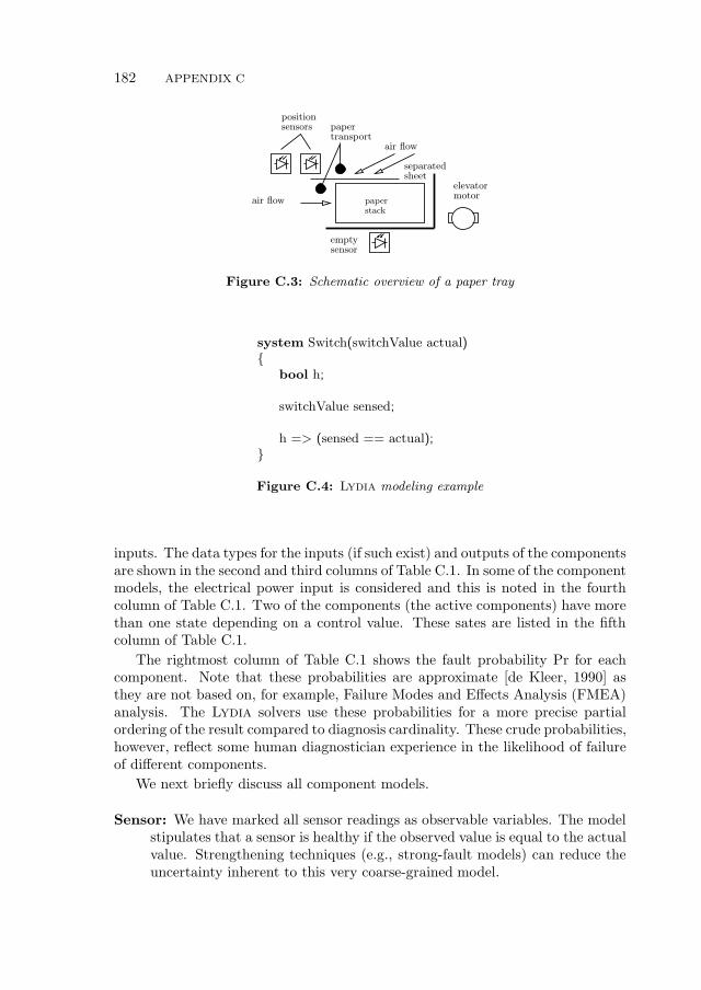
182 APPENDIX C
air flowmotor
stackpaper
emptysensor
elevatorsheetseparated
air flowtransportpapersensors
position
Figure C.3: Schematic overview of a paper tray
system Switch(switchValue actual)
bool h;
switchValue sensed;
h => (sensed == actual);
Figure C.4: Lydia modeling example
inputs. The data types for the inputs (if such exist) and outputs of the componentsare shown in the second and third columns of Table C.1. In some of the componentmodels, the electrical power input is considered and this is noted in the fourthcolumn of Table C.1. Two of the components (the active components) have morethan one state depending on a control value. These sates are listed in the fifthcolumn of Table C.1.
The rightmost column of Table C.1 shows the fault probability Pr for eachcomponent. Note that these probabilities are approximate [de Kleer, 1990] asthey are not based on, for example, Failure Modes and Effects Analysis (FMEA)analysis. The Lydia solvers use these probabilities for a more precise partialordering of the result compared to diagnosis cardinality. These crude probabilities,however, reflect some human diagnostician experience in the likelihood of failureof different components.
We next briefly discuss all component models.
Sensor: We have marked all sensor readings as observable variables. The modelstipulates that a sensor is healthy if the observed value is equal to the actualvalue. Strengthening techniques (e.g., strong-fault models) can reduce theuncertainty inherent to this very coarse-grained model.
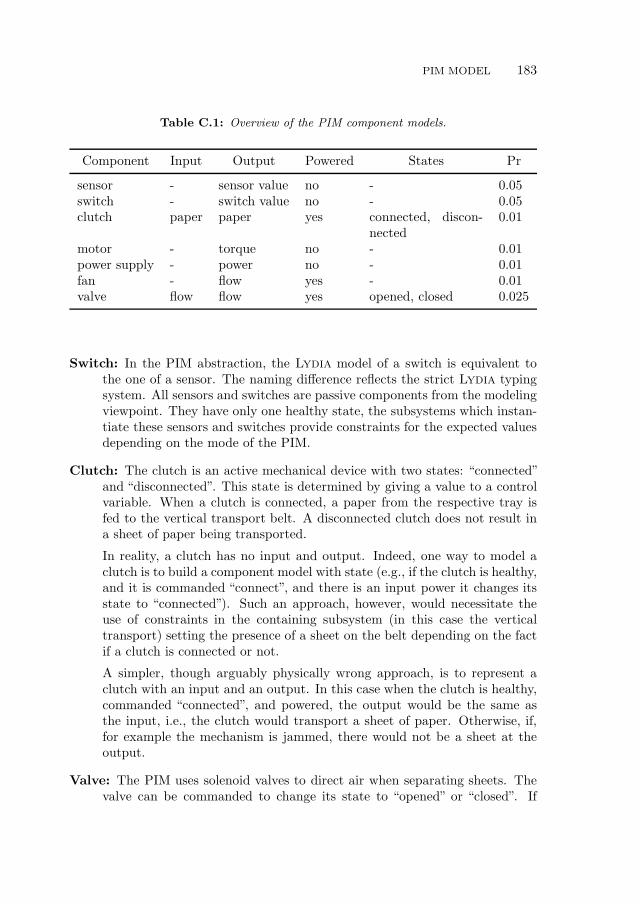
PIM MODEL 183
Table C.1: Overview of the PIM component models.
Component Input Output Powered States Pr
sensor - sensor value no - 0.05switch - switch value no - 0.05clutch paper paper yes connected, discon-
nected0.01
motor - torque no - 0.01power supply - power no - 0.01fan - flow yes - 0.01valve flow flow yes opened, closed 0.025
Switch: In the PIM abstraction, the Lydia model of a switch is equivalent tothe one of a sensor. The naming difference reflects the strict Lydia typingsystem. All sensors and switches are passive components from the modelingviewpoint. They have only one healthy state, the subsystems which instan-tiate these sensors and switches provide constraints for the expected valuesdepending on the mode of the PIM.
Clutch: The clutch is an active mechanical device with two states: “connected”and “disconnected”. This state is determined by giving a value to a controlvariable. When a clutch is connected, a paper from the respective tray isfed to the vertical transport belt. A disconnected clutch does not result ina sheet of paper being transported.
In reality, a clutch has no input and output. Indeed, one way to model aclutch is to build a component model with state (e.g., if the clutch is healthy,and it is commanded “connect”, and there is an input power it changes itsstate to “connected”). Such an approach, however, would necessitate theuse of constraints in the containing subsystem (in this case the verticaltransport) setting the presence of a sheet on the belt depending on the factif a clutch is connected or not.
A simpler, though arguably physically wrong approach, is to represent aclutch with an input and an output. In this case when the clutch is healthy,commanded “connected”, and powered, the output would be the same asthe input, i.e., the clutch would transport a sheet of paper. Otherwise, if,for example the mechanism is jammed, there would not be a sheet at theoutput.
Valve: The PIM uses solenoid valves to direct air when separating sheets. Thevalve can be commanded to change its state to “opened” or “closed”. If

184 APPENDIX C
the valve is healthy and it is commanded open, then the valve’s input flowshould equal the valve’s output flow. Otherwise, if commanded closed (andthe valve not leaking), there should be a lack of output flow. What followsis a model of a valve. Note that this model can be used for a wider varietyof valves and devices.
Fan: The fan, needs an electrical power and if it is healthy and commanded on,it produces a positive air flow. A healthy fan, should produce a zero air flowif commanded off.
Motor: A nominally-functioning motor, if commanded on, translates electricalpower into torque. The motor should produce a zero torque if commandedoff.
Power supply: A special note is needed for the model of the power supply. Inthe case of the PIM (which lacks redundancy in the power supply) faultreasoning in the case of a fault in the power supply would be impossible toperform by the PIM itself (neither it would be possible to record observationdata). In the PIM model the model of a power supply is extended to, forexample, the machinery and cabling used for feeding power to the variouscomponents and subsystems. This way, the notion of a power failure can beextended to a failure in the power connector of a valve for example.
The power supply is simply a source of electrical power (we neglect thefact that the power supply is itself connected to the power grid and do notproceed with modeling of the power grid). There is no need to provide apower on-off switch, as we assume that the diagnosis will be done only whenthe main power supply is switched on and connected to the power main.
The PIM has four subsystems: tray, horizontal and vertical transports anda top-level system. Determining the scope of a subsystem for a model is alwayssubjective and in this model we have tried to follow the mechanical and electricaldesign decomposition. This is different from the decomposition in the softwaredesign, for example, as decomposition decisions there may be driven by bandwidthof communication buses, locality of computational resources, etc.
Each subsystem participates in the paper transport, i.e., it contains mechanicaldevices, electronics, software, etc., involved in the sheet separation. Hence eachsubsystem provides at least one input, an output and a health variable. A sheet ofpaper may jam in the vertical transport for example. The probability of a failurefor all the four subsystems is 0.005.
Table C.2 shows the components used by the different subsystems. Thereare 61 components in total. The seven subsystem instantiations have their ownhealth variables, resulting in a total of 68 health variables. In total the modelhas 209 variables (of which 43 observables) and we have compiled it to a CNFrepresentation with 605 clauses.
We briefly discuss all subsystems.

PIM MODEL 185
Table C.2: Component instantiations
Component Instantiations Instantiated By
sensor 28 PIM, horizontal & vertical transports, trayswitch 8 PIM, trayclutch 6 vertical transportmotor 5 vertical transport, traypower supply 1 PIMfan 1 PIMvalve 12 PIM
Tray: The main function of a paper tray is to hold a stack of sheets. A papertray also has a motor which elevates the paper stack up for separation, anddown for reloading the tray. Up and down sensors and a safety limit switchcontrol this motor. Two separation sensors per tray detect the presence ofa sheet when separating. Finally, an empty sensor detects the presence of apaper stack in the tray. There are many aspects of the tray which we haveomitted from the model. In reality, analog sensors determine the paper size,multiple LED indicators show the amount of paper in the tray, etc.
The paper tray is interfaced in the following manner. It receives power fromthe top-level PIM system. The PIM redistributes the power to its compo-nents (in particular to the elevator motor). When commanded to separate asingle sheet of paper, the tray provides a sheet of paper to its output (giventhat the tray holds paper and no fault occurs). The Lydia excerpt belowshows the component instantiations and the constraints governing the papertransport of a tray.
Depending on the input control command the tray has to set the states ofall active components, it instantiates (active components in the PIM modelare motors and clutches). This is done by the constraints that follow (thelatter are normally part of the tray system but we show them separately forclarity).
Finally, each mode sets values for the tray sensors and switches. The ex-pected sensor values for each mode are given by the Lydia constraints thatfollow. These constraints are, as well, part of the tray subsystem (we havediscussed the control and sensor constraints outside of the the tray modelfor clarity).
Vertical transport: The vertical subsystem acts as a demultiplexer for movinga sheet of paper from a tray to the transport belt. After being separated
186 APPENDIX C
from the tray a sheet is placed on the belt and transported to the output ofthe vertical subsystem. The rotation of the belt is provided by an electricalmotor, the same motor is used to rotate the belt in the horizontal system,hence the model supplies an output of the torque of the motor.
The constraints below control the state of the motor and the separation andpre-separation clutches depending on the value of the “cmdIn” variable.
The vertical subsystem contains multiple sensors for determining the posi-tion of the paper. The correct values of all the sensors (in each state) areset by the constraints that follow.
Horizontal transport: The horizontal transport connects the vertical transport(or, alternatively, another pre-stacked PIM) to the output of the PIM. Themodel of the horizontal transport subsystem is given below. The horizon-tal transport has three modes: idle, connecting the vertical transport, andconnecting the pre-stacked PIM input. The horizontal transport (shownbelow) is, essentially, a multiplexor. It can transport a sheet either from thevertical transport or from the PIM input. There are sensors at both inputsof the subsystem and at the output.
As is evident from the Lydia excerpt above, depending on the mode of thehorizontal transport, it sets the actual sensor values. For example, if thePIM is idle (and the horizontal transport is idle respectively), then the threesensor which are in this subsystem should sense no paper.
The horizontal transport has its own health in addition to the health ofthe components. In practice, a failure of the sheet to reach the output ofthe PIM (horizontal transport) may occur due to a paper jam, due to amechanical malfunction, etc. In this case the diagnostic system should labelthe horizontal transport as faulty. Note that this kind of modeling, addsuncertainty to the model, hence it decreases the diagnostic precision.
Top-level system: The top-level PIM system instantiates the horizontal andvertical transports and the four paper trays. It also holds a number ofcomponents, in particular the power supply, the fan and a dozen of airvalves for separating the sheets. The control part of the PIM top-levelsystem, similar to the horizontal and vertical subsystems, sets the modes ofall the top-level subsystems and components.
The top-level system contains a double-sheet sensor and a number of me-chanical safety-switches which prevent more than one tray to be ejected ata time. The latter feature ensures the mechanical stability of the PIM. Thecorrect values of the double-sheet sensor and the switches are given by theconstraints below.
Note that all the health variables in the PIM model are Boolean. Thisgives us a hybrid (Boolean health variables, multi-valued constraints) weak-fault model (or model with ignorance of abnormal behavior) for which the

EXPERIMENTAL RESULTS 187
Minimal-Diagnosis Hypothesis holds [de Kleer et al., 1992a]. As a result thesubset minimal diagnoses of the PIM model fully-characterize a diagnosticsolution.
C.3 Experimental Results
In the transcript that is shown below we can see the output from a Safari scenarioin which the PIM is commanded to separate a sheet from tray 1 and the sheet is notsensed by a vertical transport sensor [Feldman and van Gemund, 2007a]. With theexisting granularity of the model and the order-of-magnitude prior probabilitiesfor the components, it is not possible to refine the candidate set to less than 7diagnoses.
lydia> diag pim vout1_sensor_failure_separate_tray1
lydia> fm
d1 = !verticalTransport.seOut[1].h
d2 = !separationValve[1].h
d3 = !sideBlowValve[1].h
d4 = !frontBlowValve[1].h
d5 = !fan.h
d6 = !h
d7 = !verticalTransport.h
The next transcript shows the output of Fractal, given the initial observationfrom the above Safari scenario. In order to validate the experimental results, weneed to know the actual fault. This information is missing in the original scenario(our scenarios are artificial as we had no access to a hardware or a softwaresimulator or the physical device). Hence we first randomly choose a fault fromthe set of faults consistent with the observation. The actual fault allows us toverify the correctness of the implementation of Alg. 9 (cf. Chapter 5). In thisexample, a failed-off fan explains the initial observation.
Second, Fractal computes a control assignment which best decreases thenumber of expected MC diagnoses (in this case single-faults). The resulting con-trol setting is a command to separate sheet from tray 2. Fractal’s output isintuitive as in this case, (1) half of the single faults are ruled-out (i.e., they arenot consistent with SD and the initial observation) and (2) the remaining 3 single-faults contain the original fault.
fractal> controls pim vout1_sensor_failure_separate_tray1
vout1_sensor_failure_separate_tray1: 7 initial diagnoses
injected = !fan.h
gamma_1 = cmdIn = sepTray2
fractal> next pim vout1_sensor_failure_separate_tray1
d1 = !fan.h
d2 = !h
d3 = !verticalTransport.h
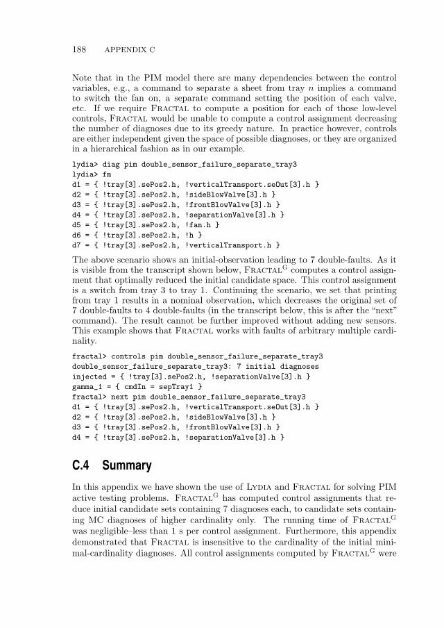
188 APPENDIX C
Note that in the PIM model there are many dependencies between the controlvariables, e.g., a command to separate a sheet from tray n implies a commandto switch the fan on, a separate command setting the position of each valve,etc. If we require Fractal to compute a position for each of those low-levelcontrols, Fractal would be unable to compute a control assignment decreasingthe number of diagnoses due to its greedy nature. In practice however, controlsare either independent given the space of possible diagnoses, or they are organizedin a hierarchical fashion as in our example.
lydia> diag pim double_sensor_failure_separate_tray3
lydia> fm
d1 = !tray[3].sePos2.h, !verticalTransport.seOut[3].h
d2 = !tray[3].sePos2.h, !sideBlowValve[3].h
d3 = !tray[3].sePos2.h, !frontBlowValve[3].h
d4 = !tray[3].sePos2.h, !separationValve[3].h
d5 = !tray[3].sePos2.h, !fan.h
d6 = !tray[3].sePos2.h, !h
d7 = !tray[3].sePos2.h, !verticalTransport.h
The above scenario shows an initial-observation leading to 7 double-faults. As itis visible from the transcript shown below, FractalG computes a control assign-ment that optimally reduced the initial candidate space. This control assignmentis a switch from tray 3 to tray 1. Continuing the scenario, we set that printingfrom tray 1 results in a nominal observation, which decreases the original set of7 double-faults to 4 double-faults (in the transcript below, this is after the “next”command). The result cannot be further improved without adding new sensors.This example shows that Fractal works with faults of arbitrary multiple cardi-nality.
fractal> controls pim double_sensor_failure_separate_tray3
double_sensor_failure_separate_tray3: 7 initial diagnoses
injected = !tray[3].sePos2.h, !separationValve[3].h
gamma_1 = cmdIn = sepTray1
fractal> next pim double_sensor_failure_separate_tray3
d1 = !tray[3].sePos2.h, !verticalTransport.seOut[3].h
d2 = !tray[3].sePos2.h, !sideBlowValve[3].h
d3 = !tray[3].sePos2.h, !frontBlowValve[3].h
d4 = !tray[3].sePos2.h, !separationValve[3].h
C.4 Summary
In this appendix we have shown the use of Lydia and Fractal for solving PIMactive testing problems. FractalG has computed control assignments that re-duce initial candidate sets containing 7 diagnoses each, to candidate sets contain-ing MC diagnoses of higher cardinality only. The running time of FractalG
was negligible–less than 1 s per control assignment. Furthermore, this appendixdemonstrated that Fractal is insensitive to the cardinality of the initial mini-mal-cardinality diagnoses. All control assignments computed by FractalG were

SUMMARY 189
optimal, i.e., no further reduction in the number of initial diagnoses was possible.All this shows that FractalG effectively reduces the diagnostic uncertainty inreal-world models with large number of variables, under-constrained models suchas weak-fault models, or models of sensor-lean systems.

190 APPENDIX C

Bibliography
Ashraf M. Abdelbar. Approximating cost-based abduction is NP-hard. ArtificialIntelligence, 159(1-2):231–239, 2004.
Ashraf M. Abdelbar, Sarah H. Gheita, and Heba A. Amer. Exploring the fitnesslandscape and the run-time behaviour of an iterated local search algorithm forcost-based abduction. Experimental & Theoretical Artificial Intelligence, 18(3):365–386, 2006.
Miron Abramovici. A maximal resolution guided-probe testing algorithm. InProc. DAC’81, pages 189–195, 1981.
Rui Abreu. Spectrum-Based Fault Localization in Embedded Software. PhD thesis,Delft University of Technology, 2009.
Rui Abreu, Peter Zoeteweij, and Arjan van Gemund. A new bayesian approach tomultiple intermittent fault diagnosis. In Proc. IJCAI’09, pages 653–658, 2009.
Rajeev Alur, Costas Courcoubetis, and Mihalis Yannakakis. Distinguishing testsfor nondeterministic and probabilistic machines. In Proc. ACM Symposium onTheory of Computing, pages 363–372, 1995.
Josep Argelich, Chu Min Li, and Felip Manya. An improved exact solver forpartial Max-SAT. In Proc. NCP’07, pages 230–231, 2007.
Mihiar Ayoubi. Fuzzy systems design based on a hybrid neural structure andapplication to the fault diagnosis of technical processes. Control EngineeringPractice, 4(1):35–42, 1996.
James Bailey and Peter J. Stuckey. Discovery of minimal unsatisfiable subsetsof constraints using hitting set dualization. In Proc. PADL’05, pages 174–186,2005.
191
192 BIBLIOGRAPHY
Roberto J. Bayardo and Joseph Daniel Pehoushek. Counting models using con-nected components. In Proc. AAAI’00, pages 157–162, 2000.
Marion Behrens, Gregory Provan, Menouer Boubekeur, and Alie Mady. Model-driven diagnostics generation for industrial automation. In Proc INDIN’09,pages 708–714, 2009.
Franc Brglez and Hideo Fujiwara. A neutral netlist of 10 combinational benchmarkcircuits and a target translator in fortran. In Proc. ISCAS’85, pages 695–698,1985.
Franc Brglez, David Bryan, and Krzysztof Kozminski. Combinational profiles ofsequential benchmark circuits. In Proc. ISCAS’89, volume 3, pages 1929–1934,1989.
Mark Brodie, Irina Rish, Sheng Ma, and Natalia Odintsova. Active probing strate-gies for problem diagnosis in distributed systems. In Proc. IJCAI’03, pages1337–1338, 2003.
Randal E. Bryant. Symbolic Boolean manipulation with ordered binary-decisiondiagrams. ACM Computing Surveys, 24(3):293–318, 1992.
Bruce G. Buchanan and Edward H. Shortliffe, editors. Rule-Based Expert Systems:The MYCIN Experiments of the Stanford Heuristic Programming Project. TheAddison-Wesley Series in Artificial Intelligence. Addison-Wesley, 1984.
Peter Bunus, Olle Isaksson, Beate Frey, and Burkhard Munker. RODON - amodel-based diagnosis approach for the DX diagnostic competition. In Proc.DX’09, pages 423–430, 2009.
Michael L. Bushnell and Vishwani D. Agrawal. Essentials of Electronic Testing forDigital, Memory and Mixed-Signal VLSI Circuits. Kluwer Academic Publishers,Boston, 2000.
Tom Bylander, Dean Allemang, Michael Tanner, and John Josephson. The com-putational complexity of abduction. Artificial Intelligence, 49:25–60, 1991.
Eugene Charniak and Solomon Eyal Shimony. Cost-based abduction and MAPexplanation. Artificial Intelligence, 66(2):345–374, 1994.
SAE Aerospace Propulsion Systems Health Management Committee E-32. Healthand usage monitoring metrics, monitoring the monitor. Technical ReportARP5783, February 2008.
Luca Console and Pietro Torasso. A spectrum of logical definitions of model-baseddiagnosis 1. Computational Intelligence, 7(3):133–141, 1991.
BIBLIOGRAPHY 193
Luca Console, Daniele Theseider Dupre, and Pietro Torasso. On the relationshipbetween abduction and deduction. Journal of Logic Computation, 1(5):661–690,1991.
Luca Console, Claudia Picardi, and Marina Ribaudo. Diagnosis and diagnosabilityanalysis using PEPA. In Proc. ECAI’00, pages 131–135, 2000.
Stephen A. Cook. The complexity of theorem-proving procedures. In Proc.STOC’71, pages 151–158, 1971.
Fulvio Corno, Paolo Prinetto, Maurizio Rebaudengo, and Matteo Sonza Reorda.New static compaction techniques of test sequences for sequential circuits. InProc. EDTC’97, pages 1–37, 1997.
Alexander Czutro, Ilia Polian, Piet Engelke, Sudhakar M. Reddy, and BerndBecker. Dynamic compaction in SAT-based ATPG. In Proc. ATS’09, pages187–190, 2009.
Adnan Darwiche. A differential approach to inference in Bayesian networks. Jour-nal of the ACM, 50(3):280–305, 2003.
Adnan Darwiche. Model-based diagnosis using structured system descriptions.Journal of Artificial Intelligence Research, 8:165–222, 1998.
Adnan Darwiche and Pierre Marquis. A knowlege compilation map. Journal ofArtificial Intelligence Research, 17:229–264, 2002.
Martin Davis and Hilary Putnam. A computing procedure for quantificationtheory. Journal of the ACM, 7(3):201–215, 1960.
Martin Davis, George Logemann, and Donald Loveland. A machine program fortheorem-proving. Communications of the ACM, 5(7):394–397, 1962.
Nando de Freitas. Rao-blackwellised particle filtering for fault diagnosis. In Proc.AEROCONF’02, volume 4, pages 1767–1772, 2002.
Johan de Kleer. An improved approach for generating Max-Fault Min-Cardinalitydiagnoses. In Proc. DX’08, pages 247–252, 2008.
Johan de Kleer. Minimum cardinality candidate generation. In Proc. DX’09,pages 397–402, 2009.
Johan de Kleer. An assumption-based TMS. Artificial Intelligence, 28(2):127–162,1986a.
Johan de Kleer. Problem solving with the ATMS. Artificial Intelligence, 28(2):197–224, 1986b.
194 BIBLIOGRAPHY
Johan de Kleer. Using crude probability estimates to guide diagnosis. ArtificialIntelligence, 45(3):381–291, 1990.
Johan de Kleer and Brian Williams. Diagnosing multiple faults. Artificial Intel-ligence, 32(1):97–130, 1987.
Johan de Kleer, Alan Mackworth, and Raymond Reiter. Characterizing diagnosesand systems. Artificial Intelligence, 56(2-3):197–222, 1992a.
Johan de Kleer, Olivier Raiman, and Mark Shirley. One step lookahead is prettygood. In Readings in Model-Based Diagnosis, pages 138–142. Morgan KaufmannPublishers, San Francisco, 1992b.
Somnath Deb, Sudipto Ghoshal, Venkata N. Malepati, and David L. Kleinman.Tele-diagnosis: Remote monitoring of large-scale systems. In Proc. AERO-CONF’00, volume 6, pages 31–42, 2000.
Richard O. Duda and Edward H. Shortliffe. Expert systems research. Science,220(4594):261–268, 1983.
Charles Ebeling. An Introduction to Reliability and Maintainability Engineering.McGraw-Hill, 1997.
Niklas Een and Niklas Sorensson. An extensible SAT-solver. In Proc. SAT’03,volume 2919 of Lecture Notes in Computer Science, pages 502–518. Springer,2003.
Thomas Eiter and Georg Gottlob. The complexity of logic-based abduction. Jour-nal of the ACM, 42(1):3–42, 1995.
Michael Esser and Peter Struss. Fault-model-based test generation for embeddedsoftware. In Proc. IJCAI’07, 2007.
Alexander Feldman and Arjan van Gemund. A two-step hierarchical algorithmfor model-based diagnosis. In Proc. AAAI’06, 2006.
Alexander Feldman and Arjan van Gemund. Building a Lydia model of an oceprinter’s paper input module. Technical Report TUD-SERG-2007-16, DelftUniversity of Technology, 2007a.
Alexander Feldman and Arjan van Gemund. Lydia user guide. Technical ReportES-2009-05, Delft University of Technology, 2007b.
Alexander Feldman and Arjan van Gemund. Reducing the diagnostic uncertaintyof a paper input module by active testing. Technical Report ES-2009-04, DelftUniversity of Technology, 2009.
Alexander Feldman, Jurryt Pietersma, and Arjan van Gemund. A multi-valuedSAT-based algorithm for faster model-based diagnosis. In Proc. DX’06, 2006.

BIBLIOGRAPHY 195
Alexander Feldman, Gregory Provan, and Arjan van Gemund. Generating mani-festations of max-fault min-cardinality diagnoses. In Proc. DX’07, pages 83–90,2007a.
Alexander Feldman, Gregory Provan, and Arjan van Gemund. Approximatemodel-based diagnosis using greedy stochastic search. In Proc. SARA’07, pages139–154, 2007b.
Alexander Feldman, Gregory Provan, and Arjan van Gemund. A framework andalgorithm for model-based active testing. In Proc. PHM’08, 2008a.
Alexander Feldman, Gregory Provan, and Arjan van Gemund. Computing mini-mal diagnoses by greedy stochastic search. In Proc. AAAI’08, pages 919–924,2008b.
Alexander Feldman, Gregory Provan, and Arjan van Gemund. Computing ob-servation vectors for max-fault min-cardinality diagnoses. In Proc. AAAI’08,pages 911–918, 2008c.
Alexander Feldman, Gregory Provan, Johan de Kleer, Lukas Kuhn, and Arjanvan Gemund. Automated redesign with the General Redesign Engine. In Proc.SARA’09, 2009a.
Alexander Feldman, Gregory Provan, and Arjan van Gemund. FRACTAL: Effi-cient fault isolation using active testing. In Proc. IJCAI’09, 2009b.
Alexander Feldman, Gregory Provan, and Arjan van Gemund. Solving strong-fault diagnostic models by model relaxation. In Proc. IJCAI’09, 2009c.
Alexander Feldman, Tolga Kurtoglu, Sriram Narasimhan, Scott Poll, David Gar-cia, Johan de Kleer, Lukas Kuhn, and Arjan van Gemund. Empirical evaluationof diagnostic algorithm performance using a generic framework. InternationalJournal of Prognostics and Health Management, 2010. Submitted for Review.
Amir Fijany, Farrokh Vatan, Anthony Barrett, Mark James, Colin Williams, andRyan Mackey. A novel model-based diagnosis engine: Theory and applications.In Proc. IEEE Aerospace’03, volume 2, pages 901–910, 2003.
Kenneth Forbus and Johan de Kleer. Building Problem Solvers. MIT Press, 1993.
Lester R. Ford and Delbert R. Fulkerson. Maximal flow through a network.Canadian Journal of Mathematics, 8:399–404, 1956.
Jon W. Freeman. Improvements to Propositional Satisfiability Search Algorithms.PhD thesis, University of Pennsylvania, 1995.
Eugene C. Freuder, Rina Dechter, Matthew L. Ginsberg, Bart Selman, and Ed-ward P. K. Tsang. Systematic versus stochastic constraint satisfaction. In Proc.IJCAI’95, volume 2, pages 2027–2032, 1995.
196 BIBLIOGRAPHY
Gerhard Friedrich, Georg Gottlob, and Wolfgang Nejdl. Physical impossibilityinstead of fault models. In Proc. AAAI’90, pages 331–336, 1990.
Ian P. Gent and Toby Walsh. Towards an understanding of hill-climbing proce-dures for SAT. In Proc. AAAI’93, pages 28–33, 1993.
Ian P. Gent and Toby Walsh. The SAT phase transition. In Proc. ECAI’94, pages105–109, 1994.
Enrico Giunchiglia and Marco Maratea. Solving optimization problems with DLL.In Proc. ECAI’06, pages 377–381, 2006.
Carla P. Gomes, Jorg Hoffmann, Ashish Sabharwal, and Bart Selman. Fromsampling to model counting. In Proc. IJCAI’07, pages 2293–2299, 2007.
Alban Grastien and Priscilla Kan-John. Wizards of oz – description of the 2009DXC entry. In Proc. DX’09, pages 409–413, 2009.
Jun Gu and Ruchir Puri. Asynchronous circuit synthesis with boolean satisfiabil-ity. IEEE Trans. on CAD of Integrated Circuits and Systems, 14(8):961–973,Aug 1995.
Walter Hamscher and Randall Davis. Diagnosing circuits with state: An inher-ently underconstrained problem. In Porc. AAAI’84, pages 142–147, 1984.
Mark Hansen, Hakan Yalcin, and John Hayes. Unveiling the ISCAS-85 bench-marks: A case study in reverse engineering. IEEE Design & Test, 16(3):72–80,1999.
Frederick Hayes-Roth. Rule-based systems. Communications of the ACM, 28(9):921–932, 1985.
David Heckerman, John S. Breese, and Koos Rommelse. Decision-theoretic trou-bleshooting. Communications of the ACM, 38(3):49–57, 1995.
Stefan Heinz and Martin Sachenbacher. Using model counting to find optimaldistinguishing tests. In Proc. of COUNTING’08, pages 91–106, 2008.
Ulrich Heller and Peter Struss. G+DE - the generalized diagnosis engine. In Proc.DX’01, pages 79–86, 2001.
Federico Heras, Javier Larrosa, and Albert Oliveras. MiniMaxSAT: An efficientweighted Max-SAT solver. Journal of Artificial Intelligence Research, 31:1–32,2008.
Miki Hermann and Reinhard Pichler. Counting complexity of propositional ab-duction. In Proc. IJCAI’07, pages 417–422, 2007.
BIBLIOGRAPHY 197
Dorit S. Hochbaum, editor. Approximation Algorithms for NP-hard Problems.PWS Publishing Co., Boston, MA, USA, 1997.
Holger Hoos. SAT-encodings, search space structure, and local search perfor-mance. In Proc. IJCAI’99, pages 296–303, 1999.
Holger Hoos and Thomas Stutzle. Stochastic Local Search: Foundations andApplications. Morgan Kaufmann Publishers Inc., 2004.
Joseph L. A. Hughes. Multiple fault detection using single fault test sets. IEEET-CAD, 7(1):100–108, 1988.
Frank Hutter, Dave A. D. Tompkins, and Holger H. Hoos. Scaling and probabilis-tic smoothing: Efficient dynamic local search for sat. In Proc. CP’02, pages233–248, 2002.
Oscar H. Ibarra and Sartaj K. Sahni. Polynomially complete fault detectionproblems. IEEE Trans. on Computers, 24(3):242–249, 1975.
Rolf Isermann. Supervision, fault-detection and fault-diagnosis methods – anintroduction. Control Engineering Practice, 5(5):639–652, 1997.
HoonSang Jin, HyoJung Han, and Fabio Somenzi. Efficient conflict analysis forfinding all satisfying assignments of a Boolean circuit. In Proc. TACAS’05,pages 287–300, 2005.
L. Karin, R. Lunde, and B. Munker. Model-based failure analysis with RODON.In Proc. ECAI’06, 2006.
Kalev Kask and Rina Dechter. Stochastic local search for Bayesian networks. InProc. AISTAT’99, pages 113–122, 1999.
Alex Kean and George K. Tsiknis. Clause management systems. ComputationalIntelligence, 9:11–40, 1993.
Mark W. Krentel. The complexity of optimization problems. In Proc. STOC’86,pages 69–76, 1986.
Ken Kubiak and W. Kent Fuchs. Multiple-fault simulation and coverage of de-terministic single-fault test sets. In Proc. of the IEEE International Test Con-ference, pages 956–962, 1991.
Lukas Kuhn, Bob Price, Johan de Kleer, Minh Do, and Rong Zhou. Pervasivediagnosis: Integration of active diagnosis into production plans. In Proc. DX’08,pages 106–119, 2008.
T. K. Satish Kumar. A model counting characterization of diagnoses. In Proc.DX’02, pages 70–76, 2002.

198 BIBLIOGRAPHY
O. Erhun Kundakcioglu and Tonguc Unluyurt. Bottom-up construction of mini-mum-cost and/or trees for sequential fault diagnosis. IEEE Trans. on SMC, 37(5):621–629, 2007.
Tolga Kurtoglu, Sriram Narasimhan, Scott Poll, David Garcia, Lukas Kuhn, Jo-han de Kleer, Arjan van Gemund, and Alexander Feldman. First internationaldiagnosis competition - DXC’09. In Proc. DX’09, pages 383–396, 2009.
Jan Eric Larsson. Diagnosis based on explicit means-end models. Artificial Intel-ligence, 80(1), 1996.
Wen-Shing Lee, Doris Grosh, Frank A. Tillman, and Chang H. Lie. Fault treeanalysis, methods, and applications – a review. IEEE Trans. on Reliability,R-34(3):194–202, 1985.
Mark H. Liffiton and Karem A. Sakallah. On finding all minimally unsatisfiablesubformulas. In Proc. SAT’05, pages 173–186, 2005.
Karin Lunde, Rudiger Lunde, and Burkhard Munker. Model-based failure analysiswith RODON. In Proc. ECAI’06, 2006.
Panagiotis Manolios and Daron Vroon. Efficient circuit to CNF conversion. InProc. SAT’07, pages 4–9, 2007.
Joao P. Marques-Silva. The impact of branching heuristics in propositional satis-fiability algorithms. In Proc. EPIA’99, pages 62–74, 1999.
David A. McAllester. Truth maintenance. In Proc. AAAI’90, volume 2, pages1109–1116, 1990.
Ole Mengshoel. Designing resource-bounded reasoners using Bayesian networks:System health monitoring and diagnosis. In Proc. DX’07, pages 330–337, 2007.
Tsoline Mikaelian, Brian C. Williams, and Martin Sachenbacher. Model-basedmonitoring and diagnosis of systems with software-extended behavior. In Proc.AAAI’05, pages 327–333, 2005.
Gordon E. Moore. Cramming more components onto integrated circuits. pages56–59, 2000.
Igor Mozetic and Christian Holzbaur. Controlling the complexity in model-baseddiagnosis. Annals of Mathematics and Artificial Intelligence, 11(1):297–314,1994.
Nicola Muscettola, P. Pandurang Nayak, Barney Pell, and Brian C. Williams.Remote agent: To boldly go where no AI system has gone before. ArtificialIntelligence, 103(1-2):5–47, 1998.
BIBLIOGRAPHY 199
Sriram Narasimhan. Model-Based Diagnosis of Hybrid Systems. PhD thesis,Vanderbilt University, 2002.
Sriram Narasimhan and Lee Brownston. HyDE - a general framework for stochas-tic and hybrid modelbased diagnosis. In Proc. DX’07, pages 162–169, 2007.
Christos H. Papadimitriou. On selecting a satisfying truth assignment. In Proc.FOCS’91, pages 163–169, 1991.
James D. Park. MAP complexity results and approximation methods. In Proc.UAI’02, pages 388–396, 2002.
Krishna Pattipati and Mark Alexandridis. Application of heuristic search andinformation theory to sequential fault diagnosis. IEEE Trans. on SMC, 20(4):872–887, 1990.
Judea Pearl. Probabilistic Reasoning in Intelligent Systems: Networks of PlausibleInference. Morgan Kaufmann, San Francisco, CA, USA, 1988.
Jurryt Pietersma and Arjan van Gemund. Temporal versus spatial observabilityin model-based diagnosis. SMC, 6:5325–5331, 2006.
Jurryt Pietersma and Arjan van Gemund. Benefits and costs of model-based faultdiagnosis for semiconductor manufacturing equipment. In Proc. INCOSE’07,pages 1–12, June 2007.
Scott Poll, Ann Patterson-Hine, Joe Camisa, David Garcia, David Hall, CharlesLee, Ole Mengshoel, Christian Neukom, David Nishikawa, John Ossenfort,Adam Sweet, Serge Yentus, Indranil Roychoudhury, Matthew Daigle, Gau-tam Biswas, and Xenofon Koutsoukos. Advanced diagnostics and prognosticstestbed. In Proc. DX’07, pages 178–185, 2007.
Mukul R. Prasad, Philip Chong, and Kurt Keutzer. Why is ATPG easy. In Proc.DAC’99, pages 22–28, 1999.
Gregory Provan. Test generation for model-based diagnosis. In Proc. ECAI’08,pages 199–203, 2008.
Gregory Provan. Model abstractions for diagnosing hybrid systems. In Proc.DX’09, pages 321–328, 2009.
Gregory Provan and Jun Wang. Automated benchmark model generators formodel-based diagnostic inference. In Proc. IJCAI’07, pages 513–518, 2007.
Vijaya Raghavan, Mojdeh Shakeri, and Krishna Pattipati. Optimal and near-optimal test sequencing algorithms with realistic test models. IEEE Trans. onSMC, 29(1):11–26, 1999.

200 BIBLIOGRAPHY
Anavai Ramesh, George Becker, and Neil Murray. CNF and DNF consideredharmful for computing prime implicants/implicates. Journal of Automated Rea-soning, 18(3):337–356, 1997.
Raymond Reiter. A theory of diagnosis from first principles. Artificial Intelligence,32(1):57–95, 1987.
Dan Roth. On the hardness of approximate reasoning. Artificial Intelligence, 82(1-2):273–302, 1996.
J. Paul Roth. Diagnosis of automata failures: A calculus and a method. IBMJournal of R & D, 10:278–291, 1966.
Indranil Roychoudhury, Gautam Biswas, and Xenofon Koutsoukos. Designingdistributed diagnosers for complex continuous systems. IEEE Trans. on Au-tomation Science and Engineering, 6(2):277–290, 2009.
Meera Sampath, Raja Sengupta, Stephane Lafortune, Kasim Sinnamohideen, andDemosthenis Teneketzis. Diagnosability of discrete event systems. In Proc. onICAOS’94, volume 199, pages 73–79, 1994.
Tian Sang, Paul Beame, and Henry A. Kautz. A dynamic approach for MPE andweighted MAX-SAT. In Proc. IJCAI’07, pages 173–179, 2007.
Eugene Santos Jr. A linear constraint satisfaction approach to cost-based abduc-tion. Artificial Intelligence, 65(1):1–28, 1994.
Marcus Schaefer and Christopher Umans. Completeness in the polynomial-timehierarchy: a compendium. SIGACT News, 2002.
Eugene F. Schuster and William R. Sype. On the negative hypergeometric dis-tribution. International Journal of Mathematical Education in Science andTechnology, 18(3):453–459, 1987.
Bart Selman and Hector J. Levesque. Abductive and default reasoning: a com-putational core. In Proc. AAAI’90, pages 343–348, 1990.
Mojdeh Shakeri. Advances in System Fault Modeling and Diagnosis. PhD thesis,University of Connecticut, 1996.
Mojdeh Shakeri, Vijaya Raghavan, Krishna R. Pattipati, and Ann Patterson-Hine. Sequential testing algorithms for multiple fault diagnosis. IEEE Trans.on SMC, 30(1):1–14, Jan 2000.
Sajjad Siddiqi and Jinbo Huang. Hierarchical diagnosis of multiple faults. InProc. IJCAI’07, pages 581–586, 2007.
Alexander Smith, Andreas Veneris, and Anastasios Viglas. Design diagnosis usingBoolean satisfiability. In Proc. ASP-DAC’04, pages 218–223, 2004.
BIBLIOGRAPHY 201
Alexander Smith, Andreas Veneris, Moayad Fahim Ali, and Anastasios Viglas.Fault diagnosis and logic debugging using Boolean satisfiability. IEEE Trans-actions on CAD of Integrated Circuits and Systems, 24(10):1606–1621, 2005.
Paul Stephan, Robert Brayton, and Alberto Sangiovanni-Vincentelli. Combina-tional test generation using satisfiability. IEEE Trans. on CAD of IntegratedCircuits and Systems, 15(9):1167–1176, 1996.
Peter Struss. Testing physical systems. In Proc. AAAI’94, pages 251–256, 1994.
Peter Struss and Oskar Dressler. Physical negation: Integrating fault models intothe general diagnosis engine. In Proc. IJCAI’89, pages 1318–1323, 1989.
Peter Struss and Oskar Dressler. “Physical negation” - integrating fault modelsinto the General Diagnostic Engine. In Readings in Model-Based Diagnosis,pages 153–158. Morgan Kaufmann Publishers Inc., 1992.
Peter Struss, Andreas Malik, and Martin Sachenbacher. Qualitative modeling isthe key to automated diagnosis. In Proc. IFAC’96, pages 43–48, 1996.
Christian Thiffault, Fahiem Bacchus, and Toby Walsh. Solving non-clausal for-mulas with DPLL search. In Proc. CP’04, pages 663–678, 2004.
Dave A. D. Tompkins and Holger H. Hoos. UBCSAT: An implementation andexperimentation environment for SLS algorithms for SAT and MAX-SAT. InProc. SAT’04, pages 306–320, 2005.
Gregory Tseitin. On the complexity of proofs in propositional logics. In JorgSiekmann and Graham Wrightson, editors, Automation of Reasoning: ClassicalPapers in Computational Logic (1967–1970), volume 2. Springer-Verlag, 1983.
Fang Tu and Krishna Pattipati. Rollout strategies for sequential fault diagnosis.IEEE Trans. on SMC, 33(1):86–99, 2003.
Arjan van Gemund. The Lydia approach to diagnostic systems modeling. Tech-nical Report PDS-2002-004, Delft University of Technology, 2002.
Arjan van Gemund. Lydia version 1.1 tutorial. Technical Report PDS-2003-001,Delft University of Technology, 2003.
John Waicukauski and Eric Lindbloom. Failure diagnosis of structured VLSI.IEEE Design & Test of Computers, 6(4):49–60, Aug 1989.
Brian Williams and Robert Ragno. Conflict-directed A* and its role in model-based embedded systems. Journal of Discrete Applied Mathematics, 155(12):1562–1595, 2007.
Ramin Zabih and David McAllester. A rearrangement search strategy for deter-mining propositional satisfiability. In Proc. AAAI’88, pages 155–160, 1988.

202 BIBLIOGRAPHY
Hantao Zhang and Mark Stickel. Implementing the Davis-Putnam method. JAR,24(1-2):277–296, 2000.
Hantao Zhang and Mark E. Stickel. An efficient algorithm for unit propagation.In Proc. AI-MATH’96, pages 166–169, 1996.
Summary
Approximation Algorithms for Model-Based Diagnosis
Aleksandar Feldman
Model-based diagnosis is an area of abductive inference that uses a system model,together with observations about system behavior, to isolate sets of faulty com-ponents (diagnoses) that explain the observed behavior, according to some mini-mality criterion. This thesis presents greedy approximation algorithms for threeproblems closely related to model-based diagnosis: (1) computation of cardinality-minimal diagnoses, (2) computation of max-fault min-cardinality observation vec-tors, and (3) computation of control assignments that optimally reduce the ex-pected number of remaining cardinality-minimal diagnoses. All three problemsare NP-hard or worse (for example, problem (1) is known to be ΣP
2 -complete forarbitrary propositional models), thus making deterministic algorithms impracticalfor solving large models.
The three main algorithms of this thesis are Safari (StochAstic Fault diag-nosis AlgoRIthm) for problem (1), Miranda (Max-fault mIn-caRdinAlity obser-vatioN Deduction Algorithm) for problem (2), and FractalG (FRamework forACtive Testing ALgorithms - Greedy) for problem (3). These three algorithms,the analysis of their properties, the empirical research about their performance,and the comparison to other approaches are the main theoretical contributions ofthis thesis.
Safari, Miranda, and FractalG employ approximation methods such asgreedy stochastic search, stochastic sampling (in the case of FractalG) and, asa result, efficiently solve worst-case NP -hard or worse problems by trading rela-tively small degradation in the optimality of the diagnostic results for much largergain in the computational performance (in some cases several orders-of-magnitude
203

204 SUMMARY
improvement in speed). This efficient trade-off is partly due to exploitation ofspecific properties in the search landscape of the diagnostic problems. All threealgorithms achieve good optimality at low computational cost in diagnostic searchproblems that exhibit certain amount of continuity.
We have validated the theoretical claims related to Safari, Miranda, andFractalG with extensive experimentation on fault-models of 74XXX/ISCAS85combinational circuits. These models are of variable size (19 – 3 512 compo-nents), different weakness (ignorance of abnormal behaviour, stuck-at), and dif-ferent topology.
We show analytically that for a large class of models (weak-fault models),Safari can be configured to efficiently compute one subset-minimal diagnosis.In the general case (strong-fault model) and in the case of multiple diagnoses weshow topologically-dependent probabilistic properties of Safari. For example, inthe case of multiple diagnoses, Safari computes diagnoses of minimal-cardinalitywith probability which is negative exponential to the cardinality of the minimal-cardinality diagnosis.
Safari is computationally very efficient. For example, Safari computes asubset-minimal diagnosis in a weak-fault model of a digital circuit having morethan 1 500 gates in less than 1 s and the memory footprint is less than 24 Mb ofRAM. The average degradation in the optimality of the diagnoses computed bySafari is 13% only (averaged over all models and observations leading to a singleor double-fault).
We have compared Safari to a range of deterministic and stochastic algo-rithms for computation of cardinality-minimal diagnoses. State-of-the-art deter-ministic algorithms such as HA∗ and CDA∗ are typically several orders-of-mag-nitude slower than Safari. Furthermore HA∗ and CDA∗ often time out withhigher cardinality faults (and larger circuits) whereas Safari is not sensitive tothe cardinality of the cardinality-minimal diagnosis.
Safari has resemblance to Max-SAT and to further empirically analyze theperformance and optimality of Safari, we have implemented a method for com-puting cardinality-minimal diagnoses that uses a deterministic partial Max-SATsolver. In addition to that we have compared Safari to a diagnostic algorithmbased on SLS Max-SAT. We have established that the performance of the com-plete Max-SAT and the optimality of the SLS-based Max-SAT degrade whenincreasing the circuit size or the cardinality of the faults. For example, a diagno-sis algorithm based on W-MaxSatz computed diagnoses with only 9.2% of thec880 observation vectors, whereas Safari always computes at least one nearlyoptimal diagnosis. Algorithms based on SLS-based Max-SAT, typically did notcompute any diagnoses or computed very suboptimal diagnoses (for example oneof the best performing Max-SAT algorithms, SAPS, found a single-fault diagnosisin c7552 after 77 264 restarts, while Safari computed the same diagnosis with 11restarts only).
In this thesis, we propose an algorithm, Miranda, for creating a benchmarkof “difficult” observation vectors for testing the performance and optimality of
SUMMARY 205
diagnostic algorithms such as Safari. Miranda computes observation vectorsleading to faults of high cardinality. These, so-called MFMC observation vectors,lead to diagnoses of cardinality close to the maximally distinguishable given thefault-model. For small combinational circuits (74XXX) the approximations ofMiranda coincide with the optimal MFMC observation vectors (in terms of di-agnostic cardinality) and these results are computed several orders of magnitudefaster than exhaustive algorithms. With large circuits, Miranda computes anMFMC observation vector leading to a diagnosis of approximate cardinality of 36in less than 6 min (c5315). The reason for the good performance of Miranda isthe fact that it exploits continuity in the space of output assignments in a classof well-formed benchmark circuits.
Miranda searches the space of all possible observations, and, at each step,uses Safari to estimate the cardinality of the cardinality-minimal diagnosis. Byvarying the number of Miranda and Safari retries, we have empirically estab-lished lower bounds on the approximation error of Miranda. The theoreticalanalysis of the cardinality estimation optimality of Safari leads us to believethat the small lower bound on the error of Miranda is a good approximationof the overall approximation error and hence, the MFMC values and observationvectors computed by Miranda are nearly optimal.
FractalG is an algorithm that, given a model and an observation leading tomultiple minimal-cardinality diagnoses, computes a control assignment (a test)that optimally reduces the set of diagnoses. As the problem is computationallyhard, we use greedy stochastic search and stochastic sampling. The result is afast algorithm (computing a whole Fractal scenario takes between 1 s for 74182and 15 min for c7552) that decreases the diagnostic uncertainty according to anear-geometric decay curve. The reason for the efficiency of FractalG is thatit exploits continuity in the space of control assignments. Experimentation showsthat this is true even for a small number of control inputs.
FractalG has achieved better exponential decay compared to alternativeapproaches, except exhaustive control search. The difference in the decay ratebetween FractalG and exhaustive search for 74182 is 5.4%. The exhaustivecontrol approach, however, takes minutes to complete even for 74182 and timesout with any model having more than 20 controls.
We have implemented a tool kit for system modeling called Lydia (Languagefor sYstem DIAgnosis). Lydia is also the framework in which we have developedall the algorithms in this thesis. In addition to the implementations of Safari,Miranda, and FractalG, the Lydia tool kit also contains model translators(e.g., to CNF, DNF, OBDDs, etc), utilities, and all reference algorithms.
We have applied Lydia to, amongst others, (1) a model of the Electrical PowerSystem (EPS) testbed in the ADAPT lab at NASA Ames Research Center, as aparticipant in the First International Diagnostic Competition (DXC’09), and (2)a Paper Input Module (PIM), part of a heavy-duty printer of Oce Technologies.The ADAPT EPS consists of electrical components only and the PIM model is acombination of electrical, mechanical and pneumatic ones.

206 SUMMARY
The results from the applications of Lydia to models of physical systems suchas ADAPT and PIM are consistent with the results from experiments on models ofdigital circuits. For example, the average running time of Safari for diagnosingADAPT, a system that is modeled with 723 variables and 1 567 clauses, was below6 s which makes Safari one of the fastest MBD algorithms today.
Samenvatting
Approximation Algorithms for Model-Based Diagnosis
Aleksandar Feldman
Model-gebaseerde diagnose is een vorm van abductie die gebruik maakt van eensysteemmodel en observaties waarme verzamelingen van defecte onderdelen (eendiagnose) worden afgeleid die het waargenomen gedrag verklaren volgens een be-paald minimaliteitscriterium. Dit proefschrift presenteert“greedy”benaderingsal-goritmen voor drie problemen die betrekking hebben op model-gebaseerde diagno-se: (1) berekening van diagnoses van minimale kardinaliteit, (2) berekening vanobservatievectoren overeenkomend met een gemaximaliseerd aantal fouten en eenminimale kardinaliteit, en (3) berekening van de besturingsvector die het verwach-te aantal resterende diagnoses van minimale kardinaliteit minimaliseert. Al dezeproblemen zijn NP -hard of erger (bijvoorbeeld probleem (1) is ΣP
2 -compleet voorwillekeurige propositionele modellen), waardoor het onmogelijk is om determinis-tische algoritmen te gebruiken voor het oplossen van grote modellen.
De drie belangrijkste algoritmen van dit proefschrift zijn Safari (StochAs-tic Fault diagnosis AlgoRIthm) voor Probleem (1), Miranda (Max-fault mIn-caRdinAlity observatioN Deduction Algorithm) voor Probleem (2), en FractalG
(FRamework for ACtive Testing ALgorithms - Greedy) voor Probleem (3). Debelangrijkste theoretische bijdragen van dit proefschrift zijn deze drie algoritmen,de analyse van hun eigenschappen, het empirisch onderzoek naar hun prestaties,en de vergelijking met andere algoritmen.
Safari, Miranda, en FractalG maken gebruik van benaderingsmethodenzoals “greedy stochastic search” en stochastische bemonstering (in het geval vanFractalG). Hiermee kunnen ze worst-case NP -harde of ergere problemen effici-ent oplossen met een relatief kleine afbreuk van de optimaliteit van de diagnosti-
207
208 SAMENVATTING
sche resultaten in te ruilen voor veel grotere winst in de rekenkundige prestaties(in sommige gevallen meerdere orden van grootte verbetering in snelheid). Dezeefficiente uitruil is deels mogelijk door het uitbuiten van specifieke eigenschappenin het zoeklandschap van de diagnostische problemen. Alle drie de algoritmenbereiken een goede optimaliteit tegen lage berekeningskosten in diagnostische op-timaliseringsproblemen die een zekere mate van continuıteit vertonen.
Door middel van uitgebreide experimentering met foutmodellen van 74XXX enISCAS85 combinatorische schakelingen zijn de theoretische claims met betrekkingtot Safari, Miranda en FractalG gevalideerd. Deze modellen hebben varie-rende grootte (19 – 3 512 componenten), verschillende zwakheden (onbekendheidvan abnormaal gedrag, “stuck-at”) en verschillende topologien.
We hebben analytisch aangetoond dat voor een grote klasse van modellen(de zwakke foutmodellen), Safari kan worden geconfigureerd om efficient eenminimale subset diagnose te berekenen. Voor algemene (sterke foutmodellen)en meervoudige diagnosegevallen hebben we topologie-afhankelijke voorspelbareeigenschappen laten zien van Safari. In het geval van meervoudige diagnosesbijvoorbeeld, berekent Safari diagnoses met minimale kardinaliteit met een kansdie negatief exponentioneel is ten opzichte van de kardinaliteit van de diagnosemet minimale kardinaliteit.
Safari is zeer efficient in haar berekeningen. Safari berekent bijvoorbeeldeen minimale subset diagnose in een zwak foutmodel van een digitaal circuit metmeer dan 1 500 poorten in minder dan 1 s met een geheugengebruik van minderdan 24 MB. De gemiddelde optimaliteitsvermindering van de diagnoses berekenddoor Safari is slechts 13% (gemiddeld over alle modellen en observaties die leidentot een enkele - of dubbele fout).
We hebben Safari vergeleken met een aantal deterministische en stochastischealgoritmen voor de berekening van kardinaliteit-minimale diagnoses. Modernedeterministische algoritmen, zoals HA∗ of CDA∗ zijn meestal enkele orden vangrootten minder efficient dan Safari. Bovendien werken HA∗ en CDA∗ vaak nietbij hogere-kardinaliteit fouten (en grotere circuits), terwijl Safari vrijwel nietbeınvloed wordt door de kardinaliteit van de kardinaliteit/minimale diagnose.
Safari is vergelijkbaar met Max-SAT. Om de prestaties en optimaliteit vanSafari empirisch te analyseren, hebben we een methode geınplementeerd voorhet berekenen van kardinaliteit-minimal diagnoses dat gebruik maakt van deter-ministische partiele Max-SAT solver. Daarnaast hebben we Safari vergelekenmet een diagnostisch algoritme gebaseerd op SLS Max-SAT. We hebben vast-gesteld dat de prestaties van de complete Max-SAT en de optimaliteit van deSLS-gebaseerde Max-SAT verminderen wanneer de circuit grootte of de kardina-liteit van de fouten stijgen. Een algoritme gebaseerd op W-MaxSatz berekentbijvoorbeeld diagnoses met slechts 9.2 % van de c880 observatievectoren, terwijlSafari altijd ten minste een bijna optimale diagnose berekent. SLS-gebaseerdealgoritmen voor Max-SAT berekenen meestal geen diagnoses of berekenen zeersuboptimale diagnoses (een van de best presterende Max-SAT algoritmen, SAPS,vond bijvoorbeeld een enkele-fault diagnose in c7552 na 77 264 herstarts, terwijl
SAMENVATTING 209
Safari dezelfde diagnose berekent met slechts 11 herstarts.In dit proefschrift stellen we een algoritme genaamd Miranda voor, voor de
berekening van een benchmark van “moeilijk” observatievectoren voor het testenvan de prestaties en optimaliteit van diagnostische algoritmen, zoals Safari. Mi-
randa berekent observatievectoren die leiden tot fouten van hoge kardinaliteit.Deze zogenaamde MFMC observatievectoren leiden tot diagnoses van kardinali-teit dicht bij die van het gegeven foutmodel. Voor kleine combinatorische circuits(74XXX) vallen de benaderingen van Miranda samen met de optimale MFMCwaarnemingsvectoren (in termen van diagnostische kardinaliteit) en worden dezeresultaten diverse orden van grootte sneller berekend dan uitputtende algoritmen.Voor grote circuits berekent Miranda een MFMC observatievector die leidt toteen diagnose met kardinaliteit van ongeveer 36 in minder dan 6 min (c5315). Dereden van de goede prestaties van Miranda is het feit dat zij de continuıteit in deruimte van de output opdrachten uitbuit die bestaat in de klasse van welgevormdebenchmarkcircuits.
Miranda doorzoekt de ruimte van alle mogelijke observaties, en gebruikt bijelke stap Safari voor de berekening van de kardinaliteit van de diagnose met mi-nimale kardinaliteit. Door het aantal Miranda en Safari pogingen te varieren,hebben we empirisch ondergrenzen van de approximatiefout van Miranda vast-gesteld. De theoretische analyse van de optimaliteit van de kardinaliteitsschattingvan Safari geeft ons vertrouwen dat de kleine ondergrens van de fout van Miran-
da een goede benadering is van de globale benaderingsfout, en daarmee dat dedoor Miranda berekende MFMC waarden en observatievectoren bijna optimaalzijn.
FractalG is een algoritme dat, gegeven een model en een observatie die leidentot een verzameling van meerdere diagnoses met minimale kardinaliteit, een be-sturingsvector (test) berekent die die verzameling optimaal reduceert. Aangezienhet probleem berekeningstechnisch moeilijk is, gebruiken we een“greedy”stochas-tisch zoekalgoritme samen met een stochastische bemonstering. Het resultaat iseen snel algoritme (een geheel Fractal scenario neemt tussen 1 s voor 74182en 15 min voor c7552) dat de diagnostische onzekerheid vermindert volgens eenbijna-geometrische afname-curve. De reden voor de efficientie van FractalG isdat het de continuıteit in de ruimte van besturingsvectoren uitbuit. Experimententonen aan dat dit zelfs waar is voor een klein aantal besturingsvariabelen.
FractalG bereikt een betere exponentiele afname dan alternatieve algorit-men, met uitzondering van “exhaustive search”. Het verschil in afnamesnelheidtussen FractalG en exhaustive search voor 74182 is 5.4 %. Daarentegen heeftexhaustive search minuten nodig voor 74182 (het kleinste model) en bereikt hetde tijdslimiet voor ieder model met meer dan 20 besturingsvariabelen.
We hebben een toolkit voor systeemmodellering geımplementeerd, genaamdLydia (Language for sYstem DIAgnosis). Lydia is ook het raamwerk waarbinnenalle algorithmen in deze thesis zijn ontwikkeld. Naast implementaties van Safari,Miranda, en FractalG, bevat de Lydia toolkit ook modelvertalers (bv. naarCNF, DNF, OBDDs etc.), utilities, and alle referentie-algorithmen.

210 SAMENVATTING
We hebben Lydia onder meer toegepast op (1) een model van het ElectricalPower System (EPS) testbed van het ADAPT laboratorium van NASA Ames Re-search Center, als deelnemer aan de First International Diagnostic Competition(DXC’09), en (2) een Paper Input Module (PIM), onderdeel van een industrieleprinter van Oce Technologies. Het ADAPT EPS bestaat uit enkele electrischecomponenten, terwijl het PIM model een combinatie is van electrische, mechani-sche, en pneumatische componenten.
De resulaten van de toepassing van Lydia op modellen van fysieke systemenzoals ADAPT en PIM komen overeen met die van experimenten met modellen vandigitale circuits. Bijvoorbeeld, de gemiddelde executietijd van Safari voor hetdiagnostiseren van ADAPT, een systeem dat is gemodelleerd met 723 variabelenen 1 567 clauses, blijft onder de 6 s, hetgeen Safari vandaag-de-dag tot een vande snelste MBD algoritmen maakt.

Curriculum Vitae
Personal Data
Date of Birth: September 17, 1977
Address: Willem van Aelststraat 9/22612 HR DelftThe Netherlands
Tel.: +31 15 2129502
Cellular: +31 612 973650
email: [email protected]
URL: http://llama.gs/
Education
9/2005–5/2010 Ph.D., Computer ScienceDelft University of Technology, The Netherlands
Thesis: Approximation Algorithms for Model-Based DiagnosisAdvisor: Prof. Arjan van Gemund
9/2002–9/2004 M.Sc. (cum laude), Computer Science (Technical Informatics)Delft University of Technology, The Netherlands
Thesis: Hierarchical Approach to Fault DiagnosisAdvisor: Prof. Arjan van Gemund
9/1997–6/2000 B.Sc., Computer ScienceUE Varna, Bulgaria
211

212 CURRICULUM VITAE
Employment
5/2008–9/2008 Visiting ResearcherIntelligent Systems Laboratory, Embedded Reasoning AreaPalo Alto Research Center (PARC), Inc.California, USA
9/2005–5/2010 Doctoral Research FellowFaculty of Electrical Engineering, Mathematics andComputer Science, Delft University of TechnologyThe Netherlands
4/2005–9/2005 Software ArchitectScience and Technology BV, Delft, The Netherlands
9/2001–4/2005 Senior ProgrammerMarket Risk Management, ING Bank, AmsterdamThe Netherlands
7/2000–9/2001 Senior ProgrammerZend Technologies Ltd., Ramat Gan, Israel
Professional Activities
Reviewer Journal on Artificial Intelligence (AIJ)Journal of Universal Computer Science (JUCS)Journal on Systems, Man and Cybernetics (SMC)IEEE Transactions on Reliability (TREL)International Workshop on Principles of Diagnosis 2010 (DX’10)International Workshop on Principles of Diagnosis 2009 (DX’09)International Conference on Prognostics and Health Management2008 (PHM’08)
Organizer Second International Diagnostic Competition (DXC’10)First International Diagnostic Competition (DXC’09)
Teaching Experience
9/2007–1/2008 Model-Based Computing, Delft University of TechnologyTeaching assistant
2/2007–3/2007 Model-Checking, Delft University of TechnologyTeaching assistant
Scholarship and Prizes
M.Sc. cum laude
Best paper award at the First International Conference on Prog-nostics and Health Management 2008 (PHM’08)
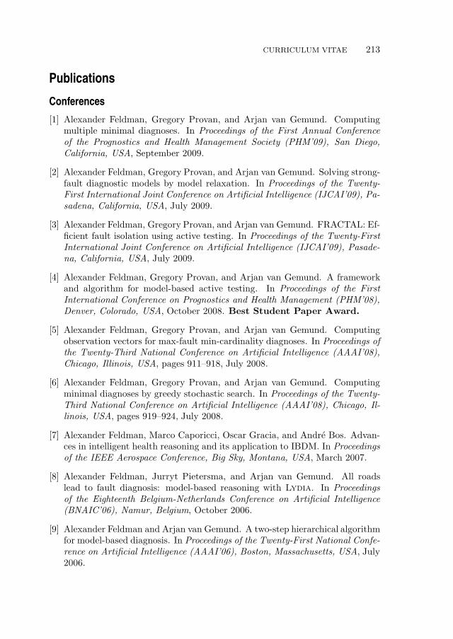
CURRICULUM VITAE 213
Publications
Conferences
[1] Alexander Feldman, Gregory Provan, and Arjan van Gemund. Computingmultiple minimal diagnoses. In Proceedings of the First Annual Conferenceof the Prognostics and Health Management Society (PHM’09), San Diego,California, USA, September 2009.
[2] Alexander Feldman, Gregory Provan, and Arjan van Gemund. Solving strong-fault diagnostic models by model relaxation. In Proceedings of the Twenty-First International Joint Conference on Artificial Intelligence (IJCAI’09), Pa-sadena, California, USA, July 2009.
[3] Alexander Feldman, Gregory Provan, and Arjan van Gemund. FRACTAL: Ef-ficient fault isolation using active testing. In Proceedings of the Twenty-FirstInternational Joint Conference on Artificial Intelligence (IJCAI’09), Pasade-na, California, USA, July 2009.
[4] Alexander Feldman, Gregory Provan, and Arjan van Gemund. A frameworkand algorithm for model-based active testing. In Proceedings of the FirstInternational Conference on Prognostics and Health Management (PHM’08),Denver, Colorado, USA, October 2008. Best Student Paper Award.
[5] Alexander Feldman, Gregory Provan, and Arjan van Gemund. Computingobservation vectors for max-fault min-cardinality diagnoses. In Proceedings ofthe Twenty-Third National Conference on Artificial Intelligence (AAAI’08),Chicago, Illinois, USA, pages 911–918, July 2008.
[6] Alexander Feldman, Gregory Provan, and Arjan van Gemund. Computingminimal diagnoses by greedy stochastic search. In Proceedings of the Twenty-Third National Conference on Artificial Intelligence (AAAI’08), Chicago, Il-linois, USA, pages 919–924, July 2008.
[7] Alexander Feldman, Marco Caporicci, Oscar Gracia, and Andre Bos. Advan-ces in intelligent health reasoning and its application to IBDM. In Proceedingsof the IEEE Aerospace Conference, Big Sky, Montana, USA, March 2007.
[8] Alexander Feldman, Jurryt Pietersma, and Arjan van Gemund. All roadslead to fault diagnosis: model-based reasoning with Lydia. In Proceedingsof the Eighteenth Belgium-Netherlands Conference on Artificial Intelligence(BNAIC’06), Namur, Belgium, October 2006.
[9] Alexander Feldman and Arjan van Gemund. A two-step hierarchical algorithmfor model-based diagnosis. In Proceedings of the Twenty-First National Confe-rence on Artificial Intelligence (AAAI’06), Boston, Massachusetts, USA, July2006.
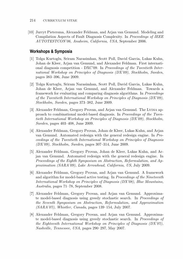
214 CURRICULUM VITAE
[10] Jurryt Pietersma, Alexander Feldman, and Arjan van Gemund. Modeling andCompilation Aspects of Fault Diagnosis Complexity. In Proceedings of IEEEAUTOTESTCON’06, Anaheim, California, USA, September 2006.
Workshops & Symposia
[1] Tolga Kurtoglu, Sriram Narasimhan, Scott Poll, David Garcia, Lukas Kuhn,Johan de Kleer, Arjan van Gemund, and Alexander Feldman. First internati-onal diagnosis competition - DXC’09. In Proceedings of the Twentieth Inter-national Workshop on Principles of Diagnosis (DX’09), Stockholm, Sweden,pages 383–396, June 2009.
[2] Tolga Kurtoglu, Sriram Narasimhan, Scott Poll, David Garcia, Lukas Kuhn,Johan de Kleer, Arjan van Gemund, and Alexander Feldman. Towards aframework for evaluating and comparing diagnosis algorithms. In Proceedingsof the Twentieth International Workshop on Principles of Diagnosis (DX’09),Stockholm, Sweden, pages 373–382, June 2009.
[3] Alexander Feldman, Gregory Provan, and Arjan van Gemund. The Lydia ap-proach to combinational model-based diagnosis. In Proceedings of the Twen-tieth International Workshop on Principles of Diagnosis (DX’09), Stockholm,Sweden, pages 403–408, June 2009.
[4] Alexander Feldman, Gregory Provan, Johan de Kleer, Lukas Kuhn, and Arjanvan Gemund. Automated redesign with the general redesign engine. In Pro-ceedings of the Twentieth International Workshop on Principles of Diagnosis(DX’09), Stockholm, Sweden, pages 307–314, June 2009.
[5] Alexander Feldman, Gregory Provan, Johan de Kleer, Lukas Kuhn, and Ar-jan van Gemund. Automated redesign with the general redesign engine. InProceedings of the Eighth Symposium on Abstraction, Reformulation, and Ap-proximation (SARA’09), Lake Arrowhead, California, US, July 2009.
[6] Alexander Feldman, Gregory Provan, and Arjan van Gemund. A frameworkand algorithm for model-based active testing. In Proceedings of the NineteenthInternational Workshop on Principles of Diagnosis (DX’08), Blue Mountains,Australia, pages 71–78, September 2008.
[7] Alexander Feldman, Gregory Provan, and Arjan van Gemund. Approxima-te model-based diagnosis using greedy stochastic search. In Proceedings ofthe Seventh Symposium on Abstraction, Reformulation, and Approximation(SARA’07), Whistler, Canada, pages 139–154, July 2007.
[8] Alexander Feldman, Gregory Provan, and Arjan van Gemund. Approxima-te model-based diagnosis using greedy stochastic search. In Proceedings ofthe Eighteenth International Workshop on Principles of Diagnosis (DX’07),Nashville, Tennessee, USA, pages 290–297, May 2007.
CURRICULUM VITAE 215
[9] Alexander Feldman, Gregory Provan, and Arjan van Gemund. Generatingmanifestations of max-fault min-cardinality diagnoses. In Proceedings of theEighteenth International Workshop on Principles of Diagnosis (DX’07), Na-shville, Tennessee, USA, pages 83–90, May 2007.
[10] Alexander Feldman, Gregory Provan, and Arjan van Gemund. Interchangeformats and automated benchmark model generators for model-based dia-gnostic inference. In Proceedings of the Eighteenth International Workshopon Principles of Diagnosis (DX’07), Nashville, Tennessee, USA, pages 91–98,May 2007.
[11] Alexander Feldman, Jurryt Pietersma, and Arjan van Gemund. A multi-valued SAT-based algorithm for faster model-based diagnosis. In Proceedingsof the Seventeenth International Workshop on Principles of Diagnosis (DX’06),Penaranda de Duero, Burgos, Spain, June 2006.
[12] Alexander Feldman, Arjan van Gemund, and Andre Bos. A hybrid approachto hierarchical fault diagnosis. In Proceedings of the Sixteenth InternationalWorkshop on Principles of Diagnosis (DX’05), Monterey, California, USA,pages 101–106, June 2005.
Technical Reports
[1] Alexander Feldman, Gregory Provan, and Arjan van Gemund. A family ofmodel-based diagnosis algorithms based on Max-SAT. Technical Report ES-2009-02, Delft University of Technology, 2009.
[2] Alexander Feldman and Arjan van Gemund. Reducing the diagnostic uncer-tainty of a paper input module by active testing. Technical Report ES-2009-04,Delft University of Technology, 2009.
[3] Alexander Feldman and Arjan van Gemund. Lydia user guide. TechnicalReport ES-2009-05, Delft University of Technology, 2007.
[4] Alexander Feldman and Arjan van Gemund. Building a Lydia Model of anOce Printer’s paper input module. Technical Report TUD-SERG-2007-16,Delft University of Technology, 2007.
Journal Papers in Review
[1] Alexander Feldman, Gregory Provan, and Arjan van Gemund. Approximatemodel-based diagnosis using greedy stochastic search. Journal of ArtificialIntelligence Research, 2010. Submitted for Review.
[2] Alexander Feldman, Gregory Provan, and Arjan van Gemund. Stochasticalgorithms for sequential model-based diagnosis. Journal of Artificial Intelli-gence Research, 2010. Submitted for Review.

216 CURRICULUM VITAE
[3] Alexander Feldman, Tolga Kurtoglu, Sriram Narasimhan, Scott Poll, DavidGarcia, Johan de Kleer, Lukas Kuhn, and Arjan van Gemund. EmpiricalEvaluation of Diagnostic Algorithm Performance Using a Generic Framework.International Journal of Prognostics and Health Management, 2010. Submit-ted for Review.


2502367890909
ISBN 978-90-9025023-6
90000 >