Efficient Approximation Algorithms for SchedulingMoldable TasksXIAOHU WU, Nanyang Technological University, SingaporePATRICK LOISEAU, Univ. Grenoble Alpes, Inria, CNRS, Grenoble INP, LIG, France

We study the problem of scheduling 𝑛 independent moldable tasks on 𝑚 processors that arises in large-scaleparallel computations. When tasks are monotonic, the best known result is a ( 32 + 𝜖)-approximation algorithmfor makespan minimization with a complexity linear in 𝑛 and polynomial in log𝑚 and 1

𝜖 where 𝜖 is arbitrarilysmall. We propose a new perspective of the existing speedup models: the speedup of a task 𝑇𝑗 is linear whenthe number 𝑝 of assigned processors is small (up to a threshold 𝛿 𝑗 ) while it presents monotonicity when 𝑝

ranges in [𝛿 𝑗 , 𝑘 𝑗 ]; the bound 𝑘 𝑗 indicates an unacceptable overhead when parallelizing on too many processors.

For a given integer 𝛿 ≥ 5, let 𝑢 =

⌈2√𝛿

⌉− 1. In this paper, we propose a 1

\ (𝛿) (1 + 𝜖)-approximation algorithm

for makespan minimization with a complexity O(𝑛 log(𝑛/𝜖) log𝑚) where \ (𝛿) = 𝑢+1𝑢+2

(1 − 𝑘

𝑚

)(𝑚 ≫ 𝑘). As

a by-product, we also propose a \ (𝛿)-approximation algorithm for throughput maximization with a commondeadline with a complexity O(𝑛2 log𝑚).

Additional Key Words and Phrases: Scheduling, approximation algorithms, moldable tasks

1 INTRODUCTIONMost computations nowadays are done in a parallelized way on large computers containing many

processors. Optimizing the use of processors leads to the problem of scheduling parallel tasks basedon their characteristics. In certain cases, the number of processors assigned to a task is predefinedby its owner and is said to be rigid. However, in many cases, the scheduler can decide this numberbefore the task execution: if this number cannot be changed during the task execution, the task issaid to be moldable; otherwise, it is said to be malleable1. Moldable tasks are easier to implementand manage than malleable tasks; the latter require additional system support for task migrations andpreemptions [7].

1.1 General Problem DescriptionWe consider the problem of scheduling 𝑛 independent moldable tasks T = {𝑇1,𝑇2, · · · , 𝑇𝑛} on

𝑚 identical processors; all tasks are available at time zero. For every task 𝑇𝑗 ∈ T , its executiontime 𝑡 𝑗,1 on one processor is given, as well as the speedup [ 𝑗,𝑝 when assigned 𝑝 > 1 processors;the execution time of 𝑇𝑗 on 𝑝 processors is 𝑡 𝑗,𝑝 =

𝑡 𝑗,1[ 𝑗,𝑝

and its workload is 𝐷 𝑗,𝑝 = 𝑡 𝑗,𝑝𝑝. 𝑇𝑗 can berepresented by a rectangle in the processors × time space. Like [14, 22, 23], given a real number 𝑑 ,we define a parameter 𝛾 ( 𝑗, 𝑑) as the minimum number of processors needed to finish task 𝑇𝑗 by time𝑑; by convention, we set 𝛾 ( 𝑗, 𝑑) = +∞ to imply the case that 𝑇𝑗 cannot be finished by time 𝑑 on anynumber of processors.

We often hope to finish all tasks as soon as possible. Sometimes, a task 𝑇𝑗 also has a value 𝑣 𝑗 thatcan be obtained if it is finished by a deadline 𝜏 ; then we hope to finish by time 𝜏 the most valuabletasks. We will propose algorithms that generate schedules for different objectives: (i) minimize themakespan, i.e., the maximum completion time of all tasks of T or (ii) choose a subset of tasks andfinish them on the 𝑚 processors by a deadline 𝜏 to maximize the throughput, i.e., the aggregate

1In the earlier literature, moldable tasks was also called malleable tasks. Now, malleable tasks refer to another type of paralleltasks [7].

Authors’ addresses: Xiaohu Wu, Nanyang Technological University, Singapore, xiaohu.wu@ntu.edu.sg; Patrick Loiseau,Univ. Grenoble Alpes, Inria, CNRS, Grenoble INP, LIG, France, patrick.loiseau@inria.fr.

arX

iv:1

609.

0858

8v11

[cs

.DS]

20

Nov

202

1

2 Wu and Loiseau

value of tasks finished by time 𝜏 . For each task to be executed, a schedule will define the numberof processors assigned to it and the time interval in which it is finished. For our minimization (resp.maximization) problem, an algorithm is a 𝜌-approximation if it produces a schedule whose makespanis at most 𝜌 times the optimal makespan where 𝜌 ≥ 1 (resp. whose throughput is at least 𝜌 times theoptimal throughput where 𝜌 ≤ 1). It is always desired to have performance bound 𝜌 closer to one,while keeping algorithms simple to run efficiently.

1.2 Typical Speedup Models, and MotivationFor moldable tasks, a key aspect that conditions scheduling is the relation between the task

execution time and the number of assigned processors. Now, we introduce several typical speedupmodels in literature and the most related works under each model, as well as the main motivation fordeveloping the ideas of this paper. Like ours, these works consider offline scheduling of independentmoldable tasks for makespan minimization, except [6, 10, 12, 26, 28].Linear-Speedup Model. An ideal speedup model is linear, i.e., [ 𝑗,𝑝 = 𝑝, when 𝑝 does not exceeda threshold 𝛿 𝑗 [7]; the workload of 𝑇 𝑗 is independent of 𝑝 since 𝐷 𝑗,𝑝 =

𝑡 𝑗,1[ 𝑗,𝑝

𝑝 = 𝑡 𝑗,1. This modelapplies to embarrassingly parallel tasks [4, 29]: each task consists of many independent subtasksthat can simultaneously be executed on multiple processors without any communication overhead.Benoit et al. propose a list-based scheduling algorithm, called LPA-LIST, for failure-prone platformswith additional constraints and show that it is a 2-approximation [3]. When there are precedenceconstraints among moldable tasks, Wang et al. propose a

(3 − 2

𝑚

)-approximation algorithm [26].

Besides, the case of scheduling independent malleable tasks has well been studied [6, 12, 28].Communication Models. When communication is needed among the subtasks of a task 𝑇𝑗 , it istypical of parallel applications that the speedup is still linear when 𝑝 is within a relatively small 𝛿 𝑗 ;afterwards, the speedup is sublinear (i.e., [ 𝑗,𝑝 < 𝑝) and assigning more than 𝛿 𝑗 processors to execute𝑇𝑗 becomes less efficient due to the communication overheads [6]. Such tasks can be simplifiedand still treated as tasks with linear speedup by limiting that the maximum number of processorsassigned to𝑇𝑗 is 𝛿 𝑗 , although it may be worth exploring the opportunity of assigning more processorsto get better resource efficiency. Another typical speedup function is as follows: 𝑡 𝑗,𝑝 =

𝑡 𝑗,1𝑝+ (𝑝 − 1)𝑐 𝑗 ;

the term (𝑝 − 1)𝑐 𝑗 implies that, as more processors are assigned, the overhead and workload 𝐷 𝑗,𝑝

increase; if 𝑝 is too large, 𝑡 𝑗,𝑝 will not decrease as 𝑝 increases. Then, Havill et al. propose an onlinealgorithm with an approximation ratio 4(𝑚−1)

𝑚for even 𝑚 ≥ 2 and 4𝑚

𝑚+1 for odd 𝑚 ≥ 3 [10]; Benoit etal. also show that LPA-LIST is a 3-approximation for failure-prone platforms [3]. As elaborated later,these speedup modes are also validated empirically and consistent.Monotonic Model. To date, the best algorithms for our problem are designed by simply using ageneral monotonic assumption: the execution time of 𝑇𝑗 is non-increasing and its workload is non-decreasing in 𝑝, where [ 𝑗,𝑝 ≤ 𝑝. Belkhale et al. give a 2

1+1/𝑚 -approximation algorithm [2]. Mounié

et al. propose a (√3+ 𝜖)-approximation algorithm and then a ( 32 + 𝜖)-approximation algorithm with

a complexity O(𝑚𝑛 log 𝑛𝜖) where 𝜖 is arbitrarily small [22, 23]. Jansen et al. achieve an improved

complexity polynomial in log𝑚 and 1𝜖

and linear in 𝑛, although their algorithm is still a ( 32 + 𝜖)-approximation [14]. In the special case where 𝑚 ≥ 8𝑛

𝜖, they also give a fully polynomial time

approximation scheme (FPTAS) with a complexity O(𝑛 log2𝑚(log𝑚 + log 1𝜖)). The FPTAS requires

a specific relation between 𝑛 and𝑚.In the case where 𝑛 is independent of𝑚, we hope to develop a 𝜌-approximation algorithm with

𝜌 < 32 and will revisit the related speedup models. Under the monotonic assumption, we have the

following bounds of the execution time 𝑡 𝑗,𝛾 ( 𝑗,𝑑) when a task 𝑇𝑗 is assigned 𝛾 ( 𝑗, 𝑑) processors, which

Efficient Approximation Algorithms for Scheduling Moldable Tasks 3

will also hold in this paper:

𝑑 ≥ 𝑡 𝑗,𝛾 ( 𝑗,𝑑) >𝛾 ( 𝑗, 𝑑) − 1𝛾 ( 𝑗, 𝑑) 𝑑. (1)

By the definition of 𝛾 ( 𝑗, 𝑑), 𝐷 𝑗,𝛾 ( 𝑗,𝑑) is the minimum workload needed to complete 𝑇𝑗 by time𝑑. Suppose that an algorithm produces a schedule of a makespan 𝑑. We observe that it is a 1

\-

approximation to makespan minimization if every task 𝑇𝑗 ∈ T has the minimum workload and theaggregate workload processed on the𝑚 processors in [0, 𝑑] is ≥ \𝑚𝑑 where \ is a lower bound ofthe processor utilization. Our objective is to make \ large (e.g., \ > 2

3 ). For each task 𝑇𝑗 with large𝛾 ( 𝑗, 𝑑) (e.g., 𝛾 ( 𝑗, 𝑑) ≥ 4), we have by Inequality (1) that executing it on 𝛾 ( 𝑗, 𝑑) processors alone canmake these processors achieve a high utilization in [0, 𝑑]. One main challenge comes from tasks withsmaller 𝛾 ( 𝑗, 𝑑). Then, a more precise speedup description than monotonicity could help, which isfortunately available in literature; it allows quantitatively characterizing the execution time reductionwhile keeping the workload constant, when the number of processors assigned to 𝑇𝑗 changes from𝛾 ( 𝑗, 𝑑) to a larger value. We can thus obtain some desired properties and design a schedule underwhich the 𝑚 processors achieve a high overall utilization in [0, 𝑑] under some additional constraints(see Section 3).

In fact, the speedup function in the communication model above is validated on widely used NASparallel benchmarks and HPLinpack, which contain multiple computations with typical communi-cation patterns for evaluating the performance of parallel systems [18]. The benchmarking resultsof [8] indicate that 𝑐 𝑗 is far smaller than 𝑡 𝑗,1 such that when 𝑝 is small, the effect of (𝑝 − 1)𝑐 𝑗 on𝑡 𝑗,𝑝 is negligible compared with the term 𝑡 𝑗,1

𝑝, and the speedup coincides quite accurately with the

linear-speedup model. Thus, we associate such a task 𝑇𝑗 with two thresholds 𝛿 𝑗 and 𝑘 𝑗 to distinguishthe speedup modes of 𝑇𝑗 when 𝑝 is in different ranges where 𝛿 𝑗 ≤ 𝑘 𝑗 ; then, we make the followingdefinition on which we will base the algorithmic design of this paper.

DEFINITION 1. A task 𝑇𝑗 ∈ T is said to be (𝛿 𝑗 , 𝑘 𝑗 )-monotonic if it is moldable and satisfies(1) when 𝑝 ∈ [1, 𝛿 𝑗 ], its workload remains constant and the speedup is linear, i.e., 𝐷 𝑗,1 = 𝐷 𝑗,𝑝 =

𝑡 𝑗,𝑝𝑝;(2) If 𝛿 𝑗 < 𝑘 𝑗 , its workload is increasing while its execution time is decreasing in 𝑝 ∈ [𝛿 𝑗 , 𝑘 𝑗 ], i.e.,

𝐷 𝑗,𝑝 < 𝐷 𝑗,𝑝+1 and 𝑡 𝑗,𝑝 > 𝑡 𝑗,𝑝+1 for 𝑝 ∈ [𝛿 𝑗 , 𝑘 𝑗 − 1].(3) The parameter 𝑘 𝑗 is a parallelism bound, i.e., the maximum number of processors allowed to

be assigned to 𝑇𝑗 .

Particularly, if 𝑘 𝑗 = 𝛿 𝑗 , then a (𝛿 𝑗 , 𝑘 𝑗 )-monotonic task is simply a task whose speedup is linearwithin a parallelism bound 𝛿 𝑗 . In Definition 1, the second point implies that assigning more than 𝛿 𝑗for executing 𝑇𝑗 is less efficient but its execution time is decreasing in 𝑝 ∈ [𝛿 𝑗 , 𝑘 𝑗 ]. The third point isused to reflect that when 𝑝 > 𝑘 𝑗 , the workload begins to increase to an unacceptable extent such thatthe execution time does not decrease any more (i.e., [ 𝑗,𝑘 𝑗

≥ [ 𝑗,𝑝 ), which implies that assigning morethan 𝑘 𝑗 processors to 𝑇𝑗 cannot bring any benefit. The parameters 𝛿 𝑗 and 𝑘 𝑗 are fixed; as reported in[8], 𝛿 𝑗 and 𝑘 𝑗 can range in [25, 150] and [250, 512], depending on the types of computation embodiedin the tasks of T . The number𝑚 of processors is large since our problem arises in large-scale parallelsystems, e.g., supercomputers can have𝑚 = 216 processors inside [1, 27].

1.3 Algorithmic ResultsConsider a set T in which each task 𝑇𝑗 is (𝛿 𝑗 , 𝑘 𝑗 )-monotonic. We denote by 𝛿 the minimum

linear-speedup threshold of all tasks of T and by 𝑘 the maximum parallelism bound of all tasks of T ,i.e.,

𝛿 = min𝑇𝑗 ∈T{𝛿 𝑗 } and 𝑘 = max𝑇𝑗 ∈T{𝑘 𝑗 }. (2)

4 Wu and Loiseau

Let 𝑢 =

⌈2√𝛿

⌉− 1, that is, 𝑢 is the unique integer such that 𝛿 ∈ [𝑢2 + 1, (𝑢 + 1)2]. In this paper,

for any 𝛿 ≥ 5, the main algorithmic result is a 1\ (𝛿) (1 + 𝜖)-approximation algorithm for makespan

minimization with a complexity O(𝑛 log(𝑛/𝜖) log𝑚) where

\ (𝛿) = 𝑢 + 1𝑢 + 2

(1 − 𝑘

𝑚

).

The algorithm achieves an approximation ratio \ (𝛿) close to 𝑢+2𝑢+1 since 𝑚 ≫ 𝑘. Typically, the

minimum linear-speedup threshold 𝛿 has an effective range of [25, 150] [8]. In the worst case that𝛿 = 25, \ (𝛿) is close to 6

5 ; when 𝛿 = 150, 𝑢+2𝑢+1 = 14

13 ≈ 1.077, which is close to 1. The larger thelinear-speedup threshold 𝛿 , the better the proposed algorithm. For throughput maximization with agiven deadline 𝜏 , we assume that every task 𝑇𝑗 ∈ T can be finished by time 𝜏 , i.e., 𝛾 ( 𝑗, 𝑑) ∈ [1,𝑚].As a by-product, another algorithmic result of this paper is a \ (𝛿)-approximation algorithm with acomplexity O(𝑛2 log𝑚) to maximize the throughput with a deadline 𝜏 . To the best of our knowledge,we are the first to address this scheduling objective for moldable tasks, while this objective has beenaddressed for other types of parallel tasks in the literature of scheduling theory [9, 17].

The rest of this paper is organized as follows. In Section 2, we give more related work. In Section 3,we give an overview of the ideas developed in this paper. The following two sections are used toelaborate these ideas. In particular, in Section 4, we propose an algorithm that produces a schedulewith several features described in Section 3. In Section 5, we show the application of this schedule tothe objectives of makespan minimization and throughput maximization with a deadline respectively.Finally, we conclude this paper in Section 6.

2 RELATED WORK2.1 Makespan Minimization

The problem of scheduling moldable tasks to minimize the makespan is strongly NP-hard when𝑚 ≥ 5 [7]. There is a long history of study with continuous improvements to the approximation ratio ortime complexity. Turek et al. consider moldable tasks without monotonicity and propose a two-phasesapproach [25]: (i) determine the number of processors assigned to each task and (ii) solve the resultingstrip packing problem; the latter has well been studied, e.g., we can directly use the 2-approximationalgorithm of Steinberg [24]. Further, the authors show that any _-approximation algorithm of acomplexity O(𝑓 (𝑚,𝑛)) for strip packing can be transformed into a _-approximation algorithm ofa complexity O(𝑚𝑛𝑓 (𝑚,𝑛)) for our problem. In the special case of monotonic tasks, Ludwig et al.improve the transformation complexity to O(𝑛 log2𝑚 + 𝑓 (𝑚,𝑛)) [21]. Jansen et al. formulate theoriginal problem as a linear program [15]. They propose a polynomial time approximation scheme(PTAS) when the number 𝑚 of processors is constant; here, the complexity is exponential in 𝑚.Further, Jansen et al. propose a PTAS when 𝑚 is polynomially bounded in the number 𝑛 of tasks[16]. In the case of an arbitrary number of processors, Jansen et al. also propose a polynomial time( 32 + 𝜖)-approximation algorithm for any fixed 𝜖 [13]. In the special case of 𝑛 identical tasks, Deckeret al. give a 5

4 -approximation algorithm [5].As introduced in Section 1, of the great relevance to our work are [14, 22, 23] that use similar

techniques for monotonic tasks. For example, in [23], Mounié et al. apply the dual approximationtechnique [11]: it takes a real number 𝑑 as an input, and either outputs a schedule of a makespan≤ 3

2𝑑 or answers correctly that 𝑑 is a lower bound of the optimal makespan. To realize this, tasksare mainly classified into two subsets T1 and T2 whose tasks are respectively assigned 𝛾 ( 𝑗, 𝑑) and𝛾 ( 𝑗, 𝑑2 ) processors; the classification aims at minimizing the total workload𝑊 of T1 and T2 whileguaranteeing that the total number of processors assigned to T1 is ≤ 𝑚, which is formulated as aknapsack problem. If the optimal𝑊 exceeds the processing capacity of the𝑚 processors, there exists

Efficient Approximation Algorithms for Scheduling Moldable Tasks 5

no schedule with a makespan < 𝑑. Otherwise, the total number of processors assigned to T2 mayexceed𝑚 and a series of reductions to the numbers of processors assigned to the tasks of T1 and T2 istaken to get a feasible schedule: the tasks are assigned to different parts of processors respectively inthe time intervals [0, 32𝑑], [0, 𝑑] and [𝑑, 32𝑑].

2.2 Throughput MaximizationSeveral works have considered scheduling other types of parallel tasks to maximize the throughput.Jansen et al. and Fishkin et al. consider scheduling rigid tasks with a common deadline [9, 17],

e.g., they apply the theory of knapsack problem and linear programming to propose an ( 12 + 𝜖)-approximation algorithm. For malleable tasks with individual deadlines whose speedup is linear,a parameter 𝑠 is used to characterize the tasks’ delay-tolerance: each 𝑇𝑗 has to be finished in atime window [𝑎 𝑗 , 𝑑 𝑗 ]; it has the minimum execution time 𝑙𝑒𝑛 𝑗 when assigned 𝛿 𝑗 processors; 𝑠 isthe minimum ratio of 𝑑 𝑗 − 𝑎 𝑗 to 𝑙𝑒𝑛 𝑗 among all tasks. For offline scheduling, Jain et al. proposea greedy 𝑚−𝛿

𝑚𝑠−1𝑠

-approximation algorithm where 𝛿 is the maximum 𝛿 𝑗 of all tasks [12]. Wu et al.prove that the best approximation ratio that this type of greedy algorithms can achieve is 𝑠−1

𝑠and

propose such an algorithm; they also show a sufficient and necessary condition under which a setof malleable tasks with deadlines can feasibly be scheduled on a fixed number of processors andpropose an exact algorithm by dynamic programming [28]. For online scheduling, Lucier et al.propose a 2+O

(1/( 3√𝑠 − 1)2

)-approximation algorithm [20]. In cluster scheduling, many applications

are delay-tolerant where 𝑠 ≫ 1 and𝑚 ≫ 𝛿 . Thus, their algorithms achieve good approximation ratiosin practical settings.

3 OVERVIEW OF THE APPROACHESCentral to our algorithm design is an algorithm 𝑆𝑐ℎ𝑒𝑑 that aims to schedule a set T of tasks on the

𝑚 processors in a time interval [0, 𝑑] and achieves a processor utilization ≥ \ (𝛿) on the conditionsthat (i) each scheduled task 𝑇𝑗 has a workload 𝐷 𝑗,𝛾 ( 𝑗,𝑑) , which is the minimum workload to finish𝑇𝑗 by time 𝑑, and (ii) there exists some task rejected to be scheduled due to the insufficiency ofidle processors (see Section 4). We establish the connection of 𝑆𝑐ℎ𝑒𝑑 with our two problems in thefollowing ways.

For makespan minimization, we need to schedule all tasks, while 𝑆𝑐ℎ𝑒𝑑 can play a role only whena part of tasks are scheduled. We apply a binary search procedure to find two parameters 𝑈 and 𝐿

such that 𝑆𝑐ℎ𝑒𝑑 can schedule all tasks by time 𝑈 but only a part of tasks by time 𝐿, with the relation𝑈 ≤ 𝐿(1 + 𝜖) (see Section 5.1). Let 𝑑∗ denote the optimal makespan. We can establish the relationbetween 𝑈 and 𝑑∗ via 𝐿 and prove 𝑈 /𝑑∗ ≤ 1

\ (𝛿) (1 + 𝜖), thus showing that the resulting algorithm isa 1

\ (𝛿) (1 + 𝜖)-approximation. Specifically, in the case that 𝑑∗ ∈ [𝐿,𝑈 ], we have 𝑈 /𝑑∗ ≤ (1 + 𝜖)/\trivially. In the case that 𝑑∗ < 𝐿, we have that the total workload of all tasks of T in an optimalschedule is ≤ 𝑚𝑑∗ but ≥ the total workload processed when 𝑆𝑐ℎ𝑒𝑑 manages to schedule a part oftasks of T by time 𝐿. Thus, we have𝑚𝑑∗ ≥ 𝑚\𝐿 ≥ 𝑚\𝑈 /(1 + 𝜖) and 𝑈 ≤ 𝑑∗ (1 + 𝜖)/\ .

For throughput maximization, 𝑣 𝑗/𝐷 𝑗,𝛾 ( 𝑗,𝑑) is the maximum possible value obtained from processinga unit of workload of 𝑇𝑗 , called its value density. Let us accept the maximum number of tasks in thenon-increasing order of their value densities until 𝑆𝑐ℎ𝑒𝑑 cannot produce a feasible schedule by time𝜏 ; then, the feature of 𝑆𝑐ℎ𝑒𝑑 leads to that the utilization \ (𝛿) will be the approximation ratio of theresulting algorithm (see Section 5.2).

Finally, the design of 𝑆𝑐ℎ𝑒𝑑 relies on the properties of the speedup model in Definition 1 to classifythe tasks of T . The minimum linear-speedup threshold 𝛿 in Equation (2) is a fixed parameter and wehave the following property by Definition 1.

6 Wu and Loiseau

PROPERTY 3.1. If a task 𝑇𝑗 is (𝛿 𝑗 , 𝑘 𝑗 )-monotonic, we have that (i) the workload 𝐷 𝑗,𝑝 is non-decreasing and the execution time 𝑡 𝑗,𝑝 is non-increasing in the number 𝑝 of assigned processors when𝑝 ∈ [1, 𝑘 𝑗 ] and (ii) the speedup is linear when 𝑝 ∈ [1, 𝛿], i.e., 𝑡 𝑗,𝑝 =

𝑡 𝑗,1𝑝

.

The classification process mainly uses three integer variables a , 𝐻 and 𝛿 ′. a and 𝐻 are fordistinguishing tasks with different 𝛾 ( 𝑗, 𝑑) where a < 𝐻 : a task 𝑇𝑗 is said to have a large, medium orsmall 𝛾 ( 𝑗, 𝑑) if 𝛾 ( 𝑗, 𝑑) is ≥ 𝐻 , in [a, 𝐻 − 1] or ≤ a − 1. In 𝑆𝑐ℎ𝑒𝑑, each task 𝑇𝑗 will be executed oneither 𝛾 ( 𝑗, 𝑑) or 𝛿 ′ processors. Let 𝑟 = 𝐻−1

𝐻. We will use 𝑟𝑑 and (1 − 𝑟 )𝑑 to distinguish tasks with

different execution times. The first class of tasks, denoted by A ′, includes every task that has a largeexecution time ≥ 𝑟𝑑 when assigned a group of 𝛾 ( 𝑗, 𝑑) processors (see Equation (5)), e.g., every taskwith large 𝛾 ( 𝑗, 𝑑) has such a feature by Inequality (1).

For the remaining tasks with medium or small 𝛾 ( 𝑗, 𝑑), we will maintain several relations among a ,𝐻 , 𝛿 ′ and 𝛿 . For example, by letting 𝐻 − 1 ≤ 𝛿 ′ ≤ 𝛿 , the speedup is linear and the workload keepsconstant when the number 𝑝 of assigned processors ranges in [𝛾 ( 𝑗, 𝑑), 𝛿 ′]. These relations finallyenable the following properties:

• For the tasks with small 𝛾 ( 𝑗, 𝑑) whose execution times are < 𝑟𝑑 when assigned 𝛾 ( 𝑗, 𝑑) proces-sors, they are denoted by Ba−1 and their execution times will decrease remarkably (by a factorat least 𝛿′

a−1 ) to a small value < (1 − 𝑟 )𝑑 when assigned 𝛿 ′ processors (see Equation (6) andLemma 4.2). Executing as many such tasks as possible on a group of 𝛿 ′ processors in [0, 𝑑]will lead to an aggregate execution time ≥ 𝑟𝑑.• Let ℎ be an integer in [a, 𝐻 − 1]. For the tasks with 𝛾 ( 𝑗, 𝑑) = ℎ whose execution times are≥ (1−𝑟 )𝑑 when assigned 𝛿 ′ processors and < 𝑟𝑑 when assigned ℎ processors, they are denotedby Aℎ and there exists a positive integer 𝑥ℎ such that the aggregate execution time is in [𝑟𝑑, 𝑑]when 𝑥ℎ such tasks are sequentially executed on a group of 𝛿 ′ processors (see Equation (10)and Proposition 4.2).

Finally, each group of 𝛾 ( 𝑗, 𝑑) or 𝛿 ′ assigned processors described above can achieve a utilization ≥ 𝑟

in [0, 𝑑]. The overall utilization \ of the 𝑚 processors can be derived when some task is rejecteddue to the insufficiency of processors, with at most 𝑘 − 1 processors idle. The task classification andmaintained relations are formally described in Section 4.1, with other related issues solved. Thescheduling algorithm 𝑆𝑐ℎ𝑒𝑑 is given in Section 4.2.

4 THE ALGORITHM 𝑆𝑐ℎ𝑒𝑑

In this section, we consider the case that every task 𝑇𝑗 ∈ T can be finished by time 𝑑 (i.e.,𝛾 ( 𝑗, 𝑑) ∈ [1,𝑚]).

LEMMA 4.1. For every (𝛿 𝑗 , 𝑘 𝑗 )-monotonic task 𝑇𝑗 ∈ T , Inequality (1) holds.

PROOF. We have 𝑡 𝑗,𝛾 ( 𝑗,𝑑) ≤ 𝑑 and 𝑡 𝑗,𝛾 ( 𝑗,𝑑)−1 > 𝑑 by the definition of 𝛾 ( 𝑗, 𝑑). By Property 3.1,𝐷 𝑗,𝛾 ( 𝑗,𝑑) ≥ 𝐷 𝑗,𝛾 ( 𝑗,𝑑)−1. Further, we have 𝛾 ( 𝑗, 𝑑)𝑡 𝑗,𝛾 ( 𝑗,𝑑) ≥ (𝛾 ( 𝑗, 𝑑) − 1)𝑡 𝑗,𝛾 ( 𝑗,𝑑)−1 > (𝛾 ( 𝑗, 𝑑) − 1)𝑑.Hence, Inequality (1) holds. □

4.1 Task ClassificationAll tasks of T are divided into different classesA ′,A ′′,A𝐻−1, · · · ,A𝑣 . Following the high-level

ideas in Section 3, we now begin to elaborate the task classification. For ease of reference, we firstsummarize the maintained relations between the integer variables 𝐻 , a , 𝛿 ′, 𝑥a , · · · , 𝑥𝐻−1 and the

Efficient Approximation Algorithms for Scheduling Moldable Tasks 7

Fig. 1. Task Classification.

fixed parameter 𝛿 where 𝑟 = 𝐻−1𝐻

:

1 ≤ a ≤ 𝐻 − 1 ≤ 𝛿 ′ ≤ 𝛿 (3a)𝑟a

𝛿 ′≥ 1 − 𝑟 (3b)

𝑟 (a − 1)𝛿 ′

< 1 − 𝑟 (3c)

and for all ℎ ∈ [a, 𝐻 − 1]

𝑟ℎ

𝛿 ′𝑥ℎ ≤ 1, (4a)

max{1 − 𝑟, ℎ − 1

𝛿 ′

}𝑥ℎ ≥ 𝑟 . (4b)

As we classify tasks and prove their properties, we can gradually perceive the underlying reasonswhy these relations are established to get the desired properties. At the end of this subsection, wewill give a feasible solution of 𝐻 , a , 𝛿 ′, 𝑥a , · · · , 𝑥𝐻−1 that satisfy the relations (3a)-(4b).

Figure 1 summarizes how to classify a task 𝑇𝑗 ∈ T according to its value of 𝛾 ( 𝑗, 𝑑) and itsexecution time on 𝛾 ( 𝑗, 𝑑) or 𝛿 ′ processors. Specifically, the first class of tasks contains all tasks whoseexecution times 𝑡 𝑗,𝛾 ( 𝑗,𝑑) are ≥ 𝑟𝑑 when assigned 𝛾 ( 𝑗, 𝑑) processors and is defined as

A′ = {𝑇𝑗 ∈ T |𝛾 ( 𝑗, 𝑑) ≥ 𝐻 }

∪{𝑇𝑗 ∈ T |𝛾 ( 𝑗, 𝑑) ∈ [1, 𝐻 − 1], 𝑡 𝑗,𝛾 ( 𝑗,𝑑) ≥ 𝑟𝑑

} (5)

A ′ also includes a part of tasks with smaller 𝛾 ( 𝑗, 𝑑) but they have 𝑡 𝑗,𝛾 ( 𝑗,𝑑) ≥ 𝑟𝑑. Except A ′, theremaining tasks have medium or small 𝛾 ( 𝑗, 𝑑) and each has an execution time 𝑡 𝑗,𝛾 ( 𝑗,𝑑) < 𝑟𝑑 . Among

8 Wu and Loiseau

these tasks, let Ba−1 denote all tasks with 𝛾 ( 𝑗, 𝑑) ≤ a − 1, i.e.,

Ba−1 = {𝑇𝑗 ∈ T | 𝛾 ( 𝑗, 𝑑) ≤ a − 1, 𝑡 𝑗,𝛾 ( 𝑗,𝑑) < 𝑟𝑑}; (6)

let B𝐻−1 denote all tasks that satisfy 𝛾 ( 𝑗, 𝑑) ∈ [a, 𝐻 − 1] and 𝑡 𝑗,𝛿′ < (1 − 𝑟 )𝑑 , i.e.,

B𝐻−1 = {𝑇𝑗 ∈ T |𝛾 ( 𝑗, 𝑑) ∈ [a, 𝐻 − 1], 𝑡 𝑗,𝛿′ < (1 − 𝑟 )𝑑, 𝑡 𝑗,𝛾 ( 𝑗,𝑑) < 𝑟𝑑}. (7)

The second class of tasks is defined as

A′′ = Ba−1 ∪ B𝐻−1 . (8)

For each task 𝑇𝑗 with 𝛾 ( 𝑗, 𝑑) ≤ 𝐻 − 1, the relation (3a) ensures by Property 3.1 that the speedup islinear when the number of processors assigned to 𝑇𝑗 changes from 𝛾 ( 𝑗, 𝑑) to 𝛿 ′; when assigned 𝛿 ′

processors, its execution time 𝑡 𝑗,𝛿′ satisfies

𝑡 𝑗,𝛿′ = 𝑡 𝑗,𝛾 ( 𝑗,𝑑)𝛾 ( 𝑗, 𝑑)𝛿 ′

. (9)

LEMMA 4.2. For each task 𝑇𝑗 ∈ Ba−1, we have 𝑡 𝑗,𝛿′ < (1 − 𝑟 )𝑑 .

PROOF. The execution time of 𝑇𝑗 satisfies

𝑡 𝑗,𝛿′(𝑎)= 𝑡 𝑗,𝛾 ( 𝑗,𝑑)

𝛾 ( 𝑗, 𝑑)𝛿 ′

(𝑏)<

a − 1𝛿 ′

𝑟𝑑(𝑐)< (1 − 𝑟 )𝑑

where the above (a), (b) and (c) are due to Equation (9), Equation (6) and the relation (3c) respectively.□

PROPOSITION 4.1. For every task 𝑇𝑗 ∈ A ′′, we have 𝑡 𝑗,𝛿′ < (1 − 𝑟 )𝑑 .

PROOF. It follows from Lemma 4.2 and the definition of B𝐻−1 in Equation (7). □

Finally, the remaining are all tasks with 𝛾 ( 𝑗, 𝑑) ∈ [a, 𝐻 − 1] and each has an execution time𝑡 𝑗,𝛾 ( 𝑗,𝑑) < 𝑟𝑑 when assigned 𝛾 ( 𝑗, 𝑑) processors and 𝑡 𝑗,𝛿′ ≥ (1 − 𝑟 )𝑑 when assigned 𝛿 ′ processors. Foreach ℎ ∈ [a, 𝐻 − 1], a single class of tasks Aℎ is defined to contain all such tasks with 𝛾 ( 𝑗, 𝑑) = ℎ,i.e.,

A𝒉 = {𝑇𝑗 ∈ T |𝛾 ( 𝑗, 𝑑) = ℎ, 𝑡 𝑗,ℎ < 𝑟𝑑, 𝑡 𝑗,𝛿′ ≥ (1 − 𝑟 )𝑑}. (10)

PROPOSITION 4.2. When assigned 𝛿 ′ processors, we have that(i) for every task 𝑇𝑗 ∈ Aℎ , its execution time 𝑡 𝑗,𝛿′ is < 𝑙ℎ𝑑 where 𝑙ℎ = ℎ

𝛿′ 𝑟 ;(ii) the aggregate sequential execution time of any 𝑥ℎ tasks of Aℎ is in [𝑟𝑑, 𝑑].PROOF. The relation (3b) implies that a is the maximum possible integer such that the relation

(3c) can hold. Let us consider every task 𝑇𝑗 ∈ Aℎ and by the definition of Aℎ in Equation (10), wehave

𝑡 𝑗,𝛾 ( 𝑗,𝑑) < 𝑟𝑑 (11)

𝑡 𝑗,𝛿′ ≥ (1 − 𝑟 )𝑑. (12)

where 𝛾 ( 𝑗, 𝑑) = ℎ. We have by Lemma 4.1 that the execution time of this task 𝑇𝑗 satisfies

𝑡 𝑗,𝛾 ( 𝑗,𝑑) >ℎ − 1ℎ

𝑑. (13)

Thus, by Equation (9), we have

𝑡 𝑗,𝛿′ = 𝑡 𝑗,ℎℎ

𝛿 ′(𝑑)<

ℎ

𝛿 ′𝑟𝑑 (14)

𝑡 𝑗,𝛿′ = 𝑡 𝑗,ℎℎ

𝛿 ′(𝑒)>(ℎ − 1)𝑑

ℎ

ℎ

𝛿 ′=ℎ − 1𝛿 ′

𝑑 (15)

Efficient Approximation Algorithms for Scheduling Moldable Tasks 9

where the above (d) is due to Inequality (11), and (e) is due to Inequality (13). By Inequalities (12),(14) and (15), we have for any task 𝑇𝑗 ∈ Aℎ that

𝑡 𝑗,𝛿′ ∈[max

{1 − 𝑟, ℎ − 1

𝛿 ′

}𝑑,

ℎ

𝛿 ′𝑟𝑑

].

While sequentially executing any 𝑥ℎ tasks of Aℎ on 𝛿 ′ processors, the relations (4a) and (4b) ensurethat their aggregate execution time is in [𝑟𝑑, 𝑑]. Together with Inequality (14), Proposition 4.2 thusholds. □

Proposition 4.1 and 4.2 enable us to design good schedules. Executing as many tasks from A ′′ aspossible on 𝛿 ′ processors by time 𝑑 can lead to that these processors have a utilization ≥ 𝑟 in [0, 𝑑].This also holds for the tasks of Aℎ where ℎ ∈ [a, 𝐻 − 1] since at least 𝑥ℎ tasks can be finished bytime 𝑑 .

PROPOSITION 4.3. For a given linear-speedup threshold 𝛿 ≥ 5, let 𝑢 =

⌈2√𝛿

⌉− 1 where 𝑢 ≥ 2 and

𝛿 ∈ [𝑢2 + 1, (𝑢 + 1)2]. A feasible solution that satisfies Inequalities (3a)-(4b) is as follows:𝐻 = 𝑢 + 2𝛿 ′ = 𝑢2 + 1a = 𝑢

𝑥ℎ = 2𝑢 + 1 − ℎ for all ℎ ∈ {a, 𝐻 − 1}

(16)

where 𝑟 = 𝑢+1𝑢+2 .

PROOF. We can easily verify that the setting in Equation (16) satisfies the relation (3a). We have

𝑟a

𝛿 ′=𝑢 + 1𝑢 + 2

𝑢

𝑢2 + 1(𝑎)≥ 1

𝑢 + 2 = 1 − 𝑟

where the above (a) is due to 𝑢 (𝑢 + 1) ≥ 𝑢2 + 1; thus, the relation (3b) is satisfied. We have𝑟 (a − 1)

𝛿 ′=𝑢 + 1𝑢 + 2

𝑢 − 1𝑢2 + 1 <

1𝑢 + 2 = 1 − 𝑟 ;

thus, the relation (3c) is satisfied.We have ℎ ∈ [a, 𝐻 − 1] = [𝑢,𝑢 + 1] by Equation (16). In the following, we first prove that the

relations (4a) and (4b) hold when ℎ = 𝑢. We have

𝑟𝑢

𝛿 ′𝑥𝑢 =

𝑢 + 1𝑢 + 2

𝑢

𝑢2 + 1 (𝑢 + 1)(𝑏)≤ 1 (17)

where (b) is due to that (𝑢 + 1)2𝑢 − (𝑢 + 2) (𝑢2 + 1) = −2 < 0. Thus, the relation (4a) holds whenℎ = 𝑢. We have

max{1 − 𝑟, 𝑢 − 1

𝛿 ′

}= max

{1

𝑢 + 2 ,𝑢 − 1𝑢2 + 1

}(𝑐)=

{1

𝑢+2 if 2 ≤ 𝑢 ≤ 3𝑢−1𝑢2+1 if 𝑢 ≥ 4

(18)

where (c) is due to that (𝑢2 + 1) − (𝑢 + 2) (𝑢 − 1) = 3 − 𝑢. Further, if 2 ≤ 𝑢 ≤ 3, we have1

𝑢 + 2𝑥𝑢 =𝑢 + 1𝑢 + 2 ≤ 1. (19)

If 𝑢 ≥ 4, we can easily verify that𝑢 − 1𝑢2 + 1𝑥𝑢 =

(𝑢 − 1) (𝑢 + 1)𝑢2 + 1 ≤ 1. (20)

By Inequalities (18), (19) and (20), the relation (4b) holds when ℎ = 𝑢.

10 Wu and Loiseau

Next, we prove that the relations (4a) and (4b) hold when ℎ = 𝑢 + 1.

𝑟𝑢 + 1𝛿 ′

𝑥𝑢+1 =𝑢 + 1𝑢 + 2

𝑢 + 1𝑢2 + 1𝑢

(𝑑)≤ 1 (21)

where (d) is again due to that (𝑢 + 1)2𝑢 − (𝑢 + 2) (𝑢2 + 1) = −2 < 0. Thus, the relation (4a) holdswhen ℎ = 𝑢 + 1. We have

max{1 − 𝑟, 𝑢

𝛿 ′

}= max

{1

𝑢 + 2 ,𝑢

𝑢2 + 1

}(𝑒)=

𝑢

𝑢2 + 1

where (e) is due to that (𝑢 + 2)𝑢 − (𝑢2 + 1) = 2𝑢 − 1 > 0. Further, we can easily verify that

𝑢

𝑢2 + 1𝑥𝑢+1 =𝑢2

𝑢2 + 1 ≤ 1.

Thus, the relation (4b) holds when ℎ = 𝑢 + 1. □

In the rest of this paper, we will set the parameter values in the way described in Proposition 4.3.Since a = 𝑢 and 𝐻 = 𝑢 + 2, the tasks of T are finally classified as A ′,A𝑢+1,A𝑢,A ′′. Finally, weshow the time complexity while classifying the tasks of T .

PROPOSITION 4.4. The time complexity of task classification is O(𝑛 log𝑚).

PROOF. As illustrated in Figure 1, each task 𝑇𝑗 ∈ T is classified according to the values of 𝛾 ( 𝑗, 𝑑),𝑡 𝑗,𝛾 ( 𝑗,𝑑) and 𝑡 𝑗,𝛿′ . Given the speedup [ 𝑗,𝑝 , 𝛾 ( 𝑗, 𝑑) can be found in time O(log𝑚) by binary search;𝑡 𝑗,𝛾 ( 𝑗,𝑑) and 𝑡 𝑗,𝛿′ can be found in time O(1) [14]. Thus, the time complexity of classifying the 𝑛 tasksof T is O(𝑛 log𝑚). □

4.2 Algorithm DescriptionNow, we give the scheduling algorithm 𝑆𝑐ℎ𝑒𝑑, presented as Algorithm 1, to assign the tasks ofT onto processors. Initially, all processors are idle. T is partitioned into A ′, A𝑢+1, A𝑢 , A ′′, andthese sets are also sorted and assigned in this order where the tasks in the same set are chosen in anarbitrary order. Following this order, 𝑆𝑐ℎ𝑒𝑑 assigns tasks in the following way until all tasks of T areassigned or there are not enough idle processors:

(i) For each unassigned task𝑇𝑗 ∈ A ′, assign it onto 𝛾 ( 𝑗, 𝑑) idle processors. Then, these processorsbecome occupied (lines 4-6).

(ii) For the remaining idle processors, put every 𝛿 ′ processors into an individual group. For eachgroup, get as many unassigned tasks ofA𝑢+1 ∪A𝑢 ∪A ′′ as possible such that their sequentialexecution time on 𝛿 ′ processors is ≤ 𝑑; assign these tasks onto the group of processors (lines9-24).

Algorithm 1 ends with two conditions: (i) the idle processors are not enough (𝑚′ < 𝑘 in line 7 or𝑚′ < 𝛿 ′ in line 10), or (ii) all tasks of T have been assigned.

4.2.1 Example. We give a toy example where 𝛿 = 5 to illustrate 𝑆𝑐ℎ𝑒𝑑. By Proposition 4.3, wehave 𝑢 = a = 2, 𝐻 = 4, 𝛿 ′ = 5, 𝑥3 = 2, 𝑥2 = 3, and 𝑟 = 3

4 ; then, T is divided into 4 subsets A ′, A3,A2, and A ′′. Suppose that we are given 𝑚 = 33, A ′ = {𝑇1}, A3 = {𝑇2,𝑇3,𝑇4}, A2 = {𝑇5, · · · ,𝑇9},A ′′ = {𝑇10, · · · ,𝑇18} and 𝛾 (1, 𝑑) = 4 for 𝑇1. From the 𝑚 processors, we get six groups. The firstgroup has 𝛾 (1, 𝑑) processors, each of the remaining groups has 𝛿 ′ processors, and there are also 4ungrouped processors. As illustrated in Figure 2, 𝑆𝑐ℎ𝑒𝑑 assigns tasks in the following way:

(1) The only task 𝑇1 of A ′ is assigned onto the 1st group.(2) 𝑥3 = 2 tasks of A3 are assigned onto the 2nd group.

Efficient Approximation Algorithms for Scheduling Moldable Tasks 11

Algorithm 1: 𝑆𝑐ℎ𝑒𝑑

1 Set the parameters in the way of Proposition 4.3, and classify the tasks of T into A ′, A𝑢+1,A𝑢 and A ′′, as illustrated in Figure 1;

2 X′← A ′, X𝑢+1 ← A𝑢+1, X𝑢 ← A𝑢 , X𝑢−1 ← A ′′; // 𝑋 ′, X𝑢+1, X𝑢 , X𝑢−1 are used to

record the currently unassigned tasks

3 𝑚′←𝑚; // record the number of currently idle processors

/* First, assign the tasks of X′ */4 while X′ ≠ ∅ and 𝑘 ≤ 𝑚′ do5 Get an arbitrary task 𝑇𝑗 off X′: X′← X′ − {𝑇𝑗 };6 Assign 𝑇𝑗 onto 𝛾 ( 𝑗, 𝑑) idle processors:𝑚′←𝑚′ − 𝛾 ( 𝑗, 𝑑);7 if X′ ≠ ∅ and𝑚′ < 𝑘 then8 exit; // exit when 𝑚′ is smaller than the parallelism bound 𝑘 and there are

still unassigned tasks in A′

/* Second, assign the tasks of X𝑢+1, X𝑢 and X𝑢−1; initially, X𝑢+1 may be empty

or non-empty */

9 Let 𝑙 be the maximum integer in {𝑢 + 1, 𝑢,𝑢 − 1} such that X𝑙 ≠ ∅;10 while X𝑢+1 ∪ X𝑢 ∪ X𝑢−1 ≠ ∅ and 𝛿 ′ ≤ 𝑚′ do11 Get 𝛿 ′ idle processors:𝑚′←𝑚′ − 𝛿 ′;12 T𝛿′ ← ∅, 𝑡 ← 0; // T𝛿′: the tasks currently chosen to be executed on the 𝛿′

processors by time 𝑑; 𝑡: the aggregate execution time of T𝛿′13 while X𝑙 ≠ ∅ do14 Get an arbitrary task 𝑇𝑗 from X𝑙 ;15 if 𝑡 + 𝑡 𝑗,𝛿′ ≤ 𝑑 then16 𝑡 ← 𝑡 + 𝑡 𝑗,𝛿′ , T𝛿′ ← T𝛿′ ∪ {𝑇𝑗 }, X𝑙 ← X𝑙 − {𝑇𝑗 };17 else18 break; // go to line 24

19 if X𝑙 = ∅ and 𝑙 > 𝑢 − 1 then20 if there exists an integer 𝑙 ∈ {𝑢 + 1, 𝑢,𝑢 − 1} such that X𝑙 ≠ ∅ then21 Let 𝑙 be the maximum such integer; // go to line 13

22 else23 𝑙 ← 𝑢 − 1; // X𝑢−1 = ∅

24 Sequentially execute the tasks of T𝛿′ on the 𝛿 ′ idle processors;

(3) One remaining task of A3 and one task of A2 are assigned onto the 3rd group. The secondtask of A2 cannot be added and completed by time 𝑑 and will be rejected to be executed onthis group.

(4) 𝑥2 = 3 tasks of A2 are assigned onto the 4th group.(5) One remaining task of A2 and three tasks of A ′′ are assigned onto the 5th group.(6) Five tasks of A ′′ are assigned onto the 6th group.

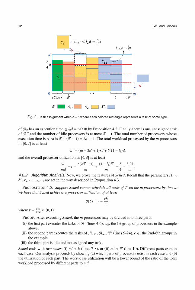
By the definition of A ′ in Equation (5) and Propositions 4.1 and 4.2, the 1st-2nd and 4th-6thgroups have an execution time in [𝑟𝑑, 𝑑]. The 3rd group of 𝛿 ′ processors executes a mix of the tasksof A3 and A2; the aggregate execution time of tasks is < 𝑟𝑑 but ≥ (1 − 𝑙2)𝑑 since the rejected task

12 Wu and Loiseau

Fig. 2. Task assignment when 𝛿 = 5 where each colored rectangle represents a task of some type.

of A2 has an execution time ≤ 𝑙2𝑑 = 3𝑑/10 by Proposition 4.2. Finally, there is one unassigned taskof A ′′ and the number of idle processors is at most 𝛿 ′ − 1. The total number of processors whoseexecution time is < 𝑟𝑑 is 𝛿 ′ + (𝛿 ′ − 1) = 2𝛿 ′ − 1. The total workload processed by the𝑚 processorsin [0, 𝑑] is at least

𝑤 ′ = (𝑚 − 2𝛿 ′ + 1)𝑟𝑑 + 𝛿 ′(1 − 𝑙2)𝑑,and the overall processor utilization in [0, 𝑑] is at least

𝑤 ′

𝑚𝑑= 𝑟 − 𝑟 (2𝛿 ′ − 1)

𝑚+ (1 − 𝑙2)𝛿

′

𝑚=34− 3.25

𝑚.

4.2.2 Algorithm Analysis. Now, we prove the features of 𝑆𝑐ℎ𝑒𝑑 . Recall that the parameters 𝐻 , a ,𝛿 ′, 𝑥a , · · · , 𝑥𝐻−1 are set in the way described in Proposition 4.3.

PROPOSITION 4.5. Suppose 𝑆𝑐ℎ𝑒𝑑 cannot schedule all tasks of T on the 𝑚 processors by time 𝑑 .We have that 𝑆𝑐ℎ𝑒𝑑 achieves a processor utilization of at least

\ (𝛿) = 𝑟 − 𝑟𝑘

𝑚.

where 𝑟 = 𝑢+1𝑢+2 ∈ (0, 1).

PROOF. After executing 𝑆𝑐ℎ𝑒𝑑 , the𝑚 processors may be divided into three parts:(i) the first part executes the tasks ofA ′ (lines 4-6), e.g, the 1st group of processors in the example

above,(ii) the second part executes the tasks of A𝑢+1, A𝑢 , A ′′ (lines 9-24), e.g., the 2nd-6th groups in

the example,(iii) the third part is idle and not assigned any task.

𝑆𝑐ℎ𝑒𝑑 ends with two cases: (i) 𝑚′ < 𝑘 (lines 7-8), or (ii) 𝑚′ < 𝛿 ′ (line 10). Different parts exist ineach case. Our analysis proceeds by showing (a) which parts of processors exist in each case and (b)the utilization of each part. The worst-case utilization will be a lower bound of the ratio of the totalworkload processed by different parts to𝑚𝑑 .

Efficient Approximation Algorithms for Scheduling Moldable Tasks 13

First, we analyze the utilization of the three parts. We have that (i) the first part of processors has autilization ≥ 𝑟 in [0, 𝑑] by the definition of A ′, and (ii) the utilization of the third part is zero. Thesecond part can be divided into several groups, each with 𝛿 ′ processors. Let A𝑢−1 = A ′′ for ease ofexposition. By lines 9-24, each group of the second part executes

(1) the tasks purely from a single set Aℎ where ℎ ∈ [𝑢 − 1, 𝑢 + 1], or(2) a mix of the tasks of multiple sets Aℎ , Aℎ−1, · · · , Aℎ′ where 𝑢 + 1 ≥ ℎ > ℎ′ ≥ 𝑢 − 1 and

ℎ′ ∈ {𝑢,𝑢 − 1}.In the former, we have that each group has an execution time ≥ 𝑟𝑑 by Propositions 4.1 and 4.2. Inthe latter, there exists a task 𝑇𝑗 of Aℎ′ that cannot be completed by time 𝑑:

(2.a) if ℎ′ = 𝑢, the group may have an execution time < 𝑟𝑑 but ≥ (1 − 𝑙𝑢)𝑑 since 𝑡 𝑗,𝛿′ < 𝑙𝑢𝑑

by Proposition 4.2 (see the third group in the example); by Proposition 4.3, the processedworkload is at least

𝑤 = 𝛿 ′(1 − 𝑙𝑢)𝑑 = (𝑢2 + 1)(1 − 𝑢

𝑢2 + 1𝑢 + 1𝑢 + 2

)𝑑 =

𝑢3 + 𝑢2 + 2𝑢 + 2 𝑑. (22)

(2.b) if ℎ′ = 𝑢 − 1, the group has an execution time ≥ 𝑟𝑑 since 𝑡 𝑗,𝛿′ < (1 − 𝑟 )𝑑 (see the fifth group inthe example).

To sum up, in the second part, there are at most 𝛿 ′ processors whose utilization is < 𝑟 in [0, 𝑑] andon which the amount of processed workload is ≥ 𝑤 .

Next, we analyze which parts of processors exist in each case when 𝑆𝑐ℎ𝑒𝑑 ends. In the first case,𝑆𝑐ℎ𝑒𝑑 ends at lines 7-8) and the first and third parts may exist. The third part has at most 𝑘 − 1 idleprocessors. Thus, the average utilization of the𝑚 processors is at least

𝑟1 =(𝑚 − 𝑘 + 1)𝑟𝑑

𝑚𝑑= 𝑟 − 𝑟 𝑘 − 1

𝑚.

In the second case, 𝑆𝑐ℎ𝑒𝑑 ends at line 10. All the three parts of processors may exist and the third parthas at most 𝛿 ′ − 1 processors. For the second part, there are at most 𝛿 ′ processors whose utilization is< 𝑟 . Thus, the average utilization of the𝑚 processors is at least

𝑟2 =𝑤 + (𝑚 − 𝛿 ′ − (𝛿 ′ − 1))𝑟𝑑

𝑚𝑑

(𝑎)= 𝑟 − 1

𝑚

( (2𝑢2 + 1

) 𝑢 + 1𝑢 + 2 −

𝑢3 + 𝑢2 + 2𝑢 + 2

)= 𝑟 − 1

𝑚

𝑢3 + 𝑢2 + 𝑢 − 1𝑢 + 2

(𝑏)= 𝑟 − 1

𝑚

(𝛿 ′𝑟 − 2

𝑢 + 2

)where the above (a) and (b) are due to Equation (22) and Proposition 4.3. Finally, when 𝑆𝑐ℎ𝑒𝑑 ends,a lower bound of the processor utilization is min{𝑟1, 𝑟2}, i.e.,

\ (𝛿) = 𝑟 −max{𝑟 (𝑘 − 1)

𝑚,1𝑚

(𝛿 ′𝑟 − 2

𝑢 + 2

)}(𝑐)≥ 𝑟 − 𝑟𝑘

𝑚(23)

where (c) is because 𝛿 ′ ≤ 𝛿 ≤ 𝑘 by Inequality (3a). □

PROPOSITION 4.6. The time complexity of 𝑆𝑐ℎ𝑒𝑑 is O(𝑛 log𝑚).

PROOF. The time complexity of task classification is O(𝑛 log𝑚) by Proposition 4.4 (line 1).Afterwards, the 𝑛 tasks are sequentially assigned to processors one by one (lines 5, 14) and 𝑆𝑐ℎ𝑒𝑑

stops until all tasks are assigned or there are not enough processors to assign the remaining tasks,which has a time complexity of O(𝑛). Hence, 𝑆𝑐ℎ𝑒𝑑 has a time complexity of O(𝑛 log𝑚). □

Given a set of tasks T , let S denote the subset of tasks accepted by Algorithm 1.

14 Wu and Loiseau

LEMMA 4.3. In Algorithm 1, we have for every task 𝑇𝑗 ∈ S that its workload is 𝐷 𝑗,𝛾 ( 𝑗,𝑑) , which isthe minimum workload needed to be processed to complete 𝑇𝑗 by time 𝑑 .

PROOF. 𝛾 ( 𝑗, 𝑑) is the minimum number of processors needed to complete 𝑇𝑗 by time 𝑑. ByProperty 3.1, 𝐷 𝑗,𝛾 ( 𝑗,𝑑) is the minimum workload needed to be processed to complete 𝑇𝑗 by time 𝑑 . InAlgorithm 1, the number of processors used to simultaneously execute a task is either 𝛾 ( 𝑗, 𝑑) for A ′or no more than 𝛿 for A𝑢+1, A𝑢 , and A ′′. For the latter, by Inequality (3a), we have for each task 𝑇𝑗that 𝛾 ( 𝑗, 𝑑) ≤ 𝐻 − 1 ≤ 𝛿 ′ ≤ 𝛿; by Property 3.1, the workload of 𝑇𝑗 keeps constant when the numberof assigned processors varies in [0, 𝛿] and we have in Algorithm 1 that the workload of 𝑇𝑗 equals𝐷 𝑗,𝛾 ( 𝑗,𝑑) . Thus, the lemma holds. □

With Proposition 4.5 and Lemma 4.3, we have completed the design of the scheduling algorithm𝑆𝑐ℎ𝑒𝑑 described in Section 3.

5 APPLICATION TO TWO OBJECTIVESIn this section, we apply 𝑆𝑐ℎ𝑒𝑑 to respectively minimize the makespan and maximize the through-

put with a common deadline 𝜏 .

5.1 Makespan MinimizationBuilt on 𝑆𝑐ℎ𝑒𝑑, we propose a binary search procedure to find a feasible schedule of all tasks

of T , called the OMS algorithm (Optimized MakeSpan). At its beginning, let 𝑈 and 𝐿 be suchthat 𝑆𝑐ℎ𝑒𝑑 can produce a feasible schedule of T by time 𝑈 but fails to do so by time 𝐿, e.g.,𝑈 = 𝑛(𝛿 + 2)max𝑇𝑗 ∈T{𝑡 𝑗,1} and 𝐿 = 0; we explain the reason why such 𝑈 is feasible in A. TheOMS algorithm will repeatedly execute the following operations, and stop when 𝑈 ≤ (1 + 𝜖)𝐿 where𝜖 ∈ (0, 1) is arbitrarily small:

(1) 𝑀 ← 𝑈 +𝐿2 ;

(2) if there exists a task 𝑇𝑗 ∈ T that cannot be completed by time 𝑀 on any of the𝑚 processors(i.e., 𝛾 ( 𝑗, 𝑀) = +∞) or 𝑆𝑐ℎ𝑒𝑑 fails to produce a feasible schedule of all tasks of T by time 𝑀 ,set 𝐿 ← 𝑀;

(3) otherwise, set 𝑈 ← 𝑀 , and 𝑆𝑐ℎ𝑒𝑑 produces a feasible schedule of T by time 𝑀 .When the algorithm stops, we have that (i) 𝑆𝑐ℎ𝑒𝑑 can produce a feasible schedule of T with amakespan ≤ 𝑈 but > 𝐿, and, (ii) 𝑈 ≤ (1 + 𝜖)𝐿.

In the rest of this subsection, we analyze the approximation ratio and complexity of the algorithm.As shown below, for a task 𝑇𝑗 , the larger the value of 𝑑 , the smaller the value of 𝛾 ( 𝑗, 𝑑).

LEMMA 5.1. If 𝑑 ′ < 𝑑 ′′, then we have 𝛾 ( 𝑗, 𝑑 ′) ≥ 𝛾 ( 𝑗, 𝑑 ′′).

PROOF. We prove this by contradiction. Suppose 𝛾 ( 𝑗, 𝑑 ′) < 𝛾 ( 𝑗, 𝑑 ′′); then we have by Property 3.1that 𝑡 𝑗,𝛾 ( 𝑗,𝑑′) ≥ 𝑡 𝑗,𝛾 ( 𝑗,𝑑′′) . Since 𝑡 𝑗,𝛾 ( 𝑗,𝑑′) ≤ 𝑑 ′ < 𝑑 ′′, the minimum number of processors needed tocomplete 𝑇𝑗 by time 𝑑 ′′ is no greater than 𝛾 ( 𝑗, 𝑑 ′), which contradicts the assumption that 𝛾 ( 𝑗, 𝑑 ′) <𝛾 ( 𝑗, 𝑑 ′′). □

Let 𝑑∗ denote the optimal makespan. In an optimal schedule, let 𝐷∗𝑗 denote the workload of a task𝑇𝑗 and 𝐷∗ denote the total workload of all tasks of T to be processed on the𝑚 processors in [0, 𝑑∗]where we have

𝑚𝑑∗ ≥ 𝐷∗ . (24)

When the OMS algorithm ends, if 𝛾 ( 𝑗, 𝐿) ∈ [1,𝑚] for every task 𝑇𝑗 ∈ T , only a part of tasks arescheduled by 𝑆𝑐ℎ𝑒𝑑 by time 𝐿 and we have by Proposition 4.5 that \ (𝛿) is a lower bound of the

Efficient Approximation Algorithms for Scheduling Moldable Tasks 15

processor utilization in [0, 𝐿]; we denote by 𝐷𝐿𝑗 the workload of a scheduled task 𝑇𝑗 and by 𝐷𝐿 the

total workload of all the scheduled tasks; here, we have

𝑚𝐿 ≥ 𝐷𝐿 ≥ \ (𝛿)𝑚𝐿. (25)

LEMMA 5.2. When the OMS algorithm ends, if 𝑑∗ < 𝐿, then we have that (i) 𝐷∗ ≥ 𝐷𝐿 and (ii)𝛾 ( 𝑗, 𝐿) ∈ [1,𝑚] for every task 𝑇𝑗 ∈ T .

PROOF. For every 𝑇𝑗 ∈ T , if 𝑑∗ < 𝐿, we have 𝛾 ( 𝑗, 𝐿) ∈ [1,𝑚] since 𝑇𝑗 can be finished by 𝑑∗.By Lemma 5.1, if 𝑑 ′ < 𝑑 ′′, we have 𝛾 ( 𝑗, 𝑑 ′) ≥ 𝛾 ( 𝑗, 𝑑 ′′). Since 𝑑∗ < 𝐿, we have in an optimalschedule that the number of processors assigned to a task 𝑇𝑗 is ≥ 𝛾 ( 𝑗, 𝑑∗), which is ≥ 𝛾 ( 𝑗, 𝐿). ByProperty 3.1, we have 𝐷∗𝑗 ≥ 𝐷 𝑗,𝛾 ( 𝑗,𝑑∗) ≥ 𝐷 𝑗,𝛾 ( 𝑗,𝐿) . By Lemma 4.3, we have 𝐷 𝑗,𝛾 ( 𝑗,𝐿) = 𝐷𝐿

𝑗 . Finally,we have 𝐷∗𝑗 ≥ 𝐷𝐿

𝑗 and 𝐷∗ ≥ 𝐷𝐿 . □

PROPOSITION 5.1. The OMS algorithm gives a 1\ (𝛿) (1 + 𝜖)-approximation to the makespan

minimization problem with a complexity of O(𝑛 log(𝑛/𝜖) log𝑚).

PROOF. We simply denote \ (𝛿) by \ . For the approximation ratio, it suffices to show 𝑈 /𝑑∗ ≤(1 + 𝜖)/\ where \ ∈ (0, 1]. When the OMS algorithm ends, we have

𝑈 ≤ (1 + 𝜖)𝐿. (26)

Obviously, 𝑑∗ ≤ 𝑈 . In the case that 𝑑∗ ∈ [𝐿,𝑈 ], we have

𝑈

𝑑∗≤ 1 + 𝜖 ≤ 1

\(1 + 𝜖).

In the other case that 𝑑∗ < 𝐿, we have by Inequalities (24), (25) and (26) and Lemma 5.2 that

𝑚𝑑∗ ≥ 𝐷∗ ≥ 𝐷𝐿 ≥ 𝑚\𝐿 ≥ 𝑚\𝑈

1 + 𝜖 .

Further, we have 𝑈 /𝑑∗ ≤ (1 + 𝜖)/\ .Finally, the initial values of 𝑈 and 𝐿 are 𝑛(𝛿 + 2)max𝑇𝑗 ∈T{𝑡 𝑗,1} and 0. The binary search stops

when 𝑈 ≤ 𝐿(1 + 𝜖) and the number of iterations is O(log(𝑛/𝜖)). At each iteration, 𝑆𝑐ℎ𝑒𝑑 is run andhas a time complexity O(𝑛 log𝑚) by Proposition 4.6. Finally, the OMS algorithm has a complexityO(𝑛 log(𝑛/𝜖) log𝑚). □

5.2 Throughput Maximization with a Common DeadlineLet 𝑣 ′𝑗 = 𝑣 𝑗/𝐷 𝑗,𝛾 ( 𝑗,𝜏) , and it is the maximum possible value obtained from processing a unit

of workload of 𝑇𝑗 , referred to as the (maximum) value density of 𝑇𝑗 . We assume without loss ofgenerality that

𝑣 ′1 ≥ 𝑣 ′2 ≥ · · · ≥ 𝑣 ′𝑛 .

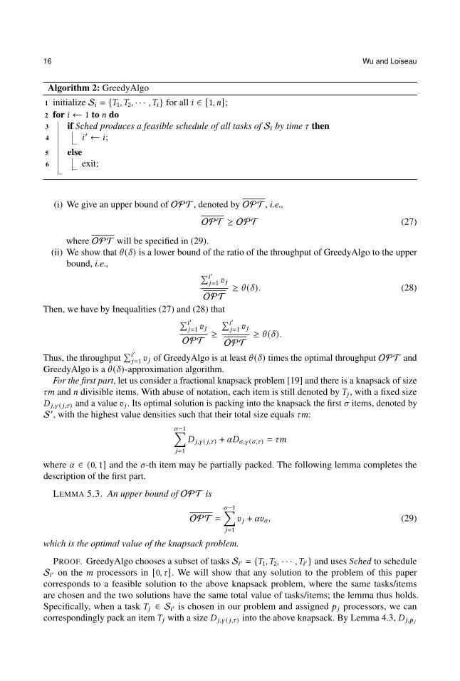
We propose a greedy algorithm called GreedyAlgo, presented in Algorithm 2: it considers tasks inthe non-increasing order of their value densities 𝑣 ′𝑗 and finally finds the maximum 𝑖 ′ such that 𝑆𝑐ℎ𝑒𝑑can output a feasible schedule by time 𝜏 for the first 𝑖 ′ tasks, denoted by S𝑖′ , but fails to do so for thefirst 𝑖 ′ + 1 tasks. The throughput of GreedyAlgo is

∑𝑖′𝑗=1 𝑣 𝑗 .

PROPOSITION 5.2. GreedyAlgo gives a \ (𝛿)-approximation to the throughput maximizationproblem with a common deadline and it has a complexity of O(𝑛2 log𝑚).

In the rest of this subsection, we give an overview of the proof of Proposition 5.2. By Proposi-tion 4.5, \ (𝛿) is a lower bound of the processor utilization when 𝑆𝑐ℎ𝑒𝑑 schedules S𝑖′ in [0, 𝜏]. LetOPT denote the optimal throughput of our problem. The proof of Proposition 5.2 has two parts:

16 Wu and Loiseau

Algorithm 2: GreedyAlgo

1 initialize S𝑖 = {𝑇1,𝑇2, · · · ,𝑇𝑖 } for all 𝑖 ∈ [1, 𝑛];2 for 𝑖 ← 1 to 𝑛 do3 if 𝑆𝑐ℎ𝑒𝑑 produces a feasible schedule of all tasks of S𝑖 by time 𝜏 then4 𝑖 ′← 𝑖;

5 else6 exit;

(i) We give an upper bound of OPT , denoted by OPT , i.e.,

OPT ≥ OPT (27)

where OPT will be specified in (29).(ii) We show that \ (𝛿) is a lower bound of the ratio of the throughput of GreedyAlgo to the upper

bound, i.e., ∑𝑖′𝑗=1 𝑣 𝑗

OPT≥ \ (𝛿). (28)

Then, we have by Inequalities (27) and (28) that∑𝑖′𝑗=1 𝑣 𝑗

OPT ≥∑𝑖′

𝑗=1 𝑣 𝑗

OPT≥ \ (𝛿).

Thus, the throughput∑𝑖′

𝑗=1 𝑣 𝑗 of GreedyAlgo is at least \ (𝛿) times the optimal throughput OPT andGreedyAlgo is a \ (𝛿)-approximation algorithm.

For the first part, let us consider a fractional knapsack problem [19] and there is a knapsack of size𝜏𝑚 and 𝑛 divisible items. With abuse of notation, each item is still denoted by 𝑇𝑗 , with a fixed size𝐷 𝑗,𝛾 ( 𝑗,𝜏) and a value 𝑣 𝑗 . Its optimal solution is packing into the knapsack the first 𝜎 items, denoted byS′, with the highest value densities such that their total size equals 𝜏𝑚:

𝜎−1∑︁𝑗=1

𝐷 𝑗,𝛾 ( 𝑗,𝜏) + 𝛼𝐷𝜎,𝛾 (𝜎,𝜏) = 𝜏𝑚

where 𝛼 ∈ (0, 1] and the 𝜎-th item may be partially packed. The following lemma completes thedescription of the first part.

LEMMA 5.3. An upper bound of OPT is

OPT =

𝜎−1∑︁𝑗=1

𝑣 𝑗 + 𝛼𝑣𝜎 , (29)

which is the optimal value of the knapsack problem.

PROOF. GreedyAlgo chooses a subset of tasks S𝑖′ = {𝑇1,𝑇2, · · · ,𝑇𝑖′} and uses 𝑆𝑐ℎ𝑒𝑑 to scheduleS𝑖′ on the 𝑚 processors in [0, 𝜏]. We will show that any solution to the problem of this papercorresponds to a feasible solution to the above knapsack problem, where the same tasks/itemsare chosen and the two solutions have the same total value of tasks/items; the lemma thus holds.Specifically, when a task 𝑇𝑗 ∈ S𝑖′ is chosen in our problem and assigned 𝑝 𝑗 processors, we cancorrespondingly pack an item 𝑇𝑗 with a size 𝐷 𝑗,𝛾 ( 𝑗,𝜏) into the above knapsack. By Lemma 4.3, 𝐷 𝑗,𝑝 𝑗

Efficient Approximation Algorithms for Scheduling Moldable Tasks 17

= 𝐷 𝑗,𝛾 ( 𝑗,𝜏) and∑

𝑇𝑗 ∈S𝑖′𝐷 𝑗,𝛾 ( 𝑗,𝜏) ≤ 𝜏𝑚; thus, the items 𝑇1, 𝑇2, · · · , 𝑇𝑖′ can successfully be packed into

the knapsack. □

For the second part, the detailed proof of (28) will be provided in B. Below, we provide theunderlying intuition while proving (28). The workload of each task𝑇𝑗 ∈ S𝑖′ accepted by GreedyAlgois also 𝐷 𝑗,𝛾 ( 𝑗,𝑑) by Lemma 4.3. S𝑖′ and S′ contain the first 𝑖 ′ and 𝜎 tasks with the highest valuedensities respectively. We have 𝑖 ′ ≤ 𝜎 since in GreedyAlgo the utilization of the 𝑚 processors in[0, 𝜏] is ≤ 1. Thus, the average value density of S𝑖′ is no smaller than the average value density ofS′, i.e., ∑𝑖′

𝑗=1 𝑣 𝑗∑𝑖′𝑗=1 𝐷 𝑗,𝛾 ( 𝑗,𝑑)

≥ OPT𝜏𝑚

.

Further, we can prove (28): ∑𝑖′𝑗=1 𝑣 𝑗

OPT≥

∑𝑖′𝑗=1 𝐷 𝑗,𝛾 ( 𝑗,𝑑)

𝜏𝑚≥ \ (𝛿).

Finally, Algorithm 2 considers S1, S2, · · · , S𝑛 one by one (line 2). Whenever 𝑆𝑐ℎ𝑒𝑑 attempts toschedule tasks on 𝑚 processor by time 𝜏 (line 3), it has a time complexity O(𝑛 log𝑚) by Proposi-tion 4.6. Hence, the complexity of GreedyAlgo is O(𝑛2 log𝑚).

6 CONCLUSIONSWe study the problem of scheduling 𝑛 independent moldable tasks on 𝑚 processors that arises

in large-scale parallel computations. When tasks are monotonic, the best known result is a ( 32 + 𝜖)-approximation algorithm for makespan minimization with a complexity linear in 𝑛 and polynomialin log𝑚 and 1

𝜖where 𝜖 is arbitrarily small. We propose a new perspective of the existing speedup

models: the speedup of a task 𝑇𝑗 is linear when the number 𝑝 of assigned processors is small (upto a threshold 𝛿 𝑗 ) while it presents monotonicity when 𝑝 ranges in [𝛿 𝑗 , 𝑘 𝑗 ]; the bound 𝑘 𝑗 indicatesan unacceptable overhead when parallelizing on too many processors. For a given integer 𝛿 ≥ 5,let 𝑢 =

⌈2√𝛿

⌉− 1. In this paper, we propose a 1

\ (𝛿) (1 + 𝜖)-approximation algorithm for makespan

minimization with a complexity O(𝑛 log(𝑛/𝜖) log𝑚) where \ (𝛿) = 𝑢+1𝑢+2

(1 − 𝑘

𝑚

)(𝑚 ≫ 𝑘). As a

by-product, we also propose a \ (𝛿)-approximation algorithm for throughput maximization with acommon deadline with a complexity O(𝑛2 log𝑚).

ACKNOWLEDGEMENTSThe work of Patrick Loiseau was supported by the French National Research Agency (ANR)

through the “Investissements d’avenir” program (ANR-15-IDEX- 02), and by the Alexander vonHumboldt Foundation.

REFERENCES[1] ARIDOR, Y., DOMANY, T., GOLDSHMIDT, O., KLITEYNIK, Y., MOREIRA, J., AND SHMUELI, E. (2005). Open jobmanagement architecture for the blue gene/l supercomputer. In Proceedings of the 11th Workshop on Job SchedulingStrategies for Parallel Processing. Springer, 91–107.

[2] BELKHALE, K. P. AND BANERJEE, P. (1990). An approximate algorithm for the partitionable independent task schedulingproblem. In Proceedings of the 1990 International Conference on Parallel Processing. Pennsylvania State University Press,72–75.

[3] BENOIT, A., LE FÈVRE, V., PEROTIN, L., RAGHAVAN, P., ROBERT, Y., AND SUN, H. (2020). Resilient scheduling ofmoldable jobs on failure-prone platforms. In Proceedings of the 22nd IEEE International Conference on Cluster Computing.IEEE, 81–91.

18 Wu and Loiseau

[4] BERG, B., VESILO, R., AND HARCHOL-BALTER, M. (2019). hesrpt: Optimal scheduling of parallel jobs with knownsizes. ACM SIGMETRICS Performance Evaluation Review 47, 2, 18–20.

[5] DECKER, T., LÜCKING, T., AND MONIEN, B. (2006). A 54 -approximation algorithm for scheduling identical malleable

tasks. Theoretical Computer Science 361, 2-3, 226–240.[6] DROZDOWSKI, M. (1996). Real-time scheduling of linear speedup parallel tasks. Information processing letters 57, 1,35–40.

[7] DROZDOWSKI, M. (2004). Scheduling Parallel Tasks – Algorithms and Complexity. CRC Press.[8] DUTTON, R. A., MAO, W., CHEN, J., AND WATSON III, W. (2008). Parallel job scheduling with overhead: A benchmarkstudy. In Proceedings of the IEEE International Conference on Networking, Architecture, and Storage. IEEE, 326–333.

[9] FISHKIN, A. V., GERBER, O., JANSEN, K., AND SOLIS-OBA, R. (2005). Packing weighted rectangles into a square. InProceedings of the 30th International Symposium on Mathematical Foundations of Computer Science. Springer, 352–363.

[10] HAVILL, J. T. AND MAO, W. (2008). Competitive online scheduling of perfectly malleable jobs with setup times.European Journal of Operational Research 187, 3, 1126–1142.

[11] HOCHBAUM, D. S. AND SHMOYS, D. B. (1987). Using dual approximation algorithms for scheduling problemstheoretical and practical results. Journal of the ACM 34, 1, 144–162.

[12] JAIN, N., MENACHE, I., NAOR, J. S., AND YANIV, J. (2015). Near-optimal scheduling mechanisms for deadline-sensitive jobs in large computing clusters. ACM Transactions on Parallel Computing 2, 1, 3.

[13] JANSEN, K. (2012). A ( 32 + 𝜖) approximation algorithm for scheduling moldable and non-moldable parallel tasks. InProceedings of the 24th annual ACM symposium on Parallelism in algorithms and architectures. ACM, 224–235.

[14] JANSEN, K. AND LAND, F. (2018). Scheduling monotone moldable jobs in linear time. In Proceedings of the IEEEInternational Parallel and Distributed Processing Symposium. IEEE, 172–181.

[15] JANSEN, K. AND PORKOLAB, L. (2002). Linear-time approximation schemes for scheduling malleable parallel tasks.Algorithmica 32, 3, 507–520.

[16] JANSEN, K. AND THÖLE, R. (2010). Approximation algorithms for scheduling parallel jobs. SIAM Journal onComputing 39, 8, 3571–3615.

[17] JANSEN, K. AND ZHANG, G. (2007). Maximizing the total profit of rectangles packed into a rectangle. Algorith-mica 47, 3, 323–342.

[18] JOHN, L. K. AND EECKHOUT, L. (2018). Performance evaluation and benchmarking. CRC Press.[19] KORTE, B. AND VYGEN, J. (2018). The Knapsack Problem. Springer, Berlin, Heidelberg, 471–487.[20] LUCIER, B., MENACHE, I., NAOR, J. S., AND YANIV, J. (2013). Efficient online scheduling for deadline-sensitive jobs.In Proceedings of the 25th ACM symposium on Parallelism in Algorithms and Architectures. ACM, 305–314.

[21] LUDWIG, W. AND TIWARI, P. (1994). Scheduling malleable and nonmalleable parallel tasks. In Proceedings of the fifthannual ACM-SIAM symposium on Discrete algorithms. ACM, 167–176.

[22] MOUNIÉ, G., RAPINE, C., AND TRYSTRAM, D. (1999). Efficient approximation algorithms for scheduling malleabletasks. In Proceedings of the 11th ACM symposium on Parallel algorithms and architectures. ACM, 23–32.

[23] MOUNIÉ, G., RAPINE, C., AND TRYSTRAM, D. (2007). A 32 -approximation algorithm for scheduling independent

monotonic malleable tasks. SIAM Journal on Computing 37, 2, 401–412.[24] STEINBERG, A. (1997). A strip-packing algorithm with absolute performance bound 2. SIAM Journal on Comput-ing 26, 2, 401–409.

[25] TUREK, J., WOLF, J. L., AND YU, P. S. (1992). Approximate algorithms scheduling parallelizable tasks. In Proceedingsof the fourth annual ACM symposium on Parallel algorithms and architectures. ACM, 323–332.

[26] WANG, Q. AND CHENG, K.-H. (1992). A heuristic of scheduling parallel tasks and its analysis. SIAM Journal onComputing 21, 2, 281–294.

[27] WIKIPEDIA. (2018). Supercomputer architechture. [accessed online, June 17, 2018],https://en.wikipedia.org/wiki/Supercomputer_architecture#21st-century_architectural_trends.

[28] WU, X. AND LOISEAU, P. (2015). Algorithms for scheduling deadline-sensitive malleable tasks. In Proceedings of the53rd Annual Allerton Conference on Communication, Control, and Computing. IEEE, 530–537.

[29] WU, X., LOISEAU, P., AND HYYTIÄ, E. (2019). Toward designing cost-optimal policies to utilize iaas clouds withonline learning. IEEE Transactions on Parallel and Distributed Systems 31, 3, 501–514.

A THE INITIAL VALUE OF 𝑈

The initial value of 𝑈 is set as

𝑈 = 𝑛(𝛿 + 2)max𝑇𝑗 ∈T{𝑡 𝑗,1},which is at least 𝛿 + 2 times the total execution time of all tasks when every task is assigned oneprocessor. 𝛾 ( 𝑗,𝑈 ) is the minimum number of processors needed to complete 𝑇𝑗 by time 𝑈 , and we

Efficient Approximation Algorithms for Scheduling Moldable Tasks 19

have 𝛾 ( 𝑗,𝑈 ) = 1 for all𝑇𝑗 ∈ T . We have by Inequality (3a) that 1 ≤ 𝐻 − 1 ≤ 𝛿 ′ ≤ 𝛿 . By Property 3.1,we have for every task 𝑇𝑗 ∈ T that

𝑡 𝑗,𝛿′ =𝑡 𝑗,1

𝛿 ′≤ 𝑈

𝑛(𝛿 + 2)𝛿 ′ ≤𝑈

𝛿 + 2 <𝑈

𝐻= (1 − 𝑟 )𝑈

where 𝑛 ≥ 1 and 𝑟 = 𝐻−1𝐻

. Every task of T has an execution time < (1 − 𝑟 )𝑑 when assigned 𝛿 ′

processors. Thus, all tasks of T are in the class A ′′, and the other classes A ′, A𝐻−1, · · · , Aa areempty. Now, we show that 𝑆𝑐ℎ𝑒𝑑 can produce a feasible schedule for all tasks of T by time 𝑈 .All tasks of T constitute A ′′ and will be sequentially executed on 𝛿 ′ processors (see lines 9-24 ofAlgorithm 1); the total execution time of T is ≤ 𝑛max𝑇𝑗 ∈T{𝑡 𝑗,1} ≤ 𝑈 .

B THE DETAILED PROOF OF THE SECOND PARTBelow, we formally prove Inequality (28). GreedyAlgo accepts the first 𝑖 ′ tasks with the highest

value densities 𝑣 ′𝑗 , and the achieved throughput is∑𝑖′

𝑗=1 𝑣 𝑗 . 𝑆𝑐ℎ𝑒𝑑 is used to schedule the 𝑖 ′ tasks, andeach accepted task 𝑇𝑗 has a workload 𝐷 𝑗,𝛾 ( 𝑗,𝜏) by Lemma 4.3. We denote by 𝜔 ∈ [0, 1] the actualutilization of the𝑚 processors in [0, 𝜏] achieved by GreedyAlgo, i.e.,

𝑖′∑︁𝑗=1

𝐷 𝑗,𝛾 ( 𝑗,𝜏) = 𝜔𝜏𝑚.

By Proposition 4.5, \ (𝛿) is a lower bound of the processor utilization and we have

𝜔 ≥ \ (𝛿) ∈ (0, 1] . (30)

Since 𝜔 ≤ 1, we have

𝑖 ′ ≤ 𝜎. (31)

LEMMA B.1. The throughput𝑖′∑𝑗=1

𝑣 𝑗 achieved by GreedyAlgo is at least \ (𝛿)OPT where OPT

is given in Equation (29).

PROOF. By Inequality (31), we will analyze two cases that 𝑖 ′ = 𝜎 and 𝑖 ′ < 𝜎 respectively. In thecase that 𝑖 ′ = 𝜎 , we have

𝑖′∑︁𝑗=1

𝑣 𝑗 ≤ OPT =

𝜎−1∑︁𝑗=1

𝑣 𝑗 + 𝛼𝑣𝜎

by Lemma 5.3. Thus, we have 𝛼 = 1 and the lemma holds.In the case that 𝑖 ′ < 𝜎 , let

𝑋1 =1𝜔

𝑖′∑︁𝑗=1

𝐷 𝑗,𝛾 ( 𝑗,𝜏) −𝑖′∑︁𝑗=1

𝐷 𝑗,𝛾 ( 𝑗,𝜏)

𝑋2 =

𝜎−1∑𝑗=𝑖′+1

𝐷 𝑗,𝛾 ( 𝑗,𝜏) + 𝛼𝐷𝜎,𝛾 ( 𝑗,𝜏) if 𝑖 ′ < 𝜎 − 1

𝛼𝐷𝜎,𝛾 ( 𝑗,𝜏) if 𝑖 ′ = 𝜎 − 1

𝑌 =

𝜎−1∑𝑗=𝑖′+1

𝑣 𝑗 + 𝛼𝑣𝜎 if 𝑖 ′ < 𝜎 − 1

𝛼𝑣𝜎 if 𝑖 ′ = 𝜎 − 1

20 Wu and Loiseau

Recall

𝜏𝑚 =1𝜔

𝑖′∑︁𝑗=1

𝐷 𝑗,𝛾 ( 𝑗,𝜏) =𝜎−1∑︁𝑗=1

𝐷 𝑗,𝛾 ( 𝑗,𝜏) + 𝛼𝐷𝜎,𝛾 (𝜎,𝜏) .

We thus have 𝑋1 = 𝑋2 since

𝜏𝑚 − 𝑋1 =

𝑖′∑︁𝑗=1

𝐷 𝑗,𝛾 ( 𝑗,𝜏) = 𝜏𝑚 − 𝑋2 .

The total value obtained by GreedyAlgo is𝑖′∑𝑗=1

𝑣 𝑗 and we have

𝑖′∑𝑗=1

𝑣 𝑗

𝜔𝜏𝑚

(𝑎)=

𝑖′∑𝑗=1

𝑣 ′𝑗( 1𝜔𝐷 𝑗,𝛾 ( 𝑗,𝜏) − 𝐷 𝑗,𝛾 ( 𝑗,𝜏) + 𝐷 𝑗,𝛾 ( 𝑗,𝜏)

)𝜏𝑚

(𝑏)≥

𝑖′∑𝑗=1

𝑣 𝑗 + 𝑣 ′𝑖′𝑋1

𝜏𝑚

(𝑐)=

𝑖′∑𝑗=1

𝑣 𝑗 + 𝑣 ′𝑖′𝑋2

𝜏𝑚

(𝑑)≥

𝑖′∑𝑗=1

𝑣 𝑗 + 𝑌

𝜏𝑚=OPT𝜏𝑚

.

(32)

Here, in Equation (a), 𝑣 𝑗 = 𝑣 ′𝑗𝐷 𝑗,𝛾 ( 𝑗,𝜏) ; Inequalities (b) and (d) are due to that 𝑣 ′1 ≥ · · · ≥ 𝑣 ′𝑖′ ≥ · · · ≥

𝑣 ′𝑛; Equation (c) is due to that 𝑋1 = 𝑋2. Due to Inequality (32), we have𝑖′∑𝑗=1

𝑣 𝑗 ≥ 𝜔OPT ; further, by

Inequality (30), the lemma holds. □